Shifting the Phase Transition Threshold for Random Graphs using Set Degree Constraints

Abstract

We show that by restricting the degrees of the vertices of a graph to an arbitrary set $\Delta$, the threshold point $\alpha(\Delta)$ of the phase transition for a random graph with $n$ vertices and $m=\alpha(\Delta)n$ edges can be either accelerated (e.g., $\alpha(\Delta)\approx 0.381$ for $\Delta=\{0,1,4,5\}$) or postponed (e.g., $\alpha(\{2^{0},2^{1},\cdots,2^{k},\cdots\})\approx 0.795$) compared to a classical Erdős–Rényi random graph with $\alpha(\mathbb{Z}_{\geq 0})=\tfrac{1}{2}$. In particular, we prove that the probability of graph being nonplanar and the probability of having a complex component, goes from $0$ to $1$ as $m$ passes $\alpha(\Delta)n$. We investigate these probabilities and also different graph statistics inside the critical window of transition (diameter, longest path and circumference of a complex component).

1 Introduction

1.1 Shifting the Phase Transition

Consider a random Erdős–Rényi graph $G(n,m)$ [ER60], that is a graph chosen uniformly at random among all simple graphs built with $n$ vertices labeled with distinct numbers from $\{1,2,\ldots,n\}$, and $m$ edges. The range $m=\tfrac{1}{2}n(1+\mu n^{-1/3})$ where $n\to\infty$, and $\mu$ depends on $n$, is of particular interest since there are three distinct regimes, according to how the crucial parameter $\mu$ grows as $n$ is large:

• as $\mu\to-\infty$, the size of the largest component is of order $\Theta(\log n)$, and the connected components are almost surely trees and unicyclic components;

• next, inside what is known as the critical window $|\mu|=O(1)$, the largest component size is of order $\Theta(n^{2/3})$ and complex structures (unempty set of connected components having strictly more edges than vertices) start to appear with significant probabilities;

• finally, as $\mu\to+\infty$ with $n$, there is typically a unique component of size $\Theta(n)$ called the giant component.

Since the article of Erdős and Rényi [ER60], various researchers have studied in depth the phase transition of the Erdős–Rényi random graph model culminating with the masterful work of Janson, Knuth, Łuczak, and Pittel [JKLP93] who used enumerative approach to analyze the fine structure of the components inside the critical window of $G(n,\,m)$.

The last decades have seen a growth of interest in delaying or advancing the phase transitions of random graphs. Mainly, two kinds of processes have been introduced and studied:

• the Achlioptas process where models of random graph are obtained by adding edge one by one but according to a given rule which allows to choose the next edge from a set of candidate edges [BF01, RW17],

• the given degree sequence models where a sequence $(d_{1},\,\cdots,\,d_{n})$ of degrees is given and a simple graph built on $n$ vertices is uniformly chosen from the set of all graphs whose degrees match with the sequence $d_{i}$ (see  [Rio12, MR95, HM12, JPRR16]).

In [BF01, RW12, RW17], the authors studied the Achlioptas process. Bohman and Frieze [BF01] were able to show that there is a random graph process such that after adding $m=0.535\,n>0.5\,n$ edges the size of the largest component is (still) polylogarithmic in $n$ which contrasts with the classical Erdős–Rényi random graphs. Initially, this process was conjectured to have a different local geometry of transition compared to classical Erdős–Rényi model, but Riordan and Warnke [RW12, RW17] were able to show that this is not the case. Next, in the model of random graphs with a fixed degree sequence $D=(d_{1},\,\cdots,\,d_{n})$, Joos, Perarnau, Rautenbach, and Reed [JPRR16] proved that a simple condition that a graph with degree sequence $D$ has a connected component of linear size, is that the sum of the degrees in $D$ which are not $2$ is at least $\lambda(n)$ for some function $\lambda(n)$ that goes to infinity with $n$.

In the current work, our approach is rather different. We study random graphs with degree constraints that are graphs drawn uniformly at random from the set of all graphs with given number of vertices and edges with all vertices having degrees from a given set $\Delta\subseteq\mathbb{Z}_{\geq 0}$, with the only restriction $1\in\Delta$, which we discuss below. De Panafieu and Ramos [dPR16] calculated asymptotic number of such graphs using methods from analytic combinatorics. Using their asymptotic results, we prove that random graphs with degrees from the set $\Delta$ have their phase transition shifted from the density of edges $\tfrac{m}{n}=\tfrac{1}{2}$ to $\tfrac{m}{n}=\alpha$ for an explicit and computable constant $\alpha=\alpha(\Delta)$ and the new critical window of transition becomes $m=\alpha n(1\pm\mu n^{-1/3})\,.$

In addition, we also prove that the structure of such graphs inside this crucial window behaves as in the Erdős–Rényi case. For instance, we prove that extremal parameters such as the diameter, the circumference or the longest path are of order $\Theta(n^{1/3})$ around $m=\alpha n$. The size of complex components of our graphs are of order $\Theta(n^{2/3})$ as $\mu$ is bounded. A very similar result but about the diameter of the largest component of $G(n,\,p=\frac{1}{n}+\frac{\mu}{n^{4/3}})$ has been obtained by Nachmias and Peres [NP08] (using very different methods).

In the seminal paper of Erdős and Rényi, amongst other non-trivial properties, they discussed the planarity of random graphs with various edge densities [ER60]. The probabilities of planarity of Erdős-Rényi random graphs inside their window of transition have been since then computed by Noy, Ravelomanana, and Rué [RRN13]. In the current work, we extend this study by showing that the planarity threshold shifts from $\frac{n}{2}$ for classical random graphs to $\alpha n$ for graphs with degrees from $\Delta$. More precisely, first we show that such objects are almost surely planar as $\mu$ goes to $-\infty$ and non-planar as $\mu$ tends to $+\infty$. Next, as function of $\mu$, we compute the limiting probability that random graphs of degrees in $\Delta$ are planar as $\mu=O(1)$.

Our work is motivated by the following research questions: (i) what can be the contributions of analytic combinatorics to study constrained random graphs? (ii) the birth of the giant component often corresponds to drastic changes in the complexities of several algorithmic optimization / decision problems on random graphs, so by tuning the thresholds one can shift the location of hard random instances.

1.2 Preliminaries

The excess of a connected graph is the number of its edges minus the number of its vertices. For example, connected graphs with excess $-1$ are trees, with excess $0$ — graphs with one cycle (also known as unicycles or unicyclic graphs), connected bicycles have excess $2$, and so on (see Figure 1). Connected graph always has excess at least $-1$. A connected component with excess at least $1$, is called a complex component. The complex part of a random graph is the union of its complex components.

           

Figure 1: Examples of connected labeled graphs with different excess. As a whole, can be considered as a graph with total excess $-1+0+1+2=2$

Next, we introduce the notion of a $2$-core (the core) and a $3$-core (the kernel) of a graph. The 2-core is obtained by repeatedly removing all vertices of degree $1$ (smoothing). The 3-core is obtained from 2-core by repeatedly replacing vertices of degree two with their adjacent edges by a single edge connecting the neighbors of deleted vertices (we call this a reduction procedure). A 3-core can be a multigraph, i.e. there can be loops and multiple edges. There is only a finite number of connected 3-cores with a given excess [JKLP93]. The inverse images of vertices of 3-core under the reduction procedure, are called corner vertices (cf. Figure 3). A 2-path is an inverse image of an edge in a $3$-core, i.e. a path connecting two corner vertices.

The circumference of a graph is the length of its longest cycle. A diameter of a graph is the maximal length of the shortest path taken over all distinct pairs of vertices. It is known that the problems of finding the longest path and the circumference are NP-hard.

Random graph with degree constraints is a graph sampled uniformly at random from the set of all possible graphs $\mathcal{G}_{n,m,\Delta}$ having $m$ edges and $n$ vertices all of degrees from the set $\Delta=\{\delta_{1},\delta_{2},\ldots\}\subseteq\{0,1,2,\ldots\}$, see Figure 2. The set $\Delta$ can be finite or infinite. In this work, we require that $1\in\Delta$. This technical condition allows the existence of trees and tree-like structures in the random objects under consideration. We don’t know what happens when $1\notin\Delta$.

Figure 2: Random labeled graph from $\mathcal{G}_{26,30,\Delta}$ with the set of degree constraints $\Delta=\{1,2,3,5,7\}$

The set $\mathcal{G}_{n,m,\Delta}$ is (asymptotically) nonempty if and only if the following condition is satisfied [dPR16]:

$(\mathcal{C})$

Denote $\mathrm{gcd}(d_{1}-d_{2}\colon d_{1},d_{2}\in\Delta)$ by periodicity $p$. Assume that the number $m$ of edges grows linearly with the number $n$ of vertices, with $2m/n$ staying in a fixed compact interval of $]\min(\Delta),\max(\Delta)[$, and $p$ divides ${2m-n\cdot\min(\Delta)}$.

To a given arbitrary set $\Delta\subseteq\{0,1,2,\ldots\}$, we associate the exponential generating function (egf) $\omega(z)$:

$$\mathrm{SET}_{\Delta}(z)=\omega(z)=\sum_{d\in\Delta}\dfrac{z^{d}}{d!}\enspace.$$ (1)

The domain of the argument $z$ of this function can be either considered a subset $[0,R)$ of the real axis or some subset of the complex plane, depending on the context. The function $\phi_{0}(z)=\frac{z\omega^{\prime}(z)}{\omega(z)}$, which is called the characteristic function of $\omega(z)$, is non-decreasing along real axis [FS09, Proposition IV.5], as well as the characteristic function $\phi_{1}(z)=\frac{z\omega^{\prime\prime}(z)}{\omega^{\prime}(z)}$ of the derivative $\omega^{\prime}(z)$.

The value of the threshold $\alpha$, which is used in all our theorems, is a unique solution of the system of equations

$$\begin{cases}\phi_{1}(\widehat{z})=1,\\ \phi_{0}(\widehat{z})=2\alpha.\end{cases}$$ (2)

A unique solution $\widehat{z}$ of $\phi_{1}(z)=1,z>0$ always exists provided that $1\in\Delta$. This solution is computable.

Structure of the Article.

In section 2 we state our main results and give proofs which rely on technical statements from Appendix A. In section 3, we give the results of simulations using the recursive method from [dPR16]. Section A contains the tools from analytic combinatorics. Then follows Appendix B with the method of moments and marking tools.

2 Phase Transition for Random Graphs

2.1 Structure of Connected Components

Recall that given a set $\Delta$, its egf is defined as $\omega(z)=\sum_{d\in\Delta}z^{d}/d!$, and characteristic function of $\omega(z)$ and its derivative $\omega^{\prime}(z)$ are given by $\phi_{0}(z)=z\omega^{\prime}(z)/\omega(z)$, $\phi_{1}(z)=z\omega^{\prime\prime}(z)/\omega^{\prime}(z)$.

Theorem .

Given a set $\Delta$ with $1\in\Delta$, let $\alpha$ be a unique positive solution of (2). Assume that $m=\alpha n(1+\mu n^{-1/3})$. Suppose that Condition Preliminaries is satisfied and $G_{n,m,\Delta}$ is a random graph from $\mathcal{G}_{n,m,\Delta}$.

Then, as $n\to\infty$, we have

1. if $\mu\to-\infty$, $|\mu|=O(n^{1/12})$, then

   $$\mathbb{P}(G_{n,m,\Delta}\text{\emph{ has only trees and unicycles}})=1-\Theta(|\mu|^{-3})\enspace;$$ (3)

2. if $|\mu|=O(1)$, i.e. $\mu$ is fixed, then

   $$\mathbb{P}(G_{n,m,\Delta}\text{\emph{ has only trees and unicycles}})\to\mbox{constant}\in(0,1)\enspace,$$ (4)

   $$\mathbb{P}(G_{n,m,\Delta}\text{\emph{ has a complex part with total excess }}q)\to\mbox{constant}\in(0,1),$$ (5)

   and the constants are computable functions of $\mu$;

3. if $\mu\to+\infty$, $|\mu|=O(n^{1/12})$, then

   $$\mathbb{P}(G_{n,m,\Delta}\text{\emph{ has only trees and unicycles}})=\Theta(e^{-\mu^{3}/6}\mu^{-3/4})\enspace,$$ (6)

   $$\mathbb{P}(G_{n,m,\Delta}\text{\emph{ has a complex part with excess }}q)=\Theta(e^{-\mu^{3}/6}\mu^{3q/2-3/4})\enspace.$$ (7)

Proof (Sketched).

Consider a graph composed of trees, unicycles and a collection of complex connected components. Fix the total excess of complex components $q$. Then, there are exactly $(n-m+q)$ trees, because each tree has an excess $-1$.

Generating functions for each of these components are given by subsection A.1 and subsection A.1: we enumerate all possible kernels and then enumerate graphs that reduce to them under pruning and smoothing. Let $U(z)$ be the generating function for unrooted trees, $V(z)$ be the generating function for unicycles, $E_{j}(z)$ be the generating functions for connected graphs with excess $j$. We calculate the probability for each collection $(q_{1},\ldots,q_{k})$, while the total excess is $\sum_{j=1}^{k}jq_{j}=q$. Accordingly, the probability that the process generates a graph with the described property can be expressed as the ratio

$$\dfrac{n!\cdot|\mathcal{G}_{n,m,\Delta}|^{-1}}{(n-m+q)!}[z^{n}]U(z)^{n-m+q}e^{V(z)}\dfrac{E_{1}^{q_{1}}(z)}{q_{1}!}\ldots\dfrac{E^{q_{k}}_{k}(z)}{q_{k}!}\enspace.$$ (8)

Then we use an approximation of $E_{j}(z)$ from subsection A.1, subsection A.1 and apply subsection A.2 with $y=\tfrac{1}{2}+3q$ in order to extract the coefficients. Note that our approach is derived from the methods from [JKLP93], and so some of our proofs are sketched. ∎

2.2 Shifting the Planarity Threshold

Theorem .

Under the same conditions as in subsection 2.1 with a number of edges $m=\alpha n(1+\mu n^{-1/3})$, let $p(\mu)$ be the probability that $G_{n,m,\Delta}$ is planar.

Then, as $n\to\infty$, we have uniformly for $|\mu|=O(n^{1/12})$:

1. $p(\mu)=1-\Theta(|\mu|^{-3})$, as $\mu\to-\infty$;

2. $p(\mu)\to\mbox{constant}\in(0,1)$, as $|\mu|=O(1)$, and $p(\mu)$ is computable;

3. $p(\mu)\to 0$, as $\mu\to+\infty$.

Proof.

The graph is planar if and only if all the 3-cores (multigraphs) of connected complex components are planar. As $|\mu|=O(n^{1/12})$, subsection A.1 implies that for asymptotic purposes it is enough to consider only cubic regular kernels among all possible planar 3-cores. Let $G_{1}(z)$ be an egf of connected planar cubic kernels. The function $G_{1}(z)$ is determined by the system of equations given in [RRN13], and is computable. An egf for sets of such components is given by $G(z)=e^{G_{1}(z)}$. We give several first terms of $G(z)$ according to [RRN13]:

$$G(z)=\sum_{q\geq 0}g_{q}\dfrac{z^{2q}}{(2q)!^{2}}=1+\dfrac{5}{24}z^{2}+\dfrac{385}{1152}z^{4}+\dfrac{83933}{82944}z^{6}+\dfrac{35002561}{7962624}z^{8}+\ldots$$ (9)

Thus, the number of planar cubic kernels with total excess $q$ is given by

$$(2q)![z^{2q}]e^{G_{1}(z)}=(2q)![z^{2q}]G(z)=\dfrac{g_{q}}{(2q)!}\enspace.$$

In order to calculate $p(\mu)$, we sum over all possible $q\geq 0$ and multiply the probabilities that the 3-core is a planar cubic graph with excess $q$ by the conditional probability that a random graph has planar cubic kernel of excess $q$.

The probability that $G_{n,m,\Delta}$ is planar on condition that the excess of the complex component is $q$, is equal to

$$\dfrac{n!|\mathcal{G}_{n,m,\Delta}|^{-1}}{(n-m+q)!}[z^{n}]U(z)^{n-m+q}e^{V(z)}\dfrac{g_{q}}{(2q)!}\dfrac{(T_{3}(z))^{2r}}{(1-T_{2}(z))^{3r}}\enspace.$$ (10)

We can apply subsection A.2 and sum over all $q\geq 0$ in order to obtain the result:

$$p(\mu)\sim\sqrt{2\pi}\sum_{q\geq 0}g_{q}t_{3}^{2q}A_{\Delta}(3q+\tfrac{1}{2},\mu)\enspace,$$ (11)

where $A_{\Delta}(3q+\tfrac{1}{2},\mu)$ and the constant $t_{3}$ are from subsection A.2. The probabilities on the borders of the transition window, i.e. $|\mu|\to\infty$ can be obtained from the properties of the function $A_{\Delta}(y,\mu)$. ∎

2.3 Statistics of the Complex Component Inside the Critical Window

Theorem .

Under the same conditions as in subsection 2.1, suppose that ${|\mu|=O(1)}$, $m=\alpha n(1+\mu n^{-1/3})$. Then, the longest path, diameter and circumference of the complex part are of order $\Theta(n^{1/3})$ in probability, i.e. for each mentioned random parameter there exist computable (see subsection B.1) constants $A,B>0$ depending on $\Delta$ such that the corresponding random variable $X_{n}$ satisfies $\forall\lambda>0$

$$\mathbb{P}\left(X_{n}\notin n^{1/3}(A\pm B\lambda)\right)=O(\lambda^{-2})\enspace.$$ (12)

Figure 3: Diameter, longest path and circumference of a complex component. The large vertices like are the corner vertices

Proof.

Recall that a 2-path is a path connecting two corner vertices inside a complex component, see Figure 3. In subsection B.1 we prove that the length of a randomly uniformly chosen 2-path is $\Theta(n^{1/3})$ in probability. This lemma also gives the explicit expressions for $A$ and $B$.

From subsection B.2 we obtain that the maximum height of sprouting tree over the complex part is also $\Theta(n^{1/3})$ in probability. Since the total excess of the complex component is bounded in probability as $\mu$ stays bounded, and the sizes of the kernels are finite, we can combine these two results to obtain the statement of the theorem, because all the three parameters come from adding/stitching several $2$-paths and tree heights.

∎

3 Simulations

We considered random graphs with $n=1000$ vertices, and various degree constraints. The random generation procedure of such graphs has been explained by de Panafieu and Ramos in [dPR16] and for our experiments, we implemented the recursive method. We note that this kind of sampling is not exact in the sense that the probability of obtaining a simple graph is uniform only in asymptotics.

The generator first draws a sequence of degrees and then performs a random pairing on half-edges, as in configuration model [Bol80]. We reject the pairing until the multigraph is simple, i.e. until there are no loops and multiple edges. As $|\mu|=O(1)$, expected number of rejections is asymptotically $\exp\left(-\frac{1}{2}\phi_{1}(\widehat{z})-\frac{1}{4}\phi_{1}^{2}(\widehat{z})\right)$ , which is $\exp(-3/4)$ in the critical window, and in the subcritical phase it is less.

Each sequence $(d_{1},\ldots,d_{n})$ is drawn with weight $\prod_{v=1}^{n}1/(d_{v})!$. First, we use dynamic programming to precompute the sums of the weights $(S_{i,j})\colon{i\in[0,n]}$, ${j\in[0,2m]}$ using initial conditions and the recursive expression:

$$S_{i,j}=\sum_{\overset{d_{1}+\ldots+d_{i}=j}{d_{1},\ldots,d_{i}\in\Delta}}\prod_{v=1}^{i}\dfrac{1}{d_{v}!}\enspace,\quad S_{i,j}=\begin{cases}1,&(i,j)=(0,0)\enspace,\\ 0,&i=0\text{ or }j<0\enspace,\\ \sum\limits_{d\in\Delta}\dfrac{S_{i-1,j-d}}{d!},&\text{otherwise}\enspace.\end{cases}$$ (13)

Then the sequence of degrees is generated according to the distribution

$$\mathbb{P}(d_{n}=d)=\dfrac{S_{n-1,2m-d}}{d!S_{n,2m}}\enspace.$$ (14)

We made plots for distributions of different parameters for $\Delta=\{1,3,5,7\}$, see Figure 4.

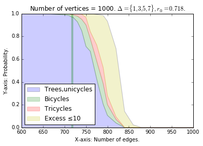
(a) Largest excess

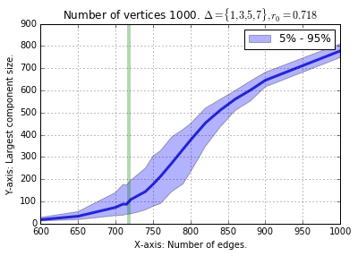
(b) Largest component size

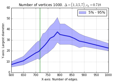
(c) Graph diameter

Figure 4: Results of experiments

Conclusion.

We studied how to shift the phase transition of random graphs when the degrees of the nodes are constrained by means of analytic combinatorics [dPR16, FS09].

We have shown that the planarity threshold of those constrained graphs can be shifted generalizing the results in [RRN13]. We have also shown that when our random constrained graphs are inside their critical window of transition, the size of complex components are typically of order $n^{2/3}$ and all distances inside the complex components are of order $n^{1/3}$, thus our results about these parameters complement those of Nachmias and Peres [NP08].

A few open questions are left open: for given threshold value $\alpha$ can we find a set $\{1\}\subset\Delta\subset\mathbb{Z}_{\geq 0}$ delivering the desired $\alpha$? What happens if $1\notin\Delta$, for example what is the structure of random Eulerian graphs? What happens when the generating function $\omega$ itself depends on the number of vertices? Given a sequence of degrees $d_{1},\ldots,d_{n}$ that allows the construction of a forest of an unbounded size, a first approach to study possible relationship between the models can be the computation of the generating function $\omega(z)=\sum_{i\geq 0}\mathrm{weight}(i)\dfrac{z^{i}}{i!}$ for a suitable weight function corresponding to $d_{1},\ldots,d_{n}$.

Acknowledgements.

We would like to thank Fedor Petrov for his help with subsection A.2, Élie de Panafieu, Lutz Warnke, and several anonymous referees for their valuable remarks.

Appendix A Saddle-point Analysis

A.1 Symbolic Tools

For each $r\geq 0$, let us define $r$-sprouted trees: rooted trees whose vertex degrees belong to the set $\Delta$, except the root (see Figure 5), whose degree belongs to the set
$\Delta-\ell=\{\delta\geq 0\colon\delta+\ell\in\Delta\}$. Their egf $T_{\ell}(z)$ can be defined recursively

$$T_{\ell}(z)=z\omega^{(\ell)}(T_{1}(z)),\ T_{1}(z)=z\omega^{\prime}(T_{1}(z))\enspace,\quad\ell\geq 0\enspace.$$ (15)

Lemma .

Let $U(z)$ be the egf for unrooted trees and $V(z)$ the EGF of unicycles whose vertices have degrees $\in\Delta$. Then

$$U(z)=T_{0}(z)-\dfrac{T_{1}(z)^{2}}{2}\enspace,\quad V(z)=\dfrac{1}{2}\left[\log\dfrac{1}{1-T_{2}(z)}-T_{2}(z)-\dfrac{T_{2}^{2}(z)}{2}\right]\enspace,$$ (16)

where $T_{0}(z)$, $T_{1}(z)$, and $T_{2}(z)$ are by (15).

$T_{0}\begin{cases}\phantom{r}\\ \phantom{r}\\ \phantom{r}\\ \phantom{r}\\ \phantom{r}\end{cases}$ $T_{1}\begin{cases}\phantom{r}\\ \phantom{r}\end{cases}$

Figure 5: Recursive construction of $T_{0}(z)$: the degree of the root of each subtree should belong to the set $\Delta-1$

Remark .

The above statement for $U(z)$ can be proven using the dissymetry theorem for trees, adapted for the case with degree constraints (see [BLL98, Section 4.1], [FPK89]). In short, we can consider rooted trees $T_{0}$ and mark the vertex with label $1$. Then we consider two cases, when this vertex is the root one, or not. The first case corresponds to $U(z)$ and in the second situation we can consider two subcases, whether the label $1$ belongs to the subtree induced by the first child or not (see Figure 6). Summarizing the argument, we obtain

$$T_{0}(z)=U(z)+\dfrac{1}{2}T_{1}(z)^{2}\enspace.$$

Figure 6: Variant of dissymetry theorem for unrooted trees with degree constraints

The expression for $V(z)$ is an application of the symbolic method of EGFs in the case of undirected cycles (cyc_≥3) of $2$-sprouted trees, see Figure 7.

Figure 7: Unicycles with degree constraints

Any multigraph $M$ on $n$ labeled vertices can be defined by a symmetric $n\times n$ matrix of nonnegative integers $m_{xy}$, where $m_{xy}=m_{yx}$ is the number of edges $x-y$ in $M$. The compensation factor $\kappa(M)$ is defined by

$$\kappa(M)=1\left/\prod_{x=1}^{n}\left(2^{m_{xx}}\prod_{y=x}^{n}m_{xy}!\right)\right.\enspace.$$ (17)

A multigraph process is a sequence of $2m$ independent random vertices

$$(v_{1},v_{2},\ldots,v_{2m})\enspace,\quad v_{k}\in\{1,2,\ldots,n\}\enspace,$$

and output multigraph with the set of vertices $\{1,2,\ldots,n\}$ and the set of edges $\{\{v_{2i-1},v_{2i}\}\colon 1\leq i\leq m\}$. The number of sequences that lead to the same multigraph $M$ is exactly $2^{m}m!\kappa(M)$.

Lemma .

Let $\overline{\overline{M}}$ be some 3-core multigraph with a vertex set $V$, $|V|=n$, having $\mu$ edges, and compensation factor $\kappa(\overline{\overline{M}})$. Let $\mu_{xy}$ be the number of edges between vertices $x$ and $y$ for $1\leq x\leq y\leq n$. The generating function for all graphs $G$ that lead to $\overline{\overline{M}}$ under reduction is

$$\dfrac{\kappa(\overline{\overline{M}})\displaystyle\prod\limits_{v\in V}T_{\deg(v)}(z)}{n!}\cdot\dfrac{P(\overline{\overline{M}},T_{2}(z))}{(1-T_{2}(z))^{\mu}};$$ (18)

$$P(\overline{\overline{M}},z)=\prod_{x=1}^{n}\Big{(}z^{2\mu_{xx}}\!\!\!\!\prod_{y=x+1}^{n}\!\!\!\!z^{\mu_{xy}-1}(\mu_{xy}-(\mu_{xy}-1)z)\Big{)}.$$ (19)

Corollary .

Assume that $\phi_{1}(\widehat{z})=1$. Near the singularity $z\sim\widehat{z}$, i.e. $T_{2}(z)\approx 1$, some of the summands from subsection A.1 are negligible. Dominant summands correspond to graphs $\overline{\overline{M}}$ with maximal number of edges, i.e. graphs with $3r$ edges and $2r$ vertices. The vertices of degree greater than $3$ can be splitted into more vertices with additional edges. Due to [JKLP93, Section 7, Eq. (7.2)], the sum of the compensation factors is expressed as

$$e_{r0}=\dfrac{(6r)!}{2^{5r}3^{2r}(3r)!(2r)!}\enspace.$$ (20)

and the sum of major summands is asymptotically

$$e_{r0}\dfrac{T_{3}(z)^{2r}}{(1-T_{2}(z))^{3r}}\enspace.$$ (21)

The proofs of the two previous statements are postponed until the end of subsection A.1.

Remark .

Let’s give an example of application of subsection A.1, first in less technical multigraph form, then for simple graphs.

Each multi-edge in the 3-core $\overline{\overline{M}}$ corresponds to a sequence of trees in the initial graph $M$. Therefore, the generating function for multigraphs $M$ which reduce to one of the three depicted (see Figure 8) 3-core multigraphs consists of 3 summands:

$$W_{\Delta}(z)=\dfrac{1}{4}\dfrac{T_{4}(z)}{(1-T_{2}(z))^{2}}+\dfrac{1}{4}\dfrac{T_{3}(z)^{2}}{(1-T_{2}(z))^{3}}+\dfrac{1}{6}\dfrac{T_{3}(z)^{2}}{(1-T_{2}(z))^{3}}\enspace.$$ (22)

       

Figure 8: All possible 3-core multigraphs of excess $1$ and their compensation factors. The first one has negligible contribution because it is non-cubic

We write $T_{2}(z)$ because if we attach a tree on any path, the degree of the root decreases by $2$. For the same reason there appear $T_{3}(z)$ and $T_{4}(z)$. If we evaluate $W_{\Delta}(z)$ near the pole $z=\widehat{z}$, or equivalently at $T_{2}(z)=1$, the first summand goes to $\infty$ slower than the second and the third. This yields asymptotic approximation

$$W_{\Delta}(z)=\dfrac{5}{24}\dfrac{T_{3}(z)^{2}}{(1-T_{2}(z))^{3}}+O\left(\dfrac{1}{(1-T_{2}(z))^{2}}\right)\enspace.$$ (23)

The big-O notation with the generating functions means:

$$F(z)=O(B(z))\text{ if }[z^{n}]F(z)\leq c[z^{n}]B(z)$$ (24)

for sufficiently large $n$, so from Eq. (23) we know that

$$[z^{n}]W_{\Delta}(z)\sim[z^{n}]\dfrac{5}{24}\dfrac{T_{3}(z)^{2}}{(1-T_{2}(z))^{3}}\enspace.$$ (25)

With simple graphs (not multigraphs) the situation is similar. For the first core we want the path to be non-empty (because simple graphs don’t contain loops), so the generating function is $\dfrac{1}{4}\dfrac{T_{4}(z)T_{2}(z)^{4}}{(1-T_{2}(z))^{2}}$. For the second graph we also require that both paths obtained from loops, contain at least one node inside: $\dfrac{1}{4}\dfrac{T_{3}(z)^{2}T_{2}(z)^{4}}{(1-T_{2}(z))^{3}}$. Then, for the third core, we need at least two of the paths contain at least one node. Collecting all the summands we obtain

$$\widetilde{W}_{\Delta}(z)=\dfrac{1}{4}\dfrac{T_{4}(z)T_{2}(z)^{4}}{(1-T_{2}(z))^{2}}+\dfrac{1}{4}\dfrac{T_{3}(z)^{2}T_{2}(z)^{4}}{(1-T_{2}(z))^{3}}+\dfrac{1}{6}\dfrac{T_{3}(z)^{2}[3T_{2}(z)^{2}-2T_{2}^{3}(z)]}{(1-T_{2}(z))^{3}}\enspace.$$ (26)

At $z$ near $\widehat{z}$, $T_{2}(z)=1$, so the asymptotics of this term is again

$$\widetilde{W}_{\Delta}(z)=\dfrac{5}{24}\dfrac{T_{3}(\widehat{z})^{2}}{(1-T_{2}(z))^{3}}+O\left(\dfrac{1}{(1-T_{2}(z))^{2}}\right)\enspace.$$ (27)

In the similar manner as was done in [JKLP93, Lemma 2, Eq. (9.21)], we can prove that the dominant summand in the case of simple graphs and multigraphs is the same and equals the total compensation factor of cubic kernels $e_{r0}$ times the generating function $\dfrac{T_{3}(z)^{\text{\#nodes}}}{(1-T_{2}(z))^{\text{\#edges}}}$. We omit the factor $T_{2}(z)^{\text{\#edges}}$ because it is equal to $1$ (as $z=\widehat{z}$).

Proof of subsection A.1.

The proof is similar to [JKLP93, Lemma 2]. We need to count the junctions of different degrees. All the paths contain vertices of degree at least 2, so we plug $T_{2}(z)$ into $P(\overline{\overline{M}},z)$. ∎

Proof of subsection A.1.

(From [Bol85, Chapter 2]) In a cubic multigraph each vertex has 3 half-edges that need to be paired, there are $6r$ half-edges in total. The number of such pairings is $(6r)!/\left((3r)!2^{3r}\right)$. In each vertex the three half-edges can be permuted in $3!=6$ ways, so we divide by $6^{2r}$ to obtain finally that

$$\text{the number of cubic multigraphs}=\dfrac{(6r)!}{(3r)!2^{3r}6^{2r}}\enspace.$$ (28)

The multiple $(2r)!$ appears because the graph has $2r$ vertices and we deal with exponential generating functions. ∎

A.2 Analytic Tools

Remark .

The crucial tool that we use in our work is the analytic lemma, subsection A.2, or equivalently, subsection A.2. Since the statements are quite cubersome, we propose an alternative way to understand the statements, by dividing the quantities involved into this theorem.

Suppose that $|\mu|=O(1)$, and $n\to\infty$. We treat $A_{\Delta}(y,\mu)$ as a nearly constant number, while for the asymptotics the important factor is $n^{y/3-1/2}$ with ${y=3r+1/2}$. The left-hand side of Eq. (32) expresses the probability of graph having complex component of excess $r$, provided that we specify the function $\Psi$ correctly according to our combinatorial specification.

When we increase the excess $r$ by $1$, the exponential index of $n^{y/3-1/2}$ increases by $1$, and the expression is multiplied by $n$. This is exactly the combinatorial interpretation that we are looking for: the generating functions of graphs which reduce to kernels that are non-cubic, have a negligible contribution into the total probability.

In order to count the number of graphs with complex component of excess $r$, we note that the total number of trees should compensate the total excess to $m-n$, so the number of trees is $n-m+r$. When we substitute this into subsection A.2, additional multiple $n$ caused by extra excess, cancels with $(n-m+r)!$ in the denominator. This explains why for any fixed collection of excesses of complex components $q_{1},q_{2},\ldots,q_{k}$ the probability of having a graph with such an excess, is asymptotically a constant. A rigorous calculation of this probability involves substituting the asymptotics of $|\mathcal{G}_{n,m,\Delta}|$ obtained in [dPR16].

Lemma .

Let $m=rn=\alpha n(1+\mu\nu)$, where $\nu=n^{-1/3}$, $|\mu|=O(n^{1/12})$, $n\to\infty$, and $\widehat{z}$ be a unique real positive solution of ${\phi_{1}(\widehat{z})=1}$. Let

$$C_{2}=\dfrac{t_{3}\alpha\widehat{z}}{2(1-\alpha)},\quad C_{3}=\dfrac{2t_{3}\alpha\widehat{z}}{3},\quad t_{3}=\dfrac{\widehat{z}\omega^{\prime\prime\prime}(\widehat{z})}{\omega^{\prime}(\widehat{z})}.$$

Then for any function $\tau(z)$ analytic in $|z|\leq\widehat{z}$ the contour integral encircling complex zero, admits asymptotic representation

$$\dfrac{1}{2\pi i}\oint(1-\phi_{1}(z))^{1-y}e^{nh(z;r)}\tau(z)\dfrac{dz}{z}\sim\left.\nu^{2-y}(zt_{3})^{1-y}\tau(z)e^{nh(z;\alpha)}\times B_{\Delta}(y,\mu)\right|_{z=\widehat{z}}\enspace,$$ (29)

$$B_{\Delta}(y,\mu) = \frac{1}{3}C_{3}^{(y-2)/3}\displaystyle\sum\limits_{k\geq 0}\dfrac{\left(C_{2}C_{3}^{-2/3}\mu\right)^{k}}{k!\Gamma\left(\frac{y+1-2k}{3}\right)}$$

$$h(z;r) = \log\omega^{\prime}-r\log z+(1-r)\log\left(2\dfrac{\omega}{\omega^{\prime}}-z\right)$$

The proof of the current lemma will be given below.

Remark .

In order to compute the probability in subsection A.2, we express the coefficient of a generating function as a contour integral. The methods for computing integrals of such kind are well-developed, for example, in [PW13]. In case of single root $z_{0}$ of the derivative $h_{z}(z;r)$ we approximate the integral with Gaussian density:

$$\dfrac{1}{2\pi i}\oint g(z)e^{nh(z;r)}\dfrac{dt}{t}\sim\left(\dfrac{1}{2\pi n}\right)^{1/2}\dfrac{g(z_{0})}{z_{0}\sqrt{h^{\prime\prime}(z_{0})}}e^{nh(z_{0})}$$ (30)

and in case of double root we approximate the integral of exponential of $(z-z_{0})^{3}$.

Therefore,

$$\dfrac{1}{2\pi i}\oint g(z)e^{nh(z;r)}\dfrac{dt}{t}\sim\dfrac{1}{2\pi i}\oint g(z)\exp\left(nh(z_{0};r)+nh^{(3)}_{z}(z_{0};r)\dfrac{(z-z_{0})^{3}}{6}\right)\dfrac{dt}{t}\enspace.$$ (31)

Though these techniques are quite standard in a certain community, this machinery cannot be directly applied to the case of degree constraints because we need to prove that on the circle $z=z_{0}e^{i\theta}$, $\theta\in[0,2\pi]$ the maximum is attained at point $\theta=0$, otherwise this method is not applicable.

Corollary .

If $m=\alpha n(1+\mu n^{-1/3})$ and $y\in\mathbb{R}$, $y\geq\tfrac{1}{2}$, then for any $\Psi(t)$ analytic at $t=1$ we have

$$\dfrac{n!}{(n-m)!|\mathcal{G}_{n,m,\Delta}|}[z^{n}]\dfrac{U(z)^{n-m}\Psi(T_{2}(z))}{(1-T_{2}(z))^{y}}=\sqrt{2\pi}\Psi(1)A_{\Delta}(y,\mu)n^{y/3-1/6}+O(R)\enspace,$$ (32)

$B_{\Delta}(y,\mu)$ is from subsection A.2 and the error term $R$ is given by ${R=(1+|\mu|^{4})n^{y/3-1/2}}$. This function $A_{\Delta}(y,\mu)$ can be expressed in terms of $A(y,\mu)=A_{\mathbb{Z}_{\geq 0}}(y,\mu)$ introduced in [JKLP93]:

1. $A_{\Delta}(y,\mu)=(t_{3}\widehat{z})^{1-y}(3C_{3})^{\tfrac{y-2}{3}}A\left(y,\dfrac{2C_{2}}{\sqrt[3]{(3C_{3})^{2}}}\mu\right)=e^{-\mu^{3}/6}(\widehat{z}t_{3})^{1-y}B_{\Delta}(y,\mu);$

2. As $\mu\to-\infty$, we have $A(y,\mu)=\dfrac{1}{\sqrt{2\pi}|\mu|^{y-1/2}}\left(1-\dfrac{3y^{2}+3y-1}{6|\mu|^{3}}+O(\mu^{-6})\right);$

3. As $\mu\to+\infty$, we have $A(y,\mu)=\dfrac{e^{-\mu^{3}/6}}{2^{y/2}\mu^{1-y/2}}\left(\dfrac{1}{\Gamma(y/2)}+\dfrac{4\mu^{-3/2}}{3\sqrt{2}\Gamma(y/2-3/2)}+O(\mu^{-2})\right)\enspace.$

Proof of subsection A.2 and subsection A.2.

Let us prove the corollary first. We start with “Stirling” approximation part. In case of classical random graphs it would be enough to apply the Stirling approximation, but in the case of degree constraints we apply the asymptotic result of [dPR16]:

$$\dfrac{n!}{(n-m)!|\mathcal{F}_{n,m,\Delta}|}=\sqrt{2\pi n}\dfrac{z_{0}^{2m}\sqrt{2\alpha}}{p\cdot\omega(z_{0})^{n}}\times\\ \exp(n\log n+(n-m)\log(n-m)-m\log 2m)\times\\ \exp(\tfrac{1}{2}\phi_{1}(z_{0})+\tfrac{1}{4}\phi_{1}^{2}(z_{0}))(1+O(n^{-1}))\enspace.$$

It happens that the exponential part of Stirling and some terms that will appear in Cauchy approximation, cancel out:

$$\exp\left(n\log n+(n-m)\log(n-m)\!-m\log 2m\right)=e^{-\mu^{3}/6}\times\frac{\omega(z_{0})^{n}}{z_{0}^{2m}}2^{m-n}e^{nh(\widehat{z};\alpha)}\enspace.$$ (33)

Let us move to the Cauchy part for obtaining formal series coefficients. After “Lagrangian” variable change $T_{1}(z)\mapsto z$ we obtain:

$$[z^{n}]\dfrac{U(z)^{n-m}\Psi(T_{2}(z))}{(1-T_{2}(z))^{y}}=\dfrac{1}{2\pi i}\oint\dfrac{\Psi(T_{2})U(z)^{n-m}dz}{(1-T_{2}(z))^{y}z^{n+1}}=\dfrac{2^{m-n}}{2\pi i}\oint\Psi(\phi_{1}(z))(1-\phi_{1}(z))^{1-y}e^{nh(z;r)}\dfrac{dz}{z}\enspace.$$

The statement readily follows from subsection A.2.

Let us prove the lemma then. We start with specifying an integration contour, namely the circle $z=\widehat{z}e^{-s\nu}$ where $s=\beta+it$, $\beta>0$, $t\in[-\pi n^{1/3},\pi n^{1/3}]$. We need $\beta\to 0$ with $n\to\infty$. Technically, for correct error estimate, $\beta$ can be chosen from

$$\mu=\beta^{-1}-\beta\enspace,$$ (34)

as suggested by [JKLP93]. We need to switch to contour $t\in(-\infty,+\infty)$ with the price of exponentially small error $O(e^{-\max(2,|\mu|)n^{1/6}/3})$, we omit the details of this approximation since they are already considered in the mentioned article.

Next, there will be two variable changes. The first change of variables is $z=\widehat{z}e^{-s\nu}$. We use an approximation for $nh(z;r)$ near the double saddle $\widehat{z}$ and critical ratio $\alpha$. From subsection A.2 it follows that maximum value of $|e^{nh(z,r)}|$ for $t\in[-\pi n^{1/3},\pi n^{1/3}]$ is attained for $t=0$ (and also at the points $\tfrac{2\pi ik}{d}\nu$ where $d$ is a period of $\Delta$, but we can assume without loss of generality that $d=1$, because otherwise, extra terms cancel out when we count the probability, since the denominator is given by expression from [dPR16]). Thus, we can choose a small $t_{0}>0$, such that $nh^{\prime\prime}(\widehat{z})(\nu t_{0})^{2}\to\infty$, $nh^{\prime\prime\prime}(\widehat{z})(\nu t_{0})^{3}\to 0$, and the absolute value of integral for $|t|>t_{0}$ is negligible.

Since there is a relation $r=\alpha(1+\mu\nu)$, we can use a Taylor expansion for $h(z,r)$ for $z$ around $\widehat{z}$, which is uniform with respect to $(\alpha-r)$:

$$h(z;r)=\sum_{k=0}^{3}\dfrac{h^{(k)}_{z}(\widehat{z};r)(z-\widehat{z})^{k}}{k!}+O\left((s\nu)^{4}\right)\enspace.$$ (35)

The first derivative turns to zero, the second and the third can be written as

$$h^{\prime\prime}(\widehat{z},r)=\dfrac{(\phi_{0}(\widehat{z})-2r)\phi_{1}^{\prime}(\widehat{z})}{\widehat{z}(\phi_{0}(\widehat{z})-2)}=\dfrac{t_{3}(\alpha-r)}{\widehat{z}(\alpha-1)}\enspace,$$ (36)

$$h^{\prime\prime\prime}(\widehat{z},r)=\dfrac{\phi_{0}^{\prime}(\widehat{z})\phi_{1}^{\prime}(\widehat{z})}{\widehat{z}(\alpha-1)}+O(\mu\nu)\sim-\dfrac{4t_{3}\alpha}{\widehat{z}^{2}}\enspace,$$ (37)

hence the final approximation takes the form

$$\!nh(z;r)\!=\!nh(\widehat{z};\alpha)+C_{2}\mu s^{2}+C_{3}s^{3}+O\left((\mu^{2}s^{2}\!+\!s^{4})\nu\right),$$ (38)

where $C_{2}=h^{\prime\prime}(\widehat{z};\alpha)\widehat{z}^{2}/2$ and $C_{3}=-h^{\prime\prime\prime}(\widehat{z};\alpha)\widehat{z}^{3}/6$ are given in the formulation. We also have

$$(1-\phi_{1}(z))^{1-y}=s^{1-y}\nu^{1-y}(1+O(s\nu))\enspace,$$

so when $s=O(n^{1/12})$, the integrand can be approximated

$$(1-\phi_{1}(z))^{1-y}e^{nh(z,r)}=\nu^{1-y}s^{1-y}e^{nh(\widehat{z};\alpha)}\times e^{C_{2}\mu s^{2}+C_{3}s^{3}}(1+O(s\nu)+O(\mu^{2}s^{2}\nu)+O(s^{4}\nu))\enspace,$$

therefore

$$\dfrac{1}{2\pi i}\oint(1-\phi_{1}(z))^{1-y}e^{nh(z;r)}\tau(z)\dfrac{dz}{z}=\dfrac{1}{2\pi i}(\nu\widehat{z}\phi_{1}^{\prime}(\widehat{z}))^{1-y}\tau(\widehat{z})e^{nh(\widehat{z})}\times\oint s^{1-y}e^{C_{2}\mu s^{2}+C_{3}s^{3}}\cdot(-\nu)ds\enspace.$$

Then we perform a second change of variable ${s=u^{1/3}C_{3}^{-1/3}}$. We need to be careful with the contour of integration: note that the integral doesn’t change if we take instead of $t\in[-\infty,+\infty]$ any path $\Pi(\beta),\beta>0$ given by

$$s(t)=\begin{cases}-e^{-\pi i/3}t,&-\infty<t\leq 2\beta;\\ \beta+it\sin\pi/3,&-2\beta\leq t\leq 2\beta;\\ e^{\pi i/3}t,&2\beta\leq t<+\infty.\end{cases}$$ (39)

After variable transform we obtain Hankel contour $\Gamma$ extending from $-\infty$, circling the origin counterclockwise, and returning to $-\infty$, and $ds=\tfrac{1}{3}(C_{3}u^{2})^{-1/3}du$.

$$\dfrac{1}{2\pi i}\int_{\Pi(\beta)}(\cdots)=\nu^{2-y}(\widehat{z}\phi_{1}^{\prime}(\widehat{z}))^{1-y}\tau(\widehat{z})e^{nh(\widehat{z};\alpha)}C_{3}^{-y/3}\times\dfrac{1}{2\pi i}\int_{\Gamma}u^{y/3}e^{u}e^{C_{2}\mu u^{2/3}C_{3}^{-2/3}}du\cdot\tfrac{1}{3}C_{3}^{-1/3}\enspace.$$

Expanding the exponent

$$e^{C_{2}C_{3}^{-2/3}\mu u^{2/3}}=\sum_{k\geq 0}(C_{2}C_{3}^{-2/3}\mu u^{2/3})^{k}/k!$$ (40)

and applying the formula for inverse Gamma function on approximate Hankel contour we obtain the final statement. ∎

Lemma .

Assume that $m=rn$. The coefficient at $z^{n}$ of an egf for graphs from $\mathcal{F}_{n,m,\Delta}$ given by an equation

$$[z^{n}]\dfrac{U(z)^{n-m+q}}{(n-m+q)!}e^{V(z)}E_{\mathbf{q}}(z)\enspace,$$ (41)

can be expressed as

$$\dfrac{2^{m-n}}{2\pi i(n-m+q)!}\oint e^{nh(z;r)}g(z)\tau(z)\dfrac{dz}{z}\enspace,$$ (42)

where the contour contains $0$, the functions $h(z;r)$, $g(z)$ are given by

$$h(z;r)=r\log\omega^{\prime}(z)-r\log z+(1-r)\log(2\omega-z\omega^{\prime}),$$ (43)

$$g(z)=(1-\phi_{1}(z))^{1-y}\ ,\enspace y=3q+\tfrac{1}{2}$$ (44)

and $\tau(z)$ doesn’t have singularities in $|z|\leq\widehat{z}$.

Proof.

We can do a variable change $T_{1}(z)=t\mapsto z$.
From the equation ${T_{1}(z)=z\omega^{\prime}(T_{1}(z))}$ we obtain:

$$z = t\omega^{\prime}(t)^{-1}\mapsto z\omega^{\prime}(z)^{-1},$$ (45)

$$dz = (\omega^{\prime})^{-1}(1-\phi_{1})dt,$$ (46)

$$T_{\ell} = z\omega^{(\ell)}(t)=t\omega^{(\ell)}(t)\omega^{\prime}(t)^{-1},$$ (47)

$$T_{2}(z) \mapsto \phi_{1}(z)\enspace,$$ (48)

$$U(z)^{n-m} \mapsto 2^{m-n}z^{n-m}(2\omega(\omega^{\prime})^{-1}-z)^{n-m}$$ (49)

Then, we separate out the singular part:

$$U(z)^{q}e^{V(z)}E_{\mathbf{q}}(z)\dfrac{dz}{z}=\underbrace{(1-T_{2}(z))(\omega^{\prime})^{-1}}_{dz/dt}\underbrace{\omega^{\prime}(t)t^{-1}}_{z^{-1}}$$ (50)

$$\times\underbrace{U(z)^{q}\sqrt{1-T_{2}(z)}e^{V(z)}}_{\tau_{1}(z)}\underbrace{(1-T_{2}(z))^{3q}E_{\mathbf{q}}(z)}_{\tau_{2}(z)}$$ (51)

$$\times\dfrac{1}{(1-T_{2}(z))^{3q}}\cdot\dfrac{1}{\sqrt{1-T_{2}(z)}}dt\mapsto\tau(z)g(z)\enspace,$$ (52)

and the exponential one:

$$U(z)^{n-m}z^{-n}\mapsto 2^{m-n}\left(2\dfrac{\omega}{\omega^{\prime}}-z\right)^{n-m}z^{n-m}\left(\dfrac{\omega^{\prime}}{z}\right)^{n}=2^{m-n}e^{nh(z;r)}\enspace.\qquad\quad$$ (53)

∎

In this section we mainly establish some asymptotic properties of $h(z;r)$ around $z=\widehat{z}$ and $r=r_{0}=\alpha$. Its behaviour is important for saddle-point techniques. At arbitrary point $r=\alpha(1+\mu n^{-1/3})$ its derivative factors as

$$h^{\prime}_{z}(z;r)=\dfrac{(\phi_{0}(z)-2r)(\phi_{1}(z)-1)}{z(\phi_{0}(z)-2)}\enspace,$$ (54)

and the dominant complex root of $h^{\prime}_{z}(z;r)$ (closest to zero) is a positive real number which is either the solution of $\phi_{0}(z)=2r$ or the solution of ${\phi_{1}(z)=1}$. Each of the equations has unique real positive solution which we denote by $\mathrm{Root}_{1}(r)$ and $\mathrm{Root}_{2}=\widehat{z}$, see Figure 9.

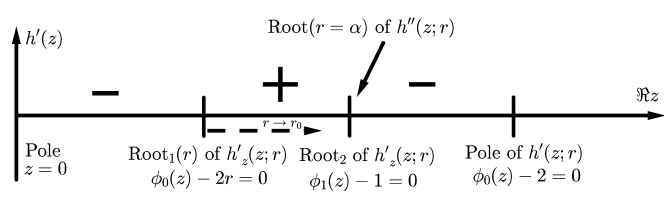
Figure 9: Configuration of roots of $h_{z}(z;r)$

Lemma .

Let $z_{0}>0$, $z_{0}\leq\min(\mathrm{Root}_{1}(r),\mathrm{Root}_{2})$, the periodicity of $\Delta$ is $p$. Then the function

$$\Phi(\theta;r)=\mathrm{Re}\;h(z_{0}e^{i\theta};r)$$ (55)

attains its global maximums for $\theta\in[0,2\pi)$ at $p$ points $\theta_{k}=\frac{2\pi k}{p}$, $k=0,1,\ldots,p-1$.

Proof.

Denote $z_{0}e^{i\theta}$ by $z$. Without loss of generality we will treat the case of aperiodic $\omega(z)$, since any $p$-periodic function $\pi(z)$ can be reduced to an aperiodic one $\varphi(z)$ by a variable change $\pi(z)=z^{\ell}\varphi(z^{p})$. $\Phi(\theta;r)$ can be rewritten as

$$\Phi(\theta;r)=r\log|\omega^{\prime}(z)|+(1-r)\log|2\omega-z\omega^{\prime}|+C\enspace.$$ (56)

We apply a version of Gibbs inequality for Kullback-Leibler divergence, also known as cross-entropy inequality: if $p_{1},p_{2},q_{1},q_{2}$ are positive real numbers and $q_{1}+q_{2}\leq p_{1}+p_{2}$ then

$$p_{1}\log\dfrac{p_{1}}{q_{1}}+p_{2}\log\dfrac{p_{2}}{q_{2}}\geq 0\enspace.$$ (57)

It is now sufficient to prove that

$$r\cdot\left|\dfrac{\omega^{\prime}(z)}{\omega^{\prime}(z_{0})}\right|+(1-r)\cdot\left|\dfrac{2\omega(z)-z\omega^{\prime}(z)}{2\omega(z_{0})-z_{0}\omega^{\prime}(z_{0})}\right|\leq 1\enspace.$$ (58)

Note that $\phi_{0}(z_{0})\leq 2r$. We first prove the inequality for $\widetilde{r}=\tfrac{1}{2}\phi_{0}(z_{0})$. Since the function $\omega^{\prime}(z)$ has non-negative coefficients, we always have $|\omega^{\prime}(z)/\omega^{\prime}(z_{0})|\leq 1$, therefore if $r$ increases, the inequality still remains true, thus for all $r\geq\widetilde{r}$ it is also true.

Substituting $\phi_{0}(z_{0})=z_{0}\omega^{\prime}(z_{0})\omega(z_{0})^{-1}=2r$ we arrive to more simple inequality

$$|z\omega^{\prime}(z)|+|2\omega(z)-z\omega^{\prime}(z)|\leq 2\omega(z_{0})\enspace,\quad z_{0}\leq\alpha\enspace.$$ (59)

This inequality was proven by Fedor Petrov at mathoverflow [Pet16] using a beautiful geometric statement.

Let $\gamma>\beta>0$ and $1/\beta-1/\gamma\geq 2$, then for any vector $z$ with $|z|=1$

$$|1+\gamma z|+|1-\beta z|\leq 2+\gamma-\beta\enspace.$$ (60)

Let us denote $z=e^{it}$. Differentiating the expression by $\theta$ and finding the zeros, we obtain

$$\dfrac{-2\gamma\sin\theta}{|1+\gamma z|}+\dfrac{2\beta\sin\theta}{|1+\beta z|}=0\enspace,$$ (61)

which is equivalent to

$$|z+1/\gamma|=|z-1/\beta|\enspace,$$ (62)

but the middle point of the segment $[-1/\gamma,1/\beta]$ has value greater than or equal to $1$ provided that $1/\beta-1/\gamma\geq 2$, so the perpendicular bisector to this segment doesn’t contain non-real points. The geometric statement in now proven.

Let $\omega(z)=\sum_{k\geq 0}c_{k}z^{k}$. Since $\phi_{1}(\widehat{z})=1$ and $0<|z|\leq\widehat{z}$, the inequality $\phi_{1}(z)\leq 1$ can be expanded as

$$c_{1}\geq\sum_{k\geq 2}(k^{2}-1)c_{k+1}|z|^{k}\enspace,$$ (63)

and we need to prove (59), which is equivalent to

$$\left|\sum_{k\geq 1}kc_{k}z^{k}\right|+|2c_{0}+c_{1}z-c_{3}z^{3}-2c_{4}z^{4}-\ldots|\leq 2c_{0}+2c_{1}|z|+2c_{2}|z|^{2}+\ldots$$ (64)

This is reduced by applying triangle inequality for removing terms with $c_{0}$ and $c_{2}$ and dividing by $|z|$:

$$|c_{1}+3c_{3}z^{3}+\ldots|+|c_{1}-c_{3}z^{2}-2c_{4}z^{3}-\ldots|\leq 2c_{1}+2c_{3}|z|^{2}+\ldots$$ (65)

Repeatedly using triangle inequalities, the above can be reduced to a family of inequalities

$$|(k^{2}-1)|z|^{k}+(k+1)z^{k}|+|(k^{2}-1)|z|^{k}-(k-1)z^{k}|\leq(2(k^{2}-1)+2)|z|^{k}\enspace,$$ (66)

which is a partial case of the geometric statement with $\gamma=\tfrac{1}{k-1}$, $\beta=\tfrac{1}{k+1}$. ∎

Appendix B Method of Moments

In order to study the parameters of random structures, we apply the marking procedure introduced in [FS09]. We say that the variable $u$ marks the parameter of random structure in bivariate egf $F(z,u)$ if $n![z^{n}u^{k}]F(z,u)$ is equal to number of structures of size $n$ and parameter equal to $k$. In this section we consider such parameters of a random graph as the length of $2$-path, which corresponds to some edge of the $3$-core, and the height of random “sprouting” tree. If we treat the parameter as a random variable $X_{n}$ then the factorial moments can be calculated through an expression

$$\mathbb{E}X_{n}(X_{n}-1)\ldots(X_{n}-k+1)=\dfrac{\left.\dfrac{d^{k}}{du^{k}}F(z,u)\right|_{u=1}}{F(z,1)}\enspace.$$ (67)

Recall that the number of graphs having $n$ vertices, $m$ edges, and fixed excess vector $\mathbf{q}=(q_{1},q_{2},\ldots)$, can be expressed as $n$-th coefficient of the generating function

$$\dfrac{U(z)^{n-m+q}}{(n-m+q)!}e^{V(z)}E_{\mathbf{q}}(z)\enspace,$$ (68)

where $E_{\mathbf{q}}(z)=\prod_{j=1}^{k}\frac{(E_{j}(z))^{q_{j}}}{q_{j}!}$, ${q=\sum_{j=1}^{k}jq_{j}}$. This egf can be modified to count the moments of random variable $X_{n}$.

B.1 Length of a Random 2-path

Let us fix the excess vector $\mathbf{q}=(q_{1},q_{2},\ldots,q_{k})$. There are in total $q=q_{1}+2q_{2}+\ldots+kq_{k}$ connected complex components and each component has one of the finite possible number of 3-cores (see [JKLP93]). We can choose any $2$-path, which is a sequence of trees, and replace it with of sequence of marked trees, see Figure 10. Let random variable $P_{n}$ be the length of this $2$-path. Since an egf for sequence of trees is $\tfrac{1}{1-T_{2}(z)}$, the corresponding moment-generating function $\mathbb{E}[u^{P_{n}}]$ becomes

$$\mathbb{E}[u^{P_{n}}]=\dfrac{n![z^{n}]\dfrac{U(z)^{n-m+q}}{(n-m+q)!}e^{V(z)}E_{\mathbf{q}}(z)\dfrac{1-T_{2}(z)}{1-uT_{2}(z)}}{n![z^{n}]\dfrac{U(z)^{n-m+q}}{(n-m+q)!}e^{V(z)}E_{\mathbf{q}}(z)}\enspace.$$ (69)

Figure 10: Marked 2-path inside complex component of some graph

Lemma .

Suppose that conditions of subsection 2.1 are satisfied. Suppose that there are $q_{j}$ connected components of excess $j$ for each $j$ from $1$ to $k$. Denote by excess vector a vector $\mathbf{q}=(q_{1},q_{2},\ldots,q_{k})$. Inside the critical window $m=\alpha n(1+\mu n^{-1/3})$, $|\mu|=O(1)$, the length $P_{n}$ of a random (uniformly chosen) $2$-path is $\Theta(n^{1/3})$ in probability, i.e.

$$\mathbb{P}\left(P_{n}\notin n^{1/3}t_{3}(B_{1}\pm\lambda B_{2})\right)\leq\dfrac{1}{(\lambda+o(1))^{2}}\enspace,$$ (70)

$$t_{3}=\widehat{z}\dfrac{\omega^{\prime\prime\prime}(\widehat{z})}{\omega^{\prime}(\widehat{z})}\enspace,\quad B_{1}=\dfrac{B_{\Delta}(3q+\tfrac{3}{2},\mu)}{B_{\Delta}(3q+\tfrac{1}{2},\mu)}\enspace,$$

$$B_{2}^{2}=\dfrac{B_{\Delta}(3q+\tfrac{5}{2},\mu)B_{\Delta}(3q+\tfrac{1}{2},\mu)-B_{\Delta}^{2}(3q+\tfrac{3}{2},\mu)}{B_{\Delta}^{2}(3q+\tfrac{1}{2},\mu)},$$

with function $B_{\Delta}(y,\mu)$ from subsection A.2, $q=q_{1}+2q_{2}+\ldots+kq_{k}$.

Proof.

The statement of the lemma is just an application of Chebyshev’s inequality to the first and the second moment. Essentially, we need to prove that

$$\mathbb{E}P_{n}\sim n^{1/3}t_{3}\dfrac{B_{\Delta}(3q+\tfrac{3}{2},\mu)}{B_{\Delta}(3q+\tfrac{1}{2},\mu)}\ ,\enspace\mathbb{E}P_{n}(P_{n}-1)\sim n^{2/3}\,\,2\,t_{3}^{2}\dfrac{B_{\Delta}(3q+\tfrac{5}{2},\mu)}{B_{\Delta}(3q+\tfrac{1}{2},\mu)}\enspace,$$ (71)

which is just a consequence of subsection A.2 and Eq. (67). ∎

B.2 Height of a Random Sprouting Tree

Let $\varkappa(z)=\omega^{\prime}(z)$. Consider recursive definition for the generating function of simple trees whose height doesn’t exceed $h$:

$$T^{[h+1]}(z)=z\varkappa(T^{[h]}(z))\ ,\enspace T^{[0]}(z)=0\enspace.$$ (72)

The framework of multivariate generating functions allows to mark height with a separate variable $u$ so that the function

$$F(z,u)=\sum_{n=0}^{\infty}\dfrac{z^{n}}{n!}\sum_{h=0}^{n}A^{[h]}_{n}u^{h}$$ (73)

is the bgf for trees, where $A^{[h]}_{n}$ stands for the number of simple labelled rooted trees with $n$ vertices, whose height equals $h$.

Flajolet and Odlyzko [FO82] consider the following expressions:

$$H(z)=\left.\dfrac{d}{du}F(z,u)\right|_{u=1},\enspace D_{s}(z)=\left.\dfrac{d^{s}}{du^{s}}F(z,u)\right|_{u=1}.$$ (74)

Generally speaking, $H(z)=D_{1}(z)$ is a particular case of $D_{s}(z)$, but their analytic behaviour is different for $s=1$ and $s\geq 2$.

Lemma ([FO82, pp. 42–50]).

The functions $H(z)$ and $D_{s}(z)$, $s\geq 2$ satisfy

$$H(z)\sim\alpha\log\varepsilon(z)\ ,\enspace D_{s}(z)\sim(\widehat{z})^{-1}s\Gamma(s)\zeta(s)\varepsilon^{-s+1}(z)\enspace,$$ (75)

$\alpha=2\dfrac{\varkappa^{\prime}(\widehat{z})}{\varkappa^{\prime\prime}(\widehat{z})}$, $\varepsilon(z)=\widehat{z}\left(1-\dfrac{z}{\rho}\right)^{1/2}\left(\dfrac{2\varkappa^{\prime\prime}(\widehat{z})}{\varkappa(\widehat{z})}\right)^{1/2}$, $\rho=\widehat{z}\varkappa^{-1}(\widehat{z})=(\varkappa^{\prime}(\widehat{z}))^{-1}$.

Here, $\Gamma(s)$ is a gamma-function, and $\zeta(s)$ is Riemann zeta-funciton.

We don’t represent their proof here, but would like to remark that it has great methodological impact. For our purposes we need the asymptotic equivalence $\sim$ only in the circle of analiticity $|z|<\rho$.

Recall that

$$T_{1}(z)=z\omega^{\prime}(T_{1}(z))\enspace,\quad T_{\ell}(z)=z\omega^{(\ell)}(T_{1}(z))\enspace,\quad\ell\geq 0$$ (76)

From local expansion at $z=\rho$ of $z=z(T_{1})$ it is easy to show that

$$z\sim\rho-(T_{1}(z)-\widehat{z})^{2}\left(\dfrac{\varkappa^{\prime\prime}(\widehat{z})\widehat{z}}{2\varkappa^{2}(\widehat{z})}\right)$$ (77)

and consequently, since $T_{k}(z)=z\varkappa^{(k)}(T_{1}(z))$,

$$T_{1}(z) = \widehat{z}-\sqrt{\dfrac{2\varkappa}{\varkappa^{\prime\prime}}}\sqrt{1-\dfrac{z}{\rho}}+O(1-z\rho^{-1})\ ,\enspace$$ (78)

$$T_{2}(z) = 1-\sqrt{\dfrac{2\widehat{z}\varkappa^{\prime\prime}}{\varkappa}}\sqrt{1-\dfrac{z}{\rho}}+O(1-z\rho^{-1})\enspace.$$ (79)

So we have $\varepsilon(z)\sim\widehat{z}^{1/2}(1-T_{2}(z))$.

Actually, there are two kinds of sprouting trees that we have to distinguish: the first ones are attached to the vertices with degree from $\Delta-2$, and the second — to the vertices with degree from $\Delta-3$, we will treat these cases separately.

Now we can introduce random variables $H_{n(2)},H_{n(3)}$ equal to the height of a randomly uniformly chosen sprouting tree (of the first and second type respectively), conditioned on excess number $\mathbf{q}=(q_{1},q_{2},\ldots,q_{k})$, and their moment generating functions:

$$\mathbb{E}[H_{n(1)}] = \dfrac{[z^{n}]U(z)^{n-m+q}e^{V(z)}E_{\mathbf{q}}(z)\dfrac{F_{(2)}(z,u)}{T_{2}(z)}}{[z^{n}]U(z)^{n-m+q}e^{V(z)}E_{\mathbf{q}}(z)}\ ,\enspace$$ (80)

$$\mathbb{E}[H_{n(2)}] = \dfrac{[z^{n}]U(z)^{n-m+q}e^{V(z)}E_{\mathbf{q}}(z)\dfrac{F_{(3)}(z,u)}{T_{2}(z)}}{[z^{n}]U(z)^{n-m+q}e^{V(z)}E_{\mathbf{q}}(z)}\enspace,$$ (81)

where $F_{(2)}(z,u)$ and $F_{(3)}(z,u)$ are the corresponding bgf for $2$- and $3$-sprouted trees.

Lemma .

Around $z=\rho$ the derivatives of $F_{(2)}$ and $F_{(3)}$ with respect to $u$ at $u=1$ can be expressed as

$$\left.\dfrac{d^{s}}{du^{s}}F_{(2)}(z,u)\right|_{u=1} \underset{z=\rho}{\sim} \dfrac{\varkappa^{\prime}(\widehat{z})}{\varkappa^{\prime\prime}(\widehat{z})}\left.\dfrac{d^{s}}{du^{s}}F(z,u)\right|_{u=1}\enspace,$$

$$\left.\dfrac{d^{s}}{du^{s}}F_{(3)}(z,u)\right|_{u=1} \underset{z=\rho}{\sim} \dfrac{\varkappa^{\prime}(\widehat{z})}{\varkappa^{\prime\prime\prime}(\widehat{z})}\left.\dfrac{d^{s}}{du^{s}}F(z,u)\right|_{u=1}\enspace.$$

Proof.

We only present the main idea of the proof, omitting the technical details of how the error term is treated — we refer to [FO82] for the details of transfer theorems and sum approximations.

Consider more general specification, where root degree can belong to the set $\Phi$ whose egf is given by $\varphi(z)=\sum_{d\in\Phi}(d!)^{-1}$. As said before, let $T^{[h]}(z)$ be an egf for trees of height $\leq h$ given by Eq. (72). Then the egf $T_{\Phi}^{[h]}(z)$ for rooted trees, whose root belongs to $\Phi$ with height bounded by $h$, can be written as

$$T_{\Phi}^{[h+1]}=z\varphi(T_{1}^{[h]}(z))\ ,\enspace T_{\Phi}^{[0]}(z)=0\enspace.$$ (82)

Then, there is a second-order Taylor expansion

$$T_{\Phi}(z)-T_{\Phi}^{[h+1]}(z)=z(T_{1}(z)-T_{1}^{[h]}(z))\varphi^{\prime}(T_{1}(z))\times\\ \left[1-(T_{1}-T_{1}^{[h]})\dfrac{\varphi^{\prime\prime}(T_{1})}{2\varphi^{\prime}(T_{1})}+O\left((T_{1}-T_{1}^{[h]})^{2}\right)\right]\enspace.$$

Denoting $T_{1}-T_{1}^{[h]}=e_{h}(z)$, $T_{\Phi}-T_{\Phi}^{[h]}=\widetilde{e}_{h}(z)$, we get approximate expansions

$$F(z,u) \sim uT_{1}(z)+(u-1)z\sum_{h\geq 1}u^{h}e_{h}(z)\varkappa^{\prime}(T_{1})\enspace,$$ (83)

$$F_{\Phi}(z,u) \sim u\varphi(T_{1}(z))+(u-1)z\sum_{h\geq 1}u^{h}e_{h}(z)\varphi^{\prime}(T_{1})\enspace,$$ (84)

so in order to calculate the ratio of derivatives with respect to $u$ at the vicinity of $z=\rho$ we note that the terms $\varkappa^{\prime}(\widehat{z})$ and $\varphi^{\prime}(\widehat{z})$ provide the ratio of the coefficients of main asymptotics. ∎

Lemma .

Inside the critical window $m=\alpha n(1+\mu n^{-1/3})$, $|\mu|=O(1)$, the maximal height $H_{n}$ of a sprouting tree, is of $O(n^{1/3})$ in probability, i.e.

$$\mathbb{P}\left(\max H_{n}>\lambda n^{1/3}\right)=O(\lambda^{-2})\enspace.$$ (85)

Actually, the average height of a sprouting tree (if the tree is taken uniformly at random) appears to be $\Theta(\log n)$ (which seems to be a new result), but when we take the maximum over all possible $\Theta(n^{1/3})$ trees, and apply Chebyshev inequality, this factor disappears.

Proof of subsection B.2.

We prove the statement for 2-sprouting trees (with root degree from $\Delta-2$), and for 3-sprouting trees the proof is the same up to a constant term.

The ratio of the expressions in the numerator and denominator can be treated in terms of subsection A.2. After “Lagrangian” variable change $T_{1}(z)=t\mapsto z$ the ratio in $\mathbb{E}H_{n(1)}$ becomes proportional to

$$\dfrac{C_{1}\displaystyle\oint(1-\phi_{1}(z))^{1-y}e^{nh(z;r)}\log(1-\phi_{1}(z))dz/z}{C_{2}\displaystyle\oint(1-\phi_{1}(z))^{1-y}e^{nh(z;r)}dz/z}$$ (86)

with $y=3q+\frac{1}{2}$, and after the second variable change $z=\widehat{z}e^{-s\nu}$, $s=a+it$ the main asymptotics term will become

$$\left.\left(C_{1}\displaystyle\oint(\cdots)\right)\right/\left(C_{2}\displaystyle\oint(\cdots)\right)\sim\widetilde{C}_{1}(\mu)\log n\enspace,$$ (87)

For the second factorial moment we obtain

$$\widetilde{C}_{2}(\mu)n^{1/3}+O(1+|\mu|^{4})\enspace,$$ (88)

so from Chebyshev inequality:

$$\mathbb{P}\left(|H_{n(1)}-\widetilde{C}_{1}\log n|\geq\lambda C_{2}n^{1/6}\right)\leq\dfrac{1}{(\lambda+o(1))^{2}}\enspace.$$ (89)

Since 2-path length is $\Theta(n^{1/3})$ in probability, we can control the maximal tree height:

$$\mathbb{P}(H_{n}\geq\lambda C_{2}n^{1/3})=O(\lambda^{-2}n^{-1/3})\ ,\enspace\mathbb{P}(\max H_{n}\geq\lambda C_{2}n^{1/3})=O(\lambda^{-2})\enspace.$$ (90)

∎

References

• [BF01] Tom Bohman and Alan Freize. Avoiding a giant component. Random Structures and Algorithms, 19(1):75–85, 2001.
• [BLL98] François Bergeron, Gilbert Labelle, and Pierre Leroux. Combinatorial Species and Tree-like Structures. Cambridge University Press, 1998.
• [Bol80] Béla Bollobás. A probabilistic proof of an asymptotic formula for the number of labelled regular graphs. European Journal of Combinatorics, 1:311–316, 1980.
• [Bol85] Béla Bollobás. Random graphs. Academic Press, Inc., London, 1985.
• [dPR16] Élie de Panafieu and Lander Ramos. Enumeration of graphs with degree constraints. Proceedings of the Meeting on Analytic Algorithmics and Combinatorics, 2016.
• [ER60] Paul Erdős and Alfred Rényi. On the evolution of random graphs. A Magyar Tudományos Akadémia Matematikai Kutató Intézetének Közleményei, 5:17–61, 1960.
• [FO82] Philippe Flajolet and Andrew M. Odlyzko. The average height of binary trees and other simple trees. Journal of Computer and System Sciences, 25:171 – 213, 1982.
• [FPK89] Philippe Flajolet, Boris Pittel, and Donald E. Knuth. The first cycles in an evolving graph. Discrete Mathematics, 75:167 – 215, 1989.
• [FS09] Philippe Flajolet and Robert Sedgewick. Analytic Combinatorics. Cambridge Press, 2009.
• [HM12] Hamed Hatami and Michael Molloy. The scaling window for a random graph with a given degree sequence. Random Structures and Algorithms, 41(1):99–123, 2012.
• [JKLP93] Svante Janson, Donald E. Knuth, Tomasz Łuczak, and Boris Pittel. The birth of the giant component. Random Structures and Algorithms, 4(3):231–358, 1993.
• [JPRR16] Felix Joos, Guillem Perarnau, Dieter Rautenbach, and Bruce Reed. How to determine if a random graph with a fixed degree sequence has a giant component. 2016 IEEE 57th Ann. Symposium on Found. of Comp. Sc. (FOCS), pages 695–703, 2016.
• [MR95] Michael Molloy and Bruce A. Reed. A critical point for random graphs with a given degree sequence. Random Structures and Algorithms, 6(2/3):161––180, 1995.
• [NP08] Asaf Nachmias and Yuval Peres. Critical random graphs: Diameter and mixing time. The Annals of Probability, 36(4):1267–1286, 2008.
• [Pet16] Fedor Petrov. Analytic combinatorics: upper bound for sum of absolute values of two complex functions: $|zf^{\prime}(z)|+|2f(z)-zf^{\prime}(z)|\leq 2f(|z|)$, 2016.
• [PW13] Robin Pemantle and Mark C. Wilson. Analytic Combinatorics in Several Variables. Cambridge Studies in Advanced Mathematics, 2013.
• [Rio12] Oliver Riordan. The phase transition in the configuration model. Combinatorics, Probability & Computing, 21(1-2):265–299, 2012.
• [RRN13] Juanjo Rué, Vlady Ravelomanana, and Marc Noy. The probability of planarity of a random graph near the critical point. Disc. Math. & Theor. Comp. Sc., 2013.
• [RW12] Oliver Riordan and Lutz Warnke. Achlioptas process phase transitions are continuous. Annals of Applied Probability, 22(4):1450–1464, 2012.
• [RW17] Oliver Riordan and Lutz Warnke. The phase transition in bounded-size Achlioptas processes. arXiv preprint arXiv:1704.08714, 2017.