Feature selection algorithm based on Catastrophe model to improve the performance of regression analysis

Abstract

In this paper we introduce a new feature selection algorithm to remove the irrelevant or redundant features in the data sets. In this algorithm the importance of a feature is based on its fitting to the Catastrophe model. Akaike information criterion value is used for ranking the features in the data set. The proposed algorithm is compared with well-known RELIEF feature selection algorithm. Breast Cancer, Parkinson Telemonitoring data and Slice locality data sets are used to evaluate the model.

1 Introduction

Finding the informative features from a data is a complicated process. Many algorithms have been developed to remove the irrelevant features in the data set and improve the performance of analysis. For example multivariate feature selection statistics is used to reduce the complexity of the data analysis norman2006beyond . Dimension reduction is another method to select informative features that many researchers applied to the features in the data ku2008comparison ; o2007theoretical ; mourao2006impact .

In this paper, we introduce a new feature selection algorithm to improve performance of regression analysis. Akaike information criterion value is used for ranking the features in the data set. The proposed algorithm is compared with well-known RELIEF feature selection algorithm. This algorithm is able to significantly reduce the number of features in this data set improving regression analysis accuracy.

Since our algorithm is based on the approaches from Catastrophe theory and Akaike information criterion, we start with a brief description of them.

2 Cusp Catastrophe

In this section we give a brief description of cusp model. Consider the following dynamical system:

$$\frac{\partial y}{\partial t}=-\frac{\partial V(y;c)}{\partial t},y\in R^{k},c\in R^{p},$$ (1)

where $V$ is the potential function, $y(t)$ represents the system’s state variable(s), $c$ shows one or multiple (control) parameter(s) whose value(s) determine the specific structure of the system. If $y$ is at a point where

$$\frac{\partial V(y;c)}{\partial t}=0$$ (2)

the system is in equilibrium. The function $V(y;c)$ acquires a minimum with respect to $y$ at a non-equilibrium point. Equilibrium points that correspond to minima of $V(y;c)$ are stable equilibrium points because the system will return to such a point after a small perturbation to the system’s state. The equilibrium points that correspond to maxima of $V(y;c)$ are unstable equilibrium points because a perturbation of the system’s state will cause the system to move away from the equilibrium point towards a stable equilibrium point. Equilibrium points that correspond neither to maxima nor to minima of $V(y;c)$, at which the Hessian matrix ($\partial^{2}V(y)/\partial y_{i}\partial y_{j}$) has eigenvalues equal to zero, are called degenerate equilibrium points. When the control variables of the system are changed. System can give rise to unexpected bifurcations in its equilibrium states at these points when the control variables of the system are changed saunders1980introduction ; zeeman1977catastrophe ; grasman2009fitting .
Cusp model that is the simplest form of Catastrophe and can be formulated as follows:

$$-V(y;\alpha,\beta)=\alpha y+\frac{1}{2}\beta y^{2}-\frac{1}{4}y^{4},$$ (3)

where $V$ is the canonical form of the potential function for the Cusp model and its equilibrium points is a function of the control parameters $\alpha$ and $\beta$ (see Figure 1). The control parameters are the solution to the equation

$$\alpha+\beta y-y^{3}=0.$$ (4)

This equation has one solution if $\delta=27\alpha-4\beta^{3}$ that is greater than zero, and has three solutions if $\delta<0$ cobb1980estimation ; grasman2009fitting .

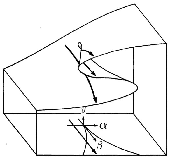
Figure 1: Cusp surface cobb1980statistical

3 Akaike information criterion

Akaike information criterion (AIC) is a model quality measure for a given data akaike1974new ; burnham2004multimodel . For a model AIC measure can be defined as follow sakamoto1986akaike ; bozdogan2000akaike :

$$AIC=-2log\mathrm{L}(\widehat{\theta})+2k,$$ (5)

where $\mathrm{L}(\widehat{\theta})$ is the maximized likelihood function and $k$ is the number of free parameters in the model. The smaller value of AIC shows that data is the better fit to model. In the proposed algorithm, we used the reverse value of AIC for ranking the features in our data.

4 The feature selection algorithm

In the Catastrophe theory, small change in certain parameters of a system can cause equilibria to appear or disappear thom1983mathematical ; zeeman1977catastrophe . We used this characteristic of the Catastrophe model to find the features that are more affective in regression analysis. In the proposed algorithm the features that better change the dynamic of outcome feature or features are considered as informative features. Assume that we are given a data set $A$ with $N$ features that $z$ is outcome feature. The algorithm takes each feature $i$ from the data set and considers it as bifurcation variable in the Cusp Catastrophe model. If this variable affects the dynamic of the system (outcome feature), it is the informative feature. The AIC value of the Cusp model is computed for each feature for ranking. The ranking of a feature $i$ can be formulated as follows:

$$AIC_{i}=AIC(-V(y;\alpha,i)),$$ (6)

where $V$ is the potential function for the Cusp model (see Equation 3), $AIC_{i}$ is the AIC value of the Cusp model for the feature $i$ as bifurcation value ($\beta$) and $\alpha$ is the asymmetric value in the Cusp model. Figure 2 shows the preparing the input parameters for Cusp model where the outcome feature is considered as the state variable and the features $i$ and the last features are considered as bifurcation and asymmetric values, respectively. The state variable and control values can be computed as follows grasman2009fitting :

$$y[t]=w[0]+w[1]*Y[t,1]+...+w[p]*Y[t,p],$$ (7)

$$\alpha[t]=a[0]+a[1]*X[t,1]+...+a[p]*X[t,p],$$ (8)

$$\beta[t]=b[0]+b[1]*X[t,1]+...+b[p]*X[t,p],$$ (9)

where $X[t,p]$’s are independent and $Y[t,p]$’s are dependent features in the data set. The vectors $a[j]$’s, $b[j]$’s and $w[j]$’s are estimated by means of maximum likelihood. The rank of each feature $i$ in the data set can be calculated as follows:

$$rank_{i}\leftarrow\frac{1}{AIC_{i}}.$$ (10)

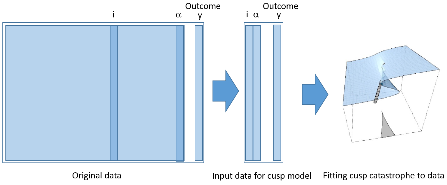
Figure 2: Preparing input features for Cusp Catastrophe model

More details about the model are shown in the Algorithm 1.

Algorithm 1 Feature selection algorithm based on the Cusp Catastrophe model and AIC ranking

1:(Initialization) $N\leftarrow$ Number of features ,$N_{F}\leftarrow$ Number of informative features , $\alpha\leftarrow feature_{N}$, $i\leftarrow 1$ and $\alpha$ is asymmetric variable

2: Let $\beta\leftarrow feature_{i}$ be bifurcation value in the Cusp model

3: (Fitting the Cusp model using $\alpha$ and $\beta$) Let $AIC_{i}$ be the Akaike information criterion value of the fitting Cusp model using parameters $\alpha$ and $\beta$

4: (Ranking the feature) $rank_{i}\leftarrow\frac{1}{AIC_{i}}$ is the rank of feature $i$ in the dataset

5: if $\frac{1}{AIC_{i}}\leq t$ then $feature_{i}$ is not informative and eliminate it, $i\leftarrow i+1$ and go to 6

6: (Stopping criterion) if $i>N_{F}$ stop. Otherwise go to Step 2

7: (Retraining informative features) Return $N_{F}$ informative features.

Here $N$ is the number of all feature in the data set and $N_{F}$ ($N_{F}<N$) is the number of informative features. For all features $i$ of the data set their rank in the data set is computed ($rank_{i}$). The set of informative features with $N_{F}$ features is the outcome of the algorithm.

5 RELIEF feature selection algorithm

Next, we give a brief description of the RELIEF algorithm. More detailed description can be found in Kira1992 ; Kononenko1994 ; Robnik-Sikonja1997 . For a given data set with $m$ samples, and threshold of relevancy $\tau$ ($0\leq\tau\leq 1$), it detects those features which are statistically relevant to the target concept ($Y=f(X)$). Differences of feature value between two instances $X$ and $Y$ are defined by the following function $diff$ kira1992feature .

$$diff(x_{k},y_{k})=(x_{k}-y_{k})/nu_{k},$$ (11)

where $nu_{k}$ is a normalization unit to normalize the values of $diff$ into the interval $[0,l]$. RELIEF picks a sample composed of $m$ triplets of an instance $X$, it’s same-class instance ($nearHit$) and closest different-class instance ($nearMiss$). RELIEF uses the $p$-dimensional Euclidean distance for selecting $nearHit$ and $nearMiss$. In every routine the feature weight $W$ vector is updated as follows:

$$W_{i}=W_{i-1}-(x_{i}-nearHit_{i})^{2}+(x_{i}-nearMiss_{i})^{2}.$$ (12)

Then the average feature weight vector relevance is determined for every sample triple. Finally, it chooses the features whose average weight is above the given threshold $\tau$.

6 Experimental results

The effectiveness of the proposed algorithm is verified using three different data sets: Parkinson’s Telemonitoring, Breast Cancer and Slice locality from UCI machine learning repository blake1998uci . Numerical experiments have been carried out on a PC with Processor Intel(R) Core(TM) i5-3470S CPU 2.90 GHz and 8 GB RAM running under Windows 7.
In numerical experiments we apply the proposed algorithm to find a ranking sequence of features in data sets. Then we apply different regression analysis algorithms from WEKA to compute regression error with subsets of features. The following regression analysis algorithms from WEKA are used in numerical experiments:

• Linear regression: Linear regression finds the best curve to fit the data by computing the relationship between a scalar dependent variable $y$ and one or more explanatory variables denoted $X$. It applies least squares, which minimizes the sum of the distance from the line for each of points. The actual observations, $y_{i}$, may be slightly off the population line because of variability in the population. The equation is $y_{i}=\beta_{0}+\beta_{1}x_{i}+\epsilon_{i}$, where $\epsilon_{i}$ is the deviation from the population line which is called the residual barlow1993numerical ; neter1983applied .

• K nearest neighbors regressor: The algorithm computes the mean of the function values of its $K$-nearest neighbours kramer2011unsupervised .

• M5Rulles: It generates rules for numeric prediction by separate-and-conquer and at each iteration builds a model tree using M5 and makes the ”best” leaf into a rule Holmes1999 ; Quinlan1992 ; Wang1997

• REPTree: Reptree is a fast tree learner that uses reduced error pruning witten2005data .

6.1 Results for Breast cancer data set

Breast Cancer Wisconsin (Prognostic) Data Set contains 30 features with 569 samples. Each record represents follow-up data for one breast cancer case mangasarian1995breast ; street1995inductive . Table 1 presents the error of analysing the data using for regression analysis algorithms. The second row shows the number of features before and after feature selection. Results from this table demonstrate that features selected by the proposed algorithm allow us to reduce the mean absolute error (MAE) regression. MAE is calculated as follows:

$$MAE=\frac{1}{n}\sum_{i=1}^{n}\left|f_{i}-y_{i}\right|,$$ (13)

where $n$ is the number of observation, $f_{i}$ is the predicted and $y_{i}$ is the true values. Although this data set is not noisy the proposed algorithm is able to significantly reduce the number of features without deteriorating the regression error. Regression errors with the subsets of features which are better than that of for all features are presented in bold font.

Table 1: Performance of regression analysis algorithms for breast cancer data set

	Original data	After feature selection
Number of features	30	25	20	15	10	6	5
Linear Regression	0.003	0.003	0.003	0.003	0.003	0.003	0.004
IBK	0.008	0.008	0.008	0.007	0.007	0.006	0.007
M5P	0.003	0.003	0.003	0.003	0.003	0.003	0.004
M5Rules	0.003	0.003	0.003	0.003	0.003	0.003	0.004

6.2 Results for Slice locality data set

Slice locality data set consists of 384 features extracted from 53500 CT images. The CT images are from 74 different patients (43 male, 31 female). The class variable of this data set is the location of the CT slice on the axial axis of the human body graf20112d . This data set is available on UCI Machine Learning Repository.

Results for 10 subjects of Slice locality data set are presented in Tables 2-5. In these tables regression error obtained by regression algorithms are given. The second line in all tables contains a number of features of original data and after feature selection. Table 2 presents results for all subjects using IBK algorithm. One can see that the IBK algorithm achieved the better accuracy for all subjects data set except subject number 10 using 380 features. Table 3 presents results for all subjects using Logistic regression algorithm. The use of the proposed algorithm allows improving the performance of Logistic regression using 250 features for Subject 1 and 150 features for Subjects 2 and 3. The best performance for Subject 5 achieved using 100 features. Results are almost the same for other Subjects.

Tables 4 and 5 show results for all patients using M5P and M5Rules algorithms, respectively. Results for these two algorithms are very similar and one can see that the proposed algorithm can improve the accuracy of regression algorithms.

Table 2: IBK algorithm performance for 10 subjects from Slice locality data

	Original data	After feature selection
Number of features	385	380	350	300	250	200	150	100
Patient1	0.059	0.059	0.059	0.060	0.061	0.065	0.063	0.083
Patient2	0.080	0.080	0.081	0.081	0.082	0.083	0.085	0.103
Patient3	0.076	0.076	0.076	0.075	0.076	0.077	0.086	0.115
Patient4	0.060	0.060	0.060	0.061	0.062	0.063	0.066	0.081
Patient5	0.078	0.078	0.078	0.079	0.080	0.088	0.086	0.090
Patient6	0.349	0.349	0.349	0.349	0.336	0.346	0.456	0.466
Patient7	0.081	0.081	0.081	0.081	0.081	0.087	0.091	0.099
Patient8	0.087	0.087	0.087	0.087	0.086	0.086	0.093	0.099
Patient9	0.364	0.364	0.370	0.370	0.364	0.380	0.494	0.516
Patient10	0.098	0.098	0.100	0.104	0.103	0.105	0.110	0.139

Table 3: Logistic regression algorithm performance for 10 subjects from Slice locality data

	Original data	After feature selection
Number of features	385	380	350	300	250	200	150	100
Patient1	0.354	0.392	0.250	0.267	0.284	0.326	0.411	0.570
Patient2	0.496	0.435	0.398	0.367	0.332	0.309	0.376	0.621
Patient3	0.258	0.256	0.266	0.228	0.226	0.226	0.247	0.361
Patient4	0.282	0.294	0.305	0.281	0.294	0.269	0.373	0.476
Patient5	0.928	1.742	2.413	0.512	0.440	0.469	0.572	0.529
Patient6	0.435	0.439	0.456	0.440	0.456	0.572	2.232	1.514
Patient7	0.515	0.500	0.460	0.426	0.420	0.414	0.443	0.756
Patient8	1.306	1.272	1.275	1.275	1.449	1.234	1.457	2.025
Patient9	0.549	0.539	0.567	0.532	0.497	0.860	1.857	7.839
Patient10	0.570	0.565	0.513	0.522	0.508	0.492	0.506	0.681

Table 4: M5P algorithm performance for 10 subjects from Slice localization data

	Original data	After feature selection
Number of features	385	380	350	300	250	200	150	100
Patient1	0.299	0.299	0.301	0.297	0.294	0.293	0.298	0.338
Patient2	0.455	0.455	0.440	0.443	0.441	0.471	0.451	0.452
Patient3	0.352	0.352	0.352	0.349	0.358	0.343	0.342	0.337
Patient4	0.341	0.347	0.348	0.350	0.339	0.310	0.319	0.325
Patient5	0.458	0.458	0.427	0.404	0.395	0.375	0.385	0.396
Patient6	1.334	1.297	1.289	1.326	1.357	1.136	1.229	1.291
Patient7	0.472	0.467	0.472	0.472	0.469	0.476	0.475	0.490
Patient8	0.782	0.797	0.801	0.801	0.720	0.744	0.728	0.728
Patient9	1.214	1.214	1.175	1.189	1.152	1.020	1.683	1.754
Patient10	0.561	0.546	0.542	0.513	0.513	0.519	0.509	0.519

Table 5: M5Rules algorithm performance for 10 subjects for Slice localization data

	Original data	After feature selection
Number of features	385	380	350	300	250	200	150	100
Patient1	0.331	0.319	0.313	0.368	0.370	0.322	0.272	2.217
Patient2	0.455	0.455	0.360	0.339	0.347	0.557	0.445	0.490
Patient3	0.508	0.508	0.508	0.477	0.432	0.413	0.388	0.420
Patient4	0.328	0.307	0.311	0.328	0.333	0.294	0.309	0.317
Patient5	0.481	0.479	0.410	0.507	0.508	0.458	0.492	0.412
Patient6	1.562	1.320	1.231	1.313	1.338	1.030	1.480	1.242
Patient7	0.783	0.783	0.784	0.783	0.559	0.500	0.412	0.611
Patient8	0.686	0.687	0.696	0.696	0.853	0.822	0.755	2.506
Patient9	1.476	1.476	1.220	1.249	1.162	1.260	0.968	1.952
Patient10	0.815	0.693	0.727	0.714	0.688	-	1.926	0.586

6.3 Results for Parkinsons Telemonitoring data set

In this paper, we present the results for Parkinsons Telemonitoring data set. This data set composed of a range of biomedical voice measurements from 42 people with early-stage Parkinson’s disease. Here we analyzed 15 subjects from this data set. Results for subjects of Parkinsons Telemonitoring data set are presented in Tables 6-9. This is illustration of a number of features in original data and after feature selection. The number of features in original data is 18.
Table 6 shows the results for the error of the data using IBK regressor algorithm. The use of a very small subset of features can provide better performance for almost all subjects. Table 7 presents the results for Logistic regression algorithm. The proposed algorithm can reduce the error of more than 70% of cases. The situation is almost the same for the M5P algorithm 8, but M5Rulles algorithm provides better performance and the accuracy is increased for all subjects except Subjects 14 and 15.

Table 6: IBK algorithm performance for Parkinson’s disease data

	Original data	After feature selection
Number of features	18	11	10	9	8	7	6	5	4
Subject1	0.037	0.038	0.037	0.038	0.038	0.040	0.044	0.041	0.042
Subject2	0.039	0.037	0.039	0.038	0.039	0.040	0.036	0.040	0.042
Subject3	0.030	0.027	0.027	0.027	0.027	0.026	0.029	0.027	0.027
Subject4	0.039	0.034	0.034	0.035	0.035	0.036	0.034	0.035	0.037
Subject5	0.037	0.033	0.032	0.032	0.030	0.029	0.029	0.030	0.031
Subject6	0.034	0.037	0.035	0.033	0.033	0.033	0.031	0.031	0.031
Subject7	0.040	0.033	0.033	0.034	0.030	0.034	0.035	0.036	0.035
Subject8	0.032	0.031	0.033	0.034	0.032	0.033	0.036	0.036	0.036
Subject9	0.041	0.038	0.038	0.039	0.039	0.037	0.036	0.036	0.039
Subject10	0.044	0.037	0.039	0.039	0.044	0.046	0.044	0.042	0.040
Subject11	0.022	0.022	0.022	0.021	0.021	0.021	0.020	0.021	0.023
Subject12	0.030	0.024	0.024	0.028	0.029	0.030	0.032	0.032	0.030
Subject13	0.040	0.042	0.044	0.042	0.047	0.039	0.051	0.049	0.049
Subject14	0.032	0.030	0.030	0.031	0.031	0.031	0.031	0.033	0.033
Subject15	0.032	0.031	0.030	0.030	0.032	0.031	0.030	0.032	0.032

Table 7: Linear regression algorithm performance for Parkinson’s disease data

	Original data	After feature selection
Number of features	18	11	10	9	8	7	6	5	4
Subject1	0.030	0.028	0.028	0.028	0.028	0.028	0.028	0.029	0.029
Subject2	0.028	0.028	0.030	0.031	0.030	0.030	0.030	0.030	0.030
Subject3	0.018	0.019	0.018	0.020	0.020	0.020	0.022	0.021	0.021
Subject4	0.029	0.028	0.027	0.027	0.027	0.027	0.027	0.027	0.028
Subject5	0.024	0.025	0.025	0.025	0.025	0.026	0.026	0.026	0.027
Subject6	0.024	0.025	0.024	0.025	0.025	0.025	0.025	0.025	0.025
Subject7	0.024	0.024	0.024	0.023	0.023	0.024	0.024	0.024	0.025
Subject8	0.027	0.031	0.035	0.034	0.034	0.034	0.033	0.031	0.034
Subject9	0.029	0.029	0.030	0.030	0.030	0.030	0.037	0.037	0.038
Subject10	0.033	0.033	0.033	0.033	0.032	0.032	0.032	0.032	0.034
Subject11	0.017	0.017	0.016	0.016	0.016	0.016	0.016	0.017	0.017
Subject12	0.019	0.018	0.017	0.021	0.021	0.021	0.020	0.020	0.021
Subject13	0.031	0.030	0.031	0.030	0.032	0.033	0.033	0.033	0.035
Subject14	0.024	0.020	0.019	0.019	0.019	0.020	0.020	0.020	0.027
Subject15	0.019	0.020	0.018	0.018	0.018	0.018	0.021	0.021	0.022

Table 8: M5P algorithm performance for Parkinson’s disease data

	Original data	After feature selection
Number of features	18	11	10	9	8	7	6	5	4
Subject1	0.030	0.028	0.028	0.028	0.028	0.028	0.029	0.029	0.029
Subject2	0.027	0.028	0.029	0.030	0.030	0.030	0.030	0.030	0.030
Subject3	0.018	0.019	0.018	0.020	0.020	0.020	0.022	0.021	0.021
Subject4	0.028	0.027	0.027	0.027	0.025	0.027	0.027	0.027	0.028
Subject5	0.024	0.023	0.023	0.023	0.023	0.022	0.022	0.023	0.024
Subject6	0.025	0.025	0.024	0.025	0.025	0.025	0.025	0.025	0.025
Subject7	0.024	0.024	0.024	0.023	0.023	0.024	0.023	0.024	0.025
Subject8	0.024	0.026	0.029	0.029	0.030	0.030	0.029	0.030	0.030
Subject9	0.029	0.029	0.028	0.028	0.029	0.029	0.031	0.031	0.031
Subject10	0.034	0.034	0.034	0.034	0.032	0.032	0.032	0.032	0.032
Subject11	0.017	0.017	0.016	0.016	0.016	0.016	0.016	0.017	0.017
Subject12	0.020	0.018	0.017	0.021	0.021	0.021	0.020	0.020	0.021
Subject13	0.033	0.031	0.031	0.031	0.032	0.033	0.033	0.033	0.035
Subject14	0.019	0.019	0.019	0.019	0.019	0.021	0.020	0.020	0.023
Subject15	0.019	0.021	0.019	0.019	0.019	0.019	0.023	0.023	0.022

Table 9: M5Rules algorithm performance for Parkinson’s disease data

	Original data	After feature selection
Number of features	18	11	10	9	8	7	6	5	4
Subject1	0.030	0.028	0.029	0.029	0.028	0.028	0.029	0.029	0.029
Subject2	0.027	0.029	0.029	0.031	0.030	0.030	0.030	0.030	0.030
Subject3	0.019	0.019	0.018	0.020	0.020	0.021	0.022	0.021	0.021
Subject4	0.029	0.028	0.028	0.027	0.026	0.028	0.030	0.030	0.028
Subject5	0.025	0.023	0.023	0.023	0.023	0.022	0.022	0.023	0.024
Subject6	0.024	0.025	0.024	0.025	0.025	0.025	0.025	0.025	0.025
Subject7	0.024	0.024	0.024	0.023	0.023	0.025	0.024	0.024	0.025
Subject8	0.029	0.038	0.043	0.043	0.031	0.031	0.044	0.045	0.031
Subject9	0.031	0.030	0.029	0.029	0.030	0.031	0.032	0.032	0.031
Subject10	0.035	0.035	0.035	0.034	0.033	0.033	0.033	0.033	0.033
Subject11	0.017	0.017	0.016	0.016	0.016	0.016	0.016	0.017	0.017
Subject12	0.019	0.018	0.017	0.021	0.021	0.021	0.020	0.020	0.021
Subject13	0.033	0.031	0.031	0.031	0.032	0.033	0.033	0.033	0.035
Subject14	0.019	0.020	0.020	0.019	0.019	0.021	0.020	0.020	0.023
Subject15	0.020	0.021	0.020	0.020	0.020	0.020	0.023	0.024	0.022

Figure 3 demonstrates applying different classifiers for Parkinson’s disease data set. Figure 3 indicates that cusp model is reduced the error of classifiers for almost all subjects from Parkinson’s disease data set.

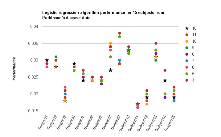
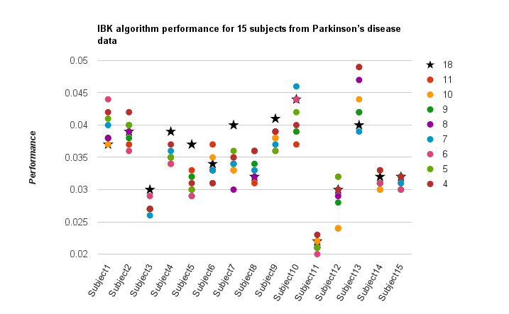
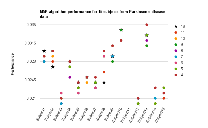
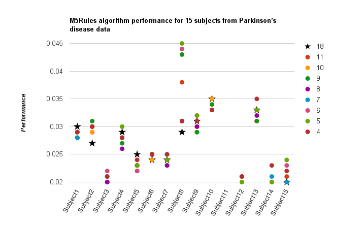
Figure 3: Classification algorithms performance for Parkinson’s disease data using all features and after feature selection using cusp catastrophe feature selection algorithm

Figures 4 show the Equilibrium surface (3 dimensional) and control surface (2 dimensional) of fitting the most irrelevant (left) and the most significant features in different data sets using the Cusp Catastrophe model. The informative features have more affect on the system and put the system closer to the bifurcation situation.

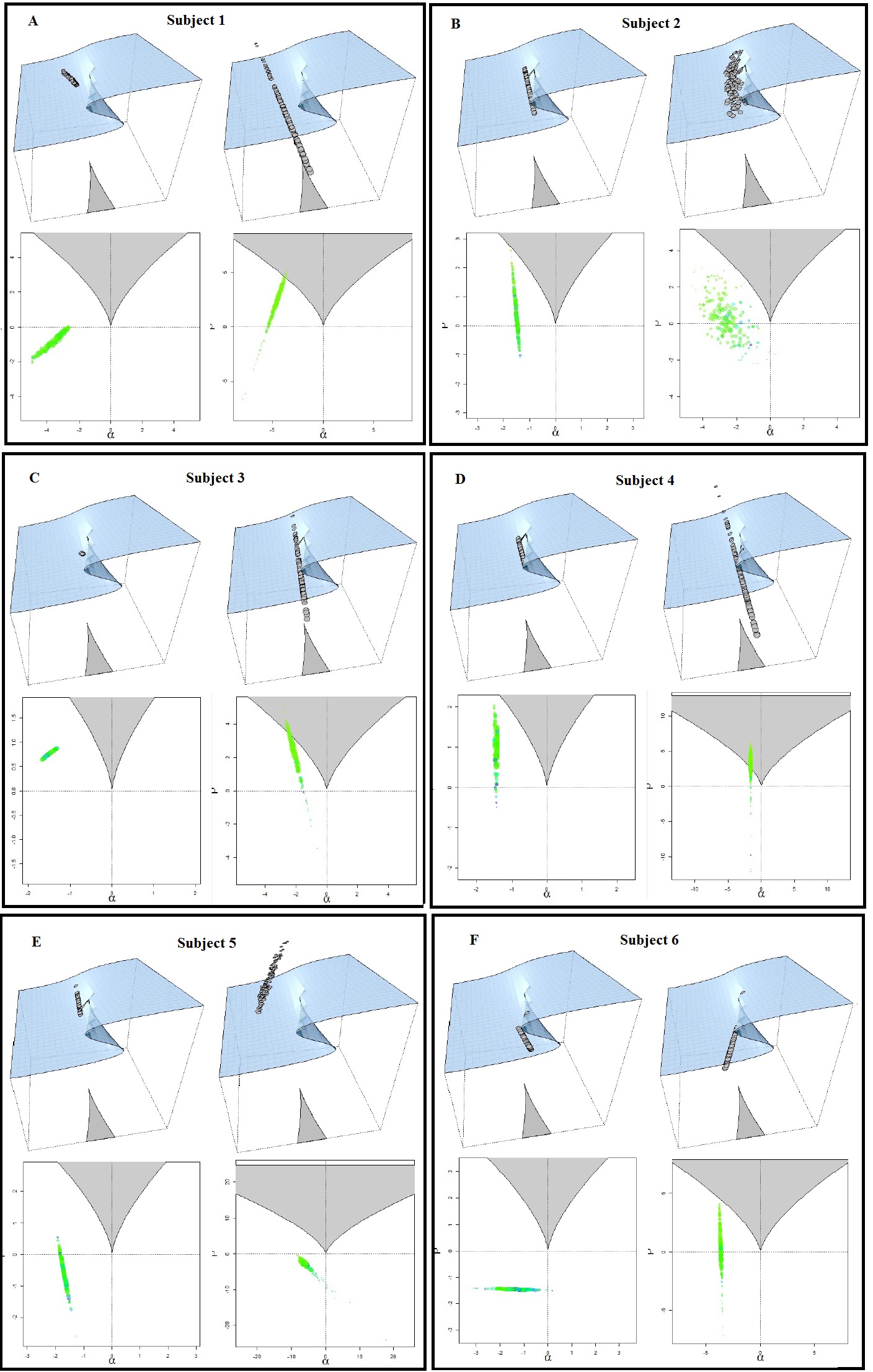
Figure 4: Cusp plot: The most least informative features (left) and the most least informative features (right) base on proposed algorithm for subject 1 to subject 6

Tables 10- 15 show the ranking of the features using the proposed and RELIEF algorithms. The ranking values are not exactly the same, but the for almost all cases the informative features’ levels are similar in both ranking results. For example, for the first subject, the informative features of 3, 14, 4 and 6 are in the top of the table in both algorithms and less-significant features 2 and 17 are at the bottom.

Table 10: Ranking of the features using the proposed and RELIEF algorithms for subject 1 from Parkinson’s disease data

Feature selection algorithm based on the Cusp model		RELIEF algorithms
Attribute ID	Rank	Attribute ID	Rank
3	0.003144	14	0.030901
14	0.003096	3	0.014302
4	0.003052	6	0.014158
6	0.002947	4	0.011554
15	0.002923	5	0.009576
5	0.002732	7	0.009572
7	0.002731	15	0.006487
9	0.002685	12	0.004949
12	0.002586	16	0.004764
16	0.002569	9	0.004034
8	0.002565	11	0.001722
11	0.002564	13	0.0016
10	0.0025	10	0.001595
13	0.0025	2	0.000525
17	0.002358	8	-0.00004
2	0.002351	1	-0.00254
1	0.002351	17	-0.00378

Table 11: Ranking of the features using the proposed and RELIEF algorithms for subject 2 from Parkinson’s disease data

Feature selection algorithm based on the Cusp model		RELIEF algorithms
Attribute ID	Rank	Attribute ID	Rank
16	0.003336	14	0.0195
6	0.003299	6	0.00943
14	0.003241	16	0.00907
9	0.003212	12	0.00784
12	0.0032	9	0.00706
4	0.003173	3	0.00582
3	0.003167	4	0.00309
15	0.003154	15	0.003
8	0.003134	11	0.0026
13	0.003069	13	0.00244
10	0.003069	10	0.00244
11	0.003057	7	0.00243
7	0.00304	5	0.00242
5	0.00304	8	0.0023
2	0.002727	2	0.00133
1	0.002727	1	0.00107
17	0.002718	17	-0.00237

Table 12: Ranking of the features using the proposed and RELIEF algorithms for subject 3 from Parkinson’s disease data

Feature selection algorithm based on the Cusp model		RELIEF algorithms
Attribute ID	Rank	Attribute ID	Rank
15	0.003585	15	0.024669
6	0.003473	14	0.018446
3	0.003261	6	0.016579
4	0.003031	3	0.013203
14	0.002994	4	0.010286
7	0.002946	5	0.007498
9	0.002946	7	0.00748
5	0.002945	11	0.005778
12	0.002937	12	0.003904
8	0.002934	9	0.00329
11	0.002933	1	0.003219
10	0.00287	8	0.002655
13	0.002869	10	0.002304
16	0.002627	13	0.002297
1	0.002595	17	0.002161
2	0.002589	2	0.000729
17	0.002565	16	-0.00093

Table 13: Ranking of the features using the proposed and RELIEF algorithms for subject 4 from Parkinson’s disease data

Feature selection algorithm based on the Cusp model		RELIEF algorithms
Attribute ID	Rank	Attribute ID	Rank
3	0.004621	6	0.02566
4	0.00456	3	0.02124
6	0.004473	17	0.01921
5	0.003827	4	0.01823
7	0.003826	14	0.01734
14	0.003417	5	0.01714
15	0.003254	7	0.01711
9	0.002984	2	0.00843
8	0.002968	15	0.00774
13	0.002935	13	0.00711
10	0.002935	10	0.00711
12	0.00293	11	0.00695
11	0.00291	12	0.00676
17	0.002904	8	0.00671
16	0.002793	9	0.00613
1	0.002771	1	0.00519
2	0.00277	16	0.00168

Table 14: Ranking of the features using the proposed and RELIEF algorithms for subject 5 from Parkinson’s disease data

Feature selection algorithm based on the Cusp model		RELIEF algorithms
Attribute ID	Rank	Attribute ID	Rank
14	0.003896	14	0.02979
3	0.003671	6	0.02661
4	0.003533	4	0.02327
6	0.003529	3	0.01819
7	0.003189	7	0.01289
5	0.003185	5	0.01287
15	0.003059	9	0.01101
16	0.00253	15	0.0101
9	0.00248	12	0.00659
12	0.002401	11	0.00414
8	0.002372	10	0.00354
11	0.002363	13	0.00354
10	0.002343	8	0.00331
13	0.002343	16	0.00278
2	0.002339	2	0.00244
1	0.002324	17	0.00116
17	0.002314	1	-0.00406

Table 15: Ranking of the features using the proposed and RELIEF algorithms for subject 6 from Parkinson’s disease data

Feature selection algorithm based on the Cusp model		RELIEF algorithms
Attribute ID	Rank	Attribute ID	Rank
15	0.003297	14	0.014851
4	0.003173	6	0.014336
3	0.003093	15	0.014142
6	0.003076	17	0.01388
14	0.003062	4	0.012454
7	0.002854	3	0.010648
5	0.002854	7	0.008541
9	0.002691	5	0.008525
12	0.002649	2	0.003976
8	0.002644	12	0.002502
11	0.002619	1	0.001973
16	0.002597	11	0.001794
10	0.002565	9	-6.8E-05
13	0.002565	8	-0.0006
1	0.002418	13	-0.00153
2	0.00234	10	-0.00153
17	0.002315	16	-0.00244

Tables 16-23 show the mean absolute error and root mean square error for Regression analysis before and after feature selection for 15 subjects. We separated the results of different algorithms from each other. Tables 16 and 17 shows the results of Linear regression algorithm. The accuracy of analyzing all subjects except subject 2, 9 and 14 using the proposed algorithm compared with original data is improved. The RELIEF algorithm has improvement for almost all subjects, but our algorithm has better performance than RELIEF algorithm.

Tables 18-19 are the related results for K-nearest neighbors algorithm and they show that both algorithms have better accuracy only for 60% of subjects and the same situation happened for M5Rulles (see the tables 20-21) and REPTree (22-23) algorithms, but for some subjects the RELIEF algorithm has better performance.

Table 16: Mean absolute error of Linear regression algorithm after feature selection using the proposed and RELIEF algorithms for Slice locality data set

	MAE of Linear Regression
Subject	Original data	After Feature selection using feature selection algorithm based on the Cusp model	After feature selection using RELIEF algorithms
1	0.0295	0.0291	0.0282
2	0.0276	0.028	0.028
3	0.0183	0.0183	0.0182
4	0.0292	0.029	0.0292
5	0.0235	0.0235	0.0235
6	0.0239	0.0239	0.024
7	0.0243	0.0242	0.0244
8	0.0266	0.0266	0.028
9	0.0286	0.0288	0.0288
10	0.0333	0.0333	0.0333
11	0.0169	0.0167	0.017
12	0.0193	0.0187	0.0194
13	0.0305	0.0297	0.0315
14	0.019	0.0193	0.0188
15	0.0266	0.0261	0.0266

Table 17: Root mean square error of Linear regression algorithm after feature selection using the proposed and RELIEF algorithms for Slice locality data set

	RMSE of Linear Regression
Subject	Original data	After Feature selection using feature selection algorithm based on the Cusp model	After feature selection using RELIEF algorithm
1	0.0386	0.0381	0.0384
2	0.0372	0.0377	0.0377
3	0.0249	0.0249	0.0248
4	0.042	0.0418	0.042
5	0.0336	0.0336	0.0336
6	0.0325	0.0325	0.0322
7	0.0338	0.0338	0.0335
8	0.0401	0.0401	0.0424
9	0.0376	0.0377	0.0375
10	0.0472	0.0472	0.0461
11	0.0239	0.0237	0.024
12	0.025	0.0245	0.0256
13	0.0404	0.0392	0.0425
14	0.0248	0.0253	0.0246
15	0.0322	0.0317	0.0319

Table 18: Mean absolute error of IBK algorithm after feature selection using the proposed and RELIEF algorithms for Slice locality data set

	MAE of IBK
Subject	Original data	After Feature selection using feature selection algorithm based on the Cusp model	After feature selection using RELIEF algorithm
1	0.037	0.038	0.042
2	0.0389	0.0411	0.0411
3	0.0304	0.0297	0.0311
4	0.0394	0.0387	0.0372
5	0.0369	0.0344	0.0356
6	0.034	0.0334	0.0355
7	0.0404	0.0385	0.0389
8	0.0321	0.032	0.032
9	0.0405	0.0399	0.0399
10	0.0439	0.044	0.0433
11	0.0218	0.0231	0.0224
12	0.0297	0.0295	0.0308
13	0.0402	0.0411	0.0402
14	0.0317	0.03	0.0307
15	0.0338	0.0352	0.0335

Table 19: Root mean square error of IBK algorithm after feature selection using the proposed and RELIEF algorithms for Slice locality data set

	RMSE of IBK
Subject	Original data	After Feature selection using feature selection algorithm based on the Cusp model	After feature selection using RELIEF algorithm
1	0.0493	0.0506	0.0548
2	0.0526	0.0537	0.0537
3	0.0379	0.0379	0.0401
4	0.0569	0.0565	0.0567
5	0.0499	0.047	0.0477
6	0.0453	0.0447	0.0457
7	0.0527	0.0504	0.0507
8	0.0462	0.0458	0.0466
9	0.0531	0.0528	0.0536
10	0.056	0.0562	0.0538
11	0.0285	0.0316	0.029
12	0.0385	0.0399	0.0402
13	0.0533	0.0539	0.0532
14	0.038	0.0359	0.0378
15	0.0426	0.0435	0.0427

Table 20: Mean absolute error of M5Rules algorithm after feature selection using the proposed and RELIEF algorithms for Slice locality data set

	MAE of M5Rules
Subject	Original data	After Feature selection using feature selection algorithm based on the Cusp model	After feature selection using RELIEF algorithm
1	0.0299	0.0299	0.0292
2	0.0273	0.0285	0.0276
3	0.0188	0.0181	0.0203
4	0.0291	0.0291	0.0278
5	0.0246	0.0248	0.0233
6	0.0241	0.024	0.024
7	0.0237	0.0233	0.0235
8	0.0286	0.0275	0.0262
9	0.0306	0.0319	0.0306
10	0.0349	0.0349	0.034
11	0.0167	0.0169	0.0175
12	0.019	0.0188	0.0197
13	0.0333	0.0313	0.032
14	0.0196	0.021	0.0209
15	0.0246	0.0249	0.0256

Table 21: Root mean square error of M5Rules algorithm after feature selection using the proposed and RELIEF algorithms for Slice locality data set

	RMSE of M5Rules
Subject	Original data	After Feature selection using feature selection algorithm based on the Cusp model	After feature selection using RELIEF algorithm
1	0.0393	0.0393	0.0393
2	0.0366	0.0377	0.0366
3	0.0259	0.0252	0.0284
4	0.0423	0.0423	0.0415
5	0.0343	0.0345	0.0318
6	0.0327	0.0327	0.0327
7	0.033	0.0324	0.0328
8	0.0457	0.0444	0.0388
9	0.0403	0.0424	0.0401
10	0.0488	0.0488	0.0478
11	0.0219	0.0225	0.0235
12	0.0244	0.0244	0.026
13	0.044	0.041	0.0424
14	0.0258	0.0286	0.0275
15	0.0305	0.0305	0.0314

Table 22: Mean absolute error of REPTree algorithm after feature selection using the proposed and RELIEF algorithms for Slice locality data set

	MAE of REPTree
Subject	Original data	After Feature selection using feature selection algorithm based on the Cusp model	After feature selection using RELIEF algorithm
1	0.0357	0.0357	0.0353
2	0.0344	0.0347	0.0347
3	0.0223	0.0228	0.0226
4	0.0312	0.0308	0.0304
5	0.0272	0.0273	0.0276
6	0.0278	0.028	0.0278
7	0.0273	0.0276	0.0276
8	0.03	0.0311	0.03
9	0.0387	0.0381	0.0387
10	0.0358	0.0358	0.0349
11	0.0183	0.018	0.0184
12	0.0261	0.0267	0.0261
13	0.043	0.043	0.0428
14	0.0263	0.0263	0.0263
15	0.0288	0.0289	0.0293

Table 23: Root mean square error of REPTree algorithm after feature selection using the proposed and RELIEF algorithms for Slice locality data set

	RMSE of REPTree
Subject	Original data	After Feature selection using feature selection algorithm based on the Cusp model	After feature selection using RELIEF algorithm
1	0.0458	0.0458	0.0453
2	0.0449	0.0448	0.0448
3	0.0284	0.0288	0.0288
4	0.0449	0.0446	0.0437
5	0.0363	0.0363	0.0367
6	0.0371	0.038	0.0371
7	0.0379	0.0387	0.0383
8	0.0506	0.0547	0.0506
9	0.0519	0.0513	0.052
10	0.0458	0.0458	0.0454
11	0.0251	0.025	0.0252
12	0.0336	0.0356	0.0335
13	0.0538	0.0538	0.0538
14	0.0339	0.0338	0.0339
15	0.0362	0.0363	0.0366

Figure 5 provides a comparison between proposed algorithm and the well known RELIEF algorithm for Slice locality data set. Mean absolute error and root mean square error of four classifiers of original data and after feature selection are shown in the figures. The graph show that the proposed algorithm is improved the accuracy of classification algorithms for almost all subjects using different classifiers.

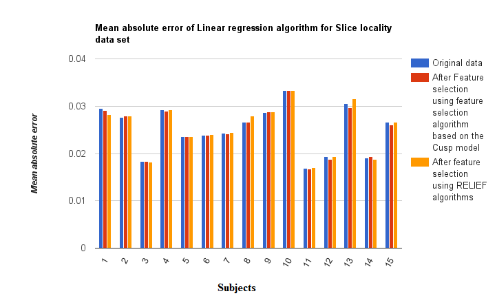
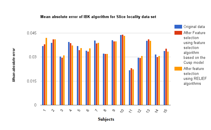
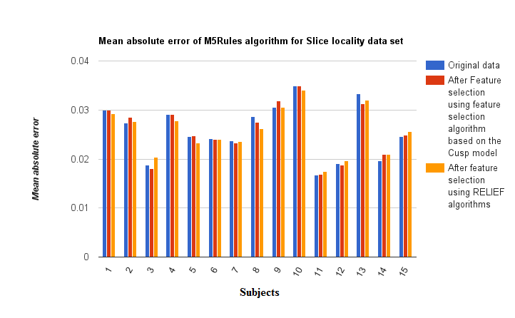
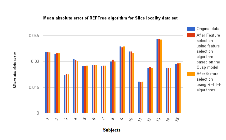
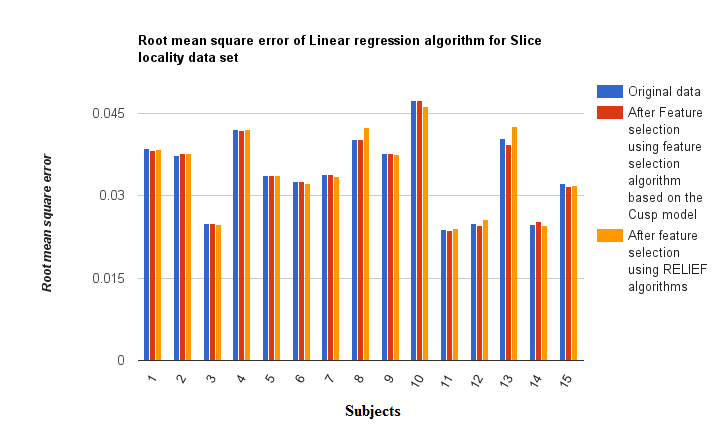
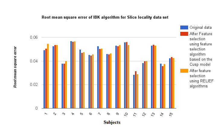
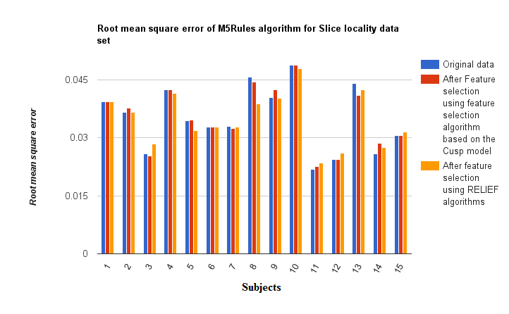
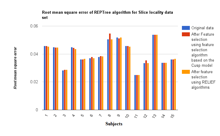
Figure 5: Mean square error and root mean square error of classifiers after feature selection using the proposed and RELIEF algorithms for Slice locality data set

7 Conclusions

In this paper, we introduced a new feature selection algorithms to remove the irrelevant or redundant features in the data sets. This algorithm removes the irrelevant or redundant features of a regression data sets. This algorithm selects significant features based on their fitting to the Catastrophe model and the features that better change the dynamics of the outcome feature or features are considered as informative features. The Akaike information criterion value of the Cusp model is computed for ranking of each feature. We applied this algorithm to three different data sets: Parkinson’s Telemonitoring, Breast Cancer and Slice locality from UCI machine learning repository. Results show that the proposed algorithm is efficient in finding the significant subset of features in a data set.

References

(1)Akaike, H.A new look at the statistical model identification.
Automatic Control, IEEE Transactions on 19, 6 (1974), 716–723.
(2)Barlow, J. L.Numerical aspects of solving linear least squares problems.
Handbook of Statistics 9 (1993), 303–376.
(3)Blake, C., and Merz, C. J.UCI repository of machine learning databases.
(4)Bozdogan, H.Akaike’s information criterion and recent developments in information
complexity.
Journal of mathematical psychology 44, 1 (2000), 62–91.
(5)Burnham, K. P., and Anderson, D. R.Multimodel inference understanding aic and bic in model selection.
Sociological methods & research 33, 2 (2004), 261–304.
(6)Cobb, L.Estimation theory for the cusp catastrophe model.
In Proceedings of the Section on Survey Research Methods
(1980), pp. 772–776.
(7)Cobb, L., and Watson, B.Statistical catastrophe theory: An overview.
Mathematical Modelling 1, 4 (1980), 311–317.
(8)Graf, F., Kriegel, H.-P., Schubert, M., Pölsterl, S., and Cavallaro,
A.2d image registration in ct images using radial image descriptors.
In Medical Image Computing and Computer-Assisted
Intervention–MICCAI 2011. Springer, 2011, pp. 607–614.
(9)Grasman, R. P., van der Maas, H. L., and Wagenmakers, E.-J.Fitting the cusp catastrophe in r: A cusp-package primer.
Journal of Statistical Software 32, 8 (2009), 1–28.
(10)Holmes, G., Hall, M., and Frank, E.Generating rule sets from model trees.
In Twelfth Australian Joint Conference on Artificial
Intelligence (1999), Springer, pp. 1–12.
(11)Kira, K., and Rendell, L. A.The feature selection problem: Traditional methods and a new
algorithm.
In AAAI (1992), pp. 129–134.
(12)Kira, K., and Rendell, L. A.A practical approach to feature selection.
In Ninth International Workshop on Machine Learning (1992),
D. H. Sleeman and P. Edwards, Eds., Morgan Kaufmann, pp. 249–256.
(13)Kononenko, I.Estimating attributes: Analysis and extensions of relief.
In European Conference on Machine Learning (1994),
F. Bergadano and L. D. Raedt, Eds., Springer, pp. 171–182.
(15)Ku, S.-p., Gretton, A., Macke, J., and Logothetis, N. K.Comparison of pattern recognition methods in classifying
high-resolution bold signals obtained at high magnetic field in monkeys.
Magnetic resonance imaging 26, 7 (2008), 1007–1014.
(16)Mangasarian, O. L., Street, W. N., and Wolberg, W. H.Breast cancer diagnosis and prognosis via linear programming.
Operations Research 43, 4 (1995), 570–577.
(17)Mourão-Miranda, J., Reynaud, E., McGlone, F., Calvert, G., and
Brammer, M.The impact of temporal compression and space selection on svm
analysis of single-subject and multi-subject fmri data.
NeuroImage 33, 4 (2006), 1055–1065.
(18)Neter, J., Wasserman, W., and Kutner, M. H.Applied linear regression models.
Irwin Homewood, IL, 1983.
(19)Norman, K., Polyn, S., Detre, G., and Haxby, J.Beyond mind-reading: multi-voxel pattern analysis of fmri data.
Trends in cognitive sciences 10, 9 (2006), 424–430.
(20)O’Toole, A. J., Jiang, F., Abdi, H., Pénard, N., Dunlop, J. P., and
Parent, M. A.Theoretical, statistical, and practical perspectives on pattern-based
classification approaches to the analysis of functional neuroimaging data.
Journal of cognitive neuroscience 19, 11 (2007), 1735–1752.
(21)Quinlan, R. J.Learning with continuous classes.
In 5th Australian Joint Conference on Artificial Intelligence
(Singapore, 1992), World Scientific, pp. 343–348.
(22)Robnik-Sikonja, M., and Kononenko, I.An adaptation of relief for attribute estimation in regression.
In Fourteenth International Conference on Machine Learning
(1997), D. H. Fisher, Ed., Morgan Kaufmann, pp. 296–304.
(23)Sakamoto, Y., Ishiguro, M., and Kitagawa, G.Akaike information criterion statistics.
Dordrecht, The Netherlands: D. Reidel (1986).
(24)Saunders, P. T.An introduction to catastrophe theory.
Cambridge University Press, 1980.
(25)Street, W. N., Mangasarian, O. L., and Wolberg, W. H.An inductive learning approach to prognostic prediction.
In ICML (1995), Citeseer, pp. 522–530.
(26)Thom, R.Mathematical models of morphogenesis.
New York (1983).
(27)Wang, Y., and Witten, I. H.Induction of model trees for predicting continuous classes.
In Poster papers of the 9th European Conference on Machine
Learning (1997), Springer.
(28)Witten, I. H., and Frank, E.Data Mining: Practical machine learning tools and techniques.
Morgan Kaufmann, 2005.
(29)Zeeman, E. C.Catastrophe theory: Selected papers, 1972–1977.Addison-Wesley, 1977.