Refining mass formulas for astrophysical applications:
a Bayesian neural network approach

Abstract

Background

Exotic nuclei, particularly those near the driplines, are at the core of one of the fundamental questions driving nuclear structure and astrophysics today: what are the limits of nuclear binding? Exotic nuclei play a critical role in both informing theoretical models as well as in our understanding of the origin of the heavy elements.

Purpose

To refine existing mass models through the training of an artificial neural network that will mitigate the large model discrepancies far away from stability.

Methods

The basic paradigm of our two-pronged approach is an existing mass model that captures as much as possible of the underlying physics followed by the implementation of a Bayesian Neural Network (BNN) refinement to account for the missing physics. Bayesian inference is employed to determine the parameters of the neural network so that model predictions may be accompanied by theoretical uncertainties.

Results

Despite the undeniable quality of the mass models adopted in this work, we observe a significant improvement (of about 40%) after the BNN refinement is implemented. Indeed, in the specific case of the Duflo-Zuker mass formula, we find that the rms deviation relative to experiment is reduced from $\sigma_{\rm rms}\!=\!0.503$ MeV to $\sigma_{\rm rms}\!=\!0.286$ MeV. These newly refined mass tables are used to map the neutron drip lines (or rather “dripbands”) and to study a few critical $r$-process nuclei.

Conclusions

The BNN approach is highly successful in refining the predictions of existing mass models. In particular, the large discrepancy displayed by the original “bare” models in regions where experimental data is unavailable is considerably quenched after the BNN refinement. This lends credence to our approach and has motivated us to publish refined mass tables that we trust will be helpful for future astrophysical applications.

I Introduction

Where do the chemical elements come from and how did they evolve is one of the central questions animating nuclear science today Lon (2015). Stars heavier than about eight solar masses ($M_{\star}\!\gtrsim\!8\,M_{\odot}$) reach high enough core temperatures to support the formation of ever-heavier chemical elements by thermonuclear fusion: from helium all the way to iron. Yet, once the iron-peak elements are synthesized, thermonuclear burning stops abruptly with the formation of an inert iron core that will collapse once its mass exceeds the Chandrasekhar limit Clayton (1983); Phillips (1998); Iliadis (2007). This situation naturally begs the question: how did the elements heavier than iron form? Whereas the slow neutron capture process (“$s$-process”) in asymptotic giant branch stars is believed to be responsible for the formation of about half of the heavy elements beyond iron (such as strontium, barium, and lead) identifying the precise site (or sites) of the rapid neutron capture process (“$r$-process”) responsible for the remaining half of of the heavy elements (such as gold, platinum, and uranium) remains elusive Burbidge et al. (1957); Clayton (1983); Wallerstein et al. (1997). Indeed, “How were the elements from iron to uranium made?” has been identified as one of the eleven science questions for the new century Qua (2003).

Understanding $r$-process nucleosynthesis is a fascinating and challenging multidisciplinary problem. Progress in this area demands detailed knowledge of a host of nuclear-structure observables—often at the limits of nuclear existence—such as masses, neutron capture rates, and nuclear beta decays Burbidge et al. (1957); Petermann et al. (2010); Mumpower et al. (2016). Given that the $r$-process develops under extreme astrophysical conditions such as those found in the merger of two neutron stars, neutron capture on seed nuclei occurs on a time scale that is much faster than the competing beta-decay rates. This drives the $r$-process far away from stability where little is known about the thousands of exotic nuclear species that participate in these reactions; see Refs. Wallerstein et al. (1997); Petermann et al. (2010); Mumpower et al. (2016) and references contained therein. In an effort to mitigate this problem, Mumpower and collaborators have performed sensitivity studies to identify the nuclear inputs (e.g., nuclear masses) that have the greatest impact on the $r$-process Mumpower et al. (2016, 2015a, 2015b). Whereas these studies suggest that some of the “most influential” nuclear masses are within reach of future radioactive beam facilities, it is also recognized that some others will likely remain beyond experimental reach. Hence, theoretical guidance becomes absolutely critical. Unfortunately, theoretical mass models that agree in the vicinity of measured nuclear masses, disagree strongly—often by several MeV—far away from stability. This is particularly troublesome given that some sensitivity studies suggest that resolving the abundance pattern will require reducing mass-model uncertainties to $\lesssim\!100$ keV Mumpower et al. (2015b).

The emergence of the $r$-process pattern is highly sensitive to nuclear masses in the vicinity of neutron magic numbers $N\!=\!50,82$, and $126$. Interestingly, nuclear masses around closed shells $N\!=\!50$ and $82$ also have a profound impact on the composition of a different astrophysical system: the outer crust of a neutron star. Given that at the low densities of relevance to the outer crust ($10^{4}$ – $10^{11}\,{\rm g/cm^{3}}$) the average inter-nucleon separation is considerably larger than the range of the nuclear interaction, it becomes energetically favorable for nucleons to cluster into individual nuclei that arrange themselves in a crystalline lattice that is immersed in a uniform free Fermi gas of electrons Baym et al. (1971). And whereas the underlying dynamics is relatively simple, the exotic composition of the outer stellar crust is also highly sensitive to nuclear masses in regions where experimental information is not yet available Roca-Maza and Piekarewicz (2008). Thus, as in the case of the $r$-process, understanding the composition of the stellar crust relies heavily on theoretical extrapolations into unknown regions of the nuclear chart.

In an effort to lessen the impact of such inevitable extrapolations we have recently intoduced a Bayesian Neural Network (BNN) approach for the calculation of nuclear masses Utama et al. (2016a); Piekarewicz and Utama (2016) and charge radii Utama et al. (2016b). The novel framework proposed in Ref. Utama et al. (2016a) consists of a combined scheme that relies on accurate theoretical predictions that are subsequently refined by training a suitable artificial neural network on the residuals between the experimental data and the theoretical predictions. In essence, the central tenet of our approach is to include as much physics as possible in the underlying nuclear model and then rely on a BNN refinement to recover most of the physics that is missing from the model. In our earlier work we were able to identify several virtues of such combined approach. First, by using a randomly selected set of experimentally known masses to train the neural network, we observed a significant improvement in the predictions of the remaining known masses that were not included in the training set—even for some of the most sophisticated mass models available in the literature. Second, it is well known that theoretical mass models of similar quality agree in regions where masses are known, but differ widely (by as much as tens of MeVs) in regions where experimental data is not yet available Blaum (2006). However, after implementing the BNN refinement we found that the large differences in the model predictions were significantly reduced. Finally, given the “Bayesian” character of the approach, the refined predictions were accompanied by properly estimated theoretical errors Utama et al. (2016a).

In our earlier work we have successfully tested the BNN paradigm in the context of nuclear masses of relevance to the outer crust of neutron stars Utama et al. (2016a); Piekarewicz and Utama (2016). It is the main goal of the present paper to provide updated mass tables that encompass the entire nuclear chart. As several sophisticated and successful mass tables already exist Möller and Nix (1981, 1988); Möller et al. (1995); Duflo and Zuker (1995); Goriely et al. (2010); Kortelainen et al. ; Erler et al. (2013), the initial phase of our program—namely, the selection of an underlying model that incorporates as much physics as possible—is essentially complete. Thus, the remaining task is to implement the BNN refinement on these highly successful models. Our hope is that the BNN refinement will improve the original mass models by reducing the large systematic uncertainties and by providing realistic statistical errors. Together with the publication of these updated mass tables, we will also make available (with associated theoretical uncertainties) related observables that may be more suitable for certain astrophysical applications, such as one- and two-nucleon separation energies. It is our hope that these tables will contribute to further our understanding of astrophysical phenomena as well as to constrain theoretical models of nuclear structure. Ultimately, of course, any progress in theory is strongly coupled to experimental advances. Indeed, we are at the dawn of a new era where rare isotope facilities will probe the limits of nuclear existence and in so doing will provide critical guidance to theoretical models. And although some of the required theoretical extrapolations will take us far into regions of the nuclear chart that are unlikely to be explored even at the most sophisticated facilities, measurements of even a few exotic short-lived isotopes are of critical importance for the improvement of theoretical models.

The manuscript has been organized as follows. In the next section we provide some additional details on the strong synergy between nuclear structure and astrophysics. As the BNN approach has been presented elsewhere Utama et al. (2016a), we limit the discussion on the formalism to a brief outline of the method and its implementation in Sec. III. Next, in Sec. IV we focus on the improvement to several existing mass models after the BNN refinement. Only in the case of the 10-parameter version of the Duflo-Zuker mass model Duflo and Zuker (1995) we recalibrate the parameters in order to extract the associated covariance matrix that encodes statistical uncertainties and correlations among the model parameters. In this way the overall theoretical error will have its origin in two sources: (a) the uncertainty in calibration of the “bare” model parameters and (b) the errors emerging from the BNN refinement. Also presented in this section are results for proton and neutron drip lines as well as a few masses of particular relevance to the $r$-process. Finally, we conclude in Sec. V with a summary of our important findings.

II Astrophysical Motivation

Although of fundamental and high intrinsic nuclear-physics value, modern nuclear mass tables find today their best expression in astrophysical applications. In particular, nuclear masses are of paramount importance in understanding nucleosynthesis in hot stellar environments and the crustal composition of cold neutron stars. In what follows we provide a brief description of these two scenarios underscoring the critical role of nuclear masses far away from equilibrium.

II.1 Neutron capture and photo-dissociation: $(\gamma,n)$ equilibrium

Although modern $r$-process simulations make no assumptions on whether stellar conditions—such as temperature, density, and neutron fraction—are favorable to maintain the reaction $(n,\gamma)\!\rightleftharpoons\!(\gamma,n)$ in thermodynamic equilibrium, the outcome of such network calculations suggests that under many astrophysical scenarios equilibrium is indeed attained, at least during the early stages. Under such an astrophysical scenario, the final abundance pattern follows solely from statistical equilibrium and nuclear physics. In particular, the pattern along a given isotopic chain is set by the temperature ($T$), the neutron density ($N_{n}$), and the one-neutron separation energy ($S_{n}$). In essence, once thermodynamic equilibrium has been established in a given astrophysical environment, the final abundance pattern along an isotopic chain is entirely determined by nuclear masses, both near and far from the valley of stability. The ratio of yields of neighboring isotopes at equilibrium is set by the equality of the chemical potential of the competing species. Given that $\mu_{\gamma}\!\equiv\!0$ one obtains,

$$\mu(Z,A)+\mu_{n}=\mu(Z,A+1).$$ (1)

In the limit of low neutron density and high temperature, so that each component may be treated as a classical ideal gas, the condition of chemical equilibrium is encoded in the Saha equation Clayton (1983); Phillips (1998); Iliadis (2007):

$$\frac{Y(Z,A+1)}{Y(Z,A)}=\frac{G(Z,A+1)}{2G(Z,A)}N_{n}\lambda_{n}^{3}(T)\exp\!\left(\frac{S_{n}(Z,A+1)}{k_{B}T}\right).$$ (2)

Here $Y(Z,A)$ and $G(Z,A)$ denote the isotopic abundance and partition function of the seed nucleus, and $\lambda_{n}(T)\!=\!\sqrt{2\pi/m_{n}k_{\rm B}T}$ is the de Broglie thermal wavelength of the neutron. Often $N_{Q}\!=\!\lambda^{-3}_{n}(T)$ is referred to as the quantum concentration; if $N_{n}\!\ll\!N_{Q}$ then the system behaves classically. The nuclear dynamics is imprinted in the neutron separation energy

$$S_{n}(Z,A+1)\!\equiv\!M(Z,A)+m_{n}-M(Z,A+1)=B(Z,A+1)-B(Z,A),$$ (3)

with $B(Z,A)$ the total nuclear binding energy. Note that the relative abundance is exponentially sensitive to errors in the neutron separation energy. For example, at a canonical stellar temperature of $T_{9}\!=\!10^{9}\,{\rm K}$, a relatively “modest” error in the separation energy of $0.1$ MeV translates into an error in the relative abundance of about a factor of three. Eventually, chemical equilibrium is lost and the final abundance pattern is dictated by a series of $\beta$ decays back to stability. Here too nuclear masses are of critical importance since the phase-space factor for beta decay is determined by the reaction $Q$-value: $Q_{\beta}\!=\!M(Z,A)\!-\!M(Z+1,A)$.

II.2 Crustal composition of a neutron star

Another powerful connection between astrophysics and nuclear physics that is highly sensitive to nuclear masses involves the crustal composition of a neutron star, particularly its outer crust Baym et al. (1971); Haensel et al. (1989); Haensel and Pichon (1994); Ruester et al. (2006); Roca-Maza and Piekarewicz (2008); Roca-Maza et al. (2011). The crust is interesting because the dynamics is simple yet subtle. Simple, because nuclear masses is the only ingredient driving the composition of the outer crust. Subtle, since the crustal composition emerges from a delicate dynamics between the electronic energy and the nuclear symmetry energy. Indeed, at the densities of relevance to the outer crust, it is energetically favorable for nucleons to cluster into nuclei that arrange themselves in a body-centered cubic lattice that itself is immersed in a neutralizing electron background Baym et al. (1971). At zero temperature and fixed pressure, the dynamics of the outer crust is encoded in the following expression for the chemical potential (or Gibbs free energy per nucleon) of the system:

$$\mu(Z,A;P)=\frac{M(Z,A)}{A}+\frac{Z}{A}\mu_{e}-\frac{4}{3}C_{l}\frac{Z^{2}}{A^{4/3}}\,p_{{}_{\rm F}}.$$ (4)

The first term—which is independent of the pressure—depends exclusively on the mass per nucleon of the “optimal” nucleus populating the crystal lattice. The second term $\mu_{e}$ is the chemical potential of a relativistic Fermi gas of electrons. Finally, the last term provides the relatively modest, although by no means negligible, lattice contribution ($C_{l}\!=\!3.40665\!\times\!10^{-3}$) to the chemical potential. Note that both the electronic

$$\mu_{e}\!=\!\sqrt{\left(\frac{Z}{A}\right)^{\!\!2/3}p_{\rm F}^{2}+m_{e}^{2}}\,,$$ (5)

and lattice contributions have been written in terms of the Fermi momentum $p_{{}_{\rm F}}=(3\pi^{2}n)^{1/3}$ (or equivalently the baryon density $n$) rather than the pressure. The connection between the baryon density and the pressure is obtained through the equation of state. That is Roca-Maza and Piekarewicz (2008),

$$P(Z,A;n)=\frac{m_{e}^{4}}{3\pi^{2}}\left(x_{{}_{\rm F}}^{3}y_{{}_{\rm F}}-\frac{3}{8}\left[x_{{}_{\rm F}}y_{{}_{\rm F}}\Big{(}x_{{}_{\rm F}}^{2}+y_{{}_{\rm F}}^{2}\Big{)}-\ln(x_{{}_{\rm F}}+y_{{}_{\rm F}})\right]\right)-\frac{n}{3}C_{l}\frac{Z^{2}}{A^{4/3}}\,p_{{}_{\rm F}},$$ (6)

where

$$x_{{}_{\rm F}}\!=\!\frac{p^{(e)}_{{}_{\rm F}}}{m_{e}}=\left(\frac{Z}{A}\right)^{1/3}\!\frac{p_{{}_{\rm F}}}{m_{e}}\quad{\rm and}\quad y_{{}_{\rm F}}\!=\!\sqrt{1\!+\!x_{{}_{\rm F}}^{2}}\,,$$ (7)

are the scaled electronic Fermi momentum and Fermi energy, respectively. Given that the outer crust spans nearly seven orders of magnitude in density, from about $10^{4}{\rm g/cm^{3}}$ to $10^{11}{\rm g/cm^{3}}$, changes in the nuclear composition with density (or pressure) are interesting despite the simplicity of the underlying dynamics. For example, at the top of the outer crust where the pressure is low and so is the density, the electronic contribution to the chemical potential is negligible, so it is favorable to populate the crystal lattice with the nucleus having the the lowest mass per nucleon in the entire nuclear chart: ⁵⁶Fe. However, as the pressure and the density increase, it becomes energetically advantageous for the system to lower its electron fraction $Y_{e}\!=\!Z/A$ via electron capture on the protons. As a consequence, ⁵⁶Fe ceases to be the optimal nucleus due to the presence of a uniform sea of neutralizing electrons whose chemical potential increases rapidly with density. Thus, the essential physics of the outer crust involves a competition between an electronic contribution that favors $Y_{e}\!=\!0$ and the nuclear symmetry energy that instead favors $Y_{e}\!\simeq\!1/2$.

Ultimately, computing the nuclear composition of the stellar crust requires precise knowledge of nuclear masses over three well-defined regions of the nuclear chart. At the top of the crust the electronic contribution to the chemical potential is small to moderate, so the isotopes of relevance are located around the stable iron-nickel region where nuclear masses are very well known. As the proton fraction becomes too low and the symmetry energy large, it becomes energetically favorable for the system to jump into the $N\!=\!50$ region. The nuclei of relevance in this region lie at the boundary between those whose masses are accurately known (e.g., ⁹⁰Zr, ⁸⁸Sr, and ⁸⁶Kr) and those that are poorly known (such as ⁷⁸Ni). We should mention that until very recently the mass of ⁸²Zn was not known. Yet, the mass of ⁸²Zn was determined fairly recently at the ISOLDE-CERN facility, leading to an interesting modification of the crustal composition Wolf et al. (2013). Finally, the third region comprising the bottom layers of the outer crust requires knowledge of nuclear masses at the $N\!=\!82$ shell closure. Depending on the particular mass model, the nuclei of relevance span the region from ¹³²Sn ($Z\!=\!50$) all the way down to ¹¹⁸Kr ($Z\!=\!36$) Roca-Maza et al. (2011). For this region theoretical extrapolations are unavoidable as little or no experimental information is available Utama et al. (2016a). Indeed, ¹¹⁸Kr is 21 neutrons away from the last measured isotope with a well measured mass Wang et al. (2012a).

III Formalism

III.1 Bayesian neural networks

The novel theoretical approach that we advocate here aims to refine some existing mass models through a BNN approach Neal (1996). Given the proven success of modern mass models, the BNN refinement is implemented by training a suitable neural network on the residuals between the experimental data and the “bare” (i.e., before refinement) theoretical predictions. Our ultimate goal is to generate a universal approximator Cybenko (1989); Hornik et al. (1989); that is, a neural network that can provide an “educated” extrapolation into unexplored regions of the nuclear chart with properly quantified theoretical uncertainties. A detailed description of the origins and development of Bayesian neural networks goes beyond the scope of this paper; for a detailed exposition see Refs. Neal (1996); Bishop ; Haykin ; Vapnik . Thus, as we have done elsewhere Utama et al. (2016a); Piekarewicz and Utama (2016); Utama et al. (2016b), we limit ourselves to highlight the main features of the approach. Before we do so, however, we note that the idea of using artificial neural networks in nuclear physics—mainly to estimate unknown properties of exotic nuclei of relevance to astrophysics—started in the early 90s with the work of Clark and collaborators Gazula et al. (1992); Gernoth et al. (1993); Gernoth and Clark (1995); Clark et al. (1999) and continues up to this day Athanassopoulos et al. (2004, 2006); Clark and Li (2006); Costiris et al. (2009); Bayram et al. (2014) with more sophisticated applications.

Statistical inference based on Bayes’ theorem—as applied in this work—connects two critical pieces of information: (a) a prior hypothesis reflecting beliefs that one has acquired through experience or previous empirical information and (b) an improvement to the prior hypothesis by both adopting and adapting new evidence (e.g., experimental data). In this context Bayes’ theorem may be written as Stone (2013):

$$p(\omega|x,t)=\frac{p(x,t|\omega)p(\omega)}{p(x,t)},$$ (8)

where $p(\omega)$ is the prior distribution of the model parameters $\omega$ and $p(x,t|\omega)$ is the “likelihood” that a given model $\omega$ describes the new evidence $t(x)$. The product of the prior and the likelihood form the posterior distribution $p(\omega|x,t)$ that encodes the probability that a given model describes the data $t(x)$. In essence, the posterior represents the improvement to $p(\omega)$ as a result of the new evidence $p(x,t|\omega)$. Note that the “marginal likelihood” $p(x,t)$ is independent of the model parameters $\omega$, so for our purposes it may be regarded as an overall normalization factor. To define the likelihood we start by introducing an objective (or cost) function in terms of a least-squares fit to the empirical data. That is,

$$\chi^{2}(\omega)=\sum_{i=1}^{N}\left(\frac{t_{i}-f(x_{i},\omega)}{\Delta t_{i}}\right)^{2},$$ (9)

where $N$ is the total number of data points, $t_{i}\!\equiv\!t(x_{i})$ is the empirical value of the target evaluated at the $i$th input $x_{i}$, $\Delta t_{i}$ is the associated error, and the universal approximator $f(x,\omega)$ depends on both the input data and the model parameters $\omega$; see Eq.(11) below. From such an objective function the likelihood is customarily defined as

$$p(x,t|\omega)=\exp\big{(}\!-\!\chi^{2}(\omega)/2\big{)}.$$ (10)

In the particular case of interest here, i.e., nuclear masses, the input $x\!\equiv\!(Z,A)$ represents the charge and mass number of the nucleus and $t(x)\!\equiv\!\delta M(Z,A)$ the mass residual between the experimental data and the theoretical predictions. Note that maximizing the likelihood $p(x,t|\omega)$ provides the maximum likelihood estimation of the model parameters.

The neural network function $f(x,\omega)$ adopted here has the following “sigmoid” form:

$$f(x,\omega)=a+\sum_{j=1}^{H}b_{j}\tanh\left(c_{j}+\sum_{i=1}^{I}d_{ji}x_{i}\right),$$ (11)

where the model parameters (or “connection weights”) are collectively given by $\omega\!=\!\big{\{}a,b_{j},c_{j},d_{ji}\big{\}}$, $H$ is the number of hidden nodes, and $I$ is the number of inputs. The “universal approximation theorem” states that such a neural network can accurately represent a wide variety of functions; $\tanh$ is a common form of the sigmoid activation function that controls the firing of the artificial neurons Cybenko (1989); Hornik et al. (1989). See Fig. 1 for a simple depiction of a feed-forward neural network consisting of a single hidden layer with three nodes.

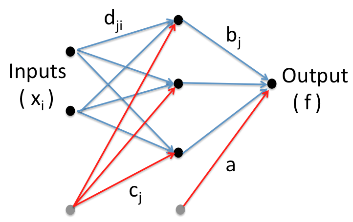
Figure 1: An example of a feed-forward neural network with a single hidden layer consisting of three nodes. In our case, the two inputs that define the nucleus of interest are $Z$ and $A$, and a single output provides an estimate of $\delta M(Z,A)$, namely, the discrepancy between the bare theoretical prediction and the experimental value.

Given the complexity of the posterior distribution $p(\omega|x,t)$, we adopt Markov Chain Monte Carlo (MCMC) sampling to generate a faithful equilibrium distribution. Once a significant number of samples has been generated, reliable estimates for both the average and variance of $\delta M(Z,A)$ are obtained. That is,

$$\langle f_{n}\rangle =\frac{1}{K}\sum_{k=1}^{K}f(x_{n},\omega_{k}),$$ (12a)

$$\langle f^{2}_{n}\rangle =\frac{1}{K}\sum_{k=1}^{K}f^{2}(x_{n},\omega_{k}),$$ (12b)

$$\Delta f_{n} =\sqrt{\langle f_{n}^{2}\rangle-\langle f_{n}\rangle^{2}},$$ (12c)

where $x_{n}\!=\!(Z_{n},A_{n})$ represents a particular nucleus with charge $Z_{n}$ and mass number $A_{n}$, $K$ is the total number of Monte Carlo configurations, and $f(x_{n},\omega_{k})$ is the neural network estimate of $\delta M(Z_{n},A_{n})$ as predicted by the $k$th Monte Carlo configuration.

Finally, we conclude this section by briefly addressing the choice of prior $p(\omega)$ assumed in this work. Prior probabilities encode our beliefs concerning the model parameters and are an essential ingredient of the Bayesian paradigm. Normally, the prior is highly informative as it is based on our own physics biases and intuition, which are often well informed by prior experimental data. Unfortunately, whereas physics principles guide the construction of modern nuclear mass models, physics intuition is of no help in designing the connection weights $\omega$. Thus, we are forced to rely on assumptions that have been proven effective and reliable through mostly trial and error Neal (1996). Following our earlier work Utama et al. (2016a), we assume all connection weights to be independent and adopt a Gaussian prior centered around zero and with a width determined as in Ref. Neal (1996). For an extensive discussion on the determination of the “hyperparameters” controlling the width of the Gaussian prior see Refs. MacKay (1995, 1999).

IV Results

The aim of this section is to discuss the improvement to three successful mass models as a result of the BNN refinement. The three models under consideration are: (i) the 10-parameter Duflo-Zuker model (DZ10) Mendoza-Temis et al. (2010), (ii) the 28-parameter Duflo-Zuker model (DZ) Duflo and Zuker (1995), and (iii) the microscopic Hartree-Fock-Bogoliubov model (HF19) of Ref. Goriely et al. (2010). In all three cases the predictions after refinement have the distinct advantage of being accompanied by theoretical uncertainties. However, for the simpler DZ10 model we found instructive to re-calibrated the model-parameters, as this process generates a suitable covariance matrix from where statistical uncertainties and correlation coefficients may be computed. To reiterate, the basic paradigm of our two-pronged approach is to start with a robust underlying mass model that captures as much physics as possible followed by a BNN refinement that will hopefully account for the missing physics Utama et al. (2016a).

IV.1 The 10-parameter Duflo-Zuker Model

The original Duflo-Zuker model containing a total of 28 parameters has stood the test of time Duflo and Zuker (1995). The DZ model, fitted to the set of existing nuclear masses appearing in the 1995 compilation by Audi and collaborators Audi and Wapstra (1995), was enormously successful in predicting the more than 300 additional masses that appeared in the later AME03 compilation Audi et al. (2002). Indeed, the success of the DZ model in accurately reproducing the masses of the more than 3,000 nuclei presently known is truly remarkable Wang et al. (2012b). However, despite its undeniable success, the underlying physics of the model remains puzzling and difficult to unravel. The simpler 10-parameter Duflo-Zuker model was conceived with the sole purpose of illuminating the physics. A detailed study of DZ10 that aims to understand and possibly to also improve the model has been carried out recently by Mendoza-Temis, Hirsch, and Zuker Mendoza-Temis et al. (2010). Even more recently, Doboszewski and Szpak have refitted DZ10 with the goal of quantifying the model uncertainties and the correlations among the model parameters Doboszewski (2014).

We also proceed here by recalibrating the model parameters following closely Ref. Doboszewski (2014). To do so we start by constructing a likelihood function defined in terms of the square differences between the DZ10 predictions and the experimental binding energies provided by the AME2012 compilation Wang et al. (2012a); we limit ourselves to the ⁴⁰Ca to ²⁴⁰U region. For the initial distribution of model parameters we use an uninformative prior. In this way we generate a posterior probability distribution that is generated through Markov-Chain Monte Carlo (MCMC) sampling. Simulating such a posterior distribution is computationally inexpensive so we could afford generating one million Monte Carlo configurations, with the first 10,000 steps used for thermalization. To avoid correlations among subsequent configurations, we found that an autocorrelation “time” of about 20 configurations was sufficient. Overall, we used nearly 50,000 configurations to generate the correlation plot depicted in Fig. 2 together with the average values and uncertainties listed in Table 1. For comparison, also included in Table 1 are the results reported in Refs. Mendoza-Temis et al. (2010); Doboszewski (2014).

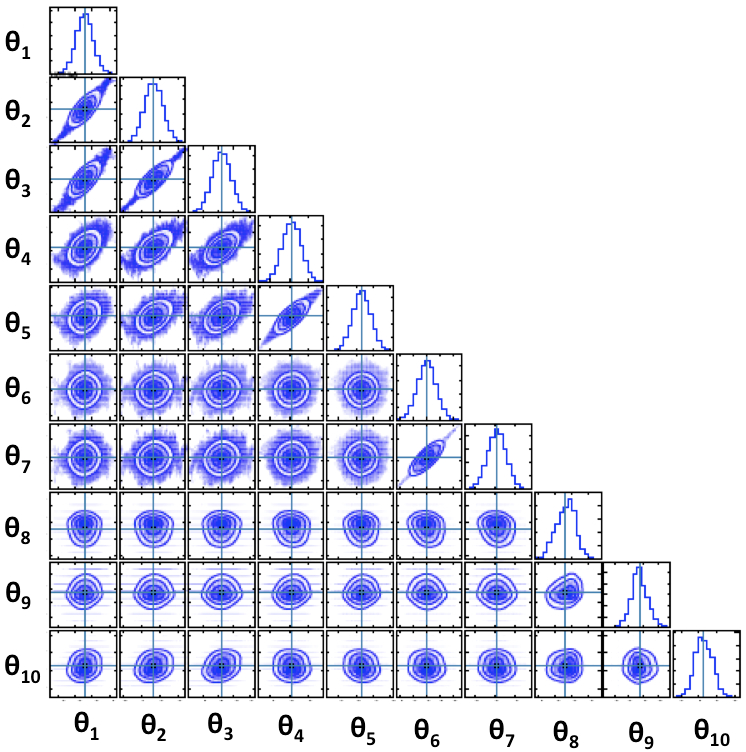
Figure 2: Correlations coefficients and marginalized probability densities (shown along the diagonal) for the 10-parameter Duflo-Zuker model Duflo and Zuker (1995); Mendoza-Temis et al. (2010); Doboszewski (2014).

Parameter	Ref Mendoza-Temis et al. (2010)	Ref. Doboszewski (2014)	This work
$\theta_{1}\!=\!a_{3}$	0.707	0.70506(37)	0.70452(27)
$\theta_{2}\!=\!a_{1}$	17.766	17.749 (70)	17.7466(49)
$\theta_{3}\!=\!a_{2}$	16.314	16.267(2)	16.277(17)
$\theta_{4}\!=\!a_{4}$	37.515	37.465(4)	37.608(27)
$\theta_{5}\!=\!a_{5}$	53.351	53.23(19)	54.08(11)
$\theta_{6}\!=\!a_{7}$	0.478	0.4631(58)	0.4601(63)
$\theta_{7}\!=\!a_{8}$	2.183	2.101(30)	2.088(33)
$\theta_{8}\!=\!a_{9}$	0.022	0.02144(17)	0.02106(19)
$\theta_{9}\!=\!a_{10}$	41.338	41.5310(2)	41.50(22)
$\theta_{10}\!=\!a_{6}$	6.199	6.238(89)	6.455(81)
$\sigma$ (MeV)	0.554	0.571	0.552

Table 1: Average values and uncertainties for the 10-parameter Duflo-Zuker model Duflo and Zuker (1995). Comparisons are made against similar results presented in Ref. Mendoza-Temis et al. (2010) (without uncertainties) and Ref. Doboszewski (2014). Here $\sigma$ represents the root-mean-square deviation of the predictions relative to the AME2012 compilation Wang et al. (2012b).

Once the theoretical predictions from the DZ10 model—or indeed any other mass model—have been generated, the BNN refinement proceeds by separating the available experimental data into two disjoint sets: a learning and a validation set. Again, to avoid regions of the nuclear landscape where the masses fluctuate too rapidly (as in the case of the lightest nuclei) we limit the experimental data set to the 2,000-plus well measured nuclei between ⁴⁰Ca and ²⁴⁰U. The learning set consists of a randomly-selected subset of nuclei contained within the experimental database that will be used to train the neural network, namely, to calibrate the connection weights as defined in Eq.(11). On the other hand, the validation set comprises the remaining nuclei that, while still in the existent experimental database, were not used in the training of the network. Thus, the validation set provides the testbed for assessing the quality of the artificial neural network. If the test is successful, then one re-calibrates the network parameters using the entire experimental database in order to predict the masses of nuclei that have not yet been measured, yet are essential for astrophysical applications. Given that the limits of nuclear binding is one of the key science driver animating nuclear science today Erler et al. (2012), besides generating refined mass tables we also provide tables for one- and two-nucleon separation energies:

$$S_{n}(Z,N) \equiv M(Z,N-1)+m_{n}-M(Z,N)=B(Z,N)-B(Z,N-1),$$ (13a)

$$S_{p}(Z,N) \equiv M(Z-1,N)+m_{p}-M(Z,N)=B(Z,N)-B(Z-1,N),$$ (13b)

$$S_{2n}(Z,N) \equiv M(Z,N-2)+2m_{n}-M(Z,N)=B(Z,N)-B(Z,N-2),$$ (13c)

$$S_{2p}(Z,N) \equiv M(Z-2,N)+2m_{p}-M(Z,N)=B(Z,N)-B(Z-2,N).$$ (13d)

All these BNN-improved tables are generated from the same ensemble of Monte Carlo configurations, so that theoretical uncertainties may be reliably attached to each individual prediction.

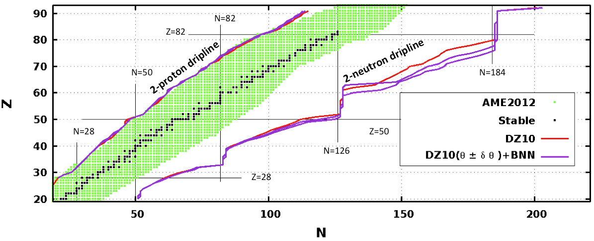
Figure 3: Proton and neutron drip lines as predicted by both the bare and BNN-refined 10-parameter Duflo-Zuker (DZ10) model. In the case of the BNN predictions, the neutron drip line evolves into a “drip band” due to statistical uncertainties. Also shown (with green points) is the AME2012 data set Wang et al. (2012a) with the stable nuclei displayed with black points.

The calibration of the neural network is computationally expensive. With two input variables ($Z$ and $N$) and a “canonical” number of $H\!=\!40$ hidden nodes, a total of $1\!+\!4H\!=\!161$ parameters must be calibrated. To do so, we rely on the Flexible Bayesian Modeling package by Neal described in detail in Ref. Neal (1996). After an initial thermalization phase consisting of 500 Monte-Carlo steps, a sampling set of 100 configurations is accumulated to determine statistical averages and their associated uncertainties. As a measure of the accuracy of our predictions, we report root-mean-square (rms) deviations relative to experiment; for simplicity, the comparison is done using exclusively average values. Due to the relative simplicity of the DZ10 model, we were able to implement the BNN refinement using two different schemes. The first scheme consists of a unique set of masses obtained from the average values generated by the new DZ10 calibration—without accounting for the uncertainties in the bare model parameters. The second scheme remedies such deficiency by effectively incorporating the distribution of DZ10 model parameters depicted in Fig. 2. Such improved version is useful in assessing whether a recalibration of the bare model parameters may be necessary in other cases. Fortunately, our results suggest that, at least in the case of DZ10, this is not required. Our results indicate that whereas there is indeed a dramatic improvement in the predictions of the bare DZ10 model after the BNN refinement—from $\sigma_{\rm rms}\!=\!0.552\,{\rm MeV}$ to $\sigma_{\rm rms}\!=\!0.292\,{\rm MeV}$—no significant changes are observed when one uses the proper statistical distribution of bare DZ10 parameters; for for this latter case one obtains $\sigma_{\rm rms}\!=\!0.296\,{\rm MeV}$.

As alluded earlier, for each of the 100 Monte-Carlo configurations obtained from the BNN refinement one computes at every MC step the mass of each individual nucleus. Having generated all nuclear masses in such a way, one may then compute the mass differences required to generate one- and two-nucleon separation energies. At each MC step one proceeds in this same exact fashion, until by the end of the 100 Monte-Carlo configurations one can finally extract average values and associated theoretical uncertainties for each nuclear observable. The outcome of such a procedure is displayed in Fig. 3 for neutron and proton drip lines, identified at the point in which the two-neutron and two-proton separation energies become negative. For the case of the bare DZ10 model, the drip lines are displayed by a solid (red) line. In contrast, BNN-improved DZ10 predictions produce drip bands, as all the predictions are now accompanied by statistical uncertainties. Note that because of the Coulomb repulsion, the proton drip line is much closer to the valley of stability than the corresponding neutron drip line. Indeed, whereas the proton drip line has been experimentally established for a large number of nuclei (up to atomic number $Z\!=\!91$), the neutron drip line is only known up to $Z\!=\!8$, with ²⁴O being the heaviest known oxygen isotope that remains stable against particle decay Thoennessen (2004). Moreover, Fig. 3 displays the characteristic signature of shell closures at neutron magic numbers 50, 82, 126, and (predicts) 184. Finally, the figure encapsulates the enormous experimental challenges faced in mapping the neutron drip line. However, even if reaching the neutron drip line for heavy nuclei may not be feasible in the foreseeable future, it is essential to continue the experimental quest to properly inform theoretical models. In turn, BNN approaches as the one advocated here may guide experimental searches for those “few” critical nuclei that may reduce the large systematic uncertainty that currently plagues theoretical models.

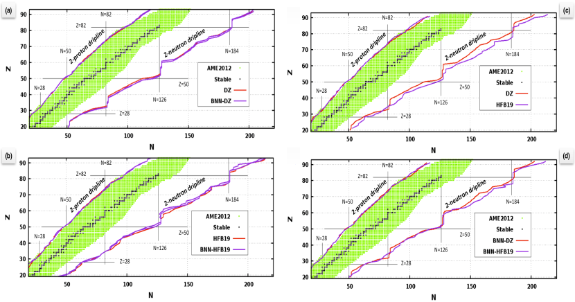
Figure 4: Proton and neutron drip lines/drip bands as predicted by (a) the Duflo-Zuker model Duflo and Zuker (1995) and (b) the HFB19 model Goriely et al. (2010); in both cases bare and BNN-refined predictions are displayed. The remaining two panels display the same information but now the comparison is between the predictions of both mass models: (c) displays bare-model results whereas (d) the corresponding ones after BNN-refinement. Also shown (with green points) is the AME2012 data set Wang et al. (2012a) with the stable nuclei displayed with black points.

So far DZ10 has provided a benchmark to quantify the impact of the BNN refinement and the role of uncertainty quantification. We found that while the BNN refinement is critical in improving the predictions of the model, there seems to be little value in propagating the uncertainties inherent to the bare model. Thus, we now proceed to document and test the predictions of the two state-of-the-art mass models that will be refined in order to generate BNN-improved tables; the 28-parameter “mic-mac” model of Duflo and Zuker Duflo and Zuker (1995) and the microscopic HFB19 model of Goriely, Chamel, and Pearson Goriely et al. (2010). Drip lines and drip bands as predicted by these two models are displayed in Fig. 4. The two left-hand panels, (a) for Duflo-Zuker and (b) for HFB19, aim to illustrate the improvement to the bare models as a result of the BNN refinement. Note that although the overall improvement to both mass models is considerable—about 40% Utama et al. (2016a)—the changes are difficult to discern because both the expanded scale as well as the intrinsic high quality of the bare models. In contrast, the two right-hand panels compare the models to each other: (c) for the bare predictions and (d) for the BNN-improved versions. In this case the improvement is clearly discernible, as the model discrepancies displayed by the bare models get significantly quenched after the BNN refinement. Indeed, at first there is an appreciable discrepancy in the predictions of the bare models—with HFB19 consistently predicting the location of the neutron drip line at larger values of $N$​. Remarkably, much of the discrepancy disappears after the BNN refinement, especially in the region between shell closures $N=82$ and $N=126$. Such reduction in the systematic model error is highly desirable and entirely consistent with the results obtained in an earlier publication Utama et al. (2016a). Moreover, we observe a significant quantitative improvement in the predictions of both models. In the case of the Duflo-Zuker mass formula the root-mean-square mass deviation improves from $\sigma_{\rm rms}\!=\!0.503$ MeV to $\sigma_{\rm rms}\!=\!0.286$ MeV, whereas in the case of HFB19 it goes from $\sigma_{\rm rms}\!=\!0.559$ MeV to $\sigma_{\rm rms}\!=\!0.358$ MeV.

We close this section with a brief discussion of the impact of the BNN refinement on a few critical $r$-process nuclei that emerge from the sensitivity study of Mumpower and collaborators Mumpower et al. (2016, 2015a, 2015b); specifically, palladium ($Z\!=\!46$), cadmium ($Z\!=\!48$), indium ($Z\!=\!49$), and tin ($Z\!=\!50$). Note that these results may be readily extended to other isotopes by employing the refined mass tables provided here as supplemental material. The main goal of our analysis is to assess whether the ubiquitous bare-model discrepancies can be systematically reduced after the implementation of the BNN refinement.

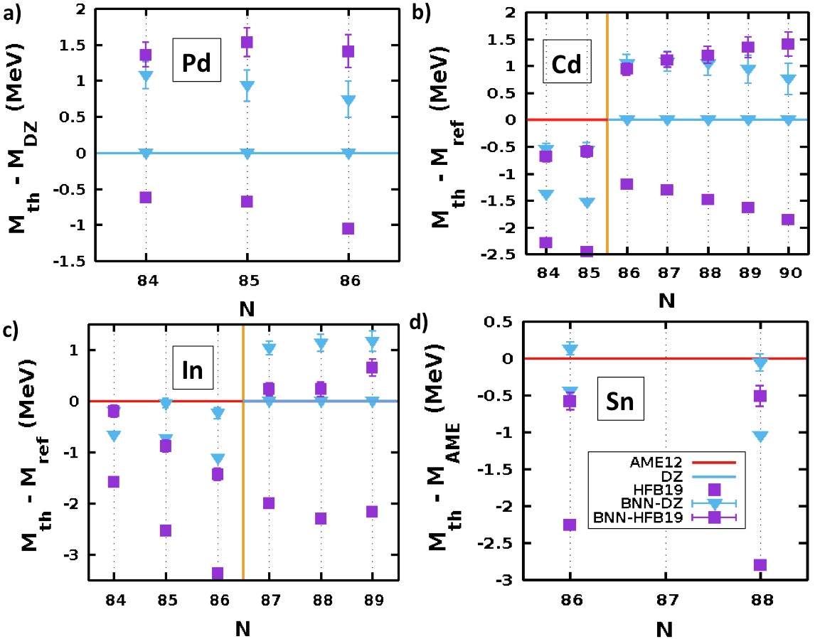
Figure 5: Mass predictions for (a) palladium ($Z\!=\!46$), (b) cadmium ($Z\!=\!48$), (c) indium ($Z\!=\!49$), and (d) tin ($Z\!=\!50$) for both the Duflo-Zuker Duflo and Zuker (1995) and HFB19 Goriely et al. (2010) mass models. The predictions are relative to a reference mass value taken from either the AME2012 compilation when available Wang et al. (2012a) or from the bare Duflo-Zuker model when unavailable. Predictions are displayed with statistical error bars for the BNN-improved models.

In Fig. 5 we display model predictions relative to a reference mass value for palladium, cadmium, indium, and tin in the region $N\!\gtrsim\!82$. The masses of all 18 nuclei displayed in the figure, ^130-132Pd, ^132-138Cd, ^133-138In, and ^136,138Sn, have been identified as important nuclei in the determination of the $r$-process abundance pattern; see Table I in Ref. Mumpower et al. (2015b). Note that the reference mass has been adopted from either “experimental” values (although derived not from purely experimental data Wang et al. (2012a)) or when data is unavailable, from the predictions of the bare Duflo-Zuker model. Theoretical predictions with error bars are from the BNN-refined models. We can state categorically that the BNN refinement has an appreciable impact in reducing the systematic model discrepancies. Easiest to visualize are the cases of palladium and tin where the number of isotopes displayed is small; three and two, respectively. For palladium there is no available experimental data so we display theoretical estimates relative to the predictions from the bare Duflo-Zuker model (depicted by the light-blue line). Whereas the bare HFB19 predictions hover around 0.5-1 MeV relative to such a baseline, the model discrepancy narrows considerably after the BNN refinement. Indeed, for ¹³⁰Pd the predictions are now consistent with each other and for the most unfavorable case of ¹³⁰Pd they agree at the 2$\sigma$ level. For tin the situation is similar, although in this case we display with a red line the recommended experimental values Wang et al. (2012a). Once again, we note that the bare-model predictions differ significantly from each other and, especially in the case of HFB19, from the recommended AME2012 values. However, once the BNN refinement is completed, both the model discrepancy is significantly reduced and the comparison with experiment is much more favorable. Indeed, both BNN-DZ predictions are now fully consistent with experiment. Finally, the two remaining isotopes of cadmium and indium display the same trends observed so far. In particular, note that for all of these 18 important nuclei the BNN refinement suggest an increase in the value of the mass, or equivalently, a reduction in the binding energy. For these two larger isotopic chains—having seven and six important nuclei, respectively—experimental mass values do exist but only for the smaller values of $N$. Yet regardless of whether experimental masses are available, we see the model spread diminishes considerably after the BNN refinement. And when recommended mass values exist, the BNN predictions are practically consistent with experiment. The isotopic chain in cadmium contains the largest number of important $r$-process nuclei. As we have learned from earlier studies (see for example Refs. Blaum (2006); Erler et al. (2012); Mumpower et al. (2015a)) bare-model discrepancies diverge dramatically as one moves away from measured mass values. This is evident in Fig. 5b where the bare-model discrepancy becomes as large as $\sim\!2$ MeV for ¹³⁸Cd (i.e., $N=90$). Remarkably, all model discrepancies are largely eliminated after the BNN refinement. In particular, even for the least favorable case of ¹³⁸Cd the 1$\sigma$ mismatch gets reduced to merely $130$ keV.

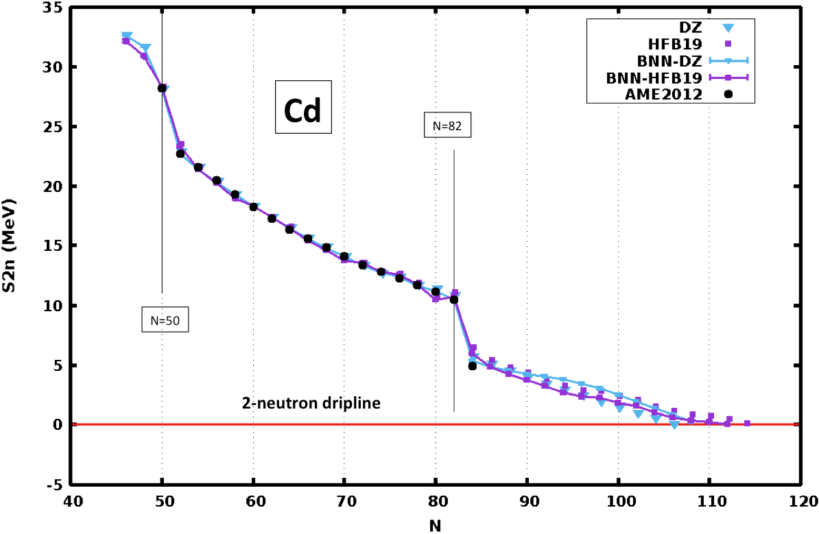
Figure 6: Two-neutron separation energies for all even-even cadmium isotopes from ⁹⁴Cd to ¹⁶⁴Cd, as predicted by the mic-mac model of Duflo and Zuker Duflo and Zuker (1995) and the microscopic HFB19 model Goriely et al. (2010). Predictions are displayed without error bars for the bare models and with error bars after the BNN refinement. Experimental data are from Ref. Wang et al. (2012a).

We conclude this section by displaying in Fig. 6 two-neutron separation energies for all even-even isotopes in cadmium: from ⁹⁴Cd to ¹⁶⁴Cd. Clearly discernible in the figure is the characteristic “jumps” at magic numbers 50 and 82. The figure also encapsulates the inherent risk in extrapolating theoretical models far away from regions where experimental information is available. Whereas the models agree where data is available (from $50\!\leq\!N\!\leq\!82$), the model-discrepancy grows gradually with increasing neutron numbers. And while the BNN refinement is successful in mitigating the problem up to $N\!\lesssim\!90$ (see Fig. 5c), the BNN predictions for $S_{2n}$ can differ by $\sim\!1$ MeV far away from stability. This situation is reminiscent of the one addressed in Ref. Erler et al. (2012) for $S_{2n}$ in the case of the even-even erbium ($Z\!=\!68$) isotopes. It was found there that the discrepancy between various model predictions steadily grows with neutron excess as a result of the poorly known isovector effective interaction. Indeed, models that are successful in reproducing the experimentally determined two-neutron separation energy, differ in their predictions of the location of the neutron drip line by as many as eight neutrons. Fortunately, next-generation rare-isotope facilities will produce hundreds of new exotic nuclei very far away from stability that will help constrain the isovector sector. Yet a most pressing challenge is to identify the “few” critical nuclei that will best inform nuclear theory. We are confident that the BNN formalism will successfully meet this challenge.

V Conclusions

The quest for the nuclear driplines is at the heart of one of the central themes animating nuclear physics today: what are the limits of nuclear existence? As a fundamental nuclear-structure problem, the driplines define the most extreme combinations of protons and neutrons that can remain bound by the strong nuclear force. Drip-line nuclei are weakly bound, finite, strongly correlated quantum systems where the virtual coupling to the continuum is critical. Besides being of intrinsic interest in nuclear structure, nuclei far away from stability also play a predominant role in astrophysics; for example, in stellar nucleosynthesis and in neutron stars. However, the enormous theoretical challenges faced in describing exotic nuclei are compounded by the lack of experimental guidance. For example, theoretical predictions seem to suggest that ¹¹⁸Kr is the drip-line nucleus separating the inner and outer crust of neutron stars. Yet ¹¹⁸Kr is 21 neutrons away from the last well-measured isotope. Thus, having to resort to extrapolations seems unavoidable.

Undoubtedly, large extrapolations pose a considerable risk. In an effort to mitigate such risk we proposed a novel approach based on the construction of an artificial neural network. Moreover, given that the neural-network parameters are determined through Bayesian inference, our results are accompanied by statistical uncertainties. The proposed approach adopts a highly successful mass model that is then refined through the construction of an artificial neural network. Briefly, the implementation of the BNN refinement proceeds by dividing the existing experimental database of nuclear masses into a learning and a validation set, with the members of each set selected at random. One then uses the learning set to train the artificial neural network by focusing on the mass residuals, i.e., on the difference between the experimentally measured and predicted mass. The validation set is then used to test the robustness and reliability of the refined model. If a significant improvement relative to the bare model is observed, then the training is repeated but now using the entire experimental database. Although we developed most of these ideas using the relatively simple, yet highly accurate, 10-parameter Duflo-Zuker model, our ultimate goal was to publish refined mass tables for two existing mass models, one microscopic and the other one of the mic-mac type. For the latter we used the 28-parameter Duflo-Zuker model while for the former HFB19.

These are some of the most salient conclusions of our work. First, despite the intrinsic high-quality of both mass models, the BNN refinement lead to a significant improvement: $\sigma_{\rm rms}\!=\!(0.503\rightarrow 0.286)$ MeV and $\sigma_{\rm rms}\!=\!(0.559\rightarrow 0.358)$ MeV for DZ and HFB19, respectively. Second, although theoretical mass models agree in regions where masses are known but differ widely in regions where they are not, we found a systematic and significant reduction in the model spread after implementing the BNN refinement. Third, given the Bayesian character of the approach, all BNN refined predictions are now accompanied by theoretical uncertainties. Finally, we provided as supplemental material mass tables, as well as tables for other derived quantities such as separation energies, for the two BNN refined models considered in this work. We trust that these refined mass tables will be helpful for future astrophysical applications.