Natural extensions of unimodal maps: virtual sphere homeomorphisms and prime ends of basin boundaries.

Abstract.

Let $\{f_{t}\colon I\to I\}$ be a family of unimodal maps with topological entropies $h(f_{t})>\frac{1}{2}\log 2$, and ${\widehat{f}}_{t}\colon{\widehat{I}}_{t}\to{\widehat{I}}_{t}$ be their natural extensions, where ${\widehat{I}}_{t}=\varprojlim(I,f_{t})$. Subject to some regularity conditions, which are satisfied by tent maps and quadratic maps, we give a complete description of the prime ends of the Barge-Martin embeddings of ${\widehat{I}}_{t}$ into the sphere. We also construct a family $\{\chi_{t}\colon S^{2}\to S^{2}\}$ of sphere homeomorphisms with the property that each $\chi_{t}$ is a factor of ${\widehat{f}}_{t}$, by a semi-conjugacy for which all fibers except one contain at most three points, and for which the exceptional fiber carries no topological entropy: that is, unimodal natural extensions are virtually sphere homeomorphisms. In the case where $\{f_{t}\}$ is the tent family, we show that $\chi_{t}$ is a generalized pseudo-Anosov map for the dense set of parameters for which $f_{t}$ is post-critically finite, so that $\{\chi_{t}\}$ is the completion of the unimodal generalized pseudo-Anosov family introduced in [21].

1. Introduction

1.1. Overview

The study of continua and their rich topological structures goes back to the first half of the $20^{\text{th}}$ century, and played a central rôle in the early development of topology. Embeddings of continua in surfaces have also been an important ingredient in dynamical systems theory: early examples include Birkhoff’s remarkable curves [11, 29] and the Cartwright-Littlewood Theorem [19]. Williams [40, 41] was the first to notice, in the late 1960s, that continua defined by inverse limits are a useful tool in the study of dynamical systems: specially relevant here is his discovery that a particular class of planar continua, the inverse limits of expanding maps on graphs, describe planar, one-dimensional hyperbolic attractors. In the early 1990s — inspired in part by the importance of the Hénon family as a paradigm for the larger family of non-hyperbolic attractors — Barge and Martin [10, 14] gave a method to embed a wide class of inverse limits as attractors of planar homeomorphisms. The inverse limits of unimodal maps of the interval such as those from the quadratic and tent families are of particular importance for the Hénon family. These inverse limits are the chief objects of study here. A simple example is shown in Figure 1 for expository purposes: it will be used as a point of reference throughout the introduction.

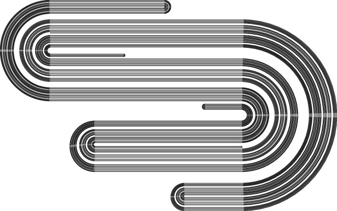
Figure 1. An approximation of the inverse limit of a tent map with kneading sequence $(1001110)^{\infty}$, which is of rational interior type with height $1/3$ (see below).

The prime ends of the complementary domains form an essential part of the analysis of planar continua: in dynamical systems, they have been used in the description of basin boundaries [2, 33] and, in the wider context of holomorphic dynamics, prime ends of the complements of Julia sets [12, 20, 28, 38] have also been studied. In this paper we give a complete description of the prime ends of the complementary domains of the Barge-Martin embeddings of the inverse limits of families of unimodal maps. We believe that this constitutes the first complete analysis in the literature of the nature of the embeddings of a continuously varying family of planar attractors. (In subsequent work using more symbolic techniques, Anušić and Činč [5] reproduce most of the results here about the prime ends of Barge-Martin embeddings in the specific case of tent map inverse limits, and enhance our results in this case with additional topological information concerning folding points and endpoints.)

The topology of unimodal inverse limits is exquisitely complicated. For the tent family $\{f_{t}\}$, results of Bruin and of Raines [18, 37] imply that, when the parameter $t$ is such that the critical orbit of $f_{t}$ is dense (a full measure, dense $G_{\delta}$ set of parameters), the inverse limit ${\widehat{I}}_{t}$ is nowhere locally the product of a Cantor set and an interval, and is therefore much more complicated than the example of Figure 1. A striking statement of self-similarity is given by Barge, Brucks and Diamond [7], who show that there is a dense $G_{\delta}$ set of parameters $t$ for which every open subset of ${\widehat{I}}_{t}$ contains a homeomorphic copy of ${\widehat{I}}_{s}$ for every $s\in[\sqrt{2},2]$. Moreover, the Ingram conjecture posits that the inverse limits ${\widehat{I}}_{t}$ are pairwise non-homeomorphic. This has been proved for non-core tent maps by Barge, Bruin, and Štimac [8], while for core tent maps there are known to be uncountably many homeomorphism classes (see for example [4, 25]).

In the second part of the paper, we show that all of these inverse limit spaces are virtually spheres: there are quotients $p_{t}\colon{\widehat{I}}_{t}\to S^{2}$ which respect the natural extensions ${\widehat{f}}_{t}\colon{\widehat{I}}_{t}\to{\widehat{I}}_{t}$, and have the property that, with the exception of at most one $x\in S^{2}$, the fiber $p_{t}^{-1}(x)$ contains at most three points: moreover, the exceptional fiber carries no topological entropy. There is therefore a family $\{\chi_{t}\}$ of sphere homeomorphisms — which is shown to vary continuously — such that

$$\begin{CD}S^{2}@>{\chi_{t}}>{}>S^{2}\\ @A{p_{t}}A{}A@A{}A{p_{t}}A\\ {\widehat{I}}_{t}@>{{\widehat{f}}_{t}}>{}>{\widehat{I}}_{t}\\ @V{\pi_{0}}V{}V@V{}V{\pi_{0}}V\\ I@>{f_{t}}>{}>I\\ \end{CD}$$

commutes (here $\pi_{0}\colon{\widehat{I}}_{t}\to I$ is projection onto the first coordinate). In view of the mildness of the semi-conjugacies $p_{t}$, this suggests that the sphere is a natural space on which to study invertible analogs of unimodal maps.

The sphere homeomorphisms $\chi_{t}$ are best seen as generalizations of Thurston’s pseudo-Anosov maps [39]. A pseudo-Anosov homeomorphism $\phi$ of a surface has a transverse pair of invariant singular foliations, one stable and one unstable, which fill the surface. Collapsing the stable foliation yields a graph, the train track, which carries an expanding map. Following Williams, the inverse limit of the train track map yields a homeomorphism $\Phi$ with a one-dimensional hyperbolic attractor. This homeomorphism can alternatively be obtained by “DA-ing” the prongs of the pseudo-Anosov foliations, i.e., splitting open the leaves ending at the pronged singularities. The original pseudo-Anosov map $\phi$ can be reconstructed from $\Phi$ by “collapsing” stable sets in the complement of the attractor.

The process used to construct the sphere homeomorphisms $\chi_{t}$ formalizes and generalizes this last collapse: we start with the Barge-Martin embedding of the inverse limit of a unimodal map $f_{t}$ as an attactor, and collapse strongly stable sets (see Definition 5.1) to obtain $\chi_{t}$. In Figure 1 the semi-circular arcs represent identifications, and are not part of the inverse limit, which consists only of the horizontal arcs. With this in mind, the quotient can be seen — although not quite accurately — as being obtained by collapsing, in each vertical line, the closure of the segments in the complement of the attractor, and then sewing up the outside in a dynamically coherent way. Because the inverse limit of a general unimodal map can be much more complicated than that of a train track map, the dynamics and invariant geometric structures of $\chi_{t}$ are correspondingly more complicated. In particular, the invariant stable and unstable “foliations” are only defined in a measurable sense.

In the case where $\{f_{t}\}$ is the tent family, the corresponding family $\{\chi_{t}\}$ is a completion of the family of generalized pseudo-Anosov maps which was constructed in [21] for post-critically finite tent maps. (A generalized pseudo-Anosov is defined similarly to a pseudo-Anosov, except that its invariant foliations can have infinitely many singularities, provided they accumulate on only finitely many points: see Definition 5.27.) The earlier construction was explicit, and made essential use of the existence of finite Markov partitions. The constructions of this paper show not only how generalized pseudo-Anosovs arise directly from inverse limits and natural extensions — with the leaves of the unstable foliation of $\chi_{t}$ coming from the path components of the inverse limit of $f_{t}$ — but also how they live within the richer class of homeomorphisms which arise in the post-critically infinite case. These measurable pseudo-Anosov homeomorphisms, whose invariant foliations are only defined on a full measure subset of the sphere, are the subject of articles in preparation.

For the countable set of NBT parameters introduced in [26], the map $\chi_{t}$ is an actual pseudo-Anosov homeomorphism. Thus the analysis of the family $\chi_{t}$ also contributes to the question of the completion in the $C^{0}$-topology of the set of all pseudo-Anosov homeomorphisms on a given surface.

1.2. Background

We now proceed to a brief overview of some background theory in dynamics and topology, which will enable us to give more precise statements of our main results in Sections 1.3 and 1.4 below.

1.2.1. Unimodal maps

The study of unimodal maps of the interval, one of the simplest classes of dynamical systems which exhibit complicated behavior, drove the development of the theory of topological dynamical systems in the 1970s and beyond. A continuous map $f\colon[a,b]\to[a,b]$ is said to be (non-core) unimodal if

1. $f(a)=f(b)=a$, and

2. there is a turning point $c\in(a,b)$ such that $f$ is strictly increasing on $[a,c]$ and strictly decreasing on $[c,b]$. Moreover $f(x)>x$ for $x\in(a,c]$.

The qualification non-core is important here: we will shortly replace condition (a) with an alternative version which corresponds to restricting the domain to an invariant sub-interval (the core) in which all of the non-trivial dynamics is contained.

Prototypical examples of families of unimodal maps are the quadratic (also known as logistic) and tent families $f_{t}\colon[0,1]\to[0,1]$ defined respectively by

$$f_{t}(x)=tx(1-x)\quad(0<t\leq 4)\qquad\text{ and }\qquad f_{t}(x)=t\min\{x,1-x\}\quad(0<t\leq 2).$$

The tent family is of particular theoretical importance, because any unimodal map $f\colon[a,b]\to[a,b]$ with positive topological entropy $h(f)$ (a numerical measure of the asymptotic rate at which the orbits of nearby points diverge from each other [1]) is semi-conjugate to the tent map with slope $t=\exp(h(f))$ [31, 36]. That is, there is an increasing surjection $p\colon[a,b]\to[0,1]$ such that

$$\begin{CD}[a,b]@>{f}>{}>[a,b]\\ @V{p}V{}V@V{}V{p}V\\ [0,1]@>{f_{t}}>{}>[0,1]\\ \end{CD}$$

commutes, so that the dynamics of $f$ and of the tent map $f_{t}$ agree once certain intervals in the domain of $f$ — the nontrivial point preimages $p^{-1}(x)$ — have been collapsed. The semi-conjugacy $p$ can be described explicitly, by means either of a formula, or of a dynamical description of exactly which intervals in the domain of $f$ are collapsed.

Kneading theory is a key tool in the analysis of the dynamics of unimodal maps. Points $x\in[a,b]$ are described by their itineraries $\iota(x)\in\{0,1\}^{\mathbb{N}}$, sequences of $0$s and $1$s which encode, for each successive point on the orbit of $x$, whether it is on the left (‘$0$’) or the right (‘$1$’) of the turning point $c$. (The details of how to encode $c$ itself are largely unimportant in this paper, and are left for Section 2.1.) The itinerary of $f(c)$, the largest point in the range of $f$, is of particular importance, and is called the kneading sequence $\kappa(f)$ of $f$. The dynamics of $f$ is largely determined by its kneading sequence — in particular, $\kappa(f)$ determines the topological entropy $h(f)$, and hence the particular tent map to which $f$ is semi-conjugate.

The unimodal order (or parity-lexicographic order) $\preceq$ on $\{0,1\}^{\mathbb{N}}$ is defined (see Definition 2.3) to reflect the ordering of the interval: if $x<y$, then $\iota(x)\preceq\iota(y)$. However, it takes on more meaning when interpreted as an order on the space of unimodal maps: if $\kappa(f)\preceq\kappa(g)$, then the dynamics of $g$ is at least as complicated as the dynamics of $f$. In particular, $\kappa(f_{t})$ is an increasing function of $t$ if $f_{t}$ is either the quadratic or the tent family.

The core of a unimodal map $f\colon[a,b]\to[a,b]$ is the interval $J=[f^{2}(c),f(c)]$. It satisfies $f(J)=J$: moreover, the orbit of every $x\in(a,b)$ falls into $J$, so that all of the non-trivial recurrent dynamics of $f$ is contained in the core. For this reason, it is sensible — particularly when considering inverse limits — to restrict the domain of a unimodal map to its core. This corresponds to replacing the condition that $f(a)=f(b)=a$ with the condition that $f(c)=b$ and $f(b)=a$.

In this paper we will be exclusively concerned with core unimodal maps, and Definition 2.1 reflects this. We impose some additional conditions on our unimodal maps $f$, which are stated in Convention 2.8 below. These conditions are of two types:

1. Regularity conditions, expressed in a way which allows them to encompass both the quadratic family and the tent family. These conditions appear technical, but are standard in the theory of unimodal maps.

2. The additional condition that $f$ has topological entropy $h(f)>\frac{1}{2}\log 2$. This is an indecomposability condition: it is equivalent to the non-existence of a pair of subintervals $J_{1}$, $J_{2}$, disjoint except perhaps at their endpoints, with $f(J_{1})\subset J_{2}$ and $f(J_{2})\subset J_{1}$.

Readers without a background in one-dimensional dynamics can substitute “a unimodal map satisfying the conditions of Convention 2.8” with “a map from the quadratic or tent family with sufficiently large parameter”, without substantial loss.

1.2.2. Inverse limits

Let $X$ be a compact metric space with metric $d$, and let $f\colon X\to X$ be continuous and surjective. The inverse limit of $f\colon X\to X$ is the space of “backwards orbits” of $f$:

$${\widehat{X}}:=\varprojlim(X,f)=\{{\mathbf{x}}\in X^{\mathbb{N}}\,:\,f(x_{i+1})=x_{i}\text{ for all }i\in{\mathbb{N}}\}.$$

We endow ${\widehat{X}}$ with a standard metric, also denoted $d$, which induces its natural topology as a subspace of the product $X^{\mathbb{N}}$:

$$d({\mathbf{x}},{\mathbf{y}})=\sum_{i=0}^{\infty}\frac{d(x_{i},y_{i})}{2^{i}}.$$

Elements of ${\widehat{X}}$ are denoted with angle brackets, ${\mathbf{x}}=\left<x_{0},x_{1},x_{2},\ldots\right>$ and referred to as threads.

The natural extension of $f\colon X\to X$ is the homeomorphism ${\widehat{f}}\colon{\widehat{X}}\to{\widehat{X}}$ defined by

$${\widehat{f}}(\left<x_{0},x_{1},x_{2},\ldots\right>)=\left<f(x_{0}),x_{0},x_{1},x_{2},\ldots\right>.$$

The projection $\pi_{0}\colon{\widehat{X}}\to X$ is defined by $\pi_{0}({\mathbf{x}})=x_{0}$. Clearly $\pi_{0}\circ{\widehat{f}}=f\circ\pi_{0}$, so that $\pi_{0}$ semi-conjugates ${\widehat{f}}$ to $f$. It is straightforward to show that if $g\colon Y\to Y$ is an invertible dynamical system and $p\colon Y\to X$ semi-conjugates $g$ to $f$, then $p$ factors through $\pi_{0}$: therefore the natural extension is the simplest invertible system which has $f$ as a factor.

1.2.3. The Barge-Martin construction

The Barge-Martin construction [10] provides a mechanism for embedding the inverse limit ${\widehat{X}}$ of a dynamical system $f\colon X\to X$ as a global attractor of a self-homeomorphism of a manifold, on which the homeomorphism restricts to the natural extension of $f$. We now give a brief outline of the construction in the case of interest here, where $f\colon I\to I$ is a unimodal map whose inverse limit is embedded as an attractor of a sphere homeomorphism. Further details can be found in Section 2.2.

Let $T$ be a topological sphere, $D\subset T$ be a closed disk containing a copy of $I$ in its interior, and $\partial$ be a point of $T\setminus D$. Construct a smash $\Upsilon\colon T\to T$, a near-homeomorphism (i.e. a uniform limit of homeomorphisms) which

• collapses $D$ onto $I$, in such a way that the preimage of each point of $I$ is an arc in $D$;

• fixes $\partial$; and

• pushes points of $T\setminus(D\cup\{\partial\})$ “inwards” towards $I$.

Let $\overline{f}\colon T\to T$ be an unwrapping of $f$: a near-homeomorphism which

• sends $I$ into $D$ in such a way that $\Upsilon\circ\overline{f}|_{I}=f$; and

• doesn’t push any points of $T\setminus\{\partial\}$ too far “outwards”.

Now consider the near-homeomorphism $H=\Upsilon\circ\overline{f}\colon T\to T$. By construction we have $H|_{I}=f$, so that the inverse limit ${\widehat{T}}=\varprojlim(T,H)$ contains an embedded copy of ${\widehat{I}}$, namely $\{{\mathbf{x}}\in{\widehat{T}}\,:\,x_{i}\in I\text{ for all }i\}$, on which the action of the natural extension ${\widehat{H}}$ restricts to ${\widehat{f}}$. Because the smash pushes points of $T$ other than $\partial$ towards $I$ more strongly than the unwrapping pushes them away, every point of ${\widehat{T}}$ other than $\left<\partial,\partial,\partial,\dots\right>$ is attracted to the copy of ${\widehat{I}}$ under iteration of ${\widehat{H}}$.

The key observation is that the inverse limit ${\widehat{T}}$ is itself a topological sphere, as a consequence of the following theorem due to Morton Brown:

Theorem (Brown [16]).

Let $X$ be a compact metric space, and $f\colon X\to X$ be a near-homeomorphism. Then $\varprojlim(X,f)$ is homeomorphic to $X$.

The constructions in this paper depend crucially on the details of the smash $\Upsilon$ (see Section 2.2), and on the careful definition of a particular choice of unwrapping $\overline{f}$, which is described in Section 3.

1.2.4. Prime ends

We will describe the Barge-Martin embedding of the inverse limit ${\widehat{I}}$ of a unimodal map $f$ in the topological sphere ${\widehat{T}}$ by means of Carathéodory’s theory of prime ends. Here we review some basic definitions in order to allow for precise statements of our main results. We note that while the theory of prime ends can be profitably approached from the viewpoint of conformal mappings, the spaces which we will be dealing with have no natural complex structure, and so we take a purely topological approach. The reader seeking a more comprehensive introduction from this point of view could consult, for example, Mather’s paper [30].

Let $T$ be a topological $2$-sphere, and $X$ be a non-empty, compact, connected, non-separating proper subset of $T$, so that the complement $U:=T\setminus X$ is a topological open disk. (For most of our applications, $T$ will be the sphere ${\widehat{T}}$ of the Barge-Martin embedding, and $X$ will be the embedded copy of ${\widehat{I}}$.) Fix a point $\partial\in U$.

A crosscut (in $(T,X)$) is an arc $\xi$ in $T$ which is disjoint from $\partial$ and intersects $X$ exactly at the endpoints of $\xi$. Such a crosscut separates the open disk $U$ into two components, and we write $U(\xi)$ for the component which doesn’t contain $\partial$. If $\xi_{1}$ and $\xi_{2}$ are crosscuts, then we write $\xi_{2}<\xi_{1}$ to mean that $U(\xi_{2})\subset U(\xi_{1})$. A chain is a sequence $(\xi_{k})$ of disjoint crosscuts with $\xi_{k+1}<\xi_{k}$ for each $k$ and $\operatorname{diam}(\xi_{k})\to 0$ as $k\to\infty$. Two chains $(\xi_{k})$ and $(\xi_{k}^{\prime})$ are equivalent if for each $k$ there is some $K$ with $\xi_{K}<\xi_{k}^{\prime}$ and $\xi_{K}^{\prime}<\xi_{k}$.

A prime end (of $(T,X)$) is an equivalence class of chains of crosscuts in $(T,X)$.

Let ${\mathcal{P}}$ be a prime end of $(T,X)$. The principal set $\Pi({\mathcal{P}})$ of ${\mathcal{P}}$ is the set of points $x\in X$ for which there is some chain $(\xi_{k})$ representing ${\mathcal{P}}$ with $d(\xi_{k},x)\to 0$ as $k\to\infty$. The impression ${\mathcal{I}}({\mathcal{P}})$ of ${\mathcal{P}}$ is defined by

$${\mathcal{I}}({\mathcal{P}})=\bigcap_{k\geq 0}\overline{U(\xi_{k})},$$

where $(\xi_{k})$ is a chain representing ${\mathcal{P}}$ (the definition is clearly independent of the choice of chain). We therefore have

$$\emptyset\not=\Pi({\mathcal{P}})\subseteq{\mathcal{I}}({\mathcal{P}})\subseteq X.$$

According to Carathéodory’s classification, a prime end ${\mathcal{P}}$ is of the

First kind:

if $\Pi({\mathcal{P}})={\mathcal{I}}({\mathcal{P}})$ is a point;

Second kind:

if $\Pi({\mathcal{P}})$ is a point and is strictly contained in ${\mathcal{I}}({\mathcal{P}})$;

Third kind:

if $\Pi({\mathcal{P}})={\mathcal{I}}({\mathcal{P}})$ is not a point; and

Fourth kind:

if $\Pi({\mathcal{P}})$ is not a point and is strictly contained in ${\mathcal{I}}({\mathcal{P}})$.

The language of rays is helpful in developing an intuitive understanding of principal sets and impressions. A ray in $(T,X)$ is a continuous injection $\sigma\colon[0,\infty)\to U$ with $d(\sigma(s),X)\to 0$ as $s\to\infty$. The remainder $\operatorname{Rem}(\sigma)$ of $\sigma$ is the set $\overline{\sigma([0,\infty))}\cap X$. We say that $\sigma$ lands (and that its landing point is $x\in X$) if $\operatorname{Rem}(\sigma)=\{x\}$. A point $x\in X$ is accessible if it is the landing point of some ray.

Let ${\mathcal{P}}$ be a prime end defined by a chain $(\xi_{k})$. A ray $\sigma$ converges to ${\mathcal{P}}$ if for every $k$ there is some $t$ such that $\sigma([t,\infty))\subset U(\xi_{k})$: in particular, this means that the image of $\sigma$ intersects $\xi_{k}$ for all sufficiently large $k$.

It can be shown that if $\sigma$ converges to ${\mathcal{P}}$, then $\Pi({\mathcal{P}})\subseteq\operatorname{Rem}(\sigma)\subseteq{\mathcal{I}}({\mathcal{P}})$: in particular, if $\sigma$ lands at an accessible point $x\in X$, then $\Pi({\mathcal{P}})=\{x\}$. Moreover, there are rays $\sigma,\sigma^{\prime}$ converging to ${\mathcal{P}}$ with $\operatorname{Rem}(\sigma)=\Pi({\mathcal{P}})$ and $\operatorname{Rem}(\sigma^{\prime})={\mathcal{I}}({\mathcal{P}})$. Thus the principal set and impression of ${\mathcal{P}}$ can be seen, respectively, as the remainders of the “tightest” and “loosest” rays converging to ${\mathcal{P}}$.

Let ${\mathbb{P}}$ denote the set of prime ends of $(T,X)$. There is a natural topology on ${\mathbb{P}}$, with respect to which it is a topological circle: a basis for this topology is given by the subsets ${\mathcal{B}}(\xi)$ of ${\mathbb{P}}$, defined for each crosscut $\xi$ to consist of all of the prime ends defined by chains $(\xi_{k})$ with $\xi_{k}<\xi$ for some $k$. (In fact, this is the subspace topology of a natural topology on ${\mathbb{P}}\cup U$, with respect to which this space is a compact disk; and the definition above of a ray converging to a prime end is the normal notion of convergence with respect to this topology.)

A homeomorphism $H\colon(T,X)\to(T,X)$ (such as the natural extension ${\widehat{H}}\colon({\widehat{T}},{\widehat{I}})\to({\widehat{T}},{\widehat{I}})$ of the Barge-Martin construction) induces a self-homeomorphism of the circle ${\mathbb{P}}$ which sends the prime end represented by a chain $(\xi_{k})$ to the prime end represented by $(H(\xi_{k}))$. The prime end rotation number of $H\colon(T,X)\to(T,X)$ is the Poincaré rotation number of this circle homeomorphism.

1.2.5. Height

Let $\{f_{t}\}$ be a family of core unimodal maps of an interval $I$ satisfying the assumptions of Convention 2.8, such as the quadratic or tent family with topological entropy greater than $\frac{1}{2}\log 2$. The Barge-Martin construction yields (abstract) sphere homeomorphisms ${\widehat{H}}_{t}\colon{\widehat{T}}_{t}\to{\widehat{T}}_{t}$, having attractors $\Lambda_{t}$ which are homeomorphic to the inverse limits ${\widehat{I}}_{t}:=\varprojlim(I,f_{t})$, and restricted to which the homeomorphisms ${\widehat{H}}_{t}$ are conjugate to the natural extensions of $f_{t}$.

In the first part of the paper we study the prime ends of $({\widehat{T}}_{t},\Lambda_{t})$. In the second part we construct sphere homeomorphisms $\chi_{t}$ by collapsing a system of subsets of ${\widehat{T}}_{t}$, which are permuted by ${\widehat{H}}_{t}$, such that

• each subset intersects $\Lambda_{t}$ in at least one point; and

• each subset except at most one intersects $\Lambda_{t}$ in only finitely many points.

The former of these properties ensures that there is a semiconjugacy $p_{t}$ from ${\widehat{f}}_{t}$ to $\chi_{t}$, and the latter that all but at most one of the fibers of $p_{t}$ is finite.

Both the structure of the prime ends and the construction of the semiconjugacy (including the nature of its exceptional fiber) are heavily dependent on the parameter $t$, or, to be more precise, on the height $q(f_{t})$ of $f_{t}$ [26] (Section 2.4). Dynamically, the height is the prime end rotation number of ${\widehat{H}}_{t}\colon({\widehat{T}}_{t},\Lambda_{t})\to({\widehat{T}}_{t},\Lambda_{t})$. It is an element of $[0,1/2]$, dependent only on the kneading sequence $\kappa(f_{t})$ of $f_{t}$, which decreases as $\kappa(f_{t})$ increases in the unimodal order, with each irrational height being realized by a single kneading sequence, and each rational height being realized on a closed height interval of kneading sequences. See Figure 2, which shows how height varies in the quadratic family. The assumption that $h(f_{t})>\frac{1}{2}\log 2$ is, in fact, equivalent to $q(f_{t})<1/2$ (Lemma 2.22).

It follows that every unimodal map $f$ is of one of three types:

Irrational:

when $q(f)$ is irrational;

Rational interior:

when $\kappa(f)$ is in the interior of the interval of kneading sequences of some rational height $m/n$; or

Rational endpoint:

when $\kappa(f)$ is an endpoint of the interval of kneading sequences of some rational height $m/n$.

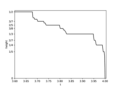
Figure 2. Height $q(f_{t})$ for the quadratic family $f_{t}(x)=tx(1-x)$.

1.3. Prime ends of Barge-Martin attractors

The results of Theorems 4.46, 4.64, and 4.66, together with Remarks 4.47, 4.65, and 4.71 are summarized in the following statement, where we refer to a prime end of the first kind (whose impression is a point) as trivial. As discussed in Section 1.2.1, the hypothesis of this theorem is satisfied by the tent and quadratic families with topological entropy greater than $\frac{1}{2}\log 2$.

Theorem.

Let $\{f_{t}\}$ be a family of unimodal maps satisfying the assumptions of Convention 2.8. Then the prime ends of the Barge-Martin attractor of $f_{t}$ in the sphere satisfy the following.

1. If $f_{t}$ is of irrational type, then the set of non-trivial prime ends is a Cantor set. These non-trivial prime ends are of the second kind, with impression the whole attractor.

2. If $f_{t}$ is of rational endpoint type with height $m/n$, then there are exactly $n$ non-trivial prime ends, which are of the second kind, with impression the whole attractor.

3. If $f_{t}$ is of rational interior type with height $m/n$, then there are exactly $n$ non-trivial prime ends, whose impressions are the whole attractor. These are of the third kind (the principal set is also the whole attractor), unless $f_{t}$ belongs to a particular renormalization window at the start of the $m/n$ height interval, in which case they are of the fourth kind.

4. If $f_{t}$ is of rational type with height $m/n$ then the attractor has $n$ components of accessible points; while if $f_{t}$ is of irrational type then the attractor has infinitely many components of accessible points (countably many intervals and uncountably many points).

For the example of Figure 1, which depicts the inverse limit of a tent map $f_{t}$ of rational interior type with height $1/3$, there are three infinite “tunnels”, corresponding to the three non-trivial prime ends, which become stepwise narrower and narrower as they probe deeper and deeper into the inverse limit. The natural extension stretches by a factor $t$ in the horizontal direction, contracts by a factor $1/t$ in the vertical direction, and bends the image around as dictated by $f_{t}$ (see for example Figure 8): thus the three tunnels are permuted by the action, and so are the three non-trivial prime ends, with rotation number $1/3$ equal to the height. By comparison, Figure 3 depicts an example of rational interior type with height $2/7$, where there are seven infinite tunnels which are permuted with rotation number $2/7$; and Figure 4 depicts an example of rational endpoint type with height $1/3$: here there are infinitely many tunnels into the inverse limit, but all of them are finite.

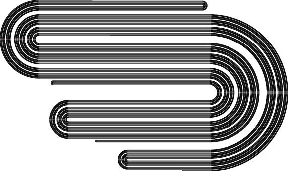
Figure 3. An example of rational interior type with height $2/7$.

Figure 4. An example of rational endpoint type with height $1/3$.

We now give an informal overview of the main steps in the proof of this theorem, dropping the dependence on $t$ for the sake of clarity. In Section 3.2 we construct an explicit unwrapping of $f$ to be used as the starting point of the Barge-Martin construction, based on the outside map $B\colon S\to S$ of $f$ (Section 3.1), a monotone circle map which describes the “thickened” action of $f$ as seen from a circle around $I$, whose rotation number is equal to the height $q(f)$ of $f$. The explicit nature of the unwrapping provides a description of the elements of ${\widehat{T}}\setminus\Lambda$ which makes it possible to construct explicit chains of cross cuts to determine the prime ends (see for example Figure 11). The key part of this process is the definition of a homeomorphism $\Psi\colon{\widehat{S}}\times[0,\infty)/({\widehat{S}}\times\{0\})\to{\widehat{T}}\setminus\Lambda$ (Section 4.1), where ${\widehat{S}}$ is the inverse limit of the outside map, which provides a coordinate system on ${\widehat{T}}\setminus\Lambda$ in which these crosscuts can be described in a straightforward way. Because the space ${\widehat{S}}$ depends on the dynamics of the outside map, which is strongly dependent on its rotation number (Theorem 4.33), the structure of the prime ends themselves is strongly dependent on the height.

1.4. Semi-conjugacy to a family of sphere homeomorphisms

The results of Theorems 5.19 and 5.31 are summarized in the following statement.

Theorem.

Let $\{f_{t}\}$ be a family of unimodal maps satisfying the assumptions of Convention 2.8. Then there is a continuously varying family $\{\chi_{t}\colon S^{2}\to S^{2}\}$ of sphere homeomorphisms such that each natural extension ${\widehat{f}}_{t}\colon{\widehat{I}}_{t}\to{\widehat{I}}_{t}$ is semi-conjugate to $\chi_{t}$, by a semi-conjugacy all but one of whose fibers contains three or fewer points, and only countably many of whose fibers contain three points.

If $\{f_{t}\}$ is the tent family, then for each parameter $t$ for which $f_{t}$ is post-critically finite, the sphere homeomorphism $\chi_{t}$ is a generalized pseudo-Anosov map.

The exceptional fiber depends on the type of the unimodal map $f_{t}$. In the tent family case, where different parameters give rise to different kneading sequences, there is a particularly clean description of these fibers:

• if $f_{t}$ is of irrational type, then the exceptional fiber is a Cantor set;

• if $f_{t}$ is of rational interior type with height $m/n$, then the exceptional fiber is finite with cardinality $n$; and

• if $f_{t}$ is of rational endpoint type with height $m/n$, then the exceptional fiber is countable with $n$ accumulation points.

In particular, the set of parameters for which the exceptional fiber is infinite is a Cantor set. In the general case the description is more complicated in an initial subinterval of each height interval, and the exceptional fibre may contain arcs for parameters in these subintervals (see Remark 5.17). In all cases no fiber of the semi-conjugacy carries entropy, so no entropy is lost in the quotient.

For each parameter $t$, the sphere homeomorphism $\chi_{t}$ is constructed from the Barge-Martin homeomorphism ${\widehat{H}}_{t}\colon{\widehat{T}}_{t}\to{\widehat{T}}_{t}$ by collapsing the elements of an ${\widehat{H}}_{t}$-invariant decomposition ${\mathcal{G}}_{t}$ of ${\widehat{T}}_{t}$. The decompositions are dynamically defined, their elements being determined by the strongly stable components of ${\widehat{H}}_{t}$. The homeomorphism $\Psi_{t}\colon{\widehat{S}}_{t}\times[0,\infty)/({\widehat{S}}_{t}\times\{0\})\to{\widehat{T}}_{t}\setminus\Lambda_{t}$ enables these components to be described explicitly, with their configuration determined by the type of the unimodal map $f_{t}$ (see Figures 14, 15, 16, and 17). From these descriptions, it can be shown that each ${\mathcal{G}}_{t}$ is a non-separating, monotone, upper semicontinuous decomposition, whose elements all intersect $\Lambda_{t}$, with at most one element intersecting $\Lambda_{t}$ in more than three points. It follows from Moore’s theorem [32] that the quotient space ${\widehat{T}}_{t}/{\mathcal{G}}_{t}$ is itself a sphere, and the quotient homeomorphism ${\widehat{H}}_{t}/{\mathcal{G}}_{t}$ has the required properties.

Since these quotient homeomorphisms are all defined on different abstract spheres, some further work is needed to show that they can be conjugated to a continuous family of homeomorphisms of a standard sphere. The key result here is a theorem of Dyer and Hamstrom [23], Theorem 5.22, which requires, roughly speaking, that if we take the three-dimensional space obtained by piecing together the spheres ${\widehat{T}}_{t}$, then the decomposition of this space obtained from the ${\mathcal{G}}_{t}$ is itself upper semicontinuous. That this is the case follows once more from the explicit descriptions of the ${\mathcal{G}}_{t}$ (see Section 5.4).

That the dynamics of the sphere homeomorphisms $\chi_{t}$ closely mimic those of the unimodal maps $f_{t}$ is expressed by the following straightforward result (see Theorem 5.32).

Theorem.

Let $f$ be a unimodal map satisfying the conditions of Convention 2.8, and $\chi\colon S^{2}\to S^{2}$ be the corresponding semi-conjugate sphere homeomorphism. Then

1. if $f$ is topologically transitive then so is $\chi$;

2. if $f$ has dense periodic points, then so does $\chi$;

3. $f$ and $\chi$ have the same number of periodic orbits of each period, with the exception that, provided $\kappa(f)\not=10^{\infty}$,

   • $\chi$ has one more fixed point than $f$, and

   • if $f$ is of rational type with $q(\kappa(f))=m/n\in(0,1/2)$, then $\chi$ has either one or two fewer period $n$ orbits than $f$.

4. $f$ and $\chi$ have the same topological entropy; and

5. if $f$ preserves an ergodic Oxtoby-Ulam-measure, then $\chi$ preserves an ergodic Oxtoby-Ulam-measure with the same metric entropy.

In particular, if $f$ is a tent map of slope $t$, then $\chi$ is topologically transitive, has dense periodic points, has topological entropy $\log(t)$, and has an invariant ergodic Oxtoby-Ulam-measure with metric entropy $\log(t)$.

1.5. Acknowledgments

The authors are grateful for the support of FAPESP grants 2011/16265-8 and 2016/04687-9, CAPES grant 88881.119100/2016-01, and CAPES PVE grant 88881.068037/2014-01. This research has also been supported in part by EU Marie-Curie IRSES Brazilian-European partnership in Dynamical Systems (FP7-PEOPLE-2012-IRSES 318999 BREUDS). This work was supported by the Engineering and Physical Sciences Research Council (grant number EP/R024340/1).

2. Preliminaries

2.1. Unimodal maps

In this section we expand on the introductory material presented in Section 1.2.1, primarily to fix notation and conventions. Our definition of unimodal maps reflects the fact that we will always consider them to be defined on their cores.

Definition 2.1 (Unimodal map, turning point).

A unimodal map is a continuous self-map $f\colon[a,b]\to[a,b]$ of a compact interval $[a,b]$, satisfying the following conditions:

1. There is some $c\in(a,b)$, which is called the turning point of $f$, such that $f$ is strictly increasing on $[a,c]$ and strictly decreasing on $[c,b]$.

2. $f(c)=b$ and $f(b)=a$.

Definition 2.2 (Itinerary).

Let $f\colon[a,b]\to[a,b]$ be a unimodal map with turning point $c$, and let $x\in[a,b]$. We say that an element $\mu$ of $\{0,1\}^{\mathbb{N}}$ is an itinerary of $x$ if, for all $r\geq 0$,

$$\mu_{r}=0 \implies f^{r}(x)\in[a,c],\text{ and}$$

$$\mu_{r}=1 \implies f^{r}(x)\in[c,b].$$

If the orbit $\{f^{r}(x)\,:\,r\geq 0\}$ of $x$ contains $c$, then there is more than one itinerary of $x$. We will nevertheless abuse notation by writing $\iota(x)=\mu$ to mean that $\mu$ is an itinerary of $x$.

Definition 2.3 (Unimodal order).

The unimodal order is a total order $\preceq$ defined on $\{0,1\}^{\mathbb{N}}$ as follows. Let $\mu$ and $\nu$ be distinct elements of $\{0,1\}^{\mathbb{N}}$, and let $r\geq 0$ be least such that $\mu_{r}\not=\nu_{r}$. Then

$$\mu\prec\nu\iff\sum_{i=0}^{r}\mu_{i}\,\,\text{ is even}.$$

The unimodal order reflects the ordering of points on the interval $[a,b]$: if $x,y\in[a,b]$ have itineraries $\mu$ and $\nu$ respectively, and $x<y$, then $\mu\preceq\nu$.

Definition 2.4 (Kneading sequence).

Let $f\colon[a,b]\to[a,b]$ be a unimodal map. The kneading sequence $\kappa(f)\in\{0,1\}^{\mathbb{N}}$ of $f$ is the itinerary of $b$ which is smallest with respect to the unimodal order.

Therefore $\kappa(f)$ is the unique itinerary of $b$ unless the turning point $c$ is a periodic point of $f$. The choice of $\kappa(f)$ in the periodic case has no particular significance: it is a convention which ensures that the kneading sequence is well defined. It means that $\kappa(f)=W^{\infty}$ for some word $W$ whose length is the period of $c$ and which contains an even number of $1$s. (If $V$ and $W$ are words in the symbols $0$ and $1$, we write $W^{\infty}$ and $VW^{\infty}$ for the elements $WWW\ldots$ and $VWWW\ldots$ of $\{0,1\}^{\mathbb{N}}$.)

We recall the following definition and result (see for example [22]), which characterize the elements of $\{0,1\}^{\mathbb{N}}$ which are kneading sequences of unimodal maps.

Definition 2.5 (Maximal sequence).

An element $\mu$ of $\{0,1\}^{\mathbb{N}}$ is maximal if $\sigma^{r}(\mu)\preceq\mu$ for all $r\geq 0$, where $\sigma\colon\{0,1\}^{\mathbb{N}}\to\{0,1\}^{\mathbb{N}}$ is the shift map.

Lemma 2.6.

An element $\mu$ of $\{0,1\}^{\mathbb{N}}$ is the kneading sequence of some unimodal map $f$ if and only if $\mu$ is maximal and $\mu_{0}\mu_{1}=10$. ∎

Definition 2.7 (${\mathcal{KS}}$).

We write ${\mathcal{KS}}\subset\{0,1\}^{\mathbb{N}}$ for the set of kneading sequences of unimodal maps: maximal sequences which start with the symbols $10$.

Convention 2.8 (Standing assumptions for unimodal maps).

All unimodal maps $f:[a,b]\to[a,b]$ in this paper will be assumed to satisfy the following conditions:

1. $101^{\infty}\prec\kappa(f)$.

2. If $\kappa(f)$ is not a periodic sequence, then distinct points of $[a,b]$ cannot share a common itinerary.

3. For each $n>0$ and each $\mu\in\{0,1\}^{\mathbb{N}}$, there are at most two fixed points of $f^{n}$ with itinerary $\mu$. If there are two such points, then $\kappa(f)=\sigma^{r}(\mu)$ for some $r$.

Condition (a) says that $f$ cannot be subjected to a two-interval renormalization: it is equivalent to requiring that the topological entropy $h(f)$ of $f$ be greater than $\frac{1}{2}\log 2$. Conditions (b) and (c) are trivially satisfied by tent maps of slope greater than 1, for which no distinct points share a common itinerary. It follows from standard results in the theory of unimodal maps that they are also satisfied by quadratic maps, and indeed by any $C^{3}$ unimodal map with non-flat turning point, no points of inflection, and negative Schwarzian derivative.

Note that when we consider standard families of unimodal maps such as the quadratic family and the tent family, we can apply a parameter-dependent affine change of coordinates so that the core is constant throughout the family.

The following notation will be useful:

Definition 2.9 ($\alpha$, the point ${\hat{x}}$ symmetric to $x$).

Let $f\colon[a,b]\to[a,b]$ be a unimodal map with turning point $c$. We denote by $\alpha$ the unique point of $(c,b]$ with $f(\alpha)=f(a)$. If $x\in[a,\alpha]$, we denote by ${\hat{x}}$ the unique point of $[a,\alpha]$ which satisfies $f({\hat{x}})=f(x)$, and ${\hat{x}}\not=x$ unless $x=c$.

Some necessary technical lemmas about the dynamics of unimodal maps, whose proofs are routine, are presented in Appendix B.

2.2. Inverse limit attractors for unimodal maps: the Barge-Martin construction

We now provide more details of the construction outlined in Section 1.2.3. The results stated are from [10] and [14], restricted to the situation which is of interest in this paper. Throughout this section $f\colon I\to I$ is a unimodal map defined on the interval $I=[a,b]$. Recall that the aim of the construction is to embed the inverse limit $\varprojlim(I,f)$ in the sphere, in such a way that it is a global attractor of a homeomorphism which restricts to the natural extension ${\widehat{f}}$ on $\varprojlim(I,f)$.

Definitions 2.10 ($S$, $x_{u}$, $x_{\ell}$, $T$, $\partial$, $\eta_{y}$).

Let $S$ be the circle obtained by gluing together two copies of $I$ at their endpoints. We denote the points of $S$ by $x_{u}$ and $x_{\ell}$ for $x\in I$, depending on whether they come from the ‘upper’ or ‘lower’ copy of $I$. We therefore have $a_{u}=a_{\ell}$ and $b_{u}=b_{\ell}$, and we will also denote these points of $S$ with the symbols $a$ and $b$ respectively.

Let $T=S\times[0,1]/\!\!\sim$, where $\sim$ is the equivalence relation which identifies

• $(x_{u},1)$ with $(x_{\ell},1)$ for each $x\in(a,b)$, and

• $(y,0)$ with $(y^{\prime},0)$ for all $y,y^{\prime}\in S$,

with the quotient topology. Then $T$ is a two-sphere, which we endow with any metric $d$ which induces its topology. Suppressing the equivalence relation, we will describe points of $T$ by their “coordinates” $(y,s)\in S\times[0,1]$. We identify the subset $\{(x_{u},1)\,:\,x\in I\}=\{(x_{\ell},1)\,:\,x\in I\}$ with $I$, so that $(x_{u},1)=(x_{\ell},1)=x$ for all $x\in I$, and denote by $\partial$ the point of $T$ corresponding to $S\times\{0\}$.

$T$ decomposes into a continuously varying family of arcs $\{\eta_{y}\}_{y\in S}$ defined by $\eta_{y}(s)=(y,s)$, with initial points $\eta_{y}(0)=\partial$ and final points $\eta_{y}(1)\in I$, whose images are mutually disjoint except at their initial points and perhaps at their final points. (See Figure 5. Here, for clarity, we have depicted $T$ with the point $\partial$ opened out into the circle $S$.)

Figure 5. The sphere $T$ and the arc decomposition $\{\eta_{y}\}_{y\in S}$.

Definitions 2.11 (The projection $\tau$ and the smash $\Upsilon$).

The projection $\tau\colon S\to I\subset T$ is defined by $\tau(y)=(y,1)$. The smash $\Upsilon\colon T\to T$ is the near-homeomorphism defined by

$$\Upsilon(y,s)=\begin{cases}(y,2s)&\text{ if }s\in[0,1/2],\\ (y,1)&\text{ if }s\in[1/2,1].\end{cases}$$

Definition 2.12 (Unwrapping).

An unwrapping of the unimodal map $f$ is an orientation-preserving near-homeomorphism $\overline{f}\colon T\to T$ with the properties that

1. $\overline{f}$ is injective on $I$, and $\overline{f}(I)\subseteq\{(y,s)\,:\,s\geq 1/2\}$,

2. $\Upsilon\circ\overline{f}|_{I}=f$, and

3. $\overline{f}(\partial)=\partial$, and for all $y\in S$ and all $s\in(0,1/2]$, the second component of $\overline{f}(y,s)$ is $s$.

Given such an unwrapping, let $H=\Upsilon\circ\overline{f}\colon T\to T$. Since $H$ is a near-homeomorphism, the inverse limit ${\widehat{T}}=\varprojlim(T,H)$ is a topological sphere by Brown’s theorem. It has as a subset

$${\widehat{I}}=\varprojlim(I,H)=\varprojlim(I,f),$$

the two inverse limits being equal since $H|_{I}=f$ by Definition 2.12 (b). We reuse the notation $\partial$ for the point $\partial=\left<\partial,\partial,\ldots\right>$ of ${\widehat{T}}$.

Let ${\widehat{H}}\colon{\widehat{T}}\to{\widehat{T}}$ be the natural extension, which we refer to as the Barge-Martin homeomorphism associated to the unwrapping $\overline{f}$. The following theorem, from [10], is a straightforward consequence of the facts that $H|_{I}=f$, and that for all $(y,s)\not=\partial$, there is some $r\geq 0$ with $H^{r}(y,s)\in I$.

Theorem 2.13.

1. ${\widehat{H}}|_{{\widehat{I}}}\colon{\widehat{I}}\to{\widehat{I}}$ is topologically conjugate to the natural extension ${\widehat{f}}\colon\varprojlim(I,f)\to\varprojlim(I,f)$.

2. For all ${\mathbf{x}}\in{\widehat{T}}\setminus\{\partial\}$, the $\omega$-limit set $\omega({\mathbf{x}},{\widehat{H}})$ is contained in ${\widehat{I}}$. ∎

If we consider a parameterized family of unimodal maps, then the constructions above can be done in a continuous way. Let $\{f_{t}\}_{t\in[0,1]}$ be a continuously varying family of unimodal maps $I\to I$ (for each of which $I$ is the dynamical interval); and suppose that unwrappings $\overline{f}_{t}$ of each $f_{t}$ are chosen in such a way that $\{\overline{f}_{t}\}$ is a continuously varying family of near-homeomorphisms of $T$. Let ${\widehat{H}}_{t}\colon{\widehat{T}}_{t}\to{\widehat{T}}_{t}$ be the natural extension of $H_{t}=\Upsilon\circ\overline{f}_{t}\colon T\to T$; and let ${\widehat{I}}_{t}=\varprojlim(I,H_{t})$. A proof of the following result can be found in [14], see also [6].

Theorem 2.14.

There are homeomorphisms $h_{t}\colon{\widehat{T}}_{t}\to S^{2}$ for each $t$ (where $S^{2}$ is a standard model of the sphere) such that

1. $h_{t}\circ{\widehat{H}}_{t}\circ h_{t}^{-1}\colon S^{2}\to S^{2}$ is a continuously varying family of homeomorphisms, and

2. The attractors $h_{t}({\widehat{I}}_{t})$ vary Hausdorff continuously with $t$. ∎

2.3. Independence of the unwrapping

In this paper we will carry out a careful construction of a specific unwrapping $\overline{f}\colon T\to T$ of each unimodal map $f\colon I\to I$, which will enable us to describe precisely the embedding of ${\widehat{I}}$ in ${\widehat{T}}$, and hence the prime ends of $({\widehat{T}},{\widehat{I}})$. A natural and important question is therefore the extent to which the results depend on the choice of unwrapping. We now state a theorem whose consequence is that the results are, in fact, independent of the unwrapping.

If $\overline{f}_{0}$ and $\overline{f}_{1}$ are unwrappings of the same unimodal map $f$, with associated Barge-Martin homeomorphisms ${\widehat{H}}_{0}\colon{\widehat{T}}_{0}\to{\widehat{T}}_{0}$ and ${\widehat{H}}_{1}\colon{\widehat{T}}_{1}\to{\widehat{T}}_{1}$ then we can identify ${\widehat{I}}=\varprojlim(I,f)=\varprojlim(I,H_{0})=\varprojlim(I,H_{1})$ as a subset of both ${\widehat{T}}_{0}$ and ${\widehat{T}}_{1}$. We say that $\overline{f}_{0}$ and $\overline{f}_{1}$ are equivalent if there is a homeomorphism $\lambda\colon{\widehat{T}}_{0}\to{\widehat{T}}_{1}$ which restricts to the identity on ${\widehat{I}}$. This means that ${\widehat{I}}$ is equivalently embedded in ${\widehat{T}}_{0}$ and ${\widehat{T}}_{1}$; and, since ${\widehat{H}}_{0}|_{{\widehat{I}}}={\widehat{H}}_{1}|_{{\widehat{I}}}={\widehat{f}}$, that $\lambda$ conjugates the actions of ${\widehat{H}}_{0}$ and ${\widehat{H}}_{1}$ on ${\widehat{I}}$.

Theorem 2.15.

Any two unwrappings of a unimodal map $f$ are equivalent.

The proof can be found in Appendix A.

2.4. The height of a kneading sequence

Height is a function $q\colon{\mathcal{KS}}\to[0,1/2]$, introduced in [26], which will play a central role in this paper. (Recall from Definition 2.7 that ${\mathcal{KS}}$ denotes the set of kneading sequences of unimodal maps.) We will see that, for each unimodal map $f$, the prime end rotation number of the associated homeomorphism ${\widehat{H}}\colon({\widehat{T}},{\widehat{I}})\to({\widehat{T}},{\widehat{I}})$ is equal to $q(\kappa(f))$, and that the structure of the prime ends depends strongly on whether $q(\kappa(f))$ is rational or irrational, as does the exceptional fiber of the semi-conjugacy between ${\widehat{f}}$ and a sphere homeomorphism.

Height is defined using certain words $c_{q}$ associated to each rational $q\in(0,1/2]$, which we now describe. These words, which are closely related to Sturmian sequences, were introduced by Holmes and Williams [27] in their work on knot types in suspensions of Smale’s horseshoe map, and developed by the third author in [26]: they also appear in a paper of Barge and Diamond [9] on periodic orbits which are accessible from the complement of the attracting set of Hénon maps in cases where that attracting set is homeomorphic to the inverse limit of a unimodal map.

Definitions 2.16 (The integers $\kappa_{i}(q)$ and the words $c_{q}$).

Let $q\in(0,1/2]$, and let $L_{q}$ be the straight line in the plane which passes through the origin and has slope $q$. For each $i\geq 1$, define $\kappa_{i}(q)$ to be two less than the number of vertical lines $x=\mbox{integer}$ which $L_{q}$ intersects for $y\in[i-1,i]$.

If $q=m/n$ is rational (throughout the paper, when we write $m/n$ for a rational number, we always assume that $m$ and $n$ are coprime), define the word $c_{q}\in\{0,1\}^{n+1}$ by

$$c_{q}=10^{\kappa_{1}(q)}110^{\kappa_{2}(q)}11\ldots 110^{\kappa_{m}(q)}1.$$

It is straightforward (see [26]) to obtain the following formula for $\kappa_{i}(q)$: if $q=m/n$ is rational, then

$$\kappa_{i}(q)=\begin{cases}\left\lfloor 1/q\right\rfloor-1&\text{ if }i=1,\text{ \ and}\\ \left\lfloor i/q\right\rfloor-\left\lfloor(i-1)/q\right\rfloor-2&\text{ if }2\leq i\leq m,\end{cases}$$ (1)

where $\left\lfloor x\right\rfloor$ denotes the greatest integer which does not exceed $x$. On the other hand, if $q$ is irrational, then $\kappa_{i}(q)$ is given by (1) for all $i\geq 1$.

Remark 2.17.

The fact that the formulae (1) do not give $\kappa_{i}(q)$ in the rational case $q=m/n$ when $i>m$ is irrelevant, since we only make use of $\kappa_{i}(q)$ for $i\leq m$.

Examples 2.18 (The words $c_{q}$).

Figure 6 shows the line $L_{5/17}$ for $x\in[0,17]$. The numbers of intersections with vertical coordinate lines for $y\in[i-1,i]$ are $4$, $3$, $4$, $3$, and $4$ for $i=1$, $i=2$, $i=3$, $i=4$, and $i=5$. Hence $\kappa_{1}(5/17)=\kappa_{3}(5/17)=\kappa_{5}(5/17)=2$, while $\kappa_{2}(5/17)=\kappa_{4}(5/17)=1$. Therefore $c_{5/17}=100110110011011001$, a word of length 18.

More generally, if $q=m/n$ then the word $c_{q}$ is clearly palindromic, and contains $n-2m+1$ zeroes divided ‘as even-handedly as possible’ into $m$ (possibly empty) subwords, separated by $11$. For example, for each $n\geq 2$ we have $c_{1/n}=10^{n-1}1$; $c_{2/(2n+1)}=10^{n-1}110^{n-1}1$; $c_{3/(3n+1)}=10^{n-1}110^{n-2}110^{n-1}1$; and $c_{3/(3n+2)}=10^{n-1}110^{n-1}110^{n-1}1$.

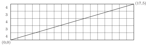
Figure 6. $c_{5/17}=100110110011011001$.

The next lemma, from [26], is essential for the definition of height.

Lemma 2.19.

$\left(c_{q}0\right)^{\infty}\in{\mathcal{KS}}$ for each rational $q\in(0,1/2]$. Moreover, the function $(0,1/2]\cap{\mathbb{Q}}\to{\mathcal{KS}}$ defined by $q\mapsto\left(c_{q}0\right)^{\infty}$ is strictly decreasing with respect to the unimodal order on ${\mathcal{KS}}$. ∎

Definition 2.20 (Height).

Let $\mu\in{\mathcal{KS}}$. Then the height $q(\mu)\in[0,1/2]$ of $\mu$ is given by

$$q(\mu)=\inf\left(\{q\in(0,1/2]\cap{\mathbb{Q}}\,:\,\left(c_{q}0\right)^{\infty}\prec\mu\}\cup\{1/2\}\right).$$

By Lemma 2.19, the height function $q\colon{\mathcal{KS}}\to[0,1/2]$ is decreasing with respect to the unimodal order on ${\mathcal{KS}}$ and the usual order on $[0,1/2]$. The next result, also from [26], describes the interval of kneading sequences with given rational height.

Definition 2.21 (The words $w_{q}$).

For each $q=m/n\in(0,1/2)$, define $w_{q}\in\{0,1\}^{n-1}$ to be the word obtained by deleting the last two symbols of $c_{q}$; and ${\widehat{w}}_{q}\in\{0,1\}^{n-1}$ to be the reverse of $w_{q}$.

Statements (a), (b), and (c) of the following lemma can be found in [26], while (d) is contained in results of [21] (see also Lemma 11.5 of [5] for a self-contained proof).

Lemma 2.22 (Characterization of kneading sequences of given height).

1. For each irrational $q\in[0,1/2]$, there is a unique $\mu\in{\mathcal{KS}}$ with $q(\mu)=q$, namely

   $$\mu=10^{\kappa_{1}(q)}110^{\kappa_{2}(q)}110^{\kappa_{3}(q)}11\ldots.$$

2. Let $\mu\in{\mathcal{KS}}$. Then $q(\mu)=0$ if and only if $\mu=10^{\infty}$; and $q(\mu)=1/2$ if and only if $\mu\preceq 101^{\infty}$.

3. Let $\mu\in{\mathcal{KS}}$ and $q=m/n\in(0,1/2)\cap{\mathbb{Q}}$. Then $q(\mu)=q$ if and only if

   $$\left(w_{q}1\right)^{\infty}\preceq\mu\preceq 10\left({\widehat{w}}_{q}1\right)^{\infty}.$$

   Moreover, if $q(\mu)=q$ and $\mu\not=\left(w_{q}1\right)^{\infty}$ then $c_{q}$ is an initial subword of $\mu$; and if $\mu$ is periodic, then either $\mu=\left(w_{q}1\right)^{\infty}$ or $\mu=\left(w_{q}0\right)^{\infty}$, or its period is at least $n+2$.

4. Let $q=m/n\in(0,1/2)\cap{\mathbb{Q}}$. then $10\left({\widehat{w}}_{q}1\right)^{\infty}$ is pre-periodic to $\left(w_{q}1\right)^{\infty}$: that is, there is some $r$ with $\sigma^{r}(10\left({\widehat{w}}_{q}1\right)^{\infty})=\left(w_{q}1\right)^{\infty}$. ∎

By Lemma 2.22 (b), Condition (a) of Convention 2.8 says exactly that $q(\kappa(f))\in[0,1/2)$.

The endpoints of the intervals of kneading sequences of given rational height will play an important role, as will the kneading sequences $\left(c_{q}0\right)^{\infty}$ used in the definition of height. The acronym NBT in the following notation stands for ‘no bogus transitions’ and reflects the original motivation of height.

Definitions 2.23 ($\operatorname{lhe}(q)$, $\operatorname{rhe}(q)$, $\operatorname{NBT}(q)$, ${\mathcal{KS}}(q)$).

Let $q\in(0,1/2)\cap{\mathbb{Q}}$. We write $\operatorname{lhe}(q)=\left(w_{q}1\right)^{\infty}$, $\operatorname{rhe}(q)=10\left({\widehat{w}}_{q}1\right)^{\infty}$, and $\operatorname{NBT}(q)=\left(c_{q}0\right)^{\infty}$. We write ${\mathcal{KS}}(q)$ for the set of kneading sequences $\mu$ with height $q$ (i.e. with $\operatorname{lhe}(q)\preceq\mu\preceq\operatorname{rhe}(q)$). In the special case $q=0$, we write $\operatorname{lhe}(q)=10^{\infty}$ and $\operatorname{rhe}(q)$ is undefined.

Example 2.24.

Let $q=2/7$, with $c_{q}=10011001$, $w_{q}=100110$, and ${\widehat{w}}_{q}=011001$. Then we have $\operatorname{lhe}(2/7)=\left(1001101\right)^{\infty}$, $\operatorname{rhe}(2/7)=10\left(0110011\right)^{\infty}$, and $\operatorname{NBT}(2/7)=\left(100110010\right)^{\infty}$. A kneading sequence $\mu$ lies in ${\mathcal{KS}}(2/7)$ if and only if $\left(1001101\right)^{\infty}\preceq\mu\preceq 10\left(0110011\right)^{\infty}$.

In addition to the characterization of Lemma 2.22, there is a straightforward algorithm which calculates $q(\mu)$ for any kneading sequence which has rational height: see Section 3.2 of [26]

As stated at the beginning of this section, the structure of the prime ends of $({\widehat{T}},{\widehat{I}})$ depends on whether $q(\kappa(f))$ is rational or irrational. The rational case $q(\kappa(f))=m/n$ also splits into two subcases: one in which $\kappa(f)$ is either an endpoint of ${\mathcal{KS}}(m/n)$ or is equal to $\left(w_{q}0\right)^{\infty}$ (a consecutive kneading sequence to $\operatorname{lhe}(m/n)$), and one in which neither of these happens. The endpoint case further splits into subcases which, while they yield the same results, are analyzed in quite different ways. These observations motivate the following definitions (see Figure 7).

Definitions 2.25 (Irrational and rational types; interior and endpoint types; early, strict, and late types; tent-like and quadratic-like types; normal type; general and NBT types).

We say that a unimodal map $f$ is of irrational type or of rational type according as $q(\kappa(f))$ is irrational or rational.

In the rational case, with $q(\kappa(f))=m/n\in(0,1/2)$, we say that $f$ is of (rational) endpoint type if $\kappa(f)\in\{\operatorname{lhe}(m/n),\left(w_{q}0\right)^{\infty},\operatorname{rhe}(m/n)\}$; and is of (rational) interior type otherwise.

In the rational endpoint case we say that $f$ is of left endpoint type if $\kappa(f)\in\{\operatorname{lhe}(m/n),\left(w_{q}0\right)^{\infty}\}$, and of right endpoint type if $\kappa(f)=\operatorname{rhe}(m/n)$.

In the rational left endpoint case, we say that $f$ is of early endpoint type if $\kappa(f)=\operatorname{lhe}(m/n)$ but $f^{n}(a)\not=a$; of strict endpoint type if $\kappa(f)=\operatorname{lhe}(m/n)$ and $f^{n}(a)=a$; and of late endpoint type if $\kappa(f)=\left(w_{q}0\right)^{\infty}$.

In the left strict endpoint case, we say that $f$ is of tent-like type if $b$ is the only period $n$ point of $f$ with itinerary $\operatorname{lhe}(m/n)$; and that it is of quadratic-like type if it has a second such period $n$ point (there cannot be more than two period $n$ points with this itinerary by Convention 2.8 (c)).

We say that $f$ is of normal (endpoint) type if it is either of right endpoint type, or of tent-like left strict endpoint type. (These are the only endpoint types which occur for tent maps.)

In the rational interior case we say that $f$ is of (rational) NBT type if $f^{n+2}(c)=c$ — in which case $\kappa(f)=\operatorname{NBT}(m/n)$ — and of (rational) general type otherwise.

In the special case $m/n=0$ (i.e. $\kappa(f)=10^{\infty}$), we declare $f$ to be of tent-like strict left endpoint type.

Remark 2.26.

To explain the terminology in the rational left endpoint case, consider a full monotonic family $\{f_{t}\}$ of unimodal maps such as the quadratic family, and let $t_{1}=\inf\{t\,:\,\kappa(f_{t})=\operatorname{lhe}(m/n)\}$. Then a saddle-node bifurcation occurs at $t=t_{1}$ creating a semi-stable period $n$ orbit, which contains a point of itinerary $\operatorname{lhe}(m/n)$ and attracts the orbit of the turning point. As $t$ increases, this periodic orbit splits into a stable-unstable pair of periodic orbits, both containing points of itinerary $\operatorname{lhe}(m/n)$. We follow this pair of periodic orbits until at $t=t_{2}$ the stable orbit contains the turning point. We still have $\kappa(f_{t_{2}})=\operatorname{lhe}(m/n)$, but now $f_{t_{2}}^{n}(a)=a$. When we increase the parameter further, the stable periodic orbit passes through the turning point and the kneading sequence becomes $\left(w_{q}0\right)^{\infty}$. Therefore $f_{t}$ is of early endpoint type for $t\in[t_{1},t_{2})$, of strict quadratic-like endpoint type for $t=t_{2}$, and of late endpoint type for $t>t_{2}$ sufficiently close to $t_{2}$. There is no corresponding distinction at the right hand endpoint of the height interval since, by Convention 2.8 (b), if $\kappa(f)=\operatorname{rhe}(m/n)$, which is not periodic, then $f(a)$ is necessarily periodic of period $n$ since it has the same itinerary $\left({\widehat{w}}_{q}1\right)^{\infty}$ as $f^{n+1}(a)$.

In the tent family, by contrast, $\kappa(f)=\operatorname{lhe}(m/n)$ only if $f^{n}(a)=a$, $\kappa(f)$ is never equal to $\left(c_{q}0\right)^{\infty}$, and there is only ever one point of any given itinerary. Therefore only the strict tent-like left hand endpoint case occurs. That is, only the first three rows of Figure 7 are relevant for tent maps.

The reason for the distinction between rational general and rational NBT types will become apparent in Section 5.

Figure 7. Types of unimodal maps.

3. The unwrapping

In this section we construct an explicit unwrapping $\overline{f}\colon T\to T$ of an arbitrary unimodal map $f\colon[a,b]\to[a,b]$. This construction provides explicit descriptions of the sphere ${\widehat{T}}$, the embedded inverse limit ${\widehat{I}}$, and the homeomorphism ${\widehat{H}}\colon{\widehat{T}}\to{\widehat{T}}$ which restricts to the natural extension ${\widehat{f}}$ on ${\widehat{I}}$.

The construction proceeds in two steps. In Section 3.1 we recall from [21] the outside map $B\colon S\to S$ corresponding to $f$, which is obtained by “fattening up” the interval to give it some two-dimensional structure (a closely related construction also appears in [17]). The unwrapping $\overline{f}$ itself is then constructed in Section 3.2. It is the product of the outside map and the identity on $\{(y,s)\,:\,s\leq 1/2\}\subset T$, and is gradually changed in $\{(y,s)\,:\,s\geq 1/2\}$ so that it satisfies the conditions of an unwrapping (Lemma 3.4). We finish with a description of the elements of ${\widehat{T}}\setminus{\widehat{I}}$ (Definition 3.6 and Lemma 3.7).

3.1. The outside map

Let $f\colon[a,b]\to[a,b]$ be a unimodal map with turning point $c\in(a,b)$. Recall that we denote by $\alpha$ the unique point of $(c,b]$ with $f(\alpha)=f(a)$.

Recall from Section 2.2 that $S$ denotes the circle obtained by gluing together two copies of $I$ at their endpoints; that points of $S$ are denoted $x_{u}$ or $x_{\ell}$ for $x\in I$; and that we write $a=a_{u}=a_{\ell}$ and $b=b_{u}=b_{\ell}\in S$. We will use standard interval notation $(x,y)$, $[x,y]$, etc. for subintervals of $S$, the interval consisting of the arc which goes counterclockwise, in the model of Figure 5, from the first point listed to the second. Thus, for example, the interval $[a,b]$ contains $x_{\ell}$ for all $x\in I$, while the interval $[b,a]$ contains $x_{u}$ for all $x\in I$.

The intuitive motivation for the definition of the outside map $B\colon S\to S$ is illustrated in Figure 8. We add some two-dimensional structure to the unimodal map $f$ as depicted on the left of the figure, regarding the image of $[a,c)$ as lying underneath the image of $(c,b]$. Then points which are above the interval, lying in $(a,\alpha)$, get folded into the interior – that is, they no longer remain on the outside. These points correspond to the interior of the interval $\gamma=[\alpha_{u},a]$ in $S$ depicted on the right hand side of the figure, which is collapsed to a point by the outside map. Other points above the interval, and all points below the interval, remain on the outside after one iteration, with points below $[a,c)$ and above $[\alpha,b]$ being sent below the interval, and points below $(c,b]$ being sent above the interval.

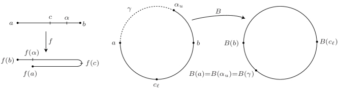
Figure 8. The outside map $B$ corresponding to a unimodal map $f$.

This intuition leads to the following definition:

Definition 3.1 (The outside map).

Let $f\colon[a,b]\to[a,b]$ be a unimodal map. The outside map $B\colon S\to S$ corresponding to $f$ is defined by

$$\begin{array}[]{rcll}B(x_{\ell})&=&f(x)_{\ell}&\text{ if }x\in[a,c]\\ B(x_{\ell})&=&f(x)_{u}&\text{ if }x\in[c,b]\\ B(x_{u})&=&f(x)_{\ell}&\text{ if }x\in[\alpha,b],\text{ and}\\ B(x_{u})&=&f(a)_{\ell}&\text{ for all }x\in[a,\alpha].\end{array}$$ (2)

The dynamics of the outside map plays a key role in the paper, and is discussed in detail in Section 4.4 below. For now we note that, by the first three equations of (2),

$$\tau\circ B(y)=f\circ\tau(y)\quad\text{ for all }y\in S\setminus{{\accentset{\circ}{\gamma}}},$$ (3)

where ${{\accentset{\circ}{\gamma}}}=(\alpha_{u},a)$ and $\tau\colon S\to I$ is the projection of Definition 2.11, satisfying $\tau(x_{\ell})=\tau(x_{u})=x$.

3.2. Definition of the unwrapping

We now use the outside map to define an unwrapping of the unimodal map $f$. Figure 9 shows the sphere $T$ (with $\partial$ opened out into the circle $S$), the interval $I\subset T$, the circle $S\times\{1/2\}$ (dashed line), and segments of some of the arcs $\eta_{y}$ (dotted lines). It also depicts an interval $J$ with endpoints $(f(a)_{\ell},\,1/2)$ and $(b,1)$. The unwrapping will be constructed so that as $x$ runs from $a$ to $c$, $\overline{f}(x_{\ell},1)$ runs along $J$ with $\Upsilon(\overline{f}(x_{\ell},1))=(f(x),1)$; while as $x$ runs from $c$ to $b$, $\overline{f}(x_{\ell},1)=(f(x),1)\in I$. The interval $J$ is defined by $J=\{(\phi(s)_{\ell},s)\,:\,s\in[1/2,1]\}$, where $\phi$ is the affine map of Definition 3.2 below.

Figure 9. Construction of the unwrapping $\overline{f}$.

Definition 3.2 (The map $\phi\colon[1/2,1]\to[f(a),b]$ and the unwrapping $\overline{f}$ of a unimodal map $f$).

Let $\phi\colon[1/2,1]\to[f(a),b]$ be the affine map

$$\phi(s)=f(a)+(2s-1)(b-f(a))$$

with $\phi(1/2)=f(a)$ and $\phi(1)=b$. We define $\overline{f}\colon T\to T$ as follows:

1. $\overline{f}(y,s)=(B(y),s)$ for all $(y,s)\in S\times[0,1/2]$.

2. If $y\in[c_{\ell},\alpha_{u}]$ then $\overline{f}(y,s)=(B(y),s)$ for all $s\in[0,1]$.

3. If $y\in[\alpha_{u},c_{u}]$ then

   $$\overline{f}(y,s)=\begin{cases}(\phi(s)_{\ell},s)&\text{ if }s\in[1/2,\,\,\phi^{-1}(f(\tau(y)))],\\ (f(\tau(y))_{\ell},s)&\text{ if }s\in[\phi^{-1}(f(\tau(y))),\,\,1].\end{cases}$$

4. If $y\in[c_{u},a]$ then

   $$\overline{f}(y,s)=\begin{cases}(\phi(s)_{\ell},s)&\text{ if }s\in[1/2,\,\,\phi^{-1}(f(\tau(y)))],\\ (f(\tau(y))_{\ell},\phi^{-1}(f(\tau(y)))&\text{ if }s\in[\phi^{-1}(f(\tau(y))),\,\,1].\end{cases}$$

5. If $y\in[a,c_{\ell}]$ then

   $$\overline{f}(y,s)=\begin{cases}(B(y),s)&\text{ if }s\in[1/2,\,\,\phi^{-1}(\tau(B(y)))],\\ (B(y),\phi^{-1}(\tau(B(y))))&\text{ if }s\in[\phi^{-1}(\tau(B(y))),\,\,1].\end{cases}$$

Remarks 3.3.

1. If $y\not\in{{\accentset{\circ}{\gamma}}}$ then the first component of $\overline{f}(y,s)$ is equal to $B(y)$ for all $s\in[0,1]$ by (U1), (U2), and (U5).

2. When parsing this definition, it is helpful to recall that, in order for $\overline{f}$ to be an unwrapping, we must have $\Upsilon(\overline{f}(y,1))=f(\tau(y))$ for each $y\in S$ (Definition 2.12 (b)). The value $s=\phi^{-1}(f(\tau(y)))$ which appears in (U3), (U4), and (U5) — noting that in (U5) we have $y\not\in{{\accentset{\circ}{\gamma}}}$, so that $\tau(B(y))=f(\tau(y))$ by (3) — is the parameter of the point $j_{y}$ of $J$ which retracts to $f(\tau(y))$: therefore $\overline{f}(y,1)$ must lie on the decomposition arc $\eta$ which passes through this point. According to the definition,

   1. When $y\in[\alpha_{u},c_{u}]$, the path $\{\overline{f}(y,s)\,:\,s\in[1/2,1]\}$ moves along $J$ from $(f(a)_{\ell},1/2)$ until it reaches $j_{y}$, and then moves along $\eta$ until it reaches $I$;

   2. When $y\in[c_{u},a]$, the path $\{\overline{f}(y,s)\,:\,s\in[1/2,1]\}$ moves along $J$ from $(f(a)_{\ell},1/2)$ until it reaches $j_{y}$, and then remains at this point;

   3. When $y\in[a,c_{\ell}]$, the path $\{\overline{f}(y,s)\,:\,s\in[1/2,1]\}$ moves along $\eta$ from $(B(y),1/2)$ until it reaches $j_{y}$, and then remains at this point.

Lemma 3.4.

$\overline{f}$ is an unwrapping of $f$.

Proof.

A theorem of Youngs [42] states that any continuous monotone surjection $T\to T$ is a near-homeomorphism. Therefore $\overline{f}$ is a near-homeomorphism (which is clearly orientation-preserving), since the preimage of each point of $T$ under $\overline{f}$ is either a point or an arc. In fact, the only points of $T$ whose preimages are not points are

• For each $s\in(0,1/2)$, the point $(f(a)_{\ell},s)$, whose preimage is the arc $[\alpha_{u},a]\times\{s\}$, and

• For each $s\in[1/2,1)$, the point $(\phi(s)_{\ell},s)$ of $J$, whose preimage is the arc

  $$[z(s)_{u},w(s)_{u}]\times\{s\}\,\,\cup\,\,\{w(s)_{u}\}\times[s,1]\,\,\cup\,\,\{w(s)_{\ell}\}\times[s,1],$$

  where $w(s)$ and $z(s)$ denote the points of $[a,c]$ and of $[c,b]$ respectively with $f(w(s))=f(z(s))=\phi(s)$. The first set in this union comes from (U3) and (U4), the second from (U4), and the third from (U5).

Moreover, $\overline{f}$ satisfies condition a) of Definition 2.12, since $\overline{f}|_{I}$ is injective, with $\overline{f}(y,1)\in I\cup J$ for all $y\in S$ by (U2) – (U5); it satisfies condition b) since $\Upsilon\circ\overline{f}(y,1)=f\circ\tau(y)$ for all $y\in S$ by (U2) – (U5) and (3); and it satisfies condition c) by (U1). It is therefore an unwrapping of $f$ as required. ∎

Definitions 3.5 ($H$, ${\widehat{T}}$, $U$, ${\widehat{H}}\colon{\widehat{T}}\to{\widehat{T}}$, ${\widehat{B}}\colon{\widehat{S}}\to{\widehat{S}}$).

As in Section 2.2, set $H=\Upsilon\circ\overline{f}\colon T\to T$, and observe that $H|_{I}=f$. Write

$${\widehat{T}} = \varprojlim(T,H)\quad\text{ (a topological sphere),}$$

$${\widehat{I}} = \varprojlim(I,H)=\varprojlim(I,f),\quad\text{ and}$$

$$U = {\widehat{T}}\setminus{\widehat{I}}.$$

Let ${\widehat{H}}\colon{\widehat{T}}\to{\widehat{T}}$ be the natural extension of $H\colon T\to T$, so that ${\widehat{H}}|_{{\widehat{I}}}={\widehat{f}}$, the natural extension of $f\colon I\to I$.

Let ${\widehat{B}}\colon{\widehat{S}}\to{\widehat{S}}$ denote the natural extension of the outside map $B\colon S\to S$. This is a circle homeomorphism, since ${\widehat{S}}$ is a topological circle by Brown’s theorem.

We next introduce some notation for the elements of $U$. The key fact here is that if $y\in S$ and $s\in[0,1/2)$, then $H(y,s)=\Upsilon\circ\overline{f}(y,s)=\Upsilon(B(y),s)=(B(y),2s)$. Recall that we denote by $\partial$ the element $\left<\partial,\partial,\ldots\right>$ of ${\widehat{T}}$.

Definition 3.6 (Threads ${\mathbf{T}}({\mathbf{y}},s)$ and ${\mathbf{T}}({\mathbf{y}},s,k)$ in $U$).

1. For each ${\mathbf{y}}\in{\widehat{S}}$ and $s\in(0,1)$, define

   $${\mathbf{T}}({\mathbf{y}},s)=\left<(y_{0},s),(y_{1},s/2),(y_{2},s/4),\ldots\right>\in U.$$ (4)

2. For each ${\mathbf{y}}\in{\widehat{S}}$, $s\in[1/2,1)$, and $k\geq 0$, define

   $${\mathbf{T}}({\mathbf{y}},s,k)=\left<f^{k}(H(y_{0},s)),\ldots,f(H(y_{0},s)),H(y_{0},s),(y_{0},s),(y_{1},s/2),(y_{2},s/4),\ldots\right>\in U.$$ (5)

Lemma 3.7.

Every element of $U\setminus\{\partial\}$ is equal to exactly one of the threads of Definition 3.6.

Proof.

Let ${\mathbf{x}}\in U\setminus\{\partial\}$. Since ${\mathbf{x}}\not\in{\widehat{I}}$, there is some least $k\geq 0$ with $x_{k}\not\in I$: therefore $x_{k}=(y,s)$ for some $y\in S$ and $s\in(0,1)$.

If $k=0$ then ${\mathbf{x}}={\mathbf{T}}({\mathbf{y}},s)$, where $y_{i}$ is the first component of $x_{i}$ for each $i$. On the other hand, if $k\geq 1$ then, since $H(x_{k})\in I$, we have $s\in[1/2,1)$; and ${\mathbf{x}}={\mathbf{T}}({\mathbf{y}},s,k-1)$ where $y_{i}$ is the first component of $x_{k+i}$ for each $i$. ∎

The interesting entry of the threads ${\mathbf{T}}({\mathbf{y}},s,k)$ is $H(y_{0},s)\in I$, which is where the transition takes place from the dynamics of the outside map to the dynamics of the unimodal map.

Remark 3.8.

The unwrapping $\overline{f}$ varies continuously with the unimodal map $f$. It follows from Theorem 2.14 that if $\{f_{t}\}$ is a continuously varying family of unimodal maps, then the spheres constructed above can be identified with a standard model in such a way that the homeomorphisms ${\widehat{H}}_{t}$ and the attractors ${\widehat{I}}_{t}$ vary continuously.

4. Calculation of prime ends

In this section we determine the prime ends of $({\widehat{T}},{\widehat{I}})$ for any unimodal map $f$ satisfying the conditions of Convention 2.8. The main tool that we use is an explicit homeomorphism $\Psi$ from the open disk $D={\widehat{S}}\times[0,\infty)/({\widehat{S}}\times\{0\})$ to $U={\widehat{T}}\setminus{\widehat{I}}$, which is defined in Section 4.1. We will see that $\Psi$ conjugates ${\widehat{H}}|_{U}$ to the product of ${\widehat{B}}$ and a simple push on $D$ (Corollary 4.10).

In Section 4.2 we define the locally uniformly landing set ${\mathcal{R}}$, a subset of ${\widehat{S}}$ with the property that $\Psi$ extends continuously over ${\mathcal{R}}\times\{\infty\}$. In Section 4.3 we impose some additional conditions (which we show later are always satisfied), and use these to construct a homeomorphism between ${\widehat{S}}$ and the circle ${\mathbb{P}}$ of prime ends.

The structure of the locally uniformly landing set for a specific unimodal map $f$ depends on the dynamics of the outside map $B\colon S\to S$, which is discussed in Section 4.4. Armed with the results of that section, we will be able to complete the calculation of prime ends. The details of this calculation depend on whether $f$ is of irrational type, of rational interior type, or of rational endpoint type, and these cases are presented in Sections 4.5, 4.6, and 4.7 respectively.

4.1. The homeomorphism $\Psi\colon D\to U$

Definitions 4.1 ($D$, $\overline{D}$, $\partial^{\prime}$, ${\widehat{S}}_{\infty}$, $X_{\infty}$, the push $\lambda$, the homeomorphisms $G\colon\overline{D}\to\overline{D}$ and $G\colon D\to D$).

Write $D={\widehat{S}}\times[0,\infty)/({\widehat{S}}\times\{0\})$ and $\overline{D}={\widehat{S}}\times[0,\infty]/({\widehat{S}}\times\{0\})$. We regard $D$ as a subset of $\overline{D}$, and use coordinates $({\mathbf{y}},s)\in{\widehat{S}}\times[0,\infty]$ on $D$ and $\overline{D}$: these coordinates are singular at $\partial^{\prime}$, the point corresponding to ${\widehat{S}}\times\{0\}$.

Write ${\widehat{S}}_{\infty}={\widehat{S}}\times\{\infty\}\subset\overline{D}$, the circle at infinity. Similarly, given any subset $X$ of ${\widehat{S}}$, we write $X_{\infty}=X\times\{\infty\}\subset{\widehat{S}}_{\infty}$.

Let $\lambda\colon[0,\infty]\to[0,\infty]$ be defined by

$$\lambda(s)=\begin{cases}2s&\text{ if }s\in[0,1],\\ s+1&\text{ if }s\in[1,\infty),\\ \infty&\text{ if }s=\infty,\end{cases}$$

and $G\colon\overline{D}\to\overline{D}$ be the homeomorphism defined by $G({\mathbf{y}},s)=({\widehat{B}}({\mathbf{y}}),\lambda(s))$. We denote the restriction to $D$ with the same symbol, $G\colon D\to D$.

In this section we define an explicit homeomorphism $\Psi\colon D\to U$, which is constructed in such a way that it conjugates $G\colon D\to D$ to ${\widehat{H}}\colon U\to U$, thereby providing a coordinate system on $U$ in which the action of ${\widehat{H}}$ is very easy to understand. We will see in subsequent sections that $\Psi$ extends over an open dense subset of the circle ${\widehat{S}}_{\infty}$ as a homeomorphism into ${\widehat{T}}$. The non-trivial prime ends of $({\widehat{T}},{\widehat{I}})$ can be understood in terms of the action of $\Psi$ on rays in $D$ which converge to points of ${\widehat{S}}_{\infty}$ at which $\Psi$ is discontinuous or not defined.

The surjectivity of $\Psi$ will be an immediate consequence of its definition (Lemma 4.7). To show that it is continuous and injective, we first establish that it semi-conjugates $G$ and ${\widehat{H}}$ (Lemma 4.8), and then use this semi-conjugacy to extend the obvious continuity and injectivity on ${\widehat{S}}\times(0,1)$ over the rest of $D$ (Corollary 4.9).

In order to define $\Psi$, it will be convenient to introduce the following notation (in which it should be noted carefully that $v$ is not the fractional part of $s$).

Definition 4.2 (Splitting $s$ into parts).

We define $P\colon[0,\infty)\to{\mathbb{N}}\times[1/2,1)$ by $P(s)=(t,v)$, where $t=\left\lfloor s\right\rfloor$ is the integer part of $s$ and $v=(u+1)/2$, where $u=s-t$ is the fractional part of $s$.

Definition 4.3 ($\Psi\colon D\to U$).

Define $\Psi\colon D\to U$ by $\Psi(\partial^{\prime})=\partial$ and

$$\Psi({\mathbf{y}},s)=\begin{cases}{\mathbf{T}}({\mathbf{y}},s)&\text{ if }s\in(0,1),\\ {\mathbf{T}}({\widehat{B}}^{-t}({\mathbf{y}}),v,t-1),&\text{ where $(t,v)=P(s)$, if $s\geq 1$.}\end{cases}$$ (6)

Substituting (5) into the formula for $\Psi({\mathbf{y}},s)$ in the case $s\geq 1$ yields the useful alternative expression

$$\Psi({\mathbf{y}},s)=\left<f^{t-1}(H(y_{t},v)),\ldots,f(H(y_{t},v)),H(y_{t},v),(y_{t},v),(y_{t+1},v/2),\ldots\right>\quad\text{ when }s\geq 1.$$ (7)

Therefore the number of entries of $\Psi({\mathbf{y}},s)$ which are in $I$ is equal to the integer part $t$ of $s$. We will frequently use the following immediate consequence of (7):

$$\Psi({\mathbf{y}},s)_{r}=f^{t-1-r}(H(y_{t},v))\qquad\text{for $0\leq r\leq t-1$, where $P(s)=(t,v)$}.$$ (8)

When $y\in\gamma$, the definition of $\overline{f}(y,s)$, and hence of $H(y,s)$, depends on whether $s$ is smaller or greater than $\phi^{-1}(f(\tau(y)))$ (see (U3) and (U4) of Definition 3.2). By (7), the behavior of $\Psi({\mathbf{y}},s)$ therefore depends on whether $v=(u+1)/2$ is smaller or greater than this value; that is, on whether the fractional part $u$ of $s$ is smaller or greater than $2\phi^{-1}(f(\tau(y_{t})))-1$. This value will frequently be significant in the remainder of the paper, and the following notation will be useful.

Definition 4.4 (The function $u\colon S\to[0,1]$).

Define $u\colon S\to[0,1]$ by

$$u(y)=\begin{cases}2\phi^{-1}(f(\tau(y)))-1&\text{ if }y\in\gamma,\\ 0&\text{ otherwise.}\end{cases}$$

In particular $u(c_{u})=1$ and $u(a)=u(\alpha_{u})=0$. The following lemma gives the key property of the function $u$.

Lemma 4.5.

Let $y\in S$ and $v\in[1/2,1)$, and write $u=2v-1\in[0,1)$. Then

$$H(y,v)=\begin{cases}f(\tau(y))&\text{ if }u\geq u(y),\\ \phi(v)&\text{ if }u<u(y).\end{cases}$$

Proof.

If $y\not\in\gamma$ then necessarily $u\geq u(y)$, and $H(y,v)=\tau(B(y))=f(\tau(y))$ by Remark 3.3 (a) and (3).

If $y\in\gamma$ and $u\geq u(y)$, then $v\geq\phi^{-1}(f(\tau(y)))$, and hence the first component of $\overline{f}(y,v)$ is $f(\tau(y))_{\ell}$ by (U3) and (U4) of Definition 3.2. Therefore $H(y,v)=\Upsilon\circ\overline{f}(y,v)=f(\tau(y))$ as required.

If $y\in\gamma$ and $u<u(y)$, then $v<\phi^{-1}(f(\tau(y)))$, and hence the first component of $\overline{f}(y,v)$ is $\phi(v)_{\ell}$ by (U3) and (U4) of Definition 3.2. Therefore $H(y,v)=\phi(v)$ as required. ∎

Remark 4.6.

If $y\in\gamma$ and $u=u(y)$ then $H(y,v)=f(\tau(y))=\phi(v)$. On the other hand, if $y\not\in\gamma$ and $u=u(y)=0$, then it need not be the case that $H(y,v)=\phi(v)$: we have $H(y,v)=f(\tau(y))$, while $\phi(v)=\phi(1/2)=f(a)$.

Lemma 4.7.

$\Psi\colon D\to U$ is surjective.

Proof.

Recall (Lemma 3.7) that every element of $U\setminus\{\partial\}$ is either of the form ${\mathbf{T}}({\mathbf{y}},s)$ for some ${\mathbf{y}}\in{\widehat{S}}$ and $s\in(0,1)$; or of the form ${\mathbf{T}}({\mathbf{y}},s,k)$ for some ${\mathbf{y}}\in{\widehat{S}}$, $s\in[1/2,1)$ and $k\geq 0$. In the former case we have ${\mathbf{T}}({\mathbf{y}},s)=\Psi({\mathbf{y}},s)$; while in the latter case ${\mathbf{T}}({\mathbf{y}},s,k)=\Psi({\widehat{B}}^{k+1}({\mathbf{y}}),k+1+(2s-1))$ by direct substitution into (6), since $P(k+1+(2s-1))=(k+1,s)$.

Since $\partial=\Psi(\partial^{\prime})$, this establishes the surjectivity of $\Psi$. ∎

Lemma 4.8.

${\widehat{H}}\circ\Psi=\Psi\circ G\colon D\to U$.

Proof.

The proof is a straightforward calculation by cases. Let $({\mathbf{y}},s)\in D$. If $s=0$ then $({\mathbf{y}},s)=\partial^{\prime}$, and ${\widehat{H}}(\Psi(\partial^{\prime}))=\Psi(G(\partial^{\prime}))=\partial$. We therefore assume that $s>0$.

1. If $s\in(0,1/2)$ then $H(y_{0},s)=\Upsilon\circ\overline{f}(y_{0},s)=(B(y_{0}),2s)$ by (U1) of Definition 3.2 and Definition 2.11. Therefore

   $${\widehat{H}}(\Psi({\mathbf{y}},s))={\widehat{H}}({\mathbf{T}}({\mathbf{y}},s))=\left<(B(y_{0}),2s),(y_{0},s),(y_{1},s/2),\ldots\right>={\mathbf{T}}({\widehat{B}}({\mathbf{y}}),2s)=\Psi(G({\mathbf{y}},s)).$$

2. If $s\in[1/2,1)$ then $P(\lambda(s))=P(2s)=P(1+(2s-1))=(1,s)$, so that

   $$\Psi(G({\mathbf{y}},s))=\Psi({\widehat{B}}({\mathbf{y}}),\lambda(s))={\mathbf{T}}({\widehat{B}}^{-1}({\widehat{B}}({\mathbf{y}})),s,0)={\mathbf{T}}({\mathbf{y}},s,0)=\left<H(y_{0},s),(y_{0},s),\ldots\right>={\widehat{H}}(\Psi({\mathbf{y}},s)).$$

3. If $s\in[1,\infty)$ then $\lambda(s)=s+1$, so that if $P(s)=(t,v)$ then $P(\lambda(s))=(t+1,v)$. Therefore

   $$\Psi(G({\mathbf{y}},s))=\Psi({\widehat{B}}({\mathbf{y}}),\lambda(s))={\mathbf{T}}({\widehat{B}}^{-(t+1)}({\widehat{B}}({\mathbf{y}})),v,t)={\mathbf{T}}({\widehat{B}}^{-t}({\mathbf{y}}),v,t)={\widehat{H}}(\Psi({\mathbf{y}},s)),$$

   since $H(f^{t-1}(H(y_{t},v)))=f^{t}(H(y_{t},v))$.

∎

Corollary 4.9.

$\Psi\colon D\to U$ is a homeomorphism.

Proof.

For each $N\geq 1$, the restriction of $G^{-N}$ to ${\widehat{S}}\times[0,N+1)$ is a homeomorphism onto ${\widehat{S}}\times[0,1)$. Lemma 4.8 gives

$$\Psi|_{{\widehat{S}}\times[0,N+1)}={\widehat{H}}^{N}\circ\Psi|_{{\widehat{S}}\times[0,1)}\circ G^{-N}|_{{\widehat{S}}\times[0,N+1)}.$$ (9)

Since $\Psi$ is evidently continuous and injective on ${\widehat{S}}\times[0,1)$, it is continuous and injective on ${\widehat{S}}\times[0,N+1)$ for each $N$, and hence on $D$. Therefore (using Lemma 4.7) $\Psi$ is a continuous bijection.

$\Psi^{-1}$ is clearly continuous on $\Psi({\widehat{S}}\times[0,1))$, and it is continuous on $\Psi({\widehat{S}}\times(0,\infty))$ by invariance of domain. ∎

Combining Lemma 4.8 and Corollary 4.9 gives:

Corollary 4.10.

$\Psi$ is a topological conjugacy between $G\colon D\to D$ and ${\widehat{H}}\colon U\to U$. ∎

4.2. Extension to the circle at infinity

We now investigate the extension of $\Psi$ to points $({\mathbf{y}},\infty)\in{\widehat{S}}_{\infty}$.

Definitions 4.11 (The rays $R_{\mathbf{y}}$, the landing set ${\mathcal{L}}$, the landing function $\omega\colon{\mathcal{L}}\to{\widehat{I}}$,  ${D^{{\scriptstyle\dagger}}}$, $\Psi\colon{D^{{\scriptstyle\dagger}}}\to{\widehat{T}}$).

For each ${\mathbf{y}}\in{\widehat{S}}$, let $R_{\mathbf{y}}\colon[0,\infty)\to U$ be the ray defined by $R_{{\mathbf{y}}}(s)=\Psi({\mathbf{y}},s)$. Define the landing set ${\mathcal{L}}\subset{\widehat{S}}$ to be the set of ${\mathbf{y}}\in{\widehat{S}}$ for which $R_{\mathbf{y}}$ lands; and let $\omega\colon{\mathcal{L}}\to{\widehat{I}}$ denote the landing function, which takes each ${\mathbf{y}}\in{\mathcal{L}}$ to the landing point of $R_{\mathbf{y}}$. We write ${D^{{\scriptstyle\dagger}}}=D\cup{\mathcal{L}}_{\infty}\subset\overline{D}$, and extend $\Psi\colon D\to U$ to a function $\Psi\colon{D^{{\scriptstyle\dagger}}}\to{\widehat{T}}$ by setting $\Psi({\mathbf{y}},\infty)=\omega({\mathbf{y}})$ for each ${\mathbf{y}}\in{\mathcal{L}}$.

The main results of this section are:

1. If all of the entries of the thread ${\mathbf{y}}$ after the $(N+1)^{\text{st}}$ lie in $S\setminus{{\accentset{\circ}{\gamma}}}$, then the first $N+1$ entries of the thread $\Psi({\mathbf{y}},s)$ are independent of $s$, provided that $s\geq N+1$ (Lemma 4.13). In particular (Corollary 4.14), ${\mathbf{y}}\in{\mathcal{L}}$. For this reason we say that an element ${\mathbf{y}}$ of ${\widehat{S}}$ satisfying this condition is landing of level $N$. We also show (Lemma 4.16) that the landing function $\omega$ is injective on the set of all points which are landing of some level.

2. If all threads sufficiently close to ${\mathbf{y}}$ are also landing of level $N$ (that is, if ${\mathbf{y}}$ has a locally uniformly landing neighborhood), then $\Psi$ is continuous at $({\mathbf{y}},\infty)$ (see Lemma 4.17 and Corollary 4.19).

Definitions 4.12 (Landing, ${\mathcal{L}}_{N}$, uniformly landing, locally uniformly landing set ${\mathcal{R}}$).

Let $N\in{\mathbb{N}}$. We say that ${\mathbf{y}}\in{\widehat{S}}$ is landing of level $N$ if $y_{i}\not\in{{\accentset{\circ}{\gamma}}}$ for all $i>N$; and we write ${\mathcal{L}}_{N}\subset{\widehat{S}}$ for the set of such points. (Therefore ${\mathcal{L}}_{0}\subset{\mathcal{L}}_{1}\subset{\mathcal{L}}_{2}\subset\cdots$.) We say that a subset $J$ of ${\widehat{S}}$ is uniformly landing (of level $N$) if $J\subset{\mathcal{L}}_{N}$. We write ${\mathcal{R}}$ for the set of elements of ${\widehat{S}}$ which have a uniformly landing neighborhood in ${\widehat{S}}$.

Lemma 4.13.

Let ${\mathbf{y}}\in{\mathcal{L}}_{N}$, and let $s\geq N+1$. Then, writing $P(s)=(t,v)$,

$$\Psi({\mathbf{y}},s)=\left<f^{N}(\tau(y_{N})),\ldots,f(\tau(y_{N})),\tau(y_{N}),\tau(y_{N+1}),\ldots,\tau(y_{t-2}),\tau(y_{t-1}),(y_{t},v),(y_{t+1},v/2),\ldots\right>.$$

Proof.

We have $t\geq N+1$. Now

$$\Psi({\mathbf{y}},s) = \left<f^{t-1}(H(y_{t},v)),\ldots,f(H(y_{t},v)),H(y_{t},v),(y_{t},v),(y_{t+1},v/2),\ldots\right>$$

$$= \left<f^{t-1}(\tau(y_{t-1})),\ldots,f(\tau(y_{t-1})),\tau(y_{t-1}),(y_{t},v),(y_{t+1},v/2),\ldots\right>$$

$$= \left<f^{N}(\tau(y_{N})),\ldots,f(\tau(y_{N})),\tau(y_{N}),\tau(y_{N+1}),\ldots,\tau(y_{t-2}),\tau(y_{t-1}),(y_{t},v),(y_{t+1},v/2),\ldots\right>$$

as required. Here the first equality is (7); for the second, we use Remark 3.3 (a) to give that $\overline{f}(y_{t},v)_{1}=B(y_{t})=y_{t-1}$, since $y_{t}\not\in{{\accentset{\circ}{\gamma}}}$, so that $H(y_{t},v)=\Upsilon(\overline{f}(y_{t},v))=\tau(y_{t-1})$; and for the third, we use that $f(\tau(y_{i}))=\tau(B(y_{i}))=\tau(y_{i-1})$ for all $i>N$ by (3), since $y_{i}\not\in{{\accentset{\circ}{\gamma}}}$ for these values of $i$. ∎

Corollary 4.14.

Let ${\mathbf{y}}\in{\mathcal{L}}_{N}$. Then ${\mathbf{y}}\in{\mathcal{L}}$ and

$$\omega({\mathbf{y}})=\left<f^{N}(\tau(y_{N})),\ldots,f(\tau(y_{N})),\tau(y_{N}),\tau(y_{N+1}),\tau(y_{N+2}),\ldots\right>.$$ (10)

In particular, ${\mathcal{R}}\subset{\mathcal{L}}$. ∎

Remark 4.15.

Therefore $\bigcup_{N\geq 0}{\mathcal{L}}_{N}\subset{\mathcal{L}}$. We will see later that these two sets are equal, except in the late left endpoint case: see Remark 4.70.

Lemma 4.16.

Let ${\mathcal{L}}^{\prime}=\bigcup_{N\geq 0}{\mathcal{L}}_{N}$. Then $\omega\colon{\mathcal{L}}^{\prime}\to{\widehat{I}}$ is injective.

Proof.

Let ${\mathbf{y}},{\mathbf{z}}\in{\mathcal{L}}^{\prime}$ be such that $\omega({\mathbf{y}})=\omega({\mathbf{z}})$. Pick $N$ such that ${\mathbf{y}},{\mathbf{z}}\in{\mathcal{L}}_{N}$. Then $\tau(y_{N+r})=\tau(z_{N+r})$ for all $r\geq 0$ by (10). However, at least one of any two successive entries of a thread of ${\widehat{I}}$ must lie in $[a,\alpha)$ (as $f([\alpha,b])=[a,f(a)]$, and $f(a)<\alpha$ since $\kappa(f)\succ 101^{\infty}$). Since $y_{N+r},z_{N+r}\not\in{{\accentset{\circ}{\gamma}}}$ for all $r$, it follows that $y_{N+r}=z_{N+r}$ for arbitrarily large $r$, so that ${\mathbf{y}}={\mathbf{z}}$ as required. ∎

Lemma 4.17.

Let $J$ be a uniformly landing subset of ${\widehat{S}}$. Then $\Psi|_{J\times[0,\infty]}$ is continuous.

Proof.

Since $\Psi$ is continuous on $D$ (Corollary 4.9), it suffices to prove continuity at points of $J_{\infty}$. So let ${\mathbf{y}}\in J$, and let $N$ be such that $J\subset{\mathcal{L}}_{N}$. Pick sequences ${\mathbf{y}}^{(i)}\to{\mathbf{y}}$ in $J$ and $s^{(i)}\to\infty$ in $[0,\infty)$.

Let $P(s^{(i)})=(t^{(i)},v^{(i)})$. Lemma 4.13 gives that, for sufficiently large $i$,

$$\Psi({\mathbf{y}}^{(i)},s^{(i)})=\left<f^{N}(\tau(y_{N}^{(i)})),\ldots,f(\tau(y_{N}^{(i)})),\tau(y_{N}^{(i)}),\tau(y_{N+1}^{(i)}),\ldots,\tau(y_{t^{(i)}-2}^{(i)}),\tau(y_{t^{(i)}-1}^{(i)}),(y_{t^{(i)}}^{(i)},v^{(i)}),\ldots\right>,$$

which converges to $\Psi({\mathbf{y}},\infty)=\omega({\mathbf{y}})$ as $i\to\infty$. Similarly, it follows from (10) that $\Psi({\mathbf{y}}^{(i)},\infty)\to\Psi({\mathbf{y}},\infty)$ as $i\to\infty$. ∎

If $J$ is uniformly landing but not open in ${\widehat{S}}$, then $\Psi$ (as opposed to its restriction to $J\times[0,\infty]$) may not be continuous at $({\mathbf{y}},\infty)$ when ${\mathbf{y}}$ is a boundary point of $J$. However, $\Psi$ is continuous at interior points of $J_{\infty}$, and in particular is continuous at $({\mathbf{y}},\infty)$ for all ${\mathbf{y}}$ in the locally uniformly landing set ${\mathcal{R}}$.

The following immediate corollary, which will be used frequently in the remainder of the paper, states that $\Psi$ extends continuously and injectively from the disk $D$ over the locally uniformly landing set at $\infty$. We will see later that this is the maximal set over which $\Psi$ has such an extension.

Definition 4.18 ($\widetilde{D}$).

We write $\widetilde{D}=D\cup{\mathcal{R}}_{\infty}\subset{D^{{\scriptstyle\dagger}}}\subset\overline{D}$.

Corollary 4.19.

$\Psi\colon\widetilde{D}\to{\widehat{T}}$ is injective and continuous. In particular, its restriction to any compact subset of $\widetilde{D}$ is a homeomorphism onto its image.

Proof.

$\Psi$ is injective since it is injective on $D$ and on ${\mathcal{R}}_{\infty}$ (Corollary 4.9 and Lemma 4.16), and $\Psi({\mathbf{y}},s)\in{\widehat{I}}$ if and only if $s=\infty$. It is continuous since it is continuous on $D$ (Corollary 4.9) and on ${\mathcal{R}}\times[0,\infty]$ (Lemma 4.17). ∎

So far in this section we have been concerned with the behavior of $\Psi({\mathbf{y}},s)$ as $s\to\infty$. Our final result is a technical lemma with a different flavor: it states that if there are several consecutive entries in a thread ${\mathbf{y}}$ which do not lie in ${{\accentset{\circ}{\gamma}}}$, then one entry (and hence all earlier entries) of the thread $\Psi({\mathbf{y}},s)$ is constant for $s$ in a corresponding interval.

Lemma 4.20.

Let ${\mathbf{y}}\in{\widehat{S}}$, and suppose that $r\geq 1$ and $k\geq 1$ are such that $y_{r+i}\not\in{{\accentset{\circ}{\gamma}}}$ for all $1\leq i\leq k$. Then

$$\Psi({\mathbf{y}},s)_{r-1}=f(\tau(y_{r}))\quad\text{ for all \ }s\in[r+u(y_{r}),\,r+k+1].$$

In particular, if ${\mathbf{y}}\in{\mathcal{L}}_{r}$, so that $y_{r+i}\not\in{{\accentset{\circ}{\gamma}}}$ for all $i\geq 1$, then $\Psi({\mathbf{y}},s)_{r-1}=f(\tau(y_{r}))$ for all $s\geq r+u(y_{r})$.

Proof.

Suppose first that $s\in[r+u(y_{r}),r+1)$, so that $P(s)=(r,v)$ for some $v\geq\frac{u(y_{r})+1}{2}$. Then $\Psi({\mathbf{y}},s)_{r-1}=H(y_{r},v)$ by (8); and $H(y_{r},v)=f(\tau(y_{r}))$ by Lemma 4.5.

Next suppose that $s\in[t,t+1)$ for some integer $t$ with $r+1\leq t\leq r+k$, so that $P(s)=(t,v)$ for some $v\in[1/2,1)$. Then $\Psi({\mathbf{y}},s)_{r-1}=f^{t-r}(H(y_{t},v))=f^{t-r}(\tau(B(y_{t})))=f^{t-r}(\tau(y_{t-1}))=f(\tau(y_{r}))$ as required. Here the first equality uses (8), the second uses Remark 3.3 (a), and the fourth uses (3) applied $t-r-1$ times.

That $\Psi({\mathbf{y}},r+k+1)_{r-1}=f(\tau(y_{r}))$ follows from the continuity of $\Psi$. ∎

4.3. Good chains of crosscuts

In this section we establish (Theorem 4.28) that there is a natural homeomorphism between ${\widehat{S}}$ and the circle ${\mathbb{P}}$ of prime ends of $({\widehat{T}},{\widehat{I}})$, with the property that, for each ${\mathbf{y}}\in{\widehat{S}}$, the ray $R_{{\mathbf{y}}}$ converges (in the sense of Section 1.2.4) to the prime end corresponding to ${\mathbf{y}}$. Moreover (Lemma 4.30), this homeomorphism conjugates the natural extension ${\widehat{B}}\colon{\widehat{S}}\to{\widehat{S}}$ of the outside map to the action of ${\widehat{H}}$ on ${\mathbb{P}}$, so that the prime end rotation number of $({\widehat{T}},{\widehat{I}})$ is equal to the Poincaré rotation number of ${\widehat{B}}$.

The arguments require two conditions which, while they always hold, we will only be able to establish, on a case by case basis, later. We therefore treat them as hypotheses for the time being. The first is that the locally uniformly landing set ${\mathcal{R}}$ is dense in ${\widehat{S}}$. The second is that there exist chains of crosscuts in $(\overline{D},{\widehat{S}}_{\infty})$ whose images under $\Psi$ are well-behaved chains of crosscuts in $({\widehat{T}},{\widehat{I}})$, as expressed by Definition 4.22 below. We carry over the definitions and notation of Section 1.2.4 to the (topologically trivial) pair $(\overline{D},{\widehat{S}}_{\infty})$: a crosscut in $(\overline{D},{\widehat{S}}_{\infty})$ is an arc $\xi^{\prime}$ in $\overline{D}$, disjoint from $\partial^{\prime}$, which intersects ${\widehat{S}}_{\infty}$ exactly at its endpoints; $U(\xi^{\prime})$ denotes the component of $D\setminus\xi^{\prime}$ which doesn’t contain $\partial^{\prime}$; $\xi_{2}^{\prime}<\xi_{1}^{\prime}$ means that $U(\xi_{2}^{\prime})\subset U(\xi_{1}^{\prime})$; and $(\xi_{k}^{\prime})$ is a chain of crosscuts in $(\overline{D},{\widehat{S}}_{\infty})$ if the $\xi_{k}^{\prime}$ are disjoint crosscuts with $\xi^{\prime}_{k+1}<\xi^{\prime}_{k}$ for each $k$ and $\operatorname{diam}(\xi_{k}^{\prime})\to 0$ as $k\to\infty$.

Remark 4.21.

If a crosscut $\xi_{k}^{\prime}$ in $(\overline{D},{\widehat{S}}_{\infty})$ has endpoints in ${\mathcal{R}}_{\infty}$ then, by Corollary 4.19, $\Psi|_{\xi_{k}^{\prime}}$ is a homeomorphism onto its image $\xi_{k}$, which is therefore a crosscut in $({\widehat{T}},{\widehat{I}})$.

Definition 4.22 (Good chain of crosscuts).

Let ${\mathbf{y}}\in{\widehat{S}}$. A chain $(\xi^{\prime}_{k})$ of crosscuts in $(\overline{D},{\widehat{S}}_{\infty})$ is called a good chain for ${\mathbf{y}}$ if

1. The endpoints of each $\xi^{\prime}_{k}$ are in ${\mathcal{R}}_{\infty}$, so that $\xi_{k}=\Psi(\xi_{k}^{\prime})$ is a crosscut in $({\widehat{T}},{\widehat{I}})$ by Remark 4.21;

2. $({\mathbf{y}},\infty)\in\overline{U(\xi_{k}^{\prime})}$ for each $k$, so in particular $\xi_{k}^{\prime}\to({\mathbf{y}},\infty)$ as $k\to\infty$;

3. $\operatorname{diam}(\xi_{k})\to 0$ as $k\to\infty$; and

4. if ${\mathbf{y}}\not\in{\mathcal{L}}$, then $(\xi_{k})$ does not converge to a point ${\mathbf{x}}$ of ${\widehat{I}}$.

Remarks 4.23.

1. By Definition 4.22 (a) and (c), if $(\xi^{\prime}_{k})$ is a good chain of crosscuts for ${\mathbf{y}}$, then $(\xi_{k})$ is a chain of crosscuts in $({\widehat{T}},{\widehat{I}})$.

2. Suppose that there is a good chain of crosscuts $(\xi^{\prime}_{k})$ for ${\mathbf{y}}\in{\widehat{S}}$.

   • If ${\mathbf{y}}\in{\mathcal{L}}$ then, since $R_{{\mathbf{y}}}$ lands at $\omega({\mathbf{y}})$ and intersects every $\xi_{k}$, we have $\xi_{k}\to\omega({\mathbf{y}})$ as $k\to\infty$. It follows that for every ray $\sigma^{\prime}\colon[0,\infty)\to D$ which lands at $({\mathbf{y}},\infty)$, the ray $\sigma=\Psi\circ\sigma^{\prime}$ either lands at $\omega({\mathbf{y}})$, or does not land.

   • If ${\mathbf{y}}\not\in{\mathcal{L}}$, then for every such ray $\sigma^{\prime}$, the ray $\sigma=\Psi\circ\sigma^{\prime}$ intersects $\xi_{k}$ for all sufficiently large $k$, and therefore does not land, by condition (d) of the definition.

3. By Corollary 4.19, there is a good chain of crosscuts for every ${\mathbf{y}}\in{\mathcal{R}}$.

4. We will continue to use the notational convention introduced above: functions $f^{\prime}\colon X\to\widetilde{D}$ and subsets $Y^{\prime}\subset\widetilde{D}$ will be denoted with primed symbols, and the corresponding functions $f=\Psi\circ f^{\prime}\colon X\to{\widehat{T}}$ and subsets $Y=\Psi(Y^{\prime})\subset{\widehat{T}}$ with the corresponding unprimed symbols.

Lemma 4.24.

Suppose that ${\mathcal{R}}$ is dense in ${\widehat{S}}$, and let $\sigma\colon[0,\infty)\to U$ be a ray which lands at a point of ${\widehat{I}}$. Then the ray $\sigma^{\prime}=\Psi^{-1}\circ\sigma$ lands at a point of ${\widehat{S}}_{\infty}$.

Proof.

The remainder $\operatorname{Rem}(\sigma^{\prime})$ is a connected subset of ${\widehat{S}}_{\infty}$, so if $\sigma^{\prime}$ didn’t land then, since ${\mathcal{R}}$ is open and dense in ${\widehat{S}}$, there would be a non-trivial closed subinterval $J$ of ${\mathcal{R}}$ with $J_{\infty}\subset\operatorname{Rem}(\sigma^{\prime})$. This would contradict the fact that $\sigma$ lands, since $\Psi|_{J\times[0,\infty]}$ is a homeomorphism onto its image by Corollary 4.19. ∎

Corollary 4.25.

Suppose that ${\mathcal{R}}$ is dense in ${\widehat{S}}$. If $\xi$ is a crosscut in $({\widehat{T}},{\widehat{I}})$, then $\xi^{\prime}=\Psi^{-1}(\xi)$ is a crosscut in $(\overline{D},{\widehat{S}}_{\infty})$. Moreover, if $\xi_{2}<\xi_{1}$ are crosscuts in $({\widehat{T}},{\widehat{I}})$, then $\xi_{2}^{\prime}<\xi_{1}^{\prime}$

Proof.

Immediate from Lemma 4.24 and the fact that $U(\xi^{\prime})=\Psi^{-1}(U(\xi))$. ∎

We now associate a point of ${\widehat{S}}$ with each prime end ${\mathcal{P}}$ in $({\widehat{T}},{\widehat{I}})$, under the assumption that ${\mathcal{R}}$ is dense in ${\widehat{S}}$. Suppose that ${\mathcal{P}}$ is represented by a chain $(\xi_{k})$, and write $U_{k}=U(\xi_{k})$. Then each $\xi_{k}^{\prime}=\Psi^{-1}(\xi_{k})$ is a crosscut in $(\overline{D},{\widehat{S}}_{\infty})$, and $U_{k}^{\prime}:=U(\xi_{k}^{\prime})=\Psi^{-1}(U_{k})$.

Let $J_{k}^{\prime}=\overline{U_{k}^{\prime}}\cap{\widehat{S}}_{\infty}$, a compact arc with endpoints the endpoints of $\xi_{k}^{\prime}$. Then $\bigcap_{k\geq 0}J_{k}^{\prime}$ is a single point. For if not then, since ${\mathcal{R}}$ is open and dense in ${\widehat{S}}$, the intersection would contain $K_{\infty}$ for some $K=[{\mathbf{y}}_{1},{\mathbf{y}}_{2}]\subset{\mathcal{R}}$, and every $\xi_{k}$ would intersect both $\Psi(\{{\mathbf{y}}_{1}\}\times[0,\infty])$ and $\Psi(\{{\mathbf{y}}_{2}\}\times[0,\infty])$, contradicting $\operatorname{diam}(\xi_{k})\to 0$ as $\Psi|_{K\times[0,\infty]}$ is a homeomorphism onto its image by Corollary 4.19.

Since the point of $\bigcap_{k\geq 0}J_{k}^{\prime}$ is independent of the choice of chain representing ${\mathcal{P}}$, we can make the following definition:

Definition 4.26 (${\mathbf{y}}\colon{\mathbb{P}}\to{\widehat{S}}$).

Suppose that ${\mathcal{R}}$ is dense in ${\widehat{S}}$. Let ${\mathcal{P}}$ be a prime end of $({\widehat{T}},{\widehat{I}})$. We write ${\mathbf{y}}({\mathcal{P}})$ for the element of ${\widehat{S}}$ defined by

$$\bigcap_{k\geq 0}\left(\overline{\Psi^{-1}(U(\xi_{k}))}\cap{\widehat{S}}_{\infty}\right)=\{({\mathbf{y}}({\mathcal{P}}),\infty)\},$$

where $(\xi_{k})$ is a chain representing ${\mathcal{P}}$.

Lemma 4.27.

Suppose that ${\mathcal{R}}$ is dense in ${\widehat{S}}$. Then ${\mathbf{y}}\colon{\mathbb{P}}\to{\widehat{S}}$ is continuous.

Proof.

Let $J$ be an open subset of ${\widehat{S}}$, and let ${\mathcal{P}}\in{\mathbf{y}}^{-1}(J)$ be represented by a chain $(\xi_{k})$. Then there is some $k$ such that $\overline{\Psi^{-1}(U(\xi_{k}))}\cap{\widehat{S}}_{\infty}\subset J$, and we have ${\mathcal{P}}\in{\mathcal{B}}(\xi_{k})\subset{\mathbf{y}}^{-1}(J)$, where ${\mathcal{B}}(\xi_{k})$ is the basic open subset defined in Section 1.2.4. ∎

Theorem 4.28.

Suppose that ${\mathcal{R}}$ is dense in ${\widehat{S}}$, and that there is a good chain of crosscuts for every ${\mathbf{y}}\in{\widehat{S}}$. Then

1. ${\mathbf{y}}\colon{\mathbb{P}}\to{\widehat{S}}$ is a homeomorphism;

2. For each ${\mathbf{y}}\in{\widehat{S}}$, the unique prime end ${\mathcal{P}}$ with ${\mathbf{y}}({\mathcal{P}})={\mathbf{y}}$ is defined by the chain $(\Psi(\xi_{k}^{\prime}))$, where $(\xi_{k}^{\prime})$ is any good chain of crosscuts for ${\mathbf{y}}$: or, indeed, any chain of crosscuts which satisfies (a) – (c) of Definition 4.22.

3. For each ${\mathbf{y}}\in{\widehat{S}}$, the ray $R_{\mathbf{y}}$ converges to the unique prime end ${\mathcal{P}}$ with ${\mathbf{y}}({\mathcal{P}})={\mathbf{y}}$; and

4. the set of accessible points of ${\widehat{I}}$ is $\{\omega({\mathbf{y}})\,:\,{\mathbf{y}}\in{\mathcal{L}}\}$.

Proof.

1. Let ${\mathbf{y}}\in{\widehat{S}}$, and let $(\xi_{k}^{\prime})$ be a good chain of crosscuts for ${\mathbf{y}}$. Write $U_{k}^{\prime}=U(\xi_{k}^{\prime})$, $\xi_{k}=\Psi(\xi_{k}^{\prime})$, and $U_{k}=U(\xi_{k})=\Psi(U_{k}^{\prime})$. By Remark 4.23 (a), $(\xi_{k})$ is a chain of crosscuts in $({\widehat{T}},{\widehat{I}})$, which therefore represents a prime end ${\mathcal{P}}\in{\mathbb{P}}$. By condition (b) of Definition 4.22 we have ${\mathbf{y}}({\mathcal{P}})={\mathbf{y}}$. In particular, ${\mathbf{y}}\colon{\mathbb{P}}\to{\widehat{S}}$ is surjective.

   To show injectivity, suppose that $(\Xi_{k})$ is another chain of crosscuts in $({\widehat{T}},{\widehat{I}})$ which defines a prime end ${\mathcal{Q}}\in{\mathbb{P}}$ with ${\mathbf{y}}({\mathcal{Q}})={\mathbf{y}}({\mathcal{P}})={\mathbf{y}}$. Write $V_{k}=U(\Xi_{k})$, and $V_{k}^{\prime}=\Psi^{-1}(V_{k})$. By Corollary 4.25, each $\Xi^{\prime}_{k}=\Psi^{-1}(\Xi_{k})$ is a crosscut in $(\overline{D},{\widehat{S}}_{\infty})$. In order to show that ${\mathcal{Q}}={\mathcal{P}}$, we need to show that each $V_{\ell}$ contains all but finitely many $U_{k}$, and each $U_{\ell}$ contains all but finitely many $V_{k}$.

   Now for each $\ell$, since ${\mathbf{y}}({\mathcal{Q}})={\mathbf{y}}$, we have that $\overline{V_{\ell}^{\prime}}$ contains an arc $J_{\ell}^{\prime}$ in ${\widehat{S}}_{\infty}$ with $({\mathbf{y}},\infty)\in J_{\ell}^{\prime}$. Moreover, since the $\Xi_{k}$ are mutually disjoint, so are the $\Xi_{k}^{\prime}$ by Remark 4.23 (b) (this is where we use condition (d) of Definition 4.22). Therefore $({\mathbf{y}},\infty)$ cannot be an endpoint of more than one of the crosscuts $\Xi^{\prime}_{k}$, and hence is in the interior of $J_{\ell}^{\prime}$. Since $\xi_{k}^{\prime}\to({\mathbf{y}},\infty)$, it follows that $U_{k}^{\prime}\subset V_{\ell}^{\prime}$ — and hence $U_{k}\subset V_{\ell}$ — for all sufficiently large $k$.

   To show that each $U_{\ell}$ contains all but finitely many $V_{k}$, let $\xi^{\prime}<\xi_{\ell}^{\prime}$ be a crosscut disjoint from $\xi_{\ell}^{\prime}$ whose endpoints are in the same components of ${\mathcal{R}}_{\infty}$ as the endpoints of $\xi_{\ell}^{\prime}$, and which satisfies $({\mathbf{y}},\infty)\in\overline{U(\xi^{\prime})}$. Let $X$ be the compact subset of $\overline{D}$ bounded by $\xi_{\ell}^{\prime}$ and $\xi^{\prime}$. Since $\Psi|_{X}$ is a homeomorphism onto its image, arcs which intersect both $\Psi(U(\xi^{\prime}))$ and the complement of $\Psi(U_{\ell}^{\prime})$ have diameter bounded below. Now $\Xi_{k}$ intersects $\Psi(U(\xi^{\prime}))$ for all sufficiently large $k$ (since ${\mathbf{y}}({\mathcal{Q}})={\mathbf{y}}$), and $\operatorname{diam}(\Xi_{k})\to 0$, so that $\operatorname{Int}(\Xi_{k})\subset\Psi(U_{\ell}^{\prime})=U_{\ell}$ — and hence $V_{k}\subset U_{\ell}$ — for all sufficiently large $k$ as required.

2. Follows immediately from the first paragraph of the proof of (a), which doesn’t make use of condition (d) of Definition 4.22.

3. For each $k$ there is some $t$ with $\{{\mathbf{y}}\}\times[t,\infty)\subset U(\xi_{k}^{\prime})$, and therefore

   $$R_{{\mathbf{y}}}([t,\infty))=\Psi(\{{\mathbf{y}}\}\times[t,\infty))\subset\Psi(U(\xi_{k}^{\prime}))=U(\Psi(\xi_{k}^{\prime})),$$

   so that $R_{{\mathbf{y}}}$ converges to the prime end defined by the chain $(\Psi(\xi_{k}^{\prime}))$ as required.

4. Clearly $\omega({\mathbf{y}})$ is accessible for all ${\mathbf{y}}\in{\mathcal{L}}$, since it is the landing point of the ray $R_{\mathbf{y}}$.

   Let ${\mathbf{x}}$ be an accessible point of ${\widehat{I}}$, so that there is a ray $\sigma\colon[0,\infty)\to U$ which lands at ${\mathbf{x}}$. By Lemma 4.24, the ray $\sigma^{\prime}=\Psi^{-1}\circ\sigma$ lands at some $({\mathbf{y}},\infty)\in{\widehat{S}}_{\infty}$. By Remark 4.23 (b), ${\mathbf{y}}\in{\mathcal{L}}$ and ${\mathbf{x}}=\omega({\mathbf{y}})$.

∎

Definition 4.29 (${\mathcal{P}}\colon{\widehat{S}}\to{\mathbb{P}}$).

Suppose that ${\mathcal{R}}$ is dense in ${\widehat{S}}$, and that there is a good chain of crosscuts for every ${\mathbf{y}}\in{\widehat{S}}$. Then we write ${\mathcal{P}}\colon{\widehat{S}}\to{\mathbb{P}}$ for the inverse of the homeomorphism ${\mathbf{y}}\colon{\mathbb{P}}\to{\widehat{S}}$.

Lemma 4.30.

Suppose that ${\mathcal{R}}$ is dense in ${\widehat{S}}$, and that there is a good chain of crosscuts for every ${\mathbf{y}}\in{\widehat{S}}$. Then ${\mathcal{P}}\colon{\widehat{S}}\to{\mathbb{P}}$ conjugates ${\widehat{B}}\colon{\widehat{S}}\to{\widehat{S}}$ to ${\widehat{H}}\colon{\mathbb{P}}\to{\mathbb{P}}$. In particular, the prime end rotation number of ${\widehat{H}}\colon({\widehat{T}},{\widehat{I}})\to({\widehat{T}},{\widehat{I}})$ is equal to $\rho({\widehat{B}})$.

Proof.

Let ${\mathbf{y}}\in{\widehat{S}}$. By Theorem 4.28 (c), the ray $R_{\mathbf{y}}$ converges to ${\mathcal{P}}({\mathbf{y}})$, and hence ${\widehat{H}}\circ R_{\mathbf{y}}$ converges to ${\widehat{H}}({\mathcal{P}}({\mathbf{y}}))$. By Lemma 4.8, ${\widehat{H}}\circ R_{{\mathbf{y}}}(s)=R_{{\widehat{B}}({\mathbf{y}})}(\lambda(s))$, so that the image of ${\widehat{H}}\circ R_{\mathbf{y}}$ coincides with the image of $R_{{\widehat{B}}({\mathbf{y}})}$, which converges to ${\mathcal{P}}({\widehat{B}}({\mathbf{y}}))$ by Theorem 4.28 (c). Therefore ${\widehat{H}}({\mathcal{P}}({\mathbf{y}}))={\mathcal{P}}({\widehat{B}}({\mathbf{y}}))$ as required. ∎

We will see later (Corollary 4.36) that $\rho({\widehat{B}})=\rho(B)=q(\kappa(f))$. The following lemma summarizes those parts of the results above which are relevant to the classification of prime ends, for future reference.

Lemma 4.31.

Suppose that ${\mathcal{R}}$ is dense in ${\widehat{S}}$, and that there is a good chain of crosscuts for every ${\mathbf{y}}\in{\widehat{S}}$. Then

1. If ${\mathbf{y}}\in{\mathcal{L}}$ then $\Pi({\mathcal{P}}({\mathbf{y}}))=\{\omega({\mathbf{y}})\}$.

2. If ${\mathbf{y}}\in{\mathcal{R}}$ then ${\mathcal{I}}({\mathcal{P}}({\mathbf{y}}))=\{\omega({\mathbf{y}})\}$.

In particular, a prime end ${\mathcal{P}}\in{\mathbb{P}}$ is of the first kind if ${\mathbf{y}}({\mathcal{P}})\in{\mathcal{R}}$; and is of the first or second kind if ${\mathbf{y}}({\mathcal{P}})\in{\mathcal{L}}$.

Proof.

(a) follows from the fact that $R_{\mathbf{y}}$ converges to ${\mathcal{P}}({\mathbf{y}})$ and lands at $\omega({\mathbf{y}})$ (see Section 1.2.4). (b) is immediate from the homeomorphism established in Corollary 4.19. ∎

4.4. Dynamics of the outside map

In order to determine the prime ends of $({\widehat{T}},{\widehat{I}})$, it suffices, in view of the homeomorphism between ${\mathbb{P}}$ and ${\widehat{S}}$ (Theorem 4.28) and the triviality of prime ends ${\mathcal{P}}({\mathbf{y}})$ with ${\mathbf{y}}\in{\mathcal{R}}$ (Lemma 4.31), to prove that ${\mathcal{R}}$ is dense in ${\widehat{S}}$ and that there is a good chain of crosscuts for every ${\mathbf{y}}\in{\widehat{S}}$; and then to analyze the prime ends which the rays $R_{{\mathbf{y}}}$ converge to in the cases when ${\mathbf{y}}\not\in{\mathcal{R}}$. The arguments and conclusions are quite different depending on whether $f$ is of rational or irrational type, and we will consider these cases separately.

In this section we state and prove the main result which will be needed about the dynamics of the outside map $B\colon S\to S$. Because the locally uniformly landing set ${\mathcal{R}}$ of Definitions 4.12 depends on occurrences of elements of ${{\accentset{\circ}{\gamma}}}$ in the threads ${\mathbf{y}}\in{\widehat{S}}$, it is primarily necessary to understand the recurrence properties of $\gamma$. Since $B$ collapses $\gamma$ to the single point $B(a)$, the main question is: when does the orbit of $B(a)$ first enter $\gamma$? We will see that if $f$ is of rational type with $q(\kappa(f))=m/n$, then $n$ is the smallest positive integer with $B^{n}(a)\in\gamma$, except when $f$ is of early left endpoint type; while if $f$ is of irrational type, or of early left endpoint type, then the orbit of $B(a)$ is disjoint from $\gamma$.

Definition 4.32 ($N(f)$).

Let $f\colon[a,b]\to[a,b]$ be a unimodal map, and $B\colon S\to S$ be the corresponding outside map. We define $N(f)\in{\mathbb{N}}\cup\{\infty\}$ by $N(f)=\infty$ if $B^{r}(a)\not\in\gamma$ for all $r\geq 1$, and otherwise

$$N(f)=\min\{r\geq 1\,:\,B^{r}(a)\in\gamma\}.$$

Theorem 4.33 below is an extension (both to more general hypotheses and to stronger conclusions) of a result of [21]. Because of the central role which this theorem plays in the paper, we prove it in full, although we do rely on some technical lemmas from [21].

Before stating the theorem, we remark that the outside map $B\colon S\to S$ is a monotone degree 1 circle map, and therefore has a Poincaré rotation number $\rho(B)$. Recall that we denote by $\alpha$ the unique element of $(c,b]$ with $f(\alpha)=f(a)$. The reader is encouraged to review the notation and results of Section 2.4 before proceeding.

Theorem 4.33 (Dynamics of the outside map).

Let $f\colon[a,b]\to[a,b]$ be a unimodal map with kneading sequence $\kappa(f)=\mu$, and let $B\colon S\to S$ be the corresponding outside map. Then

1. $\rho(B)=q(\mu)$.

2. If $q(\mu)=m/n$ is rational and $f$ is not of early left endpoint type, then

   1. $N(f)=n$;

   2. $B^{n}(a)=a\iff\mu=\operatorname{lhe}(m/n)$ and $B^{n}(a)=\alpha_{u}\iff\mu=\operatorname{rhe}(m/n)$; and

   3. The set $S\setminus\bigcup_{r\geq 0}B^{-r}(\gamma)$ of points whose orbits never fall into $\gamma$ is:

      • empty if $f$ is of normal endpoint type;

      • the union of $n$ half-open intervals, with open endpoint at a point of the orbit of $B(a)$ and closed endpoint at a point of a second period $n$ orbit of $B$, if $f$ is of quadratic-like strict left endpoint type; and

      • a single period $n$ orbit of $B$ otherwise.

3. If $q(\mu)=m/n$ is rational and $f$ is of early left endpoint type, then

   1. $N(f)=\infty$; and

   2. $B$ has a period $n$ orbit $Q$ disjoint from $\gamma$ which attracts the orbit of $B(a)$.

4. If $q(\mu)$ is irrational, then

   1. $N(f)=\infty$;

   2. The set $\bigcup_{r\geq 0}B^{-r}(\gamma)$ of points whose orbits fall into $\gamma$ is dense in $S$; and

   3. The orbit $\{B^{r}(a)\,:\,r\geq 1\}$ of $B(a)$ is dense in $S\setminus\bigcup_{r\geq 0}B^{-r}(\gamma)$.

We will use two lemmas. The first, Lemma 4.34 below, provides tools for determining $N(f)$ and the rotation number $\rho(B)$. Although the lemma is straightforward, its statement may be hard to parse, and we start with an informal description. For $r\leq N(f)$ we have that $\tau(B^{r}(a))=f^{r}(a)$ by (3). In order to determine whether or not $B^{r}(a)\in\gamma$, we need to decide whether $B^{r}(a)$ is equal to $f^{r}(a)_{u}$ or to $f^{r}(a)_{\ell}$; and, in the former case, whether or not $f^{r}(a)\leq\alpha$. The set ${\mathcal{J}}$ defined in the statement of the lemma has the property that, for $1\leq r\leq N(f)$, $B^{r}(a)=f^{r}(a)_{u}$ if and only if $r\in{\mathcal{J}}$. Since $\iota(f^{r}(a))=\sigma^{r+1}(\kappa(f))$ and $\iota(\alpha)=1\sigma^{2}(\kappa(f))$, the smallest $r$ with $B^{r}(a)\in\gamma$ is equal to the smallest $r$ for which $r\in{\mathcal{J}}$ and $\sigma^{r+1}(\kappa(f))\preceq 1\sigma^{2}(\kappa(f))$: this is the content of parts (a) and (b). We will see that $\rho(B)$ depends on how many points of the orbit of $B(a)$ lie in the upper half of the circle, and part (c) of the lemma enables us to calculate this. Finally, part (d) extends the ideas of (a) and (b) to give conditions under which there is a periodic orbit of $B$, disjoint from $\gamma$, above a periodic orbit of $f$.

Lemma 4.34.

Let $f\colon[a,b]\to[a,b]$ be a unimodal map with kneading sequence $\kappa(f)=\mu$, and let $B\colon S\to S$ be the corresponding outside map. Write

$${\mathcal{J}}=\{r\in{\mathbb{N}}\,:\,\text{there is some $0\leq k\leq(r-1)/2$ such that }\sigma^{r-(2k+1)}(\mu)=01^{2k+1}\sigma^{r+1}(\mu)\}.$$ (11)

1. Suppose that $\sigma^{r+1}(\mu)\succ 1\sigma^{2}(\mu)$ for all $r\in{\mathcal{J}}$. Then $N(f)=\infty$, provided that $c$ is not a periodic point of $f$.

2. Otherwise, let $r$ be least such that $r\in{\mathcal{J}}$ and $\sigma^{r+1}(\mu)\preceq 1\sigma^{2}(\mu)$. Then $N(f)=r$, provided that $f^{i}(a)\not=c$ for $1\leq i<r$.

3. For each $N\leq N(f)$ we have

   $$\#\,\{r\leq N\,:\,B^{r}(a)=f^{r}(a)_{u}\}=\#\,\{r\leq N\,:\,r\in{\mathcal{J}}\},$$

   provided that $f^{i}(a)\not=c$ for $1\leq i<N(f)$.

4. Suppose that $f$ has a period $N$ point $x$ whose orbit does not contain $c$; and that $\iota(x)=W^{\infty}$, where $W=10\,V\,01^{2j+1}$ for some $j\geq 0$ and some word $V$ of length $N-2j-4$. Suppose, moreover, that whenever $\sigma^{i}(W^{\infty})=01^{2k+1}\nu$ for some $k\geq 0$ and $\nu\in\{0,1\}^{\mathbb{N}}$, we have $\nu\succ 1\sigma^{2}(\mu)$. Then $x_{u}$ is a period $N$ point of $B$ whose orbit is disjoint from $\gamma$.

Proof.

By (3) we have $\tau(B^{r}(a))=f^{r}(a)$ for $r\leq N(f)$, so that $B^{r}(a)$ is either $f^{r}(a)_{\ell}$ or $f^{r}(a)_{u}$ when $r\leq N(f)$. By the definition (2) of the outside map we have that, for $1\leq r\leq N(f)$,

$$B^{r}(a)=f^{r}(a)_{u}\iff B^{r-1}(a)=f^{r-1}(a)_{\ell}\text{ and }f^{r-1}(a)\geq c.$$

Provided that $f^{r-1}(a)\not=c$ for $r\leq N(f)$ (so that there is no ambiguity in the corresponding entries of $\mu$) it follows that, for $r\leq N(f)$, we have $B^{r}(a)=f^{r}(a)_{u}$ if and only if there is some $k\geq 0$ with $f^{r-2k-2}(a)<c$ and $f^{j}(a)>c$ for $r-2k-1\leq j<r$ (there is an odd number of $1$s in $\mu$ preceding the entry corresponding to $f^{r}(a)$). This in turn is equivalent to the existence of $k\geq 0$ such that $\sigma^{r-(2k+1)}(\mu)=01^{2k+1}\sigma^{r+1}(\mu)$. By definition of ${\mathcal{J}}$ we therefore have, under the assumption that $f^{r-1}(a)\not=c$ for $1\leq r\leq N(f)$,

$$B^{r}(a)=f^{r}(a)_{u}\iff r\in{\mathcal{J}}\qquad(1\leq r\leq N(f)).$$ (12)

1. If $c$ is not a periodic point of $f$ then $f^{r}(a)\not=c$ for all $r\geq 0$. Since $\sigma^{r+1}(\mu)\succ 1\sigma^{2}(\mu)=\iota(\alpha)$ whenever $r\in{\mathcal{J}}$ we have $f^{r}(a)>\alpha$ whenever $B^{r}(a)=f^{r}(a)_{u}$ (note that $\alpha$ has a unique itinerary since $f^{r}(\alpha)=f^{r}(a)\not=c$ for all $r\geq 1$). Therefore $B^{r}(a)\not\in\gamma$ for all $r\geq 1$, i.e. $N(f)=\infty$ as required.

2. Let $r$ be least such that $r\in{\mathcal{J}}$ and $\sigma^{r+1}(\mu)\preceq 1\sigma^{2}(\mu)$, and suppose that $f^{i}(a)\not=c$ for $1\leq i<r$. As in (a), we have $B^{i}(a)\not\in\gamma$ for $1\leq i<r$. On the other hand, $B^{r}(a)=f^{r}(a)_{u}$ and $\iota(f^{r}(a))=\sigma^{r+1}(\mu)\preceq 1\sigma^{2}(\mu)=\iota(\alpha)$. Therefore $f^{r}(a)\leq\alpha$ (in the borderline case $\iota(f^{r}(a))=\sigma^{r+1}(\mu)=1\sigma^{2}(\mu)$ we have $\mu=10\left(\mu_{2}\mu_{3}\ldots\mu_{r}1\right)^{\infty}$, which is not periodic, so that $f^{r}(a)=\alpha$ by Convention 2.8 (b)). Hence $B^{r}(a)\in\gamma$, and $N(f)=r$ as required.

3. Immediate from (12).

4. The proof is similar to that of (a) and (b): the condition that $\nu\succ 1\sigma^{2}(\mu)$ whenever $\sigma^{i}(W^{\infty})=01^{2k+1}\nu$ ensures that every point of the orbit of $x_{u}$ which lies on the upper half of $S$ is not in $\gamma$.

∎

It is clear from Lemma 4.34 that a key question is how certain sequences compare with $1\sigma^{2}(\mu)$ in the unimodal order. The next lemma, which contains and extends results of [21], addresses this and related issues.

Lemma 4.35.

1. Let $q=m/n\in{\mathbb{Q}}\cap(0,1/2)$. For each integer $j$ with $1\leq j\leq m$, the word

   $$10^{\kappa_{j}(q)}110^{\kappa_{j+1}(q)}11\ldots 110^{\kappa_{m}(q)}1$$

   disagrees with the word

   $$10^{\kappa_{1}(q)-1}110^{\kappa_{2}(q)}11\ldots 110^{\kappa_{m}(q)}1$$

   within the shorter of their lengths, and is greater than it in the unimodal order.

2. Let $q=m/n\in{\mathbb{Q}}\cap(0,1/2)$ and $\mu\in{\mathcal{KS}}(q)$. If $\mu=c_{q}d$ for some $d\in\{0,1\}^{\mathbb{N}}$, then $d\preceq 1\sigma^{2}(\mu)$.

3. Let $q=m/n\in{\mathbb{Q}}\cap(0,1/2)$ and $\mu\in{\mathcal{KS}}(q)\setminus\{\operatorname{rhe}(q)\}$. Let $\nu\in\{0,1\}^{\mathbb{N}}$ be on the $\sigma$-orbit of $\left(w_{q}1\right)^{\infty}$ and of the form $\nu=1^{k}0\ldots$ with $k$ odd. Then $\nu\succ 1\sigma^{2}(\mu)$.

4. Let $q\in(0,1/2)$ be irrational. Then for each integer $j\geq 1$ we have

   $$10^{\kappa_{j}(q)}110^{\kappa_{j+1}(q)}11\ldots\,\,\succ\,\,10^{\kappa_{1}(q)-1}110^{\kappa_{2}(q)}11\ldots.$$

5. Let $q\in(0,1/2)$ be irrational. Then for every $N\geq 1$ there is an $r\geq 1$ such that $\kappa_{r+i}(q)=\kappa_{i}(q)$ for $1\leq i\leq N$; and there is an $s\geq 1$ such that $\kappa_{s+1}(q)=\kappa_{1}(q)-1$, and $\kappa_{s+i}(q)=\kappa_{i}(q)$ for $2\leq i\leq N$.

Proof.

Statements (a) and (b) are lemmas 7 and 8 of [21]. Statement (c) is closely related to lemma 9 of [21], whose hypotheses allow $\mu$ to be $\operatorname{rhe}(q)$, and whose conclusion is that $\nu\succeq 1\sigma^{2}(\mu)$. It is easily shown that $\nu=1\sigma^{2}(\mu)$ is only possible when $\mu=\operatorname{rhe}(q)$. (The statements of lemmas 8 and 9 in [21] have an additional hypothesis relevant to that paper, but this hypothesis is not used in their proofs.)

To prove (d), observe that:

1. It is impossible to have $10^{\kappa_{j}(q)}110^{\kappa_{j+1}(q)}11\ldots=10^{\kappa_{1}(q)-1}110^{\kappa_{2}(q)}11\ldots$, since then the sequence $(\kappa_{i}(q))$ would be eventually periodic, and $\lim_{r\to\infty}\frac{\sum_{i=1}^{r}(\kappa_{i}(q)+2)}{r}$ would be rational: but this limit is equal to $1/q$ by (1).

2. It is impossible to have $10^{\kappa_{j}(q)}110^{\kappa_{j+1}(q)}11\ldots\prec 10^{\kappa_{1}(q)-1}110^{\kappa_{2}(q)}11\ldots$, since then there would be some $M$ such that

   $$10^{\kappa_{j}(q)}110^{\kappa_{j+1}(q)}11\ldots 110^{\kappa_{M}(q)}1\prec 10^{\kappa_{1}(q)-1}110^{\kappa_{2}(q)}11\ldots 110^{\kappa_{M}(q)}1.$$

   Taking a rational approximation $m/n$ to $q$ with $m\geq M$ and $\kappa_{i}(m/n)=\kappa_{i}(q)$ for $i\leq M$ would give a contradiction to (a).

For (e), recall (Definition 2.16) that the $\kappa_{i}(q)$ are defined by intersections of a straight line $L_{q}$ of slope $q$ with lines of the coordinate grid. Since $L_{q}$ passes arbitrarily close to integer lattice points below the lattice point, any initial segment of the sequence $(\kappa_{i}(q))$ occurs infinitely often in the sequence; and since it passes arbitrarily close to lattice points above the lattice point, the same is true of the sequence in which $\kappa_{1}(q)$ is replaced by $\kappa_{1}(q)-1$. ∎

Proof of Theorem 4.33.

Recall (Lemma 2.22 (b)) that $q(\mu)=0$ if and only if $\mu=10^{\infty}$, and that then $f$ is of tent-like strict left endpoint type by Definition 2.25, and $\mu=\operatorname{lhe}(0)$ by Definitions 2.23. In this case, by Convention 2.8 (b) and the fact that $\mu$ is not periodic, we have $B(a)=a$, and statements (a) and (b) are immediate, using $\gamma=[b,a]$. We therefore assume in the remainder of the proof that $q(\mu)\in(0,1/2)$.

Assume first that $q=q(\mu)=m/n$ is rational and $f$ is not of early endpoint type. We will suppose for the proof of (b)(i) that $\mu\not=\operatorname{lhe}(q)$, so that $\mu=c_{q}d$ for some $d\in\{0,1\}^{\mathbb{N}}$ by Lemma 2.22 (c): a similar argument applies when $\mu=\operatorname{lhe}(q)$ (noting that in this case we have $f^{n}(a)=a\in\gamma$, since $f$ is not of early endpoint type, so that it is only necessary to show that $B^{r}(a)\not\in\gamma$ for $1\leq r<n$). In particular, if $c$ is periodic then it has period at least $n+2$ by Lemma 2.22 (c) (if $\mu=\left(w_{q}0\right)^{\infty}$ then $c$ is not a period $n$ point by Definition 2.4). Therefore $f^{r}(a)\not=c$ for $r<n$.

Recall that $c_{q}=10^{\kappa_{1}(q)}110^{\kappa_{2}(q)}11\ldots 110^{\kappa_{m}(q)}1$ is a word of length $n+1$. Defining ${\mathcal{J}}$ by (11), the values of $r\leq n$ with $r\in{\mathcal{J}}$ are

$$r_{i}=(2i-1)+\sum_{j=1}^{i}\kappa_{j},\qquad(1\leq i\leq m),$$

and the corresponding itineraries $\nu_{i}=\sigma^{r_{i}+1}(\mu)$ are

$$\nu_{i}=10^{\kappa_{i+1}(q)}110^{\kappa_{r+2}(q)}11\ldots 110^{\kappa_{m}(q)}1d\quad(1\leq i\leq m-1),\quad\text{ and }\quad\nu_{m}=d.$$

Observe that this statement is true whether or not all of the $\kappa_{i}(q)$ are positive: if $\kappa_{i}(q)>0$, then $\sigma^{r_{i}-(2k+1)}(\mu)=01^{2k+1}\nu_{i}$ with $k=0$, while if $\kappa_{i}(q)=0$ then this equality holds for some $k>0$.

Now Lemma 4.35 (a) gives $\nu_{i}\succ 1\sigma^{2}(\mu)$ for $1\leq i<m$, while Lemma 4.35 (b) gives $\nu_{m}\preceq 1\sigma^{2}(\mu)$. Since $r_{m}=n$, statement (b)(i) follows from Lemma 4.34 (b).

Since $B(\gamma)=B(a)$, it follows that $B(a)$ is a period $n$ point of $B$. Therefore $\rho(B)$ is the rotation number of this periodic point, which we now determine.

Let $\pi\colon{\mathbb{R}}\to S$ be a universal covering with fundamental domain $F=[0,1)$ and covering transformation group $\{x\mapsto x+n\,:\,n\in{\mathbb{Z}}\}$ such that $\pi(0)=\pi(1)=a$, $\pi(1/2)=b$, and $\pi(x)$ is in the lower half of $S$ for $x\in[0,1/2]$. Let $\widetilde{B}\colon{\mathbb{R}}\to{\mathbb{R}}$ be the lift of $B$ with $\widetilde{B}(0)\in F$. It follows from (2) that $\widetilde{B}(x)\in F$ for $x\in[0,1/2)$, while $\widetilde{B}(x)\in F+1$ for $x\in[1/2,1)$.

Now there are exactly $m$ points on the periodic orbit containing $B(a)$ which lie in $\pi([1/2,1))$ by Lemma 4.34 (c). Therefore $\rho(B)=m/n$, establishing (a) in the rational non-early endpoint case.

For (b)(ii), observe first that since $B^{r}(a)\not\in{{\accentset{\circ}{\gamma}}}$ for $0\leq r<n$, it follows from (3) that $\tau(B^{n}(a))=f^{n}(\tau(a))=f^{n}(a)$. Therefore $B^{n}(a)=a\iff\tau(B^{n}(a))=a\iff f^{n}(a)=a$, and similarly $B^{n}(a)=\alpha_{u}\iff\tau(B^{n}(a))=\alpha\iff f^{n}(a)=\alpha$ (where, for the first equivalence, we use that $B^{n}(a)\in\gamma$).

Now if $\mu=\operatorname{lhe}(m/n)$ then, since $f$ is not of early endpoint type, we have $f^{n}(a)=a$. Conversely, if $f^{n}(a)=a$ then $f^{n-1}(a)=b$ (since $\mu\not=10^{\infty}$, so that $a$ has only one preimage), and hence $f^{n}(b)=b$ and $f^{n}(c)=c$. Therefore $\mu$ is a periodic kneading sequence of period $n$ and height $m/n$, and so is equal either to $\operatorname{lhe}(m/n)$ or to $\left(w_{m/n}0\right)^{\infty}$ by Lemma 2.22 (c). However, since $c$ itself is periodic, the latter case is impossible (Definition 2.4).

If $\mu=\operatorname{rhe}(m/n)=10\left({\widehat{w}}_{m/n}1\right)^{\infty}$ then $\iota(f^{n}(a))=\sigma^{n+1}(\mu)=\left(1{\widehat{w}}_{m/n}\right)^{\infty}=1\sigma^{2}(\mu)=\iota(\alpha)$, so that $f^{n}(a)=\alpha$ by Convention 2.8 (b). Conversely, suppose that $f^{n}(a)=\alpha$. By the previous paragraph we have $\mu\not=\operatorname{lhe}(m/n)$, so that $\mu=c_{m/n}d$ for some $d\in\{0,1\}^{\mathbb{N}}$ by Lemma 2.22 (c). Therefore

$$d=\iota(f^{n}(a))=\iota(\alpha)=10^{\kappa_{1}(m/n)-1}110^{\kappa_{2}(m/n)}11\ldots 110^{\kappa_{m}(m/n)}1d,$$

so that $d=\left(10^{\kappa_{1}(m/n)-1}110^{\kappa_{2}(m/n)}11\ldots 110^{\kappa_{m}(m/n)}1\right)^{\infty}=\left(1{\widehat{w}}_{m/n}\right)^{\infty}$, and it follows that $\mu=c_{q}d=10{\widehat{w}}_{m/n}\left(1{\widehat{w}}_{m/n}\right)^{\infty}=10\left({\widehat{w}}_{m/n}1\right)^{\infty}=\operatorname{rhe}(m/n)$ as required.

For (b)(iii), write $\Lambda=S\setminus\bigcup_{r\geq 0}B^{-r}(\gamma)$, and suppose first that $\mu\not\in\{\operatorname{lhe}(m/n),\operatorname{rhe}(m/n)\}$, so that $B^{n}(a)\in{{\accentset{\circ}{\gamma}}}$ by (b)(ii). We need to show that $\Lambda=P$, where $P$ is a period $n$ orbit of $B$. Since $\kappa(f)\succ\operatorname{lhe}(q)=\left(w_{q}1\right)^{\infty}$, $f$ has a period $n$ point $x$ with this itinerary. By Lemma 4.34 (d) and Lemma 4.35 (c) (and the fact that $\left(w_{q}1\right)^{\infty}$ only contains blocks of $1$s of even length), $x_{u}$ lies on a period $n$ orbit $P\subset\Lambda$ of $B$.

Since $B$ is a monotone degree one circle map and the orbit of $B(a)$ is an attracting periodic orbit (as $B$ is locally constant at $B^{n}(a)$), it only remains to show that $B$ has no other periodic orbits.

Suppose for a contradiction that $B$ has another periodic orbit $R$, which must be disjoint from $\gamma$, have period $n$, and have one point between each pair of consecutive points of $P$. By (3), since $R$ is disjoint from $\gamma$, it lies above a periodic orbit of $f$. Now every point of $P$ and $R$ in the upper half of $S$ lies to the right of $\alpha_{u}$, and hence of $c_{u}$, so there is only one point of $R$ which could lie either to the right or to the left of $c$, namely the one between the two points of $P$ which bound an interval containing $c_{\ell}$. Therefore the periodic orbit of $f$ corresponding to $R$ contains a point $y$ with either $\iota(y)=\iota(x)=\operatorname{lhe}(m/n)=\left(w_{q}1\right)^{\infty}$, or $\iota(y)=\left(w_{q}0\right)^{\infty}=\left(10^{\kappa_{1}(m/n)}11\ldots 110^{\kappa_{m}(m/n)}\right)^{\infty}$. The former is impossible by Convention 2.8 (c), since $\mu\succ\operatorname{lhe}(m/n)$; while the latter is impossible since $\iota(y)$ has an isolated 1 and so cannot be the itinerary of a point in $\Lambda$ (we would have $f^{n-1}(y)<c$, so the point of $R$ above $y=f^{n}(y)$ would be $y_{\ell}$; but then $B(y_{\ell})=f(y)_{u}$ since $y>c$, and hence $B(y_{\ell})\in\gamma$ since $f(y)<c$). This contradiction completes the proof of (b)(iii) in the rational interior case.

We next consider (b)(iii) in the case where $\mu=\operatorname{lhe}(m/n)$, so that $f$ is of strict left endpoint type. In this case the period $n$ orbit $Q$ of $a$ is disjoint from ${{\accentset{\circ}{\gamma}}}$, so that $\tau(B^{r}(a))=f^{r}(a)$ for all $r\geq 0$. As in the interior case, any other periodic orbit $P$ of $B$ must lie above a second period $n$ orbit of $f$ containing a point of itinerary $\operatorname{lhe}(m/n)$.

If $f$ is of tent-like type, then there is no such periodic orbit, so that $Q$ is the only periodic orbit of $B$, and is semi-stable. Since $a\in Q$ is stable through $\gamma$, the orbit of any point of $S$ eventually falls into $\gamma$.

If $f$ is of quadratic-like type, then $f$ has exactly one such periodic orbit, and there is an unstable periodic orbit $P$ of $B$ above it by Lemma 4.34 (d) and Lemma 4.35 (c). The $B^{n}$-orbits of points on one side of $a\in Q$ converge to $a$ through $\gamma$, and so enter $\gamma$; while those on the other side have orbits which remain in the lower half of the circle, and so lie in $\Lambda$.

The proof of (b)(iii) when $\mu=\operatorname{rhe}(m/n)$ is similar: in this case, since $\kappa(f)$ is not periodic, there is only one point of itinerary $\operatorname{lhe}(m/n)$, which lies on the orbit of $B(a)$ by Lemma 2.22 (d): therefore the orbit of $B(a)$ is the only periodic orbit of $B$, and since $\alpha_{u}$ lies on this orbit and is stable through $\gamma$, we have $\Lambda=\emptyset$. This completes the proof of (b).

For (c), assume that $q=q(\mu)=m/n$ and $f$ is of early endpoint type, so that $\mu=\left(w_{q}1\right)^{\infty}$ and $f^{n}(a)\not=a$. There is therefore a non-trivial $f^{n}$-invariant subinterval $J$ of $I$, containing $a$ and $f^{n}(a)$, consisting of all points with itinerary $\sigma(\mu)$. Now $f^{n}|_{J}\colon J\to J$ is increasing, since $w_{q}1$ contains an even number of $1$s, so that there is a periodic point $z\not=a$ in $J$ with $f^{rn}(a)\to z$ as $r\to\infty$. By the same argument as in the previous case, every $x\in J$ has the property that $\{B^{r}(x_{\ell})\,:\,r\geq 1\}$ is disjoint from $\gamma$, and in particular $B$ has a periodic orbit $Q$, containing $z_{\ell}$, which attracts the orbit of $B(a)$ and is disjoint from $\gamma$. The rotation number of this periodic orbit is $m/n$ by the same argument as in the previous case, and hence $\rho(B)=m/n$. This establishes (c), and (a) in the early endpoint case.

For (d), and (a) in the irrational case, assume that $q=q(\mu)$ is irrational, so that $\mu=10^{\kappa_{1}(q)}110^{\kappa_{2}(q)}11\ldots$ by Lemma 2.22 (a). That $B^{r}(a)\not\in\gamma$ for all $r\geq 1$ is immediate from Lemma 4.34 (a), Lemma 4.35 (d), and the fact that $c$ is not periodic. By the same argument as in the rational case, using Lemma 4.34 (c), we have

$$\rho(B)=\lim_{m\to\infty}\frac{m}{\sum_{i=1}^{m}(\kappa_{i}(q)+2)},$$

since $m$ of the first $\sum_{i=1}^{m}(\kappa_{i}(q)+2)$ points of the orbit of $a$ lie in $[b,a)$. Therefore $\rho(B)=q$ by (1).

To show that $\bigcup_{r\geq 0}B^{-r}(\gamma)$ is dense in $S$ assume, for a contradiction, that there is a non-trivial interval $J=[x,y]$ in $S$ whose orbit is disjoint from $\gamma$. Neither $a$ nor $b$ is in $J$, since $B(b)=a$ and $a\in\gamma$. Therefore $\tau(x)\not=\tau(y)$ and, since $\kappa(f)$ isn’t periodic, we have $\iota(\tau(x))\not=\iota(\tau(y))$. Therefore, if $r$ is least with $\iota(\tau(x))_{r}\not=\iota(\tau(y))_{r}$, then $B^{r}(J)$ contains either $c_{\ell}$ or $c_{u}$. In the former case we have $B^{r+2}(J)\cap\gamma\not=\emptyset$, and in the latter we have $B^{r}(J)\cap\gamma\not=\emptyset$, which is the required contradiction.

Finally, to show that the orbit of $B(a)$ is dense in $S\setminus\bigcup_{r\geq 0}B^{-r}(\gamma)$, observe that the $\omega$-limit set $\omega(B(a),B)$ contains both $a$ and $\alpha_{u}$ by Lemma 4.35 (e) and the fact that distinct points have distinct itineraries. Let $U$ be any interval in $S$ which contains a point of $S\setminus\bigcup_{r\geq 0}B^{-r}(\gamma)$. Since it also contains points of the dense set $\bigcup_{r\geq 0}B^{-r}(\gamma)$, there is some $r\geq 0$ such that $B^{r}(U)$ contains a neighborhood either of $a$ or of $\alpha_{u}$, and hence contains the point $B^{R}(a)$ for some $R>r$. Therefore $B^{R-r}(a)\in U$ as required.

∎

Corollary 4.36.

Suppose that ${\mathcal{R}}$ is dense in ${\widehat{S}}$, and that there is a good chain of crosscuts for every ${\mathbf{y}}\in{\widehat{S}}$. Then the prime end rotation number of ${\widehat{H}}\colon({\widehat{T}},{\widehat{I}})\to({\widehat{T}},{\widehat{I}})$ is $q(\kappa(f))$.

Proof.

We have $\rho({\widehat{B}})=q(\kappa(f))$ by Theorem 4.33 (a), since $B$ is a factor of ${\widehat{B}}$ by the degree one semi-conjugacy ${\mathbf{y}}\mapsto y_{0}$. The result follows from Lemma 4.30. ∎

4.5. The irrational case

Let $f\colon[a,b]\to[a,b]$ be a unimodal map whose kneading sequence $\mu=\kappa(f)$ has irrational height $q=q(\mu)\in(0,1/2)$. In this section we determine the prime ends of $({\widehat{T}},{\widehat{I}})$.

We first use Theorem 4.33 to analyze the dynamics of the natural extension ${\widehat{B}}\colon{\widehat{S}}\to{\widehat{S}}$, showing that it is a Denjoy counterexample (i.e. it has an orbit of wandering intervals). It is straightforward to show that the landing set ${\mathcal{L}}={\widehat{S}}$ (Lemma 4.38), and that the locally uniformly landing set ${\mathcal{R}}$ is the union of the interiors of the wandering intervals (Lemma 4.42), the complement of ${\mathcal{R}}$ being a Cantor set $\Lambda$.

In particular, this establishes that ${\mathcal{R}}$ is dense in ${\widehat{S}}$. Lemma 4.44 asserts the existence of a good chain of crosscuts for every ${\mathbf{y}}\in{\widehat{S}}$. Therefore, by Lemma 4.31, the prime ends ${\mathcal{P}}({\mathbf{y}})$ with ${\mathbf{y}}\not\in\Lambda$ are of the first kind, while those with ${\mathbf{y}}\in\Lambda$ are of the first or second kind. We complete the analysis by showing that these are of the second kind, and that in fact ${\mathcal{I}}({\mathcal{P}}({\mathbf{y}}))={\widehat{I}}$ when ${\mathbf{y}}\in\Lambda$ (Lemma 4.45).

Let ${\mathcal{O}}=\{B^{r}(a)\,:\,r\geq 1\}$ be the orbit of $B(a)$, which is disjoint from $\gamma$ by Theorem 4.33. Since $B(\gamma)=B(a)$, and $B$ is injective away from $\gamma$, the backwards orbit $\{B^{-r}(y)\,:\,r\geq 0\}$ of any point $y\in S\setminus{\mathcal{O}}$ is well-defined, and is disjoint from $\gamma$ except perhaps at its first point $y$. On the other hand, the backwards orbits of points of ${\mathcal{O}}$ are ill-defined at one point only: the preimage of $B(a)$ is $\gamma$. The elements of ${\widehat{S}}$ can therefore be described straightforwardly.

Definitions 4.37 (Threads ${\mathbf{t}}(y,r)$ and ${\mathbf{t}}(y)$ in ${\widehat{S}}$).

1. For every $y\in\gamma$ and $r\in{\mathbb{Z}}$, define ${\mathbf{t}}(y,r)\in{\widehat{S}}$ by

   $${\mathbf{t}}(y,r)=\begin{cases}\left<B^{r}(a),\ldots,B(a),y,B^{-1}(y),B^{-2}(y),\ldots\right>&\text{ if }r>0,\\ \left<B^{r}(y),B^{r-1}(y),B^{r-2}(y),\ldots\right>&\text{ if }r\leq 0.\end{cases}$$ (13)

2. For every $y\in S\setminus\bigcup_{r\in{\mathbb{Z}}}B^{-r}(\gamma)$, define ${\mathbf{t}}(y)\in{\widehat{S}}$ by

   $${\mathbf{t}}(y)=\left<y,B^{-1}(y),B^{-2}(y),\ldots\right>.$$ (14)

Every element ${\mathbf{y}}$ of ${\widehat{S}}$ can be written in exactly one way as either ${\mathbf{t}}(y,r)$ or ${\mathbf{t}}(y)$: ${\mathbf{y}}$ is of the form (13) if and only if there is some (unique) $r\in{\mathbb{Z}}$ with ${\widehat{B}}^{r}({\mathbf{y}})_{0}\in\gamma$, in which case ${\mathbf{y}}={\mathbf{t}}({\widehat{B}}^{r}({\mathbf{y}})_{0},-r)$; and ${\mathbf{y}}={\mathbf{t}}(y_{0})$ otherwise. We have ${\widehat{B}}({\mathbf{t}}(y,r))={\mathbf{t}}(y,r+1)$, and ${\widehat{B}}({\mathbf{t}}(y))={\mathbf{t}}(B(y))$.

Lemma 4.38.

${\mathcal{L}}={\widehat{S}}$.

Proof.

${\mathbf{t}}(y,r)$ is landing of level at most $\max(r,0)$ (it is landing of level exactly $\max(r,0)$ if $y\in{{\accentset{\circ}{\gamma}}}$, and of level $0$ if $y=a$ or $y=\alpha$), and ${\mathbf{t}}(y)$ is landing of level $0$. The result follows from Corollary 4.14. ∎

Definition 4.39 (The gaps $G_{r}$).

For each $r\in{\mathbb{Z}}$, define the gap $G_{r}\subset{\widehat{S}}$ by $G_{r}=\{{\mathbf{t}}(y,r)\,:\,y\in\gamma\}.$

The gaps are compact intervals, since the functions $y\mapsto{\mathbf{t}}(y,r)$ are homeomorphisms $\gamma\to G_{r}$. Since ${\widehat{B}}(G_{r})=G_{r+1}$ for each $r$, and the $G_{r}$ are mutually disjoint, the gaps form an orbit of wandering intervals of ${\widehat{B}}$, which is therefore a Denjoy counterexample.

Remark 4.40.

The map $\pi_{0}\colon{\widehat{S}}\to S$ defined by $\pi_{0}({\mathbf{y}})=y_{0}$ is continuous and surjective. Moreover, $\pi_{0}({\mathbf{y}})=\pi_{0}({\mathbf{y}}^{\prime})$ for ${\mathbf{y}}\not={\mathbf{y}}^{\prime}$ if and only if ${\mathbf{y}}$ and ${\mathbf{y}}^{\prime}$ belong to the same gap $G_{r}$ for some $r>0$. Therefore $\pi_{0}$ is a monotone circle map which collapses these gaps. It follows that threads are ordered around ${\widehat{S}}$ in the same way that points are ordered around $S$, except that the points $B^{r}(a)$ of $S$ for $r>0$ are blown up into gaps $G_{r}$.

Definition 4.41 (The set $\Lambda$).

The set $\Lambda\subset{\widehat{S}}$ is defined by

$$\Lambda=\displaystyle{{\widehat{S}}\setminus\bigcup_{r\in{\mathbb{Z}}}\accentset{\circ}{G}_{r}}.$$

Lemma 4.42.

$\Lambda$ is a Cantor set, and ${\mathcal{R}}={\widehat{S}}\setminus\Lambda=\bigcup_{r\in{\mathbb{Z}}}\accentset{\circ}{G}_{r}$. In particular, ${\mathcal{R}}$ is dense in ${\widehat{S}}$.

Proof.

$\Lambda$ is compact, and is perfect since it is the complement of a union of open intervals with disjoint closures. To show that it is totally disconnected, it is enough to show that $\bigcup_{r\in{\mathbb{Z}}}G_{r}$ is dense in ${\widehat{S}}$. To do this, let ${\mathbf{t}}(y)$ be a point in the complement of this set. By Theorem 4.33 (d)(ii), there is a sequence $y_{i}\to y$ in $S$ with $B^{r_{i}}(y_{i})\in\gamma$ for some $r_{i}\geq 0$. Then the sequence ${\mathbf{t}}(B^{r_{i}}(y_{i}),-r_{i})=\left<y_{i},B^{-1}(y_{i}),\ldots\right>$ in $\bigcup_{r\in{\mathbb{Z}}}G_{r}$ converges to ${\mathbf{t}}(y)=\left<y,B^{-1}(y),\ldots\right>$. (Note that, for each $k>0$, when $i$ is sufficiently large $y_{i}$ lies in a neighborhood $N$ of $y$ which doesn’t contain any point $B^{r}(a)$ with $r\leq k$, so that $B^{-r}$ is well-defined and continuous in $N$ for all $r\leq k$.)

Each $\accentset{\circ}{G}_{r}$ is uniformly landing of level $\max(r,0)$, so that $\bigcup_{r\in{\mathbb{Z}}}\accentset{\circ}{G}_{r}\subset{\mathcal{R}}$. For the converse, suppose that ${\mathbf{y}}\in\Lambda$. Consider first the case where ${\mathbf{y}}$ is not a gap endpoint, so that ${\mathbf{y}}={\mathbf{t}}(y)$ for some $y\in S\setminus\bigcup_{r\in{\mathbb{Z}}}B^{-r}(\gamma)$. By Theorem 4.33 (d)(iii) there is a sequence $r_{i}\to\infty$ of positive integers with $B^{r_{i}}(a)\to y$. Then for any $z\in{{\accentset{\circ}{\gamma}}}$, $\left({\mathbf{t}}(z,r_{i})\right)_{i\geq 0}=\left(\left<B^{r_{i}}(a),\ldots,B(a),z,B^{-1}(z),\ldots\right>\right)_{i\geq 0}$ is a sequence converging to ${\mathbf{y}}$ which is not uniformly landing.

The proof in the case where ${\mathbf{y}}$ is a gap endpoint is similar. We have ${\mathbf{y}}={\mathbf{t}}(e,r)$ where $e=a$ or $e=\alpha_{u}$, and $r\in{\mathbb{Z}}$. As in the proof of Theorem 4.33 (d)(iii), there is a sequence $r_{i}\to\infty$ with $B^{r_{i}}(a)\to e$ (and $B^{r_{i}}(a)\not\in\gamma$). Then for any $z\in{{\accentset{\circ}{\gamma}}}$, $({\mathbf{t}}(z,r_{i}+r))_{i\geq 0}$ is a sequence converging to ${\mathbf{y}}$ which is not uniformly landing. ∎

We next show that there is a good chain of crosscuts for every ${\mathbf{y}}\in{\widehat{S}}$. The following notation will be convenient when defining chains of crosscuts.

Definition 4.43 (The crosscuts $\xi^{\prime}({\mathbf{J}},s)$ and $\xi({\mathbf{J}},s)$).

Let ${\mathbf{J}}$ be an interval in ${\widehat{S}}$ with endpoints ${\mathbf{y}}_{1},{\mathbf{y}}_{2}\in{\mathcal{L}}$, and let $s\in(0,\infty)$. Write $\xi^{\prime}({\mathbf{J}},s)$ for the crosscut

$$\xi^{\prime}({\mathbf{J}},s)=(\{{\mathbf{y}}_{1}\}\times[s,\infty])\,\,\cup\,\,({\mathbf{J}}\times\{s\})\,\,\cup\,\,(\{{\mathbf{y}}_{2}\}\times[s,\infty])$$

in $(\overline{D},{\widehat{S}}_{\infty})$; and $\xi({\mathbf{J}},s)$ for the crosscut $\Psi(\xi^{\prime}({\mathbf{J}},s))$ in $({\widehat{T}},{\widehat{I}})$.

The requirement that ${\mathbf{y}}_{1},{\mathbf{y}}_{2}\in{\mathcal{L}}$ is automatically satisfied in the irrational case, but this definition will be used later in situations in which ${\mathcal{L}}\not={\widehat{S}}$.

Lemma 4.44.

Let ${\mathbf{y}}\in{\widehat{S}}$. Then there is a good chain of crosscuts for ${\mathbf{y}}$.

Proof.

We can assume that ${\mathbf{y}}\not\in{\mathcal{R}}$, i.e. that ${\mathbf{y}}\in\Lambda$ (Remark 4.23 (c)), so that ${\mathbf{y}}$ is either a gap endpoint or is in the complement of the gaps.

Case 1: ${\mathbf{y}}={\mathbf{t}}(y)$ for some $y\in S\setminus\bigcup_{r\in{\mathbb{Z}}}B^{-r}(\gamma)$, that is, ${\mathbf{y}}$ is in the complement of the gaps. We construct crosscuts $\xi_{k}^{\prime}$ in $(\overline{D},{\widehat{S}}_{\infty})$ inductively for $k\geq 1$.

1. Choose $\epsilon_{k}>0$ small enough that if $x,z\in I$ with $|x-z|<2\epsilon_{k}$ then $|f^{r}(x)-f^{r}(z)|<1/2^{k}$ for $0\leq r\leq k$.

2. Pick a closed interval $J_{k}\subset S$ with $y$ in its interior, of length less than $\epsilon_{k}$, which is small enough that it doesn’t contain any of the points $B^{r}(a)$ with $1\leq r\leq 2k$; and that $J_{k}\subset\operatorname{Int}(J_{k-1})$ if $k>1$. We may shrink $J_{k}$ in step (c), and we do this in such a way that $y$ remains in its interior.

3. It follows that $B^{-k}$ is well-defined and continuous on $J_{k}$, and we make $J_{k}$ smaller if necessary in order to ensure that $|\tau(B^{-k}(\eta))-\tau(B^{-k}(y))|<\epsilon_{k}$ for all $\eta\in J_{k}$. We shrink $J_{k}$ again so that its endpoints $L$ and $R$ are preimages of $c_{u}$ (which is possible by Theorem 4.33 (d)(ii)). Let $i$ and $j$ be such that $B^{i}(L)=c_{u}$ and $B^{j}(R)=c_{u}$.

4. Let ${\mathbf{J}}_{k}$ be the interval in ${\widehat{S}}$, containing ${\mathbf{y}}$, with endpoints ${\mathbf{t}}(c_{u},-i)=\left<L,\ldots\right>$ and ${\mathbf{t}}(c_{u},-j)=\left<R,\ldots\right>$.

5. Set $\xi^{\prime}_{k}=\xi^{\prime}({\mathbf{J}}_{k},2k)$.

By Remark 4.40 and (b) above, the points ${\mathbf{v}}\in{\mathbf{J}}_{k}$ are exactly the following:

1. ${\mathbf{v}}={\mathbf{t}}(v)=\left<v,\ldots\right>$, for $v\in J_{k}\setminus\bigcup_{r\in{\mathbb{Z}}}B^{-r}(\gamma)$;

2. ${\mathbf{v}}={\mathbf{t}}(B^{r}(v),-r)=\left<v,\ldots\right>$ where $v\in J_{k}$ and $B^{r}(v)\in\gamma$ for some $r\geq 0$; and

3. ${\mathbf{v}}={\mathbf{t}}(Y,r)=\left<B^{r}(a),\ldots\right>$ where $Y\in\gamma$ and $B^{r}(a)\in J_{k}$ for some $r>2k$.

In particular, ${\mathbf{J}}_{k}\subset\operatorname{Int}{\mathbf{J}}_{k-1}$ when $k>1$, so that $(\xi_{k}^{\prime})$ is a chain of crosscuts in $(\overline{D},{\widehat{S}}_{\infty})$.

$(\xi_{k}^{\prime})$ satisfies conditions (a) and (b) of Definition 4.22, so, since ${\mathcal{L}}={\widehat{S}}$, it only remains to show that $\operatorname{diam}(\xi_{k})\to 0$ as $k\to\infty$, where $\xi_{k}=\Psi(\xi^{\prime}_{k})$. To do this we will show that for all ${\mathbf{x}}\in\xi_{k}$ we have $|x_{k}-\tau(B^{-k}(y))|<\epsilon_{k}$. It will follow that if ${\mathbf{x}},{\mathbf{z}}\in\xi_{k}$ we have $|x_{k}-z_{k}|<2\epsilon_{k}$, so that $|x_{r}-z_{r}|<1/2^{k}$ for all $r\leq k$ by choice of $\epsilon_{k}$, establishing the result.

Consider first points ${\mathbf{x}}=\Psi({\mathbf{v}},2k)\in\Psi({\mathbf{J}}_{k}\times\{2k\})$. By (8) we have $x_{k}=f^{k-1}(H(v_{2k},1/2))$, and $H(v_{2k},1/2)=\Upsilon\circ\overline{f}(v_{2k},1/2)=\tau(B(v_{2k}))$ by (U1) of Definition 3.2. Therefore

$$x_{k}=f^{k-1}(\tau(B(v_{2k})))=\tau(B^{k}(v_{2k}))=\tau(B^{-k}(v_{0})),$$

where we use (3) together with the fact that $v_{r}\not\in{{\accentset{\circ}{\gamma}}}$ for $0\leq r\leq 2k$.

By (i) – (iii) above, every ${\mathbf{v}}\in{\mathbf{J}}_{k}$ satisfies $v_{0}\in J_{k}$, so that

$$|x_{k}-\tau(B^{-k}(y))|=|\tau(B^{-k}(v_{0}))-\tau(B^{-k}(y))|<\epsilon_{k}$$

by (c) as required.

Now consider points ${\mathbf{x}}=\Psi({\mathbf{t}}(c_{u},-i),\,s)$ or ${\mathbf{x}}=\Psi({\mathbf{t}}(c_{u},-j),\,s)$ with $s\in[2k,\infty]$. Since ${\mathbf{t}}(c_{u},-i)$ and ${\mathbf{t}}(c_{u},-j)$ are landing of level 0 and $s>k$, Lemma 4.13 gives $x_{k}=\tau(B^{-k}(L))$ or $x_{k}=\tau(B^{-k}(R))$, and the argument goes through as before.

Case 2: ${\mathbf{y}}={\mathbf{t}}(e,r)$ (with $e=a$ or $e=\alpha_{u}$), i.e. ${\mathbf{y}}$ is an endpoint of $G_{r}$ for some $r$. Choose ${\mathbf{J}}_{k}$ to have one endpoint ${\mathbf{t}}(c_{u},-i)$ as above, and the other endpoint ${\mathbf{t}}(v_{k},r)$, where $(v_{k})$ is a sequence in ${{\accentset{\circ}{\gamma}}}$ converging to $e$. Then $\operatorname{diam}(\xi_{k}\cap\Psi(G_{r}\times[0,\infty]))$ converges to $0$ since $\Psi|_{G_{r}\times[0,\infty]}$ is a homeomorphism; while $\operatorname{diam}\left(\overline{\xi_{k}\setminus\Psi(G_{r}\times[0,\infty])}\right)$ converges to $0$ by the same argument as in case 1. ∎

It follows from Theorem 4.28 and Lemma 4.31 that ${\mathcal{P}}\colon{\widehat{S}}\to{\mathbb{P}}$ is a homeomorphism; that the prime end ${\mathcal{P}}({\mathbf{y}})$ is of the first kind if ${\mathbf{y}}\not\in\Lambda$; and that $\Pi({\mathcal{P}}({\mathbf{y}}))=\{\omega({\mathbf{y}})\}$ for all ${\mathbf{y}}$. It therefore only remains to calculate the impressions of the prime ends ${\mathcal{P}}({\mathbf{y}})$ for ${\mathbf{y}}\in\Lambda$.

Lemma 4.45.

${\mathcal{I}}({\mathcal{P}}({\mathbf{y}}))={\widehat{I}}$ for all ${\mathbf{y}}\in\Lambda$.

Proof.

By Theorem 4.28 (b), ${\mathcal{P}}={\mathcal{P}}({\mathbf{y}})$ is defined by the chain $(\Psi(\xi_{k}^{\prime}))$, where $(\xi_{k}^{\prime})$ is the good chain of crosscuts constructed in the proof of Lemma 4.44. Write $\xi_{k}=\Psi(\xi_{k}^{\prime})$ and $U_{k}=U(\xi_{k})$. Fix $k$, and any element ${\mathbf{x}}\in{\widehat{I}}$. We show that ${\mathbf{x}}\in\overline{U_{k}}$, which will establish the result. We use the notation of the proof of Lemma 4.44.

By Lemma B.1 in Appendix B, there is some $N$ with $f^{N}([a,c])=I$. For each $i\geq 1$ there exists, by Theorem 4.33 (d)(iii), an integer $r_{i}>i+N$ with $B^{r_{i}}(a)\in J_{k}$, so that $G_{r_{i}}\subset{\mathbf{J}}_{k}$. Since $r_{i}-i>N$, there is some $z\in[a,c]$ with $f^{r_{i}-i}(z)=x_{i}$. Then ${\mathbf{t}}(z_{u},r_{i})\in G_{r_{i}}\subset{\mathbf{J}}_{k}$, and by Corollary 4.14 we have $\omega({\mathbf{t}}(z_{u},r_{i}))_{i}=f^{r_{i}-i}(\tau(z_{u}))=x_{i}$.

Therefore $\omega({\mathbf{t}}(z_{u},r_{i}))\to{\mathbf{x}}$ as $i\to\infty$: since all points of this sequence are in $\overline{U_{k}}$, we have ${\mathbf{x}}\in\overline{U_{k}}$ as required. ∎

The following theorem provides a summary of what we have proved in the irrational case.

Theorem 4.46 (Prime ends in the irrational case).

Let $f$ be a unimodal map satisfying the conditions of Convention 2.8, and suppose that $f$ is of irrational type. Then

1. There is a Cantor set of prime ends of $({\widehat{T}},{\widehat{I}})$ of the second kind, for which the impression is ${\widehat{I}}$. All of the other prime ends are of the first kind.

2. The prime end rotation number is $q(\kappa(f))$.

Remark 4.47.

By Theorem 4.28 (d), the set of accessible points of ${\widehat{I}}$ is precisely $\{\omega({\mathbf{y}})\,:\,{\mathbf{y}}\in{\widehat{S}}\}$. This set is partitioned into countably many compact arcs $\omega(G_{r})$ for $r\in{\mathbb{Z}}$, and uncountably many points $\omega({\mathbf{t}}(y))$ for $y\in S\setminus\bigcup_{r\in{\mathbb{Z}}}B^{-r}(\gamma)$.

4.6. The rational interior case

Let $f\colon[a,b]\to[a,b]$ be a unimodal map whose kneading sequence $\mu=\kappa(f)$ has rational height $q=q(\mu)=m/n\in(0,1/2)$; and suppose that $\left(w_{q}0\right)^{\infty}\prec\mu\prec\operatorname{rhe}(q)$, so that $f$ is of rational interior type. In this section we determine the prime ends of $({\widehat{T}},{\widehat{I}})$.

By Theorem 4.33 (b)(i) we have that $B^{r}(a)\not\in\gamma$ for $1\leq r<n$, and $B^{n}(a)\in\gamma$. Therefore $B(a)$ is a period $n$ point of $B$, whose orbit $Q$ contains a single point of $\gamma$. There is a corresponding period $n$ orbit ${\mathbf{Q}}$ of the natural extension ${\widehat{B}}\colon{\widehat{S}}\to{\widehat{S}}$. By Theorem 4.33 (b)(iii), $B$ has exactly one other periodic orbit $P$, which has period $n$ and is disjoint from $\gamma$; and therefore ${\widehat{B}}$ has exactly one other periodic orbit ${\mathbf{P}}$, of period $n$.

After describing the threads of ${\widehat{S}}$, we will show that the points of ${\mathbf{Q}}$ are not landing, and that every other point of ${\widehat{S}}$ is locally uniformly landing, so that ${\mathcal{R}}$ is dense in ${\widehat{S}}$ (Lemma 4.52). We then construct good chains of crosscuts for each ${\mathbf{y}}\in{\widehat{S}}$ (Lemma 4.59). In the irrational case the construction of the good chains was rather ad hoc; here, by contrast, there are natural choices for the crosscuts about the points of ${\mathbf{Q}}$, which form an invariant system of subsets of stable sets (Lemmas 4.56 and 4.57).

By Lemma 4.31, all of the prime ends ${\mathcal{P}}({\mathbf{y}})$ with ${\mathbf{y}}\not\in{\mathbf{Q}}$ are of the first kind. We show that if ${\mathbf{y}}\in{\mathbf{Q}}$ then ${\mathcal{I}}({\mathcal{P}}({\mathbf{y}}))={\widehat{I}}$ (Lemma 4.60); and that $\Pi({\mathcal{P}}({\mathbf{y}}))$ is equal to ${\widehat{I}}$ except in the case where $f$ can be subjected to a particular type of renormalization, in which case $\Pi({\mathcal{P}}({\mathbf{y}}))$ is homeomorphic to the inverse limit of the renormalized map (Lemmas 4.61 and 4.62). Therefore these prime ends may be of either the third or the fourth kind.

Write $q_{i}=B^{i+1}(a)$ for $0\leq i\leq n-1$. By Theorem 4.33 (b)(ii) we have $q_{n-1}\not\in\{a,\alpha_{u}\}$, so that $q_{n-1}\in{{\accentset{\circ}{\gamma}}}$, while the other $q_{i}$ are not in $\gamma$. We have $B(q_{i})=q_{i+1\bmod{n}}$ for each $i$, so that $Q=\{q_{0},q_{1},\ldots,q_{n-1}\}$ is a period $n$ orbit of $B$. Since $B^{-1}$ is well defined on $S\setminus\{q_{0}\}$, the backwards orbit $\{B^{-r}(y)\,:\,r\geq 0\}$ of any point $y\in S\setminus Q$ is well-defined. Moreover, $B^{-r}(y)\not\in\gamma$ for all $r\geq 1$ for such points $y$.

Since $\rho(B)=m/n$, there are $m-1$ points of $Q$ in each interval $(q_{i},q_{i+1\bmod{n}})$, and the first point of $Q$ which is encountered when moving counterclockwise around $S$ from $q_{i}$ is $q_{i+m^{-1}\bmod{n}}$. Write $p_{0}$ for the point of $P$ between $q_{0}$ and $q_{m^{-1}\bmod{n}}$, and $p_{i}=B^{i}(p_{0})$ for $1\leq i\leq n-1$.

Definitions 4.48 (Threads ${\mathbf{q}}_{i}$, ${\mathbf{p}}_{i}$, and ${\mathbf{t}}(y,k,i)$ in ${\widehat{S}}$; the periodic orbits ${\mathbf{Q}}$ and ${\mathbf{P}}$).

1. For each $0\leq i\leq n-1$, define ${\mathbf{q}}_{i},{\mathbf{p}}_{i}\in{\widehat{S}}$ by

   $${\mathbf{q}}_{i} = \left<(q_{i},q_{i-1},\ldots,q_{0},q_{n-1},\ldots,q_{i+1})^{\infty}\right>\quad\text{ and}$$

   $${\mathbf{p}}_{i} = \left<(p_{i},p_{i-1},\ldots,p_{0},p_{n-1},\ldots,p_{i+1})^{\infty}\right>.$$

2. For each $y\in\gamma\setminus\{q_{n-1}\}$, $k\in{\mathbb{Z}}$, and $0\leq i\leq n-1$, define ${\mathbf{t}}(y,k,i)={\widehat{B}}^{kn+i}\left(\left<q_{0},y,B^{-1}(y),\ldots\right>\right)\in{\widehat{S}}$, so that

   $${\mathbf{t}}(y,k,i)=\left<q_{i},q_{i-1},\ldots,q_{0},(q_{n-1},\ldots,q_{0})^{k},y,B^{-1}(y),\ldots\right>\quad\text{ when }k\geq 0.$$ (15)

Write ${\mathbf{Q}}=\{{\mathbf{q}}_{0},\ldots,{\mathbf{q}}_{n-1}\}$ and ${\mathbf{P}}=\{{\mathbf{p}}_{0},\ldots,{\mathbf{p}}_{n-1}\}$, period $n$ orbits of ${\widehat{B}}$.

Every element ${\mathbf{y}}$ of ${\widehat{S}}$ can be written in exactly one way as ${\mathbf{q}}_{i}$, ${\mathbf{p}}_{i}$, or ${\mathbf{t}}(y,k,i)$. To see this, observe that the set $Z({\mathbf{y}})=\{r\in{\mathbb{Z}}\,:\,{\widehat{B}}^{-(r+1)}({\mathbf{y}})_{0}\in\gamma\}$ is empty if and only if ${\mathbf{y}}\in{\mathbf{P}}$, and is not bounded above if and only if ${\mathbf{y}}\in{\mathbf{Q}}$. For any other ${\mathbf{y}}\in{\widehat{S}}$, let $R=\max Z({\mathbf{y}})$, and let $y={\widehat{B}}^{-(R+1)}({\mathbf{y}})_{0}\in\gamma$. Then ${\mathbf{y}}={\mathbf{t}}(y,\left\lfloor R/n\right\rfloor,R\bmod{n})$.

Definitions 4.49 (The intervals $L_{k,i}$ and $R_{k,i}$).

For each $k\in{\mathbb{Z}}$ and $0\leq i\leq n-1$, define subsets $L_{k,i}$ and $R_{k,i}$ of ${\widehat{S}}$ by

$$L_{k,i}=\{{\mathbf{t}}(y,k,i)\,:\,y\in(q_{n-1},a]\}\qquad\text{ and }\qquad R_{k,i}=\{{\mathbf{t}}(y,k,i)\,:\,y\in[\alpha_{u},q_{n-1})\}.$$

These subsets partition ${\widehat{S}}\setminus({\mathbf{Q}}\cup{\mathbf{P}})$, and are half-open intervals since $y\mapsto{\mathbf{t}}(y,k,i)$ defines homeomorphisms $(q_{n-1},a]\to L_{k,i}$ and $[\alpha_{u},q_{n-1})\to R_{k,i}$.

The following lemma, which describes the ordering of the intervals $L_{k,i}$, and $R_{k,i}$ around the circle ${\widehat{S}}$, is illustrated by Figure 10.

Lemma 4.50.

Let $0\leq i\leq n-1$, and write $j=i-m^{-1}\bmod{n}$.

1. For each $k\in{\mathbb{Z}}$, the open endpoint of $L_{k,i}$ (respectively $R_{k,i}$) is equal to the closed endpoint of $L_{k+1,i}$ (respectively $R_{k+1,i}$).

2. As $k\to\infty$ we have $L_{k,i}\to{\mathbf{q}}_{i}$ and $R_{k,i}\to{\mathbf{q}}_{i}$; while as $k\to-\infty$ we have $L_{k,i}\to{\mathbf{p}}_{i}$ and $R_{k,i}\to{\mathbf{p}}_{j}$.

Proof.

(a) is a straightforward computation of the open endpoints of the intervals, using the facts that $B^{-1}(y)\to a$ as $y\to q_{0}$ through $(q_{0},b)$, and $B^{-1}(y)\to\alpha_{u}$ as $y\to q_{0}$ through $(a,q_{0})$. For (b), the limits as $k\to\infty$ are immediate from (15) and those as $k\to-\infty$ from the choice of labeling of the $p_{i}$ (and hence of the ${\mathbf{p}}_{i}$). ∎

Figure 10. Ordering of intervals around the circle in the rational interior case.

Remark 4.51.

For each $y\in\gamma\setminus\{q_{n-1}\}$, $k\in{\mathbb{Z}}$, and $0\leq i\leq n-1$ we have

$${\widehat{B}}({\mathbf{t}}(y,k,i))=\begin{cases}{\mathbf{t}}(y,k,i+1)&\text{ if }i<n-1,\\ {\mathbf{t}}(y,k+1,0)&\text{ if }i=n-1.\end{cases}$$

Therefore

$${\widehat{B}}(L_{k,i})=\begin{cases}L_{k,i+1}&\text{ if }i<n-1,\\ L_{k+1,0}&\text{ if }i=n-1,\end{cases}$$ (16)

and analogously for ${\widehat{B}}(R_{k,i})$.

Lemma 4.52.

${\mathcal{R}}={\mathcal{L}}={\widehat{S}}\setminus{\mathbf{Q}}$. In particular, ${\mathcal{R}}$ is dense in ${\widehat{S}}$.

Proof.

Points of $L_{k,i}$ and $R_{k,i}$ are landing of level $\max(kn+i+1,0)$, and points of ${\mathbf{P}}$ are landing of level 0. Therefore, by Lemma 4.50, every point of ${\widehat{S}}\setminus{\mathbf{Q}}$ has a uniformly landing neighborhood, so that ${\widehat{S}}\setminus{\mathbf{Q}}\subset{\mathcal{R}}\subset{\mathcal{L}}$.

We next show that ${\mathbf{q}}_{n-1}\not\in{\mathcal{L}}$ (and hence ${\mathbf{q}}_{n-1}\not\in{\mathcal{R}}$). Write $\theta=\min(f^{n}(a),\widehat{f^{n}(a)})\in(a,c]$, and let $x$ and $z$ be any two distinct elements of $[a,\theta]$. By Lemma B.2 (a), if $\mu\preceq w_{q}0\left(w_{q}1\right)^{\infty}$ then $f^{n}([a,\theta))=[a,\theta]$; and by Lemma B.2 (b), if $\mu\succ w_{q}0\left(w_{q}1\right)^{\infty}$ then there is some $N$ with $f^{N}([a,\theta))=[a,b]$, so that $f^{N+i}([a,\theta))\supset[a,\theta]$ for all $i\geq 0$. Hence in either case there are sequences $(x^{(k)})$ and $(z^{(k)})$ in $[a,\theta)$ with $f^{kn}(x^{(k)})=x$ and $f^{kn}(z^{(k)})=z$ for all sufficiently large $k$.

Since $x^{(k)}\in[a,\theta)$ and $\theta\leq c$, we have $f(a)\leq f(x^{(k)})<f(\theta)=f^{n+1}(a)$, and hence, by Definition 3.2, there is some $v_{1}^{(k)}\in[1/2,\phi^{-1}(f^{n+1}(a))]$ with $\phi(v_{1}^{(k)})=f(x^{(k)})$. Since $\tau(q_{n-1})=f^{n}(a)$, it follows from (U3) and (U4) of Definition 3.2 that $\overline{f}(q_{n-1},v_{1}^{(k)})=(f(x^{(k)})_{\ell},v_{1}^{(k)})$, and hence that $H(q_{n-1},v_{1}^{(k)})=f(x^{(k)})$. Similarly, there is a sequence $(v_{2}^{(k)})$ in $[1/2,1)$ with $H(q_{n-1},v_{2}^{(k)})=f(z^{(k)})$ for each $k$.

By (8) we have that, for sufficiently large $k$, $R_{{\mathbf{q}}_{n-1}}(kn+2v_{1}^{(k)}-1)_{0}=f^{kn}(x^{(k)})=x$ and similarly $R_{{\mathbf{q}}_{n-1}}(kn+2v_{2}^{(k)}-1)_{0}=f^{kn}(z^{(k)})=z$. Therefore $R_{{\mathbf{q}}_{n-1}}$ does not land, so that ${\mathbf{q}}_{n-1}\not\in{\mathcal{L}}$ as required.

Since ${\widehat{H}}^{i+1}$ maps $R_{{\mathbf{q}}_{n-1}}$ onto $R_{{\mathbf{q}}_{i}}$ for $0\leq i<n-1$, it follows that ${\mathbf{q}}_{i}\not\in{\mathcal{L}}$ for all $i$. ∎

For future reference, we record the landing points corresponding to the elements ${\mathbf{t}}(y,k,i)$ of ${\widehat{S}}$ with $k\geq 0$ which are given, using (10) together with ${\mathbf{t}}(y,k,i)\in{\mathcal{L}}_{kn+i+1}$ and ${\mathbf{t}}(y,k,i)_{kn+i+1}=y$, by

$$\omega({\mathbf{t}}(y,k,i))=\left<f^{kn+i+1}(\tau(y)),\ldots,f(\tau(y)),\tau(y),\tau(B^{-1}(y)),\ldots\right>\qquad(k\geq 0).$$ (17)

We next define some good chains of crosscuts for each ${\mathbf{q}}_{i}$. The class of crosscuts which we use is introduced in Definition 4.54, and it will be shown in Lemma 4.59 how these combine to give good chains.

Definitions 4.53 (${\widehat{y}}$, $\min(y,{\widehat{y}})$.).

For each $y\in\gamma$, denote by ${\widehat{y}}$ the “symmetric” element of $\gamma$ satisfying

1. $f(\tau({\widehat{y}}))=f(\tau(y))$, and

2. ${\widehat{y}}\not=y$ unless $y=c_{u}$.

We set $\min(y,{\widehat{y}})=y$ if $y\in[c_{u},a]$, and $\min(y,{\widehat{y}})={\widehat{y}}$ otherwise. (This convention is so that $\tau(\min(y,{\widehat{y}}))=\min(\tau(y),\tau({\widehat{y}}))$).

Definition 4.54 (The crosscuts $\Gamma^{\prime}(y,k,i)$ and $\Gamma(y,k,i)$).

For each $y\in(c_{u},a]\setminus\{\min(q_{n-1},{\widehat{q}}_{n-1})\}$, each $k\in{\mathbb{Z}}$, and each $0\leq i\leq n-1$, we define a crosscut $\Gamma^{\prime}(y,k,i)$ in $(\overline{D},{\widehat{S}}_{\infty})$ by

$$\Gamma^{\prime}(y,k,i)=\begin{cases}\xi^{\prime}([{\mathbf{t}}({\widehat{y}},k,i),{\mathbf{t}}(y,k,i)],\,\,kn+i+1+u(y))&\text{ if }k\geq 0,\\ \xi^{\prime}([{\mathbf{t}}({\widehat{y}},k,i),{\mathbf{t}}(y,k,i)],\,\,(1+u(y))/2^{|nk+i|})&\text{ if }k<0,\end{cases}$$

where $u(y)$ is given by Definition 4.4 and $\xi^{\prime}({\mathbf{J}},s)$ is as in Definition 4.43. Here $[{\mathbf{t}}({\widehat{y}},k,i),{\mathbf{t}}(y,k,i)]$ is the interval in ${\widehat{S}}$ with the given endpoints which is disjoint from ${\mathbf{P}}$.

We define $\Gamma(y,k,i)=\Psi(\Gamma^{\prime}(y,k,i))$, a crosscut in $({\widehat{T}},{\widehat{I}})$.

Remark 4.55.

$({\mathbf{q}}_{i},\infty)\in U(\Gamma^{\prime}(y,k,i))$ if and only if $y\in(\min(q_{n-1},{\widehat{q}}_{n-1}),a]$. See Figure 11.

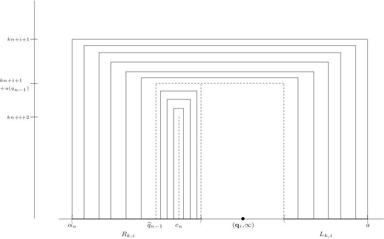
Figure 11. The crosscuts $\Gamma^{\prime}(y,k,i)$, in the case $k\geq 0$, drawn under the assumption that $q_{n-1}\in(c_{u},a]$, so that the interval $L_{k,i}$ is shorter than the interval $R_{k,i}$. In this figure the labels $\alpha_{u}$, ${\widehat{q}}_{n-1}$, $c_{u}$, and $a$ are abbreviations of $({\mathbf{t}}(\alpha_{u},k,i),\infty)$, $({\mathbf{t}}({\widehat{q}}_{n-1},k,i),\infty)$, $({\mathbf{t}}(c_{u},k,i),\infty)$, and $({\mathbf{t}}(a,k,i),\infty)$. The dotted lines represent limits of the crosscuts, which are not themselves of the form $\Gamma^{\prime}(y,k,i)$: see Remark 4.58.

Lemma 4.56.

For each $y\in(c_{u},a]\setminus\{\min(q_{n-1},{\widehat{q}}_{n-1})\}$, each $k\in{\mathbb{Z}}$, and each $0\leq i\leq n-1$, we have $\Gamma(y,k,i)={\widehat{H}}^{kn+i}(\Gamma(y,0,0))$.

Proof.

By Corollary 4.10 we have ${\widehat{H}}^{kn+i}(\Gamma(y,0,0))=\Psi(G^{kn+i}(\Gamma^{\prime}(y,0,0))$, where $G\colon\overline{D}\to\overline{D}$ is given (see Definition 4.1) by $G({\mathbf{y}},s)=({\widehat{B}}({\mathbf{y}}),\lambda(s))$. Now $G^{kn+i}(\Gamma^{\prime}(y,0,0))=\Gamma^{\prime}(y,k,i)$ by Remark 4.51 and the fact that $\lambda(s)=s+1$ for $s\geq 1$ and $\lambda(s)=2s$ for $s<1$. The result follows. ∎

The following is a key lemma for the remainder of the paper. It implies, in particular, that each crosscut $\Gamma(y,k,i)$ is contained in a stable set for ${\widehat{H}}$; and hence, by Lemma 4.56, that $\operatorname{diam}(\Gamma(y,k,i))\to 0$ as $k\to\infty$.

Lemma 4.57.

Let $y\in(c_{u},a]\setminus\{\min(q_{n-1},{\widehat{q}}_{n-1})\}$, $k\geq 0$, and $0\leq i\leq n-1$. Then every ${\mathbf{x}}\in\Gamma(y,k,i)$ has $x_{kn+i}=f(\tau(y))$.

Proof.

In view of Lemma 4.56, we need only show that every ${\mathbf{x}}\in\Gamma(y,0,0)$ has $x_{0}=f(\tau(y))$. Now

$$\Gamma(y,0,0) = \Psi\left(\xi^{\prime}([{\mathbf{t}}({\widehat{y}},0,0),{\mathbf{t}}(y,0,0)],\,\,1+u(y))\right)$$

$$= \Psi\left(\xi^{\prime}([\left<q_{0},{\widehat{y}},B^{-1}({\widehat{y}}),\ldots\right>,\left<q_{0},y,B^{-1}(y),\ldots\right>],\,\,1+u(y))\right).$$

1. Since ${\mathbf{t}}(y,0,0)_{1}=y$ and ${\mathbf{t}}(y,0,0)_{1+i}\not\in{{\accentset{\circ}{\gamma}}}$ for all $i\geq 1$, Lemma 4.20 gives that $\Psi({\mathbf{t}}(y,0,0),s)_{0}=f(\tau(y))$ for all $s\geq 1+u(y)$; similarly $\Psi({\mathbf{t}}({\widehat{y}},0,0),s)_{0}=f(\tau({\widehat{y}}))=f(\tau(y))$ for all $s\geq 1+u(y)$.

2. It remains to show that $\Psi({\mathbf{y}},1+u(y))_{0}=f(\tau(y))$ for all ${\mathbf{y}}\in[{\mathbf{t}}({\widehat{y}},0,0),{\mathbf{t}}(y,0,0)]$. Now in the case $y\in(\min(q_{n-1},{\widehat{q}}_{n-1}),a]$ we have, by Lemma 4.50,

   $$[{\mathbf{t}}({\widehat{y}},0,0),{\mathbf{t}}(y,0,0)]=\{{\mathbf{t}}(y^{\prime},0,0)\,:\,y^{\prime}\in[{\widehat{y}},y]\setminus\{q_{n-1}\}\}\,\,\,\,\cup\,\,\,\,\{{\mathbf{q}}_{0}\}\,\,\,\,\cup\,\,\,\,\bigcup_{k=1}^{\infty}\,\,(L_{k,0}\cup R_{k,0}),$$

   while in the case $y\in(c_{u},\min(q_{n-1},{\widehat{q}}_{n-1}))$ we have $[{\mathbf{t}}({\widehat{y}},0,0),{\mathbf{t}}(y,0,0)]=\{{\mathbf{t}}(y^{\prime},0,0)\,:\,y^{\prime}\in[{\widehat{y}},y]\}$.

   If $y^{\prime}\in[{\widehat{y}},y]$ with $y^{\prime}\not=q_{n-1}$ then

   $$\Psi({\mathbf{t}}(y^{\prime},0,0),1+u(y))_{0} = H(y^{\prime},\phi^{-1}(f(\tau(y))))$$

   $$= f(\tau(y))$$

   as required. Here the first equality uses (8) and that $(1+u(y))/2=\phi^{-1}(f(\tau(y)))$, while the second uses Lemma 4.5 and the fact that $u(y)\leq u(y^{\prime})$, since $y^{\prime}\in[{\widehat{y}},y]$.

   On the other hand, if we are in the case $y\in(\min(q_{n-1},{\widehat{q}}_{n-1}),a]$, and if ${\mathbf{y}}={\mathbf{q}}_{0}$ or ${\mathbf{y}}$ is in $L_{k,0}$ or $R_{k,0}$ for some $k\geq 1$, then $y_{1}=q_{n-1}$, and (8) and Lemma 4.5 give

   $$\Psi({\mathbf{y}},1+u(y))_{0}=H(q_{n-1},\phi^{-1}(f(\tau(y))))=f(\tau(y))$$

   as required, since $\phi^{-1}(f(\tau(y)))\leq u(q_{n-1})$.

∎

Remark 4.58.

There are two connected components of dotted lines on Figure 11, which are limits of the crosscuts $\Gamma^{\prime}(y,k,i)$. One is the arc $\{{\mathbf{t}}(c_{u},k,i)\}\times[kn+i+2,\infty]$, and the other is the union of the crosscut $\xi^{\prime}([{\mathbf{t}}({\widehat{q}}_{n-1},k,i),{\mathbf{t}}(a,k+1,i)],\,\,kn+i+1+u(q_{n-1}))$ and the crosscut $\xi^{\prime}([{\mathbf{t}}({\widehat{q}}_{n-1},k,i),{\mathbf{t}}(\alpha_{u},k+1,i)],\,kn+i+1+u(q_{n-1}))$, each interval in ${\widehat{S}}$ being the one which contains ${\mathbf{q}}_{i}$.

By the continuity of $\Psi$ on $\widetilde{D}$, every point $({\mathbf{y}},s)$ of the former has $\Psi({\mathbf{y}},s)_{kn+i}=f(\tau(c_{u}))=b$, and every point $({\mathbf{y}},s)$ of the latter has $\Psi({\mathbf{y}},s)_{kn+i}=f(\tau(q_{n-1}))=f^{n+1}(a)$.

Lemma 4.59.

1. Let $0\leq i\leq n-1$. For every sequence $(y^{(k)})$ in $(\min(q_{n-1},{\widehat{q}}_{n-1}),a]$, the sequence $(\Gamma^{\prime}(y^{(k)},k,i))_{k\geq 0}$ satisfies conditions (a) – (c) of Definition 4.22 (of a good chain of crosscuts for ${\mathbf{q}}_{i}$).

2. Let ${\mathbf{y}}\in{\widehat{S}}$. Then there is a good chain of crosscuts for ${\mathbf{y}}$.

Proof.

The sequence $(\Gamma^{\prime}(y^{(k)},k,i))_{k\geq 0}$ is a chain of crosscuts in $(\overline{D},{\widehat{S}}_{\infty})$ which satisfies condition (a) of Definition 4.22 by Lemma 4.52; it satisfies condition (b) by Lemma 4.50 (see Remark 4.55); and it satisfies condition (c) by Lemma 4.57, which gives that $\operatorname{diam}(\Gamma(y,k,i))\leq|b-a|/2^{kn+i}$.

For part (b) of the lemma, it suffices by Remark 4.23 (c) to find a good chain of crosscuts for each ${\mathbf{q}}_{i}$; that is, to show that we can choose the sequence $(y^{(k)})$ in such a way that $(\Gamma(y^{(k)},k,i))_{k\geq 0}$ does not converge to a point of ${\widehat{I}}$. The argument is similar to that used in the proof of Lemma 4.52.

Pick two distinct points $x,z\in[a,\min(\tau(q_{n-1}),\tau({\widehat{q}}_{n-1})))=[a,\theta)$, where $\theta=\min(f^{n}(a),\widehat{f^{n}(a)})$. By Lemma B.2, there are sequences $(x^{(k)})$ and $(z^{(k)})$ in $[a,\theta)$ with $f^{kn}(x^{(k)})=x$ and $f^{kn}(z^{(k)})=z$ for all sufficiently large $k$. Since $x^{(k)},z^{(k)}\in[a,\theta)$ we have $x_{u}^{(k)},z_{u}^{(k)}\in(\min(q_{n-1},{\widehat{q}}_{n-1}),a]$ for each $k$. Then, by Lemma 4.57, every ${\mathbf{x}}\in\Gamma(x_{u}^{(k)},k,i)$ has $x_{i+1}=x$, and every ${\mathbf{x}}\in\Gamma(z_{u}^{(k)},k,i)$ has $x_{i+1}=z$, provided that $k$ is sufficiently large.

Choosing $y^{(k)}=x_{u}^{(k)}$ when $k$ is even, and $y^{(k)}=z_{u}^{(k)}$ when $k$ is odd therefore gives a good chain of crosscuts. ∎

It follows from Theorem 4.28 and Lemma 4.31 that ${\mathcal{P}}\colon{\widehat{S}}\to{\mathbb{P}}$ is a homeomorphism, and that the prime end ${\mathcal{P}}({\mathbf{y}})$ is of the first kind for all ${\mathbf{y}}\not\in{\mathbf{Q}}$. It therefore only remains to calculate the principal sets and impressions of the prime ends ${\mathcal{P}}({\mathbf{q}}_{i})$. We will do this for ${\mathcal{P}}({\mathbf{q}}_{n-1})$: the analogous results for the other ${\mathcal{P}}({\mathbf{q}}_{i})$ follow on observing that ${\mathcal{P}}({\mathbf{q}}_{i})={\widehat{H}}^{i+1}({\mathcal{P}}({\mathbf{q}}_{n-1}))$ for each $i$ by Lemmas 4.56 and 4.59.

Lemma 4.60.

Let $f$ be of rational interior type, with $q(\kappa(f))=m/n$. Then ${\mathcal{I}}({\mathcal{P}}({\mathbf{q}}_{n-1}))={\widehat{I}}$.

Proof.

By Theorem 4.28 (b) and Lemma 4.59, ${\mathcal{P}}({\mathbf{q}}_{n-1})$ is defined by the chain $(\Gamma(a,k,n-1))_{k\geq 0}$, so it suffices to show that for every fixed ${\mathbf{x}}\in{\widehat{I}}$ and $k\geq 0$, we have ${\mathbf{x}}\in\overline{U(\Gamma(a,k,n-1))}$.

By Lemma B.1 there is some $N$ (which we take to be at least 3) with $f^{N}([a,\alpha])\supset f^{N}([a,c])=[a,b]$. For each $j$ with $jn\geq N$, we can therefore choose $z^{(j)}\in[a,\alpha]\setminus\{\tau(q_{n-1})\}$ with $f^{N}(z^{(j)})=x_{jn-N}$. (If $x_{jn-N}=f^{N}(\tau(q_{n-1}))$ then we also have $x_{jn-N}=f^{N}(\tau({\widehat{q}}_{n-1}))$, and either $\tau({\widehat{q}}_{n-1})\not=\tau(q_{n-1})$ or $x_{jn-N}=f^{N}(c)$. In the latter case we have $x_{jn-N}=f^{N-2}(a)=f^{N-2}(\alpha)$, and since $\alpha$ has two $f$-preimages there is some $z^{(j)}\not=c$ with $f^{N}(z^{(j)})=x_{jn-N}$.)

For each such $j$, let

$${\mathbf{y}}^{(j)}={\mathbf{t}}(z_{u}^{(j)},j-1,n-1)=\left<(q_{n-1},\ldots,q_{0})^{j},z_{u}^{(j)},B^{-1}(z_{u}^{(j)}),\ldots\right>,$$

which is landing of level $jn$. By (17) we have $\omega({\mathbf{y}}^{(j)})_{jn-N}=f^{N}(z^{(j)})=x_{jn-N}$, so that $\omega({\mathbf{y}}^{(j)})\to{\mathbf{x}}$ as $j\to\infty$. Since $({\mathbf{y}}^{(j)},\infty)\in\overline{U(\Gamma^{\prime}(a,k,n-1)}$ for all $j>k$, we have $\omega({\mathbf{y}}^{(j)})\in\overline{U(\Gamma(a,k,n-1))}$ for all $j>k$, and hence ${\mathbf{x}}\in\overline{U(\Gamma(a,k,n-1))}$ as required. ∎

Lemma 4.61.

Let $f$ be of rational interior type, with $q(\kappa(f))=q=m/n$. If $\kappa(f)\succ w_{q}0\left(w_{q}1\right)^{\infty}$ then $\Pi({\mathcal{P}}({\mathbf{q}}_{n-1}))={\widehat{I}}$.

Proof.

Let ${\mathbf{x}}\in{\widehat{I}}$. We show that ${\mathbf{x}}\in\Pi({\mathcal{P}}({\mathbf{q}}_{n-1}))$ by exhibiting a chain of crosscuts defining ${\mathcal{P}}({\mathbf{q}}_{n-1})$ which converges to ${\mathbf{x}}$.

By Lemma B.2 (b), there is some $N\in{\mathbb{N}}$ with $f^{N}([a,\theta))=[a,b]$, where $\theta=\min(f^{n}(a),\widehat{f^{n}(a)})$. For each $k$ with $kn\geq N$, pick $z^{(k)}\in[a,\theta)$ with $f^{N}(z^{(k)})=x_{kn-N}$. Since $z^{(k)}\in[a,\theta)$ we have $z^{(k)}_{u}\in(\min(q_{n-1},{\widehat{q}}_{n-1}),a]$ for each $k$. Therefore, by Lemma 4.59 (a), ${\mathcal{P}}({\mathbf{q}}_{n-1})$ is defined by the chain $(\Gamma(z_{u}^{(k)},k-1,n-1))_{k\geq N/n}$.

By Lemma 4.57, every ${\mathbf{v}}\in\Gamma(z^{(k)}_{u},k-1,n-1)$ has $v_{kn-1}=f(z^{(k)})$, and hence $v_{kn-N}=x_{kn-N}$. Therefore $\Gamma(z^{(k)}_{u},k-1,n-1)\to{\mathbf{x}}$ as $k\to\infty$ as required. ∎

Lemma 4.62.

Let $f$ be of rational interior type, with $q(\kappa(f))=q=m/n$. If $\kappa(f)\preceq w_{q}0\left(w_{q}1\right)^{\infty}$ then $\Pi({\mathcal{P}}({\mathbf{q}}_{n-1}))=\{{\mathbf{x}}\in{\widehat{I}}\,:\,x_{\ell n}\in[a,f^{n}(a)]\text{ for all }\ell\geq 0\}$.

Proof.

This is a consequence of Lemma B.2 (a), which states that $f^{n}([a,f^{n}(a)))=[a,f^{n}(a)]$ whenever $\left(w_{q}0\right)^{\infty}\prec\kappa(f)\preceq w_{q}0\left(w_{q}1\right)^{\infty}$.

Write $X=\{{\mathbf{x}}\in{\widehat{I}}\,:\,x_{\ell n}\in[a,f^{n}(a)]\text{ for all }\ell\geq 0\}$. To show that $X\subset\Pi({\mathcal{P}}({\mathbf{q}}_{n-1}))$, we exhibit, for each ${\mathbf{x}}\in X$, a chain of crosscuts defining ${\mathcal{P}}({\mathbf{q}}_{n-1})$ which converges to ${\mathbf{x}}$. By Lemma B.2 (a), $f^{n}(a)_{u}=\min(q_{n-1},{\widehat{q}}_{n-1})$, and for each $k\geq 0$ there is some $z^{(k)}\in[a,f^{n}(a))$ with $f^{n}(z^{(k)})=x_{kn}$. By Lemma 4.57, every ${\mathbf{v}}\in\Gamma(z_{u}^{(k)},k,n-1)$ has $v_{(k+1)n-1}=f(z^{(k)})$, and hence $v_{kn}=x_{kn}$. Therefore $(\Gamma(z^{(k)},k,n-1))_{k\geq 0}$ is a chain of crosscuts defining ${\mathcal{P}}({\mathbf{q}}_{n-1})$ which converges to ${\mathbf{x}}$.

To show that $\Pi({\mathcal{P}}({\mathbf{q}}_{n-1}))\subset X$, it is enough, by Theorem 4.28 (c), to show that $\operatorname{Rem}(R_{{\mathbf{q}}_{n-1}})\subset X$. To do this, we fix $\ell\geq 0$ and show that $R_{{\mathbf{q}}_{n-1}}(s)_{\ell n}\in[a,f^{n}(a)]$ for all $s\geq\ell n+1$.

We therefore fix $s\geq\ell n+1$, and write $P(s)=(t,v)$. Recalling that ${\mathbf{q}}_{n-1}=\left<(q_{n-1},\ldots,q_{0})^{\infty}\right>$, using (8), and abbreviating $R_{{\mathbf{q}}_{n-1}}$ to $R$:

1. If $t=rn$ for some $r\geq\ell+1$ then

   $$R(s)_{rn-1}=H(q_{n-1},v)\in[f(a),f(\tau(q_{n-1}))]=[f(a),f^{n+1}(a)].$$

   Since $f^{n-1}([f(a),f^{n+1}(a)])=[a,f^{n}(a)]$ by Lemma B.2 (a), we have $R(s)_{(r-1)n}\in[a,f^{n}(a)]$, and hence $R(s)_{\ell n}\in[a,f^{n}(a)]$ as required.

2. If $t=rn+i$ for some $r\geq\ell$ and $1\leq i\leq n-1$ then

   $$R(s)_{rn+i-1}=R(s)_{t-1}=H(q_{n-1-i},v)=\tau(B(q_{n-1-i}))=\tau(q_{n-i})=f^{n-i+1}(a),$$

   since $q_{n-1-i}\not\in{{\accentset{\circ}{\gamma}}}$. Therefore $R(s)_{rn}=f^{n}(a)$, and hence $R(s)_{\ell n}\in[a,f^{n}(a)]$ as required.

∎

Remark 4.63.

Since ${\mathcal{P}}({\mathbf{q}}_{i})={\widehat{H}}^{i+1}({\mathcal{P}}({\mathbf{q}}_{n-1}))$ for $0\leq i<n-1$, it follows that, whenever we have $\left(w_{q}0\right)^{\infty}\prec\kappa(f)\preceq w_{q}0\left(w_{q}1\right)^{\infty}$,

$$\Pi({\mathcal{P}}({\mathbf{q}}_{i}))=\{{\mathbf{x}}\in{\widehat{I}}\,:\,x_{\ell n+i+1}\in[a,f^{n}(a)]\text{ for all }\ell\geq 0\}.$$

These principal sets are therefore homeomorphic to the inverse limit $\varprojlim([a,f^{n}(a)],f^{n})$ of the renormalized map.

The following theorem provides a summary of what we have proved in the rational interior case.

Theorem 4.64 (Prime ends in the rational interior case).

Let $f$ be a unimodal map satisfying the conditions of Convention 2.8, and suppose that $q(\kappa(f))=m/n\in(0,1/2)$ is rational, and that $\kappa(f)\not\in\{\operatorname{lhe}(m/n),(w_{m/n}0)^{\infty},\operatorname{rhe}(m/n)\}$. Then

1. All except $n$ of the prime ends of $({\widehat{T}},{\widehat{I}})$ are of the first kind;

2. If $\kappa(f)\preceq w_{m/n}0\left(w_{m/n}1\right)^{\infty}$, then the $n$ remaining prime ends are of the fourth kind, with principal set $\varprojlim([a,f^{n}(a)],f^{n})$ and impression ${\widehat{I}}$;

3. If $\kappa(f)\succ w_{m/n}0\left(w_{m/n}1\right)^{\infty}$, then the $n$ remaining prime ends are of the third kind, with principal set and impression ${\widehat{I}}$; and

4. The prime end rotation number is $m/n$. ∎

Remark 4.65.

By Theorem 4.28 (d), the set of accessible points of ${\widehat{I}}$ is precisely $\{\omega({\mathbf{y}})\,:\,{\mathbf{y}}\in{\widehat{S}}\setminus{\mathbf{Q}}\}$. This set is partitioned into $n$ immersed copies of the line.

4.7. The rational endpoint case

We finish by considering the rational endpoint case, where $\mu=\kappa(f)$ has rational height $q=q(\mu)\in(0,1/2)$ and $\mu=\operatorname{lhe}(q)$, $\mu=\operatorname{rhe}(q)$, or $\mu=\left(w_{q}0\right)^{\infty}$; or where $q=0$. The following theorem summarizes this case.

Theorem 4.66 (Prime ends in the rational endpoint case).

Let $f$ be a unimodal map satisfying the conditions of Convention 2.8, and suppose that $q(\kappa(f))=m/n\in[0,1/2)$ is rational, and that $\kappa(f)\in\{\operatorname{lhe}(m/n),(w_{m/n}0)^{\infty},\operatorname{rhe}(m/n)\}$. Then

1. All except $n$ of the prime ends of $({\widehat{T}},{\widehat{I}})$ are of the first kind;

2. The $n$ remaining prime ends are of the second kind, with impression ${\widehat{I}}$; and

3. The prime end rotation number is $m/n$.

The arguments in the four cases where $f$ is of early endpoint, normal endpoint, quadratic-like strict left endpoint, or late endpoint type are different, and we consider each of them briefly in turn, pointing out how they differ from similar arguments in the rational interior and irrational cases, and leaving the reader to fill in some details.

4.7.1. The normal endpoint case

In this case either $\mu=\operatorname{lhe}(m/n)$ and $B^{n}(a)=a$, or $\mu=\operatorname{rhe}(m/n)$ and $B^{n}(a)=\alpha_{u}$; and the orbit of $B(a)$ is the only periodic orbit of $B$. We will consider the case where $\mu=\operatorname{lhe}(m/n)$: the other case can be treated in exactly the same way. Minor modifications are needed in the particular case $m/n=0$ (i.e. when $\mu=10^{\infty}$): we will assume that $m/n>0$.

The analysis starts in the same way as the rational interior case. We write $q_{i}=B^{i+1}(a)$ for $0\leq i\leq n-1$, so that $Q=\{q_{0},q_{1},\ldots,q_{n-1}\}$ is a period $n$ orbit of $B$, with $q_{n-1}=a\in\gamma$. Threads ${\mathbf{q}}_{i}$ and ${\mathbf{t}}(y,k,i)$ in ${\widehat{S}}$, and the periodic orbit ${\mathbf{Q}}$ of ${\widehat{B}}$, are introduced exactly as in Definitions 4.48.

Intervals $R_{k,i}$ can then be constructed as in Definitions 4.49. However, since $q_{n-1}=a$, the intervals $L_{k,i}$ of the rational interior case are empty. This means that the intervals $R_{k,i}$ converge to ${\mathbf{q}}_{i}$ as $k\to\infty$, and to ${\mathbf{q}}_{j}$ as $k\to-\infty$, where $j=i-m^{-1}\bmod{n}$ (Figure 12).

Figure 12. The intervals $R_{k,i}$ in the normal endpoint case when $B^{n}(a)=a$.

Since the threads ${\mathbf{q}}_{i}$ do not contain any entries from ${{\accentset{\circ}{\gamma}}}$, the points of ${\mathbf{Q}}$ are landing of level 0, and hence ${\mathcal{L}}={\widehat{S}}$. On the other hand, ${\mathcal{R}}={\widehat{S}}\setminus{\mathbf{Q}}$, since the interior points of $R_{k,i}$ are not landing of any level less than $kn+i+1$.

The construction of good chains of crosscuts for each ${\mathbf{q}}_{i}$ is reminiscent of the irrational gap endpoint case.

Lemma 4.67.

Let $0\leq i\leq n-1$. Write $V=\bigcup_{k<0}R_{k,i+m^{-1}\bmod{n}}$, and let $\left({\mathbf{y}}^{(k)}\right)$ be any sequence in $V$ which converges strictly monotonically to ${\mathbf{q}}_{i}$. For each $k\geq 1$, let ${\mathbf{J}}_{k}$ be the interval in ${\widehat{S}}$ with endpoints ${\mathbf{y}}^{(k)}$ and ${\mathbf{t}}(\alpha_{u},k,i)$ which contains ${\mathbf{q}}_{i}$. Let

$$\xi^{\prime}_{k}=\xi^{\prime}({\mathbf{J}}_{k},\,nk+i).$$

Then $(\xi^{\prime}_{k})$ is a good chain of crosscuts for ${\mathbf{q}}_{i}$.

Proof.

Conditions (a) and (b) of Definition 4.22 are immediate, and condition (d) is vacuous. It is therefore only necessary to show that $\operatorname{diam}(\xi_{k})\to 0$ as $k\to\infty$, where $\xi_{k}=\Psi(\xi^{\prime}_{k})$.

We have $\operatorname{diam}(\xi_{k}\cap\Psi\left(\overline{V}\times[0,\infty]\right))\to 0$, since $\Psi$ is continuous on $\overline{V}\times[0,\infty]$ by Lemma 4.17. To show that the diameters of the remaining parts of $\xi_{k}$ go to zero, we will show that every ${\mathbf{x}}$ belonging to the arc $\Psi(\{{\mathbf{t}}(\alpha_{u},k,i)\}\times[nk+i,\infty])$ or to the arc $\Psi(({\mathbf{J}}_{k}\setminus V)\times\{nk+i\})$ has $x_{nk+i-1}=\tau(q_{1})$.

For the former, we have $\Psi({\mathbf{t}}(\alpha_{u},k,i),s)_{nk+i-1}=\tau({\mathbf{t}}(\alpha_{u},k,i)_{nk+i-1})=\tau(q_{1})$ for all $s\geq nk+i$ by Lemma 4.13, since ${\mathbf{t}}(\alpha_{u},k,i)$ is landing of level 0 (and hence of level $nk+i-1$).

For the latter, observe that if ${\mathbf{y}}\in{\mathbf{J}}_{k}\setminus V$ then $y=\left<q_{i},\ldots,q_{0},(q_{n-1},\ldots,q_{0})^{k},\ldots\right>$ and so $y_{nk+i}=q_{0}$. Therefore, by (8), $\Psi({\mathbf{y}},nk+i)_{nk+i-1}=H(q_{0},1/2)=\tau(q_{1})$ as required. ∎

It follows from Theorem 4.28 and Lemma 4.31 that ${\mathcal{P}}\colon{\widehat{S}}\to{\mathbb{P}}$ is a homeomorphism; that the prime end ${\mathcal{P}}({\mathbf{y}})$ is of the first kind for all ${\mathbf{y}}\not\in{\mathbf{Q}}$; and that $\Pi({\mathcal{P}}({\mathbf{y}}))=\{\omega({\mathbf{y}})\}$ is a point for ${\mathbf{y}}\in{\mathbf{Q}}$. It therefore only remains to calculate the impressions of the prime ends ${\mathcal{P}}({\mathbf{q}}_{i})$. The proof of the following result works in exactly the same way as that of Lemma 4.60, using the chain of crosscuts from Lemma 4.67 in place of the chain $(\Gamma(a,k,n-1))_{k\geq 0}$.

Lemma 4.68.

Let $f$ be of normal endpoint type, with $q(\kappa(f))=m/n$. Then ${\mathcal{I}}({\mathcal{P}}({\mathbf{q}}_{n-1}))={\widehat{I}}$. ∎

4.7.2. The quadratic-like strict left endpoint case

In this case $\mu=\operatorname{lhe}(m/n)$ and $B^{n}(a)=a$, but $B$ has a second period $n$ orbit $P$ in addition to the orbit of $B(a)$. As in the rational interior case, we write $q_{i}=B^{i+1}(a)$ for $0\leq i\leq n-1$, $p_{0}$ for the point of $P$ between $q_{0}$ and $q_{m^{-1}\bmod{n}}$, and $p_{i}=B^{i}(p_{0})$ for $1\leq i\leq n-1$. Threads ${\mathbf{q}}_{i}$, ${\mathbf{p}}_{i}$, and ${\mathbf{t}}(y,k,i)$ in ${\widehat{S}}$, and the periodic orbits ${\mathbf{Q}}$ and ${\mathbf{P}}$ of ${\widehat{B}}$ are introduced exactly as in Definitions 4.48. However, since the $B$-orbits of points in each interval $(q_{i},p_{i}]$ are disjoint from $\gamma$, there are threads

$${\mathbf{t}}(y)=\left<y,B^{-1}(y),B^{-2}(y),\ldots\right>\qquad\text{ for }y\in\bigcup_{i=0}^{n-1}(q_{i},p_{i}]$$

in ${\widehat{S}}$ (with ${\mathbf{t}}(p_{i})={\mathbf{p}}_{i}$). We write $I_{i}=\{{\mathbf{t}}(y)\,:\,y\in(q_{i},p_{i}]\}$ for $0\leq i\leq n-1$, half-open intervals in ${\widehat{S}}$ with ${\widehat{B}}(I_{i})=I_{i+1\bmod{n}}$. Defining half-open intervals $R_{k,i}$ as in Definitions 4.49, the intervals are arranged around ${\widehat{S}}$ as depicted in Figure 13 (where $j=i-m^{-1}\bmod{n}$).

Figure 13. Intervals around ${\widehat{S}}$ in the quadratic-like left strict endpoint case.

The remainder of the analysis proceeds exactly as in the normal endpoint case, except that in the statement of Lemma 4.67 we take $V=I_{i}$ rather than $V=\bigcup_{k<0}R_{k,i+m^{-1}\bmod{n}}$.

4.7.3. The late endpoint case

Here $q=m/n>0$ and $\mu=\left(w_{q}0\right)^{\infty}$. In this case $q_{n-1}=B^{n}(a)\in{{\accentset{\circ}{\gamma}}}$ by Theorem 4.33 (b)(ii), and the treatment is identical to that of the rational interior case up until Lemma 4.52. Here, because Lemma B.2 doesn’t apply when $\kappa(f)=\left(w_{q}0\right)^{\infty}$, the proof that ${\mathcal{L}}={\widehat{S}}\setminus{\mathbf{Q}}$ breaks down. Instead we have:

Lemma 4.69.

Let $f$ be of late endpoint type. Then ${\mathcal{L}}={\widehat{S}}$.

Proof.

The points $a$ and $f^{n}(a)$ are distinct, but both have itinerary $\sigma(\left(w_{q}0\right)^{\infty})$. Since $w_{q}0$ is a word of length $n$ with an odd number of $1$s, $f^{n}|_{[a,f^{n}(a)]}$ is decreasing, with $a<f^{2n}(a)<f^{n}(a)$. There is therefore a unique fixed point $p$ of $f^{n}$ in $[a,f^{n}(a)]$. Now the increasing map $f^{2n}\colon[a,f^{n}(a)]\to[a,f^{n}(a)]$ also has $p$ as its unique fixed point (any other fixed points would be period 2 points of $f^{n}$ and so would come in pairs, contradicting Convention 2.8 (c)), so that $f^{kn}(x)\to p$ as $k\to\infty$ for every $x\in[a,f^{n}(a)]$.

Since every point of ${\widehat{S}}\setminus{\mathbf{Q}}$ is landing of some level, it is only necessary to prove that the rays $R_{{\mathbf{q}}_{i}}$ land. It is enough to show this for $i=n-1$ since $R_{{\mathbf{q}}_{i}}={\widehat{H}}^{i+1}\circ R_{{\mathbf{q}}_{n-1}}$ for $0\leq i\leq n-2$.

Fix $r\geq 0$ and let $s\geq r+1$. Write $P(s)=(t,v)$ and $t=kn+i$ with $0\leq i\leq n-1$: then (8) gives $\Psi({\mathbf{q}}_{n-1},s)_{r}=f^{t-1-r}(H(q_{n-1-i},v))$. If $i\not=0$ then $H(q_{n-1-i},v)=\tau(q_{n-i})=f^{n-i+1}(a)$, so that $\Psi({\mathbf{q}}_{n-1},s)_{r}=f^{(k+1)n-r}(a)$. On the other hand, if $i=0$ then $H(q_{n-1-i},v)\in[f(a),f^{n+1}(a)]$ by Definition 3.2, so that $\Psi({\mathbf{q}}_{n-1},s)_{r}=f^{kn-r}(x)$ for some $x\in[a,f^{n}(a)]$.

Therefore $\Psi({\mathbf{q}}_{n-1},s)_{r}\to f^{n-r}(p)$ as $s\to\infty$. It follows that

$$\Psi({\mathbf{q}}_{n-1},s)\to\omega({\mathbf{q}}_{n-1})=\left<(p,f^{n-1}(p),\ldots,f(p))^{\infty}\right>\text{ as }s\to\infty,$$

so that ${\mathbf{q}}_{n-1}\in{\mathcal{L}}$ as required. ∎

Remark 4.70.

Thus, in the late endpoint case, the points of ${\mathbf{Q}}$ are landing, despite not being landing of any level. This is the only case in which ${\mathcal{L}}\not=\bigcup_{N\geq 0}{\mathcal{L}}_{N}$.

Since the interior points of $R_{k,i}$ are not landing of any level less than $kn+i+1$, the locally uniformly landing set is given by ${\mathcal{R}}={\widehat{S}}\setminus{\mathbf{Q}}$. The proof of Lemma 4.59 (a) goes through without change to show that $(\Gamma^{\prime}(a,k,i))_{k\geq 0}$ is a good chain of crosscuts for ${\mathbf{q}}_{i}$ (observing that condition (d) of Definition 4.22 is vacuous); and the proof of Lemma 4.60 likewise carries over to show that ${\mathcal{I}}({\mathcal{P}}({\mathbf{q}}_{n-1}))={\widehat{I}}$.

4.7.4. The early endpoint case

In this case $q=m/n>0$ and $\mu=\operatorname{lhe}(m/n)$, but $f^{n}(a)\not=a$. According to Theorem 4.33 (c)(ii), the orbit ${\mathcal{O}}=\{B^{r}(a)\,:\,r\geq 1\}$ is disjoint from $\gamma$, and is attracted to a period $n$ orbit $Q\subset S\setminus\gamma$ of $B$: in particular, $B^{-r}(y)$ is defined for all $r\geq 0$ provided that $y\not\in{\mathcal{O}}$. There are two possibilities: either $Q$ is semi-stable and is the only periodic orbit of $B$, in which case the backwards orbit $\{B^{-r}(\gamma)\,:\,r\geq 0\}$ of $\gamma$ is attracted to $Q$; or $Q$ is stable, and there is a repelling period $n$ orbit $P\subset S\setminus\gamma$ of $B$, which attracts the backwards orbit of $\gamma$.

The analysis initially follows that of the irrational case. Elements of ${\widehat{S}}$ can be written either as ${\mathbf{t}}(y,r)$, with $y\in\gamma$ and $r\in{\mathbb{Z}}$; or as ${\mathbf{t}}(y)$ with $y\in S\setminus\bigcup_{r\in{\mathbb{Z}}}B^{-r}(\gamma)$, these threads being defined exactly as in Definitions 4.37. It follows, as in the proof of Lemma 4.38, that ${\mathcal{L}}={\widehat{S}}$. “Gaps” $G_{r}=\{{\mathbf{t}}(y,r)\,:\,y\in\gamma\}$ can be defined as in Definition 4.39.

The difference with the irrational case is that the gaps $G_{r}$ converge as $r\to\infty$ to the periodic orbit ${\mathbf{Q}}$ of ${\widehat{B}}$ corresponding to $Q$; and they converge as $r\to-\infty$ either to ${\mathbf{Q}}$ from the other side (in the case where $Q$ is the unique periodic orbit of $B$), or to the periodic orbit ${\mathbf{P}}$ of ${\widehat{B}}$ corresponding to $P$. Since $G_{r}$ is uniformly landing of level $\max(r,0)$, we have in either case that ${\mathcal{R}}={\widehat{S}}\setminus{\mathbf{Q}}$.

The construction of a good chain of crosscuts for each point ${\mathbf{q}}$ of ${\mathbf{Q}}$ can be carried out in exactly the same way as in the irrational case (Lemma 4.44); and the proof that ${\mathcal{I}}({\mathcal{P}}({\mathbf{q}}))={\widehat{I}}$ for each such ${\mathbf{q}}$ is identical to the proof of Lemma 4.45.

Remark 4.71.

By Theorem 4.28 (d), the set of accessible points of ${\widehat{I}}$ is precisely $\{\omega({\mathbf{y}})\,:\,{\mathbf{y}}\in{\widehat{S}}\}$. Since the landing function $\omega$ is continuous from one side, but not from the other, at the points of ${\mathbf{Q}}$, the set of accessible points is partitioned into $n$ immersed copies of $[0,\infty)$.

5. Semi-conjugacy to sphere homeomorphisms

In this section we will prove (Theorem 5.19) that if $\{f_{t}\}$ is a continuously varying family of unimodal maps, then there is a corresponding family $\{\chi_{t}\colon S^{2}\to S^{2}\}$ of sphere homeomorphisms such that each $\chi_{t}$ is a factor of ${\widehat{f}}_{t}\colon{\widehat{I}}_{t}\to{\widehat{I}}_{t}$ by a semi-conjugacy with mild point preimages. In order to simplify the exposition, we start by treating the case of a single unimodal map $f$ (Theorem 5.15).

We will also show (Theorem 5.31) that if $\{f_{t}\}$ is a family of tent maps, then $\chi_{t}$ is a generalized pseudo-Anosov map for those values of $t$ for which $f_{t}$ is post-critically finite (and is pseudo-Anosov when $f_{t}$ is of NBT type). Therefore, in the tent map case, $\{\chi_{t}\}$ is a completion of the family of generalized pseudo-Anosovs constructed in [21].

In order to construct the semi-conjugacy, we will define a non-separating monotone upper semi-continuous decomposition ${\mathcal{G}}$ of ${\widehat{T}}$, whose elements are permuted by ${\widehat{H}}$, and each of which intersects ${\widehat{I}}$. By Moore’s theorem [32], the quotient space $\Sigma={\widehat{T}}/{\mathcal{G}}$ is again a sphere, and $F={\widehat{H}}/{\mathcal{G}}\colon\Sigma\to\Sigma$ is a homeomorphism. Since each of the decomposition elements intersects ${\widehat{I}}$, the natural projection ${\widehat{T}}\to\Sigma$ induces a surjection ${\widehat{I}}\to\Sigma$, which semi-conjugates ${\widehat{f}}={\widehat{H}}|_{{\widehat{I}}}$ to $F$.

To define the decomposition ${\mathcal{G}}$, we first introduce the strongly stable equivalence relation on ${D^{{\scriptstyle\dagger}}}$ (Definition 5.1). (Recall that ${D^{{\scriptstyle\dagger}}}=D\cup{\mathcal{L}}_{\infty}\subset\overline{D}$ is the maximal domain of $\Psi$.) The idea is that a strongly stable component of ${\widehat{T}}$ is a maximal connected subset $X$ of ${\widehat{T}}$ with the property that, for all ${\mathbf{x}}^{(1)},{\mathbf{x}}^{(2)}\in X$, there is some $N\geq 0$ with ${\widehat{H}}^{N}({\mathbf{x}}^{(1)})_{0}={\widehat{H}}^{N}({\mathbf{x}}^{(2)})_{0}$. A consequence of this is that $d({\widehat{H}}^{i}({\mathbf{x}}^{(1)}),{\widehat{H}}^{i}({\mathbf{x}}^{(2)}))\to 0$ as $i\to\infty$, so that strongly stable sets are stable: the converse is not true in general, since the unimodal map $f$ may itself have non-trivial connected stable sets. Now such a subset $X$ may intersect ${\widehat{I}}$ (and hence leave the image of $\Psi$) many times. A strongly stable component of ${D^{{\scriptstyle\dagger}}}$ is a component of the preimage $\Psi^{-1}(X)$. Our decomposition will be based on these components.

In Lemmas 5.3, 5.5, 5.6, 5.7, and 5.8 we describe the structure of the strongly stable equivalence classes for each of the types of unimodal map of Definition 2.25. We then use these to construct a decomposition ${\mathcal{G}}^{\prime}$ of $\overline{D}$: one of the decomposition elements is the union of $\partial^{\prime}$ and all of the strongly stable equivalence classes whose closure contains $\partial^{\prime}$, while all of the other decomposition elements are single strongly stable equivalence classes or single points not in ${D^{{\scriptstyle\dagger}}}$. The decomposition ${\mathcal{G}}$ is obtained by carrying over ${\mathcal{G}}^{\prime}$ with $\Psi$, and adding single inaccessible points of ${\widehat{I}}$ (which, by Theorem 4.28 (d), are precisely the points which are not in the image of $\Psi$).

Definition 5.1 (Strongly stable, strongly stable component).

A subset $Y$ of ${D^{{\scriptstyle\dagger}}}$ is said to be strongly stable if, for all $\eta_{1},\eta_{2}\in Y$, there is some $N\geq 0$ such that ${\widehat{H}}^{N}(\Psi(\eta_{1}))_{0}={\widehat{H}}^{N}(\Psi(\eta_{2}))_{0}$.

The strongly stable component of $\eta\in{D^{{\scriptstyle\dagger}}}$ is the largest connected strongly stable set which contains $\eta$ (i.e. the union of all such connected strongly stable sets).

Remarks 5.2.

1. Since $G$ and ${\widehat{H}}$ are topologically conjugate (Corollary 4.10), the homeomorphism $G\colon{D^{{\scriptstyle\dagger}}}\to{D^{{\scriptstyle\dagger}}}$ permutes the strongly stable components.

2. $\{\partial^{\prime}\}$ is a strongly stable component, since if $({\mathbf{y}},s)\not=\partial^{\prime}$ then ${\widehat{H}}^{N}(\Psi(\partial^{\prime}))_{0}=\partial\not={\widehat{H}}^{N}(\Psi({\mathbf{y}},s))_{0}$ for all $N\geq 0$.

5.1. Strongly stable components in the irrational and the rational early endpoint cases

Recall from Section 4.5 that if $f$ is of irrational type then ${\mathcal{L}}={\widehat{S}}$, so that ${D^{{\scriptstyle\dagger}}}=\overline{D}$; that ${\widehat{B}}\colon{\widehat{S}}\to{\widehat{S}}$ is a Denjoy counterexample, having an orbit $\{G_{r}\,:\,r\in{\mathbb{Z}}\}$ of wandering intervals; and that the complement of the union of the interiors of these intervals is a Cantor set $\Lambda$, which is the set of points which are not locally uniformly landing.

If $f$ is of rational early endpoint type (Section 4.7.4) then the description is the same as in the irrational case, except that the orbit of the intervals $G_{r}$ converges as $r\to\infty$ and as $r\to-\infty$ to periodic orbits ${\mathbf{Q}}$ and ${\mathbf{P}}$ of ${\widehat{B}}$, and ${\mathcal{R}}={\widehat{S}}\setminus{\mathbf{Q}}$. If ${\mathbf{Q}}$ and ${\mathbf{P}}$ are distinct, then the former is stable and the latter is unstable; while if ${\mathbf{P}}={\mathbf{Q}}$, then this is a semi-stable orbit, which is the limit on one side of the intervals $G_{r}$ as $r\to\infty$, and on the other side of the intervals $G_{r}$ as $r\to-\infty$.

The following lemma is illustrated in the irrational case by Figure 14. The picture in the early endpoint case is discussed in Remark 5.4.

Lemma 5.3.

Let $f$ be of irrational type or of rational early endpoint type. Then the strongly stable components of ${D^{{\scriptstyle\dagger}}}$ are $\{\partial^{\prime}\}$ and:

1. for each ${\mathbf{y}}\in{\widehat{S}}\setminus\bigcup_{r\in{\mathbb{Z}}}G_{r}$, the line $L_{{\mathbf{y}}}=\{{\mathbf{y}}\}\times(0,\infty]$;

2. for each $r\in{\mathbb{Z}}$:

   1. the arc $A_{r}=\{{\mathbf{t}}(c_{u},r)\}\times[s_{r},\infty]$; where $s_{r}=\lambda^{r}(1)$, i.e.

      $$s_{r}=\begin{cases}r+1&\text{ if }r\geq 1,\\ 1/2^{|r|}&\text{ if }r\leq 0.\end{cases}$$

   2. for each $y\in(c_{u},a)$, the crosscut $C_{r,y}=\xi^{\prime}({\mathbf{J}}_{r,y},t_{r,y})$; where ${\mathbf{J}}_{r,y}\subset G_{r}$ has endpoints ${\mathbf{t}}(y,r)$ and ${\mathbf{t}}({\widehat{y}},r)$, and $t_{r,y}=\lambda^{r}((1+u(y))/2)$, i.e.

      $$t_{r,y}=\begin{cases}r+u(y)&\text{ if }r\geq 1,\\ (1+u(y))/2^{|r|+1}&\text{ if }r\leq 0.\end{cases}$$

   3. the union $D_{r}$ of the arcs ${\mathbf{t}}(a,r)\times[u_{r},\infty]$ and ${\mathbf{t}}(\alpha_{u},r)\times[u_{r},\infty]$, and the set $G_{r}\times(0,u_{r}]$; where $u_{r}=s_{r-1}=\lambda^{r}(1/2)$, i.e.

      $$u_{r}=\begin{cases}r&\text{ if }r\geq 1,\\ 1/2^{|r|+1}&\text{ if }r\leq 0.\end{cases}$$

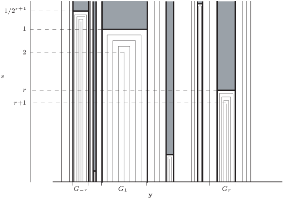
Figure 14. Strongly stable components in the irrational case. The types of components are: (a) vertical lines $L_{\mathbf{y}}$ above the buried points ${\mathbf{y}}$ of the Cantor set $\Lambda$; (b) packets of crosscuts $C_{r,y}$ above each gap $G_{r}$, together with the “central” arc $A_{r}$ which only intersects ${\widehat{S}}_{\infty}$ at a single point; and (c) for each gap $G_{r}$, the set $D_{r}$ consisting of the outermost crosscut above $G_{r}$ together with the rectangle above this crosscut extending up to (but not including) $s=0$. Each set $D_{r}$ is shown as the union of a shaded rectangle and the bold arcs which intersect it.

Proof.

We first show that each of the sets listed is strongly stable.

1. Let ${\mathbf{y}}\in{\widehat{S}}\setminus\bigcup_{r\in{\mathbb{Z}}}G_{r}$, so that ${\mathbf{y}}=\left<y,B^{-1}(y),B^{-2}(y),\ldots\right>$ for some $y$ whose orbit under $B$ is disjoint from $\gamma$. Since ${\mathbf{y}}$ is landing of level 0, Lemma 4.13 gives $\Psi({\mathbf{y}},s)_{0}=\tau(y)$ for all $s\geq 1$. Applying $G$ repeatedly (or arguing directly using that $\Psi({\mathbf{y}},s)=\left<(y,s),(B^{-1}(y),s/2),\ldots\right>$ for $s\in[0,1)$) gives that, for each $m\geq 1$, ${\widehat{H}}^{m}(\Psi({\mathbf{y}},s))_{0}=f^{m}(\tau(y))$ for all $s\in[1/2^{m},\infty]$. Therefore $L_{{\mathbf{y}}}$ is strongly stable.

2. $G(A_{r})=A_{r+1}$, $G(C_{r,y})=C_{r+1,y}$, and $G(D_{r})=D_{r+1}$ for all $r\in{\mathbb{Z}}$ and $y\in(c_{u},a)$. Since $G$ permutes strongly stable components, it suffices to consider the case $r=1$.

   1. We have ${\mathbf{t}}(c_{u},1)=\left<B(a),c_{u},B^{-1}(c_{u}),\ldots\right>$, which is landing of level 1. By Lemma 4.13, $\Psi({\mathbf{t}}(c_{u},1),s)_{0}=f(\tau(c_{u}))=b$ for all $s\in[2,\infty]=[s_{1},\infty]$, so that $A_{1}$ is strongly stable.

   2. Let $y\in(c_{u},a)$. Since ${\mathbf{t}}(y,1)_{1}=y$ and ${\mathbf{t}}(y,1)_{1+i}\not\in{{\accentset{\circ}{\gamma}}}$ for all $i\geq 1$, Lemma 4.20 gives that $\Psi({\mathbf{t}}(y,1),s)_{0}=f(\tau(y))$ for all $s\geq 1+u(y)$; similarly $\Psi({\mathbf{t}}({\widehat{y}},1),s)_{0}=f(\tau({\widehat{y}}))=f(\tau(y))$ for all such $s$.

      Now let $z\in[{\widehat{y}},y]$, so that $({\mathbf{t}}(z,1),\,1+u(y))$ is on the horizontal segment of the crosscut. Then $\Psi({\mathbf{t}}(z,1),\,1+u(y))_{0}=H(z,\phi^{-1}(f(\tau(y))))$ by (8) and the definition of $u(y)$. Since $z\in[{\widehat{y}},y]$ we have $\phi^{-1}(f(\tau(y)))\leq\phi^{-1}(f(\tau(z)))$, so that $H(z,\phi^{-1}(f(\tau(y))))=f(\tau(y))$ by Lemma 4.5, as required.

      Therefore $\Psi(\eta)_{0}=f(\tau(y))$ for all $\eta\in C_{1,y}$, so that $C_{1,y}$ is strongly stable.

   3. We have $\Psi({\mathbf{y}},s)_{0}=f(\tau(a))=f(a)$ for $({\mathbf{y}},s)\in\{{\mathbf{t}}(a,1),{\mathbf{t}}(\alpha_{u},1)\}\times[1,\infty]$ as in (ii), and hence $({\widehat{H}}^{m}(\Psi({\mathbf{y}},s)))_{0}=f^{m+1}(a)$ for all such $({\mathbf{y}},s)$ and all $m\geq 0$.

      Now suppose that $s\in[1/2^{m},1/2^{m-1})$ for some $m\geq 1$, and that ${\mathbf{y}}\in G_{1}$, so that we have ${\mathbf{y}}=\left<B(a),y,B^{-1}(y),\ldots\right>$ for some $y\in\gamma$. Then $\Psi({\mathbf{y}},s)_{0}=(B(a),s)$ by (6), so that

      $${\widehat{H}}^{m}(\Psi({\mathbf{y}},s))_{0}=\tau(B^{m+1}(a))=f^{m+1}(a),$$

      using (3) and that the orbit of $B(a)$ is disjoint from $\gamma$. Therefore $D_{1}$ is strongly stable.

The proof that there are no connected strongly stable sets which strictly contain one of these sets is a routine consideration of cases. We will only show that $A_{1}$ is a strongly stable component, and omit the entirely analogous proofs in the other cases.

From the argument above, we have $\Psi(\eta)_{0}=b$ for all $\eta\in A_{1}$. Therefore, if $\eta^{\prime}\in{D^{{\scriptstyle\dagger}}}$ satisfies ${\widehat{H}}^{N}(\Psi(\eta^{\prime}))_{0}={\widehat{H}}^{N}(\Psi(\eta))_{0}$ for some $N\geq 0$ then $f^{N}(\Psi(\eta^{\prime})_{0})=f^{N}(b)$. There are therefore only countably many possible values which $\Psi(\eta^{\prime})_{0}$ can take if $\eta^{\prime}$ is in the strongly stable component containing $A_{1}$.

Now any connected set $Y$ which strictly contains $A_{1}$ must intersect $C_{1,y}$ for all $y$ in some interval $(c_{u},e)\subset(c_{u},a)$. Since $\Psi(\eta^{\prime})_{0}=f(\tau(y))$ for all $\eta^{\prime}\in C_{1,y}$, and since $f$ is not locally constant, it follows that $\{\Psi(\eta^{\prime})_{0}\,:\,\eta^{\prime}\in Y\}$ is uncountable, and hence $Y$ cannot be strongly stable. ∎

Remark 5.4.

In the early endpoint case, the strongly stable components above each interval $G_{r}$, and above points ${\mathbf{y}}$ of ${\widehat{S}}\setminus\bigcup_{r\in{\mathbb{Z}}}G_{r}$, are exactly as depicted in Figure 14, but the intervals $G_{r}$ are arranged differently. For each $0\leq i\leq n-1$, the intervals $G_{i+kn}$ converge strictly monotonically to a point of ${\mathbf{Q}}$ as $k\to\infty$, and the intervals $G_{i-kn}$ converge strictly monotonically to a point of ${\mathbf{P}}$. The open intervals between each $G_{i+kn}$ and $G_{i+(k+1)n}$ are contained in ${\widehat{S}}\setminus\bigcup_{r\in{\mathbb{Z}}}G_{r}$, so that the strongly stable components above them are vertical lines. If ${\mathbf{Q}}$ and ${\mathbf{P}}$ are distinct, then there are also intervals with one endpoint in ${\mathbf{Q}}$ and one in ${\mathbf{P}}$ which are likewise contained in ${\widehat{S}}\setminus\bigcup_{r\in{\mathbb{Z}}}G_{r}$.

5.2. Strongly stable components in the rational case

Consider now the case where $f$ is of rational type but not of early endpoint type, and let $q(\kappa(f))=m/n\in{\mathbb{Q}}\cap[0,1/2)$. Recall that we write $q_{n-1}=B^{n}(a)\in\gamma$. We will treat in turn the general case together with the late endpoint case (Lemma 5.5), the NBT case (Lemma 5.6), the normal endpoint case (Lemma 5.7), and the quadratic-like strict left endpoint case (Lemma 5.8).

Recall that in the interior case, we have ${\mathcal{L}}={\mathcal{R}}={\widehat{S}}\setminus{\mathbf{Q}}$, while in the endpoint case we have ${\mathcal{L}}={\widehat{S}}$ and ${\mathcal{R}}={\widehat{S}}\setminus{\mathbf{Q}}$; and that in the interior, quadratic-like endpoint, and late endpoint cases, there is a second period $n$ orbit ${\mathbf{P}}$ of ${\widehat{B}}\colon{\widehat{S}}\to{\widehat{S}}$, while in the normal endpoint case ${\mathbf{Q}}$ is the only periodic orbit of ${\widehat{B}}$.

The following lemma is illustrated by Figure 15.

Lemma 5.5.

Let $f$ be of rational general or late endpoint type, with $q(\kappa(f))=m/n\in(0,1/2)\cap{\mathbb{Q}}$. Then the strongly stable components of ${D^{{\scriptstyle\dagger}}}$ are $\{\partial^{\prime}\}$ and:

1. for each ${\mathbf{p}}\in{\mathbf{P}}$, the line $L_{{\mathbf{p}}}=\{{\mathbf{p}}\}\times(0,\infty]$;

2. for each $k\in{\mathbb{Z}}$ and $0\leq i\leq n-1$:

   1. the arc $A_{k,i}=\{{\mathbf{t}}(c_{u},k,i)\}\times[r_{k,i},\infty]$, where $r_{k,i}=\lambda^{kn+i}(2)$, i.e.

      $$r_{k,i}=\begin{cases}kn+i+2&\text{ if }k\geq 0,\\ 1/2^{|k|n-i-1}&\text{ if }k<0.\end{cases}$$

   2. for each $y\in(c_{u},a]\setminus\{\min(q_{n-1},{\widehat{q}}_{n-1})\}$, the crosscut $\Gamma^{\prime}(y,k,i)$.

   3. the union $D_{k,i}$ of

      • the crosscut $\xi^{\prime}([{\mathbf{t}}({\widehat{q}}_{n-1},k,i),{\mathbf{t}}(a,k+1,i)],\,\,u_{k,i})$;

      • the crosscut $\xi^{\prime}([{\mathbf{t}}({\widehat{q}}_{n-1},k,i),{\mathbf{t}}(\alpha_{u},k+1,i)],\,\,u_{k,i})$; and

      • the set $[{\mathbf{t}}(a,k+1,i),{\mathbf{t}}(\alpha_{u},k+1,i)]\,\,\,\times\,\,\,[u_{k,i},v_{k,i}]$.

      Here $u_{k,i}=\lambda^{kn+i}(1+u(q_{n-1}))$, $v_{k,i}=\lambda^{kn+i}(n+1)$, and all three of the intervals in ${\widehat{S}}$ are those with the given endpoints which are disjoint from ${\mathbf{P}}$.

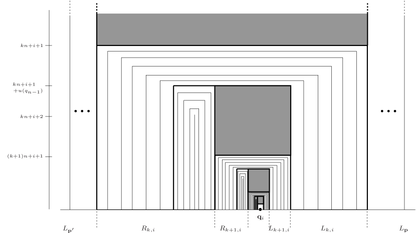
Figure 15. Strongly stable components in the rational general or late endpoint cases. The types of components are: (a) vertical lines $L_{{\mathbf{p}}}$ above the points ${\mathbf{p}}$ of the periodic orbit ${\mathbf{P}}$; (b) crosscuts $\Gamma^{\prime}(y,k,i)$ joining points of each $R_{k,i}$ to the corresponding points of $L_{k,i}$; (c) packets of crosscuts $\Gamma^{\prime}(y,k,i)$ above the subinterval of $R_{k,i}$ consisting of points which don’t correspond to points of $L_{k,i}$, together with the “central” arc $A_{k,i}$ which only intersects ${\widehat{S}}_{\infty}$ at a single point; and (d) the sets $D_{k,i}$ which consist of a shaded region together with the bold arcs connected to it, and which intersect ${\widehat{S}}_{\infty}$ at three points. The figure depicts the case where $q_{n-1}\in(c_{u},a)$; if $q_{n-1}\in(\alpha_{u},c_{u})$, then the packets of crosscuts are in $L_{k,i}$ rather than in $R_{k,i}$. The labeling on the $s$-axis is for the case $k\geq 0$.

Proof.

1. If ${\mathbf{p}}\in{\mathbf{P}}$ then ${\mathbf{p}}$ is landing of level 0, and the proof that $L_{{\mathbf{p}}}$ is strongly stable is identical to that of part (a) of Lemma 5.3.

2. Since $A_{k,i}=G^{kn+i}(A_{0,0})$, $\Gamma^{\prime}(y,k,i)=G^{kn+i}(\Gamma^{\prime}(y,0,0))$, and $D_{k,i}=G^{kn+i}(D_{0,0})$ for all $k\in{\mathbb{Z}}$, $0\leq i\leq n-1$, and $y\in(c_{u},a]\setminus\{\min(q_{n-1},{\widehat{q}}_{n-1})\}$, it suffices to consider the case $k=i=0$.

   That the sets $A_{0,0}$ and $\Gamma^{\prime}(y,0,0)$, and the crosscuts of $D_{0,0}$, are strongly stable is immediate from Lemma 4.57 and Remark 4.58, which gives that $\Psi(\eta)_{0}=b$ for all $\eta\in A_{0,0}$; $\Psi(\eta)_{0}=f(\tau(y))$ for all $\eta\in\Gamma^{\prime}(y,0,0)$; and $\Psi(\eta)_{0}=f(\tau(q_{n-1}))$ for all $\eta$ in the crosscuts of $D_{0,0}$.

   To complete the proof that $D_{0,0}$ is strongly stable, it is therefore only required to show that for all ${\mathbf{y}}\in[{\mathbf{t}}(a,1,0),\,{\mathbf{t}}(\alpha_{u},1,0)]$ and all $s\in[1+u(q_{n-1}),n+1]$ we have $\Psi({\mathbf{y}},s)_{0}=f(\tau(q_{n-1}))$. Given ${\mathbf{y}}\in[{\mathbf{t}}(a,1,0),\,{\mathbf{t}}(\alpha_{u},1,0)]=\{{\mathbf{q}}_{0}\}\cup\bigcup_{k=1}^{\infty}(L_{k,0}\cup R_{k,0})$, we have $y_{0}=q_{0}$ and $y_{r}=q_{n-r}$ for $1\leq r\leq n$. Since $y_{1}=q_{n-1}$ and $y_{1+i}\not\in{{\accentset{\circ}{\gamma}}}$ for $1\leq i\leq n-1$, Lemma 4.20 gives that $\Psi({\mathbf{y}},s)_{0}=f(\tau(q_{n-1}))$ for all $s\in[1+u(q_{n-1}),n+1]$ as required.

The proof that there are no connected strongly stable sets which strictly contain one of these sets proceeds in the same way as in the proof of Lemma 5.3. ∎

In the NBT case, where $q_{n-1}=c_{u}$, the interval $(c_{u},\min(q_{n-1},{\widehat{q}}_{n-1}))$ degenerates, leaving the simpler situation described in the following lemma, whose proof works in exactly the same way as that of Lemma 5.5. Its conclusions are illustrated by Figure 16.

Lemma 5.6.

Let $f$ be of rational NBT type, with $q(\kappa(f))=m/n\in(0,1/2)\cap{\mathbb{Q}}$. Then the strongly stable components of ${D^{{\scriptstyle\dagger}}}$ are $\{\partial^{\prime}\}$ and:

1. for each ${\mathbf{p}}\in{\mathbf{P}}$, the line $L_{{\mathbf{p}}}=\{{\mathbf{p}}\}\times(0,\infty]$;

2. for each $k\in{\mathbb{Z}}$ and $0\leq i\leq n-1$:

   1. for each $y\in(c_{u},a]$, the crosscut $\Gamma^{\prime}(y,k,i)$.

   2. the union $D_{k,i}$ of

      • the crosscut $\xi^{\prime}([{\mathbf{t}}(\alpha_{u},k+1,i),{\mathbf{t}}(a,k+1,i)],\,\,u_{k,i})$, and

      • the set $[{\mathbf{t}}(a,k+1,i),{\mathbf{t}}(\alpha_{u},k+1,i)]\,\,\times\,\,[u_{k,i},v_{k,i}]$.

      Here $u_{k,i}=\lambda^{kn+i}(2)$, $v_{k,i}=\lambda^{kn+i}(n+1)$, and both of the intervals in ${\widehat{S}}$ are those with the given endpoints which are disjoint from ${\mathbf{P}}$. ∎

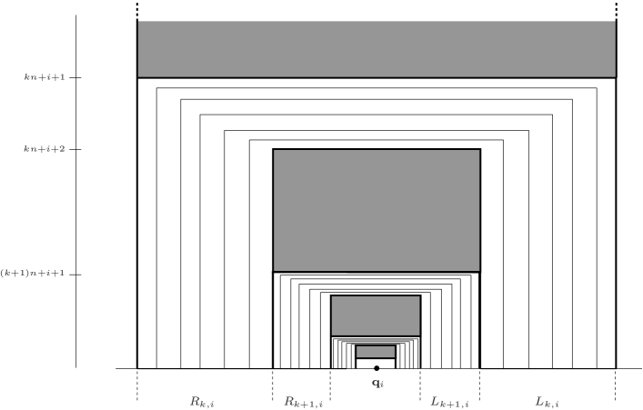
Figure 16. Strongly stable components in the rational NBT case. The packets of crosscuts which do not surround ${\mathbf{q}}_{i}$ have degenerated, and every component except for the lines $L_{\mathbf{p}}$ (${\mathbf{p}}\in{\mathbf{P}}$) touches ${\widehat{S}}_{\infty}$ at two points. The labeling on the $s$-axis is for the case $k\geq 0$.

In the rational normal endpoint case, on the other hand, the interval $(\min(q_{n-1},{\widehat{q}}_{n-1}),a]$ degenerates, giving rise to a more substantial modification to the description. The following lemma is illustrated by Figure 17.

Lemma 5.7.

Let $f$ be of rational normal endpoint type, with $q(\kappa(f))=m/n\in[0,1/2)\cap{\mathbb{Q}}$, and suppose that $f$ is of right hand endpoint type, so that $q_{n-1}=\alpha_{u}$ (the modifications in the left hand endpoint case are given at the end of the lemma statement). Then the strongly stable components of ${D^{{\scriptstyle\dagger}}}$ are $\{\partial^{\prime}\}$ and:

1. for each $k\in{\mathbb{Z}}$ and $0\leq i\leq n-1$:

   1. the arc $A_{k,i}=\{{\mathbf{t}}(c_{u},k,i)\}\times[r_{k,i},\infty]$, where $r_{k,i}=\lambda^{kn+i}(2)$, i.e.

      $$r_{k,i}=\begin{cases}kn+i+2&\text{ if }k\geq 0,\\ 1/2^{|k|n-i-1}&\text{ if }k<0.\end{cases}$$

   2. for each $y\in(c_{u},a)$, the crosscut $\Gamma^{\prime}(y,k,i)$.

2. For each $0\leq i\leq n-1$, the set

   $$D_{i}=L_{{\mathbf{q}}_{i}}\cup\bigcup_{k\in{\mathbb{Z}}}L_{{\mathbf{t}}(a,k,i)}\cup\bigcup_{k\in{\mathbb{Z}}}B_{k,i},$$

   where $L_{{\mathbf{y}}}$ is the line $\{{\mathbf{y}}\}\times(0,\infty]$ and $B_{k,i}=L_{k,i}\times(0,u_{k,i}]$ with $u_{k,i}=\lambda^{kn+i}(1)$, i.e.

   $$u_{k,i}=\begin{cases}kn+i+1&\text{ if }k\geq 0,\\ 1/2^{|k|n-i}&\text{ if }k<0.\end{cases}$$

In the left hand endpoint case $q_{n-1}=a$, the strongly stable components are given by replacing ${\mathbf{q}}_{i}$ with ${\mathbf{q}}_{i-m^{-1}\bmod n}$, ${\mathbf{t}}(a,k,i)$ with ${\mathbf{t}}(\alpha_{u},k,i)$, and $L_{k,i}$ with $R_{k,i}$ in (b).

Figure 17. Strongly stable components in the normal right hand endpoint case. The types of components are: (a) packets of crosscuts $\Gamma^{\prime}(y,k,i)$ above each interval $L_{k,i}$, together with the “central” arc $A_{k,i}$ which only intersects ${\widehat{S}}_{\infty}$ at a single point; and (b), for each $i$, the set $D_{i}$ consisting of the outermost crosscut above each $L_{k,i}$, the rectangles above these crosscuts extending up to (but not including) $s=0$, and the line $L_{{\mathbf{q}}_{i}}$ above ${\mathbf{q}}_{i}$. In the figure, $D_{0}$ is the union of the shaded region and all of the bold arcs: it intersects ${\widehat{S}}_{\infty}$ at infinitely many points.

Proof.

We suppose that $q_{n-1}=\alpha_{u}$, so that $m/n>0$. The modifications needed for the case $q_{n-1}=a$ are straightforward (including for the special sub-case $m/n=0$, when $q_{0}=a$ is fixed by $B$, and $\alpha_{u}=b$). Notice that, since the orbit of $a$ is disjoint from ${{\accentset{\circ}{\gamma}}}$, we have $\tau(B^{r}(a))=f^{r}(a)$ for all $r\geq 0$ by (3) (here the $a$ on the left hand side is $a\in S$, while the $a$ on the right hand side is $a\in I$). In particular, $f^{n}(a)=\tau(\alpha_{u})=\alpha$, $f(a)$ is periodic of period $n$, and $\tau(q_{i})=f^{i+1}(a)$ for $0\leq i\leq n-1$.

That the sets $A_{k,i}$ and $\Gamma^{\prime}(y,k,i)$ are strongly stable is immediate from Lemma 4.57 and Remark 4.58.

To show that the sets $D_{i}$ are strongly stable it suffices, since $G(D_{i})=D_{i+1\bmod n}$, to consider the case $i=0$.

1. Let ${\mathbf{y}}={\mathbf{q}}_{0}=\left<\left(q_{0},q_{n-1},q_{n-2},\ldots,q_{1}\right)^{\infty}\right>$. Since $y_{1}=q_{n-1}=\alpha_{u}$ and $y_{1+i}\not\in{{\accentset{\circ}{\gamma}}}$ for all $i\geq 1$, Lemma 4.20 gives that $\Psi({\mathbf{y}},s)_{0}=f(\tau(\alpha_{u}))=f(a)$ for all $s\in[1,\infty]$. On the other hand, if $s\in[1/2^{r},1/2^{r-1})$ for some $r\geq 1$, then $\Psi({\mathbf{y}},s)_{0}=(q_{0},s)$, and hence ${\widehat{H}}^{r}(\Psi({\mathbf{y}},s))_{0}=\tau(B^{r}(q_{0}))=\tau(q_{r\bmod n})=f^{r+1}(a)$. Therefore, for each $r\geq 0$,

   $${\widehat{H}}^{r}(\Psi({\mathbf{q}}_{0},s))_{0}=f^{r+1}(a)\qquad\text{ for all }s\in[1/2^{r},\infty].$$

2. By a similar argument applied to ${\mathbf{y}}={\mathbf{t}}(a,0,0)=\left<q_{0},a,B^{-1}(a),\ldots\right>$, we obtain that, for each $r\geq 0$, ${\widehat{H}}^{r}(\Psi({\mathbf{t}}(a,0,0),s))_{0}=f^{r+1}(a)\text{ for all }s\in[1/2^{r},\infty]$.

   Now for each $k\in{\mathbb{Z}}$ we have $G^{kn}({\mathbf{t}}(a,0,0),s)=({\mathbf{t}}(a,k,0),\lambda^{kn}(s))$. By Corollary 4.10, we obtain that for all $k\in{\mathbb{Z}}$ and all $r\geq 0$,

   $${\widehat{H}}^{r}(\Psi({\mathbf{t}}(a,k,0),s))_{0} = {\widehat{H}}^{r}(\Psi(G^{kn}({\mathbf{t}}(a,0,0),\lambda^{-kn}(s))))_{0}$$

   $$= {\widehat{H}}^{kn+r}(\Psi({\mathbf{t}}(a,0,0),\lambda^{-kn}(s)))_{0}$$

   $$= f^{kn}(f^{r+1}(a))=f^{r+1}(a)\qquad\text{ provided that }\lambda^{-kn}(s)\in[1/2^{r},\infty].$$

   Therefore, for each $k\in{\mathbb{Z}}$ and each $r\geq 0$, we have

   $${\widehat{H}}^{r}(\Psi({\mathbf{t}}(a,k,0),s))_{0}=f^{r+1}(a)\qquad\text{ for all }s\in[\lambda^{kn}(1/2^{r}),\infty].$$

3. Now let ${\mathbf{y}}={\mathbf{t}}(y,0,0)=\left<q_{0},y,B^{-1}(y),\ldots\right>\in L_{0,0}$, where $y\in[a,\alpha_{u})$. Then $\Psi({\mathbf{y}},1)_{0}=H(y,1/2)=f(a)$ by (8) and (U1) of Definition 3.2. On the other hand, if $s\in(0,1)$ we have $\Psi({\mathbf{y}},s)=\left<(q_{0},s),\ldots\right>$ and hence, as in (i), if $s\in[1/2^{r},1/2^{r-1})$ for some $r\geq 1$ then ${\widehat{H}}^{r}(\Psi({\mathbf{y}},s))_{0}=f^{r+1}(a)$. Therefore, for each $r\geq 0$,

   $${\widehat{H}}^{r}(\Psi({\mathbf{y}},s))_{0}=f^{r+1}(a)\qquad\text{ for all }s\in[1/2^{r},1]\text{ and all }{\mathbf{y}}\in L_{0,0}.$$

   Since $G^{kn}(L_{0,0})=L_{k,0}$ for each $k\in{\mathbb{Z}}$, a similar argument to that of part (ii) establishes that for all $k\in{\mathbb{Z}}$ and all $r\geq 0$,

   $${\widehat{H}}^{r}(\Psi({\mathbf{y}},s))_{0}=f^{r+1}(a)\qquad\text{ for all }s\in[\lambda^{kn}(1/2^{r}),u_{k,0}]\text{ and all }{\mathbf{y}}\in L_{k,0},$$

   where we have used that $\lambda^{kn}(1)=u_{k,0}$ for all $k\in{\mathbb{Z}}$.

Therefore, for all $\eta_{1},\eta_{2}\in D_{0}$, there is some $r\geq 0$ such that ${\widehat{H}}^{r}(\Psi(\eta_{1}))_{0}={\widehat{H}}^{r}(\Psi(\eta_{2}))_{0}=f^{r+1}(a)$, establishing that $D_{0}$ is strongly stable as required.

The proof that there are no connected strongly stable sets which strictly contain one of these sets proceeds in the same way as in the proof of Lemma 5.3. ∎

The quadratic-like strict left endpoint case (Section 4.7.2) is identical to the normal endpoint case, except that there are additional half-open intervals $I_{i}=\{{\mathbf{t}}(y)\,:\,y\in(q_{i},p_{i}]\}$ in ${\widehat{S}}$ (for $0\leq i\leq n-1$) whose points satisfy ${\widehat{B}}^{r}({\mathbf{t}}(y))_{0}\not\in\gamma$ for all $r\in{\mathbb{Z}}$. The strongly stable component containing $({\mathbf{t}}(y),\infty)$ is the line $\{{\mathbf{t}}(y)\}\times(0,\infty]$, exactly as in the irrational case; and other strongly stable components are as in the normal endpoint case. We therefore have the following description.

Lemma 5.8.

Let $f$ be of rational quadratic-like strict left endpoint type, with $q(\kappa(f))=m/n\in(0,1/2)\cap{\mathbb{Q}}$. Then the strongly stable components of ${D^{{\scriptstyle\dagger}}}$ are $\{\partial^{\prime}\}$ and:

1. for each $k\in{\mathbb{Z}}$ and $0\leq i\leq n-1$:

   1. the arc $A_{k,i}=\{{\mathbf{t}}(c_{u},k,i)\}\times[r_{k,i},\infty]$, where $r_{k,i}=\lambda^{kn+i}(2)$, i.e.

      $$r_{k,i}=\begin{cases}kn+i+2&\text{ if }k\geq 0,\\ 1/2^{|k|n-i-1}&\text{ if }k<0.\end{cases}$$

   2. for each $y\in(c_{u},a)$, the crosscut $\Gamma^{\prime}(y,k,i)$.

2. For each $0\leq i\leq n-1$, the set

   $$D_{i}=L_{{\mathbf{q}}_{i-m^{-1}\bmod{n}}}\cup\bigcup_{k\in{\mathbb{Z}}}L_{{\mathbf{t}}(\alpha_{u},k,i)}\cup\bigcup_{k\in{\mathbb{Z}}}B_{k,i},$$

   where $L_{{\mathbf{y}}}$ is the line $\{{\mathbf{y}}\}\times(0,\infty]$ and $B_{k,i}=R_{k,i}\times(0,u_{k,i}]$ with $u_{k,i}=\lambda^{kn+i}(1)$, i.e.

   $$u_{k,i}=\begin{cases}kn+i+1&\text{ if }k\geq 0,\\ 1/2^{|k|n-i}&\text{ if }k<0.\end{cases}$$

3. For each $0\leq i\leq n-1$ and each $y\in(q_{i},p_{i}]$, the line $L_{{\mathbf{t}}(y)}$.

The following straightforward consequence of the above proofs will be useful in Section 5.4.

Lemma 5.9.

1. Let $f$ be of irrational or rational early endpoint type. Then for each $r\geq 1$ and each $y\in(c_{u},a)$, the diameters of the strongly stable component images $\Psi(A_{r})$ and $\Psi(C_{r,y})$ are bounded above by $|b-a|/2^{r-1}$.

2. Let $f$ be of rational interior or late endpoint type with $q(\kappa(f))=m/n\in(0,1/2)\cap{\mathbb{Q}}$. Then for each $k\geq 0$, each $0\leq i\leq n-1$, and each $y\in(c_{u},a]\setminus\{\min(q_{n-1},{\widehat{q}}_{n-1})\}$, the diameters of the strongly stable component images $\Psi(A_{k,i})$, $\Psi(\Gamma^{\prime}(y,k,i))$ and $\Psi(D_{k,i})$ are bounded above by $|b-a|/2^{kn+i}$.

3. Let $f$ be of rational normal endpoint type or quadratic-like strict left endpoint type, with $q(\kappa(f))=m/n\in(0,1/2)\cap{\mathbb{Q}}$. Then for each $k\geq 0$, each $0\leq i\leq n-1$, and each $y\in(c_{u},a)$, the diameters of the strongly stable component images $\Psi(A_{k,i})$ and $\Psi(\Gamma^{\prime}(y,k,i))$ are bounded above by $|b-a|/2^{kn+i}$.

Proof.

In the irrational or early endpoint case, the proof of Lemma 5.3 shows that every element $\xi$ of $\Psi(A_{1})$ (respectively $\Psi(C_{1,y})$) has $\xi_{0}=b$ (respectively $\xi_{0}=f(\tau(y))$). Therefore any two elements of $\Psi(A_{r})$ or of $\Psi(C_{r,y})$ have equal $(r-1)^{\text{th}}$ entries, and so are within distance $|b-a|/2^{r-1}$ of each other. This establishes (a). Parts (b) and (c) follow similarly from the proofs of Lemmas 5.5 and 5.7, which show that every element $\xi$ of $\Psi(A_{0,0})$ (respectively $\Psi(\Gamma^{\prime}(y,0,0))$, $\Psi(D_{0,0})$) has $\xi_{0}=b$ (respectively $\xi_{0}=f(\tau(y))$, $\xi_{0}=f(\tau(q_{n-1}))$). ∎

5.3. Construction of the sphere homeomorphism

Definition 5.10 (The decomposition ${\mathcal{G}}^{\prime}$ of $\overline{D}$).

Let ${\mathcal{G}}^{\prime}$ be the decomposition of $\overline{D}$ whose elements are:

• $\{\eta\}$ for each $\eta\in\overline{D}\setminus{D^{{\scriptstyle\dagger}}}$;

• Strongly stable components whose closures don’t contain $\partial^{\prime}$; and

• The set $X$ which is the union of the strongly stable components whose closures contain $\partial^{\prime}$ (including the strongly stable component $\{\partial^{\prime}\}$ itself).

Remark 5.11.

It follows from the explicit descriptions of the strongly stable components that those whose closures don’t contain $\partial^{\prime}$ are compact; and that the set $X$ is also compact. Therefore ${\mathcal{G}}^{\prime}$ is the largest partition of $\overline{D}$ into compact sets with the property that every strongly stable component is contained in a single partition element.

Moreover, the elements of ${\mathcal{G}}^{\prime}$ are connected, and are permuted by $G$, since $G(X)=X$.

Lemma 5.12.

The restriction of $\Psi$ to each element of ${\mathcal{G}}^{\prime}$, apart from the single points of $\overline{D}\setminus{D^{{\scriptstyle\dagger}}}$ (where it is not defined), is a homeomorphism onto its image.

Proof.

This is immediate from the descriptions of the strongly stable components and Corollary 4.19 in all cases except for the element $X$ of ${\mathcal{G}}^{\prime}$ in the irrational, early endpoint, normal endpoint, and quadratic-like strict left endpoint cases.

Suppose that $f$ is of irrational type, so that the strongly stable components are given by Lemma 5.3. Then $X\cap{\widehat{S}}_{\infty}$ is the Cantor set $\Lambda_{\infty}$. $\Psi|_{X}$ is injective since $\Psi$ is injective on $D$ and on $\Lambda_{\infty}$ (Corollary 4.9 and Lemma 4.16), and $\Psi(\eta)\in{\widehat{I}}$ if and only if $\eta\in{\widehat{S}}_{\infty}$. Since $\Psi$ is continuous away from ${\widehat{S}}_{\infty}$ (Corollary 4.9), it is only necessary to show that $\Psi|_{X}$ is continuous at the points of $\Lambda_{\infty}$ (of course, $\Psi$ itself is not continuous at these points).

Now $\Psi|_{\Lambda\times[0,\infty]}$ is continuous by Lemma 4.17, since $\Lambda$ is uniformly landing of level 0. Thus it suffices to show that if $({\mathbf{y}},s)\in\bigcup_{r\in{\mathbb{Z}}}(G_{r}\times(0,u_{r}])$ is sufficiently close to a point $({\mathbf{y}}^{\prime},\infty)$ of $\Lambda_{\infty}$, then $\Psi({\mathbf{y}},s)$ is close to $\Psi({\mathbf{y}}^{\prime},\infty)$, where $G_{r}\times(0,u_{r}]$ are the rectangles of Lemma 5.3 (b)(iii). In order to do this we will show that, for all $N\geq 2$, if $({\mathbf{y}},s)\in G_{r}\times(0,u_{r}]$ for some $r$, and $s>N$, then $\Psi({\mathbf{y}},s)_{N-2}=\Psi({\mathbf{t}}(a,r),\infty)_{N-2}$. This will establish the result, since if $({\mathbf{y}},s)$ is close to $({\mathbf{y}}^{\prime},\infty)$ then $({\mathbf{t}}(a,r),\infty)\in\Lambda_{\infty}$ is also close to $({\mathbf{y}}^{\prime},\infty)$.

Recall that $u_{r}<1$ for $r<1$, and $u_{r}=r$ for $r\geq 1$. So if $({\mathbf{y}},s)\in G_{r}\times(0,u_{r}]$ and $s>N$, we have $N<s\leq r$. Observe that $G^{-(r-1)}({\mathbf{y}},s)=\left({\widehat{B}}^{-(r-1)}({\mathbf{y}}),\lambda^{-(r-1)}(s)\right)\in G_{1}\times(0,1]$.

Let $m\geq 0$ be such that $r-m\leq s<r-m+1$, so that $\lambda^{-(r-1)}(s)\in[1/2^{m},1/2^{m-1})$. By the proof of Lemma 5.3 (b)(iii), we have ${\widehat{H}}^{m}(\Psi(G^{-(r-1)}({\mathbf{y}},s)))_{0}=f^{m+1}(a)$: therefore, by Corollary 4.10, ${\widehat{H}}^{m-r+1}(\Psi({\mathbf{y}},s))_{0}=f^{m+1}(a)$, and so $\Psi({\mathbf{y}},s)_{r-m-1}=f^{m+1}(a)$. Since $r-m-1>s-2>N-2$, it follows that

$$\Psi({\mathbf{y}},s)_{N-2}=f^{r-(N-2)}(a)\qquad\text{ whenever }({\mathbf{y}},s)\in G_{r}\times(0,r]\text{ with }s>N.$$

On the other hand, $\Psi({\mathbf{t}}(a,r),\infty)=\omega({\mathbf{t}}(a,r))=\left<f^{r}(a),\ldots,f(a),a,\tau(B^{-1}(a)),\ldots\right>$ by (10), since ${\mathbf{t}}(a,r)\in{\mathcal{L}}_{r}$. Therefore $\Psi({\mathbf{t}}(a,r),\infty)_{N-2}=f^{r-(N-2)}(a)$, as required.

The proof when $f$ is of early endpoint type is identical, with the periodic orbit ${\mathbf{Q}}$ in place of the Cantor set $\Lambda$; and the proof when $f$ is of normal endpoint or quadratic-like strict left endpoint type involves only minor modifications. ∎

Definition 5.13 (The decomposition ${\mathcal{G}}$ of ${\widehat{T}}$).

Let ${\mathcal{G}}$ be the decomposition of ${\widehat{T}}$ whose elements are:

• the images under $\Psi$ of the elements of ${\mathcal{G}}^{\prime}$, other than points of $\overline{D}\setminus{D^{{\scriptstyle\dagger}}}$; and

• single points which are not in the image of $\Psi$.

By Corollary 4.10 and Remark 5.11, the elements of ${\mathcal{G}}$ are permuted by ${\widehat{H}}$.

Lemma 5.14.

${\mathcal{G}}$ is a non-separating monotone upper semi-continuous decomposition of ${\widehat{T}}$.

Proof.

The elements of ${\mathcal{G}}$ are compact, connected, and do not separate ${\widehat{T}}$ since the elements of ${\mathcal{G}}^{\prime}$ are compact, connected, and contractible, and the restriction of $\Psi$ to each of them is a homeomorphism by Lemma 5.12.

That ${\mathcal{G}}$ is upper semi-continuous is a special case of Lemma 5.26 below (where ${\mathcal{G}}$ is a single slice of a sliced decomposition which is shown to be upper semi-continuous). ∎

Theorem 5.15 (Semi-conjugacy to sphere homeomorphisms).

Let $f$ be a unimodal map satisfying the conditions of Convention 2.8. Then there is a sphere homeomorphism $F\colon\Sigma\to\Sigma$ and a continuous surjection $g\colon{\widehat{I}}\to\Sigma$ which semi-conjugates ${\widehat{f}}\colon{\widehat{I}}\to{\widehat{I}}$ to $F\colon\Sigma\to\Sigma$.

Every fiber of $g$ except for at most one contains three or fewer points, and only countably many fibers contain three points.

Proof.

By Lemma 5.14 and Moore’s theorem, $\Sigma={\widehat{T}}/{\mathcal{G}}$ is a sphere; and since ${\widehat{H}}$ permutes the elements of ${\mathcal{G}}$, the map $F={\widehat{H}}/{\mathcal{G}}\colon\Sigma\to\Sigma$ is a homeomorphism. Since every element of ${\mathcal{G}}$ intersects ${\widehat{I}}$, and ${\widehat{H}}|_{{\widehat{I}}}={\widehat{f}}$, it follows that $\Sigma$ is also the quotient of ${\widehat{I}}$ by the equivalence relation $\sim_{{\mathcal{G}}|_{{\widehat{I}}}}$ on ${\widehat{I}}$ induced by ${\mathcal{G}}$; and the canonical projection $g\colon{\widehat{I}}\to{\widehat{I}}/\!\!\sim_{{\mathcal{G}}|_{{\widehat{I}}}}=\Sigma$ is a semi-conjugacy between ${\widehat{f}}$ and $F$.

The statement about the cardinalities of the fibers of $g$ is immediate from the descriptions of the elements of ${\mathcal{G}}^{\prime}$ (Definition 5.10 and Lemmas 5.3, 5.5, 5.6, 5.7, and 5.8), every one of which except for $X$ intersects ${\widehat{S}}_{\infty}$ in three or fewer points, and only countably many of which can intersect ${\widehat{S}}_{\infty}$ in three points. ∎

Remark 5.16.

Since $\Psi|_{X}$ is a homeomorphism onto its image (Lemma 5.12), the restriction of ${\widehat{f}}$ to the exceptional fiber $\Psi(X\cap{\widehat{S}}_{\infty})$ of $g$ is topologically conjugate to the action of the circle homeomorphism ${\widehat{B}}$ on an invariant subset in the circle, and therefore has topological entropy zero. It follows from a result of Bowen (Theorem 17 of [13]), using the fact that all other fibers are finite, that ${\widehat{f}}\colon{\widehat{I}}\to{\widehat{I}}$ and $F\colon\Sigma\to\Sigma$ have the same topological entropy. Since ${\widehat{f}}$ and $f$ also have the same topological entropy (this follows from the same result of Bowen), we conclude that the sphere homeomorphism $F\colon\Sigma\to\Sigma$ has the same topological entropy as the unimodal map $f\colon I\to I$.

Remark 5.17.

By the proof of Theorem 5.15, the fibers of the semi-conjugacy $g\colon{\widehat{I}}\to\Sigma$ can be described explicitly. Every non-trivial fiber is contained in the set of accessible points and, conversely, all but countably many trivial fibers are contained in the set of inaccessible points.

The accessible fibers of $g$ are as follows:

1. In the irrational case, there is one fiber equal to $\omega(\Lambda)$, where $\Lambda$ is the Cantor set of Definition 4.41; and there are countably many accessible trivial fibers $\{\omega({\mathbf{t}}(c_{u},r))\}$ for $r\in{\mathbb{Z}}$. All other accessible fibers are of the form $\{\omega({\mathbf{t}}(y,r)),\omega({\mathbf{t}}({\widehat{y}},r))\}$, where $y\in{{\accentset{\circ}{\gamma}}}\setminus\{c_{u}\}$ and $r\in{\mathbb{Z}}$.

2. In the early endpoint case there is one fiber

   $$\omega({\widehat{S}}_{\infty})\setminus\{\omega({\mathbf{t}}(y,r))\,:\,y\in{{\accentset{\circ}{\gamma}}},r\in{\mathbb{Z}}\}$$

   which is either a countable union of disjoint intervals, or such a union together with finitely many isolated points; and there are countably many accessible trivial fibers $\{\omega({\mathbf{t}}(c_{u},r))\}$ for $r\in{\mathbb{Z}}$. All other accessible fibers are of the form $\{\omega({\mathbf{t}}(y,r)),\omega({\mathbf{t}}({\widehat{y}},r))\}$, where $y\in{{\accentset{\circ}{\gamma}}}\setminus\{c_{u}\}$ and $r\in{\mathbb{Z}}$.

3. In the normal endpoint case with $q(\kappa(f))=m/n$ there is one countable fiber

   $$\omega({\mathbf{Q}})\,\cup\,\{\omega({\mathbf{t}}(A,k,i))\,:\,k\in{\mathbb{Z}},\,0\leq i\leq n-1\},$$

   where $A=a$ if $\kappa(f)=\operatorname{rhe}(m/n)$, and $A=\alpha_{u}$ if $\kappa(f)=\operatorname{lhe}(m/n)$; and there are countably many accessible trivial fibers $\{\omega({\mathbf{t}}(c_{u},k,i))\}$ for $k\in{\mathbb{Z}}$ and $0\leq i\leq n-1$. All other accessible fibers are of the form $\{\omega({\mathbf{t}}(y,k,i)),\omega({\mathbf{t}}({\widehat{y}},k,i))\}$, where $y\in{{\accentset{\circ}{\gamma}}}\setminus\{c_{u}\}$, $k\in{\mathbb{Z}}$ and $0\leq i\leq n-1$.

4. In the quadratic-like strict left end point case with $q(\kappa(f))=m/n$, there is one fiber

   $$\omega({\mathbf{Q}})\cup\bigcup_{i=0}^{n-1}\omega(I_{i})\cup\{\omega({\mathbf{t}}(\alpha_{u},k,i))\,:\,k\in{\mathbb{Z}},0\leq i\leq n-1\}$$

   which is the union of $n$ disjoint compact intervals and countably many points; and there are countably many accessible trivial fibers $\{\omega({\mathbf{t}}(c_{u},k,i))\}$ for $k\in{\mathbb{Z}}$ and $0\leq i\leq n-1$. All other accessible fibers are of the form $\{\omega({\mathbf{t}}(y,k,i)),\omega({\mathbf{t}}({\widehat{y}},k,i))\}$, where $y\in{{\accentset{\circ}{\gamma}}}\setminus\{c_{u}\}$, $k\in{\mathbb{Z}}$ and $0\leq i\leq n-1$.

5. In the rational general and late endpoint cases with $q(\kappa(f))=m/n$, there is one fiber $\omega({\mathbf{P}})$ of cardinality $n$; countably many $3$-element fibers of the form

   $$\{\omega({\mathbf{t}}({\widehat{q}}_{n-1},k,i)),\omega({\mathbf{t}}(a,k+1,i)),\omega({\mathbf{t}}(\alpha_{u},k+1,i))\}\quad\text{ for $k\in{\mathbb{Z}}$ and $0\leq i\leq n-1$};$$

   and countably many accessible trivial fibers $\{\omega({\mathbf{t}}(c_{u},k,i))\}$ for $k\in{\mathbb{Z}}$ and $0\leq i\leq n-1$. All other accessible fibers are of the form $\{\omega({\mathbf{t}}(y,k,i)),\omega({\mathbf{t}}({\widehat{y}},k,i))\}$, where $y\in{{\accentset{\circ}{\gamma}}}\setminus\{q_{n-1},{\widehat{q}}_{n-1},c_{u}\}$, $k\in{\mathbb{Z}}$, and $0\leq i\leq n-1$.

6. In the rational NBT case with $q(\kappa(f))=m/n$, there is one fiber $\omega({\mathbf{P}})$ of cardinality $n$. All other accessible fibers are of the form $\{\omega({\mathbf{t}}(y,k,i)),\omega({\mathbf{t}}({\widehat{y}},k,i))\}$, where $y\in\gamma\setminus\{c_{u}\}$, $k\in{\mathbb{Z}}$, and $0\leq i\leq n-1$.

Note that the exceptional fiber of $g$ can only be infinite when $f$ is of irrational or endpoint type. In particular, for the tent family $\{f_{t}\}$, the semi-conjugacy has only finite fibers for an open dense subset of parameters.

An immediate consequence of Theorem 5.15 is that any unimodal map with topological entropy greater than $\frac{1}{2}\log 2$ has natural extension semi-conjugate to a sphere homeomorphism, although the fibers of the semi-conjugacy may not be so well behaved when the conditions of Convention 2.8 are not satisfied.

Corollary 5.18.

Let $f$ be any unimodal map (not necessarily satisfying the conditions of Convention 2.8) with topological entropy $h(f)>\frac{1}{2}\log 2$. Then the natural extension ${\widehat{f}}$ is semi-conjugate to a sphere homeomorphism with the same topological entropy as $f$.

Proof.

$h(f)>\frac{1}{2}\log 2$ is equivalent to $\kappa(f)\succ 101^{\infty}$. Now $f$ is semi-conjugate to a tent map $F$ with $\kappa(F)=\kappa(f)$ and $h(F)=h(f)$ (see [31, 36]), and hence ${\widehat{f}}\colon{\widehat{I}}_{f}\to{\widehat{I}}_{f}$ is semi-conjugate to ${\widehat{F}}\colon{\widehat{I}}_{F}\to{\widehat{I}}_{F}$, which is semi-conjugate to a sphere homeomorphism of topological entropy $h(F)$ by Theorem 5.15 and Remark 5.16. ∎

5.4. Continuously varying families

Our aim in this section is the following result, which shows that the above construction of sphere homeomorphisms can be carried out continuously.

Theorem 5.19.

Let $J$ be a compact parameter interval, and $\{f_{t}\}_{t\in J}$ be a continuously varying family of unimodal maps, all of which are defined on the same core interval $I$ and satisfy the conditions of Convention 2.8. For each $t$, let $F_{t}\colon\Sigma_{t}\to\Sigma_{t}$ be the sphere homeomorphism constructed from $f_{t}$ in the proof of Theorem 5.15. Then there is a continuously varying family $\{\chi_{t}\colon S^{2}\to S^{2}\}_{t\in J}$ of sphere homeomorphisms such that $\chi_{t}$ is topologically conjugate to $F_{t}$ for each $t$.

In particular, each natural extension ${\widehat{f}}_{t}\colon{\widehat{I}}_{t}\to{\widehat{I}}_{t}$ is semi-conjugate to $\chi_{t}$, by a semi-conjugacy all but one of whose fibers contains three or fewer points, and only countably many of whose fibers contain three points.

Remark 5.20.

If $f_{t}\colon I_{t}\to I_{t}$, where $\{I_{t}\}$ is a continuously varying family of compact intervals — as occurs naturally when families of unimodal maps are restricted to their core intervals — then the theorem applies after conjugating by a continuously varying affine coordinate change.

Throughout this section, $\{f_{t}\}_{t\in J}$ will denote a fixed family of unimodal maps as in the statement of Theorem 5.19. Because the domain $I=[a,b]$ is fixed, the circle $S$ and the sphere $T$ are independent of the parameter $t$. However, almost every other object is parameter dependent. This dependence will generally be indicated with a subscript $t$, but will sometimes be suppressed, particularly when it doesn’t serve to illuminate continuity or convergence arguments, in order to avoid excessive notation. For example, we will not normally make explicit the parameter dependence of $c_{u}$ and $\alpha_{u}$.

Recall that $\{\overline{f}_{t}\colon T\to T\}$ is a continuously varying family of unwrappings of $\{f_{t}\}$, and that the homeomorphisms ${\widehat{H}}_{t}\colon{\widehat{T}}_{t}\to{\widehat{T}}_{t}$ are the natural extensions of the near-homeomorphisms

$$H_{t}=\Upsilon\circ\overline{f}_{t}\colon T\to T.$$

Let

$${\widehat{T}}_{\ast}=\bigsqcup_{t\in J}\left({\widehat{T}}_{t}\times\{t\}\right),$$

topologized as a compact subset of $T^{\mathbb{N}}\times J$. The following result from [14] — which is the key lemma used in the proof of Theorem 2.14 — tells us that ${\widehat{T}}_{\ast}$ is homeomorphic to $S^{2}\times J$.

Theorem 5.21.

There is a slice-preserving homeomorphism $\beta\colon{\widehat{T}}_{\ast}\to T\times J$.

Here slice-preserving means that $\beta({\widehat{T}}_{t}\times\{t\})=T\times\{t\}$ for each $t$. In [14] this result is stated not for ${\widehat{T}}_{\ast}$, but for the inverse limit $\widehat{T\times J}$ of the fat map $T\times J\to T\times J$ defined by $(x,t)\mapsto(H_{t}(x),t)$. However ${\widehat{T}}_{\ast}$ and $\widehat{T\times J}$ are homeomorphic by the slice-preserving homeomorphism $\left(\left<x_{0},x_{1},\ldots\right>,t\right)\mapsto\left<(x_{0},t),(x_{1},t),\ldots\right>$.

Let ${\widehat{H}}_{\ast}\colon{\widehat{T}}_{\ast}\to{\widehat{T}}_{\ast}$ be the slice-preserving homeomorphism defined by ${\widehat{H}}_{\ast}({\mathbf{x}},t)=({\widehat{H}}_{t}({\mathbf{x}}),t)$, and ${\mathcal{G}}_{\ast}$ be the ${\widehat{H}}_{\ast}$-invariant decomposition of ${\widehat{T}}_{\ast}$ induced in each slice by ${\mathcal{G}}_{t}$: that is,

$${\mathcal{G}}_{\ast}=\{g\times\{t\}\,:\,t\in J\text{ and }g\in{\mathcal{G}}_{t}\}.$$

The elements of ${\mathcal{G}}_{\ast}$ are each contained in a slice of ${\widehat{T}}_{\ast}$, and moreover are compact, connected, and do not separate their slices, since these properties are inherited from the ${\mathcal{G}}_{t}$ (see Lemma 5.14). Lemma 5.26 below states that ${\mathcal{G}}_{\ast}$ is upper semi-continuous. We now assume this lemma and show how to complete the proof of the Theorem 5.19. The key ingredient is the following theorem of Dyer and Hamstrom [23] (both statement and proof of this result are contained in the proof of Theorem 8 of [23]: note that a decomposition is upper semi-continuous if and only if its quotient mapping is closed).

Theorem 5.22 (Dyer – Hamstrom).

Let ${\mathcal{G}}$ be a monotone upper semi-continuous decomposition of $S^{2}\times J$ into compact subsets, each of whose elements lies in, and does not separate, some slice $S^{2}\times\{t\}$. Suppose also that there is an arc $L$ in $S^{2}\times J$ which intersects each slice $S^{2}\times\{t\}$ in a singleton decomposition element. Then there is a slice-preserving homeomorphism $K\colon(S^{2}\times J)/{\mathcal{G}}\to S^{2}\times J$.

It follows that, assuming the upper semi-continuity of ${\mathcal{G}}_{\ast}$, we have the commutative diagram of Figure 18. Here $\pi$ is the quotient mapping of the decomposition ${\mathcal{G}}_{\ast}$; $K$ is the homeomorphism of Theorem 5.22 (which exists since, by Theorem 5.21, ${\widehat{T}}_{\ast}$ is slice-preserving homeomorphic to $S^{2}\times J$: a suitable arc $L$ is the one which intersects each ${\widehat{T}}_{t}\times\{t\}$ at $({\mathbf{z}}_{t},t)$, where ${\mathbf{z}}_{t}\in{\widehat{I}}_{t}$ is the fixed point of ${\widehat{H}}_{t}$ which lies above the fixed point $z_{t}$ of $f_{t}$ in $(c,b)$); and ${\widehat{H}}_{\ast}/{\mathcal{G}}_{\ast}$, and $\chi_{\ast}$ are the homeomorphisms which make the diagram commute. All of the maps in the diagram are slice-preserving, and in particular $\chi_{\ast}\colon S^{2}\times J\to S^{2}\times J$ defines a continuously varying family $\{\chi_{t}\}_{t\in J}$ of sphere homeomorphisms. Restricting the diagram to a single slice, we see that $\chi_{t}$ is topologically conjugate to the homeomorphism $F_{t}={\widehat{H}}_{t}/{\mathcal{G}}_{t}$ of Theorem 5.15, which completes the proof of Theorem 5.19.

$$\begin{CD}{\widehat{T}}_{\ast}@>{{\widehat{H}}_{\ast}}>{}>{\widehat{T}}_{\ast}\\ @V{\pi}V{}V@V{}V{\pi}V\\ {\widehat{T}}_{\ast}/{\mathcal{G}}_{\ast}@>{{\widehat{H}}_{\ast}/{\mathcal{G}}_{\ast}}>{}>{\widehat{T}}_{\ast}/{\mathcal{G}}_{\ast}\\ @V{K}V{}V@V{}V{K}V\\ S^{2}\times J@>{\chi_{\ast}}>{}>S^{2}\times J.\\ \end{CD}$$

Figure 18. Construction of the continuous family of sphere homeomorphisms.

It therefore only remains to show that the decomposition ${\mathcal{G}}_{\ast}$ of ${\widehat{T}}_{\ast}$ is upper semi-continuous. We do this by first considering the decompositions ${\mathcal{G}}^{\prime}_{t}$ of the spaces $\overline{D}_{t}$ — which are described explicitly by Lemmas 5.3, 5.5, 5.6, 5.7, and 5.8 — and then transferring the results using the maps $\Psi_{t}$.

Recall from Definition 5.10 that, for each $t\in J$, the decomposition ${\mathcal{G}}^{\prime}_{t}$ of $\overline{D}_{t}$ has as elements

• Strongly stable components whose closures are disjoint from $\partial^{\prime}_{t}$,

• The union $X_{t}$ of strongly stable components whose closures contain $\partial^{\prime}_{t}$, and

• Single points at which $\Psi_{t}$ is not defined.

We write

$$\overline{D}_{\ast}=\bigsqcup_{t\in J}\left(\overline{D}_{t}\times\{t\}\right),$$

topologized as a compact subset of $\left(S^{\mathbb{N}}\times[0,\infty]\right)/\left(S^{\mathbb{N}}\times\{0\}\right)\,\times\,J$, and define

$${\mathcal{G}}^{\prime}_{\ast}=\{g^{\prime}\times\{t\}\,:\,t\in J\text{ and }g^{\prime}\in{\mathcal{G}}^{\prime}_{t}\}$$

to be the sliced decomposition of $\overline{D}_{\ast}$ induced on each slice by the decompositions ${\mathcal{G}}^{\prime}_{t}$.

Recall also (Definitions 4.11) that, for each $t$, we denote by ${D^{{\scriptstyle\dagger}}_{{t}}}$ the subset of $\overline{D}_{t}$ on which $\Psi_{t}$ is defined: that is, ${D^{{\scriptstyle\dagger}}_{{t}}}=\overline{D}_{t}$ if $f_{t}$ is of irrational or rational endpoint type, and otherwise ${D^{{\scriptstyle\dagger}}_{{t}}}=\overline{D}_{t}\setminus{\mathbf{Q}}_{t}$. Writing ${D^{{\scriptstyle\dagger}}_{\ast}}$ for the subset $\bigsqcup_{t\in J}({D^{{\scriptstyle\dagger}}_{{t}}}\times\{t\})$ of $\overline{D}_{\ast}$, we can then define the function $\Psi_{\ast}\colon{D^{{\scriptstyle\dagger}}_{\ast}}\to{\widehat{T}}_{\ast}$ by $\Psi_{\ast}(\eta,t)=(\Psi_{t}(\eta),t)$. With these definitions, the non-trivial elements of the decomposition ${\mathcal{G}}_{\ast}$ of ${\widehat{T}}_{\ast}$ are precisely the images under $\Psi_{\ast}$ of the non-trivial elements of ${\mathcal{G}}^{\prime}_{\ast}$.

The proof of the following is essentially the same as that of Corollary 4.9.

Lemma 5.23.

$\Psi_{\ast}$ is continuous at $\left(({\mathbf{y}},s),t\right)\in{D^{{\scriptstyle\dagger}}_{\ast}}$ whenever $s<\infty$.

Proof.

For each $N\in{\mathbb{N}}$, we have that, whenever $s<N+1$,

$$\Psi_{\ast}\left(({\mathbf{y}},s),t\right)=\left<H_{t}^{N}(y_{N},\lambda^{-N}(s)),H_{t}^{N}(y_{N+1},\lambda^{-(N+1)}(s)),\ldots\right>$$

by (9), (6), and (4). This expression is clearly continuous in $\left(({\mathbf{y}},s),t\right)$. ∎

The main technique in the proof of upper semi-continuity of ${\mathcal{G}}_{\ast}$ is to take certain convergent sequences in ${\widehat{T}}_{\ast}$, transfer them to ${D^{{\scriptstyle\dagger}}_{\ast}}$ using $\Psi_{\ast}^{-1}$, draw conclusions about the limit in ${D^{{\scriptstyle\dagger}}_{\ast}}$, and transfer back to ${\widehat{T}}_{\ast}$. In order to do this, we need to know that $\Psi_{\ast}$ respects the limits of certain sequences, although it may not be continuous at those limits. The following lemma enables us to do this: parts (a) and (b) are natural, while part (c), which is more esoteric, is motivated by the specific requirements of the proof.

Lemma 5.24.

Let $\left(({\mathbf{y}}^{(j)},s_{j}),t_{j}\right)\to\left(({\mathbf{y}},s),t\right)$ be a convergent sequence in ${D^{{\scriptstyle\dagger}}_{\ast}}$. Then $\Psi_{\ast}\left(({\mathbf{y}}^{(j)},s_{j}),t_{j}\right)\to\Psi_{\ast}\left(({\mathbf{y}},s),t\right)$ if one of the following holds:

1. $s<\infty$;

2. ${\mathbf{y}}$ and all of the ${\mathbf{y}}^{(j)}$ are landing of level $1$; or

3. ${\mathbf{y}}$ is landing of level 1, and there is a sequence $n_{j}\to\infty$ such that for each $j$ we have $s_{j}\leq n_{j}+1$ and $y^{(j)}_{i}\not\in{{\accentset{\circ}{\gamma}}}_{t_{j}}$ for $2\leq i\leq n_{j}$.

Proof.

1. By Lemma 5.23.

2. We can assume that $s=\infty$ since otherwise (a) applies. Fix $r\geq 1$. Since ${\mathbf{y}}\in{\mathcal{L}}_{r}$, Corollary 4.14 gives $\Psi_{t}({\mathbf{y}},\infty)_{r}=\tau(y_{r})$; and since ${\mathbf{y}}^{(j)}\in{\mathcal{L}}_{r}$, Lemma 4.13 gives $\Psi_{t_{j}}({\mathbf{y}}^{(j)},s_{j})_{r}=\tau(y^{(j)}_{r})$, provided that $j$ is large enough that $s_{j}\geq r+1$. Therefore for each $r\geq 1$ we have $\Psi_{t_{j}}({\mathbf{y}}^{(j)},s_{j})_{r}\to\Psi_{t}({\mathbf{y}},\infty)_{r}$ as $j\to\infty$, and the result follows.

3. We can again assume that $s=\infty$. Fix $r\geq 1$. As for (b), we have $\Psi_{t}({\mathbf{y}},\infty)_{r}=\tau(y_{r})$. For each $j$ large enough that $n_{j}\geq r+2$, we have $y^{(j)}_{(r+1)+i}\not\in{{\accentset{\circ}{\gamma}}}_{t_{j}}$ for $1\leq i\leq n_{j}-(r+1)$, so that Lemma 4.20 gives

   $$\Psi_{t_{j}}({\mathbf{y}}^{(j)},s^{\prime})_{r}=f_{t_{j}}(\tau(y^{(j)}_{r+1}))=\tau(y^{(j)}_{r})\quad\text{ for all }s^{\prime}\in[r+2,n_{j}+1].$$

   In particular, since $s_{j}\leq n_{j}+1$ for all $j$, we have $\Psi_{t_{j}}({\mathbf{y}}^{(j)},s_{j})_{r}=\tau(y^{(j)}_{r})$ whenever $j$ is large enough that $s_{j}\geq r+2$, so that $\Psi_{t_{j}}({\mathbf{y}}^{(j)},s_{j})_{r}\to\Psi_{t}({\mathbf{y}},\infty)_{r}$ as $j\to\infty$.

∎

The following abbreviated language will be convenient.

Definition 5.25 (Type and height of a parameter).

We say that a parameter $t\in J$ is of irrational, rational, and rational interior, early endpoint, normal endpoint, quadratic-like strict left endpoint, or late endpoint type according as $f_{t}$ is. We define the height of $t$ to be $q(\kappa(f_{t}))$.

Lemma 5.26.

The decomposition ${\mathcal{G}}_{\ast}$ of ${\widehat{T}}_{\ast}$ is upper semi-continuous.

Proof.

Let $(t_{j})$ be a sequence in $J$ converging to $t\in J$, and for each $j$, let $g_{j}$ be a decomposition element of ${\mathcal{G}}_{t_{j}}$. We need to show that there is a decomposition element $g\in{\mathcal{G}}_{t}$ with the property that, whenever $(\xi_{j},t_{j})$ is a sequence in ${\widehat{T}}_{\ast}$ with $(\xi_{j},t_{j})\to(\xi,t)$ and $\xi_{j}\in g_{j}$ for all $j$, then we have $\xi\in g$.

This is clearly the case if infinitely many of the $g_{j}$ are singletons, so we can assume that there are decomposition elements $g_{j}^{\prime}\in{\mathcal{G}}^{\prime}_{t_{j}}$ with $\Psi_{t_{j}}(g_{j}^{\prime})=g_{j}$ for each $j$.

Observe that if the required property holds for some subsequence of $(t_{j},g_{j})$, then it also holds for the full sequence. By taking such a subsequence, we can therefore further assume that all of the $t_{j}$ are of rational interior or late endpoint type (type A); or that they are all of rational normal or quadratic-like endpoint type (type B); or that they are all of irrational or rational early endpoint type (type C). We will consider each of these three cases in turn. The arguments will also depend on the type of the limiting parameter $t$. We note that $t$ can only be of type A if the $t_{j}$ are also of type A, and if the sequence $m_{j}/n_{j}$ of their heights is eventually constant, since the set $J_{q}$ of parameters $t$ of rational interior or late endpoint type with prescribed height $q$ is open in $J$. This is because $J_{q}=\{t\in J\,:\,(w_{q}1)^{\infty}\prec\kappa(f_{t})\prec 10({\widehat{w}}_{q}1)^{\infty}\}$ (see Definitions 2.23 and 2.25); because if $\kappa(f_{t})=(w_{q}0)^{\infty}$ then the turning point of $f_{t}$ is not periodic by Definition 2.4; and because $10({\widehat{w}}_{q}1)^{\infty}$ is not a periodic sequence by Lemma 2.22 (d).

The method of proof is the same in all three cases. We first use the explicit description of the decompositions ${\mathcal{G}}^{\prime}_{t}$ provided by Lemmas 5.3, 5.5, 5.6, 5.7, and 5.8 to show that either (i) the diameters of (a subsequence of) the decomposition elements $g_{j}$ converge to zero, in which case the result is obvious; or (ii) there is a decomposition element $g^{\prime}\in{\mathcal{G}}^{\prime}_{t}$ with the property that, whenever $(\eta_{j},t_{j})$ is a sequence in ${D^{{\scriptstyle\dagger}}_{\ast}}$ with $(\eta_{j},t_{j})\to(\eta,t)$ and $\eta_{j}\in g_{j}^{\prime}$ for all $j$, we have $\eta\in g^{\prime}$. Then if $(\xi_{j},t_{j})\to(\xi,t)$ with $\xi_{j}\in g_{j}$ for all $j$, we define $\eta_{j}=\Psi_{t_{j}}^{-1}(\xi_{j})\in g_{j}^{\prime}$, and take a subsequence if necessary to ensure that $(\eta_{j},t_{j})\to(\eta,t)$ with $\eta\in g^{\prime}$. Writing $g=\Psi_{t}(g^{\prime})$, it only remains to show, using Lemma 5.24, that $(\xi_{j},t_{j})=\Psi_{\ast}(\eta_{j},t_{j})\to\Psi_{\ast}(\eta,t)$, so that $\xi\in g$ as required.

We will therefore assume, in each case, that $(\eta_{j},t_{j})=\left(({\mathbf{y}}^{(j)},s_{j}),t_{j}\right)\to(\eta,t)=\left(({\mathbf{y}},s),t\right)$ is a sequence in ${D^{{\scriptstyle\dagger}}_{\ast}}$, and show that the decomposition element $g^{\prime}\in{\mathcal{G}}^{\prime}_{t}$ which contains $\eta$ only depends on the decomposition elements $g^{\prime}_{j}\in{\mathcal{G}}^{\prime}_{t_{j}}$ which contain the $\eta_{j}$. The proof in the given case will then be completed by showing (or observing) that one of the conditions of Lemma 5.24 holds.

The decomposition elements $X_{t}\in{\mathcal{G}}^{\prime}_{t}$ (see Definition 5.10) which contain $\partial^{\prime}$ play a special role in the arguments. Observe that in all cases these contain the verticals $\{{\mathbf{y}}\}\times[0,\infty]$ above the points ${\mathbf{y}}\in{\widehat{S}}_{t}$ which have the property that ${\widehat{B}}^{r}_{t}({\mathbf{y}})_{0}\not\in{{\accentset{\circ}{\gamma}}}_{t}$ for all $r\in{\mathbb{Z}}$; and that in the rational interior and late endpoint cases, $X_{t}$ is equal to the union of these verticals.

If infinitely many of the $s_{j}$ are equal to $0$ then $s=0$, and hence (using Lemma 5.24 (a)), $\xi\in\Psi_{t}(X_{t})$. We will therefore always assume that $s>0$ and that $s_{j}>0$ for all $j$.

Sequences of type A are the hardest to treat, mainly because there are decomposition elements (other than $X_{t})$ which are not uniformly landing. They also involve the most subcases, since limits of type A are possible, and because limits of type B can be approached in two quite different ways, either from within their height interval or from outside it. We will treat this case in detail — although methods of arguments will be successively abbreviated as they recur — and treat sequences of types B and C more briefly. Although the proof is quite long, it involves nothing more than the careful enumeration of cases and their analysis using the explicit description of the decomposition ${\mathcal{G}}^{\prime}_{\ast}$.

Case A: All $t_{j}$ are of rational interior or late endpoint type.

In this case the decompositions ${\mathcal{G}}^{\prime}_{t_{j}}$ are given by Lemma 5.5 or, in the NBT case, by Lemma 5.6. Let the height of $t_{j}$ be $m_{j}/n_{j}$. Suppose first that infinitely many (and so, without loss of generality, all) of the $\eta_{j}$ are contained in the $n_{j}$-stars $X_{t_{j}}$, so that for each $j$ we have ${\widehat{B}}^{r}_{t_{j}}({\mathbf{y}}^{(j)})_{0}\not\in{{\accentset{\circ}{\gamma}}}_{t_{j}}$ for all $r\in{\mathbb{Z}}$. Since ${\widehat{B}}_{t}$ and $\gamma_{t}$ vary continuously with $t$, it follows that ${\widehat{B}}^{r}_{t}({\mathbf{y}})_{0}\not\in{{\accentset{\circ}{\gamma}}}_{t}$ for all $r\in{\mathbb{Z}}$: therefore $\eta\in X_{t}$. Observing that ${\mathbf{y}}$ and ${\mathbf{y}}^{(j)}$ are landing of level 0, and hence of level 1, completes the proof using Lemma 5.24 (b).

We can therefore assume that none of the $\eta_{j}$ lie in $X_{t_{j}}$, and so can define $k_{j}\in{\mathbb{Z}}$ and $0\leq i_{j}\leq n_{j}-1$ such that

$$\eta_{j}\in A_{k_{j},i_{j}}\cup D_{k_{j},i_{j}}\cup\bigcup_{y\in(c_{u},a]\setminus\{\min(q_{n_{j}-1},{\widehat{q}}_{n_{j}-1})\}}\Gamma^{\prime}(y,k_{j},i_{j})$$

for each $j$, where $A_{k_{j},i_{j}}$, $D_{k_{j},i_{j}}$, and $\Gamma^{\prime}(y,k_{j},i_{j})$ are the elements of ${\mathcal{G}}^{\prime}_{t_{j}}$ defined in the statements of Lemmas 5.5 and 5.6 (we suppress the dependence of these decomposition elements, as well as that of $c_{u}$ and $q_{n_{j}-1}$, on $t_{j}$).

There are three possibilities:

1. The sequence $(n_{j}k_{j}+i_{j})$ is not bounded above. Then, by Lemma 5.9 (b), there is a subsequence of the $\xi_{j}=\Psi_{t_{j}}(\eta_{j})$ contained in decomposition elements whose diameters go to zero.

2. The sequence $(n_{j}k_{j}+i_{j})$ is not bounded below so that, taking a subsequence, we can assume that $k_{j}<0$ for all $j$ and that $n_{j}k_{j}+i_{j}\to-\infty$. For each $j$, we therefore have either that ${\widehat{B}}^{r}_{t_{j}}({\mathbf{y}}^{(j)})_{0}\not\in{{\accentset{\circ}{\gamma}}}_{t_{j}}$ for all $r\in{\mathbb{Z}}$ with $r\leq-(n_{j}k_{j}+i_{j}+1)$, or that $s_{j}\leq 2^{n_{j}k_{j}+i_{j}+1}$ (depending on whether $\eta_{j}$ is in a vertical of its decomposition element, or is in one of the horizontals, or disks of $D_{k_{j},i_{j}}$). Since $s\not=0$ it follows that ${\widehat{B}}^{r}_{t}({\mathbf{y}})_{0}\not\in{{\accentset{\circ}{\gamma}}}_{t}$ for all $r\in{\mathbb{Z}}$. Thus $\eta\in X_{t}$ and the proof is completed using Lemma 5.24 (b).

3. The sequence $(n_{j}k_{j}+i_{j})$ is bounded so that, taking a subsequence, we can assume it to be a constant $N$. Acting on ${\widehat{T}}_{\ast}$ by the decomposition-preserving homeomorphism ${\widehat{H}}_{\ast}^{-N}$, we can further assume that $N=0$ (i.e. that $k_{j}=i_{j}=0$ for all $j$), so that

   $$\eta_{j}\in A_{0,0}\cup D_{0,0}\cup\bigcup_{y\in(c_{u},a]\setminus\{\min(q_{n_{j}-1},{\widehat{q}}_{n_{j}-1})\}}\Gamma^{\prime}(y,0,0)\quad\text{ for all }j.$$

   Taking another subsequence, we can assume that $\eta_{j}\in A_{0,0}$ for all $j$; or $\eta_{j}\in D_{0,0}$ for all $j$; or $\eta_{j}\in\bigcup_{y}\Gamma^{\prime}(y,0,0)$ for all $j$.

   1. If $\eta_{j}\in A_{0,0}$ for all $j$, then ${\mathbf{y}}^{(j)}={\mathbf{t}}(c_{u},0,0)=\left<B_{t_{j}}(a),c_{u},B_{t_{j}}^{-1}(c_{u}),B_{t_{j}}^{-2}(c_{u}),\ldots\right>$ (Definition 4.48 (b)) and $s_{j}\in[2,\infty]$. Therefore $s\in[2,\infty]$, and since $B_{t}\colon S\to S$, $B_{t}^{-1}\colon S\setminus\{B_{t}(a)\}\to S$, and $c_{u}$ all depend continuously on $t$, we have ${\mathbf{y}}=\left<B_{t}(a),c_{u},B_{t}^{-1}(c_{u}),B_{t}^{-2}(c_{u}),\ldots\right>$ provided that $c_{u}$ is not in the $B_{t}$-orbit of $a$: that is, provided that $t$ is not of NBT type.

   If $t$ is of rational interior, late endpoint, or normal or quadratic-like endpoint type but not of NBT type, then ${\mathbf{y}}={\mathbf{t}}(c_{u},0,0)$, and hence $\eta\in A_{0,0}$ (compare with Definition 4.48 (b) and Lemmas 5.5, 5.7, and 5.8); while if $t$ is of irrational or early endpoint type then ${\mathbf{y}}={\mathbf{t}}(c_{u},1)$ and hence $\eta\in A_{1,t}$ (compare with Definition 4.37 (a) and Lemma 5.3). If $t$ is of NBT type, then $t$ and $t_{i}$ (for sufficiently large $i$) all have the same height $m/n$, and by taking a subsequence we can assume that either $B_{t_{j}}^{n}(a)\in(c_{u},a]$ for all $i$, or that $B_{t_{j}}^{n}(a)\in[\alpha_{u},c_{u})$ for all $i$ (it is impossible to have $B_{t_{j}}^{n}(a)=c_{u}$, since there is no decomposition element $A_{0,0}$ in the NBT case). In the former case we have that $B_{t_{j}}^{-n}(c_{u})\to\alpha_{u}$, so that ${\mathbf{y}}=\left<B_{t}(a),c_{u},B_{t}^{-1}(c_{u}),\ldots,B_{t}^{-(n-1)}(c_{u}),\alpha_{u},B_{t}^{-1}(\alpha_{u}),\ldots\right>=\left<q_{0},q_{n-1},q_{n-2},\ldots,q_{0},\alpha_{u},B_{t}^{-1}(\alpha_{u}),\ldots\right>={\mathbf{t}}(\alpha_{u},1,0)$; and in the latter case we have $B_{t_{j}}^{-n}(c_{u})\to a$, so that ${\mathbf{y}}={\mathbf{t}}(a,1,0)$. Hence $\eta\in D_{0,0}$ (compare with Lemma 5.6).

   Since ${\mathbf{y}}$ and all of the ${\mathbf{y}}^{(j)}$ are landing of level 1, the proof when $\eta_{j}\in A_{0,0}$ for all $j$ is complete by Lemma 5.24 (b).

   2. If $\eta_{j}\in D_{0,0}$ for all $j$, then, referring to the descriptions of $D_{0,0}$ in the statements of Lemmas 5.5 and 5.6, we have that for each $j$ one of the following occurs (and so, taking a subsequence, one of them occurs for all $j$):

   1. $\eta_{j}$ is in one of the verticals of the crosscuts in the description of $D_{0,0}$: that is, ${\mathbf{y}}^{(j)}$ is one of ${\mathbf{t}}({\widehat{q}}_{n_{j}-1},0,0)$, ${\mathbf{t}}(a,1,0)$, and ${\mathbf{t}}(\alpha_{u},1,0)$, and $s_{j}\in[1+u(q_{n_{j}-1}),\infty]$ (with the case ${\mathbf{t}}({\widehat{q}}_{n_{j}-1},0,0)$ omitted if $t_{j}$ is of NBT type). By Definition 4.48, we have

      $${\mathbf{t}}({\widehat{q}}_{n_{j}-1},0,0) = \left<B_{t_{j}}(a),{\widehat{q}}_{n_{j}-1},B_{t_{j}}^{-1}({\widehat{q}}_{n_{j}-1}),B_{t_{j}}^{-2}({\widehat{q}}_{n_{j}-1}),\ldots\right>,$$

      $${\mathbf{t}}(a,1,0) = \left<B_{t_{j}}(a),q_{n_{j}-1},\ldots,q_{1},q_{0},a,B_{t_{j}}^{-1}(a),B_{t_{j}}^{-2}(a),\ldots\right>,\quad\text{ and}$$

      $${\mathbf{t}}(\alpha_{u},1,0) = \left<B_{t_{j}}(a),q_{n_{j}-1},\ldots,q_{1},q_{0},\alpha_{u},B_{t_{j}}^{-1}(\alpha_{u}),B_{t_{j}}^{-2}(\alpha_{u}),\ldots\right>.$$

      Note also that the function $u=u_{t}\colon S\to[0,1]$ of Definition 4.4 varies continuously with $t$.

   2. $\eta_{j}$ is in a horizontal of the crosscuts in the description of $D_{0,0}$, but does not lie in the set $[{\mathbf{t}}(a,1,0),{\mathbf{t}}(\alpha_{u},1,0)]\,\times\,[u_{0,0},v_{0,0}]$: that is, ${\mathbf{y}}^{(j)}={\mathbf{t}}(y,0,0)=\left<B_{t_{j}}(a),y,B_{t_{j}}^{-1}(y),\ldots\right>$ for some $y$ between $q_{n_{j}-1}$ and ${\widehat{q}}_{n_{j}-1}$, and $s_{j}=1+u(q_{n_{j}-1})$. (This case does not occur if $t_{j}$ is of NBT type.)

   3. ${\mathbf{y}}^{(j)}\in[{\mathbf{t}}(a,1,0),{\mathbf{t}}(\alpha_{u},1,0)]$ and $s_{j}\in[1+u(q_{n_{j}-1}),n_{j}+1]$. (Here the interval is the one with the given endpoints which contains ${\mathbf{q}}_{0}$: therefore ${\mathbf{y}}^{(j)}$ lies in this interval if and only if its first $n_{j}+1$ entries are $\left<B_{t_{j}}(a),B_{t_{j}}^{n_{j}}(a),\ldots B_{t_{j}}(a),\ldots\right>$.)

   Consider first the case where $t$ is of rational interior or late endpoint type with height $m/n$, so that $m_{j}/n_{j}=m/n$ for all (sufficiently large) $j$. Since $n_{j}=n$, sequences $(\eta_{j})$ of type (i) converge to $({\mathbf{y}},s)$ with ${\mathbf{y}}\in\{{\mathbf{t}}({\widehat{q}}_{n-1},0,0),{\mathbf{t}}(a,1,0),{\mathbf{t}}(\alpha_{u},1,0)\}$ and $s\in[1+u(q_{n-1}),\infty]$ (notice that if $t$ is of NBT type and $t_{j}$ is not, then sequences of the form ${\mathbf{t}}({\widehat{q}}_{n-1},0,0)$ — which depend on $j$ since both $q_{n-1}$ and $B_{t_{j}}$ do — converge either to ${\mathbf{t}}(a,1,0)$ or ${\mathbf{t}}(\alpha_{u},1,0)$). Sequences $(\eta_{j})$ of type (ii) converge either to $({\mathbf{t}}(y,0,0),s)$ with $y$ between $q_{n-1}$ and ${\widehat{q}}_{n-1}$ and $s=1+u(q_{n-1})$, or to limits of type (i). Finally, sequences $(\eta_{j})$ of type (iii) converge to $({\mathbf{y}},s)$ with ${\mathbf{y}}\in[{\mathbf{t}}(a,1,0),{\mathbf{t}}(\alpha_{u},1,0)]$ and $s\in[1+u(q_{n-1}),n+1]$.

   Therefore $\eta\in D_{0,0}$. Since ${\mathbf{y}}$ and all of the ${\mathbf{y}}^{(j)}$ are landing of level 1 in type (i), and $s<\infty$ in types (ii) and (iii), the proof in this case is complete.

   Now suppose that $t$ is of rational normal or quadratic-like endpoint type with height $m/n$. We will assume that this is a right hand endpoint, so that $q_{n-1}=B_{t}^{n}(a)=\alpha_{u}$: the left hand endpoint cases are similar. By taking a subsequence, we can reduce to one of two possibilities: first, that $m_{j}/n_{j}=m/n$ for all $j$ (we approach the endpoint from inside the height interval); or second, that $n_{j}\to\infty$ as $j\to\infty$ (we approach the endpoint from outside the height interval).

   • Suppose that we approach the endpoint from inside the height interval. Then sequences ($\eta_{j}$) of type (i) converge to $({\mathbf{y}},s)$ with ${\mathbf{y}}\in\{{\mathbf{t}}(a,0,0),{\mathbf{t}}(a,1,0),{\mathbf{t}}(a,2,0)\}$ and $s\in[1,\infty]$. Sequences $(\eta_{j})$ of type (ii) converge either to $({\mathbf{t}}(y,0,0),1)$ for some $y\in{{\accentset{\circ}{\gamma}}}_{t}$, or to limits of type (i). Finally, sequences $(\eta_{j})$ of type (iii) converge to $({\mathbf{y}},s)$ with $s\in[1,n+1]$ and the first $n+1$ entries of ${\mathbf{y}}$ being $\left<B_{t}(a),\alpha_{u},\ldots,B_{t}(a),\ldots\right>$: that is, ${\mathbf{y}}\in\bigcup_{k\geq 1}L_{k,0}$.

     Therefore $\eta$ is in the set $D_{0}$ of Lemma 5.7 (or of Lemma 5.8 in the quadratic-like endpoint case), and hence $\eta\in X_{t}$, and the proof is completed since ${\mathbf{y}}$ and all of the ${\mathbf{y}}^{(j)}$ are landing of level 1 in type (i), and $s<\infty$ in types (ii) and (iii).

   • Suppose that we approach the endpoint from outside of the height interval, so that $n_{j}\to\infty$ as $j\to\infty$. By taking a subsequence, we can assume that $q_{n_{j}-1}\to y\in\gamma_{t}$. Since the $q_{n_{j}-1}$ are determined by the $t_{j}$, i.e. by the decomposition elements $g_{j}^{\prime}$ containing the $\eta_{j}$, it is enough to show that the decomposition element containing $\eta$ depends only on $y$: in fact, we will show that this decomposition element is $A_{0,0}$ if $y=c_{u}$; is $X_{t}$ if $y=a$ or $y=\alpha_{u}$; and is $\Gamma^{\prime}(y,0,0)$ otherwise.

     If $y\in{{\accentset{\circ}{\gamma}}}_{t}$, then sequences $(\eta_{j})$ of type (i) converge to $\eta=({\mathbf{y}},s)$ with ${\mathbf{y}}={\mathbf{t}}(y,0,0)$ or ${\mathbf{y}}={\mathbf{t}}({\widehat{y}},0,0)$, and $s\in[1+u(y),\infty]$: therefore $\eta$ is contained in $\Gamma^{\prime}(y,0,0)$ if $y\not=c_{u}$, and in $A_{0,0}$ if $y=c_{u}$ (see Lemma 5.7). Sequences $(\eta_{j})$ of type (ii) converge to $\eta=({\mathbf{t}}(z,0,0),1+u(y))$ for some $z$ between $y$ and ${\widehat{y}}$: therefore $\eta$ is contained in $\Gamma^{\prime}(y,0,0)$ if $y\not=c_{u}$, and in $A_{0,0}$ if $y=c_{u}$ (in which case $z=y$). Sequences $(\eta_{j})$ of type (iii) converge to $({\mathbf{t}}(y,0,0),s)$ with $s\in[1+u(y),\infty]$, since the first $n_{j}+1$ entries of ${\mathbf{y}}^{(j)}$ are $\left<B_{t_{j}}(a),q_{n_{j}-1},B_{t_{j}}^{-1}(q_{n_{j}-1}),\ldots B_{t_{j}}^{-(n_{j}-1)}(q_{n_{j}-1}),\ldots\right>$, and again $\eta$ is in $\Gamma^{\prime}(y,0,0)$ if $y\not=c_{u}$, and in $A_{0,0}$ if $y=c_{u}$.

     As before, ${\mathbf{y}}$ and all of the ${\mathbf{y}}^{(j)}$ are landing of level 1 in type (i), and $s<\infty$ in type (ii). For sequences of type (iii), we have that ${\mathbf{y}}={\mathbf{t}}(y,0,0)$ is landing of level 1, $s_{j}\leq n_{j}+1$, and $y^{(j)}_{i}\not\in{{\accentset{\circ}{\gamma}}}_{t_{j}}$ for $2\leq i\leq n_{j}$, so that the proof is completed using Lemma 5.24 (c).

     If $y=a$ or $y=\alpha_{u}$, then sequences of type (i) and of type (iii) converge to $\eta=({\mathbf{y}},s)$ with ${\widehat{B}}^{r}_{t}({\mathbf{y}})_{0}\not\in{{\accentset{\circ}{\gamma}}}_{t}$ for all $r\in{\mathbb{Z}}$ (and with $s\in[1,\infty]$): that is, to $\eta\in X_{t}$; while sequences of type (ii) converge to $\eta=({\mathbf{t}}(z,0,0),1)$ for some $z\in\gamma_{t}$, which is contained in the set $B_{0,0}$ of Lemma 5.7, and hence in $X_{t}$. That $\Psi_{t_{j}}({\mathbf{y}}^{(j)},s_{j})\to\Psi_{t}({\mathbf{y}},s)$ follows as when $y\in{{\accentset{\circ}{\gamma}}}_{t}$.

   The argument when $t$ is of irrational or rational early endpoint type is similar. In this case we must have $n_{j}\to\infty$. Taking a subsequence so that $q_{n_{j}-1}\to y\in\gamma_{t}$, and referring to the notation of Lemma 5.3, we see that:

   • If $y=c_{u}$, then sequences of types (i), (ii), and (iii) all converge to elements of $A_{1}$;

   • If $y\in{{\accentset{\circ}{\gamma}}}_{t}\setminus\{a,\alpha_{u}\}$, then sequences of all three types converge to elements of $C_{1,\min(y,{\widehat{y}})}$; and

   • If $y\in\{a,\alpha_{u}\}$, then sequences of all three types converge to elements of $D_{1}\subset X_{t}$.

   The argument that $\Psi_{t_{j}}({\mathbf{y}}^{(j)},s_{j})\to\Psi_{t}({\mathbf{y}},s)$ for sequences of types (i), (ii), and (iii) uses parts (b), (a), and (c) of Lemma 5.24 respectively.

   3. If $\eta_{j}=({\mathbf{y}}^{(j)},s_{j})\in\bigcup_{y}\Gamma^{\prime}(y,0,0)$ for all $j$, then let $y_{j}\in(c_{u},a]\setminus\{\min(q_{n_{j}-1},{\widehat{q}}_{n_{j}-1})\}$ be such that $\eta_{j}\in\Gamma^{\prime}(y_{j},0,0)$, and take a subsequence so that $y_{j}\to y\in[c_{u},a]$ (as usual, $c_{u}$ and $q_{n_{j}-1}$ have a suppressed dependence on $t_{j}$). Taking a further subsequence if necessary, we can assume that one of the following occurs for all $j$:

   1. ${\mathbf{y}}^{(j)}$ is either ${\mathbf{t}}(y_{j},0,0)$ or ${\mathbf{t}}({\widehat{y}}_{j},0,0)$, and $s_{j}\in[1+u(y_{j}),\infty]$; or

   2. ${\mathbf{y}}^{(j)}\in[{\mathbf{t}}(y_{j},0,0),{\mathbf{t}}({\widehat{y}}_{j},0,0)]$, and $s_{j}=1+u(y_{j})$. (The interval, as usual, is the one with the given endpoints which is disjoint from ${\mathbf{P}}$.)

   If $t$ is of irrational or early endpoint type; or if $t$ is of rational interior or normal or quadratic-like endpoint type with height $m/n$ and $y\not=\min(q_{n-1},{\widehat{q}}_{n-1})$, it then follows straightforwardly that:

   • If $t$ is of rational interior or late endpoint type, then the limit $\eta$ lies in $A_{0,0}$ if $y=c_{u}$; in $D_{0,0}$ if $y=a$; and in $\Gamma^{\prime}(y,0,0)$ otherwise.

   • If $t$ is of rational normal or quadratic-like endpoint type, then $\eta$ lies in $A_{0,0}$ if $y=c_{u}$; in $X_{t}$ if $y=a$; and in $\Gamma^{\prime}(y,0,0)$ otherwise.

   • If $t$ is of irrational or rational early endpoint type, then $\eta$ lies in $A_{1}$ if $y=c_{u}$; in $X_{t}$ if $y=a$; and in $C_{1,y}$ otherwise.

   Suppose, then, that $t$ is of rational interior or normal or quadratic-like endpoint type with height $m/n$, and that we have $y=\min(q_{n-1},{\widehat{q}}_{n-1})$.

   • If $t$ is of interior type, then $m_{j}/n_{j}=m/n$ for all sufficiently large $j$. Sequences ${\mathbf{y}}^{(j)}$ of type (i) converge to ${\mathbf{t}}(a,1,0)$, to ${\mathbf{t}}(\alpha_{u},1,0)$, or to ${\mathbf{t}}({\widehat{q}}_{n-1},0,0)$, while $s_{j}\to s\in[1+u(q_{n-1}),\infty]$, and hence $\eta_{j}\to\eta\in D_{0,0}$. Similarly, sequences of type (ii) converge to $\eta=({\mathbf{y}},1+u(q_{n-1}))$, where ${\mathbf{y}}\in[{\mathbf{t}}({\widehat{q}}_{n-1},0,0),{\mathbf{t}}(a,1,0)]\cup[{\mathbf{t}}({\widehat{q}}_{n-1},0,0),{\mathbf{t}}(\alpha_{u},1,0)]$, so that $\eta\in D_{0,0}$.

   • If $t$ is of endpoint type and $m_{j}/n_{j}=m/n$ for all sufficiently large $j$, then similarly $\eta\in D_{0}\subset X_{t}$.

   • If $t$ is of endpoint type and $n_{j}\to\infty$, then sequences of both types (i) and (ii) converge to $\eta=({\mathbf{y}},s)$ with ${\widehat{B}}_{t}^{r}({\mathbf{y}})_{0}\not\in{{\accentset{\circ}{\gamma}}}_{t}$ for all $r\in{\mathbb{Z}}$: that is, to $\eta\in X_{t}$.

   In all cases either $s<\infty$, or ${\mathbf{y}}$ and the ${\mathbf{y}}^{(j)}$ are all landing of level 1, so that $\Psi_{t_{j}}({\mathbf{y}}^{(j)},s_{j})\to\Psi_{t}({\mathbf{y}},s)$ as $j\to\infty$ by Lemma 5.24 (a) and (b).

Case B: All $t_{j}$ are of rational normal or quadratic-like endpoint type.

In this case the decompositions ${\mathcal{G}}^{\prime}_{t_{j}}$ are given by Lemmas 5.7 and 5.8, and the limit parameter $t$ cannot be of rational interior or late endpoint type. We will assume that all of the $t_{j}$ are of strict left hand endpoint type (either tent-like or quadratic-like): the right hand endpoint case is similar. Let the height of $t_{j}$ be $m_{j}/n_{j}$. Suppose first that infinitely many (and so, taking a subsequence, all) of the $\eta_{j}$ are contained in the decomposition elements $X_{t_{j}}$: that is, in one of the sets $D_{i}$ of Lemmas 5.7 (b) or 5.8 (b), or in one of the verticals $L_{{\mathbf{t}}(y)}$ of Lemma 5.8 (c). We will show that $\eta\in X_{t}$.

If infinitely many of the $\eta_{j}$ are contained in the lines $L_{{\mathbf{q}}_{i}-m_{j}^{-1}\bmod n_{j}}$, $L_{{\mathbf{t}}(\alpha_{u},k,i)}$, or $L_{{\mathbf{t}}(y)}$ then ${\widehat{B}}_{t}^{r}({\mathbf{y}})_{0}\not\in{{\accentset{\circ}{\gamma}}}_{t}$ for all $r\in{\mathbb{Z}}$, so that $\eta\in X_{t}$ as required. We can therefore assume that there are $k_{j}\in{\mathbb{Z}}$ and $0\leq i_{j}\leq n_{j}-1$ such that $\eta_{j}=({\mathbf{y}}^{(j)},s_{j})$ satisfies ${\mathbf{y}}^{(j)}\in{{\accentset{\circ}{R}}}_{k_{j},i_{j}}$ (that is, ${\mathbf{y}}^{(j)}={\mathbf{t}}(y_{j},k_{j},i_{j})$ for some $y_{j}\in{{\accentset{\circ}{\gamma}}}_{t_{j}}$), and $s_{j}\in(0,u_{k_{j},i_{j}}]$, where

$$u_{k_{j},i_{j}}=\begin{cases}k_{j}n+i_{j}+1&\text{ if }k_{j}\geq 0,\\ 1/2^{|k_{j}|n-i_{j}}&\text{ if }k_{j}<0.\end{cases}$$

The sequence $(n_{j}k_{j}+i_{j})$ must therefore be bounded below since $s>0$. If it is not bounded above then, since the first $n_{j}k_{j}+i_{j}+1$ entries of ${\mathbf{t}}(y_{j},k_{j},i_{j})$ are disjoint from ${{\accentset{\circ}{\gamma}}}_{t_{j}}$, we have ${\widehat{B}}_{t}^{r}({\mathbf{y}})_{0}\not\in{{\accentset{\circ}{\gamma}}}_{t}$ for all $r\in{\mathbb{Z}}$, and hence $\eta\in X_{t}$. We can therefore assume that $n_{j}k_{j}+i_{j}$ is constant and, acting on ${\widehat{T}}_{\ast}$ by the decomposition-preserving homeomorphism ${\widehat{H}}_{\ast}^{-n_{j}k_{j}-i_{j}}$, that it is equal to $0$, so that $k_{j}=i_{j}=0$, for all $j$, and $s\in(0,1]$. Take a subsequence so that $y_{j}\to y\in\gamma_{t}$, and either $m_{j}/n_{j}$ is constant or $n_{j}\to\infty$.

If $m_{j}/n_{j}$ is constant, then $t$ is of rational endpoint type and either $\eta_{j}\to({\mathbf{t}}(y,0,0),s)\in B_{0,0}$, or (if $y\not\in{{\accentset{\circ}{\gamma}}}_{t}$) ${\widehat{B}}_{t}^{r}({\mathbf{y}})_{0}\not\in{{\accentset{\circ}{\gamma}}}_{t}$ for all $r\in{\mathbb{Z}}$. Therefore $\eta\in X_{t}$.

Suppose then that $n_{j}\to\infty$ as $j\to\infty$. If $y$ is not on the $B_{t}$-orbit of $B_{t}(a)$ then $\eta=({\mathbf{y}},s)$ with $s\in(0,1]$ and ${\mathbf{y}}=\left<B_{t}(a),y,B_{t}^{-1}(y),B_{t}^{-2}(y),\ldots\right>$. If $t$ is of rational normal endpoint type then $\eta\in B_{0,0}\subset X_{t}$, while if $t$ is of irrational or rational early endpoint type then ${\mathbf{y}}={\mathbf{t}}(y,1)$ and (see Lemma 5.3) $\eta\in D_{1}\subset X_{t}$. On the other hand, if $y$ is on the $B_{t}$-orbit of $B_{t}(a)$, then $t$ is of rational normal endpoint type and $y\in\{a,\alpha_{u}\}$, so that ${\widehat{B}}_{t}^{r}({\mathbf{y}})_{0}\not\in{{\accentset{\circ}{\gamma}}}_{t}$ for all $r\in{\mathbb{Z}}$. Therefore $\eta\in X_{t}$.

This completes the proof that if $\eta_{j}\in X_{t_{j}}$ for all $j$, then $\eta\in X_{t}$. We can therefore assume that there are $k_{j}\in{\mathbb{Z}}$ and $0\leq i_{j}\leq n_{j}-1$ such that

$$\eta_{j}\in A_{k_{j},i_{j}}\cup\bigcup_{y\in(c_{u},a)}\Gamma^{\prime}(y,k_{j},i_{j})$$

for each $j$. The remainder of the proof is now similar to but simpler than that in case A. By the same argument as in that case (using part (c) rather than part (b) of Lemma 5.9), we can reduce to having $k_{j}=i_{j}=0$ for all $j$.

• If $\eta_{j}\in A_{0,0}$ for all $j$ then $\eta\in A_{0,0}$ if $t$ is of rational normal or quadratic-like endpoint type, and $\eta\in A_{1}$ if $t$ is of irrational or rational early endpoint type.

• If $\eta_{j}\in\bigcup_{y}\Gamma^{\prime}(y_{j},0,0)$ for some sequence $y_{j}\in(c_{u},a)$, then take a subsequence so that $y_{j}\to y\in[c_{u},a]$. If $y=a$ then $\eta\in X_{t}$. If $y=c_{u}$ then $\eta\in A_{0,0}$ if $t$ is of rational normal or quadratic-like endpoint type, and $\eta\in A_{1}$ if $t$ is of irrational or rational early endpoint type. If $y\in(c_{u},a)$, then $\eta\in\Gamma^{\prime}(y,0,0)$ if $t$ is of rational normal or quadratic-like endpoint type, and $\eta\in C_{1,y}$ if $t$ is of irrational or rational early endpoint type.

Case C: All $t_{j}$ are of irrational or rational early endpoint type.

In this case the decompositions ${\mathcal{G}}^{\prime}_{t_{j}}$ are given by Lemma 5.3. If all of the $\eta_{j}$ are contained in the decomposition elements $X_{t_{j}}$, then $\eta\in X_{t}$ by an argument exactly analogous to that in case B. We can therefore assume that there are integers $r_{j}$ such that

$$\eta_{j}\in A_{r_{j}}\cup\bigcup_{y\in(c_{u},a)}C_{r_{j},y}$$

for each $j$. If $(r_{j})$ is not bounded above, then by Lemma 5.9 (a) there is a subsequence of the $\xi_{j}=\Psi_{t_{j}}(\eta_{j})$ contained in decomposition elements whose diameters go to zero; while if $(r_{j})$ is not bounded below then ${\widehat{B}}_{t}^{r}({\mathbf{y}})_{0}\not\in{{\accentset{\circ}{\gamma}}}_{t}$ for all $r\in{\mathbb{Z}}$, so that $\eta\in X_{t}$. We can therefore assume that $r_{j}$ is constant and, acting on ${\widehat{T}}_{\ast}$ by the decomposition-preserving homeomorphism ${\widehat{H}}_{\ast}^{1-r_{j}}$, that $r_{j}=1$ for all $j$. The analysis of the different cases then proceeds exactly as in case B. ∎

This completes the proof of Theorem 5.19.

5.5. The post-critically finite tent map case

In this section we consider the case in which $f$ is a tent map (of slope $t>\sqrt{2}$) for which the orbit of $b$ is either periodic or preperiodic. In particular (see Lemma 2.22 (a) and Remark 2.26), $q(\kappa(f))=m/n$ is rational, and $f$ is of interior or normal endpoint type.

We will show that the sphere homeomorphism $F\colon\Sigma\to\Sigma$ constructed in the proof of Theorem 5.15 is pseudo-Anosov when $\kappa(f)=\operatorname{NBT}(m/n)$; and otherwise is generalized pseudo-Anosov, in the sense of the following definition from [21].

Definition 5.27 (Generalized pseudo-Anosov).

A sphere homeomorphism $\Phi\colon S^{2}\to S^{2}$ is generalized pseudo-Anosov if there exist

1. a finite $\Phi$-invariant set $Z$;

2. a pair $({\mathcal{F}}^{s},\mu^{s})$, $({\mathcal{F}}^{u},\mu^{u})$ of transverse measured foliations of $S^{2}\setminus Z$ (whose transverse measures are non-atomic and positive on open subsets on transversals) with countably many pronged singularities, which accumulate on each point of $Z$ and have no other accumulation points; and

3. a real number $\lambda>1$ such that $\Phi({\mathcal{F}}^{s},\mu^{s})=({\mathcal{F}}^{s},\frac{1}{\lambda}\,\mu^{s})$ and $\Phi({\mathcal{F}}^{u},\mu^{u})=({\mathcal{F}}^{u},\lambda\,\mu^{u})$.

We will do this by proving (Theorem 5.31) that $F$ is topologically conjugate to the explicit generalized pseudo-Anosov $\Phi$ constructed in [21] corresponding to the kneading sequence $\kappa(f)$. The existence of the conjugacy will be a consequence of the following list of properties of $\Phi$ (see Figure 19).

1. The homeomorphism $\Phi$ is given by $\Phi=\Phi_{*}/\!\!\sim\colon R/\!\!\sim\,\to\,R/\!\!\sim$, where $\Phi_{*}\colon R\to R$ is a continuous self-map of a metric disk $R$, and $\sim$ is a $\Phi_{*}$-invariant equivalence relation on $R$ for which $R/\!\!\sim$ is a sphere.

2. There is a projection $\pi\colon R\to[a,b]$ which semi-conjugates $\Phi_{*}$ to the tent map $f$.

3. For each $x\in[a,b]$, the fiber ${\mathfrak{F}}_{x}:=\pi^{-1}(x)$ is a compact interval if $x$ is not on the (finite) orbit of $b$, and is a dendrite otherwise.

4. The map $x\mapsto{\mathfrak{F}}_{x}$ is upper semi-continuous with respect to the Hausdorff metric (that is, for every $x_{0}\in[a,b]$ and every neighborhood $U$ of ${\mathcal{F}}_{x_{0}}$, there is a neighborhood $V$ of $x_{0}$ with ${\mathcal{F}}_{x}\subset U$ for all $x\in V$).

5. $\Phi_{*}$ is injective on each fiber ${\mathfrak{F}}_{x}$, and contracts it uniformly by a factor $1/t$ (where $t$ is the slope of the tent map $f$).

6. The dynamics of $\Phi_{*}$ on the boundary $\partial R$ is given by the outside map $B\colon S\to S$ corresponding to $f$. More precisely (Lemma 16 of [21]), there is a homeomorphism $\theta\colon S\to\partial R$ with the property that $\Phi_{*}(\theta(y))\in\partial R$ if and only if $y\not\in{{\accentset{\circ}{\gamma}}}$, and in this case $\Phi_{*}(\theta(y))=\theta(B(y))$. Moreover, $\tau(y)=\pi(\theta(y))$ for each $y\in S$. We will suppress the homeomorphism $\theta$, and label points and subsets of $\partial R$ with the same symbols as the corresponding points and subsets of $S$. With this convention, we have $\Phi_{*}=B$ on $\partial R\setminus{{\accentset{\circ}{\gamma}}}$.

7. If $x\in[a,f(a))$ or $x=b$ then $\Phi_{*}({\mathfrak{F}}_{z})={\mathfrak{F}}_{x}$, where $z$ is the unique element of $[a,b]$ with $f(z)=x$.

8. If $x\in[f(a),b)$, then $x$ has two $f$-preimages $z,{\widehat{z}}\in[a,\alpha]$. We have $\Phi_{*}({\mathfrak{F}}_{z})\cup\Phi_{*}({\mathfrak{F}}_{{\widehat{z}}})={\mathfrak{F}}_{x}$; and $\Phi_{*}({\mathfrak{F}}_{z})$ and $\Phi_{*}({\mathfrak{F}}_{{\widehat{z}}})$ intersect at exactly one point, which is $\Phi_{*}(z_{u})=\Phi_{*}({\widehat{z}}_{u})$. (Notice that $z_{u},{\widehat{z}}_{u}\in\gamma$.)

9. The equivalence relation $\sim$ is defined as follows: if $\xi,\xi^{\prime}\in R$, then $\xi\sim\xi^{\prime}$ if and only if there is some $r\geq 0$ such that either $\Phi_{*}^{r}(\xi)=\Phi_{*}^{r}(\xi^{\prime})$, or $\Phi_{*}^{r}(\xi)$ and $\Phi_{*}^{r}(\xi^{\prime})$ both belong to the periodic orbit $P$ of $\Phi_{*}$ on $\partial R$. (This periodic orbit is given by Theorem 4.33 (b)(iii) in the interior case; and is the orbit of $B(a)$ in the endpoint case.)

We will also use the following consequences of these properties:

1. It follows from (P7) and (P8) that $\Phi_{*}$ is injective away from $\gamma\setminus\{c_{u}\}$, while if $y\in\gamma\setminus\{c_{u}\}$ then $\Phi_{*}^{-1}(\Phi_{*}(y))=\{y,{\widehat{y}}\}$. In particular the only point of $\partial R$ which has more than one preimage is $q_{0}$.

2. It follows from (P7) and (P8) that $\Phi_{*}$ is surjective; and

3. It follows from (P6), (P9), and (P10) that all of the non-trivial equivalence classes of $\sim$ are contained in $\partial R$.

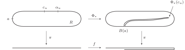
Figure 19. Schematic representation of $\Phi_{*}\colon R\to R$. The boundary of $R$ is identified with the circle $S$. The map $\Phi_{*}$ is injective except on $\gamma\setminus\{c_{u}\}=[\alpha_{u},a]\setminus\{c_{u}\}$, where it is two-to-one. We have $\Phi_{*}(a)=\Phi_{*}(\alpha_{u})=B(a)$, where $B$ is the outside map.

Definitions 5.28 ($\widehat{\Phi}_{*}\colon{\widehat{R}}\to{\widehat{R}}$, ${\widehat{\pi}}\colon{\widehat{R}}\to{\widehat{I}}$).

Write ${\widehat{R}}=\varprojlim(R,\Phi_{*})$, and let $\widehat{\Phi}_{*}\colon{\widehat{R}}\to{\widehat{R}}$ be the natural extension of $\Phi_{*}$. Let ${\widehat{\pi}}\colon{\widehat{R}}\to{\widehat{I}}$ be the function induced by the semi-conjugacy $\pi\colon R\to I$ of (P2), that is, ${\widehat{\pi}}({\boldsymbol{\xi}})_{i}=\pi(\xi_{i})$.

We will show (Theorem 5.31) that $F\colon\Sigma\to\Sigma$ is topologically conjugate to $\Phi\colon R/\!\!\sim\,\to R/\!\!\sim$. The proof is structured as follows. We first show (Lemma 5.29) that ${\widehat{\pi}}$ is a homeomorphism which conjugates $\widehat{\Phi}_{*}$ and ${\widehat{f}}$. There are therefore commutative diagrams

$$\begin{CD}{\widehat{R}}@>{\widehat{\Phi}_{*}}>{}>{\widehat{R}}\\ @V{{\widehat{\pi}}}V{}V@V{}V{{\widehat{\pi}}}V\\ {\widehat{I}}@>{{\widehat{f}}}>{}>{\widehat{I}}\\ @V{g}V{}V@V{}V{g}V\\ \Sigma @>{F}>{}>\Sigma\end{CD}\qquad\qquad\text{ and }\qquad\qquad\begin{CD}{\widehat{R}}@>{\widehat{\Phi}_{*}}>{}>{\widehat{R}}\\ @V{p_{0}}V{}V@V{}V{p_{0}}V\\ R@>{\Phi_{*}}>{}>R\\ @V{p_{\sim}}V{}V@V{}V{p_{\sim}}V\\ R/\!\sim @>{\Phi}>{}>R/\!\sim\end{CD}$$ (18)

where $p_{0}({\boldsymbol{\xi}})=\xi_{0}$, and $p_{\sim}$ is the canonical projection of $\sim$. In order to show that $F$ and $\Phi$ are conjugate, it therefore suffices to show that the fibers of $g\circ{\widehat{\pi}}$ agree with those of $p_{\sim}\circ p_{0}$: in other words, that $g({\widehat{\pi}}({\boldsymbol{\xi}}))=g({\widehat{\pi}}({\boldsymbol{\xi}}^{\prime}))$ if and only if $\xi_{0}\sim\xi_{0}^{\prime}$. This will be done using the description of the fibers of $g$ given in Remark 5.17, together with the technical Lemma 5.30.

Lemma 5.29.

${\widehat{\pi}}$ is a homeomorphism which conjugates $\widehat{\Phi}_{*}$ and ${\widehat{f}}$.

Proof.

${\widehat{\pi}}$ is clearly continuous, and semi-conjugates $\widehat{\Phi}_{*}$ and ${\widehat{f}}$ since $\pi$ semi-conjugates $\Phi_{*}$ and $f$. We will exhibit an explicit inverse $v\colon{\widehat{I}}\to{\widehat{R}}$ of ${\widehat{\pi}}$, which will establish the result since ${\widehat{R}}$ and ${\widehat{I}}$ are compact metric spaces.

To do this, we first define a function $h\colon{\widehat{I}}\to R$. Let ${\mathbf{x}}\in{\widehat{I}}$. Then ${\mathcal{F}}_{x_{0}}\supset\Phi_{*}({\mathcal{F}}_{x_{1}})\supset\Phi_{*}^{2}({\mathcal{F}}_{x_{2}})\supset\cdots$ by (P7) and (P8). Since each $\Phi_{*}^{j}({\mathcal{F}}_{x_{j}})$ is compact and non-empty by (P3) and (P1), the intersection $\bigcap_{j\geq 0}\Phi_{*}^{j}({\mathcal{F}}_{x_{j}})$ is non-empty; moreover, it contains a single point by (P5). We define $h({\mathbf{x}})\in{\mathcal{F}}_{x_{0}}$ to be the unique point of this intersection. Then $h\circ{\widehat{f}}=\Phi_{*}\circ h$ by construction. Moreover, $h$ is continuous: for if $U$ is a neighborhood of $h({\mathbf{x}})$, then by (P5) and the definition of $h$ there is some $N$ with $\Phi_{*}^{N}({\mathcal{F}}_{x_{N}})\subset U$. By (P4), if ${\mathbf{x}}^{\prime}$ is sufficiently close to ${\mathbf{x}}$ then we have also $\Phi_{*}^{N}({\mathcal{F}}_{x^{\prime}_{N}})\subset U$, and hence $h({\mathbf{x}}^{\prime})\in U$.

Define $v\colon{\widehat{I}}\to{\widehat{R}}$ by $v({\mathbf{x}})_{i}=h({\widehat{f}}^{-i}({\mathbf{x}}))$. That $v({\mathbf{x}})\in{\widehat{R}}$ follows from $\Phi_{*}\circ h=h\circ{\widehat{f}}$, which gives $\Phi_{*}(h({\widehat{f}}^{-(i+1)}({\mathbf{x}})))=h({\widehat{f}}^{-i}({\mathbf{x}}))$ for each $i$.

We now show that $v$ is inverse to ${\widehat{\pi}}$. First, let ${\mathbf{x}}\in{\widehat{I}}$. Then for each $i\geq 0$,

$${\widehat{\pi}}(v({\mathbf{x}}))_{i}=\pi(v({\mathbf{x}})_{i})=\pi(h({\widehat{f}}^{-i}({\mathbf{x}})))=x_{i},$$

since $h({\widehat{f}}^{-i}({\mathbf{x}}))=h(\left<x_{i},x_{i+1},\ldots\right>)\in{\mathcal{F}}_{x_{i}}$. On the other hand, if ${\boldsymbol{\xi}}\in{\widehat{R}}$, then for each $i\geq 0$,

$$v({\widehat{\pi}}({\boldsymbol{\xi}}))_{i}=h({\widehat{f}}^{-i}({\widehat{\pi}}({\boldsymbol{\xi}})))=h(\left<\pi(\xi_{i}),\pi(\xi_{i+1}),\ldots\right>)=\xi_{i},$$

since for every $j\geq 0$ we have $\xi_{i}=\Phi_{*}^{j}(\xi_{i+j})\in\Phi_{*}^{j}({\mathcal{F}}_{\pi(\xi_{i+j})})$, so that $\xi_{i}$ is the unique element of $\bigcap_{j\geq 0}\Phi_{*}^{j}({\mathcal{F}}_{\pi(\xi_{i+j})})$. ∎

The following lemma expresses the connection between the equivalence relation $\sim$ defined in (P9) and the identifications on ${\widehat{I}}$ described in Remark 5.17.

Lemma 5.30.

Let ${\boldsymbol{\xi}},{\boldsymbol{\xi}}^{\prime}\in{\widehat{R}}$.

1. If $f$ is of rational general type, then $\xi_{0}=\xi_{0}^{\prime}$ but $\xi_{1}\not=\xi_{1}^{\prime}$ if and only if either

   $$\{{\widehat{\pi}}({\boldsymbol{\xi}}),\,{\widehat{\pi}}({\boldsymbol{\xi}}^{\prime})\} = \{\omega({\mathbf{t}}(y,0,0)),\,\omega({\mathbf{t}}({\widehat{y}},0,0))\}\text{ for some }y\in\gamma\setminus\{c_{u},q_{n-1},{\widehat{q}}_{n-1}\};\text{ or}$$

   $$\{{\widehat{\pi}}({\boldsymbol{\xi}}),\,{\widehat{\pi}}({\boldsymbol{\xi}}^{\prime})\} = \{\omega({\mathbf{t}}({\widehat{q}}_{n-1},0,0)),\,\omega({\mathbf{t}}(a,1,0))\};\text{ or}$$

   $$\{{\widehat{\pi}}({\boldsymbol{\xi}}),\,{\widehat{\pi}}({\boldsymbol{\xi}}^{\prime})\} = \{\omega({\mathbf{t}}({\widehat{q}}_{n-1},0,0)),\,\omega({\mathbf{t}}(\alpha_{u},1,0))\}.$$

2. If $f$ is of rational NBT type, then $\xi_{0}=\xi_{0}^{\prime}$ but $\xi_{1}\not=\xi_{1}^{\prime}$ if and only if

   $$\{{\widehat{\pi}}({\boldsymbol{\xi}}),\,{\widehat{\pi}}({\boldsymbol{\xi}}^{\prime})\}=\{\omega({\mathbf{t}}(y,0,0)),\,\omega({\mathbf{t}}({\widehat{y}},0,0))\}\text{ for some }y\in\gamma\setminus\{c_{u}\}.$$

3. If $f$ is of rational (normal) endpoint type, then $\xi_{0}=\xi_{0}^{\prime}$ but $\xi_{1}\not=\xi_{1}^{\prime}$ if and only if either

   $$\{{\widehat{\pi}}({\boldsymbol{\xi}}),\,{\widehat{\pi}}({\boldsymbol{\xi}}^{\prime})\} = \{\omega({\mathbf{t}}(y,0,0)),\,\omega({\mathbf{t}}({\widehat{y}},0,0))\}\text{ for some }y\in{{\accentset{\circ}{\gamma}}}\setminus\{c_{u}\};\text{ or}$$

   $$\{{\widehat{\pi}}({\boldsymbol{\xi}}),\,{\widehat{\pi}}({\boldsymbol{\xi}}^{\prime})\} = \{\omega({\mathbf{t}}(A,0,0)),\,\omega({\mathbf{t}}(A,\ell,0))\}\text{ for some }\ell>0;\text{ or}$$

   $$\{{\widehat{\pi}}({\boldsymbol{\xi}}),\,{\widehat{\pi}}({\boldsymbol{\xi}}^{\prime})\} = \{\omega({\mathbf{t}}(A,0,0)),\,\omega({\mathbf{q}}_{0})\},$$

   where $A=a$ if $\kappa(f)=\operatorname{rhe}(m/n)$, and $A=\alpha_{u}$ if $\kappa(f)=\operatorname{lhe}(m/n)$.

4. If $f$ is of rational (normal) endpoint type, then there is some $r\geq 0$ with $\Phi_{*}^{r}(\xi_{0})\in P$ (the periodic orbit of (P9)) if and only if there is some $i$ with $0\leq i\leq n-1$ such that either ${\widehat{\pi}}({\boldsymbol{\xi}})=\omega({\mathbf{q}}_{i})$, or ${\widehat{\pi}}({\boldsymbol{\xi}})=\omega({\mathbf{t}}(A,k,i))$ for some $k\in{\mathbb{Z}}$, where $A=a$ if $\kappa(f)=\operatorname{rhe}(m/n)$, and $A=\alpha_{u}$ if $\kappa(f)=\operatorname{lhe}(m/n)$.

Proof.

Assume first that $f$ is of general type. By (P10), we have $\xi_{0}=\xi_{0}^{\prime}$ but $\xi_{1}\not=\xi_{1}^{\prime}$ if and only if $\{\xi_{1},\xi_{1}^{\prime}\}=\{y,{\widehat{y}}\}$ for some $y\in\gamma\setminus\{c_{u}\}$.

Since (i) $\Phi_{*}^{-1}(\partial R)\subset\partial R$; (ii) the only point of $\partial R$ which has more than one preimage is $q_{0}=\Phi_{*}(a)=\Phi_{*}(\alpha_{u})$; and (iii) the only point of $\gamma$ on the orbit of $q_{0}$ is $q_{n-1}$, it follows that, for $y\in\gamma\setminus\{c_{u},q_{n-1},{\widehat{q}}_{n-1}\}$, we have

$$\{\xi_{1},\,\xi_{1}^{\prime}\}=\{y,\,{\widehat{y}}\} \iff \{{\boldsymbol{\xi}},\,{\boldsymbol{\xi}}^{\prime}\}=\{\left<\Phi_{*}(y),y,B^{-1}(y),\ldots\right>,\,\left<\Phi_{*}(y),{\widehat{y}},B^{-1}({\widehat{y}}),\ldots\right>\}$$

$$\iff \{{\widehat{\pi}}({\boldsymbol{\xi}}),\,{\widehat{\pi}}({\boldsymbol{\xi}}^{\prime})\}=\{\left<f(\tau(y)),\tau(y),\tau(B^{-1}(y)),\ldots\right>,\,\left<f(\tau(y)),\tau({\widehat{y}}),\tau(B^{-1}({\widehat{y}})),\ldots\right>\}$$

$$\iff \{{\widehat{\pi}}({\boldsymbol{\xi}}),\,{\widehat{\pi}}({\boldsymbol{\xi}}^{\prime})\}=\{\omega({\mathbf{t}}(y,0,0)),\,\omega({\mathbf{t}}({\widehat{y}},0,0))\}.$$

Here we have used (P6) (in particular that $\Phi_{*}=B$ on $S\setminus{{\accentset{\circ}{\gamma}}}$ in the first line, and that $\pi=\tau$ on $S$ in the second line); we have used that $\pi\circ\Phi_{*}=f\circ\pi$ in the second line; and we have used (17) in the final line.

In the case $y\in\{q_{n-1},{\widehat{q}}_{n-1}\}$, we have $\xi_{1}=q_{n-1}$ if and only if

$${\boldsymbol{\xi}}=\left<\Phi_{*}(q_{n-1}),q_{n-1},q_{n-2},\ldots,q_{0},a,B^{-1}(a),\ldots\right>\text{ or }{\boldsymbol{\xi}}=\left<\Phi_{*}(q_{n-1}),q_{n-1},q_{n-2},\ldots,q_{0},\alpha_{u},B^{-1}(\alpha_{u}),\ldots\right>;$$

while $\xi_{1}={\widehat{q}}_{n-1}$ if and only if ${\boldsymbol{\xi}}=\left<\Phi_{*}({\widehat{q}}_{n-1}),{\widehat{q}}_{n-1},B^{-1}({\widehat{q}}_{n-1}),\ldots\right>$. These give the other two possibilities in the statement of (a), using (17).

The argument in the NBT case is identical, except that the case $y\in\{q_{n-1},{\widehat{q}}_{n-1}\}$ does not arise since $q_{n-1}=c_{u}$.

Suppose then that $f$ is of normal endpoint type. As in the general case, we have $\xi_{0}=\xi_{0}^{\prime}$ but $\xi_{1}\not=\xi_{1}^{\prime}$ if and only if $\{\xi_{1},\,\xi_{1}^{\prime}\}=\{y,\,{\widehat{y}}\}$ for some $y\in\gamma\setminus\{c_{u}\}$. The argument for $y\not\in\{c_{u},q_{n-1},{\widehat{q}}_{n-1}\}$ (i.e. for $y\in{{\accentset{\circ}{\gamma}}}\setminus\{c_{u}\}$) is identical to the general case. Suppose then, without loss of generality, that $\xi_{1}=a$ and $\xi_{1}^{\prime}=\alpha_{u}$.

Consider first the case where $\kappa(f)=\operatorname{rhe}(m/n)$, so that we have $B^{n}(a)=B^{n}(\alpha_{u})=\alpha_{u}$. Then

$${\boldsymbol{\xi}}=\left<q_{0},a,B^{-1}(a),\ldots\right>,$$

while either

$${\boldsymbol{\xi}}^{\prime}=\left<(q_{0},\alpha_{u},q_{n-2},\ldots,q_{1})^{\infty}\right>\quad\text{ or }\quad{\boldsymbol{\xi}}^{\prime}=\left<(q_{0},\alpha_{u},q_{n-2},\ldots,q_{1})^{\ell},q_{0},a,B^{-1}(a),\ldots\right>\text{ for some }\ell>0.$$

Therefore ${\widehat{\pi}}({\boldsymbol{\xi}})=\omega({\mathbf{t}}(a,0,0))$; while either ${\widehat{\pi}}({\boldsymbol{\xi}}^{\prime})=\omega({\mathbf{q}}_{i})$ or ${\widehat{\pi}}({\boldsymbol{\xi}}^{\prime})=\omega({\mathbf{t}}(a,\ell,0))$ for some $\ell>0$. Here we have used (17); and we have used (10) to show that ${\widehat{\pi}}(\left<(q_{0},\alpha_{u},q_{n-2},\ldots,q_{1})^{\infty}\right>)=\omega({\mathbf{q}}_{i})$.

The case where $\kappa(f)=\operatorname{lhe}(m/n)$ works analogously, and the result follows.

For (d), there is some $r\geq 0$ with $\Phi_{*}^{r}(\xi_{0})\in P$ if and only if either $\xi_{0}\in P$ (i.e. $\xi_{0}=q_{i}$ for some $i$), or $\xi_{0}=B^{-s}(A)$ for some $s\geq 0$. This is equivalent to

$${\boldsymbol{\xi}} = \left<(q_{i},q_{i-1},\ldots,q_{0},q_{n-1},\ldots,q_{i+1})^{\infty}\right>\quad\text{ for some~{}$i$, or}$$

$${\boldsymbol{\xi}} = \left<q_{i},q_{i-1},\ldots,q_{0},(q_{n-1},\ldots,q_{0})^{k},A,B^{-1}(A),\ldots\right>\quad\text{ for some~{}$i$ and some $k\geq 0$, or}$$

$${\boldsymbol{\xi}} = \left<B^{-s}(A),B^{-(s+1)}(A),\ldots\right>\quad\text{ for some $s\geq 0$}.$$

The first of these is equivalent to ${\widehat{\pi}}({\boldsymbol{\xi}})=\omega({\mathbf{q}}_{i})$ for some $i$; the second to ${\widehat{\pi}}({\boldsymbol{\xi}})=\omega({\mathbf{t}}(A,k,i))$ for some $i$ and some $k\geq 0$; and the third (noting Remark 4.51) to ${\widehat{\pi}}({\boldsymbol{\xi}})=\omega({\mathbf{t}}(A,k,i))$ for some $i$ and some $k<0$. ∎

Theorem 5.31.

Let $f$ be a post-critically finite tent map of slope $t>\sqrt{2}$. Then the sphere homeomorphism $F\colon\Sigma\to\Sigma$ constructed in the proof of Theorem 5.15 is topologically conjugate to the generalized pseudo-Anosov $\Phi\colon R/\!\!\sim\,\to\,R/\!\!\sim$ constructed in [21].

Proof.

By (18) and the accompanying discussion, it is only necessary to show that for all pairs ${\boldsymbol{\xi}},{\boldsymbol{\xi}}^{\prime}$ of distinct elements of ${\widehat{R}}$, we have $g({\widehat{\pi}}({\boldsymbol{\xi}}))=g({\widehat{\pi}}({\boldsymbol{\xi}}^{\prime}))$ if and only if $\xi_{0}\sim\xi_{0}^{\prime}$.

We start with the case where $f$ is of general type. In this case the points of $P$ (the periodic orbit of (P9)) have unique $\Phi_{*}$-preimages — which are, of course, in  $P$ — and hence, by (P9), $\xi_{0}\sim\xi_{0}^{\prime}$ if and only if either

1. $\Phi_{*}^{r}(\xi_{0})=\Phi_{*}^{r}(\xi^{\prime}_{0})$ for some $r\geq 0$; or

2. $\xi_{0},\xi^{\prime}_{0}\in P$.

Since ${\boldsymbol{\xi}}\not={\boldsymbol{\xi}}^{\prime}$, condition (i) is equivalent to the condition

$$\text{There is some }s\in{\mathbb{Z}}\text{ with }\quad\widehat{\Phi}_{*}^{s}({\boldsymbol{\xi}})_{0}=\widehat{\Phi}_{*}^{s}({\boldsymbol{\xi}}^{\prime})_{0},\quad\text{ but }\quad\widehat{\Phi}_{*}^{s}({\boldsymbol{\xi}})_{1}\not=\widehat{\Phi}_{*}^{s}({\boldsymbol{\xi}}^{\prime})_{1}.$$ (19)

For if (19) holds, then either $s\leq 0$, in which case $\xi_{0}=\xi_{0}^{\prime}$; or $s>0$, in which case $\Phi_{*}^{r}(\xi_{0})=\Phi_{*}^{r}(\xi^{\prime}_{0})$ for $r=s$. Conversely, suppose that there is some $r\geq 0$ for which $\Phi_{*}^{r}(\xi_{0})=\Phi_{*}^{r}(\xi_{0}^{\prime})$, and pick this $r$ to be as small as possible. If $r>0$ then we have $\widehat{\Phi}_{*}^{r}({\boldsymbol{\xi}})_{0}=\widehat{\Phi}_{*}^{r}({\boldsymbol{\xi}}^{\prime})_{0}$, but $\Phi_{*}^{r-1}(\xi_{0})\not=\Phi_{*}^{r-1}(\xi_{0}^{\prime})$, so that $\widehat{\Phi}_{*}^{r-1}({\boldsymbol{\xi}})_{0}\not=\widehat{\Phi}_{*}^{r-1}({\boldsymbol{\xi}}^{\prime})_{0}$; that is, $\widehat{\Phi}_{*}^{r}({\boldsymbol{\xi}})_{1}\not=\widehat{\Phi}_{*}^{r}({\boldsymbol{\xi}}^{\prime})_{1}$, and hence (19) holds with $s=r$. On the other hand, if $r=0$ then $\xi_{0}=\xi^{\prime}_{0}$. Since ${\boldsymbol{\xi}}\not={\boldsymbol{\xi}}^{\prime}$, there is some greatest $i\geq 0$ with $\xi_{i}=\xi^{\prime}_{i}$. Then we have $\widehat{\Phi}_{*}^{-i}({\boldsymbol{\xi}})_{0}=\widehat{\Phi}_{*}^{-i}({\boldsymbol{\xi}}^{\prime})_{0}$ but $\widehat{\Phi}_{*}^{-i}({\boldsymbol{\xi}})_{1}\not=\widehat{\Phi}_{*}^{-i}({\boldsymbol{\xi}}^{\prime})_{1}$, so that (19) holds with $s=-i$.

Therefore condition (i) holds if and only if there is some $s\in{\mathbb{Z}}$ such that $\{{\widehat{\pi}}(\widehat{\Phi}_{*}^{s}({\boldsymbol{\xi}})),\,{\widehat{\pi}}(\widehat{\Phi}_{*}^{s}({\boldsymbol{\xi}}^{\prime}))\}$ is one of the pairs from the statement of Lemma 5.30 (a). By Lemma 5.29, this is equivalent to the existence of $s\in{\mathbb{Z}}$ such that $\{{\widehat{f}}^{s}({\widehat{\pi}}({\boldsymbol{\xi}})),\,{\widehat{f}}^{s}({\widehat{\pi}}({\boldsymbol{\xi}}^{\prime}))\}$ is one of these pairs. Setting $r=-s$, this in turn is equivalent to the existence of $r\in{\mathbb{Z}}$ such that $\{{\widehat{\pi}}({\boldsymbol{\xi}}),\,{\widehat{\pi}}({\boldsymbol{\xi}}^{\prime})\}$ is the image under ${\widehat{f}}^{r}$ of one of these pairs. That is, condition (i) holds if and only if there is some $k\in{\mathbb{Z}}$ and $0\leq i\leq n-1$ such that

$$\{{\widehat{\pi}}({\boldsymbol{\xi}}),\,{\widehat{\pi}}({\boldsymbol{\xi}}^{\prime})\} = \{\omega({\mathbf{t}}(y,k,i)),\,\omega({\mathbf{t}}({\widehat{y}},k,i))\}\text{ for some }y\in\gamma\setminus\{c_{u},q_{n-1},{\widehat{q}}_{n-1}\};\text{ or}$$

$$\{{\widehat{\pi}}({\boldsymbol{\xi}}),\,{\widehat{\pi}}({\boldsymbol{\xi}}^{\prime})\} = \{\omega({\mathbf{t}}({\widehat{q}}_{n-1},k,i),\,\omega({\mathbf{t}}(a,k+1,i))\};\text{ or}$$

$$\{{\widehat{\pi}}({\boldsymbol{\xi}}),\,{\widehat{\pi}}({\boldsymbol{\xi}}^{\prime})\} = \{\omega({\mathbf{t}}({\widehat{q}}_{n-1},k,i),\,\omega({\mathbf{t}}(\alpha_{u},k+1,i))\}.$$

Observing that condition (ii) holds if and only if ${\widehat{\pi}}({\boldsymbol{\xi}}),{\widehat{\pi}}({\boldsymbol{\xi}}^{\prime})\in\omega({\mathbf{P}})$ and comparing with Remark 5.17 (e), we see that $\xi_{0}\sim\xi_{0}^{\prime}$ if and only if $g({\widehat{\pi}}({\boldsymbol{\xi}}))=g({\widehat{\pi}}({\boldsymbol{\xi}}^{\prime}))$.

The proof in the NBT case is similar, using Lemma 5.30 (b) and Remark 5.17 (f).

Suppose, then, than $f$ is of (normal) endpoint type, so that $q_{n-1}$ is either $a$ or $\alpha_{u}$: as before, we will write $A={\widehat{q}}_{n-1}$, so that $q_{n-1}=\alpha_{u}$ and $A=a$ when $\kappa(f)=\operatorname{rhe}(m/n)$; while $q_{n-1}=a$ and $A=\alpha_{u}$ when $\kappa(f)=\operatorname{lhe}(m/n)$. The periodic orbit $P$ of $\Phi_{*}$ on $\partial R$ is therefore $P=\{q_{0},q_{1},\ldots,q_{n-1}\}$ (that is, it is equal to $Q$), and the two $\Phi_{*}$-preimages of $q_{0}$ are $a$ and $\alpha_{u}$. By (P9), $\xi_{0}\sim\xi_{0}^{\prime}$ if and only if either

1. $\Phi_{*}^{r}(\xi_{0})=\Phi_{*}^{r}(\xi_{0}^{\prime})$ for some $r\geq 0$; or

2. $\Phi_{*}^{r}(\xi_{0}),\Phi_{*}^{r}(\xi_{0}^{\prime})\in P$ for some $r\geq 0$.

As in the general case, condition (i) is equivalent to (19), which in turn is equivalent to the existence of $r\in{\mathbb{Z}}$ such that $\{{\widehat{\pi}}({\boldsymbol{\xi}}),{\widehat{\pi}}({\boldsymbol{\xi}}^{\prime})\}$ is the image under ${\widehat{f}}^{r}$ of one of the pairs from the statement of Lemma 5.30 (c). That is, condition (i) holds if and only if there is some $k\in{\mathbb{Z}}$ and $0\leq i\leq n-1$ such that

$$\{{\widehat{\pi}}({\boldsymbol{\xi}}),\,{\widehat{\pi}}({\boldsymbol{\xi}}^{\prime})\} = \{\omega({\mathbf{t}}(y,k,i)),\,\omega({\mathbf{t}}({\widehat{y}},k,i))\}\text{ for some }y\in{{\accentset{\circ}{\gamma}}}\setminus\{c_{u}\};\text{ or}$$

$$\{{\widehat{\pi}}({\boldsymbol{\xi}}),\,{\widehat{\pi}}({\boldsymbol{\xi}}^{\prime})\} = \{\omega({\mathbf{t}}(A,k,i),\,\omega({\mathbf{t}}(A,k+\ell,i))\}\text{ for some }\ell>0;\text{ or}$$

$$\{{\widehat{\pi}}({\boldsymbol{\xi}}),\,{\widehat{\pi}}({\boldsymbol{\xi}}^{\prime})\} = \{\omega({\mathbf{t}}(A,k,i),\,\omega({\mathbf{q}}_{i})\}.$$

On the other hand, by Lemma 5.30 (d), condition (ii) holds if and only if there are integers $k$ and $k^{\prime}$, and $0\leq i,i^{\prime}\leq n-1$ such that ${\widehat{\pi}}({\boldsymbol{\xi}})=\omega({\mathbf{q}}_{i})$ or ${\widehat{\pi}}({\boldsymbol{\xi}})=\omega({\mathbf{t}}(A,k,i))$; and ${\widehat{\pi}}({\boldsymbol{\xi}}^{\prime})=\omega({\mathbf{q}}_{i^{\prime}})$ or ${\widehat{\pi}}({\boldsymbol{\xi}}^{\prime})=\omega({\mathbf{t}}(A,k^{\prime},i^{\prime}))$.

Combining conditions (i) and (ii), we obtain that $\xi_{0}\sim\xi_{0}^{\prime}$ if and only if either there exist $y\in{{\accentset{\circ}{\gamma}}}\setminus\{c_{u}\}$, $k\in{\mathbb{Z}}$, and $0\leq i\leq n-1$ such that $\{{\widehat{\pi}}({\boldsymbol{\xi}}),\,{\widehat{\pi}}({\boldsymbol{\xi}}^{\prime})\}=\{\omega({\mathbf{t}}(y,k,i)),\,\omega({\mathbf{t}}({\widehat{y}},k,i))\}$; or

$$\{{\widehat{\pi}}({\boldsymbol{\xi}}),\,{\widehat{\pi}}({\boldsymbol{\xi}}^{\prime})\}\subset\omega({\mathbf{Q}})\cup\{\omega({\mathbf{t}}(A,k,i))\,:\,k\in{\mathbb{Z}},\,0\leq i\leq n-1\}.$$

Comparing with Remark 5.17 (c), we see that $\xi_{0}\sim\xi_{0}^{\prime}$ if and only if $g({\widehat{\pi}}({\boldsymbol{\xi}}))=g({\widehat{\pi}}({\boldsymbol{\xi}}^{\prime}))$, as required. ∎

A detailed description of the dynamics of the sphere homeomorphism $F$ in the case where $f$ is a tent map but is not post-critically finite is the subject of ongoing research. Here we only give a straightforward statement about the way in which dynamical properties of a general $f$ carry over to $F$. Recall that a Borel probability measure on a topological manifold $M$ is called an Oxtoby-Ulam measure, or OU-measure, if it is non-atomic, positive on open sets, and assigns zero measure to the boundary of $M$ (if it has one).

Theorem 5.32 (Sphere homeomorphism dynamics).

Let $f$ be a unimodal map satisfying the conditions of Convention 2.8, and $F\colon\Sigma\to\Sigma$ be the corresponding sphere homeomorphism given by Theorem 5.15. Then

1. if $f$ is topologically transitive then so is $F$;

2. if $f$ has dense periodic points, then so does $F$;

3. $f$ and $F$ have the same number of periodic orbits of each period, with the exception that, provided $\kappa(f)\not=10^{\infty}$,

   • $F$ has one more fixed point than $f$, and

   • if $f$ is of rational type with $q(\kappa(f))=m/n\in(0,1/2)$, then $F$ has either one or two fewer period $n$ orbits than $f$.

4. $f$ and $F$ have the same topological entropy; and

5. if $f$ preserves an ergodic OU-measure, then $F$ preserves an ergodic OU-measure with the same metric entropy.

In particular, if $f$ is a tent map of slope $t\in(\sqrt{2},2]$ restricted to its dynamical interval, then $F$ is topologically transitive, has dense periodic points, has topological entropy $\log(t)$, and has an invariant ergodic OU-measure with metric entropy $\log(t)$.

Proof.

It is well known that if $f$ is topologically transitive or has dense periodic points, then the same is true of its natural extension ${\widehat{f}}$. Since these properties are preserved by semi-conjugacy, (a) and (b) follow.

(c) follows from the explicit descriptions of the fibers of the semi-conjugacy $g\colon{\widehat{I}}\to\Sigma$ given in Remark 5.17. The only fiber which contains periodic points is the exceptional fiber in the rational case: in the normal endpoint case this fiber contains the period $n$ orbit $\omega({\mathbf{Q}})$; in the interior and late endpoint cases it is equal to the period $n$ orbit $\omega({\mathbf{P}})$; and in the early or quadratic-like strict endpoint cases, it contains both period $n$ orbits $\omega({\mathbf{P}})$ and $\omega({\mathbf{Q}})$ (or the single semi-stable orbit $\omega({\mathbf{P}})=\omega({\mathbf{Q}})$). In all cases, the exceptional fiber is collapsed to a fixed point of $F$.

(d) is established in Remark 5.16.

For (e), it is also well known that if $\mu$ is an $f$-invariant Borel probability measure, then there is a unique ${\widehat{f}}$-invariant Borel probability measure ${\widehat{\mu}}$ on ${\widehat{I}}$ characterized by $(\pi_{n})_{*}({\widehat{\mu}})=\mu$ for all $n$ (here $\pi_{n}\colon{\widehat{I}}\to I$ is defined by $\pi_{n}({\mathbf{x}})=x_{n}$); moreover, ${\widehat{\mu}}$ is ergodic if and only if $\mu$ is; and $\mu$ and ${\widehat{\mu}}$ have the same metric entropy. If ${\widehat{\mu}}$ were atomic then $\mu$ would be also. Moreover, since a base for the topology on ${\widehat{I}}$ is given by the set of all $\pi_{n}^{-1}(U)$, where $U$ is non-empty and open in $I$, and since ${\widehat{\mu}}(\pi_{n}^{-1}(U))=\mu(U)$, we have that ${\widehat{\mu}}$ is positive on open sets if $\mu$ is.

Write ${\tilde{\mu}}=g_{*}({\widehat{\mu}})$, so that ${\tilde{\mu}}$ is $F$-invariant and ergodic. Since $g$ is continuous, ${\tilde{\mu}}$ is also positive on open sets. To show that ${\tilde{\mu}}$ is non-atomic, suppose for a contradiction that there were some $z\in\Sigma$ with ${\tilde{\mu}}(z)>0$. Then, since ${\tilde{\mu}}$ is $F$-invariant and ergodic, $z$ would belong to a periodic orbit of full measure, a contradiction since the complement of this periodic orbit would be open and non-empty.

Except perhaps for a single point (which we now know has ${\tilde{\mu}}$-measure zero), the point preimages of the semi-conjugacy $g$ are finite. Thus $g$ has finite preimages ${\tilde{\mu}}$-almost everywhere and so ${\widehat{\mu}}$ and ${\tilde{\mu}}$ have the same metric entropy.

Therefore ${\tilde{\mu}}$ is an $F$-invariant ergodic OU-measure as required. Since tent maps of slope $t>\sqrt{2}$ restricted to their dynamical intervals are transitive, have dense periodic points, have topological entropy $\log(t)$, and have invariant ergodic OU-measures with metric entropy $\log(t)$, the final statement follows. ∎

Remark 5.33.

A theorem of Oxtoby and Ulam (see [35] and Appendix 2 of [3]) states that if $m_{1}$ and $m_{2}$ are OU-measures on a manifold $M$, then there is a homeomorphism $h\colon M\to M$ with $h_{*}(m_{1})=m_{2}$. Therefore by conjugating the sphere homeomorphism $F$, we can make it preserve any OU-measure; in particular, one coming from an area form on $\Sigma$.

Appendix A The embedding is independent of the unwrapping

In this appendix we will prove the following result, which establishes that the prime ends of $({\widehat{T}},{\widehat{I}})$ are independent of the choice of unwrapping of the unimodal map $f$.

Theorem 2.15. Any two unwrappings of a unimodal map $f$ are equivalent.

Recall that unwrappings $\overline{f}_{0}$ and $\overline{f}_{1}$ of $f$, which have associated Barge-Martin homeomorphisms ${\widehat{H}}_{0}\colon({\widehat{T}}_{0},{\widehat{I}})\to({\widehat{T}}_{0},{\widehat{I}})$ and ${\widehat{H}}_{1}\colon({\widehat{T}}_{1},{\widehat{I}})\to({\widehat{T}}_{1},{\widehat{I}})$, are equivalent if there is a homeomorphism $\lambda\colon{\widehat{T}}_{0}\to{\widehat{T}}_{1}$ which restricts to the identity on ${\widehat{I}}$. Theorem 2.15 is a consequence of the following recent deep result (Theorem 7.3 of [34]).

Theorem A.1 (Oversteegen–Tymchatyn).

Let $K$ be a continuum and $\{\alpha_{t}\}_{t\in[0,1]}\colon K\to S^{2}$ be an isotopy of embeddings of $K$ into the sphere. Then there is an ambient isotopy $\{A_{t}\}_{t\in[0,1]}\colon S^{2}\to S^{2}$ with $A_{0}=\operatorname{id}$ and $\alpha_{t}=A_{t}\circ\alpha_{0}$ for all $t$.

Definition A.2 (Weak unwrapping).

A weak unwrapping of a unimodal map $f$ is an orientation-preserving near-homeomorphism $\overline{f}\colon T\to T$ which is injective on $I$ with $\overline{f}(I)\subset\{(y,s)\,:\,s\geq 1/2\}$, and satisfies $\Upsilon\circ\overline{f}|_{I}=f$.

Remark A.3.

A weak unwrapping differs from an unwrapping in that it is not required that the second component of $\overline{f}(y,s)$ is equal to $s$ whenever $s\in[0,1/2]$. A Barge-Martin homeomorphism can be associated to a weak unwrapping in exactly the same way as to an unwrapping, although it may not have ${\widehat{I}}$ as a global attractor (if $\overline{f}$ pushes points with $s\in[0,1/2]$ outwards more strongly than the smash $\Upsilon$ pulls them inwards).

Definition A.4 (u-near-isotopy).

A homotopy $\{\overline{f}_{t}\}\colon T\to T$ of weak unwrappings of a fixed unimodal map $f$ is called a u-near-isotopy (for “unwrapping near-isotopy”).

Remark A.5.

It is not obvious that a homotopy of near-homeomorphisms of $T$ can be uniformly approximated by isotopies, and therefore merits the name near-isotopy. That this is the case follows from a theorem of Edwards and Kirby (Corollary 1.1 of [24]), which states that the homeomorphism group of any manifold is locally contractible, and hence locally path connected.

Lemma A.6.

Any two u-near-isotopic unwrappings $\overline{f}_{0}\colon T\to T$ and $\overline{f}_{1}\colon T\to T$ of a unimodal map $f$ are equivalent.

Proof.

Let $\{\overline{f}_{t}\}$ be a u-near isotopy from $\overline{f}_{0}$ to $\overline{f}_{1}$, and for each $t$ let ${\widehat{H}}_{t}\colon({\widehat{T}}_{t},{\widehat{I}})\to({\widehat{T}}_{t},{\widehat{I}})$ be the Barge-Martin homeomorphism associated with $\overline{f}_{t}$. By Theorem 2.14, there are homeomorphisms $h_{t}\colon{\widehat{T}}_{t}\to S^{2}$ with the property that $\{\Phi_{t}=h_{t}\circ{\widehat{H}}_{t}\circ h_{t}^{-1}\}\colon S^{2}\to S^{2}$ is an isotopy. It follows from the construction of the homeomorphisms $h_{t}$ (as compositions $h_{t}=p_{1}\circ\beta\circ\iota_{t}$) in the proof of Corollary 2.3 of [14] — which applies equally well to weak unwrappings as to unwrappings — that $h_{t}|_{{\widehat{I}}}$ varies continuously with $t$, so that $\{h_{t}|_{\widehat{I}}\}$ is an isotopy of embeddings of the continuum ${\widehat{I}}$ into $S^{2}$.

By Theorem A.1, there is an isotopy $\{A_{t}\}\colon S^{2}\to S^{2}$ with $A_{0}=\operatorname{id}$ and $h_{t}|_{{\widehat{I}}}=A_{t}\circ h_{0}|_{{\widehat{I}}}$ for all $t$. Let $\lambda=h_{1}^{-1}\circ A_{1}\circ h_{0}\colon{\widehat{T}}_{0}\to{\widehat{T}}_{1}$. Then $\lambda$ is the required homeomorphism which restricts to the identity on ${\widehat{I}}$. ∎

Remark A.7.

Lemma A.6 extends to apply to any continuous surjection $f\colon K\to K$, where $K$ is a Peano non-separating planar continuum. A theorem of Brechner and Brown [15] states that such a continuum $K$ has a Disk Mapping Cylinder Neighborhood: that is, it can be embedded in a disk $D$ in such a way that there is a continuous map $\phi\colon S^{1}\times[0,1]\to D$ with $K=\phi(S^{1}\times\{1\})$, and $\phi(y_{1},s_{1})=\phi(y_{2},s_{2})\implies s_{1}=s_{2}=1$. (In fact, Brechner and Brown show that a planar continuum has a Disk Mapping Cylinder Neighborhood if and only if it is Peano and non-separating.) Using the associated “coordinates” $(y,s)$, the Barge-Martin construction can be carried out exactly as in the case $K=I$, and the proof of Lemma A.6 goes through without change.

We next show that there are only two u-near-isotopy classes of unwrappings of a given unimodal map $f$. Since a weak unwrapping $\overline{f}$ is injective on $I$, one of the following two cases must occur

1. For every $x\in[a,c)$ either $\overline{f}(x)=(f(x)_{u},s_{1})$ and $\overline{f}({\hat{x}})=(f(x)_{\ell},s_{2})$; or $\overline{f}(x)=(f(x)_{u},s_{1})$ and $\overline{f}({\hat{x}})=(f(x)_{u},s_{2})$ with $s_{1}<s_{2}$; or $\overline{f}(x)=(f(x)_{\ell},s_{1})$ and $\overline{f}({\hat{x}})=(f(x)_{\ell},s_{2})$ with $s_{1}>s_{2}$.

2. For every $x\in[a,c)$ either $\overline{f}(x)=(f(x)_{\ell},s_{1})$ and $\overline{f}({\hat{x}})=(f(x)_{u},s_{2})$; or $\overline{f}(x)=(f(x)_{u},s_{1})$ and $\overline{f}({\hat{x}})=(f(x)_{u},s_{2})$ with $s_{1}>s_{2}$; or $\overline{f}(x)=(f(x)_{\ell},s_{1})$ and $\overline{f}({\hat{x}})=(f(x)_{\ell},s_{2})$ with $s_{1}<s_{2}$.

We say that $\overline{f}$ is of type “up” in case (a), and of type “down” in case (b) (our preferred unwrapping is therefore of type “down”).

Lemma A.8.

If two unwrappings $\overline{f}_{0}$ and $\overline{f}_{1}$ of a unimodal map $f$ are of the same type, then they are u-near-isotopic.

Proof.

We show first that any unwrapping $\overline{f}$ of $f$ is u-near-isotopic to a weak unwrapping which is a homeomorphism, and which has the same type as $\overline{f}$. Since $\overline{f}$ is a near-homeomorphism, it follows from the theorem of Edwards and Kirby stated in Remark A.5 that it is the endpoint of a pseudo-isotopy: that is, that there is a homotopy $\{g_{t}\}\colon T\to T$ with $g_{0}=\overline{f}$ and $g_{t}$ a homeomorphism for $t>0$. Define $\alpha_{t}=g_{t}|_{I}\colon I\to T$. Since $\overline{f}|_{I}$ is a homeomorphism by definition, $\{\alpha_{t}\}$ is an isotopy of embeddings. By Theorem A.1, there is an isotopy $\{A_{t}\}\colon T\to T$ with $A_{0}=\operatorname{id}$ and $\alpha_{t}=A_{t}\circ\alpha_{0}$ for all $t$. Define $\overline{g}_{t}=A_{t}^{-1}\circ g_{t}$, so that $\overline{g}_{0}=\overline{f}$. If $t>0$ then $\overline{g}_{t}$ is a homeomorphism with $\overline{g}_{t}|_{I}=A_{t}^{-1}\circ\alpha_{t}=\alpha_{0}=\overline{f}|_{I}$, so that $\overline{g}_{t}$ is a weak unwrapping. Therefore $\overline{f}$ is u-near-isotopic to the homeomorphism weak unwrapping $\overline{g}_{1}$, which is clearly of the same type as $\overline{f}$.

We can therefore complete the proof by showing that if $\overline{f}_{0}$ and $\overline{f}_{1}$ are homeomorphism weak unwrappings of the same type, then they are u-near-isotopic. Write $\zeta\colon T\to I$ for the map $(y,s)\mapsto(y,1)$. A fiber in $T$ is an arc of the form $\zeta^{-1}(x)$ for some $x\in I$. Since $\overline{f}_{0}$ and $\overline{f}_{1}$ have the same type, we can slide from one to the other along fibers to produce an isotopy of embeddings $\{\alpha_{t}\}\colon I\to T$ with $\alpha_{0}=\overline{f}_{0}|_{I}$, $\alpha_{1}=\overline{f}_{1}|_{I}$, and $\zeta\circ\alpha_{t}=f$ for all $t$. By Theorem A.1 there is an isotopy $\{A_{t}\}\colon T\to T$ with $A_{0}=\operatorname{id}$ and $\alpha_{t}=A_{t}\circ\alpha_{0}$ for all $t$. Let $\{B_{t}\}\colon T\to T$ be the isotopy defined by $B_{t}=A_{t}\circ\overline{f}_{0}$. Now

$$\tau\circ B_{t}|_{I}\,=\,\tau\circ A_{t}\circ\overline{f}_{0}|_{I}\,=\,\tau\circ A_{t}\circ\alpha_{0}\,=\,\tau\circ\alpha_{t}\,=\,f.$$

Therefore $\{B_{t}\}$ is a u-near-isotopy (consisting of homeomorphisms) from $\overline{f}_{0}$ to $B_{1}$.

Now $B_{1}|_{I}=A_{1}\circ\overline{f}_{0}|_{I}=A_{1}\circ\alpha_{0}=\alpha_{1}=\overline{f}_{1}|_{I}$. Therefore $B_{1}$ and $\overline{f}_{1}$ are orientation-preserving homeomorphisms $T\to T$ which agree on the embedded arc $I$: by the Alexander trick, they are isotopic by an isotopy which is constant on $I$. This isotopy is a u-near-isotopy from $B_{1}$ to $\overline{f}_{1}$, so that $\overline{f}_{0}$ and $\overline{f}_{1}$ are u-near-isotopic as required. ∎

Proof of Theorem 2.15.

Let $f$ be a unimodal map. By Lemmas A.6 and A.8, any two unwrappings of $f$ of the same type are equivalent. It therefore only remains to show that there exist unwrappings $\overline{f}_{0}$ and $\overline{f}_{1}$ of different types which are equivalent.

Let $\Gamma\colon T\to T$ be the involution defined by $\Gamma(x_{u},s)=(x_{\ell},s)$ and $\Gamma(x_{\ell},s)=(x_{u},s)$. Let $\overline{f}_{0}$ be any unwrapping of type “down”, and let $\overline{f}_{1}=\Gamma\circ\overline{f}_{0}\circ\Gamma$, which is of type “up”. Since $\Gamma$ commutes with the smash, if $H_{i}=\Upsilon\circ\overline{f}_{i}\colon T\to T$ for each $i$, then $H_{1}=\Gamma\circ H_{0}\circ\Gamma$.

It follows that the map $\lambda\colon{\widehat{T}}_{0}\to{\widehat{T}}_{1}$ defined by $\lambda(\left<x_{0},x_{1},\ldots\right>)=\left<\Gamma(x_{0}),\Gamma(x_{1}),\ldots\right>$ is a homeomorphism which restricts to the identity on ${\widehat{I}}$. ∎

Appendix B Technical lemmas

In this appendix we prove two lemmas about the dynamics of unimodal maps. As is the case throughout the paper, we assume that unimodal maps satisfy the conditions of Definition 2.1 and Convention 2.8.

Lemma B.1.

Let $f\colon[a,b]\to[a,b]$ be unimodal with turning point $c$. Then there is some $N$ such that $f^{N}([a,c])=[a,b]$.

Proof.

$\kappa(f)\succ 101^{\infty}$ by Convention 2.8 (a), so that $\kappa(f)=10(11)^{\ell}0\ldots$ for some $\ell\geq 0$. We shall show that $f^{2\ell+2}([a,c])=[a,b]$.

We first show by finite induction on $i$ that $[a,c]\subset f^{2i}([a,c])$ for $0\leq i\leq\ell$. The base case is trivial. If $1\leq i\leq\ell$ then in particular $\ell\geq 1$, so that $f^{2}(a)\geq c$. We have by the inductive hypothesis that $f^{2i-2}([a,c])\supset[a,c]$. Therefore $f^{2i-1}([a,c])\supset[f(a),b]$, and $f^{2i}([a,c])\supset[a,f^{2}(a)]\supset[a,c]$ as required.

Therefore $f^{2\ell}([a,c])\supset[a,c]$. Since $f^{2\ell}(a)\in f^{2\ell}([a,c])$, it follows that $f^{2\ell}([a,c])\supset[c,f^{2\ell}(a)]$ and so $f^{2\ell+1}([a,c])\supset[f^{2l+1}(a),b]\supset[c,b]$, the latter inclusion coming from the fact that $\kappa(f)_{2\ell+2}=0$. Therefore $f^{2\ell+2}([a,c])=[a,b]$ as required. ∎

If $\{f_{t}\}$ is a monotonic family of unimodal maps then, for each rational $m/n\in(0,1/2)$, the height $m/n$ parameter interval starts when the kneading sequence is $\left(w_{q}1\right)^{\infty}$ (with the saddle-node creation of a periodic orbit whose rightmost point has this itinerary). In a full family, this is followed by an interval of parameters in which $f_{t}$ is renormalizable (starting with a period-doubling cascade). This interval ends when the kneading sequence exceeds $w_{q}0\left(w_{q}1\right)^{\infty}$. In the tent family, by contrast, kneading sequences $\kappa$ with $\left(w_{q}1\right)^{\infty}\prec\kappa\preceq w_{q}0\left(w_{q}1\right)^{\infty}$ do not occur.

Lemma B.2.

Let $f\colon[a,b]\to[a,b]$ be unimodal with $q(\kappa(f))=q=m/n\in(0,1/2)$, and write $\theta=\min(f^{n}(a),\widehat{f^{n}(a)})$.

1. If $\left(w_{q}0\right)^{\infty}\prec\kappa(f)\preceq w_{q}0\left(w_{q}1\right)^{\infty}$ then $\theta=f^{n}(a)$ and $f^{n}([a,f^{n}(a)))=[a,f^{n}(a)]$.
   Moreover, $f^{n-1}([f(a),f^{n+1}(a)])=[a,f^{n}(a)]$.

2. If $w_{q}0\left(w_{q}1\right)^{\infty}\prec\kappa(f)\prec\operatorname{rhe}(q)$ then there is some $N\in{\mathbb{N}}$ with $f^{N}([a,\theta))=[a,b]$.

Proof.

Recall that $w_{q}=10^{\kappa_{1}(q)}110^{\kappa_{2}(q)}11\ldots 110^{\kappa_{m-1}(q)}110^{\kappa_{m}(q)-1}$ is a word of length $n-1$ containing an odd number of $1$s. Moreover $\kappa_{1}(q)=\left\lfloor 1/q\right\rfloor-1>0$ so that $w_{q}=10\ldots$.

1. Since $\left(w_{q}0\right)^{\infty}$ and $\left(w_{q}0w_{q}1\right)^{\infty}$ are consecutive kneading sequences (the latter is obtained from the former by period doubling), we have $\left(w_{q}0w_{q}1\right)^{\infty}\preceq\kappa(f)\preceq w_{q}0\left(w_{q}1\right)^{\infty}$, and hence $\kappa(f)=w_{q}0w_{q}1\ldots$. In particular, $\iota(f^{n}(a))=0\ldots$, so that $f^{n}(a)\leq c$ and $\theta=f^{n}(a)$.

   We will first show that $f^{n-1}(a)\leq f^{2n-1}(a)$. If $\kappa(f)=w_{q}0\left(w_{q}1\right)^{\infty}$ then both $f^{n-1}(a)$ and $f^{2n-1}(a)$ have itinerary $\left(w_{q}1\right)^{\infty}$, and since $\kappa(f)$ is not periodic it follows from Convention 2.8 (b) that $f^{n-1}(a)=f^{2n-1}(a)$. On the other hand, if $\kappa(f)\not=w_{q}0\left(w_{q}1\right)^{\infty}$, then let $\ell\geq 1$ and $\nu\in\{0,1\}^{\mathbb{N}}$ be such that $\kappa(f)=w_{q}0(w_{q}1)^{\ell}\nu$, where $\nu$ does not start with the symbols $w_{q}1$. Since $\kappa(f)\prec w_{q}0\left(w_{q}1\right)^{\infty}$ we have $\nu\succ\left(w_{q}1\right)^{\infty}$. Then $\iota(f^{n-1}(a))=(w_{q}1)^{\ell}\nu\prec(w_{q}1)^{\ell-1}\nu=\iota(f^{2n-1}(a))$, so that $f^{n-1}(a)\leq f^{2n-1}(a)$ as required.

   Now $\iota(a)=\sigma(w_{q}0w_{q}1\ldots)$ and $\iota(f^{n}(a))=\sigma(w_{q}1\ldots)$. Therefore $f^{i}(a)$ and $f^{i}(f^{n}(a))$ lie in the same monotone piece of $f$ for $0\leq i\leq n-3$, and they lie in the decreasing piece of $f$ for an even number of values of $i$. Therefore $f^{n-2}([a,f^{n}(a)))=[f^{n-2}(a),f^{2n-2}(a))$. Since $f^{n-2}(a)\leq c\leq f^{2n-2}(a)$ (as $\kappa(f)_{n-1}=0$ and $\kappa(f)_{2n-1}=1$), and $c\leq f^{n-1}(a)\leq f^{2n-1}(a)$ (as shown in the previous paragraph), it follows that $f^{n-1}([a,f^{n}(a)))=[f^{n-1}(a),b]$ and hence $f^{n}([a,f^{n}(a)))=[a,f^{n}(a)]$ as required. Since $f([a,f^{n}(a))=[f(a),f^{n+1}(a))$, the final statement is immediate.

2. Recall that $\operatorname{rhe}(q)=10\left({\widehat{w}}_{q}1\right)^{\infty}$. Using $10{\widehat{w}}_{q}=w_{q}01$ (which is true since $c_{q}=w_{q}01$ is palindromic), we have

   $$w_{q}0\left(w_{q}1\right)^{\infty}\prec\kappa(f)\preceq w_{q}01\left(1{\widehat{w}}_{q}\right)^{\infty}.$$

   In particular, $\kappa(f)=w_{q}01\ldots$. We consider separately the case where $\kappa(f)=w_{q}010\ldots$ (so that $\theta=f^{n}(a)$), and the case where $\kappa(f)=w_{q}011\ldots$ (so that $\theta=\widehat{f^{n}(a)}$).

   Case 1: $\kappa(f)=w_{q}010\ldots$ and $\theta=f^{n}(a)$.

   Let $\ell\geq 0$ and $\nu\in\{0,1\}^{\mathbb{N}}$ be such that

   $$\kappa(f)=w_{q}0(w_{q}1)^{\ell}\nu,$$

   where $\nu$ does not start with the symbols $w_{q}1$. Since $\kappa(f)\succ w_{q}0\left(w_{q}1\right)^{\infty}$ we have $\nu\prec\left(w_{q}1\right)^{\infty}$.

   Step 1: We will show that

   $$f^{\ell n}([a,\theta))=\begin{cases}[a,b]&\text{ if }\nu=0\ldots,\\ [a,\sigma(\nu))&\text{ if }\nu=1\ldots.\end{cases}$$ (20)

   (Here, $[a,\sigma(\nu))$ means an interval whose left hand endpoint is $a$, and whose right hand endpoint has itinerary $\sigma(\nu)$: the fact that there may be more than one point with this itinerary will not be important. We will use this notation throughout the remainder of the proof.)

   If $\ell=0$ then this is immediate: $\theta=f^{n}(a)$ has itinerary $\sigma(\nu)$, and $\nu=1\ldots$ since $\kappa(f)=w_{q}010\ldots$. We therefore suppose that $\ell\geq 1$, so that

   $$\iota(a)=\sigma(w_{q})0(w_{q}1)^{\ell}\nu\qquad\text{ and }\qquad\iota(\theta)=\sigma(w_{q})1(w_{q}1)^{\ell-1}\nu.$$

   We show by finite induction on $i$ that

   $$f^{(i+1)n-2}([a,\theta))=[0(w_{q}1)^{\ell}\nu,\,\,1(w_{q}1)^{\ell-i-1}\nu)\quad\text{ for }0\leq i\leq\ell-1.$$

   The case $i=0$ is straightforward, since the first $n-2$ symbols of $\iota(a)$ and $\iota(\theta)$ agree, and contain an even number of $1$s. Suppose then that $0<i\leq\ell-1$, and assume, by the inductive hypothesis, that $f^{in-2}([a,\theta))=[0(w_{q}1)^{\ell}\nu,\,\,1(w_{q}1)^{\ell-i}\nu)$. Since $\nu\prec\left(w_{q}1\right)^{\infty}$ we have $(w_{q}1)^{\ell-i}\nu\prec(w_{q}1)^{\ell}\nu$, and hence $f^{in-1}([a,\theta))=((w_{q}1)^{\ell-i}\nu,b]$, and

   $$f^{in}([a,\theta))=[a,\,\,\sigma(w_{q})1(w_{q}1)^{\ell-i-1}\nu)=[\sigma(w_{q})0(w_{q}1)^{\ell}\nu,\,\,\sigma(w_{q})1(w_{q}1)^{\ell-i-1}\nu).$$

   Applying $f^{n-2}$ gives the required result.

   Setting $i=\ell-1$ gives $f^{\ell n-2}([a,\theta))=[0(w_{q}1)^{\ell}\nu,\,\,1\nu)$ and hence $f^{\ell n-1}([a,\theta))=(\nu,b]$ (since $\nu\prec(w_{q}1)^{\ell}\nu$). Applying $f$ once more gives (20).

   Step 2: We therefore assume that $\nu=1\ldots$, and show that $f^{N}([a,\sigma(\nu)))=[a,b]$ for some $N$, which will complete the proof in case 1.

   Recall that

   $$w_{q}1=10^{\kappa_{1}}110^{\kappa_{2}}11\ldots 110^{\kappa_{m-1}}110^{\kappa_{m}-1}1,$$

   where $\kappa_{i}=\kappa_{i}(q)$ is given by (1). Since $\nu$ does not begin with the symbols $w_{q}1$, and satisfies $\nu\prec\left(w_{q}1\right)^{\infty}$, one of the following possibilities must occur:

   1. There is some $i$ with $1\leq i\leq m$, and an integer $k$ with $0\leq k<\kappa_{i}$ (or $0\leq k<\kappa_{m}-1$ in the case $i=m$), such that

      $$\nu=10^{\kappa_{1}}110^{\kappa_{2}}11\ldots 110^{\kappa_{i-1}}110^{k}1\ldots.$$

   2. There is some $i$ with $1\leq i<m$ such that

      $$\nu=10^{\kappa_{1}}110^{\kappa_{2}}11\ldots 110^{\kappa_{i}}10\ldots.$$

   For (i), write $M=k+\sum_{j=1}^{i-1}(\kappa_{j}+2)$. If $i<m$ we have

   $$f^{M}([a,\sigma(\nu)))=[0^{\kappa_{i}-k}11\ldots,\,\,1\ldots).$$

   Therefore $f^{M+1}([a,\sigma(\nu)))\supset[0^{\kappa_{i}-k-1}11\ldots,\,\,b]$. If $\kappa_{i}>k+1$ then we have $f^{M+2}([a,\sigma(\nu)))=[a,b]$, while if $\kappa_{i}=k+1$ then $f^{M+2}([a,\sigma(\nu)))\supset[a,1\ldots]\supset[a,c]$, and the result follows by Lemma B.1. The case $i=m$ works similarly, remembering that $\iota(a)$ starts with the word $\sigma(w_{q})0$: we always have $f^{M+2}([a.\sigma(\nu)))=[a,b]$ in this case.

   For (ii), write $M=\left(\sum_{j=1}^{i}(\kappa_{j}+2)\right)-1$. Then $f^{M}([a,\sigma(\nu)))=(0\ldots,1^{2r+1}0\ldots]$ for some $r\geq 0$ (which will be greater than $0$ if and only if $\kappa_{i+1}=0$). Therefore $f^{M+1}([a,\sigma(\nu)))\supset[1^{2r}0\ldots,\,\,b]$. If $r=0$ then $f^{M+2}([a,\sigma(\nu)))=[a,b]$; while if $r>0$ then $f^{M+2}([a,\sigma(\nu)))=[a,1\ldots]\supset[a,c]$, and the result follows by Lemma B.1.

   Case 2: $\kappa(f)=w_{q}011\ldots$ and $\theta=\widehat{f^{n}(a)}$.

   We have $\kappa(f)=w_{q}011\ldots\prec\operatorname{rhe}(q)=w_{q}01\left(1{\widehat{w}}_{q}\right)^{\infty}$: equivalently $\kappa(f)=10{\widehat{w}}_{q}1\ldots\prec 10\left({\widehat{w}}_{q}1\right)^{\infty}$, since $w_{q}01=10{\widehat{w}}_{q}$. Let $\ell\geq 1$ and $\nu\in\{0,1\}^{\mathbb{N}}$ be such that

   $$\kappa(f)=10({\widehat{w}}_{q}1)^{\ell}\nu,$$

   where $\nu$ does not start with the symbols ${\widehat{w}}_{q}1$. Since $\kappa(f)\prec 10\left({\widehat{w}}_{q}1\right)^{\infty}$ we have $\nu\succ\left({\widehat{w}}_{q}1\right)^{\infty}$.

   Now $\iota(a)=0({\widehat{w}}_{q}1)^{\ell}\nu$, and $\iota(f^{n}(a))=1({\widehat{w}}_{q}1)^{\ell-1}\nu$, so that $\iota(\theta)=0({\widehat{w}}_{q}1)^{\ell-1}\nu$. Therefore

   $$f^{(\ell-1)n+1}([a,\theta))=[{\widehat{w}}_{q}1\nu,\,\,\nu).$$

   We have

   $${\widehat{w}}_{q}1=0^{\kappa_{m}-1}110^{\kappa_{m-1}}11\ldots 110^{\kappa_{2}}110^{\kappa_{1}}11.$$

   Since $\nu$ does not begin with the symbols ${\widehat{w}}_{q}1$ and $\nu\succ\left({\widehat{w}}_{q}1\right)^{\infty}$, one of the following possibilities must occur:

   1. There is some $i$ with $1\leq i\leq m$ and an integer $k$ with $0\leq k<\kappa_{i}$ (or $0\leq k<\kappa_{m}-1$ in the case $i=m$), such that

      $$\nu=0^{\kappa_{m}-1}110^{\kappa_{m-1}}11\ldots 110^{\kappa_{i+1}}110^{k}1\ldots.$$

   2. There is some $i$ with $1\leq i\leq m$ such that

      $$\nu=0^{\kappa_{m}-1}110^{\kappa_{m-1}}11\ldots 110^{\kappa_{i}}10\ldots.$$

   For (i), we suppose that $i<m$ to avoid complicating the notation: the case $i=m$ is similar. Write $M=\bigl{(}(\ell-1)n+1\bigr{)}+\bigl{(}k-1+\sum_{j=i+1}^{m}(\kappa_{j}+2)\bigr{)}$. Then

   $$f^{M}([a,\theta))=[0^{\kappa_{i}-k}11\ldots,\,1\ldots),$$

   so that $f^{M+1}([a,\theta))\supset[0^{\kappa_{i}-k-1}11\ldots,\,b]$. If $\kappa_{i}>k+1$ then we have $f^{M+2}([a,\theta))=[a,b]$, while if $\kappa_{i}=k+1$ then $f^{M+2}([a,\theta))\supset[a,1\ldots]\supset[a,c]$, and the result follows by Lemma B.1.

   For (ii), write $M=\bigl{(}(\ell-1)n+1\bigr{)}+\bigl{(}\sum_{j=i}^{m}(\kappa_{j}+2))-2\bigr{)}$. Then $f^{M}([a,\theta))=(0\ldots,\,1^{2r+1}0\ldots]$ for some $r\geq 0$. Therefore $f^{M+1}([a,\theta))\supset[1^{2r}0\ldots,\,b]$. If $r=0$ then $f^{M+2}([a,\theta))=[a,b]$; while if $r>0$ then $f^{M+2}([a,\theta))=[a,\,1\ldots]\supset[a,c]$, and the result follows by Lemma B.1.

∎

References

- [1] R. Adler, A. Konheim, and M. McAndrew, Topological entropy, Trans. Amer. Math. Soc. 114 (1965), 309–319.
- [2] K. Alligood and J. Yorke, Accessible saddles on fractal basin boundaries, Ergodic Theory Dynam. Systems 12 (1992), no. 3, 377–400.
- [3] S. Alpern and V. Prasad, Typical dynamics of volume preserving homeomorphisms, Cambridge Tracts in Mathematics, vol. 139, Cambridge University Press, Cambridge, 2000.
- [4] A. Anušić, H. Bruin, and J. Činč, The core Ingram conjecture for non-recurrent critical points, Fund. Math. 241 (2018), no. 3, 209–235.
- [5] A. Anušić and J. Činč, Accessible points of planar embeddings of tent inverse limit spaces, Dissertationes Math. 541 (2019), 57.
- [6] M. Barge, Prime end rotation numbers associated with the Hénon maps, Continuum theory and dynamical systems, Lecture Notes in Pure and Appl. Math., vol. 149, Dekker, New York, 1993, pp. 15–33.
- [7] M. Barge, K. Brucks, and B. Diamond, Self-similarity in inverse limit spaces of the tent family, Proc. Amer. Math. Soc. 124 (1996), no. 11, 3563–3570.
- [8] M. Barge, H. Bruin, and S. Štimac, The Ingram conjecture, Geom. Topol. 16 (2012), no. 4, 2481–2516.
- [9] M. Barge and B. Diamond, Stable and unstable manifold structures in the Hénon family, Ergodic Theory Dynam. Systems 19 (1999), no. 2, 309–338.
- [10] M. Barge and J. Martin, The construction of global attractors, Proc. Amer. Math. Soc. 110 (1990), no. 2, 523–525.
- [11] G. Birkhoff, Sur quelques courbes fermées remarquables, Bull. Soc. Math. France 60 (1932), 1–26.
- [12] A. Blokh and L. Oversteegen, Wandering gaps for weakly hyperbolic polynomials, Complex dynamics, A K Peters, Wellesley, MA, 2009, pp. 139–168.
- [13] R. Bowen, Entropy for group endomorphisms and homogeneous spaces, Trans. Amer. Math. Soc. 153 (1971), 401–414.
- [14] P. Boyland, A. de Carvalho, and T. Hall, Inverse limits as attractors in parameterized families, Bull. London Math. Soc. 45 (2013), no. 5, 1075–1085.
- [15] B. Brechner and M. Brown, Mapping cylinder neighborhoods in the plane, Proc. Amer. Math. Soc. 84 (1982), no. 3, 433–436.
- [16] M. Brown, Some applications of an approximation theorem for inverse limits, Proc. Amer. Math. Soc. 11 (1960), 478–483.
- [17] H. Bruin, Invariant measures of interval maps, Ph.D. thesis, Technische Universiteit Delft, 1994.
- [18] by same author, Planar embeddings of inverse limit spaces of unimodal maps, Topology Appl. 96 (1999), no. 3, 191–208.
- [19] M. Cartwright and J. Littlewood, Some fixed point theorems, Ann. of Math. (2) 54 (1951), 1–37, With appendix by H. D. Ursell.
- [20] D. Childers, J. Mayer, H. Tuncali, and E. Tymchatyn, Indecomposable continua and the Julia sets of rational maps, Complex dynamics, Contemp. Math., vol. 396, Amer. Math. Soc., Providence, RI, 2006, pp. 1–20.
- [21] A. de Carvalho and T. Hall, Unimodal generalized pseudo-Anosov maps, Geom. Topol. 8 (2004), 1127–1188 (electronic).
- [22] R. Devaney, An introduction to chaotic dynamical systems, Studies in Nonlinearity, Westview Press, Boulder, CO, 2003, Reprint of the second (1989) edition.
- [23] E. Dyer and M.-E. Hamstrom, Completely regular mappings, Fund. Math. 45 (1958), 103–118.
- [24] R. Edwards and R. Kirby, Deformations of spaces of imbeddings, Ann. Math. (2) 93 (1971), 63–88.
- [25] C. Good and B. Raines, Continuum many tent map inverse limits with homeomorphic postcritical -limit sets, Fund. Math. 191 (2006), no. 1, 1–21.
- [26] T. Hall, The creation of horseshoes, Nonlinearity 7 (1994), no. 3, 861–924.
- [27] P. Holmes and R. Williams, Knotted periodic orbits in suspensions of Smale’s horseshoe: torus knots and bifurcation sequences, Arch. Rational Mech. Anal. 90 (1985), no. 2, 115–194.
- [28] J. Kiwi, eal laminations and the topological dynamics of complex polynomials, Adv. Math. 184 (2004), no. 2, 207–267.
- [29] P. Le Calvez, Propriétés des attracteurs de Birkhoff, Ergodic Theory Dynam. Systems 8 (1988), no. 2, 241–310.
- [30] J. Mather, Topological proofs of some purely topological consequences of Carathéodory’s theory of prime ends, Selected studies: physics-astrophysics, mathematics, history of science, North-Holland, Amsterdam-New York, 1982, pp. 225–255.
- [31] J. Milnor and W. Thurston, On iterated maps of the interval, Dynamical systems (College Park, MD, 1986–87), Lecture Notes in Math., vol. 1342, Springer, Berlin, 1988, pp. 465–563.
- [32] R. Moore, Concerning upper semi-continuous collections of continua, Trans. Amer. Math. Soc. 27 (1925), no. 4, 416–428.
- [33] H. Nusse and J. Yorke, Bifurcations of basins of attraction from the view point of prime ends, Topology Appl. 154 (2007), no. 13, 2567–2579.
- [34] L. Oversteegen and E. Tymchatyn, Extending isotopies of planar continua, Ann. of Math. (2) 172 (2010), no. 3, 2105–2133.
- [35] J. Oxtoby and S. Ulam, Measure-preserving homeomorphisms and metrical transitivity, Ann. of Math. (2) 42 (1941), 874–920.
- [36] W. Parry, Symbolic dynamics and transformations of the unit interval, Trans. Amer. Math. Soc. 122 (1966), 368–378.
- [37] B. Raines, Inhomogeneities in non-hyperbolic one-dimensional invariant sets, Fund. Math. 182 (2004), no. 3, 241–268.
- [38] J. Rogers, Jr., Indecomposable continua, prime ends, and Julia sets, Continuum theory and dynamical systems, Lecture Notes in Pure and Appl. Math., vol. 149, Dekker, New York, 1993, pp. 263–276.
- [39] W. Thurston, On the geometry and dynamics of diffeomorphisms of surfaces, Bull. Amer. Math. Soc. (N.S.) 19 (1988), no. 2, 417–431.
- [40] R. Williams, One-dimensional non-wandering sets, Topology 6 (1967), 473–487.
- [41] by same author, Expanding attractors, Inst. Hautes Études Sci. Publ. Math. 43 (1974), 169–203.
- [42] J. Youngs, The topological theory of Fréchet surfaces, Ann. of Math. (2) 45 (1944), 753–785.