Path-contractions, edge deletions and connectivity preservation

Abstract.

We study several problems related to graph modification problems under connectivity constraints from the perspective of parameterized complexity: (Weighted) Biconnectivity Deletion, where we are tasked with deleting $k$ edges while preserving biconnectivity in an undirected graph, Vertex-deletion Preserving Strong Connectivity, where we want to maintain strong connectivity of a digraph while deleting exactly $k$ vertices, and Path-contraction Preserving Strong Connectivity, in which the operation of path contraction on arcs is used instead. The parameterized tractability of this last problem was posed by Bang-Jensen and Yeo [DAM 2008] as an open question and we answer it here in the negative: both variants of preserving strong connectivity are $\sf W[1]$-hard. Preserving biconnectivity, on the other hand, turns out to be fixed parameter tractable and we provide a $2^{O(k\log k)}n^{O(1)}$-algorithm that solves Weighted Biconnectivity Deletion. Further, we show that the unweighted case even admits a randomized polynomial kernel. All our results provide further interesting data points for the systematic study of connectivity-preservation constraints in the parameterized setting.

1. Introduction

Some of the most well studied classes of network design problems involve starting with a given network and making modifications to it so that the resulting network satisfies certain connectivity requirements, for instance a prescribed edge- or vertex-connectivity. This class of problems has a long and rich history (see [1, 7]) and has recently started to be examined through the lens of parameterized complexity. Under this paradigm, we ask whether a (hard) problem admits an algorithm with a running time $f(k)n^{O(1)}$, where $n$ is the size of the input, $k$ the parameter, and $f$ some computable function. A natural parameter to consider in this context is the number of editing operations allowed and we can reasonably assume that this number is small compared to the size of the graph.

To approach this line of research systematically, let us identify the ‘moving parts’ of the broader question of editing under connectivity-constraints: first and foremost, the network in question might best be modelled as either a directed or undirected graph, potentially with edge- or vertex-weights. This, in turn, informs the type of connectivity we restrict, strong connectivity or fixed value of edge-/vertex-connectivity. Additionally, the connectivity requirement might be non-uniform, it might be specified for individual vertex-pairs. The constraint one operates under might either be to preserve, to augment, or to decrease said connectivity. Finally, we need to fix a suitable editing operation; besides the obvious vertex- and edge-removal, more intricate operations like edge contractions are possible.

While not all possible combinations of these factors might result in a problem that currently has an immediate real-world application, they are nonetheless important data points in the systematic study of algorithmic tractability. For example, if we fix the editing operation to be the addition of edges (often called ‘links’ in this context) and our goal is to increase connectivity, then the resulting class of connectivity augmentation problems has been thoroughly researched. We refer to the monograph by Frank [7] for further results on polynomial-time solvable cases and approximation algorithms. Under the parameterized complexity paradigm, Nagamochi [15] and Guo and Uhlmann [10] studied the problem of augmenting a 1-edge- connected graph with $k$ links to a 2-edge-connected graph. Nagamochi obtained an FPT algorithm for this problem while Guo and Uhlmann showed that this problem, alongside its vertex-connectivity variant, admits a quadratic kernel. Marx and Végh [13] studied the more general problem of augmenting the edge-connectivity of an undirected graph from $\lambda-1$ to $\lambda$, via a minimum set of links that has a total cost of at most $k$, and obtained an FPT algorithm as well as a polynomial kernel for this problem. Basavaraju et al. [3] improved the running time of their algorithm and further showed the fixed-parameter tractability of a dual parameterization of this problem.

A second large body of work can be found in the antithetical class of problems, where we ask to delete edges from a network while preserving connectivity. Probably the most studied member of these connectivity preservation problems is the Minimum Strong Spanning Spanning Subgraph (MSSS) problem: given a strongly connected digraph we are asked to find a strongly connected subgraph with a minimum number of arcs. The problem is NP-complete (an easy reduction from the Hamiltonian Cycle problem) and there exist a number of approximation algorithms for it (see the monograph by Bang-Jensen and Gutin for details and references [1]). Bang-Jensen and Yeo [2] were the first to study MSSS from the parameterized complexity perspective. They presented an algorithm that runs in time $2^{O(k\log k)}n^{O(1)}$ and decides whether a given strongly connected digraph $D$ on $n$ vertices and $m$ arcs has a strongly connected subgraph with at most $m-k$ arcs provided $m\geqslant 2n-2$. Basavaraju et al. [4] extended this result not only to arbitrary number $m$ of arcs but also to $\lambda$-arc-strong connectivity for an arbitrary integer $\lambda$, and they further extended it to $\lambda$-edge-connected undirected graphs.

We consider the undirected variant of this problem, however, we aim to preserve the vertex-connectivity instead of edge-connectivity. As noted by Marx and Végh [13], vertex-connectivity variants of parameterized connectivity problems seem to be much harder to approach than their edge-connectivity counterparts. Moreover, even the complexity of the problem of augmenting the vertex-connectivity of an undirected graph from $2$ to $3$, via a minimum set of up to $k$ new links remains open [13]. Our main result in this direction is the first FPT algorithm for the following problem:

Problem 1.1 ($k$).

Weighted Biconnectivity Deletion & A biconnected graph $G$, $k\in{\mathbb{N}}$, $w^{*}\in{\mathbb{R}}_{\geqslant 0}$ and a function $w:E(G)\to{\mathbb{R}}_{\geqslant 0}$.
Is there a set $S\subseteq E(G)$ of size at most $k$ such that $G-S$ is biconnected and $w(S)\geqslant w^{*}$?

Theorem 1.2.

Weighted Biconnectivity Deletion can be solved in time $2^{O(k\log k)}n^{O(1)}$.

We further show that this problem has a randomized polynomial kernelization when the edges are required to have only unit weights. To be precise, all inputs for the unweighted variant Unweighted Biconnectivity Deletion are of the form $(G,k,w^{*},w)$, where $w^{*}=k$ and $w(e)=1$ for every $e\in E(G)$.

Theorem 1.3.

Unw. Biconnectivity Del. has a randomized kernel with $O(k^{9})$ vertices.

Along with arc-additions and arc-deletions, a third interesting operation on digraphs is the path-contraction operation which has been used to obtain structural results on paths in digraphs [1]. To path-contract an arc $(x,y)$ in a digraph $D$, we remove it from $D$, identify $x$ and $y$ and keep the in-arcs of $x$ and the our-arcs of $y$ for the combined vertex. The resulting digraph is denoted by $D\mathbin{/\mkern-6.0mu/}(x,y)$. It is useful to extend this notation to sequences of contractions: let $S=(a_{1},a_{2},\dots,a_{p})$ be a sequence of arcs of a digraph $D$. Then $D\mathbin{/\mkern-6.0mu/}S$ is defined as $(\dots((D\mathbin{/\mkern-6.0mu/}a_{1})\mathbin{/\mkern-6.0mu/}a_{2})\mathbin{/\mkern-6.0mu/}\dots)\mathbin{/\mkern-6.0mu/}a_{p}$. Since the resulting digraph does not depend on the order of the arcs [1], this notation can equivalently be used for arc-sets.

Bang-Jensen and Yeo [2] asked whether the problem of path- contracting at least $k$ arcs to maintain strong connectivity of a given digraph $D$ is fixed-parameter tractable. Formally, the problem is stated as follows:

Problem 1.4 (k).

Path-contraction Preserving Strong Connectivity & A strongly connected digraph $D$ and an integer $k$.
Is there a sequence $S=(a_{1},\dots,a_{k})$ of arcs of $D$ such that $D\mathbin{/\mkern-6.0mu/}S$ is also strongly connected?

Our first result is a negative answer to the question of Bang-Jensen and Yeo. That is, we show that this problem is unlikely to be FPT.

Theorem 1.5.

Path-contraction Preserving Strong Connectivity is W[1]-hard.

We follow up this result by considering a natural vertex-deletion variant of the problem and extending our W[1]-hardness result to this problem as well. In this variant, the objective is to check for the existence of a set of exactly $k$ vertices such that on deleting these vertices from the given digraph, the digraph stays strongly connected.

Theorem 1.6.

Vertex-deletion Preserving Strong Connectivity is W[1]-hard.

Our Methodology. Our algorithm for Weighted Biconnectivity Deletion builds upon the recent approach introduced by Basavaraju et al. [4] to handle connectivity preservation problems, in particular the $p$-$\lambda$-Edge Connected Subgraph ($p$-$\lambda$-ECS) problem where the objective is to delete $k$ edges while keeping the graph $\lambda$-edge connected. Call an edge deletable (we refer to it as non-critical in the case of vertex-connectivity) if deleting it keeps the given (di)graph $\lambda$-edge connected, undeletable (critical) otherwise, and call an edge irrelevant if there is a solution disjoint from the edge.

For an even value of $\lambda$ and a $\lambda$-edge-connected undirected graph $G$, Basavaraju et al. [4] proved that unless the total number of deletable edges is bounded by $O(\lambda k^{2}$), it is possible in polynomial time to obtain a set $F$ of $k$ edges such that $G-F$ is still $\lambda$-edge-connected. This result does not hold for odd values of $\lambda$ as can be seen, , when $\lambda=1$ and $G$ is a cycle. In this much more involved case, unless the total number of deletable edges is bounded by $O(\lambda k^{3})$, it is possible in polynomial time to obtain either a set $F$ of $k$ edges such that $G-F$ is still $\lambda$-edge-connected or to identify an irrelevant edge.

Weighted Biconnectivity Deletion is similar to the case of odd $\lambda$ as we find either a solution or an irrelevant edge. The main difference between our FPT algorithm and the one presented by Basavaraju et al.is the deep structural analysis necessitated by the shift from edge-connectivity to vertex-connectivity: While in the former case the failure to find a solution means that $G$ can be decomposed into a ‘cycle-like’ structure, in our case no such simple structure arises. Instead, we perform a careful examination of mixed cuts in the graph, each of which comprise precisely one critical edge $e$ and a vertex $w$ which we call the partner of $e$. We show that either a large number of critical edges share a common partner or there is a large number of critical edges with pairwise distinct partners. In the former case, we proof the existence of an irrelevant edge while in the latter case we are able to construct a solution. Our result is based on a non-trivial combination of several new structural properties of biconnected graphs and critical edges which we believe is of independent interest and useful in the study of other connectivity-constrained problems.

The kernel stated in Theorem 1.3 relies on the powerful cut-covering lemma of Kratsch and Wahlström [12] which has been central to the development of several recent kernelization algorithms [11]. While Basavaraju et al.obtained a randomized compression for the $p$-$\lambda$-ECS problem using sketching techniques from dynamic graph algorithms, we provide an alternative approach and show that when dealing with biconnectivity it is also possible to obtain a (randomized) polynomial kernel. We believe that this approach could be applicable for higher values of vertex- connectivity and for other connectivity deletion problems, as long as one is able to bound the number of critical or undeletable edges in the given instance by an appropriate function of the parameter.

Further related work. In the Minimum Equivalent Digraph problem, given a digraph $D$, the aim is to find a spanning subgraph $H$ of $D$ with minimum number of arcs such that if there is an $x$-$y$ directed path in $D$ then there is such a path in $H$ for every pair $x,y$ of vertices of $D$. Since it is not hard to solve Minimum Equivalent Digraph for acyclic digraphs, Minimum Equivalent Digraph for general digraphs can be reduced to MSSS in polynomial time. Chapter 12 of the monograph of Bang- Jensen and Gutin [1] surveys pre-2009 results on Minimum Equivalent Digraph. The first exact algorithm for the Mnimum Equivalent Digraph problem, running in time $2^{O(m)}$, was given by Moyles and Thompson [14] in 1969, where $m$ is the number of arcs in the graph. More recently, Fomin, Lokshtanov, and Saurabh [6] gave the first vertex-exponential algorithm for this problem, an algorithm with a running time of $2^{O(n)}$.

2. Preliminaries

Graphs. For an undirected graph $G$ and vertex set $S\subseteq V(G)$, we denote by $E(S)$ the set of edges of $G$ with both endpoints in $S$. For a pair of disjoint vertex sets $X,Y\subseteq V(G)$, we denote by $E(X,Y)$ the set of edges with one endpoint in $X$ and the other in $Y$. For a vertex set $X\subseteq V(G)$, we denote by $N_{G}(X)$ the set of vertices of $V(G)\setminus X$ which are adjacent to a vertex in $X$. We denote by $\delta_{G}(X)$ the set $E(X,V(G)\setminus X)$. A vertex in a connected undirected graph is a cut-vertex if deleting this vertex disconnects the graph. A biconnected graph is a connected graph on two or more vertices having no cut-vertices.

For a directed or undirected path $P$, we denote by $V(P)$ and $E(P)$ the set of vertices and edges in $P$, respectively. We further denote by $V_{\sf int}(P)$ the set of internal vertices of $P$.

We say that two paths $P_{1}$ and $P_{2}$ are internally vertex-disjoint if $V_{\sf int}(P_{1})\cap V_{\sf int}(P_{2})=\emptyset$. Note that under this definition, a path consisting of a single vertex is internally vertex-disjoint to any other path.

For two internally vertex-disjoint paths $P_{1}=v_{1},\dots v_{t}$ and $P_{2}=w_{1},\dots,w_{q}$ such that $v_{1}\neq w_{1}$ and $v_{t}=w_{1}$, we denote by $P_{1}+P_{2}$ the concatenated path $v_{1},\dots,v_{t-1},v_{t},w_{2},\dots,w_{q}$. When we deal with undirected graphs, we will abuse this notation and also use $P_{1}+P_{2}$ to refer to the concatenated path that arises when $v_{1}=w_{1}$ and $v_{t}\neq w_{q}$ or $v_{1}=w_{q}$ and $w_{1}\neq v_{t}$ or $w_{1}=v_{t}$ and $v_{1}\neq w_{q}$. In short, the two ‘orientations’ of any undirected path are used interchangeably and when we need to differentiate between the two orientations, we explicitly say that we are traversing the path from one specified endpoint to the other.

Definition 2.1.

Let $G$ be a graph and $x,y\in V(G)$ two vertices. An $x$-$y$ separator (an $x$-$y$ cut) is a set $S\subseteq V(G)\setminus\{x,y\}$ (respectively $S\subseteq E(G)$) such that there is no $x$-$y$ path in $G-S$. A mixed $x$-$y$ cut is a set $S\subseteq V(G)\cup E(G)$ such that $|S\cap E(G)|=1$ and there is no $x$-$y$ path in $G-S$.

Let $S\subseteq V(G)\cup E(G)$. We denote by $R_{G}(x,S)$ the set of vertices in the same connected component as $x$ in the graph $G-S$. The reference to $G$ is dropped if it is clear from the context.

Definition 2.2.

Let $G$ be a graph and $x,y\in V(G)$. Let ${\mathcal{P}}$ be a set of internally vertex-disjoint $x$-$y$ paths in $G$. Then, we call ${\mathcal{P}}$ an $x$-$y$ flow. The value of this flow is $|{\mathcal{P}}|$. We say that an edge $e$ participates in the $x$-$y$ flow ${\mathcal{P}}$ if $e\in\bigcup_{P\in{\mathcal{P}}}P$.

We denote by $\kappa_{G}(x,y)$ the value of the maximum $x$-$y$ flow in $G$ with the reference to $G$ dropped when clear from the context.

Recall that Menger’s theorem states that for distinct non-adjacent vertices $x$ and $y$, the size of the smallest $x$-$y$ separator is precisely $\kappa(x,y)$. We extend the definition of flows to vertex sets as follows. Let $x\in V(G)$ and $Y\subseteq V(G)$ be such that $x\notin Y$. Let ${\mathcal{P}}$ be a set of paths in $G$ which have an endpoint in $Y$ and intersect only in $x$. Then, we refer to ${\mathcal{P}}$ as an $x$-$Y$ flow, with the value of this flow defined as $|{\mathcal{P}}|$.

Directed graphs. We will refer to edges in a digraph as arcs. For a vertex $x$ in a digraph $D$ we write $N^{-}_{D}(x)$ and $N^{+}_{D}(x)$ to denote its in- and out-neighbours, respectively. A sink is a vertex with no out-neighbours and a source is a vertex with no in-neighbours. While we will use path-contraction in digraphs only for single arcs, directed paths of length one, we restate the more general definition for context.

Definition 2.3 (Bang-Jensen and Gutin [1]).

Let $P$ be an $(x,y)$-path in a directed multigraph $D$. Then, $D\mathbin{/\mkern-6.0mu/}P$ denotes the multigraph obtained from $D$ by deleting all vertices of $P$ and adding a new vertex $z$ such that every arc with head $x$ (tail $y$) and tail (respectively head) in $V\setminus V(P)$ becomes an arc with head (tail) $z$ and the same tail (respectively head).

The path-contraction of a single arc $(x,y)$ is equivalent to identifying the vertices $x$ and $y$ as a new vertex $z$ and then removing the resulting loop as well as all arcs from $z$ to $N^{+}(x)$ and $N^{-}(y)$.

Parameterized Complexity. An instance of a parameterized problem $\Pi$ is a pair $(I,k)$ where $I$ is the main part and $k$ is the parameter; the latter is usually a non-negative integer. A parameterized problem is fixed-parameter tractable if there exists a computable function $f$ such that instances $(I,k)$ can be solved in time $O(f(k)|{I}|^{c})$ where $|I|$ denotes the size of $I$. The class of all fixed-parameter tractable decision problems is called FPT and algorithms which run in the time specified above are called FPT algorithms.

To establish that a problem under a specific parameterization is not in FPT (under common complexity-theoretic assumptions) we provide parameter-preserving reductions from problems known to lie in intractable classes like $\sf W[1]$ or $\sf W[2]$. In such a reduction, an instance $(I_{1},k_{1})$ is reduced in polynomial time to an instance $(I_{2},k_{2})$ where $k_{2}\leqslant f(k_{1})$ for some function $f$. In the context of this paper we will use that Independent Set under its natural parameterization (the size of the independent set) is $\sf W[1]$-hard [5].

A reduction rule for a parameterized problem $\Pi$ is an algorithm that given an instance $(I,k)$ of a problem $\Pi$ returns an instance $(I^{\prime},k^{\prime})$ of the same problem. The reduction rule is said to be sound if it holds that $(I,k)\in\Pi$ if and only if $(I^{\prime},k^{\prime})\in\Pi$. A kernelization is a polynomial-time algorithm that given any instance $(I,k)$ returns an instance $(I^{\prime},k^{\prime})$ such that $(I,k)\in\Pi$ if and only if $(I^{\prime},k^{\prime})\in\Pi$ and $|I^{\prime}|+k^{\prime}\leqslant f(k)$ for some computable function $f$. The function $f$ is called the size of the kernelization, and we have a polynomial kernelization if $f(k)$ is polynomially bounded in $k$. A randomized kernelization is an algorithm which is allowed to err with certain probability. That is, the returned instance will be equivalent to the input instance only with a certain probability.

3. Preserving strong connectivity

In this section, we prove Theorem 1.5 and Theorem 1.6.

See 1.5

Proof 3.1.

We reduce Independent Set to Path-contraction Preserving Strong Connectivity.

Construction. Let $(G,k)$ be an instance of Independent Set. We now define a digraph $D$ as follows. We begin with the vertex set of $D$. For every vertex $v\in V(G)$, $D$ has two vertices $v^{-},v^{+}$. For every edge $e=(u,v)\in E(G)$, the digraph $D$ has $k+2$ vertices $\hat{e},\hat{e}_{1},\dots,\hat{e}_{k+1}$. Finally, there are $2k+4$ special vertices $x,y,x^{1},\dots,x^{k+1},y^{1},\dots,y^{k+1}$. This completes the definition of $V(D)$. We now define the arc set of $D$ (see Figure 1).

• For every $v\in V(G)$, we add the arc $(v^{-},v^{+})$ in $D$ .

• For every $i\in[k+1]$, we add the arcs $\{(x,x^{i}),(x^{i},x),(y,y^{i}),(y^{i},y),(y,x)\}$.

• For every edge $e=(u,v)\in E(G)$ and $i\in[k+1]$, we add the arcs $\{(\hat{e},\hat{e}_{i}),(\hat{e}_{i},\hat{e}),$ $(v^{-},\hat{e}),$ $(\hat{e},v^{+}),$ $(u^{-},\hat{e}),(\hat{e},u^{+})\}$ in $D$ .

• For every $v\in V(G)$, we add the arc $(x,v^{-})$ and the arc $(v^{+},y)$.

This completes the construction of the digraph $D$. Clearly, $D$ is strongly-connected.

For an edge $e=(u,v)\in E(G)$, we denote by ${\mathcal{B}}_{e}$ the set of arcs $\{(v^{-},\hat{e}),(\hat{e},v^{+}),$ $(u^{-},\hat{e}),(\hat{e},u^{+})\}$ and by ${\mathcal{F}}_{e}$, the set of arcs ${\mathcal{B}}_{e}\cup\{(\hat{e},\hat{e}_{i}),(\hat{e}_{i},\hat{e})|i\in[k+1]\}$ $\cup\{(u^{-},u^{+}),(v^{-},v^{+}),$ $(x,v^{-}),(v^{+},y)$, $(x,u^{-}),(u^{+},y),(y,x)\}$. We refer to the subgraph of $D$ induced by ${\mathcal{F}}_{e}$ as the edge-selection gadget in $D$ corresponding to $e$ (see Figure 1). The intuition here is that, as we will prove formally, any solution in $D$ will contain at most one of the two arcs $(u^{-},u^{+}),(v^{-},v^{+})$.

Proof of correctness. We now argue that $(G,k)$ is a yes-instance of Independent Set if and only if $(D,k)$ is a yes-instance of Path-contraction Preserving Strong Connectivity. In the forward direction, suppose that $(G,k)$ is a yes-instance of Independent Set and let $X\subseteq V(G)$ be a solution. Observe that $S=\{(v^{-},v^{+})\mid v\in X\}$ is a pairwise vertex-disjoint set of arcs. We claim that $S$ is a solution for the instance $(D,k)$. That is, $|S|\geqslant k$ and $D\mathbin{/\mkern-6.0mu/}S$ is strongly connected. The former is true by definition. We now argue the latter.

Claim 1.

$D^{\prime}=D\mathbin{/\mkern-6.0mu/}S$ is strongly connected.

Proof 3.2.

Observe that it is sufficient to prove that $D^{\prime\prime}=D-Q$ is strongly connected, where

$$Q=\bigcup_{v\in X}(N^{+}(v^{-})\cup N^{-}(v^{+}))\setminus\{(v^{-},v^{+})\},$$

and $N^{+}(v)\mbox{ and }N^{-}(v)\mbox{ are the sets of out-neighbours and in-neighbours of $v$.}$ In other words, for every arc $(v^{-},v^{+})\in S$, $Q$ contains all the arcs that are lost when we path-contract this arc. We begin by observing that the set $Q$ is disjoint from $\{(v^{-},v^{+})\mid v\in V(G)\}$. This follows from the definition of $Q$. Due to this observation and the presence of the arc $(y,x)$, it follows that the vertices in

$${\cal P}=\{(v^{-},v^{+})\mid v\in V(G)\}\cup\{x,y,x^{1},\dots,x^{k+1},y^{1},\dots,y^{k+1}\}$$

occur in a single strongly connected component of $D^{\prime\prime}$. Hence, it suffices to argue that for every $e\in E(G)$, the vertex $\hat{e}$ is also in the same strongly connected component of $D^{\prime\prime}$.

Note that since $X$ is an independent set in $G$, it must be the case that for any $e=(u,v)\in E(G)$, either $(u^{-},u^{+})\notin S$ or $(v^{-},v^{+})\notin S$. But this implies that either $\{(u^{-},\hat{e}),(\hat{e},u^{+})\}\cap Q=\emptyset$ or $\{(v^{-},\hat{e}),(\hat{e},v^{+})\}\cap Q=\emptyset$, implying that $\hat{e}$ is also in the same strongly connected component as the vertices in ${\cal P}$. Thus, $D^{\prime\prime}$ is strongly connected and so is $D^{\prime}$. This completes the proof of the claim and hence proves the correctness of the forward direction of the reduction.

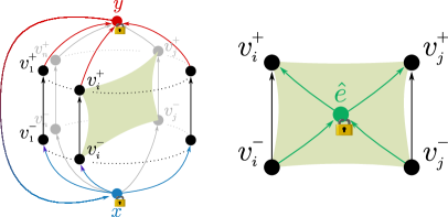
Figure 1. An illustration of the arcs in the reduced instance of Path-contraction Preserving Strong Connectivity. The second figure only contains the arcs of the edge-selection gadget corresponding to the edge $e=(v_{i},v_{j})\in E(G)$. Vertices with a padlock have additional $k+1$ pendant vertices with arcs in both directions.

We now consider the converse direction. Suppose that $(D,k)$ is a yes-instance of Path-contraction Preserving Strong Connectivity and let $S=\{a_{1},\dots,a_{k}\}$ be a solution for this instance. We require the following claim.

Claim 2.

For every edge $e=(u,v)\in E(G)$, $|S\cap\{(u^{-},u^{+}),(v^{-},v^{+})\}|\leqslant 1$. Furthermore, $S\subseteq\{(v^{-},v^{+})\mid v\in V(G)\}$.

Proof 3.3.

For the first statement, suppose to the contrary that $S$ contains both the arcs $(u^{-},u^{+})$ and $(v^{-},v^{+})$ for some $e=(u,v)\in E(G)$. Then, observe that in the graph $D\mathbin{/\mkern-6.0mu/}S$, the arcs in the set ${\mathcal{B}}_{e}$ are absent. Since ${\mathcal{B}}_{e}$ contains all arcs incident to $\hat{e}$ except the ones incident to $\hat{e}_{i}$ for $i\in[k+1]$, this disconnects the undirected graph underlying $D\mathbin{/\mkern-6.0mu/}S$, implying that $S$ is not a solution, a contradiction.

For the second statement, we argue that no arc incident to $x,y$ or $\{\hat{e}\mid e\in E(G)\}$ can be in $S$. Suppose to the contrary that for some $i\in[k+1]$, the arc $(x,x^{i})\in S$. Then, the arcs from $x$ to $\{v^{-}\mid v\in V(G)\}$ are all absent from $D^{\prime}$, implying that $D^{\prime}$ is not strongly connected, a contradiction. On the other hand, if for some $v\in V(G)$, we path-contract the arc $(x,v^{-})$, the arc from $x$ to $x^{i}$ is absent in $D\mathbin{/\mkern-6.0mu/}S$ for every $i\in[k+1]$. Since $|S|\leqslant k$, there is at least one $i\in[k+1]$ such that the arc $(x,x^{i})$ is not in $S$. Since the arc $(x,x^{i})$ is absent from $D\mathbin{/\mkern-6.0mu/}S$, it follows that it is not strongly-connected, a contradiction. Finally, if $S$ contains the arc $(y,x)$, the arc $(x^{i},x)$ is not in $D\mathbin{/\mkern-6.0mu/}S$ for any $i\in[k+1]$, implying that it is not strongly-connected for the same reason as that in the previous case. Hence, we conclude that no arc incident on $x$ is in $S$. The argument for $y$ is analogous and hence we do not address it explicitly.

Suppose that for some $e=(u,v)\in E(G)$ and $i\in[k+1]$, there is an arc in $\{(\hat{e},\hat{e}_{i}),(\hat{e}_{i},\hat{e})\}$ which is in $S$. Observe that in the former case, the arcs $(\hat{e},u^{+})$ and $(\hat{e},v^{+})$ are absent in $D\mathbin{/\mkern-6.0mu/}S$, implying that the new vertex is a sink, a contradiction. In the latter case, the new vertex is a source, a contradiction. Now, suppose that $S$ contains an arc in ${\mathcal{B}}_{e}$. Then, for some $i\in[k+1]$, the vertex $\hat{e}_{i}$ is left as a source or sink in $D\mathbin{/\mkern-6.0mu/}S$, a contradiction. This completes the proof of the claim.

The claim above implies that if $X$ is a solution for the reduced instance of Path-contraction Preserving Strong Connectivity, then the set $S$ of arcs corresponds independent set in $G$. In other words, $(G,k)$ is a yes-instance of Independent Set. This proves the correctness of the reduction and completes the proof of the theorem.

We can prove a similar result for the Vertex-deletion Preserving Strong Connectivity problem. The problem is formally defined as follows.

Problem 3.4 ($k$).

Vertex-deletion Preserving Strong Connectivity & A strongly connected digraph $D$ and an integer $k$.
Is there a vertex set $S$ of size (exactly) $k$ such that the graph $D-S$ is strongly connected?

We have to require “exactly $k$” rather than “at least $k$” since otherwise we could delete all but one vertices of $D$ and get a trivially strongly connected digraph.

See 1.6

Proof 3.5.

We will again use a reduction from Independent Set. Let $G$ be a graph, an input of Independent Set with parameter $k$. We first reduce Independent Set to Vertex-deletion Preserving Connectivity with Undeletable Vertices: Given a connected graph $H$ with some vertices marked and parameter $k$, is there $k$ unmarked vertices in $H$ whose deletion keeps $H$ connected? To construct $H$, start from $G$ with all vertices unmarked. Subdivide every edge of $G$ with a marked vertex. Add another marked vertex $x$ with edges to all unmarked vertices. It is easy to see that the reduction is correct since deleting two unmarked vertices in $H$ which are adjacent in $G$ leaves the corresponding subdivision vertex isolated.

Now we reduce Vertex-deletion Preserving Connectivity with Undeletable Vertices to Vertex-deletion Preserving Strong Connectivity. Replace every edge $uv$ of $H$ by arcs $uv$ and $vu$, unmark every marked vertex $w$ of $H$ and replace it by a directed cycle of length $k+2$ containing $w$ (all other vertices of the cycle are new). Denote the resulting digraph by $D$; note that it is strongly connected. To see the correctness, it suffices to observe that we cannot delete less than $k+1$ vertices of any directed cycle of length $k+2$ and keep $D$ strongly connected. This completes the proof of the theorem.

4. Edge deletion to biconnected graphs

In this section, we present our FPT algorithm for the Weighted Biconnectivity Deletion problem on undirected graphs. Recall that the problem is defined as follows:

Problem 4.1 ($k$).

Weighted Biconnectivity Deletion & A biconnected graph $G$, $k\in{\mathbb{N}}$, $w^{*}\in{\mathbb{R}}_{\geqslant 0}$ and a function $w:E(G)\to{\mathbb{R}}_{\geqslant 0}$.
Is there a set $S\subseteq E(G)$ of size at most $k$ such that $G-S$ is biconnected and $w(S)\geqslant w^{*}$?

We refer to a set $S\subseteq E(G)$ such that $G-S$ is biconnected as a biconnectivity deletion set of $G$. For an instance $(G,k,w^{*},w)$ of Weighted Biconnectivity Deletion and a biconnectivity deletion set $S$ of $G$, we say that $S$ is a solution if $|S|\leqslant k$ and $w(S)\geqslant w^{*}$. The main result of this section is the following.

See 1.2

We will first make a short digression in order to define the notion of critical edges and list certain structural properties that will be required in this and the following section.

4.1. Properties of critical edges

Definition 4.2.

We denote by $\kappa(G)$ the vertex-connectivity of a graph $G$. Let $G$ be a $\rho$-vertex connected graph. An edge $e\in E(G)$ is called $\rho$-critical if $\kappa(G-e)<\rho$. We denote by ${\sf Critical^{\rho}_{G}(e)}$ the subset of $E(G)$ comprising edges which are $\rho$-critical in $G-e$ but not in $G$. We denote by ${\sf Critical}^{\rho}_{G}(\emptyset)$ the set of edges which are already $\rho$-critical in $G$. In all notations, we ignore the explicit reference to $G$ and $\rho$ when these are clear from the context. We say that $e$ is $\rho$-critical for a pair of vertices $u,v$ in $G$ if $u$ and $v$ are non-adjacent and $e$ participates in every $u$-$v$ flow of value $\rho$ in $G$.

The following lemma gives a useful structural characterization of edges which become $\rho$-critical upon the deletion of a particular edge of the graph.

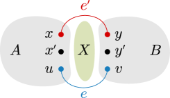
Figure 2. An illustration of the edges $e,e^{\prime}$ and the sets $A$ and $B$ in the proof of Lemma 4.3. Observe that there are no more edges with one endpoint each in $A$ and $B$.

Lemma 4.3.

Let $G$ be a $\rho$-vertex connected graph. Let $e=(x,y)$ and $e^{\prime}=(u,v)$ be distinct non-critical edges, they are not in ${\sf Critical}^{\rho}_{G}(\emptyset)$. Then the following are equivalent:

1. $e^{\prime}\in{\sf Critical}^{\rho}_{G}(e)$.

2. There is a pair of vertices $x^{\prime},y^{\prime}\in V(G)$ and a mixed $x^{\prime}$-$y^{\prime}$ cut $X$ of size $\rho$ in $G-e$, where $e^{\prime}\in X$.

3. $e^{\prime}$ participates in every $x$-$y$ flow of value $\rho$ in $G-e$.

Proof 4.4.

We prove that $(1)\Rightarrow(2)$, $(2)\Rightarrow(3)$ and $(3)\Rightarrow(1)$. Consider the first implication. Since $e^{\prime}\in{\sf Critical}^{\rho}_{G}(e)$, it must be the case that there are vertices $x^{\prime},y^{\prime}$ such that $e^{\prime}$ is $\rho$-critical for the pair $x^{\prime},y^{\prime}$. That is, $x^{\prime}$ is non-adjacent to $y^{\prime}$ and $e^{\prime}$ is $\rho$-critical for the pair $x^{\prime},y^{\prime}$ in $G^{\prime}=G-e$. That is, $e^{\prime}$ participates in every $x^{\prime}$-$y^{\prime}$ flow of value $\rho$ in $G-e$. As a result, the maximum value of any $x^{\prime}$-$y^{\prime}$ flow in $G-e-e^{\prime}$ is precisely $\rho-1$. By Menger’s theorem, this implies the presence of a set $S\subseteq V(G)$ of size $\rho-1$ which intersects all $x^{\prime}$-$y^{\prime}$ paths in $G-e-e^{\prime}$. Setting $X=S\cup\{e^{\prime}\}$ completes the argument for the first implication.

Consider the second implication. Let $A=R_{G-e}(x^{\prime},X)$ and let $B=V(G)\setminus(A\cup S)$ (see Figure 2), where $S=X\setminus\{e^{\prime}\}$. Observe that if $u,v\in A$ or $u,v\in B$, then $X\setminus\{e^{\prime}\}$ would be an $x^{\prime}$-$y^{\prime}$ separator of size $\rho-1$ in $G-e$, a contradiction to $G-e$ being $\rho$-vertex connected. Hence, it must be the case that either $u\in A$ and $v\in B$ or vice-versa. We assume without loss of generality that $u\in A$ and $v\in B$.

By a similar argument, since $e^{\prime}$ is not $\rho$-critical in $G$ but is $\rho$-critical in $G-e$, it must be the case that the edge $e$ also has one endpoint in $A$ and one endpoint in $B$. Again, we assume without loss of generality that $x\in A$ and $y\in B$. But now, observe that in the graph $G-e-S$, every $x$-$y$ path contains the edge $e^{\prime}$. Since $|S|=\rho-1$ and $G-e$ is $\rho$-connected, we conclude that $e^{\prime}$ participates in every $x$-$y$ flow of value $\rho$ in $G-e$. This completes the argument for the second implication.

For the final implication, observe that while $G-e$ is $\rho$-connected, the fact that $e^{\prime}$ participates in every $x$-$y$ flow of value $\rho$ in $G-e$ implies that $e^{\prime}$ is $\rho$-critical in $G-e$. Since $e^{\prime}$ is by definition, not $\rho$-critical in $G$, we conclude that $e^{\prime}\in{\sf Critical}^{\rho}_{G}(e)$. This completes the proof of the lemma.

4.2. The FPT algorithm for Weighted Biconnectivity Deletion

In this section, we will prove Theorem 1.2 by giving an algorithm for a more general version of the Weighted Biconnectivity Deletion problem where the input also includes a set $E^{\infty}\subseteq E(G)$ and the objective is to decide whether there is a solution disjoint from this set. Henceforth, instances of Weighted Biconnectivity Deletion will be of the form $(G,k,w^{*},w,E^{\infty})$ and any solution $S$ is required to be disjoint from $E^{\infty}$. We will refer to edges of $E(G)\setminus E^{\infty}$ as potential solution edges. We say that a potential solution edge is irrelevant if either the instance has no solution, or has a solution that does not contain $e$. For an instance $I=(G,k,w^{*},w,E^{\infty})$ and $r\in{\mathbb{N}}$, we denote by ${\sf Heavy}_{I}(r)$ the heaviest $r$ potential solution edges of $G$ with respect to the function $w$. While this set is not necessarily unique (if multiple edges have the same weight, i.e., the same image under the function $w$), we will define ${\sf Heavy}_{I}(r)$ as the first $r$ edges of a fixed arbitrarily chosen ordering of the edges of $G$ in non-increasing order of their weights. If $I$ is clear from the context, we simply write ${\sf Heavy}(r)$ when referring to ${\sf Heavy}_{I}(r)$.

Since we will only be dealing with biconnected graphs in this section, we will also drop the explicit reference to $\rho$ in the notations from Definition 4.2. For instance, when we say that an edge is critical (non-critical), we imply that it is 2-critical (not 2-critical respectively). Observe that no edge from the set ${\sf Critical}_{G}(\emptyset)$ can be part of a solution. As a result, we assume without loss of generality that for any instance $(G,k,w^{*},w,E^{\infty})$, the set ${\sf Critical}_{G}(\emptyset)$ is contained in $E^{\infty}$. Furthermore, since the edges in $E^{\infty}$ can never be part of a solution, we assume without loss of generality that for every edge $e\in E^{\infty}$, $w(e)=0$. The proof of Theorem 1.2 is based on the following lemma which states that either a) the number of potential solution edges in the instance is already bounded polynomially in $k$, or b) a ‘small’ set of the heaviest edges in the instance must intersect a solution, or c) there is an irrelevant edge which can be found in polynomial time. For ease of presentation, let use define the polynomial $\mu(x):=20x^{3}+46x^{2}+x$ for the rest of this section.

Lemma 4.5.

Let $I=(G,k,w^{*},w,E^{\infty})$ be an instance of Weighted Biconnectivity Deletion. If $|E(G)\setminus E^{\infty}|>\mu(k)$, then the set ${\sf Heavy}(\mu(k))$ contains either a solution edge or an irrelevant edge which can be computed in polynomial time.

Given Lemma 4.5, Theorem 1.2 is proved as follows. Let $I=(G,k,w,w^{*},E^{\infty})$ be an instance of Weighted Biconnectivity Deletion. If the number of potential solution edges in this instance is already bounded by $\mu(k)$, then we simply enumerate all $k$-sized subsets of this set (there are $2^{O(k\log k)}$ choices) and check in polynomial time whether one of these subsets is a solution. Otherwise, we invoke Lemma 4.5 and either correctly conclude that the set ${\sf Heavy}(\mu(k))$ contains a solution edge, or we compute an irrelevant edge $e$ in polynomial time. In the first case we branch on the set ${\sf Heavy}(\mu(k))$, reduce the budget $k$ by 1 and the target weight $w^{*}$ accordingly and recursively solve the resulting instance. In the second case, we add the edge $e$ to the set $E^{\infty}$ (thus decreasing the set of potential solution edges) and repeat.

Remark 4.6.

There is also an alternative strategy to the above, as follows. Let $S$ be the set of all edges of weight at least $w^{*}/k$. Clearly $S$ must be non-empty and any solution must intersect $S$. If $|S|\leqslant\mu(k)$, then we branch on $S$ as above. Otherwise, we will be able to either find a biconnectivity deletion set $S^{\prime}\subseteq S$ with $|S^{\prime}|=k$ or an irrelevant edge in $S$ as in Lemma 4.5. In the former case, $S^{\prime}$ is already a solution; in the latter case, we proceed according to the strategy above. Thus, this alternative strategy yields a slightly simpler proof, contains one less branching step and will be used in the kernelization algorithm in Subsection 4.3. On the other hand, the strategy above does not explicitly depend on $w^{*}$, and therefore always gives a maximum-weight solution. In either case, the main technical challenges in the FPT algorithm are exactly the same.

The rest of this section is devoted to proving Lemma 4.5. In order to do so, we will present a greedy algorithm that runs in polynomial time and, assuming $|E(G)\setminus E^{\infty}|>\mu(k)$, will either produce a biconnectivity deletion set of size $k$ contained strictly within ${\sf Heavy}(\mu(k))$, or it will identify an irrelevant edge. In the former case, we will argue that this implies that there is always a solution intersecting ${\sf Heavy}(\mu(k))$. More precisely, the algorithm will delete one potential solution edge from ${\sf Heavy}(\mu(k))$ at a time (while preserving biconnectivity), and will trace in each step the number of edges of ${\sf Heavy}(\mu(k))$ that become critical due to the removal of such an edge $e$, i.e., the size of the set ${\sf Critical}_{G^{\prime}}(e)\cap{\sf Heavy}(\mu(k))$ where $G^{\prime}$ is the subgraph of $G$ remaining after deleting the edges before $e$. We will then show that if $|{\sf Critical}_{G^{\prime}}(e)\cap{\sf Heavy}(\mu(k))|\geqslant\frac{\mu(k)-k}{k}$, then $G$ contains a special configuration from which we can either recover the required biconnectivity deletion set or identify an irrelevant edge.

4.2.1. Preliminary results

From now on, we assume that the given instance has more than $\mu(k)$ potential solution edges and begin by proving the following lemma which shows that if we find some biconnectivity deletion set of size $k$ within ${\sf Heavy}(\mu(k))$, then there is a solution intersecting ${\sf Heavy}(\mu(k))$.

Lemma 4.7.

Let $I=(G,k,w^{*},w,E^{\infty})$ be an instance of Weighted Biconnectivity Deletion and let $S\subseteq{\sf Heavy}(\mu(k))$ be a biconnectivity deletion set of size $k$. If $I$ is a yes-instance, then there is a solution for $I$ intersecting the set ${\sf Heavy}(\mu(k))$.

Proof 4.8.

Suppose that this is not the case and let $S^{\prime}$ be a biconnectivity deletion set of size at most $k$ such that $w(S^{\prime})\geqslant w^{*}$. Note that $S^{\prime}$ is disjoint from ${\sf Heavy}(\mu(k))$ and $S$ is contained in ${\sf Heavy}(\mu(k))$. Since $|S^{\prime}|\leqslant|S|$, we infer that $w(S)\geqslant w(S^{\prime})$, a contradiction to our assumption that there is no solution intersecting ${\sf Heavy}(\mu(k))$. This completes the proof of the lemma.

Let $\hat{S}=\{f_{1},\dots,f_{r}\}\subseteq{\sf Heavy}(\mu(k))$ be a set greedily constructed as follows. The edge $f_{1}$ is the heaviest potential solution edge. That is, $w(f_{1})\geqslant w(e)$ for every $e\in E(G)\setminus E^{\infty}$. For each $2\leqslant i\leqslant r$, $f_{i}$ is the heaviest edge of ${\sf Heavy}(\mu(k))$ which is not critical in $G-\{f_{1},\dots,f_{i-1}\}$. We terminate this procedure after $k$ steps if we manage to find edges $\{f_{1},\dots,f_{k}\}$ or earlier if for some $r<k$, every edge of ${\sf Heavy}(\mu(k))$ is critical in $G-\{f_{1},\dots,f_{r}\}$.

Observe that by definition, $\hat{S}$ is a biconnectivity deletion set. Therefore, if $r=k$, then Lemma 4.7 implies that if there is a solution for the given instance, then there is one intersecting ${\sf Heavy}(\mu(k))$ (as required in Lemma 4.5). On the other hand, suppose that $r<k$. For each $i\in[r]$, we denote by $\hat{S}_{i}$, the set $\{f_{1},\dots,f_{i}\}$ and by $\hat{S}_{0}$, the empty set. Recall that we have already assumed that the number of potential solution edges is greater than $\mu(k)=20k^{3}+46k^{2}+k$. As a result, we have the following observation.

Observation 4.9.

There is an $i\in[r]$ such that $G-\hat{S}_{i}$ is biconnected and $|{\sf Critical}_{G-\hat{S}_{i-1}}(f_{i})\cap{\sf Heavy}(\mu(k))|\geqslant\frac{\mu(k)-k}{k}=20k^{2}+46k$.

Let $i\in[r]$ be the index referred to in this observation. In the rest of the section, we let $\hat{F}=\hat{S}_{i-1}$, $e=f_{i}=(x,y)$ and $G^{\prime}=G-\hat{F}$. The following observation is a straightforward consequence of Lemma 4.3 in our setting.

Observation 4.10.

Let $G^{\prime}$ and $e$ be as above. Then, $\kappa_{G^{\prime}-e}(x,y)=2$ and for any $x$-$y$ flow ${\mathcal{H}}=\{H_{1},H_{2}\}$ of value 2 in $G^{\prime}-e$, the following holds.

1. Every edge of ${\sf Critical}_{G^{\prime}}(e)$ is critical for the pair $x,y$ in $G^{\prime}-e$ and hence lies on $H_{1}$ or $H_{2}$.

2. For every edge $e_{1}\in{\sf Critical}_{G^{\prime}}(e)$, say on $H_{1}$, there is at least one vertex $v$ on $H_{2}$ such that $\{e_{1},v\}$ is a mixed $x$-$y$ cut in $G^{\prime}-e$.

We refer to the vertex $v$ above as a partner vertex of $e_{1}$, and refer to the set of all partner vertices of $e_{1}$ as the partner set of $e_{1}$ and denote this set by ${\sf Partner}^{e}_{G^{\prime}-e}(e_{1})$. We do not explicitly refer to $H_{1}$ or $H_{2}$ in this notation because these will always be clear from the context. We will also drop the explicit reference to $G^{\prime}$ and $e$ when these are clear from the context.

From Observation 4.9 and Obsevation 4.10, we now conclude the following:

Observation 4.11.

Let $G^{\prime}$ and $e$ be as above. There is an $x$-$y$ flow ${\mathcal{P}}=\{P_{1},P_{2}\}$ of value 2 in $G^{\prime}-e$ such that $|E(P_{1})\cap{\sf Critical}_{G^{\prime}}(e)\cap{\sf Heavy}(\mu(k))|\geqslant 10k^{2}+23k$.

Henceforth, we work with this fixed $x$-$y$ flow ${\mathcal{P}}=\{P_{1},P_{2}\}$ in $G^{\prime}-e$.

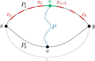
Figure 3. An illustration of ${\sf Segment}[i,i+1]$ (the subpath of $P_{1}$ between $e_{i}$ and $e_{i+1}$) and $P$ which is a nice path for this segment.

Definition 4.12.

Let $G^{\prime}$,$e=(x,y),P_{1}$ and $P_{2}$ be as above. Let $e_{1},\ldots,e_{t}$ be some subset of $10k^{2}+23k$ edges in ${\sf Critical}_{G^{\prime}}(e)\cap{\sf Heavy}(\mu(k))\cap E(P_{1})$ in the order in which they appear when traversing $P_{1}$ from $x$ to $y$ (see Figure 3), where $e_{i}=(u_{i},v_{i})$ and we may have $v_{i}=u_{i+1}$.

• For $i\in[t-1]$, we refer to the subpath of $P_{1}$ from $v_{i}$ to $u_{i+1}$ inclusively as ${\sf Segment}[i,i+1]$ of $P_{1}$ with the explicit reference to $P_{1}$ dropped when clear from the context.

• A path $P$ with endpoints $u,v\in V(P_{1})\cup V(P_{2})$ but internally vertex-disjoint from $P_{1}$ and $P_{2}$ is said to be a nice path for ${\sf Segment}[i,i+1]$ if $u$ is contained in ${\sf Segment}[i,i+1]$ and $v\in V_{\sf int}(P_{2})$.

When $e$, $P_{1}$, $P_{2}$ are as in the definition above, we write $w\leqslant w^{\prime}$ for vertices $w,w^{\prime}\in V(P_{2})$ if either $w=w^{\prime}$ or $w$ is encountered before $w^{\prime}$ when traversing $P_{2}$ from $x$ to $y$, and similarly for vertices on $P_{1}$. Furthermore, for a set $Q\subseteq V(P_{2})$ and vertex $w\in V(P_{2})$, we say that $w<Q$ ($w>Q$) if $w<q$ ($w>q$ respectively) for every $q\in Q$. We need the following crucial structural lemma regarding the structure of any path with endpoints in $P_{1}$ and $P_{2}$ but which is otherwise disjoint from these two paths.

Lemma 4.13.

Let $G^{\prime},e=(x,y),P_{1},P_{2}$, $e_{1},\dots,e_{t}$ be as above. Let $P$ be a path in $G^{\prime}$ with endpoints $u,v\in V(P_{1})\cup V(P_{2})$ but internally vertex-disjoint from $P_{1}$ and $P_{2}$. Then the following statements hold.

1. If $u,v\in V(P_{1})$, then either $u,v\leqslant u_{1}$, or $u,v\geqslant v_{t}$, or there is a $j\in[t-1]$ such that $u,v$ lie on ${\sf Segment}[j,j+1]$.

2. If $u,v\in V(P_{2})$, then the subpath of $P_{2}$ from $u$ to $v$ is internally vertex-disjoint from the set $\bigcup^{t}_{i=1}{\sf Partner}^{e}_{G^{\prime}}(e_{i})$.

3. If $u\in V(P_{1})$ and $v\in V(P_{2})$, where $u$ lies in ${\sf Segment}[i,i+1]$, then for every $j\leqslant i$ and every vertex $w\in{\sf Partner}(e_{j})$ we have $w\leqslant v$, and for every $j\geqslant i+1$ and every vertex $w\in{\sf Partner}(e_{j})$ we have $w\geqslant v$.

4. For every $i\in[t-1]$, there is at least one nice path for ${\sf Segment}[i,i+1]$, and for any $i\neq j\in[t-1]$, and paths $P$ and $P^{\prime}$ which are nice paths for ${\sf Segment}[i,i+1]$ and ${\sf Segment}[j,j+1]$ respectively, $P$ and $P^{\prime}$ are internally vertex-disjoint.

Proof 4.14.

For the first statement, suppose that there is an index $i\in[t]$ such that $u\leqslant u_{i}$ but $v\geqslant v_{i}$. Since $e_{i}$ is critical in $G^{\prime}-e$, Observation 4.10 implies that there is a mixed $x$-$y$ cut $X=\{e_{i},q\}$ where the vertex $q$ lies on $P_{2}$. However, the graph induced on $V(P_{1})\cup V(P)$ contains an $x$-$y$ path disjoint from $X$, a contradiction. This completes the argument for the first statement.

The argument for the second statement is similar. Suppose to the contrary that there is an $i\in[t]$ and a vertex $w\in{\sf Partner}(e_{i})$ such that the subpath of $P_{2}$ from $u$ to $v$ contains the vertex $w$. Recall that due to Observation 4.10, the set $X=\{e_{i},w\}$ is a mixed $x$-$y$ cut in $G^{\prime}-e$. But then $u\in R_{G^{\prime}-e}(x,X)$, $v\in R_{G^{\prime}-e}(y,X)$, and the path $P$ is disjoint from $X$, which contradicts $X$ being an $x$-$y$ cut.

For the third statement, suppose that there is a $j\leqslant i$ and $w\in{\sf Partner}(e_{j})$ such that $w>v$. Let $X=\{e_{j},w\}$. Due to Observation 4.10, we know that $X$ is a mixed $x$-$y$ cut in $G^{\prime}-e$. Let $A=R_{G^{\prime}-e}(x,X)$ and $B=R_{G^{\prime}-e}(y,X)$. Since $u\in{\sf Segment}[i,i+1]$ and $j\leqslant i$, it follows that $u\in B$. Similarly, since $w>v$, it must be the case that $v\in A$. As above, we find that $P$ is a path disjoint from $X$ connecting $A$ and $B$, which contradicts that $X$ is an $x$-$y$ cut. The argument for the case when there is a $j\geqslant i$ and $w\in{\sf Partner}(e_{j})$ such that $w<v$ is analogous.

For the first part of the final statement, assume for a contradiction that for some $i\in[t-1]$, the path ${\sf Segment}[i,i+1]$ does not have a nice path. Recall that $e_{i}$ is not critical in $G^{\prime}$ but is critical in $G^{\prime}-e$. Therefore, there is a $u_{i}$-$v_{i}$ flow of value 2 in the graph $G^{\prime}-e_{i}$; let ${\mathcal{H}}=\{H_{1},H_{2}\}$ be such a flow. If $H_{1}$ or $H_{2}$ intersects the internal vertices of $P_{2}$, then this implies the presence of a nice path for ${\sf Segment}[i,i+1]$. Hence, we assume that this does not happen. We also conclude that $e$ must occur in $H_{1}$ or $H_{2}$. Indeed, observe that $e$ is critical in $G^{\prime}-e_{i}$, since $G^{\prime}-e_{i}$ is biconnected but $G^{\prime}-e-e_{i}$ is not. Hence $e\in{\sf Critical}_{G^{\prime}}(e_{i})$, and by Lemma 4.3, $e$ must participate in ${\mathcal{H}}$. We may assume without loss of generality that $H_{1}$ contains the edge $e$. But now $H_{2}$ is a path from $u_{i}$ to $v_{i}$ in $G^{\prime}$, disjoint from both $e$, $e^{\prime}$, and $V_{\sf{int}}(P_{2})$. Clearly, $H_{2}$ contains a subpath $P$ in contradiction to the first statement of the present lemma. We conclude that for every $i\in[t-1]$, ${\sf Segment}[i,i+1]$ has a nice path.

For the second part of the last statement, let $P$ and $P^{\prime}$ be paths as described which are not internally vertex-disjoint. Then $P\cup P^{\prime}$ contains a walk, and therefore also a path, with endpoints in $V(P_{1})$, internally vertex-disjoint from $V(P_{1})\cup V(P_{2})$, and with endpoints in distinct segments on $P_{1}$, in contradiction with the first statement of this lemma. This completes the argument for the last statement and hence the proof of the lemma.

Let us now consider how partner sets can intersect.

Observation 4.15.

Let $G^{\prime},e=(x,y),P_{1},P_{2}$, $e_{1},\dots,e_{t}$ be as above. Let $e_{i},e_{j}$ be a pair of edges, $1\leqslant i<j\leqslant t$, let $w_{1},\ldots,w_{r}$ be the partner vertices of $e_{i}$ in the order they appear on $P_{2}$, and let $w_{1}^{\prime},\ldots,w_{s}^{\prime}$ be the partner vertices of $e_{j}$ in the order they appear on $P_{2}$. Then $w_{i}\leqslant w_{j}^{\prime}$ for every $i\in[r]$, $j\in[s]$. In particular, the set ${\sf Partner}(e_{i})\cap{\sf Partner}(e_{j})$ can consist of at most one vertex $w$, which must then be the last vertex of ${\sf Partner}(e_{i})$ and the first vertex of $partner(e_{j})$ which is encountered when traversing $P_{2}$ from $x$ to $y$.

Proof 4.16.

Let $w_{i}\in{\sf Partner}(e_{i})$ and $w_{j}^{\prime}\in{\sf Partner}(e_{j}).$ By Lemma 4.13 (4), ${\sf Segment}[i,i+1]$ has a nice path $P$ with endpoints $u\in V(P_{1})$ and $v\in V(P_{2})$. By Lemma 4.13 (3), we have $w_{i}\leq v\leq w_{j}^{\prime}$. Thus, $w_{i}\leq w_{j}^{\prime}$ and the claim follows.

Thus, there is a well-defined first and last element for each partner set and these two elements (they may coincide) define a subpath of $P_{2}.$ Furthermore, the two subpaths corresponding to the partner sets of any two critical edges on $P_{1}$ do not have a ‘strict’ overlap and can only intersect in one vertex – their respective endpoints.

Having identified some of the structure in the graph, we now proceed to examine two cases. Recall that by Observation 4.11, the path $P_{1}$ contains at least $10k^{2}+23k$ edges of ${\sf Critical}_{G^{\prime}}(e)\cap{\sf Heavy}(\mu(k))$. We will consider one of two cases: either there is a sufficiently large number of distinct partner sets, or there is a sufficiently large number of critical edges with identical partner sets. We show how to handle each case in turn.

4.2.2. Many distinct partner sets

We first handle the first case, by formally arguing that if there are sufficiently many distinct partner sets, then ${\sf Heavy}(\mu(k))$ contains a solution edge. We begin with an observation about connectivity.

Lemma 4.17.

Let $G^{\prime},e=(x,y),P_{1},P_{2}$, $e_{1},\dots,e_{t}$ be as above. For each $i\in[t]$, there is a pair of internally vertex-disjoint $u_{i}$-$v_{i}$ paths $P_{a}$, $P_{b}$ in $G^{\prime}-e_{i}$ as follows.

1. $P_{a}$ contains the edge $e$. Additionally, if $i>1$, then $P_{a}$ either contains $e_{i-1}$ or intersects ${\sf Partner}(e_{i-1})$, and if $i<t$, then $P_{a}$ either contains $e_{i+1}$ or intersects ${\sf Partner}(e_{i+1})$.

2. $P_{b}$ has an endpoint each in ${\sf Segment}[i-1,i]$ and ${\sf Segment}[i,i+1]$, but does not intersect $P_{1}$ anywhere else except in these segments,

3. $P_{b}$ contains the set ${\sf Partner}(e_{i})$ and is disjoint from the set ${\sf Partner}(e_{j})\setminus{\sf Partner}(e_{i})$ for any $j\in[t]$, $j\neq i$, except possibly the vertices of $\bigcup_{j}{\sf Partner}(e_{j})$ immediately preceding and succeeding ${\sf Partner}(e_{i})$ on $P_{2}$.

Proof 4.18.

Let $(P_{a},P_{b})$ be a pair of internally vertex-disjoint $u_{i}$-$v_{i}$ paths in $G^{\prime}-e_{i}$. This exists since $e_{i}$ is not critical in $G^{\prime}$. Let $w\in{\sf Partner}(e_{i})$. Since $\{w,e_{i}\}$ is a mixed $x$-$y$ cut in $G^{\prime}-e$, it follows that $\{w,e\}$ is a mixed $u_{i}$-$v_{i}$ cut in $G^{\prime}-e_{i}$. Hence one path, say $P_{a}$, must pass through $e$, and the other must pass through $w$. Since $w$ was arbitrarily chosen, we find that $P_{b}$ contains every vertex of ${\sf Partner}(e_{i})$. Next, assume $i>1$ and let $w^{\prime}$ be the largest vertex in ${\sf Partner}(e_{i-1})$ in the order $<$. Then $\{w^{\prime},e_{i-1}\}$ is a mixed $x$-$y$ cut in $G^{\prime}-e$, thus $P_{a}$ must pass through either $e_{i-1}$ or $w^{\prime}$ on the way from $u_{i}$ to $x$. The dual argument holds for $e_{i+1}$ if $i<t$. This covers the first property. For the second and third properties, consider again the mixed cut $\{e_{i-1},w^{\prime}\}$. Since $P_{b}$ contains $u_{i}$ and $v_{i}$, both of which are on the same side in the above cut, $P_{b}$ passes through the cut an even number of times; since $P_{a}$ intersects the cut, $P_{b}$ cannot pass through the cut and so cannot intersect $P_{1}$ in any segment before ${\sf Segment}[i-1,i]$, nor $P_{2}$ in any vertex before $w^{\prime}$. (Note that $P_{b}$ may intersect $w^{\prime}$, but it cannot intersect any vertex on the other side of the cut.) An analogous argument holds for $e_{i+1}$ if $i<t$.

We now state and prove the lemma which handles the first case, there are a sufficiently large number of distinct partner sets.

Lemma 4.19.

Let $G^{\prime},e=(x,y),P_{1},P_{2}$, $e_{1},\dots,e_{t}$ be as above. Assume that there are more than $3k$ distinct partner sets for the edges $e_{1},\dots,e_{t}$. Then the instance $(G,k,w^{*},w,E^{\infty})$ has a solution intersecting ${\sf Heavy}(\mu(k))$.

Proof 4.20.

Let $Z=\{e_{1},\dots,e_{t}\}$ and let $e_{i_{1}}$, …, $e_{i_{3k+1}}$, be a subset of $Z$ such that for every $1\leqslant p<q\leqslant 3k+1$, (a) $i_{q}>i_{p}$ and (b) ${\sf Partner}(e_{i_{p}})\neq{\sf Partner}(e_{i_{q}})$. Let $S=\{e_{i_{1}},e_{i_{4}},\ldots,e_{i_{3k-2}}\}$. Clearly $|S|=k$; we claim that $S$ is a biconnectivity deletion set for $G^{\prime}$.

To see this, let $e_{i_{j}}=(u_{i_{j}},v_{i_{j}})$ be an arbitrary edge of $S$, and let $P_{a}$, $P_{b}$ be $(u_{i_{j}},v_{i_{j}})$-paths given by Lemma 4.17. Then the path $P_{b}$ remains in $G^{\prime}-S$; we will reconfigure $P_{a}$ to be disjoint from $S$. We will create a path $P=P_{x}+(x,y)+P_{y}$, by separately providing a path $P_{x}$ from $u_{i_{j}}$ to $x$ and a path $P_{y}$ from $v_{i_{j}}$ to $y$ which are disjoint from $P_{b}$ and neither of which contains the edge $e=(x,y)$. If $j=1$, then $e_{i_{j}}$ is the first edge of $S$ along $P_{1}$ and we may simply use $P_{a}$ from $u_{i_{j}}$ to $x$ as $P_{x}$, so assume $j>1$. If $P_{a}$ intersects ${\sf Partner}(e_{i_{j}-1})$, then we may produce $P_{x}$ by continuing along $P_{2}$ to $x$. Otherwise $P_{a}$ uses the edge $e_{i_{j}-1}$. In this case, produce $P_{x}$ by continuing along $P_{1}$ to ${\sf Segment}[i_{j-3},i_{j-3}+1]$, follow a nice path from this segment to $P_{2}$, and continue along $P_{2}$ to $x$.

We argue that the resulting path $P_{x}$ is disjoint from $P_{b}$. If $j=1$, then the claim is trivial. If $P_{a}$ intersects ${\sf Partner}(e_{i_{j}-1})$, then recall that $P_{a}$ and $P_{b}$ are internally disjoint, $P_{b}$ intersects ${\sf Partner}(e_{i_{j}})$, and ${\sf Partner}(e_{i_{j}-1})\leqslant{\sf Partner}(e_{i_{j}})$. Thus $P_{x}$ lies entirely before $P_{b}$ on $P_{2}$. Otherwise, $P_{x}$ uses a nice path $P$ from ${\sf Segment}[i_{j-3},i_{j-3}+1]$. The initial part of $P_{x}$ follows $P_{a}$, which is disjoint from $P_{b}$ by Lemma 4.17; the part between $u_{i_{j}-1}$ and $P$ is disjoint from $P_{b}$ by Lemma 4.17(2); and $V_{\sf int}(P)$ is disjoint from $P_{b}$ by Lemma 4.13(4). Let $q$ be the endpoint of $P$ on $P_{2}$, and let $w$ be the first vertex of ${\sf Partner}(e_{i_{j-2}})$ on $P_{2}$. Then $q\leqslant w$ by Lemma 4.13(3), and we claim $w<V(P_{b})\cap V(P_{2})$. Note that $w\notin{\sf Partner}(e_{i_{j}})$ since the three sets ${\sf Partner}(e_{i_{j-2}})$, ${\sf Partner}(e_{i_{j-1}})$, ${\sf Partner}(e_{i_{j}})$ are distinct and by Observation 4.15, let $w^{\prime}$ be the first vertex of ${\sf Partner}(e_{i_{j}})$ on $P_{2}$. Assume for a contradiction that $P_{b}$ intersects $w$. Then $P_{b}$ provides a path from $w$ to $e_{i_{j}}$ that avoids $e_{i_{j-1}}$ and $w^{\prime}$; hence $w^{\prime}\notin{\sf Partner}(e_{i_{j-1}})$ and ${\sf Partner}(e_{i_{j-1}})\cap{\sf Partner}(e_{i_{j}})=\emptyset$. But since ${\sf Partner}(e_{i_{j-2}})\neq{\sf Partner}(e_{i_{j-1}})$, there must be at least one further vertex $w^{\prime\prime}\in{\sf Partner}(e_{i_{j-1}})$ such that $w<w^{\prime\prime}<w^{\prime}$; this contradicts that $P_{b}$ intersects $w$ by Lemma 4.13. Thus $P_{x}$ and $P_{b}$ are internally vertex-disjoint. The argument for $P_{y}$ is analogous to that for $P_{x}$. Now $P_{a}=P_{x}+(x,y)+P_{y}$ and $P_{b}$ form a pair of internally vertex-disjoint $u_{i_{j}}$-$v_{i_{j}}$-paths, and since $e_{i_{j}}\in S$ was chosen arbitrarily, we conclude that $G^{\prime}-S$ is biconnected. Since $G$ is a supergraph of $G^{\prime}$, $G-S$ is also biconnected.

Finally, it follows from Lemma 4.7 that since $S\subseteq{\sf Heavy}(\mu(k))$ is a biconnectivity deletion set of size $k$ for $G$, there is a solution for the given instance intersecting ${\sf Heavy}(\mu(k))$. This completes the proof of the lemma.

4.2.3. Identical partner sets

Due to Lemma 4.19, we assume that there are at most $3k$ distinct partner sets for the edges of ${\sf Critical}_{G^{\prime}}(e)\cap{\sf Heavy}(\mu(k))$ which lie on $P_{1}$. Let $e_{1},\ldots,e_{t}$ be the set of all edges of ${\sf Critical}_{G^{\prime}}(e)\cap{\sf Heavy}(\mu(k))\cap E(P_{1})$, in the order they appear on $P_{1}$ from $x$ to $y$. We define a set of exceptional edges; initially we set $\hat{I}=\{1\leqslant i<t\mid{\sf Partner}(e_{i})\neq{\sf Partner}(e_{i+1})\}$ (later we will define further exceptional edges). Then $|\hat{I}|\leqslant 3k$ by Observation 4.15; we study the structure of contiguous stretches of edges $e_{i}$, …, $e_{j}$ with indices disjoint from $\hat{I}$. Note that all edges in such a stretch have identical partner sets. We make an observation about the structure.

Lemma 4.21.

Let $Z=\{e_{i},\ldots,e_{j}\}$ be a set of edges of ${\sf Critical}_{G^{\prime}}(e)\cap{\sf Heavy}(\mu(k))\cap E(P_{1})$ such that for every $i\leqslant i^{\prime}<j^{\prime}\leqslant j$, $e_{i^{\prime}}$ occurs before $e_{j^{\prime}}$ when traversing $P_{1}$ from $x$ to $y$ and ${\sf Partner}_{G^{\prime}-e}(e_{i})={\sf Partner}_{G^{\prime}-e}(e_{j})$. Then the following hold:

1. $|{\sf Partner}_{G^{\prime}-e}(e_{i^{\prime}})|=1$ and ${\sf Partner}_{G^{\prime}-e}(e_{i^{\prime}})$ = ${\sf Partner}_{G^{\prime}-e}(e_{i})$ for every $i\leqslant i^{\prime}\leqslant j$, say ${\sf Partner}_{G^{\prime}-e}(e_{i^{\prime}})=\{w\}$;

2. For every $i\leqslant i^{\prime}<j$ and nice path $P$ for ${\sf Segment}[i^{\prime},i^{\prime}+1]$, $V(P)\cap V(P_{2})=\{w\}$.

Proof 4.22.

The first statement follows from Observation 4.15: since ${\sf Partner}_{G^{\prime}-e}(e_{i})$ and ${\sf Partner}_{G^{\prime}-e}(e_{j})$ can intersect in at most one vertex, we have $|{\sf Partner}_{G^{\prime}-e}(e_{i})|=1$, and since partner sets appear in an “ordered” way on $P_{2}$, we have ${\sf Partner}_{G^{\prime}-e}(e_{i^{\prime}})={\sf Partner}_{G^{\prime}-e}(e_{i})$ for every $i<i^{\prime}\leqslant j$. The second statement follows from the third statement of Lemma 4.13.

In light of Lemma 4.21, for any edge $e_{i}$ with $i\notin\hat{I}$, we let $w(i)$ denote the single partner vertex of $e_{i}$, i.e., ${\sf Partner}_{G^{\prime}-e}(e_{i})=\{w(i)\}$.

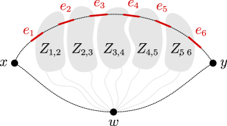
Figure 4. An illustration of the sets $\{{\sf Component}[i,i+1]\mid i\in[t-1]\}$ for $t=6$, where the set $Z_{i,i+1}$ represents ${\sf Component}[i,i+1]$. Note that it is possible that ${\sf Component}[i,i+1]$ contains a single vertex, in which case this vertex must be the same as both $v_{i}$ and $u_{i+1}$.

Definition 4.23.

For each $1\leqslant i<t$ with $i\notin\hat{I}$, we define ${\sf Component}[i,i+1]$ as the set of vertices reachable from $V({\sf Segment}[i,i+1])$ in the graph $G^{\prime}-\{e_{i},e_{i+1},w(i)\}$ (see Figure 4). We let $\Gamma[i,i+1]$ denote the edge set $E({\sf Component}[i,i+1])\cup E(w(i),{\sf Component}[i,i+1])$.

Observation 4.24.

Let $Z=[t]\setminus\hat{I}$ be the indices of non-exceptional edges $e_{i}$. The following hold.

• For every $i\in Z$, ${\sf Segment}[i,i+1]$ is contained in ${\sf Component}[i,i+1]$.

• For every $i\in Z$, $N_{G^{\prime}}({\sf Component}[i,i+1])=\{u_{i},v_{i+1},w(i)\}$.

• For every pair $i,j\in Z$, $i\neq j$, the sets ${\sf Component}[i,i+1]$ and ${\sf Component}[j,j+1]$ are vertex-disjoint and they are disjoint from $V(P_{2})$.

• For every pair $i,j\in Z$, $i\neq j$, $\Gamma[i,i+1]$ and $\Gamma[j,j+1]$ are disjoint.

Proof 4.25.

The first and second statements follow from the definition of ${\sf Component}[i,i+1]$. For the third statement, the second statement of Lemma 4.21 implies that ${\sf Component}[i,i+1]$ is disjoint from $V(P_{2})$ and the first statement of Lemma 4.13 implies that for every $i\neq j$, the sets ${\sf Component}[i,i+1]$ and ${\sf Component}[j,j+1]$ are vertex-disjoint. The final statement is a direct consequence of the third statement. This completes the proof.

We need to consider one further complication. Recall that $\hat{F}$, as defined after Observation 4.9, denote the edges removed from the original graph $G$ to create $G^{\prime}$.

Definition 4.26.

For each $1\leqslant i\leqslant t-1$, $i\notin\hat{I}$, we say that ${\sf Component}[i,i+1]$ is affected if the set $\hat{F}$ has an endpoint in ${\sf Component}[i,i+1]$ and unaffected otherwise.

Since $|\hat{F}|<k$, it follows that fewer than $2k$ of these disjoint vertex-sets can be affected. We will treat these as a secondary set of exceptional indices; let $\hat{J}=\{i\in[t]\setminus\hat{I}\mid{\sf Component}[i,i+]\text{ is affected}\}$. We make a final observation.

Observation 4.27.

Let $e_{1},\ldots,e_{t}$ be as above, with $t\geqslant 10k^{2}+23k$. Then there is a contiguous sequence $a,\ldots,b\in[t]$ of indices such that $b\geqslant a+2k+3$ and for every integral $i\in[a,b]$, ${\sf Partner}(e_{i})={\sf Partner}(e_{a})$ and ${\sf Component}[i,i+1]$ is unaffected.

Proof 4.28.

We have $|\hat{I}|\leqslant 3k$ and $|\hat{J}|\leqslant 2k-2$, hence $[t]\setminus(\hat{I}\cup\hat{J})$ decomposes into at most $5k-1$ parts. With $t\geqslant(2k+4)(5k-1)+5k-2=10k^{2}+23k-6$, one of these parts will contain at least $2k+4$ indices, hence its bounding indices $a,b$ will satisfy $b\geqslant a+2k+3$.

We refer to such a sequence $e_{a},\ldots,e_{b}$ of edges as an clean stretch of $P_{1}$. The remaining task towards the FPT algorithm is to show that a sufficiently long clean stretch contains an irrelevant edge.

4.2.4. Reducing clean stretches

We will now restrict our attention to a single clean stretch $[a,b]$, and prove that it contains an irrelevant edge. To simplify the notation, let $w=w(a)$. We have the following lemma, where $\delta_{H}(Q)$ denotes the edges of $H$ with one endpoint in $Q$.

Lemma 4.29.

Let $G^{\prime}=G-\hat{F}$ be as above and let $Z=\{e_{a},\ldots,e_{b}\}$ be a clean stretch. Then for every $a\leqslant i<b$, (a) ${\sf Component}[i,i+1]$ is unaffected, (b) $N_{G^{\prime}}({\sf Component}[i,i+1])$ = $N_{G}({\sf Component}[i,i+1])=\{u_{i},v_{i+1},w\}$ and (c) $\delta_{G^{\prime}-w}({\sf Component}[i,i+1])=\delta_{G-w}({\sf Component}[i,i+1])=\{e_{i},e_{i+1}\}$.

Proof 4.30.

Statement (a) holds by definition. For statements (b) and (c), the neighbourhoods and incident edges are the same in $G$ as in $G^{\prime}$ since the components are unaffected, and it follows from the definition of ${\sf Component}[i,i+1]$ that $N_{G^{\prime}}({\sf Component}[i,i+1])=\{u_{i},v_{i+1},w\}$ and $\delta_{G^{\prime}-w}({\sf Component}[i,i+1])=\{e_{i},e_{i+1}\}$.

Lemma 4.31.

Let $G^{\prime},Z=\{e_{a},\dots,e_{b}\}$ be as above. For any $i\in[a+1,b-1]$, the following hold:

1. There is a $v_{i}$-$\{w,u_{i+1}\}$ flow of value 2 in the graph $G[{\sf Component}[i,i+1]\cup\{w\}]$.

2. There is a $u_{i}$-$\{w,v_{i-1}\}$ flow of value 2 in the graph $G[{\sf Component}[i-1,i]\cup\{w\}]$.

Proof 4.32.

We show the first statement; the proof of the second is analogous. If $v_{i}=u_{i+1}$, then the statement follows by considering the single-vertex path $v_{i}$ in combination with the nice path for ${\sf Segment}[i,i+1]$, hence assume that $v_{i}\neq u_{i+1}$. Since $e_{i}$ is not critical in $G^{\prime}$ it follows that there is a $u_{i}$-$v_{i}$ flow of value 2 in $G^{\prime}-e_{i}$. However, observe that due to Lemma 4.29, $\{w,u_{i+1}\}$ is a $u_{i}$-$v_{i}$ separator in $G^{\prime}-e_{i}$. Hence of the two paths of the flow, one contains $w$ and the other contains $u_{i+1}$. Truncating these paths at $w$ and at $u_{i+1}$ produces a flow in $G^{\prime}$. By Lemma 4.29, this truncated flow must remain in $G^{\prime}[{\sf Component}[i,i+1]\cup\{w\}]$, and since $G$ is a supergraph of $G^{\prime}$ it also exists in $G$. This completes the proof of the statement.

Lemma 4.33.

Let $G^{\prime},Z=\{e_{a},\dots,e_{b}\}$ be as above. For any $i\in[a+1,b-1]$ and $u_{i}$-$v_{i}$ path $P$ in $G-w-e_{i}$, there exists paths $P_{1},P_{2},P_{3}$ such that $P=P_{1}+P_{2}+P_{3}$ and the following hold:

1. $P_{1}$ is a $u_{i}$-$u_{a}$ path such that for every $a\leqslant j<i$, $P_{1}$ contains $e_{j}$ and $v_{j}$ occurs before $u_{j}$ when traversing $P_{1}$ from $u_{i}$ to $u_{a}$.

2. $P_{3}$ is a $v_{i}$-$v_{b}$ path such that for every $i<j\leqslant b$, $P_{3}$ contains $e_{j}$ and $u_{j}$ occurs before $v_{j}$ when traversing $P_{2}$ from $v_{i}$ to $v_{b}$.

3. $E(P_{2})$ disjoint from $\{e_{j}\mid j\in[a,b]\}$ and $V(P_{2})$ is disjoint from $\bigcup_{j\in[a,b-1]}{\sf Component}[j,j+1]$.

Proof 4.34.

Observe that $u_{i}$ lies in the set ${\sf Component}[i-1,i]$. Furthermore, by Lemma 4.29, we know that $\delta_{G-w-e_{i}}({\sf Component}[i-1,i])=\{e_{i-1}\}$. Since ${\sf Component}[i-1,i]$ does not contain $v_{i}$, it must be the case that $P$ contains the edge $e_{i-1}$ and furthermore, $v_{i-1}$ is encountered before $u_{i-1}$ when traversing $P$ from $u_{i}$ to $v_{i}$. We can then repeat the same argument for $e_{i-1},e_{i-2}$ and so on until $e_{a}$. Hence, we conclude that $u_{a}$ lies on $P$ and that $P_{1}$, which is the subpath of $P$ from $u_{i}$ to $u_{a}$, contains every $e_{j}$ such that $a\leqslant j<i$. Furthermore, for every $a\leqslant j<i$, $v_{j}$ is encountered before $u_{j}$ when traversing $P_{1}$ from $u_{i}$ to $u_{a}$. This completes the argument for the first statement.

A symmetric argument implies that $v_{b}$ lies on $P$ and that $P_{3}$, which is the subpath of $P$ from $v_{i}$ to $v_{b}$, contains every $e_{j}$ such that $i<j\leqslant b$. Furthermore, for every $i<j\leqslant b$, $u_{j}$ is encountered before $v_{j}$ when traversing $P_{2}$ from $v_{i}$ to $v_{b}$.

For the final statement, observe that $E(P_{1})\cup E(P_{3})$ contains the set $\{e_{a},e_{a+1},\dots,e_{b}\}\setminus e_{i}$. Therefore, the subpath of $P$ from $u_{a}$ to $v_{b}$, which we denote by $P_{2}$, is disjoint from the set $\{e_{a},e_{a+1},\dots,e_{b}\}$. From Lemma 4.29, we infer that the only way $P_{2}$ can contain a vertex of ${\sf Component}[j,j+1]$ for some $j\in[a,b-1]$ is if it contains either $e_{j}$ or $e_{j+1}$. Since we have already ruled this out, we conclude that $P_{2}$ is disjoint from the set $\bigcup_{j\in[a,b-1]}{\sf Component}[j,j+1]$. This completes the proof of the lemma.

We are now ready to prove our lemma concerning irrelevant edges.

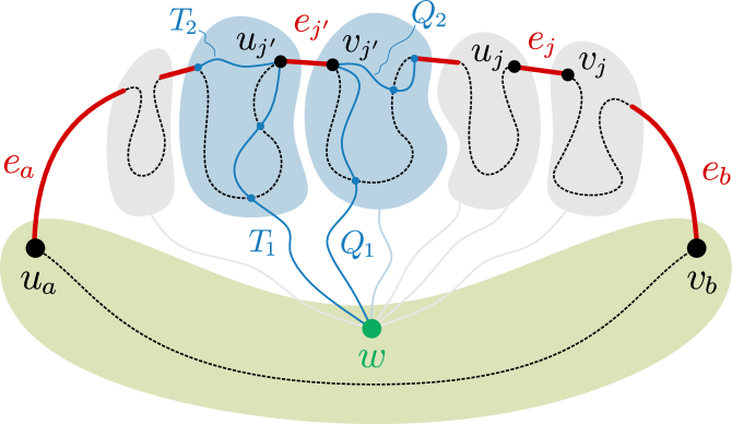
Figure 5. An illustration of the paths used in the proof of Lemma 4.35. The dashed lines represent the $u_{j}$-$v_{j}$ path $R$.

Lemma 4.35.

Let $G^{\prime},Z=\{e_{a},\dots,e_{b}\}$ be as above where $b\geqslant a+2k+3$. Let $j\in[a+1,b-1]$ be such that for every $f\in\{e_{a+1},\dots,e_{b-1}\}$, $w(f)\geqslant w(e_{j})$. Then, $e_{j}$ is irrelevant.

Proof 4.36.

In order to prove the lemma, we need to argue that if there is a solution for the instance $(G,k,w^{*},w,E^{\infty})$, then there is one which does not contain $e_{j}$. Let $S$ be a solution for this instance. If $S$ is disjoint from $e_{j}$, then we are done. Suppose that this is not the case. We first argue that there is an edge which is not in $S$ and has certain special properties. We will then argue that replacing $e_{j}$ with this special edge also leads to a solution for the same instance.

Claim 3.

There exists $j^{\prime}\in[a+1,b-1]$ such that $S$ is disjoint from $\Gamma[j^{\prime}-1,j^{\prime}]\cup\{e_{j^{\prime}}\}\cup\Gamma[j^{\prime},j^{\prime}+1]$.

Proof 4.37.

We first observe that $S$ is disjoint from $\{e_{a},\ldots,e_{b}\}\setminus\{e_{j}\}$ by Lemma 4.33. Next, for $\ell\in\{0,1,\dots,k\}$ let $\ell^{\prime}=a+2\ell$. Since there are $2k+2$ edges in the set $\{e_{a+1},\dots,e_{b-1}\}$ and by Observation 4.24, it follows that there are $k+1$ edge-disjoint sets $K_{1},\dots,K_{k+1}$ where

$$K_{\ell}=\Gamma[\ell^{\prime}+1,\ell^{\prime}+2]\quad\bigcup\quad\Gamma[\ell^{\prime}+2,\ell^{\prime}+3].$$

Since $|S|\leqslant k$, we conclude that there is an index $j^{\prime}$ such that $S$ is disjoint from $\Gamma[j^{\prime}-1,j^{\prime}]\cup\{e_{j^{\prime}}\}\cup\Gamma[j^{\prime},j^{\prime}+1]$. This completes the proof of the claim.

Furthermore, by our choice of $e_{j}$, it follows that $w(e_{j^{\prime}})\geqslant w(e_{j})$. Let $S^{\prime}=S\setminus\{e_{j}\}\cup\{e_{j^{\prime}}\}$. Clearly, $|S^{\prime}|\leqslant k$ and $w(S^{\prime})\geqslant w(S)$. We now argue that $S^{\prime}$ is also a biconnectivity deletion set.

Observe that in order to do so, it suffices to prove that there is a $u_{j^{\prime}}$-$v_{j^{\prime}}$ flow of value 2 in $G-S^{\prime}$. Let ${\cal Q}=\{Q_{1},Q_{2}\}$ be a $v_{j^{\prime}}$-$\{w,u_{j^{\prime}+1}\}$ flow of value 2 in the graph $G[{\sf Component}[j^{\prime},j^{\prime}+1]\cup\{w\}]$ where $Q_{1}$ is incident with $w$ and $Q_{2}$ with $u_{j^{\prime}+1}$ (see Figure 5). This flow exists by Lemma 4.31. Similarly, let ${\cal T}=\{T_{1},T_{2}\}$ be a $u_{j^{\prime}}$-$\{w,v_{j^{\prime}-1}\}$ flow of value 2 in the graph $G[{\sf Component}[j^{\prime}-1,j^{\prime}]\cup\{w\}]$ where $T_{1}$ is incident with $w$ and $T_{2}$ with $v_{j^{\prime}-1}$. By Observation 4.24, we know that ${\sf Component}[j^{\prime},j^{\prime}+1]$ and ${\sf Component}[j^{\prime}-1,j^{\prime}]$ are vertex-disjoint. Therefore, $J_{1}=Q_{1}+T_{1}$ is a $u_{j^{\prime}}$-$v_{j^{\prime}}$ path in $G-S^{\prime}$ and furthermore, $J_{1}$ is contained in $G[{\sf Component}[j^{\prime}-1,j^{\prime}]\cup{\sf Component}[j^{\prime},j^{\prime}+1]\cup\{w\}]$.

Since $S$ is a solution containing $e_{j}$, it follows that there is a $u_{j}$-$v_{j}$ flow of value 2 in the graph $G-S$. In particular, there is a $u_{j}$-$v_{j}$ path $R$ in the graph $G-S-w-e_{j}$. We assume without loss of generality that $j>j^{\prime}$. The arguments in the other case are exactly the same. Due to Lemma 4.33, we know that $R=R_{1}+R_{2}+R_{3}$ where the paths $R_{1}$, $R_{2}$ and $R_{3}$ satisfy the stated properties.

Let $R_{1}^{\prime}$ be the subpath of $R_{1}$ from $u_{j}$ to $u_{j^{\prime}+1}$, $R_{1}^{\prime\prime}$ be the subpath of $R_{1}$ from $v_{j^{\prime}-1}$ to $u_{a}$. Now, observe that $H=R_{1}^{\prime}+Q_{2}+e_{j^{\prime}}+T_{2}+R_{1}^{\prime\prime}+R_{2}+R_{3}$ is also a $u_{j}$-$v_{j}$ path in $G-S-w-e_{j}$. Futhermore, $H$ intersects $J_{1}$ only in $\{u_{j^{\prime}},v_{j^{\prime}}\}$.

Now, $C=H+e_{j}$ is a cycle in $G-S-w$ such that $S\cap E(C)=e_{j}$ and $S^{\prime}\cap E(C)=e_{j^{\prime}}$. Therefore, $J_{2}=C-e_{j^{\prime}}$ is a $u_{j^{\prime}}$-$v_{j^{\prime}}$ path in $G-S-w$. Since $C$ intersects $J_{1}$ only in $\{u_{j^{\prime}},v_{j^{\prime}}\}$, we conclude that $J_{2}$ is internally vertex-disjoint from $J_{1}$ and contains no edges of $S^{\prime}$. Thus, we have demonstrated a $u_{j^{\prime}}$-$v_{j^{\prime}}$ flow $\{J_{1},J_{2}\}$ of value 2 in the graph $G-S^{\prime}$, implying that $S^{\prime}$ is a biconnectivity deletion set and hence a solution for the instance $(G,k,w,w^{*},E^{\infty})$. Therefore, we conclude that the edge $e_{j}$ is irrelevant, completing the proof of the lemma.

Combining Lemma 4.19 and the fact that we can clearly locate the irrelevant edge $e_{j}$ (in the statement of Lemma 4.35) in polynomial time, we obtain Lemma 4.5, our main objective. This concludes the description of our algorithm for Weighted Biconnectivity Deletion.

4.3. A randomized kernel for Unweighted Biconnectivity Deletion

We now present our randomized kernel for the Weighted Biconnectivity Deletion problem where instances are of the form $(G,k,w^{*},w,E^{\infty})$ where $w(e)=1$ for every $e\in E(G)\setminus E^{\infty}$, $w(e)=0$ for every $e\in E^{\infty}$, and $w^{*}=k$. This version of the problem will be referred to as Unweighted Biconnectivity Deletion and instances of this problem will henceforth be of the form $(G,k,E^{\infty})$ where a solution is a biconnectivity deletion set of size $k$ contained in $E(G)\setminus E^{\infty}$. We continue to refer to the set $E(G)\setminus E^{\infty}$ as the set of potential solution edges and assume without loss of generality that at any point, any edge in the set ${\sf Critical}_{G}(\emptyset)$ is already part of $E^{\infty}$. Finally, recall that a linkage from $A$ to $B$ in a digraph $D$, where $A$ and $B$ are vertex sets, is a collection of $|A|=|B|$ pairwise vertex-disjoint paths originating in $A$ and terminating in $B$.

Our kernelization relies on a result of Kratsch and Wahlström [12]. Before we are able to state it formally, we need the following definitions. Let us define a potentially overlapping $A$-$B$ vertex cut in a digraph $D$ to be a set of vertices $C\subseteq V(D)$ such that $D-C$ contains no directed path from $A\setminus C$ to $B\setminus C$. For any digraph $D$ and set $X\subseteq V(D)$, a set $Z\subseteq V(D)$ is called a cut-covering set for $(D,X)$ if for any $A,B,R\subseteq X$, there is a minimum-cardinality potentially overlapping $A$-$B$ vertex cut $C$ in $D-R$ such that $C\subseteq Z$. We are now ready to state the result of Kratsch and Wahlström on which our kernelization is based.

Lemma 4.38 (Corollary 3, [12]).

Let $D$ be a directed graph and let $X\subseteq V(D)$. We can identify a cut-covering set $Z$ for $(D,X)$ of size $O(|X|^{3})$ in polynomial time with failure probability $O(2^{-|V(D)|})$.

Armed with this lemma, we first give a randomized kernelization that outputs an instance whose size is bounded polynomially in the number of the potential solution edges in the input instance.

Lemma 4.39.

Unweighted Biconnectivity Deletion has a randomized kernel with number of vertices bounded by $O(|E(G)\setminus E^{\infty}|^{3})$.

Proof 4.40.

Let $F=E(G)\setminus E^{\infty}$ be the set of potential solution edges. Now, the kernelization task essentially consists of retaining enough information from the input graph $G$ to verify for any set $S\subseteq F$, whether $S$ is a biconnectivity deletion set for $G$. Observe that this is equivalent to verifying whether there exists an edge $e=(u,v)\in S$, such that the maximum value of a $u$-$v$ flow in $G-S$ is less than 2. We show an equivalent formulation of this as a question about the existence of linkages in an auxiliary digraph, followed by an appropriate invocation of Lemma 4.38.

For the formulation, we create a digraph $D_{G,F}$ from $G$ and $F$. We refer to this digraph as $D$ when $G$ and $F$ are clear from the context. In the first step, subdivide every edge $e\in F$ with a new vertex $x_{e}$. That is, for an edge $e=(u,v)\in F$, we create a new vertex $x_{e}$, remove the edge $e$ and add edges $(u,x_{e})$ and $(v,x_{e})$. Let $G_{1}$ be the resulting undirected graph. In the second step, replace every edge $(u,v)$ in $E(G_{1})$ by a pair of arcs $(u,v)$, $(v,u)$. Finally, for every vertex $v$ incident to any edge of $F$ in $G$, add vertices $v^{+},v^{-}$ and add arcs from $v^{+}$ to all vertices in $N_{G_{1}}(v)$ and from all vertices in $N_{G_{1}}(v)$ to $v^{-}$. Let $D$ be the resulting digraph. Note that $N_{D}^{+}(v^{-})=\emptyset$ and $N_{D}^{-}(v^{+})=\emptyset$. Let $X_{E}=\{x_{e}\mid e\in F\}$, $X_{V}=\{v^{+},v^{-},v\mid e\in F,e=(u,v)\}$ and $X=X_{E}\cup X_{V}$. We now relate solutions for the given instance and linkages in $D$.

Claim 4.

For any $S\subseteq F$, $S$ is a biconnectivity deletion set for $G$ if and only if for every edge $(u,v)\in S$ there is a linkage from $\{u^{+},u\}$ to $\{v^{-},v\}$ in $D-\{x_{e}\mid e\in S\}$.

Proof 4.41.

Consider an arbitrary edge $e=(u,v)$ in $S$. On the one hand, assume that there exists a $u$-$v$ flow of value 2 in $G-S$. Then, by definition there exists a pair $\{P_{1},P_{2}\}$ of internally vertex-disjoint $u$-$v$-paths in $G-S$. Observe that orienting both paths from $u$ to $v$, replacing one copy of $u$ by $u^{+}$ and one copy of $v$ by $v^{-}$, and subdividing any edge $e^{\prime}\in E(P_{i})\cap F$ by the vertex $x_{e^{\prime}}$ yields the required linkage.

On the other hand, let $\{P_{1},P_{2}\}$ be a linkage from $\{u^{+},u\}$ to $\{v^{-},v\}$ in $D-\{x_{e}\mid e\in S\}$. For each $i\in\{1,2\}$, if $P_{i}$ originates in $u^{+}$, then replace $u^{+}$ by $u$ and if $P_{i}$ terminates in $v^{-}$, then replace $v^{-}$ by $v$. Call the paths resulting from $P_{1}$ and $P_{2}$ in this way, $P_{1}^{\prime}$ and $P_{2}^{\prime}$ respectively. Then $P_{1}^{\prime}$ and $P_{2}^{\prime}$ use only vertices of $V(G)\cup X_{E}$. Furthermore, these two paths use no edge of $S$ since by definition, $P_{1}$ and $P_{2}$ are disjoint from every vertex $x_{e^{\prime}}$ such that $e^{\prime}\in S$. Thus the paths $P_{1}^{\prime}$, $P_{2}^{\prime}$ use only edges and vertices present in $G-S$, and form an internally vertex-disjoint pair of $u$-$v$-paths.

Since the above applies to any edge, the claim follows.

Let $Z\subseteq V(D)$ be the cut-covering set for $(D,X)$, as computed by the algorithm of Lemma 4.38. Having in hand the set $Z$, we define the set $Y=(Z\cap V(G))\cup V(F)$. Note that $Z$ could contain vertices from $X_{V}$, but we want $Y$ to be a subset of $V(G)$. Therefore, we first add to $Y$ those vertices in $Z$ which are also vertices in $G$ and then add the vertices of $V(F)$. Our objective now is to reduce $G$ down to what is commonly known as the torso graph of $G$ defined by $Y$ (see [12]). We now make this precise in the form of reduction rules. In the rest of the proof of the lemma, we fix $Z$ to be a set computed using Lemma 4.38 and let $Y$ be as defined above. We now state three reduction rules which will be applied on the given instance in the order in which they are presented.

Reduction Rule 4.42.

If $k=0$, then return an arbitrary yes-instance of constant size.

Reduction Rule 4.43.

Suppose that Reduction Rule 4.42 has been applied on the given instance. If there is an edge $(u,v)\in F$ such that $G$ contains a $u$-$v$ path avoiding all edges of $F$ and all vertices of $Y\setminus\{u,v\}$, then delete $(u,v)$ from $G$ and reduce the budget $k$ by 1. That is, return the instance $(G-\{(u,v)\},k-1,E^{\infty})$.

Reduction Rule 4.44.

Suppose that Reduction Rule 4.42 and Reduction Rule 4.43 have been applied exhaustively on the given instance. For every pair $u,v\in Y$ such that $(u,v)\notin E(G)$ and there is a $u$-$v$-path in $G$ that is internally vertex-disjoint from $Y$, we add the edge $(u,v)$. Finally, return the instance $(G^{\prime},k,E^{\prime\infty})$, where $G^{\prime}=G[Y]$ and $E^{\prime\infty}=(E^{\infty}\cap E(G^{\prime}))\cup(E(G^{\prime})\setminus E(G))$.

The soundness of Rule 4.42 is trivial and we move on to prove the soundness of the remaining two rules.

Claim 5.

Reduction Rules 4.43 and 4.44 are sound.

Proof 4.45.

Let $e=(p,q)\in F$ be an edge which is deleted in an application of Reduction Rule 4.43. Observe that in order to argue the soundness of this reduction rule, it suffices to argue that $e$ is part of some solution for the given instance (if there exist any). Let $S$ be an arbitrary subset of $F$ containing $e$ such that $S\setminus\{e\}$ is a solution. If $S$ itself is a biconnectivity deletion set then we may correctly conclude that $e$ is part of some solution for the given instance. Suppose that this is not the case.

Recall that by the previous claim, $S$ is a biconnectivity deletion set for $G$ if and only if there is a linkage from $\{u^{+},u\}$ to $\{v^{-},v\}$ in $D-\{x_{e}\mid e\in S\}$ for every $(u,v)\in S$. Since we are in the case that $S$ is not a biconnectivity deletion set, there is a $(u,v)\in S$, with $A=\{u^{+},u\}$, $B=\{v^{-},v\}$, and $R=\{x_{e}\mid e\in S\}$ such that there is no linkage from $A$ to $B$ in $D-R$. Since $S\setminus\{e\}$ is a biconnectivity deletion set, we may assume without loss of generality that $u=p$ and $v=q$ and furthermore, $\kappa_{G-S}(p,q)=1$. In addition, the fact that $Z$ is a cut-covering set for $(D,X)$ implies that $Z$ contains a vertex $w$ such that $C=\{w\}$ is a minimum-cardinality potentially overlapping $A$-$B$ vertex cut in $D-R$. It is straightforward to see that $w\notin\{p,q,p^{+},q^{-}\}$ since otherwise, there will be at least one path from $A$ to $B$ which is disjoint from $w$. Finally, since $\kappa_{G-S}(p,q)=1$, it follows that every $p$-$q$ path in $G-S$ intersects $w$. If $w\in X_{E}$ then we know that it corresponds to an edge in $F$. Otherwise, it corresponds to a vertex in $Y$. In either case, we obtain a contradiction to the applicability of Reduction Rule 4.43 on the edge $(p,q)$, completing the proof of soundness for this rule.

We now argue the soundness of Reduction Rule 4.44. To do so, we prove that $S\subseteq F$ is a solution for $(G,k,E^{\infty})$ if and only if it is a solution for $(G^{\prime},k,E^{\prime\infty})$. Let $D_{1}=D_{G,F}$ and let $D_{2}=D_{G^{\prime},F}$.

In the forward direction, suppose that $S$ is a solution for $(G,k,E^{\infty})$. By Claim, 4, it follows that for every edge $(u,v)\in S$, there is a linkage from $\{u^{+},u\}$ to $\{v^{-},v\}$ in $D_{1}-\{x_{e}\mid e\in S\}$. Fix such an edge $(u,v)$ and let the paths in the linkage be $P_{1},P_{2}$. If we demonstrate such a linkage in $D_{2}$, then we are done. This can be achieved as follows. Let $i\in\{1,2\}$ and consider a pair of vertices $x_{i},y_{i}\in V(P_{i})\cap Y$ such that the subpath of $P_{i}$ from $x_{i}$ to $y_{i}$ has all its internal vertices disjoint from $Y$. Then, we know that the graph $G^{\prime}$ contains the edge $(x_{i},y_{i})$ and hence the digraph $D_{2}$ contains the arc $(x_{i},y_{i})$. We replace the subpath from $x_{i}$ to $y_{i}$ with the arc $(x_{i},y_{i})$ and we do this for every such subpath of $P_{i}$. It is straightforward to see that what results is indeed a linkage from $\{u^{+},u\}$ to $\{v^{-},v\}$ in $D_{2}-\{x_{e}\mid e\in S\}$. Hence, we conclude that $S$ is a solution for $(G^{\prime},k,E^{\prime\infty})$.

The same argument can be reversed for the converse direction in order to convert, for any $(u,v)\in S$, a linkage from $\{u^{+},u\}$ to $\{v^{-},v\}$ in $D_{2}-\{x_{e}\mid e\in S\}$ to a a linkage from $\{u^{+},u\}$ to $\{v^{-},v\}$ in $D_{1}-\{x_{e}\mid e\in S\}$. This completes the proof of soundness of Reduction Rule 4.44.

The above claim implies that if $(G^{\prime},k^{\prime},E(G^{\prime})\setminus F^{\prime})$ is the instance obtained by exhaustively applying the three reduction rules above, then $(G^{\prime},k^{\prime},E(G^{\prime})\setminus F^{\prime})$ is indeed equivalent to $(G,k,E^{\infty})$. Furthermore, the size $|V(G^{\prime})|=O(|F|^{3})$ and the randomized polynomial running time follow from Lemma 4.38. This completes the proof of the lemma.

See 1.3

Proof 4.46.

Let $(G,k,E^{\infty})$ be the given instance and let $F=E(G)\setminus E^{\infty}$ be the set of potential solution edges in this instance. We present reduction rules which reduce $F$ (while maintaining equivalence) to size $O(k^{3})$; the result then follows from Lemma 4.39.

If $|F|=O(k^{3})$, we are done. Otherwise, following the approach described in Section 4.2.1, we greedily construct a biconnectivity deletion set in $G$, at each step keeping track of the edges that become critical. That is, we let $\hat{S}=\{f_{1},\dots,f_{r}\}\subseteq F$ be a set greedily constructed as follows. The edge $f_{1}$ is an arbitrary edge in $F$ and for each $2\leqslant i\leqslant r$, $f_{i}$ is an arbitrary edge which is not critical in $G-\{f_{1},\dots,f_{i-1}\}$. As earlier, we terminate this procedure after $k$ steps if we manage to find edges $\{f_{1},\dots,f_{k}\}$ or earlier if for some $r<k$, every remaining edge of $F$ is critical in $G-\{f_{1},\dots,f_{r}\}$.

If $r=k$, then we identify the instance as a yes-instance and return an arbitrary yes-instance of constant size. Otherwise, if there is an $i\in[r]$ such that $G-\{f_{1},\dots,f_{i}\}$ is biconnected and $|{\sf Critical}_{G-\{f_{1},\dots,f_{i-1}\}}(f_{i})|\geqslant 20k^{2}+46k$, then we execute the case analysis in Section 4.2.2 and in polynomial time, either find $3k+1$ distinct partner sets or an irrelevant edge. In the latter case, we simply remove this irrelevant edge from $F$ (add it to the set $E^{\infty}$). Finally, if we reach a case with at least $3k+1$ distinct partner sets, then according to the proof of Lemma 4.19 we can find a biconnectivity deletion set $S\subseteq F$ with $|S|\geqslant k$ in polynomial time, and since we are dealing with the unweighted case, we can simply identify the instance as a yes-instance and return an arbitrary yes-instance of constant size.

The only remaining case is that this greedy algorithm fails to produce a large enough solution yet never marks too many edges as critical at once. That is, it terminates in $r<k$ steps and never marks more than $20k^{2}+46k$ edges as critical in step $i$ for any $i\in[r]$. This implies that $|F|\leqslant 20k^{3}+46k^{2}+k=O(k^{3})$, completing the proof of the theorem.

5. Conclusions

Our results on Path-contraction Preserving Strong Connectivity and Weighted Biconnectivity Deletion provide additional data points for the algorithmic landscape of graph editing problems under connectivity constraints and its application in network design.

Since we established that Path-contraction Preserving Strong Connectivity is W[1]-hard for general digraphs, we ask whether the problem becomes FPT when restricted to planar digraphs or other structurally sparse classes.

Concerning the parameterized algorithm for Weighted Biconnectivity Deletion, we ask whether the dependence of $2^{O(k\log k)}$ can be improved to single-exponential or proven to be optimal. Naturally, we would further like to know whether we can reach beyond biconnectivity and extend our algorithm to higher values of vertex-connectivity. Is it possible to obtain a similar algorithm on digraphs?

Finally, regarding our polynomial kernel for Unweighted Biconnectivity Deletion, we ask whether it is possible to obtain a deterministic kernel. It is also left open whether the weighted case admits a polynomial kernel.

The results presented in this paper raise more questions than they answer, a clear indication that connectivity constraints are far from properly explored under the paradigm of parameterized complexity. As such, the topic offers exciting but challenging opportunities for further research.

References

- [1] Jørgen Bang-Jensen and Gregory Z Gutin. Digraphs: theory, algorithms and applications. Springer Science & Business Media, 2008.
- [2] Jørgen Bang-Jensen and Anders Yeo. The minimum spanning strong subdigraph problem is fixed parameter tractable. Discrete Applied Mathematics, 156(15):2924–2929, 2008.
- [3] Manu Basavaraju, Fedor V Fomin, Petr Golovach, Pranabendu Misra, MS Ramanujan, and Saket Saurabh. Parameterized algorithms to preserve connectivity. In Proceedings of the 41st International Colloquium on Automata, Languages, and Programming (ICALP), pages 800–811. Springer, 2014.
- [4] Manu Basavaraju, Pranabendu Misra, M. S. Ramanujan, and Saket Saurabh. On finding highly connected spanning subgraphs. CoRR, abs/1701.02853, 2017.
- [5] Marek Cygan, Fedor V. Fomin, Lukasz Kowalik, Daniel Lokshtanov, Dániel Marx, Marcin Pilipczuk, Michal Pilipczuk, and Saket Saurabh. Parameterized Algorithms. Springer, 2015. URL: http://dx.doi.org/10.1007/978-3-319-21275-3, doi:10.1007/978-3-319-21275-3.
- [6] Fedor V. Fomin, Daniel Lokshtanov, Fahad Panolan, and Saket Saurabh. Efficient computation of representative families with applications in parameterized and exact algorithms. Journal of the ACM (JACM), 63(4):29:1–29:60, September 2016. URL: http://doi.acm.org/10.1145/2886094, doi:10.1145/2886094.
- [7] A. Frank. Connections in Combinatorial Optimization. Oxford Univ. Press, 2011.
- [8] András Frank. Augmenting graphs to meet edge-connectivity requirements. SIAM J. Discrete Math., 5(1):25–53, 1992.
- [9] András Frank and Tibor Jordán. Minimal edge-coverings of pairs of sets. J. Comb. Theory, Ser. B, 65(1):73–110, 1995.
- [10] Jiong Guo and Johannes Uhlmann. Kernelization and complexity results for connectivity augmentation problems. Networks, 56(2):131–142, 2010.
- [11] Stefan Kratsch. Recent developments in kernelization: A survey. Bulletin of the EATCS, 113, 2014. URL: http://eatcs.org/beatcs/index.php/beatcs/article/view/285.
- [12] Stefan Kratsch and Magnus Wahlström. Representative sets and irrelevant vertices: New tools for kernelization. In 53rd Annual IEEE Symposium on Foundations of Computer Science, FOCS 2012, New Brunswick, NJ, USA, October 20-23, 2012, pages 450–459. IEEE Computer Society, 2012. URL: http://dx.doi.org/10.1109/FOCS.2012.46, doi:10.1109/FOCS.2012.46.
- [13] Dániel Marx and László A Végh. Fixed-parameter algorithms for minimum-cost edge-connectivity augmentation. ACM Transactions on Algorithms (TALG), 11(4):27, 2015.
- [14] Dennis M Moyles and Gerald L Thompson. An algorithm for finding a minimum equivalent graph of a digraph. Journal of the ACM (JACM), 16(3):455–460, 1969.
- [15] Hiroshi Nagamochi. An approximation for finding a smallest 2-edge-connected subgraph containing a specified spanning tree. Discrete Applied Mathematics, 126(1):83 – 113, 2003. 5th Annual International Computing and combinatorics Conference. URL: http://www.sciencedirect.com/science/article/pii/S0166218X02002184, doi:http://dx.doi.org/10.1016/S0166-218X(02)00218-4.
- [16] László A. Végh. Augmenting undirected node-connectivity by one. SIAM J. Discrete Math., 25(2):695–718, 2011.
- [17] T. Watanabe and A. Nakamura. Edge-connectivity augmentation problems. J. Comput. System Sci., 35:96 – 144, 1987.