Context-based Object Viewpoint Estimation:
A 2D Relational Approach

Abstract

The task of object viewpoint estimation has been a challenge since the early days of computer vision. To estimate the viewpoint (or pose) of an object, people have mostly looked at object intrinsic features, such as shape or appearance. Surprisingly, informative features provided by other, extrinsic elements in the scene, have so far mostly been ignored. At the same time, contextual cues have been proven to be of great benefit for related tasks such as object detection or action recognition. In this paper, we explore how information from other objects in the scene can be exploited for viewpoint estimation. In particular, we look at object configurations by following a relational neighbor-based approach for reasoning about object relations. We show that, starting from noisy object detections and viewpoint estimates, exploiting the estimated viewpoint and location of other objects in the scene can lead to improved object viewpoint predictions. Experiments on the KITTI dataset demonstrate that object configurations can indeed be used as a complementary cue to appearance-based viewpoint estimation. Our analysis reveals that the proposed context-based method can improve object viewpoint estimation by reducing specific types of viewpoint estimation errors commonly made by methods that only consider local information. Moreover, considering contextual information produces superior performance in scenes where a high number of object instances occur. Finally, our results suggest that, following a cautious relational neighbor formulation brings improvements over its aggressive counterpart for the task of object viewpoint estimation.

1 Introduction

During the last decade, contextual information has proven beneficial for vision tasks such as image segmentation and object detection. For the task of object detection, there is a significant amount of work, e.g. [2, 8, 9, 11, 20, 49, 56], in which pairwise relations between object hypotheses are exploited to re-rank the initial predictions given by the object detector. Following a different direction, a more recent group of works [1, 45, 50] has focused on exploiting contextual information to iteratively generate object proposals during test time and improve object detection. Likewise, for image segmentation [6, 24, 60], context is considered by analyzing appearance and spatial co-occurrence of neighboring segments and is used to enforce spatial consistency. However, despite the demonstrated benefits for the already mentioned tasks, contextual information has been mostly ignored for the task of object viewpoint or pose estimation. Only recently, [43], [64] and [66] took initial steps towards exploiting contextual information for predicting the viewpoint/pose of a group of objects.

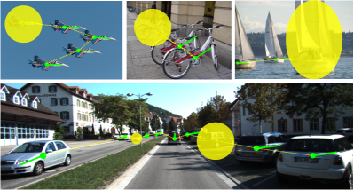
Figure 1: The natural or “desired” configurations in which objects occur in the world often provide strong cues of their viewpoint. For instance, it is not difficult to guess the viewpoint of the objects behind the yellow regions by only looking at the other objects in the scene.

Here, we follow the line of our earlier work [43] and exploit pairwise relations between objects as a source of contextual information for estimating the viewpoint of each of the objects. Let us clarify the intuition behind this work with the following example: imagine you are given the task of predicting the viewpoint of the objects below the yellow regions in Figure 1. Even when there is no access to intrinsic features of the objects such as color or texture, the overall configuration of surrounding objects provides a strong cue to predict their viewpoint. This can be considered a Collective Classification problem [46, 54], in which the class (viewpoint) of one object influences that of another (see Figure 2). Collective classification is a popular problem in machine learning and data mining, in which the data takes the form of a graph and the task is to predict the classes of the nodes in the graph while using the structure of the network and a few example classifications of nodes. See Algorithm 1 for a brief description of Collective Classification [46].

A common practice [36, 38, 62] in Collective Classification [46] when reasoning about relations between objects is that, during inference, the neighboring object hypotheses are considered without taking into account the certainty of their prediction. As a result, all the neighbors participate in and contribute equally to the classification of each object. Following the literature [39, 40] on Collective Classification, instead, we propose an iterative scheme where we first classify the viewpoints of objects with the most certain relational information, and then use these to bootstrap the predictions of the other objects. This is useful in collective classification tasks, like object detection or object viewpoint estimation, where multiple possibly related objects all need to be classified (see Figure 1). Following the terminology of [39], we refer to these two inference variants as “aggressive” inference, where all the neighboring objects are considered as sources of contextual information, and “cautious” inference, where we iteratively select the objects with highest certainty as source of contextual information. In this paper, we empirically evaluate the added value of aggressive vs. cautious inference for the task of object viewpoint estimation.

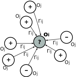
Figure 2: Collective Classification. We address the classification of a particular object $o_{i}$ (in gray) based on the relations $r_{ij}$ with its neighboring objects $o_{j}$.

Algorithm 1 Collective Classification [46]

Given

• A set of interrelated nodes $o_{i}$ connected by links $r_{ij}$.

Steps

1. Local Classification: classify each of the nodes $o_{i}$ using the non-relational (local) model. This model focuses purely on attributes of the nodes.

2. Relational Classification: classify each of the nodes $o_{i}$ using the relational classifier which takes into account neighboring nodes $o_{j}\in N_{i}$ connected via links $r_{ij}$.

3. Collective Inference: re-classify the nodes $o_{i}$ together, taking into account the classification output obtained in steps 1 and 2, and possibly iterate.

This paper complements our earlier work [43] in two ways: first, by providing a more elaborate theoretical treatment of the method, and second, by providing a wider experimental validation, including an evaluation with a larger set of detectors, and a deeper analysis of success and failure cases. Moreover, in order to generalize to images where extracting 3D information might be too complex, in the present paper we focus on 2D spatial relations instead of relations in the 3D space.

This paper is organized as follows: Section 2 presents related work. Section 3 shows how we define and learn relations between objects in the scene and how we combine the contextual response provided by the related objects with the evidence from local detectors. Implementation details are presented in Section 4. Then, Section 5 describes our evaluation protocol and the obtained results and discussions. Limitations and directions for future work are presented in Section 6. Finally, we draw conclusions in Section 7.

2 Related Work

The task of object viewpoint estimation can be analyzed from different perspectives. In this work we focus on four aspects that will help position our work: the cues used for viewpoint estimation, sources of contextual information, how inference between objects is performed and by comparing our work w.r.t. holistic scene understanding.

2.1 Cues for object viewpoint estimation

Several object viewpoint estimation methods have been proposed in the literature. Most of these rely on intrinsic characteristics of the object category such as color, texture or gradient patterns. In the traditional processing pipeline for object viewpoint estimation, first, candidate regions to host object instances are proposed. Secondly, an appearance descriptor is computed in the area of each candidate region. Finally, based on a pre-trained model, each descriptor is classified as one of the possible viewpoints the object may take. Following this pipeline, methods have evolved from modeling the appearance of 2D views that the objects may take under different viewpoints (e.g. [19, 32, 63]) to reasoning about geometric configurations of parts of the objects in the 3D space [22, 31, 47, 53]. Recently, several works [18, 26, 55, 57] have demonstrated the benefits of using learning-based representations to model object appearance and perform viewpoint estimation. In [18], it was shown that the activations of the last hidden layer of a pretrained convolutional neural network (CNN) can effectively serve as features to describe object viewpoints. Moreover, these learned features outperform methods that rely on traditional 2D features and features derived from 3D models. In [55], two CNN architectures are proposed, first, to coarsely estimate the viewpoint of the object, and second, to refine the predicted viewpoint by focusing on keypoints. In [26] a compact model is proposed where image features extracted by the detector are shared with the viewpoint estimator with the objective of achieving real-time performance. Finally, [57] generates synthetic images from 3D object collections to render a high volume of images with high variation which can be exploited by a CNN. In our earlier work [43], we explored an “allocentric” approach in which the 3D pose of an object influences that of another. In that formulation, pairwise relations between objects in the 3D space were considered as sources of contextual information. To this end, a pair of local and contextual responses were computed for each object in the scene. On the local side, the output of a viewpoint-aware object detector, namely [17] and [32], was used. On the contextual side, the weighted sum of the belief of each of the contextual objects was computed following a weighted-vote relational classifier [38]. Then, these responses were combined to produce a final pose prediction. Following this approach it was shown that considering contextual cues brings improvements to the estimation of object poses. Parallel to this, [64] proposed a method that reasons about intrinsic features from the objects such as the appearance of patches taken from the object, and contextual cues such as 2D occlusion of other objects, to estimate the location and viewpoint of the objects in the scene. Based on these components, [64] proposed a spatial layout model that enforced scene consistency based on the 3D aspectlets of individual objects with object-object consistency in the form of occlusion reasoning. Similarly, [66] used a fine detail shape representation based on CAD models. This representation improved model-object matching in the scene and, as consequence, better reasoning about object support on the ground-plane and mutual occlusion between objects. In this work we follow this line of work. We further explore the allocentric approach from [43] where the object viewpoint estimation task is formulated as a collective classification problem. However, different from [43], we focus on the prediction of the viewpoint, i.e. the projected orientation of the object that is observed by the camera, rather than the 3D pose (azimuth angle) of objects in the 3D scene. Different from [66] and [57] we will limit our training procedure to focus on manually annotated images and not look into the use of synthetic data. Furthermore, our method operates in still images and does not require image sequences as in some SfM-based approaches [3, 4].

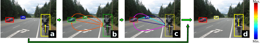
Figure 3: Algorithm Pipeline: a) viewpoint-aware object detection (score encoded in jet scale), b) pairwise relations definition, c) object contextual scoring via wvRN classifier [38], and d) combination of local and contextual responses. During the contextual scoring step (c), the relations that are used to compute the contextual score of each object are grouped by color.

2.2 Sources of contextual information

Scene elements have been defined in several ways; [15] proposes that some objects have a defined shape or appearance while others can be characterized by their color or texture. Following these definitions [15] divided such elements as Things and Stuff, respectively. Both types of elements have been used in the past as sources of contextual information. However, in this paper we will focus on Things. Using this type of element, [11] defined a template on top of the bounding boxes covering the objects. Then, these templates were used to extract discrete spatial relations, such as on-top, next-to, below, near, far, between object hypotheses. In that work, using other objects as context proved to be helpful to possibly identify and degrade false hypotheses bringing improvements on object detection performance. Following this trend, Felzenszwalb et al. [13], Perko & Leonardis [49] and Choi et al. [8] addressed a similar problem with the difference that they defined continuous spatial relations instead of discrete ones. These continuous relations were extracted by estimating the difference between the centers of object bounding boxes. Finally, the learned relations were used to filter out the out-of-context objects. [56] suggested a joint detection-classification scheme to identify ambiguously scored hypotheses and used an adaptive method to exploit context information on these hypotheses. In [9] relations between objects extended the traditional approach of exploiting object co-occurrences and considered additional features such as relative scales, bounding box overlap ratio and scores. Furthermore through a set-based formulation this method has been shown able to reason about object spatial configurations that go beyond pairwise interactions. Similar to these works, we exploit relations between Things as sources of contextual information. However, we will focus on the task of estimating the viewpoint of each object.

2.3 How inference between objects is performed

From the perspective of the Collective Classification literature [46], specifically on the inference side, our method is inspired by Cautious Inference [40, 42]. This is a type of inference that seeks to identify and exploit the more certain relational information. Such a cautious approach was used in [24] for labeling object superpixels. In [24], discriminative relations were mined between object regions and discriminative attributes were discovered per relation. In [44], relations between objects were considered to improve object detection by penalizing out-of-context object hypotheses. During inference, the object hypotheses with highest certainty are classified first and then used to bootstrap the other objects. Based on their experiments, it was concluded that all cases following this cautious iterative approach resulted in better object detection performance than when considering all the neighboring objects at once. In this work, we start from the observations of [44], and explore a cautious counterpart of [43] with the objective of verifying whether the observations made for object detection also hold for the task of object viewpoint estimation. To this end, we first estimate the viewpoint of the objects with higher certainty and then use these objects to predict the viewpoints of the other ones.

To some extent, the proposed method bears some resemblance to the message-passing algorithms [65] commonly used for inference in graphical models. In the same fashion as the message-passing algorithms, we start from input elements for which information is available, in this case the objects that define the nodes in the graph. Then, we iteratively select a target node, in our case each of the object hypotheses to be re-estimated, and each of the neighboring nodes (objects) casts a vote (or sends a message) indicating the level of agreement they have with the target node taking a specific state. Furthermore, similar to message-passing algorithms, for the case of loopy graphs the proposed method aims at providing an approximate solution to the problem at a relative low computation time. Different from message-passing algorithms, which operate over a graph defined over two types of nodes (variable nodes and check nodes), our method only considers variable nodes.

2.4 Towards holistic scene understanding

In the literature there is a group of works [14, 21, 27, 30, 58] that study the problem of holistic scene understanding. This problem consists of jointly reasoning about regions, location, category and spatial extent of objects in the image, as well as the scene type. The main idea behind holistic scene understanding is that all these problems, traditionally addressed in isolation, complement each other and this complementarity can assist to improve each individual task. Related works that follow these characteristics are [64] and [66]. These works propose methods that, as part of their pipeline, reason about object viewpoints/poses. In [64], a Spatial Layout Model that jointly reasons about inter object occlusions, rough 3D shape of the objects and scene ground-plane is proposed. In addition, 2D regions partially covering the objects are grouped producing “3D aspectlets”. The method proposed in [66] reasons about fine-detailed 3D shape of the objects while reasoning about object occlusions and scene ground-plane contact. Different from the approaches addressing the more general problem of holistic scene understanding, our approach is more specific in the sense that it focuses purely on reasoning about relations between objects, i.e. Things entities. Particularly, in comparison with [64] and [66] which relate objects as means to model occlusions, in our work relations between objects are aimed at modeling usual configurations in which the objects of interest occur. Our method represents a more semantic relational layer between objects that could be integrated in current methods aiming at holistic scene understanding.

3 Proposed Method

This work is based on our previous work [43]. While in [43] we reasoned about locations and poses of objects in the 3D scene, here we shift the feature extraction and reasoning to the 2D image space. We assume that some features of an object, in this case its 2D location and viewpoint, are not only influenced by the object itself but somehow driven by other entities in the scene. This idea is inspired by the concept of “Allocentrism”, a term in Psychology used to define entities that tend to be interdependent, defining themselves in terms of the group they are part of, and behaving according to the norms of the group [23, 61]. Allocentric entities appear to see themselves as an extension of their group. Based on this description, our method takes into account the group consistency of each entity relative to the group defined by the other entities in the scene.

The proposed method consists of four steps (see Algorithm 2): First, given an image, we run an off-the-shelf viewpoint-aware object detector to collect a set of object hypotheses with class label and predicted discrete viewpoint (Figure 3(a)). Then, we define pairwise relations between all the object hypotheses (Figure 3(b)). Third, for each of the object hypotheses, we estimate its contextual response using as source of contextual information the other object hypotheses (see Figure 3(c)). Finally, we combine the local response, provided by the viewpoint-aware object detector, with the contextual response to obtain the final viewpoint estimate (Figure 3(d)). Now we will present a more detailed description of the proposed method.

Algorithm 2 Proposed Method

Given

• viewpoint-aware object detector.

• Image $I$.

Steps

1. Collect object hypotheses $\{o_{i}\}$ with local confidences $\psi^{l}_{i}$ from $I$ using a viewpoint-aware detector.

For each object hypothesis $o_{i}$:

1. Define pairwise relations with the other hypotheses $o_{j}$ in its context $N_{i}$ ($o_{j}$ are neighboring objects of $o_{i}$).

2. Compute its contextual response $\psi^{c}_{i}=wvRN(o_{i}|N_{i})$ via wvRN [38] using objects $o_{j}\in N_{i}$. (see section 3.2)

3. Combine the local confidence $(\psi^{l}_{i})$ and contextual response $(\psi^{c}_{i})$ to predict the object viewpoint.

3.1 Object Relations as Source of Context

Before we discuss how relations between objects can be used as a source of contextual information, we introduce the representations for objects and relations used in this paper. Given an image, we use a viewpoint-aware object detector to collect a set of object hypotheses $O=\{o_{1},o_{2},...,o_{m}\}$ of the categories of interest. Each object hypothesis $o_{i}$ is represented as a tuple $o_{i}=(c_{i},l_{i},f_{i},s_{i})$ where $c_{i}$ represents the category of the object, $l_{i}$ represents the location of the center of the bounding box of the object in the scene, $f_{i}$ represents additional object-related features (e.g. aspect ratio or scale), and $s_{i}$ the local detection score reported by the detector. In addition, each hypothesis is accompanied with a predicted discrete viewpoint $\alpha_{i}$. We will use the superscript variable $\upsilon$ on $o^{\upsilon}$ to indicate the state of the predicted object hypothesis. We refer with $o^{+}$ to the object hypotheses that are correctly localized, i.e. their predicted bounding boxes cover valid object instances. We will refer with $o^{-}$ to false object hypotheses. Similarly, We use the superscript variable $\omega$ on $\alpha^{\omega}$ to indicate the state of the predicted viewpoint. We use $\alpha^{+}$ and $\alpha^{-}$ to indicate whether the viewpoint $\alpha$ of the object is predicted correctly or not. Finally, we will use the shorthand $\overline{\alpha}^{\omega}$ to combine the predicted viewpoint class and its state, i.e. $\overline{\alpha}^{\omega}=(\alpha,\alpha^{\omega})$.

To measure the level to which an object fits in a group of objects, we need to define a set of relations $R=\{r_{ij}\}$ between objects. Here, we limit ourselves to pairwise relations. We define these relations as the relative values between the attributes of the 2D bounding boxes of objects in the scene. Given the set of object hypotheses $O$, for each object $o_{i}$ we define pairwise relations $r_{ij}$ with each object $o_{j}$ in its neighborhood $N_{i}$. For simplicity, we set $N_{i}$ equal to the set composed by every other object in the image. This produces a total of $(m(m-1))$ pairwise relations per image (See Figure 2 and 3(c)) with $m$ the total number of objects in the image. In Section 4 we describe how we compute the attributes that define the relations $r_{ij}$.

We summarize the notations in the following table:

Variable	Description
$o_{i}=(c_{i},s_{i},f_{i},l_{i})$	Object hypothesis.
$o^{\upsilon}_{i}$	Denotes whether the object hypothesis $o_{i}$ is true or false, $\upsilon\in(+,-)$
$\alpha_{i}$	Denotes the predicted viewpoint
$\alpha^{\omega}_{i}$	Denotes whether $\alpha_{i}$ is correct or not, $\omega\in(+,-)$
$\overline{\alpha}^{\omega}_{i}=(\alpha_{i},\alpha^{\omega}_{i})$	Shorthand
$r_{ij}$	Relational feature computed from $(f_{i},l_{i})$ and $(f_{j},l_{j})$.

Table 1: Notation summary

3.1.1 Measuring Contextual Support between Objects

The problem we’re addressing can be seen as a Collective Classification problem in which the class (viewpoint) of an object influences that of another. We follow a simple three-step collective classification approach (see Alg.1) as proposed in [38]. In order to take into account the relations between objects, we estimate a response for each object $o_{i}$ based on the relations with all the objects $o_{j}$ in its context. This contextual response is obtained using the weighted-vote Relational Neighbor classifier (wvRN) [38]. This relational classifier, formally known as the probabilistic Relational Neighbor classifier (pRN) [36], is a simple, yet powerful classifier that is able to take advantage of the underlying structure between networked data. It operates in a node-centric fashion, that is, it processes one object $o_{i}$ at a time based on the objects $o_{j}$ in its context. During the last decade, wvRN has been successfully applied in work related to text mining [36, 38], web-analysis [38], suspicion scoring [37], link prediction [33], and social network analysis [34, 35]. More recently we applied it in the computer vision field to address the task of context-based object pose estimation [43] and context-based object detection [44]. The wvRN classifier [38] computes a contextual score in general, as follows:

$$wvRN(o_{i}|N_{i})=\frac{1}{Z}\sum_{o_{j}\in N_{i}}v(o_{i},o_{j}).w_{j}\\$$ (1)

newith $Z=\sum w_{j}$ a normalization term, $v(o_{i},o_{j})$ a pairwise term measuring the likelihood of object $o_{i}$ given its relation with object $o_{j}$, and the weighting factor $w_{j}$ modulating the effect of the neighbor $o_{j}$. In this paper we are interested in the prediction of the viewpoint $\alpha_{i}$ of each object hypothesis $o_{i}$. We stress this by explicitly adding the viewpoint $\alpha_{i}$ in the equations. In addition, we apply the notation introduced earlier. As a result, the argument of Eq. 1 is redefined as:

$$wvRN(o_{i}|N_{i})=wvRN(\alpha_{i}^{+},o_{i}^{+}|N_{i})$$ (2)

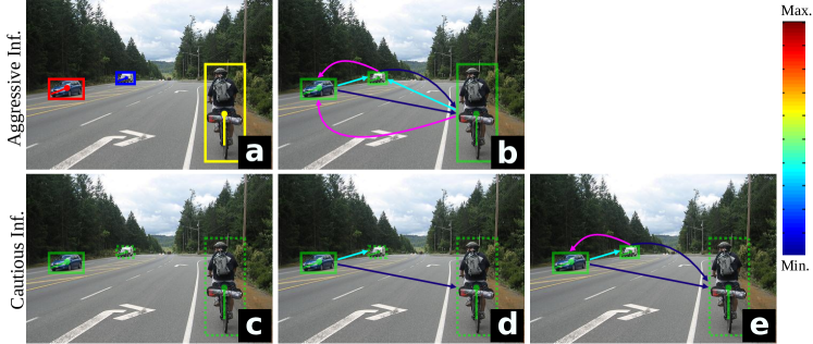
Figure 4: Types of relational inference. a) Viewpoint-aware object detection hypotheses (score encoded in jet scale), b) Aggressive inference, and c-e) Cautious inference. Influence of an object over another is indicated by the arrows. Solid for known objects, dashed boxes for object hypotheses to be classified. Notice how the final graph topology between b) and e) differs depending on the type of inference used.

3.2 Context-based Viewpoint Classification

Given an image with a set of 2D objects $o=\{o_{1},...,o_{m}\}$, we estimate the viewpoint $\alpha_{i}$ of an object $o_{i}$ as the viewpoint $\hat{\alpha_{i}}$ that maximizes the likelihood of object $o_{i}$ given its neighborhood $N_{i}$:

$$\hat{\alpha_{i}}=\arg\max_{\alpha_{i}}(~{}wvRN(\overline{\alpha_{i}}^{+},o_{i}^{+}|N_{i})~{}),\\$$ (3)

As mentioned earlier, the group fitting of an object is measured by the output of the wvRN classifier [38] which is defined, for our specific task, as follows:

$$wvRN(\overline{\alpha_{i}}^{+},o_{i}^{+}|N_{i})=\frac{1}{Z}\sum_{o_{j}\in N_{i}}p(\overline{\alpha_{i}}^{+},o_{i}^{+}|r_{ij},c_{i})\cdot w_{j}\\$$ (4)

In our formulation $w_{j}$ is a weighting term that takes into account the noise in the object detector (see below). The original pairwise term $v(o_{i},o_{j})$ is defined as $p(\overline{\alpha_{i}}^{+},o_{i}^{+}|r_{ij},c_{i})$. This conditional represents the probability of object $o_{i}$, of category $c_{i}$, being a true hypothesis $o_{i}^{+}$, with correctly predicted viewpoint $\overline{\alpha_{i}}^{+}$, given its relation $r_{ij}$ with object $o_{j}$. Using Bayes’ Rule we estimate $p(\overline{\alpha_{i}}^{+},o_{i}^{+}|r_{ij},c_{i})$ as the posterior:

$$p(\overline{\alpha}_{i}^{+},o_{i}^{+}|r_{ij},c_{i})=\frac{p(r_{ij}|\overline{\alpha}_{i}^{+},o^{+}_{i},c_{i})p(\overline{\alpha}_{i}^{+},o^{+}_{i}|c_{i})}{p(r_{ij}|c_{i})}\\ \\ =\frac{p(r_{ij}|\overline{\alpha}_{i}^{+},o^{+}_{i},c_{i})p(\overline{\alpha}_{i}^{+},o^{+}_{i}|c_{i})}{\sum\limits_{\upsilon~{}\in~{}\{+,-\}}\sum\limits_{\omega~{}\in~{}\{+,-\}}~{}p(r_{ij},\overline{\alpha}_{i}^{\omega},o^{\upsilon}_{i}|c_{i})}\\ \\ =\frac{p(r_{ij}|\overline{\alpha}_{i}^{+},o^{+}_{i},c_{i})p(\overline{\alpha}_{i}^{+},o^{+}_{i}|c_{i})}{\sum\limits_{\upsilon~{}\in~{}\{+,-\}}\sum\limits_{\omega~{}\in~{}\{+,-\}}~{}p(r_{ij}|\overline{\alpha}^{\omega}_{i},o^{\upsilon}_{i},c_{i})p(\overline{\alpha}^{\omega}_{i},o^{\upsilon}_{i}|c_{i})}$$ (5)

The components of Eq.5 are obtained through the following procedure. During the training stage, we compute pairwise relations $r_{ij}$ between the annotated objects in the training images. Furthermore, we extend this set of objects and relations by running a local detector on the training set producing a set of hypotheses per image. Then, we flag the hypotheses as true positive hypotheses $o_{i}^{+}$ or as false positive hypotheses $o_{i}^{-}$ considering spatial matching based on the Pascal VOC [12] matching criterion. In addition, each object hypothesis is flagged as $\overline{\alpha}_{i}^{+}$ or $\overline{\alpha}_{i}^{-}$ depending on whether its viewpoint was predicted correctly or not, respectively. Note that hypotheses with label combination $(\overline{\alpha}_{i}^{+},o_{i}^{-})$ do not exist since it is not possible to predict correctly the viewpoint of a false hypothesis. In order to avoid repeated object instances, we replace true hypotheses $o_{i}^{+}$, with correctly predicted viewpoint $\overline{\alpha}_{i}^{+}$, by their corresponding annotations. Similarly, we replace the relations produced by these correct hypotheses by those produced by their corresponding annotations. This step of integrating the hypotheses in the training data, allows our method to model, up to some level, the noise in the relations $r_{ij}$ introduced by the local detector. More specifically, this noise appears in the form of frequent false relations that arise from common false hypotheses that may be predicted by the local detector. This produces a set of objects $o_{i}$ with their corresponding pairwise relations $R=\{r_{ij}\}$ from the whole training set. Using this information, we estimate a probability density function (pdf) via Kernel Density Estimation (KDE). Finally, during testing, $p(r_{ij}|\overline{\alpha}_{i}^{+},o^{+}_{i},c_{i})$, $p(r_{ij}|\overline{\alpha}_{i}^{-},o_{i}^{+},c_{i})$ and $p(r_{ij}|\overline{\alpha}_{i}^{-},o_{i}^{-},c_{i})$ are computed by evaluating the pdf at the test points defined by the relations $r_{ij}$ computed between object hypotheses.

This method captures the statistics of typical configurations. The priors $p(\overline{\alpha}_{i}^{+},o_{i}^{+}|c_{i})$, $p(\overline{\alpha}_{i}^{-},o_{i}^{+}|c_{i})$ and $p(\overline{\alpha}_{i}^{-},o_{i}^{-}|c_{i})$ are estimated per object category based on their occurrence in the training set, respectively. Moreover, given that hypotheses with label combination $(\overline{\alpha}_{i}^{+},o_{i}^{-})$ do not exist, we set the prior $p(\overline{\alpha}_{i}^{+},o_{i}^{-}|c_{i})=0$. Note that the conditional terms $p(r_{ij}|\overline{\alpha}^{\omega}_{i},o^{\upsilon}_{i},c_{i})$ are derived from a distribution representing the relational space covering pairwise relations from specific object categories. For this reason, in order to consider relations between objects of different categories, during training, we estimate the pdfs from pairwise relations (samples) with a specific object category, as source, and a specific object category, as target. Given a set of $n$ object categories of interest, we model a total of $n^{2}$ pdfs that will be used later to compute the term $p(r_{ij}|\overline{\alpha}^{\omega}_{i},o^{\upsilon}_{i},c_{i})$.

The weighting factor $w_{j}$ of Eq. 4 takes into account the noise that is introduced by the object detector in the predicted neighboring objects $o_{j}$. We estimate $w_{j}$ using a Probabilistic Local Classifier that takes into account the score $s_{j}$ provided by the object detector for its respective hypothesis $o_{j}$. The output of this classifier will be the posterior $p(\overline{\alpha}_{j}^{+},o_{j}^{+}|s_{j},c_{j})$ of object $o_{j}$ of category $c_{j}$ being correctly localized ($o_{j}^{+}$), with correctly predicted viewpoint $\overline{\alpha}_{j}^{+}$, given its score $s_{j}$. We compute this posterior following the procedure presented in [49]:

$$w_{j} =p(\overline{\alpha_{j}}^{+},o^{+}_{j}|s_{j},c_{j})$$ (6)

$$=\frac{p(s_{j}|\overline{\alpha_{j}}^{+},o^{+}_{j},c_{j})p(\overline{\alpha_{j}}^{+},o^{+}_{j}|c_{j})}{\sum\limits_{\upsilon~{}\in~{}\{+,-\}}\sum\limits_{\omega~{}\in~{}\{+,-\}}~{}p(s_{j}|\overline{\alpha}^{\omega}_{j},o^{\upsilon}_{j},c_{j})p(\overline{\alpha}^{\omega}_{j},o^{\upsilon}_{j}|c_{j})}$$

The components of this equation are obtained following a procedure similar to that for Eq. 5 up to the point where hypotheses are assigned the labels $\overline{\alpha}^{+}$, $\overline{\alpha}^{-}$, $o^{+}$ and $o^{-}$. Then, based on these flagged hypotheses, we compute the conditionals $p(s|\overline{\alpha}^{+},o^{+},c)$, $p(s|\overline{\alpha}^{-},o^{+},c)$ and $p(s|\overline{\alpha}^{-},o^{-},c)$ respectively via KDE. Finally, the priors $p(\overline{\alpha}^{+},o^{+}|c)$, $p(\overline{\alpha}^{-},o^{+}|c)$ and $p(\overline{\alpha}^{-},o^{-}|c)$ are estimated per category as the corresponding proportions of labeled hypotheses in the training data. As a result, $p(\overline{\alpha}_{j}^{+},o_{j}^{+}|s_{j},c_{j})$ expresses the probability of a hypothesis being correct given its detection score. This procedure allows us to plug-in any standard object detector in our method. Note that, similar to the term $p(r_{ij}|\overline{\alpha}_{i}^{+},o^{+}_{i},c_{i})$, the conditional $p(s|\overline{\alpha}^{+},o^{+},c)$ is computed from object category-wise KDE, where all the sample points are derived from object hypotheses belonging to the object category of interest.

3.3 Cautious Inference

Following the definition introduced in [39], an algorithm is considered “cautious” if it seeks to identify and employ the more certain or reliable relational information. We focus on two factors that [39] introduced to control the degree of caution in an algorithm. The first factor dictates to use only objects for which the prediction is confident enough. The second factor increases caution by favoring already-known relations. These are relations that have been seen in the training images.

For the aggressive version of our relational classifier, we use wvRN as described in Eq. 4. For each object hypothesis to be classified, it considers all the other objects $o_{j}$ in its context $N_{i}$ during the inference (see Figure 4(b)). For the cautious version of our relational classifier, we enforce the above principles in the following fashion.

For the first principle, giving relevance to the most-certain objects, we perform an iterative approach inspired by [42]. Given a set of hypotheses $O=\{o_{1},...,o_{n}\}$, we define the disjoint sets $O^{k}$ and $O^{u}$ containing the known and unknown objects, respectively, with $O=O^{k}\cup O^{u}$ at all times. During inference, we initialize $O^{k}=\{\}$ and $O^{u}=O$ and flag as known object, the hypothesis with the highest score based on the probabilistic local classifier (Eq. 6) . This hypothesis is moved to the set of known objects $O^{k}$. Then, the wvRN score for each of the unknown objects $o_{i}\in O^{u}$ is re-estimated considering only the known objects $o_{j}\in O^{k}$ in their context $N_{i}$. This redefines Eq. 4 in the following way:

$$wvRN(\overline{\alpha}_{i}^{+},o^{+}_{i}|N_{i})=\frac{1}{Z}\sum_{\mathclap{~{}o_{j}\in(N_{i}\cap O^{k})}}p(\overline{\alpha}_{i}^{+},o^{+}_{i}|r_{ij},c_{i})\cdot w_{j}\\$$ (7)

We flag the hypothesis with highest wvRN response as known and move it to the set of known objects $O^{k}$. We repeat this procedure promoting one hypothesis $o_{i}\in O^{u}$ at a time until the set of unknown objects $O^{u}$ is empty. Finally, for the sake of similarity in the ranking of the new scores, we re-estimate the score of the first promoted object using Eq. 7 with the second promoted object as known contextual object.

For the second principle of cautious inference: “favoring relations already seen on training data”, our use of KDE for estimating the vote $p(\overline{\alpha}_{i}^{+},o^{+}_{i}|r_{ij},c_{i})$ from each contextual object $o_{j}$ implicitly introduces this characteristic in the inference.

For the sake of clarity, we illustrate cautious inference with an example. Consider the hypotheses provided by a viewpoint-aware detector shown in Figure 4(a). Note that their detection score is encoded in jet scale, giving the hypothesis in red a higher score than the one in blue. Since there are three object hypotheses, there will be three steps during cautious inference. During the first step, the hypothesis in red is promoted as known object (Figure 4(c)) making it a valid source of contextual information for the others (Figure 4(d)). During the second step, the hypothesis initially in blue, with higher relational score, is promoted as known object. Again, this makes this hypothesis a source of context for the remaining hypotheses. In addition, this second promoted hypothesis will be used to re-estimate the first one. Finally, the last, initially yellow, hypothesis is estimated by using all the known hypotheses as context (Figure 4(e)).

3.4 Combining Local and Contextual information

At this point, we have gathered a set of object hypotheses $O=\{o_{1},o_{2},...,o_{m}\}$ using a viewpoint-aware object detector. For each hypothesis $o_{i}$ we have, on the one hand, its local response $\psi^{l}_{i}$ which consists of the viewpoint $\alpha_{i}$ and score $s_{i}$ reported by the object detector based purely on local features. On the other hand, we have its contextual response $\psi^{c}_{i}$ defined by the relational response $wvRN(\overline{\alpha}_{i}^{+},o_{i}^{+}|N_{i})$ (Eq. 4) over different viewpoints. These two responses $\psi^{l}$ and $\psi^{c}$ have complementary behaviors. While the local response $\psi^{l}$ pulls the decision towards intrinsic object features, the contextual response $\psi^{c}$ pulls the decision in such a way that the object to be classified fits in the group of objects in the image. In order to find a balance between these responses, for each hypothesis $o_{i}$ we build a coupled-response vector $\Psi_{i}=[\psi^{l}_{i},\psi^{c}_{i}]$ and estimate the viewpoint $\hat{\alpha_{i}}$ of the object as:

$$\hat{\alpha_{i}}=\arg\max_{\alpha_{i}}(~{}f(\overline{\alpha}_{i}^{+}|\Psi_{i})~{}),\\$$ (8)

where $f$ is a multiclass classifier trained from coupled-response vector - viewpoint annotation pairs $(\Psi,\alpha)$ extracted from object hypotheses collected from a validation set. In Section 4 we give more details about the multiclass classifiers used in our experiments.

4 Implementation Details

4.1 Object Detection

Since the main focus of this work is on the task of object viewpoint estimation we will leave the specific task of localizing/detecting the objects of interest, based on intrinsic features, to an off-the-shelf detector. We selected detectors that not only provide the localization (bounding box) of the object but also a viewpoint prediction discretized into 8 viewpoints.

In this work we use three different viewpoint-aware detectors, two of which are variations of the deformable part-based model detector (DPM) [13], where a specific component of the model is learned for each of the discrete viewpoints to be classified. In particular, we use the mDPM detector proposed by Lopez et al. [32], and the LSVM-MDPM-sv detector from Geiger et al. [17]. The third detector, Faster RCNN - viewpoint CNN, is based on state of the art learning-based representation methods implemented via convolutional neural networks (CNN). It is composed of a faster RCNN detector [52], used to localize object instances, combined with a fine-tuned CNN Alexnet architecture [29] to classify the viewpoint of the predicted object bounding boxes.

4.2 Pairwise Relations Extraction

Given a set of objects in the scene, we define pairwise relations by deriving relative attributes from the bounding boxes that cover the objects. Different from [43], the objects are 2D entities projected in the image space. Given a set of objects $O=\{o_{1},o_{2},...,o_{m}\}$, for each of the objects $o_{i}$ , we measure the relative location $(rx_{ij},ry_{ij})$, relative scale $rs_{ij}$ and viewpoint $\alpha_{j}$ of each of the other objects $o_{j}$, producing a relational descriptor $r_{ij}=(rx_{ij},ry_{ij},rs_{ij},\alpha_{j})$, see Figure 5. We define the relative attributes of the pairwise relations in the following as: $rx_{ij}=(\frac{x_{j}-x_{i}}{w_{i}})$, $ry_{ij}=(\frac{y_{j}-y_{i}}{h_{i}})$ and $rs_{ij}=(\frac{w_{j}}{w_{i}},\frac{h_{j}}{h_{i}})$, where $(x_{i},y_{i},w_{i},h_{i})$ define the center, width and height of the bounding box of object $o_{i}$. This produces pairwise relations defined by five attributes. The number of pairwise relations per image has a quadratic growth w.r.t. the number of objects, more precisely, for an image with m objects a total of $(m(m-1))$ pairwise relations are extracted.

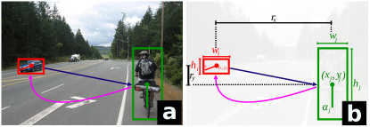
Figure 5: Attributed pairwise relations defined from object hypotheses predictions. $w_{i}$: bounding box width, $h_{i}$: bounding box height, $(x_{i},y_{i})$: coordinates of the center of the bounding box, and $\alpha_{i}$: object viewpoint.

4.3 Multiclass Classification for coupled object
viewpoint estimation

In order to enforce consistency between the local response $\psi^{l}$, given by the detector, and the contextual response $\psi^{c}$, given by the context-based viewpoint classifier, we define object viewpoint classification as a classification problem (Eq. 8) based on the coupled-response $\Psi=(\psi^{l},\psi^{c})$. In this paper we evaluate the performance of two methods for this particular task.

The first method, Probabilistic Combination, is inspired by [49]. As Eq. 9 presents, to classify the viewpoint $\hat{\alpha_{i}}$ of an object $o_{i}$ we perform MAP inference for the coupled-response $\Psi_{i}$ over the discrete viewpoint classes $\alpha_{k}$.

$$\hat{\alpha_{i}} =\arg\max_{\alpha_{k}}(~{}p(\overline{\alpha}_{k}^{+}|\Psi_{i})~{})$$ (9)

$$=\arg\max_{\alpha_{k}}(~{}p(\Psi_{i}|\overline{\alpha}_{k}^{+})p(\overline{\alpha}_{k}^{+})~{})$$

In this equation, the term $p(\Psi_{i}|\overline{\alpha}_{k}^{+})$ is estimated using KDE from the coupled-responses $\Psi=[\psi^{l},\psi^{c}]$ of object hypotheses collected from a validation set. The term $p(\overline{\alpha}_{k}^{+})$ is determined by the proportion of objects with viewpoint $\alpha_{k}$ in the validation set.

The second method, Linear Combination, is based on linear Support Vector Machines (SVM). Specifically we use the method from Crammer and Singer [10] for the implementation of multiclass SVMs. Following this procedure, the object viewpoint classification problem is defined as:

$$\hat{\alpha_{i}}=\arg\max_{\alpha_{k}}(W_{k}\cdot\Psi_{i}).$$ (10)

Here the problem is to learn the matrix of weights $W_{k}$ of the SVM Model that will be used to predict the class, in this case the object viewpoints $\alpha_{k}$. Similar to the previous classifier, here we collect the response vectors $\Psi_{i}$ from validation images. In addition, we perform 3-fold cross validation to estimate the cost parameter used for training the SVM classifier.

4.4 Kernel Density Estimation

Kernel Density Estimation (KDE) is performed using the odKDE variant proposed in [28]. Under odKDE the sample distribution is modeled by a $C$-component mixture of Gaussians as $f(x)=\sum_{i=1}^{C}{\omega_{i}\cdot\phi_{\Sigma_{si}}(\ x-\mu_{i})}$, where $\phi_{\Sigma_{si}}$ is a Gaussian centered in $\mu_{i}$ and with covariance matrix $\Sigma_{si}$. The effect of each component is measured by the mixture weights $\omega_{i}$ with $\sum{\omega_{i}}=1$. As Eq.11 shows, the KDE $p(x)$ of the distribution is determined by the convolution of the sample distribution $f(x)$ with a Gaussian kernel $\phi_{H}(x)$.

$$p(x) =\phi_{H}(x)*f(x)$$ (11)

$$=\sum_{i=1}^{C}{\omega_{i}\cdot\phi_{\Sigma_{i}}(\ x-\mu_{i})}$$

where $\Sigma_{i}=H_{i}+\Sigma_{si}$, and $H_{i}$ is the bandwidth of the convolution kernel. For more details related to the computation of $H_{i}$ please refer to [28]. In our experiments, the samples $x$ take the form of the attributes of the pairwise relations $r_{ij}$ between objects (Eq. 5), the detection scores $s_{i}$ (Eq. 6) or the coupled-response $\Psi_{i}$ (Eq. 9). In these equations, KDE is used to estimate the value of their respective conditional terms.

KITTI dataset [16]
	MPPE		AVP
Method	Oracle	Lopez et al. [32]	Oracle	Lopez et al. [32]
Aggressive-RF1	0.37	0.27	0.74	0.06
Aggressive-RF2	0.22	0.17	0.60	0.06
Cautious-RF1	0.41	0.30	0.72	0.06
Cautious-RF2	0.36	0.27	0.66	0.07
Method	Oracle	Geiger et al. [17]	Oracle	Geiger et al. [17]
Aggressive-RF1	0.39	0.28	0.68	0.10
Aggressive-RF2	0.23	0.20	0.55	0.14
Cautious-RF1	0.40	0.32	0.69	0.09
Cautious-RF2	0.36	0.31	0.64	0.10
Method	Oracle	Ren et al. [52]	Oracle	Ren et al. [52]
Aggressive-RF1	0.48	0.36	0.78	0.28
Aggressive-RF2	0.28	0.29	0.60	0.25
Cautious-RF1	0.43	0.44	0.74	0.30
Cautious-RF2	0.39	0.40	0.67	0.28

Table 2: Contextual object viewpoint classification mean precision for pose estimation (MPPE) and Average viewpoint precision (AVP) for the proposed methods on the KITTI [16] dataset. We report results on hypotheses collected with DPM-based methods ([32, 17]) and a CNN-based method (Faster RCNN [29] + viewpoint CNN [52]). Note how the methods that perform cautious relational inference tend to have superior performance than their aggressive counterparts.

5 Evaluation

5.1 Experimental Details

Datasets: We focus on urban scenes. For this reason, we conduct experiments on the object detection set of the KITTI benchmark [16]. The KITTI dataset is collected from a car-mounted camera, resembling an autonomous navigation setting. We consider “car” as category of interest as it occurs multiple times in each image of this dataset. This dataset presents a variety of difficult scenarios ranging from object instances with high occlusions to object instances with very small size. Furthermore, it provides precise annotations from objects in the 2D image and in the 3D space, including their respective viewpoints. Since this is a benchmark dataset, annotations are not available for the test set. For this reason, we focus our experiments on the training set. Each image of the training set belongs to a video sequence; we use the sequence ID and the time stamp of each image in order to sort them by video sequence. Then, the training images belonging to each sequence are split in three disjoint subsets in chronological order. The first subset is used for learning the relations between object instances (see Section 3.2). The second subset is used to learn the combination of local and contextual information (see Section 3.4). The third set is used to evaluate the performance of the proposed method.

Since the focus of this work is on reasoning about relations between objects, we focus our evaluation on the subset of 5266 images with two or more object instances.

Methods: In our experiments, we define four methods to perform context-based classification based on the combination of the following parameters. As presented in Section 3.2 our methods are defined as Aggressive or Cautious depending on the type of relational inference they perform. In addition, we define pairwise relations following two formats. The first format, $RF1$, is as defined in Section 4.2. The second format, $RF2$, is similar to $RF1$ but removing the viewpoint attribute $\alpha_{j}$, thus producing a relation $r_{ij}=(rx_{ij},ry_{ij},rs_{ij})$ with four attributes that encodes only relative location and scale.

5.2 Contextual Object Viewpoint Classification

The objective of this first experiment is to evaluate the performance of the algorithm at estimating the viewpoint of the object hypotheses purely based on its neighboring objects (see Section 3.2).

We evaluate our methods following two settings to collect object hypotheses. The first setting starts from an “Oracle” detector, thus producing perfectly localized hypotheses. Furthermore, in this oracle setting, while the viewpoint of an object is being classified, the ground truth viewpoints of its neighbor objects are used. This setting will show whether there is something to gain from reasoning about object relations for object viewpoint classification.

The second setting uses the previously mentioned viewpoint-aware detectors ([17, 32, 52, 63]) to collect object hypotheses. Then, the viewpoint of each object is estimated based on its neighbors taking into account the detection scores and predicted viewpoints. This last setting represents a more realistic scenario.

In this experiment we will use the Mean Precision for Pose Estimation (MPPE) and Average Viewpoint Precision (AVP) as performance metrics. The MPPE metric is traditionally used to measure viewpoint classification [31, 32, 48, 53]. MPPE is computed as the average of the diagonal of the class-normalized confusion matrix of the viewpoint classifier. Additionally, taking into account the observations made by [51], we include AVP [63] as an additional performance metric. AVP a is metric derived from Average Precision (AP), traditionally used to measure object localization performance, extended to measure the capability of a viewpoint-aware detector at predicting the location and viewpoint of object instances, jointly. We report the results of this experiment in Table 2.

Discussion: Notice first that when inspecting the MPPE performance obtained using an Oracle detector all the performance values are above chance levels ($\sim$0.13 for classification of 8 discrete viewpoints). This suggests that indeed there is some information about the viewpoint of the unknown object that can be gathered from its neighboring objects - hence it makes sense to reason about object relations for object viewpoint estimation. We see a similar trend for the methods that collect object hypotheses using one of the viewpoint-aware detectors ([17, 32, 52, 63]), but with a drop in performance. This is to be expected, since some of the object hypotheses used as sources of context are false positives which introduce noise in the inference. We can also see that the performance increases as we go to the CNN-based method. Given the fact that between the Oracle-based methods the only difference is the learned relational model used to compute the pairwise term $v(o_{i},o_{j})$ (Section 3.1.1 and 3.2) and that this model depends on the annotations and hypotheses being collected by the detector, it is evident that using a better performing detector can help improving the modeling of context and hence improves viewpoint classification.

We can notice that the values of MPPE are significantly lower when compared to their respective AVP counterparts. This is to be expected since AVP is a harder metric which also measures the level to which an object hypothesis is properly localized. Furthermore, we notice that AVP values for the CNN-based methods are superior again to those of the DPM-based methods. This confirms the known fact that DPM-based methods, while being able to perform viewpoint classification to some extent, have a limited capability at properly localizing object instances as compared to the CNN-based methods.

Regarding relational inference type, we notice that in all cases cautious relational inference has superior performance than aggressive inference. In the oracle setting, methods based on cautious inference outperform their aggressive counterparts by 7 percentage points (pp). In the realistic setting, this difference increases to 8 pp. This is probably caused by the extra room for improvement that is produced by noise in standard detectors.

Finally, related to the format used to represent the pairwise relations, it seems that relations defined by RF1 (i.e. including the pose of the contextual objects) have superior performance over RF2. In purely contextual classification, relations defined by RF1 outperform those defined by RF2 by 11 and 12 pp, in the ideal and realistic setting, respectively. For the case of joint localization and viewpoint prediction, on the one hand, we notice that the performance of Oracle baselines are led by methods based on RF1-type relations with an average difference of 16 AVP points. Keeping in mind that RF1 relations are similar to RF2 relations with the difference that RF1 includes the viewpoints of the contextual instances, this suggests that considering viewpoint information from other object instances is an informative contextual cue for the problem at hand. On the other hand, we notice that when starting from the hypotheses collected with the viewpoint-aware detectors, the difference between RF1 and RF2 is not so outspoken. In fact, for the case of the DPM-based methods, which have noisier viewpoint predictions, this difference is almost nonexistent or reverted. For the case of the CNN-based method, RF1-type relations still outperform their RF2 counterparts with 3 AVP points on average. Finally, compared to the DPM-based methods, the difference in performance between the Oracle and the real detectors is more reduced for the CNN-based methods.

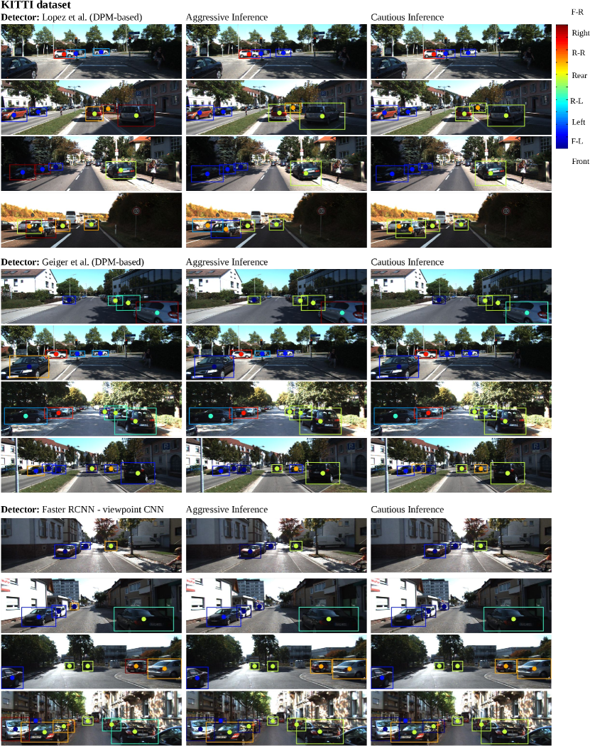
Figure 6: Context-based viewpoint classification qualitative results for cars in the KITTI [16]. Object viewpoint classification results are encoded in jet scale (see color bar). Continuous line, predicted object viewpoint; Circle, ground-truth object viewpoint (Best viewed in color).

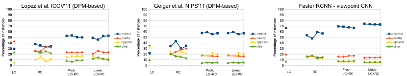
Figure 7: Viewpoint classification error. For each of the baselines we show the percentage of object instances whose viewpoint is: predicted correctly (blue), confused with a nearby viewpoint class (red), confused with an opposite viewpoint (yellow), and confused with other viewpoints (green). We report results for both the local methods (LC) which only consider local information, the relational methods (RC) which only consider contextual information and the probabilistic and linear combination of both cases. For the methods based on contextual information we report results for four variants Aggressive-RF1, Aggressive-RF2, Cautious-RF1 and Cautious-RF2. It is noticeable that the proposed context-based methods assist local methods by addressing nearby and other type errors.

5.3 Combining Local and Contextual cues for Viewpoint Estimation

In this experiment we measure the performance of the combination of local and contextual information for object viewpoint estimation. Specifically, we evaluate the late fusion of the responses from the local classifier (LC), i.e. the viewpoint-aware detector, and the relational classifier (RC), i.e. the viewpoint classifier based on the context (see Sections 3.4 & 4.3). The objective of this experiment is to verify whether enriching the local classifier with contextual information can increase the performance initially obtained by the local classifier alone. For this experiment we use the same MPPE and AVP performance metrics as in the previous experiment. We report quantitative results of this experiment in Tables 3 and 4. See Figure 6 for some qualitative results.

KITTI dataset [16] - MPPE performance
	None	Aggressive		Cautious
		RF1	RF2	RF1	RF2
None	-	0.27	0.17	0.30	0.27
Lopez et al.[32]	0.32	0.37	0.41	0.34	0.37	Prob.
		0.28	0.35	0.41	0.44	Linear
None	-	0.28	0.20	0.32	0.31
Geiger et al.[17]	0.44	0.39	0.45	0.40	0.41	Prob.
		0.39	0.45	0.36	0.39	Linear
None	-	0.36	0.29	0.44	0.40
Ren et al.[52]	0.61	0.56	0.53	0.51	0.50	Prob.
		0.59	0.59	0.59	0.58	Linear

Table 3: Combined object viewpoint classification performance on KITTI [16]. Mean Precision on Pose Estimation (MPPE) performance is presented for the combination of the local classifier (LC) and relational classifier (RC) using the methods based on probabilistic and linear combination, respectively. We report results on hypotheses collected with DPM-based methods ([32, 17]) and CNN-based methods (Faster RCNN [29] + viewpoint CNN [52]).

KITTI dataset [16] - AVP performance
	None	Aggressive		Cautious
		RF1	RF2	RF1	RF2
None	-	0.06	0.06	0.06	0.07
Lopez et al.[32]	0.06	0.07	0.08	0.08	0.08	Prob.
		0.08	0.08	0.09	0.11	Linear
None	-	0.10	0.14	0.09	0.10
Geiger et al.[17]	0.07	0.17	0.17	0.17	0.18	Prob.
		0.18	0.20	0.19	0.19	Linear
None	-	0.28	0.25	0.30	0.28
Ren et al.[52]	0.37	0.36	0.37	0.36	0.37	Prob.
		0.39	0.39	0.39	0.39	Linear

Table 4: Combined object viewpoint classification performance on KITTI [16]. Average Viewpoint Precision (AVP) performance is presented for the combination of the local classifier (LC) and relational classifier (RC) using the methods based on probabilistic and linear combination, respectively. We report results on hypotheses collected with DPM-based methods ([32, 17]) and CNN-based methods (Faster RCNN [29] + viewpoint CNN [52]).

Discussion: At first glance, when focusing on the MPPE metric, we can notice that the dominance of methods based on cautious inference over those based on aggressive inference is not as marked as it was on the purely-contextual experiment. For the case of the combination of local and contextual responses using the method based on linear combination (SVM-based), the performance difference between methods using these two types of inference is reduced to 6 MPPE points. For the case when the probabilistic (KDE-based) method is used for combining LC and RC, methods based on aggressive inference outperform methods that perform cautious inference by 3 MPPE points. We can verify in Table 3 that the combination of some context-based methods with the local classifiers manages to improve the initial performance obtained by the local classifier, especially for the case of the DPM-based methods ([17, 32]). For the case of joint object localization and viewpoint estimation (AVP metric), we can notice that superior performance is achieved when using the linear method for late fusion. Moreover, similar as with the MPPE metric, the improvement brought by the contextual model is higher over the DPM-based methods ($\sim$10 AVP points) than over the CNN-based methods (2 AVP points). This shows that the proposed context-based method is not only able to provide improvements in terms of viewpoint but also in terms of object localization.

In Figure 6 we can notice that by considering contextual information (2nd and 3rd columns) we are able to correct some of mistakes initially made by the local detector (1st column).

KITTI dataset [16]
Local Information
	Lopez et al. [32]			Geiger et al. [17]			Ren et al. [52]
	Low	High	All	Low	High	All	Low	High	All
	0.07	0.05	0.06	0.07	0.07	0.07	0.39	0.36	0.37
Contextual Information
	Lopez et al. [32]			Geiger et al. [17]			Ren et al. [52]
Method	Low	High	All	Low	High	All	Low	High	All
Aggressive-RF1	0.05	0.07	0.06	0.08	0.12	0.10	0.26	0.30	0.28
Aggressive-RF2	0.04	0.08	0.06	0.10	0.16	0.14	0.22	0.28	0.25
Cautious-RF1	0.05	0.07	0.06	0.06	0.10	0.09	0.30	0.31	0.30
Cautious-RF2	0.05	0.08	0.07	0.08	0.12	0.10	0.27	0.29	0.28
Local + Contextual Information (Probabilistic Combination)
	Lopez et al. [32]			Geiger et al. [17]			Ren et al. [52]
Method	Low	High	All	Low	High	All	Low	High	All
Aggressive-RF1	0.06	0.08	0.07	0.14	0.19	0.17	0.36	0.36	0.36
Aggressive-RF2	0.07	0.09	0.08	0.15	0.19	0.17	0.38	0.37	0.37
Cautious-RF1	0.07	0.09	0.08	0.14	0.20	0.17	0.36	0.35	0.36
Cautious-RF2	0.06	0.10	0.08	0.15	0.20	0.18	0.38	0.36	0.37
Local + Contextual Information (Linear Combination)
	Lopez et al. [32]			Geiger et al. [17]			Ren et al. [52]
Method	Low	High	All	Low	High	All	Low	High	All
Aggressive-RF1	0.06	0.09	0.08	0.15	0.21	0.18	0.40	0.39	0.39
Aggressive-RF2	0.06	0.09	0.08	0.17	0.22	0.20	0.40	0.39	0.39
Cautious-RF1	0.08	0.11	0.09	0.16	0.22	0.19	0.40	0.39	0.39
Cautious-RF2	0.10	0.12	0.11	0.16	0.22	0.19	0.40	0.39	0.39

Table 5: Average viewpoint precision (AVP) for the proposed method for context-based viewpoint classification on KITTI [16] dataset. We report results on hypotheses collected with DPM-based methods ([32, 17]) and CNN-based methods (Faster RCNN [29] + viewpoint CNN [52]). Note how the methods focused on local information tend to dominate on images with a low number of instances (Low subset), while the context-based methods have superior performance on images with a high number of instances (High subset).

5.4 Deeper Analysis

In order to identify the scenarios in which the proposed contextual approach benefits methods based on local information, we provide an analysis on common viewpoint classification errors (Section 5.4.1) and on the effect that the number of occurring object instances has in object viewpoint classification performance (Section 5.4.2).

5.4.1 Viewpoint Classification Error Analysis

We provide now an analysis on common viewpoint classification errors made by both the local and the proposed context-based method. Following the protocol from [51] these errors are grouped as ”opposite” (viewpoints with a difference of 180 degrees), ”nearby” (viewpoints from neighboring viewpoint classes) and ”other” (all the other viewpoints). In Figure 7 we show the percentage of instances that belong to each of these three groups plus the percentage of object instances that were predicted correctly. Following the previous experiments, we show the performance when the local classifier (LC), the relational classifier (RC) and the combination of both is employed.

Discussion: At first glance, Figure 7 further confirms the observations made in previous experiments. When focusing on the local classifier we can notice that the CNN-based method has a higher number of correct predictions (blue) when compared to the DPM-based methods. It is also noticeable that the most common type of viewpoint estimation error lies in the nearby group (orange) for all the local methods.

When focusing on the purely context-based methods (RC), we can notice that for all cases the nearby error is reduced. Moreover, we can notice that for the case of the DPM-based methods, there is some increase in the percentage of object instances classified correctly.

Finally, when both local and contextual information is considered, the number of correctly predicted instances is further increased for all the local methods, especially when using a linear combination method. For the DPM-based methods the nearby errors are further reduced w.r.t. to results obtained in the purely contextual case. Moreover, we notice that for all the cases, other-type errors get attenuated. We can notice that for the case of CNN-based methods, the combination of local and contextual information produces a reduction of the nearby-type errors while keeping the opposite and other errors at the level of the local method.

The previous observations in combination with Figure 7 provide insight on the benefits that the proposed contextual method brings to the methods based on local information. First, for the case of DPM-based methods ([17, 32]), the context-based methods bring improvement in performance by reducing errors of type nearby and other. Moreover, for the case of [17], the proposed context-based method is able to also address errors between opposite viewpoints. Finally, for the case of the CNN-based method, contextual information complements methods based on local information by reducing errors between nearby viewpoints.

5.4.2 Effect of the Number of Objects per Image

The proposed method fully relies on the exploitation of relations between objects (Section 3.1). Since these relations are directly defined from object instances occurring (or detected) in images, in this experiment we measure the effect that the number of object instances has on the effectiveness of context-based methods. Towards this goal, in this experiment we measure performance in two independent subsets of images. In order to define these subsets, we first compute the average number of annotated object instances per image in the dataset. In the case of the KITTI dataset this average value is 5 objects per image. The Low subset, is composed by images with a number of annotated object instances less or equal to the average, while the High subset is composed by the images with higher number of objects. We report the AVP performance of these two subsets and the subset composed by All the images in Table 5.

Discussion: We can notice that when only considering local information, higher performance is achieved when focusing on images with few object instances, which likely implies lower inter-object occlusion and a lower number of instances with small size. On the contrary, when only considering contextual information, higher performance is achieved always for the High subset. This suggests that while the local classifier is able to handle effectively images with few objects (possibly with large size and low level of occlusions), the contextual information is able to compensate for some of the hard scenarios (low object size and occluded objects) of the local classifier. Finally, for the case when local and contextual information is combined, we can notice that for the DPM-based local methods, the performance on the High subset is still superior to that on the Low subset. For the CNN-based local method we notice that the performance in both Low and High subsets tend to be comparable. This is to be expected since the DPM-based methods are less effective than the CNN-based methods, hence leaving more room for improvement for the contextual model. For the linear combination with the CNN-based method, we notice that the contextual model is able to push performance of the local classifier on the High subset for $\sim$3 AVP points while only 1 AVP point of the case of the Low subset. This shows that the proposed method has the potential of improving both object localization and viewpoint estimation performance especially for the case of crowded scenarios, i.e. images with high number of instances, where inter-object occlusions and instances with small size are likely to occur.

6 Limitations and Future Work

We have presented a method to perform object viewpoint estimation by using contextual information derived from the other object instances occurring in the scene. Our empirical results show that there is a clear potential for this type of contextual cue on improving object viewpoint classification. Moreover, we have shown that considering contextual information reduces prediction errors of type nearby and other (Section 5.4.1). However, in its current state, the proposed method has some limitations that could be addressed in further work. These limitations are closely related to the two main assumptions behind our method. First, our model assumes there is a structured behavior (occurrence, viewpoint, localization, etc.) between entities (objects) in the scene. Second, during test time it is required for the local detector to have an acceptable level of performance in order to feed our contextual model with informative cues and to be able to be improved from.

Regarding the first assumption, in our experiments, the KITTI dataset resembles a Urban setting and due its large volume of data, multiple plausible scene states (object occurrence, location, size, viewpoints, etc.) are presented. Moreover, this is done for different scene types, i.e. highway, urban, residential, etc. Hence, the KITTI dataset constitutes a representative dataset for the setting to be modeled. On the contrary, for the case of a more biased dataset (either at object locations, viewpoints, etc.), there might not be sufficient representative information to accurately model the relational behavior of the objects in the scene. This is in line with the findings from the Collective Classification and Link-based Classification communities [5, 25, 41, 54]. Those findings state that methods that reason about links, or relations, between entities have an improved performance when operating on a setting with high link density. It is important to notice that link density does not only refer to the quantity (amount) of the links between entities, but also refers to the quality (representativeness) of such links. In our particular setting, link density is directly influenced by the objects occurring in the images, more specifically, the relations between them, i.e. the relative locations and viewpoints in which these objects co-occur. In this regard, the KITTI dataset has a high amount of links while being diverse and covering different scenarios of co-occurring object viewpoints. Based on this, a reasonable hypothesis is that the proposed context-based method may underperform when learning object relations from biased datasets showing poor link density.

Regarding the second assumption, when using a low-performing local detector, while allowing significant room for improvement, it will introduce noise to the contextual model and further complicate the following processes. On the contrary, having a highly-performing detector will significantly reduce the cases in which the context model could produce improvement. In our experiments we have noted that by going from DPM-based viewpoint-aware detectors to CNN-based methods we can increase the overall performance while still being able to bring improvement via the proposed context-based method. This assumption is related to the ratio between true and false positives predicted by the local classifier. This ratio is important if we consider that the number of relations has a quadratic growth w.r.t. the number of object hypotheses, hence introducing a significant amount of noise in the context-based classification process. This ratio is known as class skewness, or labeled proportion, in the collective classification literature [7, 38, 40, 59], more specifically when focusing on within network classification tasks where predictions about some nodes are based on other nodes. In this type of tasks, class skewness measures the proportion of data that is known, or predicted with certainty, w.r.t. the whole data. In scenarios where class skewness is low, there is not enough certain information to guide the inference process. In scenarios with high class skewness, the performance of collective classification is better or comparable to that of local classification.

An additional weak point of the proposed method lies in the way in which it combines the responses from the local and relational classifiers. A more structured approach to improve the combination of these responses is by formulating the object viewpoint classification problem within a Conditional Random Field (CRF) setting. This structured setting could be defined over an undirected graph $G=(V,E)$ where the nodes $V$ are the objects and edges $E$ are the relations between objects (as defined in Section 4.2). In this case the states that a node (object) may take are defined by the possible viewpoint values $\alpha$. The Unary potential is defined by the local evidence given by the object detector – more specifically, the confidence of the classifier over different object viewpoints. The Pairwise potential of the edges is defined by the distribution of a relation $r_{ij}$ occurring between objects $o_{i}$ and $o_{j}$ over different viewpoint values. This potential is estimated in a similar fashion as the pairwise term $v(o_{i},o_{j})$ from Equation 5. Having these potentials in place, we could solve the CRF in order to find the global optimal configuration that satisfies both the local response given by the object detector as well as the object relations considered by our model.
On the positive side, following this setting there are several factors that can be evaluated, e.g. graph topology, regularization, edge representation, that can be optimized in order to push performance further. However, on the weak side, the proposed CRF-method has the disadvantage of being more computationally expensive when compared to the proposed method.

Not withstanding these limitations and regardless of the collective classification method that is used, we have shown that performing collective inference results in performance gains on object viewpoint estimation. This finding becomes even more relevant when we keep in mind the fact that the proposed context-based method has proven to have complementarity w.r.t. local methods, and that all this has been achieved while starting from one of the simplest collective classification methods. This suggests that reasoning about object relations in 2D image space can indeed assist the task of object viewpoint classification, and that there is a clear potential for more advanced methods for collective classification to further improve object viewpoint estimation performance.

7 Conclusions

In this paper we have presented a method to exploit contextual information, in the form of relations between objects, for object viewpoint classification in the 2D image space. Our experiments show that even when contextual information alone cannot solve the viewpoint estimation problem accurately, it is able to provide good priors about the location and viewpoint of objects. This characteristic can be useful for tasks such as object proposal generation driven by object relations. In addition, our experiments show that in the absence of local appearance information about the object to be classified, performing cautious inference about object relations outperforms its aggressive counterpart. Our analysis reveals that the proposed context-based method complements methods that only consider local information in two ways: First, it is able to reduce viewpoint errors related to nearby and other non-opposite types. Second, it produces superior performance in settings where a high number of object instances occur. Investigating more structured methods to enforce global consistency and to model object relations between multiple object categories constitutes our next steps for future work.

Acknowledgments: This work was supported by the FWO project SfS, the KU Leuven PDM Grant PDM/16/131, and a NVIDIA Academic Hardware Grant.

References

- [1] B. Alexe, N. Heess, Y. W. Teh, V. Ferrari, Searching for objects driven by context, in: NIPS, 2012.
- [2] L. Antanas, M. V. Otterlo, J. Oramas M, T. Tuytelaars, L. D. Raedt, There are plenty of places like home: Using relational representations in hierarchies for distance-based image understanding, Neurocomputing 123 (2014) 75–85.
- [3] S. Y. Bao, M. Bagra, Y. Chao, S. Savarese, Semantic structure from motion with points, regions, and objects, in: CVPR, 2012.
- [4] S. Y. Bao, S. Savarese, Semantic structure from motion, in: CVPR, 2011.
- [5] M. Bilgic, G. Namata, L. Getoor, Combining collective classification and link prediction, in: ICDM Workshops, 2007.
- [6] S. B. C. Galleguillos, B. McFee, G. Lanckriet, Multi-class object localization by combining local contextual interactions., in: CVPR, 2010.
- [7] S. Chakrabarti, B. Dom, P. Indyk, Enhanced hypertext categorization using hyperlinks, in: SIGMOD, 1998.
- [8] M. J. Choi, J. J. Lim, A. Torralba, A. S. Willsky, Exploiting hierarchical context on a large database of object categories, in: CVPR, 2010.
- [9] R. G. Cinbis, S. Sclaroff, Contextual object detection using set-based classification, in: ECCV, 2012.
- [10] K. Crammer, Y. Singer, On the algorithmic implementation of multiclass svms, JMLR 2 (2001) 265–292.
- [11] C. Desai, D. Ramanan, C. Fowlkes, Discriminative models for multi-class object layout, IJCV 95 (1) (2011) 1–12.
- [12] M. Everingham, L. Van Gool, C. K. I. Williams, J. Winn, A. Zisserman, The PASCAL Visual Object Classes Challenge 2012 (VOC2012) Results.
- [13] P. F. Felzenszwalb, R. B. Girshick, D. McAllester, D. Ramanan, Object Detection with Discriminatively Trained Part-Based Models, TPAMI 32 (9) (2010) 1627–1645.
- [14] S. Fidler, J. Yao, R. Urtasun, Describing the scene as a whole: Joint object detection, scene classification and semantic segmentation, in: CVPR, 2012.
- [15] D. A. Forsyth, J. Malik, M. M. Fleck, H. Greenspan, T. Leung, S. Belongie, C. Carson, C. Bregler, Finding pictures of objects in large collections of images, in: ECCV, 1996.
- [16] A. Geiger, P. Lenz, R. Urtasun, Are we ready for autonomous driving? the kitti vision benchmark suite, in: CVPR, 2012.
- [17] A. Geiger, C. Wojek, R. Urtasun, Joint 3d estimation of objects and scene layout, in: NIPS, 2011.
- [18] A. Ghodrati, M. Pedersoli, T. Tuytelaars, Is 2d information enough for viewpoint estimation?, in: BMVC, 2014.
- [19] D. Glasner, M. Galun, S. Alpert, R. Basri, G. Shakhnarovich, Viewpoint-aware object detection and pose estimation, in: CVPR, 2011.
- [20] G. Heitz, D. Koller, Learning spatial context: Using stuff to find things, in: ECCV, 2008.
- [21] D. Hoiem, A. Efros, M. Hebert, Closing the loop in scene interpretation, in: CVPR, 2008.
- [22] D. Hoiem, C. Rother, J. M. Winn, 3d layoutcrf for multi-view object class recognition and segmentation, in: CVPR, 2007.
- [23] L. G. Hulbert, M. L. Corrêa da Silva, G. Adegboyega, Cooperation in social dilemmas and allocentrism: a social values approach, European Journal of Social Psychology 31 (6) (2002) 641–657.
- [24] A. Jain, A. Gupta, L. S. Davis, Learning what and how of contextual models for scene labeling, in: ECCV, 2010.
- [25] D. Jensen, J. Neville, Autocorrelation and linkage cause bias in evaluation of relational learners, in: Inductive Logic Programming, vol. 2583, Springer Berlin Heidelberg, 2003, pp. 101–116.
- [26] R. Juránek, A. Herout, M. Dubská, P. Zemcík, Real-time pose estimation piggybacked on object detection, in: ICCV, 2015.
- [27] B. Kim, M. Sun, P. Kohli, S. Savarese, Relating things and stuff by high-order potential modeling, in: ECCV Workshops, 2012.
- [28] M. Kristan, A. Leonardis, Online discriminative kernel density estimator with gaussian kernels, TSMC 44 (3) (2013) 355–365.
- [29] A. Krizhevsky, I. Sutskever, G. E. Hinton, Imagenet classification with deep convolutional neural networks, in: NIPS, 2012.
- [30] C. Li, A. Kowdle, A. Saxena, T. Chen, Toward holistic scene understanding: Feedback enabled cascaded classification models, TPAMI 34 (7) (2012) 1394–1408.
- [31] J. Liebelt, C. Schmid, Multi-view object class detection with a 3d geometric model, in: CVPR, 2010.
- [32] R. Lopez, T. Tuytelaars, Deformable part models revisited: A performance evaluation for object category pose estimation., in: CVPR Workshops., 2011.
- [33] S. A. Macskassy, Leveraging contextual information to explore posting and linking behaviors of bloggers, in: ASONAM, 2010.
- [34] S. A. Macskassy, On the study of social interactions in twitter, in: ICWSM, 2012.
- [35] S. A. Macskassy, M. Michelson, Why do people retweet? anti-homophily wins the day!, in: ICWSM, 2011.
- [36] S. A. Macskassy, F. Provost, A simple relational classifier, in: KDD Workshops, 2003.
- [37] S. A. Macskassy, F. Provost, S. A. Macskassy, Suspicion scoring of networked entities based on guilt-by-association, collective inference, and focused data access 1, in: NAACSOS, 2005.
- [38] S. A. Macskassy, F. J. Provost, Classification in networked data: A toolkit and a univariate case study, JMLR 8 (2007) 935–983.
- [39] L. McDowell, K. M. Gupta, D. W. Aha, Cautious inference in collective classification, in: AAAI, 2007.
- [40] L. McDowell, K. M. Gupta, D. W. Aha, Cautious collective classification, JMLR 10 (2009) 2777–2836.
- [41] J. Neville, D. Jensen, Leveraging relational autocorrelation with latent group models, in: ICDM, 2005.
- [42] J. Neville, D. D. Jensen, Iterative classification in relational data, in: Workshop on SRL at AAAI, 2000.
- [43] J. Oramas M, L. De Raedt, T. Tuytelaars, Allocentric pose estimation, in: ICCV, 2013.
- [44] J. Oramas M, L. De Raedt, T. Tuytelaars, Towards cautious collective inference for object verification, in: WACV, 2014.
- [45] J. Oramas M, T. Tuytelaars, Recovering hard-to-find object instances by sampling context-based object proposals, Computer Vision and Image Understanding 152 (2016) 118 – 130.
- [46] M. B. P. Sen, G. Namata, L. Getoor, Collective classification, in: Encyclopedia of Machine Learning, 2010, pp. 189–193.
- [47] B. Pepik, M. S., P. G., B. Schiele, Teaching 3d geometry to deformable part models, in: CVPR, 2012.
- [48] B. Pepik, M. Stark, P. Gehler, B. Schiele, Teaching 3d geometry to deformable part models, in: CVPR, 2012.
- [49] R. Perko, A. Leonardis, A framework for visual-context-aware object detection in still images, in: CVIU, vol. 114, 2010, pp. 700–711.
- [50] M. H. Quinn, A. D. Rhodes, M. Mitchell, Active object localization in visual situations, CoRR abs/1607.00548.
- [51] C. Redondo-Cabrera, R. J. López-Sastre, Y. Xiang, T. Tuytelaars, S. Savarese, Pose estimation errors, the ultimate diagnosis, in: ECCV, 2016.
- [52] S. Ren, K. He, R. Girshick, J. Sun, Faster R-CNN: Towards real-time object detection with region proposal networks, in: NIPS, 2015.
- [53] S. Savarese, L. Fei-Fei, 3d generic object categorization, localization and pose estimation, in: ICCV, 2007.
- [54] P. Sen, G. Namata, M. Bilgic, L. Getoor, B. Gallagher, T. Eliassi-Rad, Collective classification in network data, AI Magazine 29 (3) (2008) 93–106.
- [55] J. M. Shubham Tulsiani, Viewpoints and keypoints, in: CVPR, 2015.
- [56] Z. Song, Q. Chen, Z. Huang, Y. Hua, S. Yan, Contextualizing object detection and classification, in: CVPR, 2011.
- [57] H. Su, C. R. Qi, Y. Li, L. J. Guibas, Render for cnn: Viewpoint estimation in images using cnns trained with rendered 3d model views, in: ICCV, 2015.
- [58] M. Sun, S. Y. Bao, S. Savarese, Object detection using geometrical context feedback, IJCV 100 (2) (2012) 154–169.
- [59] B. Taskar, P. Abbeel, D. Koller, Discriminative probabilistic models for relational data, in: UAI, 2002.
- [60] A. A. E. Tomasz Malisiewicz, Beyond categories: The visual memex model for reasoning about object relationships, in: NIPS, 2009.
- [61] H. C. Triandis, E. M. Suh, Cultural influences on personality., Annual Review of Psychology 53 (2002) 133–160.
- [62] X. Wang, G. Sukthankar, Multi-label relational neighbor classification using social context features, in: KDD, 2013.
- [63] Y. Xiang, R. Mottaghi, S. Savarese, Beyond pascal: A benchmark for 3d object detection in the wild, in: WACV, 2014.
- [64] Y. Xiang, S. Savarese, Object detection by 3d aspectlets and occlusion reasoning, in: ICCV Workshops, 2013.
- [65] J. S. Yedidia, Message-passing algorithms for inference and optimization, Journal of Statistical Physics 145 (4) (2011) 860–890.
- [66] Z. Zia, M. Stark, K. Schindler, Are cars just 3d boxes? - jointly estimating the 3d shape of multiple objects, in: CVPR, 2014.