The classification of linked $3$-manifolds in $6$-space.

Abstract.

Let $M_{1}$ and $M_{2}$ be closed connected orientable $3$-manifolds. We classify the sets of smooth and piecewise linear isotopy classes of embeddings $M_{1}\sqcup M_{2}\rightarrow S^{6}$.

1. Introduction.

1.1. Statement of the result.

All maps and manifolds in the text are smooth unless specifically stated otherwise.

For a manifold $N$ denote by $E^{m}(N)$ the set of isotopy classes of embeddings $N\rightarrow S^{m}$. The main result of the paper is Theorem 1.11 giving a classification of $E^{6}(M_{1}\sqcup M_{2})$ for arbitrary closed connected orientable $3$-manifolds $M_{1}$ and $M_{2}$. As a corollary we also get a piecewise linear (PL) classification, see Theorem 1.18 in §1.2.

We start with the previously known classifications of $E^{6}(S^{3}\sqcup S^{3})$ and $E^{6}(N)$, where $N$ is a closed connected orientable $3$-manifold. These results are later used in our proofs. In §1.3 we also give a brief general survey on embeddings classification.

An embedding $g:S^{3}\rightarrow S^{6}$ is called trivial if it is isotopic to the standard embedding. The isotopy class of a trivial embedding is also called trivial. The embedded connected sum operation $\#$ (see §1.4) defines a group structure on $E^{6}(S^{3})$. Operation $\#$ also defines an action of $E^{6}(S^{3})$ on $E^{6}(N)$ for any closed connected orientable $3$-manifold $N$.

Theorem 1.1 (A. Haefliger).

$E^{6}(S^{3})\cong{\mathbb{Z}}$.

Let

$$r:E^{6}(S^{3})\rightarrow{\mathbb{Z}}$$

be one (of the two) isomorphisms $E^{6}(S^{3})\rightarrow{\mathbb{Z}}$. We call the chosen isomorphism $r$ the Haefliger invariant.

Remark 1.2.

The zero of the group $E^{6}(S^{3})$ is the trivial class. I.e., Theorem 1.1 implies that $r(g)=0$ if and only if $g:S^{3}\rightarrow S^{6}$ is trivial.

All the homology groups in the text are with coefficients in $\mathbb{Z}$ unless another group is explicitly specified. For any closed connected orientable $3$-manifold $N$ the Whitney invariant

$$W:E^{6}(N)\rightarrow H_{1}(N)$$

is defined in [Sk08a]. We give an equivalent definition in §1.6.

For an element $a\neq 0$ of a free abelian group $G$ denote by ${\rm div}(a)$ the divisibility of $a$. I.e., ${\rm div}(a)$ is the maximal positive integer such that $a={\rm div}(a)b$ for some $b\in G$. Put ${\rm div}(0)=0$. For an element $a$ of an abelian group $G$ denote by ${\rm div}(a)$ the divisibility of the projection of $a$ to the free part of $G$.

Theorem 1.3 (A. Skopenkov, others).

For any closed connected orientable $3$-manifold $N$

• the Whitney invariant

  $$W:E^{6}(N)\rightarrow H_{1}(N)$$

  is surjective.

• The embedded connected sum action of $E^{6}(S^{3})$ is transitive on each of the preimages of $W$.

• For any $[f]\in E^{6}(N)$ and $[g]\in E^{6}(S^{3})$ we have that $[f]\#[g]=[f]$ if and only if the Haefliger invariant $r(g)$ is a multiple of the divisibility of the Whitney invariant $W(f)$, i.e., $r(g)=k{\rm div}(W(f))$ for some integer $k$.

Corollary 1.4.

Suppose that $H_{1}(N)$ is infinite. Then there is an element $[f]\in E^{6}(N)$ and a non-trivial element $[g]\in E^{6}(S^{3})$ such that $[f]\#[g]=[f]$.

An embedding $g:S^{3}\sqcup S^{3}\rightarrow S^{6}$ is called unlinked if its components lie in pairwise disjoint balls. An unlinked embedding $g:S^{3}\sqcup S^{3}\rightarrow S^{6}$ is called trivial if its restriction to each component is trivial. The isotopy class of a trivial (resp. unlinked) embedding is also called trivial (resp. unlinked). An unlinked embedding differs from a trivial embedding only by the “knotting” of the components. The component-wise embedded connected sum operation $\#$ (see §1.4) defines a group structure on $E^{6}(S^{3}\sqcup S^{3})$ and an action of $E^{6}(S^{3}\sqcup S^{3})$ on $E^{6}(M_{1}\sqcup M_{2})$ for arbitrary closed connected orientable $3$-manifolds $M_{1}$ and $M_{2}$.

For $k\in\{1,2\}$ let

$$r_{k}:E^{6}(S^{3}\sqcup S^{3})\rightarrow{\mathbb{Z}}$$

be the Haefliger invariant of the restriction to the $k$-th connected component. The (defined later in §1.8) isotopy invariants

$$\lambda_{1},\lambda_{2}:E^{6}(S^{3}\sqcup S^{3})\rightarrow{\mathbb{Z}}$$

are called the (generalized) linking coefficients.

Denote

$$\widetilde{{\mathbb{Z}}^{4}}:=\{(a,b)\in{\mathbb{Z}}^{2}|a\equiv b\pmod{2}\}\times{\mathbb{Z}}^{2}\subset{\mathbb{Z}}^{4}.$$

Theorem 1.5 (A. Haefliger, [Ha62a]).

The map $\lambda_{1}\times\lambda_{2}\times r_{1}\times r_{2}:E^{6}(S^{3}\sqcup S^{3})\rightarrow{\mathbb{Z}}^{4}$ is a monomorphism and its image is $\widetilde{{\mathbb{Z}}^{4}}$.

Remark 1.6.

The zero of the group $E^{6}(S^{3}\sqcup S^{3})$ is the trivial class. I.e., Theorem 1.5 implies that $r_{1}(g)=r_{2}(g)=\lambda_{1}(g)=\lambda_{2}(g)=0$ if and only if $g:S^{3}\sqcup S^{3}\rightarrow S^{6}$ is trivial. Also, $\lambda_{1}(g)=\lambda_{2}(g)=0$ if and only if $g:S^{3}\sqcup S^{3}\rightarrow S^{6}$ is unlinked; the “if” part follows from the definitions of $\lambda_{1}$ and $\lambda_{2}$, and the “only if” part follows from the PL version of Theorem 1.5, see Theorem 1.16.

We use Theorems 1.1, 3, 1.5 to prove Theorem 1.11 which is the main result of the paper. First we present two corollaries of Theorem 1.11 showing that the connection between Theorems 1.1, 1.5, 3 on one hand and Theorem 1.11 on the other hand is not trivial. The corollaries are proved at the end of this subsection.

For the rest of the text let $M_{1}$ and $M_{2}$ be some closed connected orientable $3$-manifolds.

Corollary 1.7.

Suppose that $H_{1}(M_{1})$ is infinite. Then there is an element $[f]\in E^{6}(M_{1}\sqcup M_{2})$ and a non-trivial not unlinked element $[g]\in E^{6}(S^{3}\sqcup S^{3})$ such that $[f]\#[g]=[f]$.

Remark 1.8.

If one omits the “$g$ is not unlinked” part of the statement, the corollary above will trivially follow from Theorem 3 (cf. Corollary 1.4).

Corollary 1.9.

There are manifolds $M_{1}$, $M_{2}$, an element $[f]\in E^{6}(M_{1}\sqcup M_{2})$, and an unlinked element $[g]\in E^{6}(S^{3}\sqcup S^{3})$, such that the restrictions of $[f]$ and $[f]\#[g]$ to each connected component are isotopic, but $[f]\neq[f]\#[g]$.

Remark 1.10.

Informally, Corollary 1.4 means that we can sometimes unknot spherical knots by “dragging” them along a knotted manifold $M_{1}$ with infinite $H_{1}(M_{1})$. Corollary 1.9 then means that sometimes this procedure is made impossible by the presence of another manifold $M_{2}$ linked with $M_{1}$.

For an embedding $f:M_{1}\sqcup M_{2}\rightarrow S^{6}$ and $k\in\{1,2\}$ define

$$W_{k}:E^{6}(M_{1}\sqcup M_{2})\rightarrow H_{1}(M_{k})\text{\quad by the formula\quad}W_{k}(f)=W(f|_{M_{k}}).$$

I.e., $W_{k}(f)$ is the Whitney invariant of the restriction of $f$ to the $k$-th connected component. The map

$${L}_{1}\times{L}_{2}:E^{6}(M_{1}\sqcup M_{2})\rightarrow H_{1}(M_{1})\times H_{1}(M_{2})$$

is defined below in §1.6. All four $W_{1}$, ${L}_{1}$, $W_{2}$, ${L}_{2}$ are called (generalized) Whitney invariants.

For brevity we denote

$${WL}:=W_{1}\times{L}_{1}\times W_{2}\times{L}_{2}$$

for the rest of the text.

For any $[f]\in E^{6}(M_{1}\sqcup M_{2})$ let ${\rm Stab}_{f}\subset\widetilde{{\mathbb{Z}}^{4}}$ be the subgroup generated by all elements

• $(0,2{L}_{1}f\cap\alpha,W_{1}f\cap\alpha,0)\in\widetilde{{\mathbb{Z}}^{4}},$

• $(2{L}_{1}f\cap\beta,2W_{1}f\cap\beta,0,0)\in\widetilde{{\mathbb{Z}}^{4}},$

• $(2{L}_{2}f\cap\gamma,0,0,W_{2}f\cap\gamma)\in\widetilde{{\mathbb{Z}}^{4}},$

• $(2W_{2}f\cap\delta,2{L}_{2}f\cap\delta,0,0)\in\widetilde{{\mathbb{Z}}^{4}},$

where $\alpha$, $\beta$ take all values in $H_{2}(M_{1})$ and $\gamma$, $\delta$ take all values in $H_{2}(M_{2})$, and $\cap$ denotes the cap product.

Theorem 1.11.

For any closed connected orientable $3$-manifold $M_{1}$ and $M_{2}$

• the map

  $${WL}:E^{6}(M_{1}\sqcup M_{2})\rightarrow H_{1}(M_{1})\times H_{1}(M_{1})\times H_{1}(M_{2})\times H_{1}(M_{2})$$

  is surjective.

• The embedded connected sum action of $E^{6}(S^{3}\sqcup S^{3})$ is transitive on each of the preimages of ${WL}$.

• For any $[f]\in E^{6}(M_{1}\sqcup M_{2})$ and $[g]\in E^{6}(S^{3}\sqcup S^{3})$ the class $[g]$ is in the stabilizer of $[f]$ under the action $\#$ if and only if

  $$(\lambda_{1}\times\lambda_{2}\times r_{1}\times r_{2})(g)\in{\rm Stab}_{f}\subset\widetilde{{\mathbb{Z}}^{4}}.$$

Parts (II) and (III) of Theorem 1.11 can be restated in terms of description the preimages of ${WL}$.

Theorem 1.12.

For any $[f]\in E^{6}(M_{1}\sqcup M_{2})$ there is a surjective map

$$\phi_{[f]}:\widetilde{{\mathbb{Z}}^{4}}\rightarrow{WL}^{-1}{WL}(f)$$

such that for any $x,y\in\widetilde{{\mathbb{Z}}^{4}}$ we have $\phi_{[f]}(x)=\phi_{[f]}(y)$ if and only if $x-y\in{\rm Stab}_{f}$.

Remark 1.13.

In the prequel [Av16] the author proved Theorem 1.11 in the special case of $M_{1}=S^{1}\times S^{2}$, $M_{2}=S^{3}$ and only for embeddings $S^{1}\times S^{2}\sqcup S^{3}\rightarrow S^{6}$ whose restrictions to $S^{1}\times S^{2}$ and $S^{3}$ are isotopic to the standard embeddings. Unfortunately, methods used there do not work in the general case. For instance, Corollary 1.9 cannot be deduced from [Av16].

Example 1.14.

Suppose that $M_{1}$ and $M_{2}$ are homology spheres. Then the action $\#$ is transitive and free, and thus gives a $1$-$1$ correspondence between $E^{6}(M_{1}\sqcup M_{2})$ and $E^{6}(S^{3}\sqcup S^{3})$.

Example 1.15.

Suppose that $M_{1}$ and $M_{2}$ are rational homology spheres (for instance $M_{1}=M_{2}={\mathbb{R}}P^{3}$). Then each of $|H_{1}(M_{1})|\cdot|H_{1}(M_{2})|$ preimages of ${WL}$ is in $1$-$1$ correspondence with $E^{6}(S^{3}\sqcup S^{3})$.

Proof of Corollary 1.7.

Since $H_{1}(M_{1})$ is infinite, there are $\alpha^{\prime}\in H_{1}(M_{1})$ and $\alpha\in H_{2}(M_{1})$ such that $\alpha^{\prime}\cap\alpha=1$.

By part (I) of Theorem 1.11, there is an embedding $f:M_{1}\sqcup M_{2}\rightarrow S^{6}$ such that $W_{1}f=0$ and ${L}_{1}f=\alpha^{\prime}$.

By Theorem 1.5, there is an embedding $g:S^{3}\sqcup S^{3}\rightarrow S^{6}$ such that

$$(\lambda_{1}\times\lambda_{2}\times r_{1}\times r_{2})(g)=(0,2,0,0)=(0,2{L}_{1}f\cap\alpha,W_{1}f\cap\alpha,0)\in{\rm Stab}_{f}.$$

Embeddings $f$ and $g$ are as required. Indeed, $g$ is not unlinked, see Remark 1.6, and $[f]=[f]\#[g]$ by part (III) of Theorem 1.11. ∎

Proof of Corollary 1.9.

Take $M_{1}=S^{1}\times S^{2}$ and $M_{2}=S^{3}$. By part (I) of Theorem 1.11, there is an embedding $f:S^{1}\times S^{2}\sqcup S^{3}\rightarrow S^{6}$ such that $W_{1}(f)=L_{1}(f)=[S^{1}\times*]$ and $W_{2}(f)=L_{2}(f)=0$.

By Theorem 1.5, there is an embedding $g:S^{3}\sqcup S^{3}\rightarrow S^{6}$ such that $(\lambda_{1}\times\lambda_{2}\times r_{1}\times r_{2})(g)=(0,0,1,0)$.

Let us prove that $f$ and $g$ are as required. Embedding $g$ is unlinked, see Remark 1.6. By part (III) of Theorem 3, we have that the restrictions of $[f]$ and $[f]\#[g]$ to each connected component are isotopic.

It remains to check that $[f]\neq[f]\#[g]$. The group ${\rm Stab}_{f}$ is generated by two elements, $(0,2,1,0)$ and $(2,2,0,0)$ of $\widetilde{{\mathbb{Z}}^{4}}$ (one can obtain these generators by substituting $\alpha=\beta=[*\times S^{2}]$ in the definition of ${\rm Stab}_{f}$). Clearly, $(\lambda_{1}\times\lambda_{2}\times r_{1}\times r_{2})(g)=(0,0,1,0)$ is not a linear combination of $(0,2,1,0)$ and $(2,2,0,0)$. So, $[f]\neq[f]\#[g]$ by part (III) of Theorem 1.11. ∎

1.2. PL version of the main result.

For a PL manifold $N$ denote by $E^{m}_{PL}(N)$ the set of PL isotopy classes of PL embeddings $N\rightarrow S^{m}$.

In this subsection $M_{k}$ also denotes the PL manifold obtained by triangulating the smooth manifold $M_{k}$. In dimension $3$ any PL manifold may be obtained in this way, see for example [Wh61].

The definition of linking coefficients

$$\lambda_{1},\lambda_{2}:E^{6}_{PL}(S^{3}\sqcup S^{3})\rightarrow{\mathbb{Z}},$$

of Whitney invariants

$${WL}:E^{6}_{PL}(M_{1}\sqcup M_{2})\rightarrow H_{1}(M_{1})\times H_{1}(M_{1})\times H_{1}(M_{2})\times H_{1}(M_{2}),$$

and of the (componentwise) embedded connected sum $\#$ carries over from the smooth category without any changes.

The set $E^{6}_{PL}(S^{3}\sqcup S^{3})$ is still a group with $\#$ being the group operation.

Theorem 1.16 (A. Haefliger, [Ha62a]).

The map $\lambda_{1}\times\lambda_{2}:E^{6}_{PL}(S^{3}\sqcup S^{3})\rightarrow{\mathbb{Z}}^{2}$ is a monomorphism and its image is $\{(a,b)\in{\mathbb{Z}}^{2}|a\equiv b\pmod{2}\}$.

For any $[f]\in E^{6}_{PL}(M_{1}\sqcup M_{2})$ let ${\rm Stab}_{PL,f}\subset{\mathbb{Z}}^{2}$ be the subgroup generated by all elements

• $(0,2{L}_{1}f\cap\alpha),$

• $(2{L}_{1}f\cap\beta,2W_{1}f\cap\beta),$

• $(2{L}_{2}f\cap\gamma,0),$

• $(2W_{2}f\cap\delta,2{L}_{2}f\cap\delta),$

where $\alpha$, $\beta$ take all values in $H_{2}(M_{1})$ and $\gamma$, $\delta$ take all values in $H_{2}(M_{2})$.

Remark 1.17.

In the definition of ${\rm Stab}_{PL,f}$ one can replace $(0,2{L}_{1}f\cap\alpha)$ and $(2{L}_{2}f\cap\gamma,0)$ by $(0,2{\rm div}({L}_{1}f))$ and $(2{\rm div}({L}_{2}f),0)$, respectively. We do not know of any further simplifications.

Theorem 1.18.

For any closed connected orientable $PL$ $3$-manifold $M_{1}$ and $M_{2}$

• the map

  $${WL}:E^{6}_{PL}(M_{1}\sqcup M_{2})\rightarrow H_{1}(M_{1})\times H_{1}(M_{1})\times H_{1}(M_{2})\times H_{1}(M_{2})$$

  is surjective.

• The embedded connected sum action of $E^{6}_{PL}(S^{3}\sqcup S^{3})$ is transitive on each of the preimages of ${WL}$.

• For any $[f]\in E^{6}_{PL}(M_{1}\sqcup M_{2})$ and $[g]\in E^{6}_{PL}(S^{3}\sqcup S^{3})$ the class $[g]$ is in the stabilizer of $[f]$ under the action $\#$ if and only if $(\lambda_{1}\times\lambda_{2})(g)\in{\rm Stab}_{PL,f}\subset{\mathbb{Z}}^{2}.$

1.3. A very brief survey on embeddings classification.

According to E. C. Zeeman ([Ze93], [MAa]), three major classical problems of topology are the following.

• Homeomorphism Problem: Classify $n$-manifolds.

• Embedding Problem: Find the least dimension $m$ such that given space admits an embedding into $m$-dimensional Euclidean space ${\mathbb{R}}^{m}$.

• Knotting Problem: Classify embeddings of a given space into another given space up to isotopy.

This paper is on a special case of the third problem.

Let us start with the known results on the sets $E^{m}(S^{n})$ and $E^{m}_{PL}(S^{n})$. The set $E^{3}(S^{1})$ (or $E^{3}_{PL}(S^{1})$) is studied in the classical knot theory which produced a lot of beautiful results in the last $200$ years. However, relatively early it was understood that a complete classification of $E^{3}(S^{1})$ is probably unachievable. In general, there is no known complete classification of $E^{m}(S^{n})$ for $m=n+2\geq 3$.

The situation is much better when $m\geq n+3$ (codimension at least $3$ case). So, until the end of this subsection we assume that $m\geq n+3$.

The following two theorems establish that there are no knots in case when the codimension $m-n$ is large enough. Somewhat surprisingly, the precise meaning of “large enough” is different in the smooth and PL categories.

Theorem (E. C. Zeeman, [Ze63, Theorem $2$]).

$|E^{m}_{PL}(S^{n})|=1.$

Theorem (A. Haefliger).

If $2m\geq 3n+4$ then $|E^{m}(S^{n})|=1.$

As it was said earlier, the sets $E^{m}(S^{n})$ and $E^{m}_{PL}(S^{n})$ have a group structure given by the embedded connected sum operation. The following is a generalisation of Theorem 1.1.

Theorem (A. Haefliger).

$E^{3k}(S^{2k-1})\cong{\mathbb{Z}}$ for $k>0$ even and $E^{3k}(S^{2k-1})\cong{\mathbb{Z}}_{2}$ for $k>1$ odd.

There is a special embedding $S^{2k-1}\rightarrow S^{3k}$, also called the Haefliger trefoil knot (see [Ha62b]), which is a generator of $E^{3k}(S^{2k-1})\cong{\mathbb{Z}}$ for even $k$. It is not known, however, if the Haefliger trefoil knot is the generator of $E^{3k}(S^{2k-1})\cong{\mathbb{Z}}_{2}$ for odd $k$, see [MAb].

Let us now mention a few results on the knotting of manifolds different from spheres.

For any $n$-connected PL $m$-manifold $N$ (recall that $m\geq n+3$) the set $E^{2m-n}_{PL}(N)$ was classified by J. Vrabec in [Vr77].

For any smooth connected $4$-manifold $N$ the set $E^{7}(N)$ was classified only recently and only up to the embedded connected sum action of $E^{7}(S^{4})$ by D. Crowley and A. Skopenkov in [CS16a]. In the sequel [CS16b] the authors strengthened this result. In the special case $H_{1}(N)=0$ a complete classification of $E^{7}(N)$ was obtained much earlier by J. Boéchat and A. Haefliger in [BH70]. See also [Bo71] for the generalisation to the case of $E^{6k+1}(N)$, where $N$ is $4k$-dimensional.

Finally, let us get back to links, i.e., isotopy classes of embeddings of manifolds with several connected components. Denote by $S^{n}_{(k)}$ the disjoint union of $k$ copies of $S^{n}$.

Theorem (A. Haefliger, [Ha66]).

There is an isomorphism

$$E^{m}(S^{n}_{(k)})\rightarrow E^{m}_{PL}(S^{n}_{(k)})\oplus\underset{i=1}{\overset{k}{\bigoplus}}E^{m}(S^{n}).$$

Composition of the isomorphism with the projection to $E^{m}_{PL}(S^{n}_{(k)})$ is the forgetful map. Composition of the isomorphism with the projection to the $i$-th summand of $\bigoplus E^{m}(S^{n})$ is the isotopy class of the $i$-th connected component.

In other words, in codimension at least $3$ smooth and PL links of spheres differ only by smooth knotting of each connected component.

For $1\leq i,j\leq k$, $i\neq j$, let

$$\lambda_{ij}:E^{m}_{PL}(S^{n}_{(k)})\rightarrow\pi_{n}(S^{m-n-1})$$

be the (generalized) linking coefficient of the $i$-th and the $j$-th connected components, i.e., the homotopy class of $i$-th component in the compliment to the $j$-th component. The map $\lambda_{ij}$ is analogously defined in the smooth category (in the special case $k=2$, $n=3$, $m=6$, we denote $\lambda_{12}$ and $\lambda_{21}$ simply as $\lambda_{1}$ and $\lambda_{2}$, respectively, throughout the rest of the paper).

Theorem (A. Haefliger, [Ha66]).

The collection of pairwise linking coefficients is bijective for $2m\geq 3n+4$ and $E^{m}_{PL}(S^{n}_{(k)})$.

Theorem (A. Haefliger, [Ha62a]).

When $k\geq 2$, $k\neq 3,7$ the homomorphism

$$\lambda_{12}\oplus\lambda_{21}:E^{3k}_{PL}(S^{2k-1}\sqcup S^{2k-1})\rightarrow\pi_{2k-1}(S^{k})\oplus\pi_{2k-1}(S^{k})$$

is injective and its image is $\{(a,b):\Sigma a=\Sigma b\}$.

Combining this theorem ($k=2$) with some of the other theorems above one gets Theorem 1.5, i.e., a classification of $E^{6}(S^{3}\sqcup S^{3})$.

All the results we mentioned so far were either

• in the metastable range $2m\geq 3n+4$,

• or on links of (homology) spheres,

• or on connected manifolds.

Therefore, Theorem 1.11 is the first embeddings classification result (that we are aware of) which falls into none of those three categories.

1.4. Definition of embedded connected sum $\#$.

Let $f:M_{1}\rightarrow S^{6}$ and $g:S^{3}\rightarrow S^{6}$ be embeddings. Take representatives $f^{\prime}\in[f]$ and $g^{\prime}\in[g]$ such that the images of $f^{\prime}$ and $g^{\prime}$ lie in disjoint balls. Connect the images of $f^{\prime}$ and $g^{\prime}$ by a thin tube along an arc. The isotopy class of the obtained embedding is called an embedded connected sum of $f$ and $g$ and is denoted by $[f]\#[g]$. The independence on the choice of the representatives, the arc, and the tube follows by an argument analogous to [Sk15, Standardization Lemma, case $(p,q,m)=(0,3,6)$].

For embeddings $f:M_{1}\sqcup M_{2}\rightarrow S^{6}$ and $g:S^{3}\sqcup S^{3}\rightarrow S^{6}$ their component-wise embedded connected sum is defined analogously and is also denoted by $[f]\#[g]$, see Fig.1.

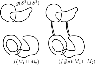
Figure 1. The componentwise embedded connected sum $\#$.

The described operation $\#$ defines a group structure on $E^{6}(S^{3})$ (or $E^{6}(S^{3}\sqcup S^{3})$) and an action of $E^{6}(S^{3})$ (or $E^{6}(S^{3}\sqcup S^{3})$) on $E^{6}(M_{1})$ (or $E^{6}(M_{1}\sqcup M_{2})$).

1.5. Definition of linked embedded connected sum $\#_{1}$, $\#_{2}$.

Let $f:M_{1}\sqcup M_{2}\rightarrow S^{6}$ and $g:S^{3}\rightarrow S^{6}$ be embeddings with disjoint images. For $k\in\{1,2\}$ connect $f(M_{k})$ with $g(S^{3})$ by a thin tube along an arc. Denote the obtained embedding $M_{1}\sqcup M_{2}\rightarrow S^{6}$ by $f\#_{k}g$. It is called a linked embedded connect sum of $f$ and $g$. Clearly, the embedding $f\#_{k}g$ depends on the choice of the arc and the tube, but we drop them from the notation. See Fig.2.

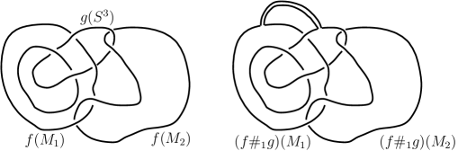
Figure 2. The linked embedded connected sum $\#_{1}$.

For the fixed embeddings $f$ and $g$ the isotopy class $[f\#_{k}g]$ is well defined, i.e., it does not depend on the choice of the arc or the tube. This can be proved analogously to [Sk15, Standardization Lemma, case $(p,q,m)=(0,3,6)$] (the independence on the choice of the arc also easily follows from the fact that the images of $f$ and $g$ have codimension greater than $2$).

1.6. Definition of the Whitney invariants $W$ and ${L}_{k}$.

Let $N$ be a closed connected orientable $3$-manifold. Our definition of the Whitney invariant $W:E^{6}(N)\rightarrow H_{1}(N)$ is equivalent to the one given in [Sk08a].

Let $f,f^{\prime}:N\rightarrow S^{6}$ be embeddings. Consider a general position homotopy $F:N\times I\rightarrow S^{6}\times I$ between $f$ and $f^{\prime}$. The Whitney invariant of the pair $(f,f^{\prime})$ is the homology class

$$W(f,f^{\prime}):=[\{x\in N\times I:|F^{-1}Fx|\geq 2\}]\in H_{1}(N\times I)=H_{1}(N)$$

which can be defined as in [Sk08b].

To define $W$ for a single embedding (as opposed to a pair $(f,f^{\prime})$ of embeddings) we need to choose some “base embedding”. Manifold $N$ is orientable, so it embeds into $S^{5}$, see [Hi61]. Let $f^{0}_{N}:N\rightarrow S^{6}$ be an embedding with the image in $S^{5}\subset S^{6}$. For any $f:N\rightarrow S^{6}$ denote

$$W(f):=W(f^{0}_{N},f).$$

We choose $f^{0}_{M_{1}}$ and $f^{0}_{M_{2}}$ so that their images lie in disjoint $6$-balls. Define

$$f^{0}:M_{1}\sqcup M_{2}\rightarrow S^{6}\text{\quad by the formula\quad}f^{0}=f^{0}_{M_{1}}\sqcup f^{0}_{M_{2}}.$$

Recall that for $k\in\{1,2\}$ and for an embedding $f:M_{1}\sqcup M_{2}\rightarrow S^{6}$ we earlier defined

$$W_{k}:E^{6}(M_{1}\sqcup M_{2})\rightarrow H_{1}(M_{k})\text{\quad by the formula\quad}W_{k}(f)=W(f|_{M_{k}}).$$

Let us now define ${L}_{1}$ and ${L}_{2}$. Let $f,f^{\prime}:M_{1}\sqcup M_{2}\rightarrow S^{6}$ be embeddings. Consider a general position homotopy $F:(M_{1}\sqcup M_{2})\times I\rightarrow S^{6}\times I$ between $f$ and $f^{\prime}$. The Whitney invariants ${L}_{1}$ and ${L}_{2}$ of the pair $(f,f^{\prime})$ are the homology classes

• ${L}_{1}(f,f^{\prime}):=[(F|_{M_{1}\times I})^{-1}(F(M_{1}\times I)\cap F(M_{2}\times I))]\in H_{1}(M_{1}),$

• ${L}_{2}(f,f^{\prime}):=[(F|_{M_{2}\times I})^{-1}(F(M_{1}\times I)\cap F(M_{2}\times I))]\in H_{1}(M_{2}).$

For $k\in\{1,2\}$ and any $f:M_{1}\sqcup M_{2}\rightarrow S^{6}$ denote

$${L}_{k}(f):={L}_{k}({f^{0}},f)\in H_{1}(M_{k}).$$

1.7. Proof of part (I) of Theorem 1.11.

The following claim is essentially proved (but not explicitly stated) in [Sk08a, “Construction of an arbitrary embedding $N\rightarrow{\mathbb{R}}^{6}$ from a fixed embedding $g:N\rightarrow{\mathbb{R}}^{5}$”]. For the readers convenience we present (a very similar) proof here. In the proof an later in the text we use the standard notation $V_{m,n}$ for the Stiefel manifold of $n$-frames in ${\mathbb{R}}^{m}$. All the framings (resp. frames) in the text are normal framings (resp. frames) compatible with orientation (in the case of framings).

Claim 1.19.

Let $f:M_{1}\sqcup M_{2}\rightarrow S^{6}$ be an embedding and $a\in H_{1}(M_{1})$ a homology class. Then there is an embedding $g:D^{4}\rightarrow S^{6}$ such that

• $g(S^{3})\cap{\rm Im}(f)=\emptyset,$

• $g(D^{4})\cap f(M_{2})=\emptyset,$

• $[(f|_{M_{1}})^{-1}g(D^{4})]=a.$

Proof.

Represent $a$ by an oriented circle in $M_{1}$ and denote the circle by the same letter. Consider a normal framing $\alpha$ of $f(a)$ in $f(M_{1})$. Extend it to a normal framing $\alpha,\beta$ of $f(a)$ in $S^{6}$, where $\beta$ is normal to $f(M_{1})$. The extension exists because $f(a)$ is unknotted in $S^{6}$ and so the obstruction to the existence of the extension is in $\pi_{1}(V_{5,2})=0$.

By general position there is a $2$-disk $\Delta$ in $S^{6}$ such that

• $\partial\Delta=f(a)$,

• ${\rm Int}\Delta\cap f(M_{1}\sqcup M_{2})=\emptyset,$

• the first vectors of $\beta$ “looks” inside of $\Delta$.

Denote by $\beta^{\prime}$ the normal $2$-frame of $f(a)$ made out of the last two vectors of $\beta$. Extend $\beta^{\prime}$ to a normal $2$-frame of $\Delta$. The extension exists because the obstruction to its existence is in $\pi_{1}(V_{4,2})=0$. The vectors of $\beta^{\prime}$ on $\Delta$ plus the vectors of $\beta$ on $\partial\Delta=f(a)$ give us an embedding $g:D^{4}\rightarrow D^{6}$ which is as required. ∎

Proof of part (I) of Theorem 1.11.

We need to prove that ${WL}$ is surjective.

Take any element $a^{\prime}\in H_{1}(M_{1})$ and any embedding $f:M_{1}\sqcup M_{2}\rightarrow S^{6}$. Denote $a:=a^{\prime}-W_{1}(f)$. Let $g:D^{4}\rightarrow S^{6}$ be an embedding given by Claim 1.19.

Consider the embedding $f^{\prime}:=f\#_{1}(g|_{S^{3}})$. There is a homotopy between $f^{\prime}$ and $f$ contracting $g(S^{3})$ along the disk $g(D^{4})$. By the definition of the Whitney invariants and by the construction of $g$, we have $W_{1}(f^{\prime})=W_{1}(f)+a=a^{\prime}$, and $W_{2}(f^{\prime})=W_{2}(f)$, ${L}_{1}(f^{\prime})={L}_{1}(f)$, ${L}_{2}(f^{\prime})={L}_{2}(f)$. So, we can change the value of the Whitney invariant $W_{1}$ of an embedding to any desired value $a^{\prime}$ without changing the other three Whitney invariants.

Similarly to the previous paragraph (take $f^{\prime\prime}:=f\#_{2}(g|_{S^{3}})$ instead of $f^{\prime}$) we can change the value of the Whitney invariant $L_{1}$ of an embedding to any desired value $a^{\prime}$ without changing the other three Whitney invariants.

Similarly to previous two paragraphs we can also change $W_{2}$ and ${L}_{2}$ in the same manner. So, ${WL}$ is surjective, because there exists at least one embedding $M_{1}\sqcup M_{2}\rightarrow S^{6}$ (for instance take $f^{0}$). ∎

1.8. Definition of the linking coefficients $\lambda_{1}$ and $\lambda_{2}$ and their relation to the Haefliger invariant $r$.

Let $g:S^{3}_{1}\sqcup S^{3}_{2}\rightarrow S^{6}$ be an embedding, where $S^{3}_{1}$ and $S^{3}_{2}$ are two copies of $S^{3}$. Choose an oriented disk $D^{3}_{g}\subset S^{6}$ intersecting $g(S^{3}_{2})$ transversally at a single point of positive sign. Identify $H_{2}(S^{6}\setminus gS^{3}_{2})$ with $\mathbb{Z}$ by identifying $[\partial D^{3}_{g}]\in H_{2}(S^{6}\setminus gS^{3}_{2})$ with $1\in{\mathbb{Z}}$. Identify $H_{2}(S^{2})$ with ${\mathbb{Z}}$ by choosing an orientation of $S^{2}$. Choose a homotopy equivalence $h:S^{6}\setminus gS^{3}_{2}\rightarrow S^{2}$ which induces the identity isomorphism in $H_{2}$. Define the first linking coefficient by the formula

$$\lambda_{1}(g):=[hg|_{S^{3}_{1}}]\in\pi_{3}(S^{2})={\mathbb{Z}},$$

where identification $\pi_{3}(S^{2})={\mathbb{Z}}$ identifies the homotopy class of the Hopf map with $1$. All the orientation preserving homotopy equivalences $S^{2}\rightarrow S^{2}$ are homotopic to each other, so $\lambda_{1}$ is well-defined.

The definition of the second linking coefficient $\lambda_{2}$ is analogous and is obtained by the exchange of the components,

$$\lambda_{2}(g):=\lambda_{1}(g^{\prime}),$$

where $g^{\prime}:S^{3}_{1}\sqcup S^{3}_{2}\rightarrow S^{6}$ is such that $g^{\prime}|_{S^{3}_{2}}=g|_{S^{3}_{1}}$ and $g^{\prime}|_{S^{3}_{1}}=g|_{S^{3}_{2}}$.

Let $A,B:S^{3}\rightarrow S^{6}$ be embeddings with disjoint images. For brevity denote

$$\lambda(A,B):=\lambda_{1}(A\sqcup B).$$

Informally, $\lambda(A,B)$ is the homotopy class of $A$ in the compliment to $B(S^{3})$.

The following lemma easily follows from the definition of $\lambda$.

Lemma 1.20.

Let $A,B,C:S^{3}\rightarrow S^{6}$ be embeddings with pairwise disjoint images. Then

$$\lambda(A\#B,C)=\lambda(A,C)+\lambda(A,B).$$

Remark 1.21.

Note that $\lambda(A,B\#C)$ is not necessarily equal to $\lambda(A,B)+\lambda(A,C)$ even if the images of $B$ and $C$ lie in pairwise disjoint $6$-balls. As an example one can take Borromean rings $A,B,C:S^{3}\rightarrow S^{6}$. Then $A\sqcup B\#C:S^{3}\sqcup S^{3}\rightarrow S^{6}$ is the Whitehead link with $\lambda(A,B\#C)=2\neq 0+0=\lambda(A,B)+\lambda(A,C)$, see [Sk15, Lemma 2.18].

For the proof of the following lemma see [Sk15, Lemma 2.16].

Lemma 1.22.

Let $A,B:S^{3}\rightarrow S^{6}$ be embeddings with disjoint images. Then

$$r(A\#B)=r(A)+r(B)+\frac{\lambda(A,B)+\lambda(B,A)}{2}.$$

In particular, $r(A\#B)=r(A)+r(B)$ if $A(S^{3})$ and $B(S^{3})$ lie in disjoint $6$-balls.

Remark 1.23.

The number $\frac{\lambda(A,B)+\lambda(B,A)}{2}$ is integer by Haefliger Theorem 1.5.

1.9. Proof of “PL” Theorem 1.18 modulo “smooth” Theorem 1.11.

For a piecewise smooth (PS) manifold $N$ denote by $E^{m}_{PS}(N)$ the set of PS isotopy classes of PS embeddings $N\rightarrow S^{m}$. The forgetful map $E^{m}_{PL}(N)\rightarrow E^{m}_{PS}(N)$ is a bijection, see [Ha67, §2.2]. Therefore, Theorem 1.18 can be restated in the PS category without any changes. For our convenience we shall prove the PS version of Theorem 1.18.

Let

$${\rm Fg}:E^{6}(M_{1}\sqcup M_{2})\rightarrow E^{6}_{PS}(M_{1}\sqcup M_{2})$$

be the forgetful map.

Lemma 1.24.

The forgetful map ${\rm Fg}$ has the following properties.

• ${\rm Fg}$ preserves the invariants $\lambda_{1}$, $\lambda_{2}$, and ${WL}$.

• ${\rm Fg}$ commutes with $\#$, i.e., ${\rm Fg}([f]\#[g])={\rm Fg}([f])\#{\rm Fg}([g])$ for any $[f]\in E^{6}(M_{1}\sqcup M_{2})$ and $[g]\in E^{6}_{PL}(S^{3}\sqcup S^{3})$.

• ${\rm Fg}$ is surjective.

• Suppose that ${\rm Fg}([f^{\prime}])={\rm Fg}([f])$ for some $[f],[f^{\prime}]\in E^{6}(M_{1}\sqcup M_{2})$. Then there is $[g]\in E^{6}(S^{3}\sqcup S^{3})$ such that $[f^{\prime}]=[f]\#[g]$ and that $[g]$ is unlinked, i.e., $\lambda_{1}(g)=\lambda_{2}(g)=0$.

Proof.

(1), (2) follow by the definitions of $\lambda_{1}$, $\lambda_{2}$, ${WL}$, and $\#$.

Let us prove (3). The obstruction to smoothing any PS embedding $M_{1}\sqcup M_{2}\rightarrow S^{6}$ lies in groups $H^{i+1}(M_{1}\sqcup M_{2};E^{i+3}(S^{i}))$ for $i=0,1,2$, see [Bo71, First paragraph of introduction], [Hu72, Proof of Lemma 7]. Since $E^{3}(S^{0})=E^{4}(S^{1})=E^{5}(S^{2})=0$, the obstruction vanishes.

It remains to prove (4). Let $F:(M_{1}\sqcup M_{2})\times I\rightarrow S^{6}\times I$ be a PS isotopy between $f$ and $f^{\prime}$. The only obstruction to smoothing $F$ is some cohomology class $a\in H^{4}((M_{1}\sqcup M_{2})\times I;E^{6}(S^{3}))\cong E^{6}(S^{3})\oplus E^{6}(S^{3})$. Choose an unlinked embedding $g:S^{3}\sqcup S^{3}\rightarrow S^{6}\times 0$ whose image is in a $6$-ball disjoint with the image of $F_{0}$ and such that $r_{1}(g)\oplus r_{2}(g)=a$. A PS embedding $G:D^{4}\sqcup D^{4}\rightarrow S^{6}\times I$ is obtained from $g$ by coning over two generic points. Then $F\#G$ is a PS concordance between $[f]\#[g]$ and $[f^{\prime}]$. By construction, $F\#G$ can be smoothed, therefore $[f^{\prime}]=[f]\#[g]$. Cf. [Sk08a, An alternative definition of the Kreck invariant]. ∎

Proof of Theorem 1.18.

Part (I) follows from Part (I) of Theorem 1.11 by (1) and (3). Part (II) follows from Part (II) of Theorem 1.11 by (1), (2), and (3). Part (III) follows from Part (II) of Theorem 1.11 by (1), (2), (3), and (4). ∎

2. Proof of the main theorem modulo lemmas.

2.1. Plan of the proof.

In this section we prove the main theorem modulo Surjectivity Lemma 2.3, Bijectivity Lemma 2.7, Preimage Lemma 2.9, Calculation Lemma 2.11, Linking Lemma 2.12, and Claim 2.8. All of these statements are proved later in the corresponding sections.

The plan of the proof is explained by the diagram in Fig.3. In this subsection we only give informal explanations. All the new objects and statements mentioned here or in the diagram are rigorously defined or stated later in this section.

We represent $M_{1}$ as the result of cutting several solid tori from $S^{3}$ and then pasting them back together by the diffeomorphism exchanging parallels with meridians. By $\widehat{M_{1}}$ we denote the compliment in $S^{3}$ to the solid tori, i.e., what is left of $S^{3}$ after cutting the tori and before pasting them back. The definition of $\widehat{M_{2}}$ is analogous.

By $\widehat{E}^{6}(\widehat{M_{1}}\sqcup\widehat{M_{2}})$ we denote the set of fixed on the boundary isotopy classes of proper embeddings $\widehat{M_{1}}\sqcup\widehat{M_{2}}\rightarrow D^{6}_{+}$. Given a representative of an element of $\widehat{E}^{6}(\widehat{M_{1}}\sqcup\widehat{M_{2}})$ we can extend it in two different “standard” ways to either an embedding $S^{3}\sqcup S^{3}\rightarrow S^{6}$ or an embedding $M_{1}\sqcup M_{2}\rightarrow S^{6}$. These extensions define the maps $\sigma_{R}$ and $\sigma$ in the diagram.

It turns out that the map $\sigma$ (and $\sigma_{R}$) is surjective, see the Surjectivity Lemma 2.3. I.e., any embedding $M_{1}\sqcup M_{2}\rightarrow S^{6}$ is isotopic to a so-called “standardized” embedding which is “standard” on the solid tori and which maps $\widehat{M_{1}}\sqcup\widehat{M_{2}}$ to $D^{6}_{+}$. The proof of Surjectivity Lemma 2.3 essentially repeats the proof of the first part of the Standardization Lemma in [Sk15] (which is stated in slightly less general case than we require).

Two isotopic “standardized” embeddings are not necessarily isotopic through “standardized” embeddings. This means that the map $\sigma$ is not bijective (and that the second part of the Standardization Lemma of [Sk15] fails in the dimensions we are working in). By studying the geometric obstruction to the “standardization” of an isotopy between two “standardized” embeddings we prove the Preimage Lemma 2.9.

The set $E^{6}(S^{3}\sqcup S^{3})$ is known and the maps $\sigma$ and $\sigma_{R}$ are surjective. Therefore we can classify the unknown set $E^{6}(M_{1}\sqcup M_{2})$ by describing the (not well-defined) “composition” $\sigma_{R}\circ\sigma^{-1}$. This task is accomplished by the Bijectivity, Preimage, and Calculation Lemmas 2.7, 2.9, and 2.11.

Figure 3. The diagram.

2.2. Definitions of $T_{n},P,\widehat{M_{k}},m,R$.

In this subsection we represent manifolds $M_{1}$ and $M_{2}$ as results of a surgery of $S^{3}$ on several embedded circles.

For any $n>0$ let

$$T_{n}:=\underbrace{S^{1}\times D^{2}\sqcup\ldots\sqcup S^{1}\times D^{2}}_{n}$$

be the disjoint union of $n$ copies of $S^{1}\times D^{2}$.

Let

$$R:S^{1}\times S^{1}\rightarrow S^{1}\times S^{1}$$

be the diffeomorphism exchanging the parallel with the meridian.

By [PS97, end of §12, beginning of §14] for each $k\in\{1,2\}$ there are $m_{k}>0$ and an embedding $P_{k}:T_{m_{k}}\rightarrow S^{3}$ such that

• the restriction of $P_{k}$ to each of $m_{k}$ connected components of $T_{m_{k}}$ is isotopic to the standard embedding $S^{1}\times D^{2}\rightarrow S^{3}$;

• if we denote

  $$\widehat{M_{k}}:=\text{\quad the closure of\quad}S^{3}\setminus P_{k}(T_{m_{k}})$$

  then

  $$M_{k}\cong\widehat{M_{k}}\underset{P_{k}(x)=R(x),x\in\partial T_{m_{k}}}{\bigcup}T_{m_{k}},$$

  (where “$\cong$” is a diffeomorphism).

For the rest of the text and for each $k\in\{1,2\}$ we replace $M_{k}$ with

$$\widehat{M_{k}}\underset{P_{k}(x)=R(x),x\in\partial T_{m_{k}}}{\bigcup}T_{m_{k}},$$

see Fig.4.

Figure 4. Manfiolds $M_{1}$ on the left and $S^{3}$ on the right.

Until the end of the text $k\in\{1,2\}$ and $1\leq i\leq m_{k}$. I.e., all the statements involving $k$ and/or $i$ are given for all $k\in\{1,2\}$ and $1\leq i\leq m_{k}$, unless specifically said otherwise.

2.3. Definitions of $P_{k,i},{\mathfrak{p}}_{k,i},h$.

Denote by $P_{k,i}$ the restriction of $P_{k}$ to the $i$-th connected component.

Fix an orientation of $S^{1}\times D^{2}$. Consider the meridian ${\mathfrak{m}}:=*\times S^{1}\subset S^{1}\times D^{2}$ with some orientation. Construct a normal framing of ${\mathfrak{m}}$ in the following way. The first vector of the framing “looks” inside the full-torus $S^{1}\times D^{2}$, the second vector of the framing is then determined uniquely by the compatibility with orientation. Denote the obtained framed circle by the same letter ${\mathfrak{m}}$.

Define framed circles ${\mathfrak{p}}_{k,i}\subset S^{3}$ by the formula

$${\mathfrak{p}}_{k,i}:=P_{k,i}R{\mathfrak{m}}\subset S^{3}.$$

Let $a\subset S^{3}$ be any framed $1$-submanifold. Shift $a$ slightly along the first vector of its framing and denote the obtained submanifold by $a^{\prime}$. The Hopf invariant $h(a)$ of $a$ is defined by the formula

$$h(a):={\rm lk}(a,a^{\prime})\in{\mathbb{Z}}.$$

The following claim easily follows from the definition of ${\mathfrak{p}}_{k,i}$.

Claim 2.1.

For any $k\in\{1,2\}$ and $1\leq i\leq m_{k}$ we have $h({\mathfrak{p}}_{k,i})=0$.

2.4. Definition of the set $\widehat{E}^{6}(\widehat{M_{1}}\sqcup\widehat{M_{2}})$.

Denote by $D^{6}_{+}$ and $D^{6}_{-}$ the northern and the southern hemispheres of $S^{6}$, respectively (the exact choice of the “north” and “south” poles is not important).

Let

$$s_{k}:\underbrace{D^{2}\times D^{4}\sqcup\ldots\sqcup D^{2}\times D^{4}}_{m_{k}}\rightarrow D^{6}_{-}$$

be an embedding such that

• its restriction to each $*\times D^{4}$ is isotopic to the standard proper embedding $D^{4}\rightarrow D^{6}_{-}$,

• there are pairwise disjoint $6$-balls $B_{k,i}\subset D^{6}_{-}$ such that the $s_{k}$-image of the $i$-th connected component lie in $B_{k,i}$.

We additionally demand that for every $1\leq i\leq m_{1}$, $1\leq j\leq m_{2}$ the balls $B_{1,i}$ and $B_{2,j}$ are disjoint.

Denote by $B^{\square}_{k,i}$ some tubular neighbourhood of $s_{k,i}(D^{2}\times D^{4})$ in $B_{k,i}$ modulo $s_{k,i}(D^{2}\times S^{3})$. Note that $B^{\square}_{k,i}$ is a manifold with “corners” diffeomorphic to $D^{2}\times D^{4}$.

We consider $S^{1}\times D^{2}$ as a submanidold of $D^{2}\times D^{4}$ where the inclusion $S^{1}\times D^{2}\subset D^{2}\times D^{4}$ is given by the obvious inclusions $S^{1}=\partial D^{2}\subset D^{2}$ and $D^{2}\subset D^{4}$.

Denote by $\widehat{E}^{6}(\widehat{M_{1}}\sqcup\widehat{M_{2}})$ the set of isotopy classes fixed on the boundary, of proper embeddings $\widehat{f}:\widehat{M_{1}}\sqcup\widehat{M_{2}}\rightarrow D^{6}_{+}$ such that

$$\widehat{f}\circ P_{k}|_{\partial T_{m_{k}}}=s_{k}|_{\partial T_{m_{k}}}$$

for each $k\in\{1,2\}$.

2.5. Definition of operations $\sigma$, $\sigma_{R}$ and the action $\#$.

For an embedding $\widehat{f}:\widehat{M_{1}}\sqcup\widehat{M_{2}}\rightarrow D^{6}_{+}$ such that $[\widehat{f}]\in\widehat{E}^{6}(\widehat{M_{1}}\sqcup\widehat{M_{2}})$ define

$$\sigma(\widehat{f}):M_{1}\sqcup M_{2}\rightarrow S^{6}\text{\quad by \quad}\sigma(\widehat{f})(x):=\begin{cases}\widehat{f}(x)\text{ if }x\in\widehat{M_{1}}\sqcup\widehat{M_{2}}\\ s_{k}(x)\text{ if }x\in(M_{k}\setminus\widehat{M_{k}})=T_{m_{k}}\end{cases},$$

see Fig.5.

Figure 5. Operation $\sigma$ (only $M_{1}$ is shown).

Denote by $s_{k,i}$ the restrictions of $s_{k}$ to the $i$-th connected component.

Let $A_{R}:D^{6}_{-}\rightarrow D^{6}_{-}$ be an orientation preserving diffeomorphism such that

• $A_{R}(B_{k,i})=B_{k,i}$,

• $A_{R}\circ s_{k,i}|_{S^{1}\times S^{1}}=s_{k,i}|_{S^{1}\times S^{1}}\circ R$.

Such a diffeomorphism exists because all embeddings $S^{1}\times S^{1}\rightarrow\partial D^{6}_{-}$ are isotopic and because smooth isotopies are ambient, see [Hu70, Theorem $2.1$].

Denote

$$s_{R,k}:=A_{R}\circ s_{k}\text{\quad and\quad}s_{R,k,i}:=A_{R}\circ s_{k,i}.$$

For an embedding $\widehat{f}:\widehat{M_{1}}\sqcup\widehat{M_{2}}\rightarrow D^{6}_{+}$ such that $[\widehat{f}]\in\widehat{E}^{6}(\widehat{M_{1}}\sqcup\widehat{M_{2}})$ define

$$\sigma_{R}(\widehat{f}):M_{1}\sqcup M_{2}\rightarrow S^{6}\text{\quad by \quad}\sigma(\widehat{f})(x):=\begin{cases}\widehat{f}(x)\text{ if }x\in\widehat{M_{1}}\sqcup\widehat{M_{2}}\\ s_{R,k}(x)\text{ if }x\in(M_{k}\setminus\widehat{M_{k}})=T_{m_{k}}\end{cases},$$

see Fig.6.

Figure 6. Operation $\sigma_{R}$ (only $M_{1}$ is shown).

Clearly, if $[\widehat{f}]=[\widehat{f^{\prime}}]$ for some other embedding $\widehat{f^{\prime}}$, then $[\sigma(\widehat{f})]=[\sigma(\widehat{f^{\prime}})]$ and $[\sigma_{R}(\widehat{f})]=[\sigma_{R}(\widehat{f^{\prime}})]$. Therefore $\sigma$ and $\sigma_{R}$ induce well-defined maps

$$E^{6}(S^{3}\sqcup S^{3})\xleftarrow{\sigma_{R}}\widehat{E}^{6}(\widehat{M_{1}}\sqcup\widehat{M_{2}})\xrightarrow{\sigma}E^{6}(M_{1}\sqcup M_{2}),$$

which we denote by the same letters.

Note that in our notation $\sigma(\widehat{f})$ is an embedding while $\sigma([\widehat{f}])$ is an isotopy class.

The group $E^{6}(S^{3}\sqcup S^{3})$ acts on each of the sets $E^{6}(S^{3}\sqcup S^{3})$, $\widehat{E}^{6}(\widehat{M_{1}}\sqcup\widehat{M_{2}})$, and $E^{6}(M_{1}\sqcup M_{2})$ via the component-wise connected sum $\#$. The action on $\widehat{E}^{6}(\widehat{M_{1}}\sqcup\widehat{M_{2}})$ is defined analogously to the action on $E^{6}(S^{3}\sqcup S^{3})$ or $E^{6}(M_{1}\sqcup M_{2})$.

The following claim easily follows from the definitions of $\sigma$, $\sigma_{R}$, and the embedded connected sum action $\#$.

Claim 2.2 ($\#$-commutativity).

The embedded connected sum action $\#$ commutes with $\sigma$ and $\sigma_{R}$. I.e., for any isotopy classes $[\widehat{f}]\in\widehat{E}^{6}(\widehat{M_{1}}\sqcup\widehat{M_{2}})$ and $[g]\in E^{6}(S^{3}\sqcup S^{3})$ we have $\sigma([\widehat{f}]\#[g])=\sigma([\widehat{f}])\#[g]$ and $\sigma_{R}([\widehat{f}]\#[g])=\sigma_{R}([\widehat{f}])\#[g]$.

Lemma 2.3 (Surjectivity).

Maps $\sigma$ and $\sigma_{R}$ are surjective.

2.6. Definition of the Whitney invariants $\widehat{W}_{k}$, $\widehat{{L}}_{k}$ of proper embeddings.

The definition of

$$\widehat{W}_{k},\widehat{{L}}_{k}:\widehat{E}^{6}(\widehat{M_{1}}\sqcup\widehat{M_{2}})\rightarrow H_{1}(\widehat{M_{k}})$$

is analogous to the definition of

$$W_{k},{L}_{k}:E^{6}(M_{1}\sqcup M_{2})\rightarrow H_{1}(M_{k}).$$

One needs only to replace “homotopy” by “homotopy relative to the boundary” and define a “base embedding” $\widehat{f}^{0}:\widehat{M_{1}}\sqcup\widehat{M_{2}}\rightarrow D^{6}_{+}$. To do the latter we choose some $[\widehat{f}^{0}]\in\widehat{E}^{6}(\widehat{M_{1}}\sqcup\widehat{M_{2}})$ such that $\sigma([\widehat{f}^{0}])=[{f^{0}}]$. The existence of such $[\widehat{f}^{0}]$ is guaranteed by Surjectivity Lemma 2.3.

The following claim easily follows from the definition of $\widehat{{L}}_{k}$.

Claim 2.4.

Take any $k\in\{1,2\}$ and $[\widehat{f}]\in\widehat{E}^{6}(\widehat{M_{1}}\sqcup\widehat{M_{2}})$. Let $\Delta_{k}\subset D^{6}_{+}$ be a proper submanifold “with corners”, $\partial\Delta_{k}=\widehat{f}(\widehat{M_{k}})\cup(\partial\Delta_{k}\cap\partial D^{6}_{+})$. Suppose that $\Delta_{k}$ is disjoint with $\widehat{f}(\partial\widehat{M_{3-k}})\subset\partial D^{6}_{+}$. Then

$$\widehat{L}_{3-k}(\widehat{f})=[(\widehat{f}^{-1})\Delta_{k}]\in H_{1}(\widehat{M_{3-k}}).$$

For brevity, denote

$$\widehat{{WL}}:=\widehat{W}_{1}\times\widehat{{L}}_{1}\times\widehat{W}_{2}\times\widehat{{L}}_{2}.$$

The map

$$H_{1}(\widehat{M_{1}})\times H_{1}(\widehat{M_{1}})\times H_{1}(\widehat{M_{2}})\times H_{1}(\widehat{M_{2}})\rightarrow H_{1}({M_{1}})\times H_{1}({M_{1}})\times H_{1}({M_{2}})\times H_{1}({M_{2}})$$

in the diagram is induced by the inclusions $\widehat{M_{1}}\subset M_{1}$ and $\widehat{M_{2}}\subset M_{2}$.

Our choice of the “base element” $[\widehat{f}^{0}]\in\widehat{E}^{6}(\widehat{M_{1}}\sqcup\widehat{M_{2}})$ implies the following two claims.

Claim 2.5.

For any $k\in\{1,2\}$, $[\widehat{f}]\in\widehat{E}^{6}(\widehat{M_{1}}\sqcup\widehat{M_{2}})$ and $[f]:=\sigma([\widehat{f}])$ the homology classes $\widehat{W}_{k}(\widehat{f})$ and $W_{k}(f)$ can be represented by the same $1$-submanifold in $\widehat{M_{k}}$. Likewise, the homology classes $\widehat{{L}}_{k}(\widehat{f})$ and ${L}_{k}(f)$ can be represented by the same $1$-submanifold in $\widehat{M_{k}}$.

Claim 2.6.

The square in the diagram above commutes.

2.7. Proof of part (II) of Theorem 1.11.

Lemma 2.7 (Bijectivity).

For any $x\in H_{1}(\widehat{M_{1}})\times H_{1}(\widehat{M_{1}})\times H_{1}(\widehat{M_{2}})\times H_{1}(\widehat{M_{2}})$ the restriction $\sigma_{R}|_{\widehat{{WL}}^{-1}(x)}$ is a bijection.

Claim 2.8.

Let $[f],[f^{\prime}]\in E^{6}(M_{1}\sqcup M_{2})$ be isotopy classes such that ${WL}(f)={WL}(f^{\prime})$. Then there are isotopy classes $[\widehat{f}],[\widehat{f^{\prime}}]\in\widehat{E}^{6}(\widehat{M_{1}}\sqcup\widehat{M_{2}})$ such that $\sigma([\widehat{f}])=[f]$, $\sigma([\widehat{f^{\prime}}])=[f^{\prime}]$, and $\widehat{{WL}}(\widehat{f})=\widehat{{WL}}(\widehat{f^{\prime}})$.

Proof of part (II) of Theorem 1.11.

Let $[f],[f^{\prime}]\in E^{6}(M_{1}\sqcup M_{2})$ be isotopy classes such that ${WL}(f)={WL}(f^{\prime})$. To complete the proof we need to find an embedding $g:S^{3}\sqcup S^{3}\rightarrow S^{6}$ such that $[f^{\prime}]\#[g]=[f]$.

Let $[\widehat{f}],[\widehat{f^{\prime}}]\in\widehat{E}^{6}(\widehat{M_{1}}\sqcup\widehat{M_{2}})$ be the isotopy classes whose existence is guaranteed by Claim 2.8. By Haefliger Theorem 1.5 there is an embedding $g:S^{3}\sqcup S^{3}\rightarrow D^{6}_{+}$ such that

$$\sigma_{R}([\widehat{f^{\prime}}])\#[g]=\sigma_{R}([\widehat{f}]).$$

By $\#$-commutativity Claim 2.2 we get

$$\sigma_{R}([\widehat{f^{\prime}}]\#[g])=\sigma_{R}([\widehat{f}]).$$

Clearly, $\widehat{{WL}}([\widehat{f^{\prime}}]\#[g])=\widehat{{WL}}([\widehat{f^{\prime}}])$, so by Bijectivity Lemma 2.7 we have

$$[\widehat{f^{\prime}}]\#[g]=[\widehat{f}].$$

So,

$$[\widehat{f^{\prime}}]\#[g]=[\widehat{f}]\text{\quad}\Rightarrow\text{\quad}\sigma([\widehat{f^{\prime}}]\#[g])=\sigma([\widehat{f}])\overset{(1)}{\text{\quad}\Rightarrow\text{\quad}}\\ \overset{(1)}{\text{\quad}\Rightarrow\text{\quad}}\sigma([\widehat{f^{\prime}}])\#[g]=\sigma([\widehat{f}])\overset{(2)}{\text{\quad}\Rightarrow\text{\quad}}[f^{\prime}]\#[g]=[f],$$

where (1) follows by the $\#$-commutativity Claim 2.2 and (2) follows from the choice of $[\widehat{f}]$ and $[\widehat{f^{\prime}}]$. We get that $g$ is as required. ∎

2.8. Definition of $\omega$.

Define

$$\omega_{k,i}:S^{3}\rightarrow S^{6}\text{\quad by the formula \quad}\omega_{k,i}:=s_{k,i}|_{0\times S^{3}},$$

see Fig.7.

Figure 7. The circle $f({\mathfrak{p}}_{1,1})$, the sphere $\omega_{1,1}(S^{3})$, and the disk $\Delta_{\omega,1,1}$.

2.9. Multiple linked embedded connected sum.

Take any $[\widehat{f}]\in\widehat{E}^{6}(\widehat{M_{1}}\sqcup\widehat{M_{2}})$ and $g:S^{3}\rightarrow\partial D^{6}_{+}$ such that the images of $\widehat{f}$ and $g$ are disjoint. For $k\in\{1,2\}$ we shall write

$$\widehat{f}\#_{k}g$$

meaning $\widehat{f}\#_{k}g^{\prime}$ – the linked embedded connected sum of $f$ with some embedding $g^{\prime}:S^{3}\rightarrow{\rm Int}D^{6}_{+}$ obtained from $g$ by a slight shift into the interior of $D^{6}_{+}$. This agreement guarantees that $[\widehat{f}\#_{k}g]\in\widehat{E}^{6}(\widehat{M_{1}}\sqcup\widehat{M_{2}})$.

For any integer $a$ we denote

• $\widehat{f}\#_{k}ag:=\widehat{f}\underbrace{\#_{k}g\#_{k}g\ldots\#_{k}g}_{a},\text{\quad if \quad}a>0,$

• $\widehat{f}\#_{k}ag:=\widehat{f}\#_{k}(-a)(-g),\text{\quad if \quad}a<0,$

• $\widehat{f}\#_{k}ag:=\widehat{f}\text{\quad if \quad}a=0.$

Here $-g:S^{3}\rightarrow\partial D^{6}_{+}$ is an embedding such that ${\rm Im}(-g)={\rm Im}(g)$ and $[g]\#[-g]$ is trivial considered as an isotopy class of an embedding $S^{3}\rightarrow S^{6}$.

2.10. Proof of part (III) of Theorem 1.11.

The following lemma allows us to describe the preimage of $\sigma$.

Lemma 2.9 (Preimage).

For any $[\widehat{f}],[\widehat{f}^{\prime}]\in\widehat{E}^{6}(\widehat{M_{1}}\sqcup\widehat{M_{2}})$ we have that $\sigma([\widehat{f}])=\sigma([\widehat{f}^{\prime}])$ if and only if

$$[\widehat{f}^{\prime}]=[\widehat{f}\underset{i=1}{\overset{m_{1}}{\#_{1}}}a_{i}\omega_{1,i}\underset{i=1}{\overset{m_{1}}{\#_{2}}}b_{i}\omega_{i,1}\underset{j=1}{\overset{m_{2}}{\#_{2}}}c_{j}\omega_{2,j}\underset{j=1}{\overset{m_{2}}{\#_{1}}}d_{j}\omega_{2,j}]$$

for some integers $a_{i}$, $b_{i}$, $c_{j}$, and $d_{j}$.

Remark 2.10.

In other words, the lemma states that $\sigma([\widehat{f}])=\sigma([\widehat{f}^{\prime}])$ if and only if $[\widehat{f}^{\prime}]$ can be obtained from $[\widehat{f}]$ by several operations of the form

• $[\widehat{f}]\to[\widehat{f}\#_{1}\pm\omega_{1,i}],$

• $[\widehat{f}]\to[\widehat{f}\#_{2}\pm\omega_{1,i}],$

• $[\widehat{f}]\to[\widehat{f}\#_{1}\pm\omega_{2,j}],$

• $[\widehat{f}]\to[\widehat{f}\#_{2}\pm\omega_{2,j}].$

where $1\leq i\leq m_{1}$ and $1\leq j\leq m_{2}$.

Proof of the “if part” of Preimage Lemma 2.9.

The remark above makes the “if” part obvious. For instance, there is an isotopy between $\sigma(\widehat{f}\#_{1}\pm\omega_{1,i})$ and $\sigma(\widehat{f})$ which “drags” the sphere $\omega_{1,i}(S^{3})$ along the disk $s_{1,i}(0\times D^{4})$. This is indeed an isotopy because the disk $s_{1,i}(0\times D^{4})$ is disjoint with ${\rm Im}(\sigma(\widehat{f}))$, see Fig.7 for the case $i=1$. ∎

For a homology class $a\in H_{1}(\widehat{M_{k}})$ we denote by ${\rm lk}({\mathfrak{p}}_{k,i},a)$ the linking number of ${\mathfrak{p}}_{k,i}\subset\partial\widehat{M_{k}}$ and any oriented $1$-submanifold of ${\rm Int}\widehat{M_{k}}\subset S^{3}$ representing $a$. Clearly, this linking number is well defined, i.e., do not depend on the choice of the representative.

Denote by $[{\mathfrak{p}}_{k,i}]$ the respective homology class in $H_{1}(\widehat{M_{k}})$.

Let $\widehat{f}$ be a proper embedding such that $[\widehat{f}]\in\widehat{E}^{6}(\widehat{M_{1}}\sqcup\widehat{M_{2}})$. Denote

$${l}_{k,i}(\widehat{f}):=\lambda(\omega_{k,i},(\sigma_{R}\widehat{f})_{k}),$$

where $(\sigma_{R}\widehat{f})_{k}$ is the restriction of $\sigma_{R}\widehat{f}:S^{3}\sqcup S^{3}\rightarrow S^{6}$ to the $k$-th connected component of its domain.

Lemma 2.11 (Calculation).

Suppose that $[\widehat{f}]\in\widehat{E}^{6}(\widehat{M_{1}}\sqcup\widehat{M_{2}})$, $1\leq i\leq m_{1}$, and $1\leq j\leq m_{2}$.

In the first column of the table is an embedding $\widehat{f}^{\prime}$. In the first row are symbols denoting different isotopy invariants.

In each cell of the columns “$\lambda_{1}$” to “$r_{2}$” is the difference of the corresponding invariant of $\sigma_{R}(\widehat{f}^{\prime})$ and $\sigma_{R}(\widehat{f})$.

In each cell of the columns “$\widehat{W}_{1}$” to “$\widehat{{L}}_{2}$” is the difference of the corresponding invariant of $\widehat{f}^{\prime}$ and $\widehat{f}$.

$\widehat{f}^{\prime}$ $\lambda_{1}$ $\lambda_{2}$ $r_{1}$ $r_{2}$ $\widehat{W}_{1}$ $\widehat{W}_{2}$ $\widehat{{L}}_{1}$ $\widehat{{L}}_{2}$ $\widehat{f}\#_{1}\omega_{1,i}$ $0$ $2{\rm lk}(\widehat{{L}}_{1}\widehat{f},{\mathfrak{p}}_{1,i})$ $\frac{{l}_{1,i}(\widehat{f})}{2}$ $0$ $[{\mathfrak{p}}_{1,i}]$ $0$ $0$ $0$ $\widehat{f}\#_{2}\omega_{1,i}$ $2{\rm lk}(\widehat{{L}}_{1}\widehat{f},{\mathfrak{p}}_{1,i})$ ${l}_{1,i}(\widehat{f})$ $0$ $0$ $0$ $0$ $[{\mathfrak{p}}_{1,i}]$ $0$ $\widehat{f}\#_{2}\omega_{2,j}$ $2{\rm lk}(\widehat{{L}}_{2}\widehat{f},{\mathfrak{p}}_{2,j})$ $0$ $0$ $\frac{{l}_{2,j}(\widehat{f})}{2}$ $0$ $[{\mathfrak{p}}_{2,j}]$ $0$ $0$ $\widehat{f}\#_{1}\omega_{2,j}$ ${l}_{2,j}(\widehat{f})$ $2{\rm lk}(\widehat{{L}}_{2}\widehat{f},{\mathfrak{p}}_{2,j})$ $0$ $0$ $0$ $0$ $0$ $[{\mathfrak{p}}_{2,j}]$

We shall refer to the cells of the table by their respective row number and column title. E.g., cell (1,$\lambda_{1}$) contains $0$ and means that $\lambda_{1}(\sigma_{R}(\widehat{f}\#_{1}\omega_{1,i}))-\lambda_{1}(\sigma_{R}(\widehat{f}))=0$; cell (3,$\widehat{W}_{2}$) contains $[{\mathfrak{p}}_{2,j}]$ and means that $\widehat{W}_{2}(\widehat{f}\#_{2}\omega_{2,j})-\widehat{W}_{2}(\widehat{f})=[{\mathfrak{p}}_{2,j}]$; etc.

Lemma 2.12 (Linking).

For any $k\in\{1,2\}$, integers $a_{i}$, and isotopy class $[\widehat{f}]\in\widehat{E}^{6}(\widehat{M_{1}}\sqcup\widehat{M_{2}})$ the following implication holds

$$\overset{m_{k}}{\underset{i=1}{\Sigma}}a_{i}[{\mathfrak{p}}_{k,i}]=0\text{\quad}\Rightarrow\text{\quad}\overset{m_{k}}{\underset{i=1}{\Sigma}}a_{i}{l}_{k,i}(\widehat{f})=\overset{m_{k}}{\underset{i=1}{\Sigma}}2{\rm lk}({\mathfrak{p}}_{k,i},\widehat{W}_{k}\widehat{f}).$$

Denote by $[{\mathfrak{p}}_{k,i}]_{\partial\widehat{M_{k}}}$ the respective homology class in $H_{1}(\partial\widehat{M_{k}})$.

Consider the following part of the Mayer–Vietoris long exact sequence

$$H_{2}(M_{k})\xrightarrow{\partial}H_{1}(\partial\widehat{M_{k}})\xrightarrow{i_{\widehat{M_{k}}},i_{T_{m_{k}}}}H_{1}(\widehat{M_{k}})\oplus H_{k}(T_{m_{1}}),$$

where the maps $i_{\widehat{M_{k}}}$ and $i_{T_{m_{k}}}$ are induced by the inclusions $\partial\widehat{M_{k}}\subset\widehat{M_{k}}$ and $\partial\widehat{M_{k}}\subset T_{m_{k}}$.

Claim 2.13.

The image of $\partial:H_{2}(M_{k})\rightarrow H_{1}(\partial\widehat{M_{k}})$ is the subgroup of $H_{1}(\partial\widehat{M_{k}})$ consisting of all linear combinations of the form $\underset{i=1}{\overset{m_{k}}{\Sigma}}a_{i}[{\mathfrak{p}}_{k,i}]_{\partial\widehat{M_{k}}}$ such that $\underset{i=1}{\overset{m_{k}}{\Sigma}}a_{i}[{\mathfrak{p}}_{k,i}]=0\in H_{1}(\widehat{M_{k}})$.

Proof.

From the construction of $M_{k}$ it is clear, that ${\rm Ker}(i_{T_{m_{k}}})$ consists exclusively of all linear combinations of $[{\mathfrak{p}}_{k,i}]_{\partial\widehat{M_{k}}}$.

By the definition, $i_{\widehat{M_{k}}}([{\mathfrak{p}}_{k,i}]_{\partial\widehat{M_{k}}})=[{\mathfrak{p}}_{k,i}]$, so any linear combination of the form $\underset{i=1}{\overset{m_{k}}{\Sigma}}a_{i}[{\mathfrak{p}}_{k,i}]_{\partial\widehat{M_{k}}}$ is in ${\rm Ker}(i_{\widehat{M_{k}}})$ if and only if $\underset{i=1}{\overset{m_{k}}{\Sigma}}a_{i}[{\mathfrak{p}}_{k,i}]=0\in H_{1}(\widehat{M_{k}})$.

Now the claim follows from the exactness of the Mayer–Vietoris sequence above. ∎

Claim 2.14.

Take any $\alpha\in H_{2}(M_{k})$. By Claim 2.13, $\partial\alpha=\underset{i=1}{\overset{m_{k}}{\Sigma}}a_{i}[{\mathfrak{p}}_{k,i}]_{\partial\widehat{M_{k}}}$ for some integers $a_{i}$. Then for any $[\widehat{f}]\in\widehat{E}^{6}(\widehat{M_{1}}\sqcup\widehat{M_{2}})$ and $[f]:=\sigma([\widehat{f}])$

• ${L}_{k}f\cap\alpha=\underset{i=1}{\overset{m_{k}}{\Sigma}}a_{i}{\rm lk}(\widehat{{L}}_{k}\widehat{f},{\mathfrak{p}}_{k,i})$,

• $W_{k}f\cap\alpha=\underset{i=1}{\overset{m_{k}}{\Sigma}}a_{i}\frac{{l}_{k,i}}{2}$.

Proof.

(I). Follows from

$${L}_{k}f\cap\alpha=\widehat{{L}}_{k}\widehat{f}\cap\alpha={\rm lk}(\widehat{{L}}_{k}\widehat{f},\partial\alpha)=\underset{i=1}{\overset{m_{k}}{\Sigma}}a_{i}{\rm lk}(\widehat{{L}}_{k}\widehat{f},{\mathfrak{p}}_{k,i}).$$

The first equality holds by Claim 2.5. The second equality holds by the definition of ${\rm lk}$.

(II). Follows from

$$W_{k}f\cap\alpha=\widehat{W}_{k}\widehat{f}\cap\alpha={\rm lk}(\widehat{W}_{k}\widehat{f},\partial\alpha)=\underset{i=1}{\overset{m_{k}}{\Sigma}}a_{i}{\rm lk}(\widehat{W}_{k}\widehat{f},{\mathfrak{p}}_{k,i})=\underset{i=1}{\overset{m_{k}}{\Sigma}}a_{i}\frac{{l}_{k,i}}{2}.$$

The first equality holds by Claim 2.5. The second equality holds by the definition of ${\rm lk}$. The last equality holds by Linking Lemma 2.12, which we can apply because $\overset{m_{k}}{\underset{i=1}{\Sigma}}a_{i}[{\mathfrak{p}}_{k,i}]=0$ by Claim 2.13. ∎

Proof of the “if” statement in part (III) of Theorem 1.11.

Until the end of the proof identify $E^{6}(S^{3}\sqcup S^{3})$ with $\widetilde{{\mathbb{Z}}^{4}}$ by the isomorphism $\lambda_{1}\times\lambda_{2}\times r_{1}\times r_{2}$.

Let $f:M_{1}\sqcup M_{2}\rightarrow S^{6}$ be an embedding. Let $g:S^{3}\sqcup S^{3}\rightarrow S^{6}$ be an embedding such that $[g]\in{\rm Stab}_{f}\subset\widetilde{{\mathbb{Z}}^{4}}$. We need to prove that $[f]=[f]\#[g]$.

By the definition of ${\rm Stab}_{f}$, there are $\alpha,\beta\in H_{2}(M_{1})$ and $\gamma,\delta\in H_{2}(M_{2})$ such that $[g]=[g_{\alpha}]+[g_{\beta}]+[g_{\gamma}]+[g_{\delta}]$, where

• $[g_{\alpha}]=(0,2{L}_{1}f\cap\alpha,W_{1}f\cap\alpha,0)\in\widetilde{{\mathbb{Z}}^{4}}$,

• $[g_{\beta}]=(2{L}_{1}f\cap\beta,2W_{1}f\cap\beta,0,0)\in\widetilde{{\mathbb{Z}}^{4}}$,

• $[g_{\gamma}]=(2{L}_{2}f\cap\gamma,0,0,W_{2}f\cap\gamma)\in\widetilde{{\mathbb{Z}}^{4}}$,

• $[g_{\delta}]=(2W_{2}f\cap\delta,2{L}_{2}f\cap\delta,0,0)\in\widetilde{{\mathbb{Z}}^{4}}$.

It is enough to prove that $[f]=[f]\#[g_{\alpha}]$, $[f]=[f]\#[g_{\beta}]$, $[f]=[f]\#[g_{\gamma}]$, and $[f]=[f]\#[g_{\delta}]$. We shall only prove the first equality because the proofs of others are analogous.

By Claim 2.13, there are integers $a_{i}$ such that $\partial\alpha=\underset{i=1}{\overset{m_{1}}{\Sigma}}a_{i}[{\mathfrak{p}}_{1,i}]_{\partial\widehat{M_{1}}}$. By Surjection Lemma 2.3, there is an embedding $\widehat{f}:\widehat{M_{1}}\sqcup\widehat{M_{2}}\rightarrow D^{6}_{+}$ such that $\sigma([\widehat{f}])=[f]$. Denote

$$[\widehat{f^{\prime}}]:=[\widehat{f}\underset{i=1}{\overset{m_{1}}{\#_{1}}}a_{i}\omega_{1,i}].$$

Now the equality $[f]=[f]\#[g_{\alpha}]$, which we want to prove, follows from

$$[f]=\sigma([\widehat{f}])\overset{(1)}{=}\sigma([\widehat{f^{\prime}}])\overset{(2)}{=}\sigma([\widehat{f}]\#[g_{\alpha}])\overset{(3)}{=}\sigma([\widehat{f}])\#[g_{\alpha}]=[f]\#[g_{\alpha}],$$

where (1) follows by Preimage Lemma 2.9 and (3) follows by $\#$-commutativity Claim 2.2. Equation (2) follows from

$$\widehat{{WL}}([\widehat{f^{\prime}}])\overset{(4)}{=}\widehat{{WL}}([\widehat{f}]\#[g_{\alpha}])$$

and

$$\sigma_{R}([\widehat{f^{\prime}}])\overset{(5)}{=}\sigma_{R}([\widehat{f}]\#[g_{\alpha}])$$

by Bijection Lemma 2.7. It remains to prove (4) and (5).

Now (4) follows from

$$\widehat{{WL}}([\widehat{f^{\prime}}])-\widehat{{WL}}([\widehat{f}]\#[g_{\alpha}])=\widehat{{WL}}([\widehat{f^{\prime}}])-\widehat{{WL}}([\widehat{f}])=\underset{i=1}{\overset{m_{1}}{\Sigma}}a_{i}[{\mathfrak{p}}_{1,i}]=0,$$

where the second equality follows by the definiton of $[\widehat{f^{\prime}}]$ and Calculation Lemma 2.11, cells (1,$\widehat{W}_{1}$-$\widehat{{L}}_{2}$). The last equality holds by Claim 2.13.

And (5) follows from

$$\sigma_{R}([\widehat{f^{\prime}}])-\sigma_{R}([\widehat{f}]\#[g_{\alpha}])=\sigma_{R}([\widehat{f^{\prime}}])-\sigma_{R}([\widehat{f}])-[g_{\alpha}]=\\ =(0,2\underset{i=1}{\overset{m_{1}}{\Sigma}}a_{i}{\rm lk}(\widehat{{L}}_{1}\widehat{f},{\mathfrak{p}}_{1,i}),\underset{i=1}{\overset{m_{1}}{\Sigma}}a_{i}\frac{{l}_{1,i}(\widehat{f})}{2},0)-[g_{\alpha}]=\\ =(0,2{L}_{1}f\cap\alpha,W_{1}f\cap\alpha,0)-(0,2{L}_{1}f\cap\alpha,W_{1}f\cap\alpha,0)=0\in\widetilde{{\mathbb{Z}}^{4}},$$

where the second equality holds by Calculation Lemma 2.11, cells (1,$\lambda_{1}$-$r_{2}$). The third equality holds by Claim 2.14 and by the definition of $[g_{\alpha}]$. ∎

Proof of the “only if” statement in part (III) of Theorem 1.11.

Until the end of the proof identify $E^{6}(S^{3}\sqcup S^{3})$ with $\widetilde{{\mathbb{Z}}^{4}}$ by the isomorphism $\lambda_{1}\times\lambda_{2}\times r_{1}\times r_{2}$.

Let $f:M_{1}\sqcup M_{2}\rightarrow S^{6}$ be an embedding. Let $g:S^{3}\sqcup S^{3}\rightarrow S^{6}$ be an embedding such that $[f]=[f]\#[g]$. We need to prove that $[g]\in{\rm Stab}_{f}$.

By Surjection Lemma 2.3, there is an embedding $\widehat{f}:\widehat{M_{1}}\sqcup\widehat{M_{2}}\rightarrow D^{6}_{+}$ such that $\sigma([\widehat{f}])=[f]$. By $\#$-commutativity Claim 2.2, $\sigma([\widehat{f}]\#[g])=\sigma([\widehat{f}])\#[g]=[f]\#[g]=[f]$.

So both $[\widehat{f}]$ and $[\widehat{f}]\#[g]$ are $\sigma$-preimages of $[f]$. By Preimage Lemma 2.9, there are integers $a_{i}$, $b_{i}$, $c_{j}$, and $d_{j}$ such that

$$[\widehat{f}]\#[g]=[\widehat{f}\underset{i=1}{\overset{m_{1}}{\#_{1}}}a_{i}\omega_{1,i}\underset{i=1}{\overset{m_{1}}{\#_{2}}}b_{i}\omega_{i,1}\underset{j=1}{\overset{m_{2}}{\#_{2}}}c_{j}\omega_{2,j}\underset{j=1}{\overset{m_{2}}{\#_{1}}}d_{j}\omega_{2,j}].$$

Clearly $\widehat{{WL}}([\widehat{f}])=\widehat{{WL}}([\widehat{f}]\#[g])$. From that, the equation above, and Calculation Lemma 2.11 (last four columns of the table) we get that

$$\underset{i=1}{\overset{m_{1}}{\Sigma}}a_{i}[{\mathfrak{p}}_{1,i}]=\underset{i=1}{\overset{m_{1}}{\Sigma}}b_{i}[{\mathfrak{p}}_{1,i}]=\underset{j=1}{\overset{m_{2}}{\Sigma}}c_{j}[{\mathfrak{p}}_{2,j}]=\underset{j=1}{\overset{m_{2}}{\Sigma}}d_{j}[{\mathfrak{p}}_{2,j}]=0.$$

By Claim 2.13, there is $\alpha\in H_{2}(M_{1})$ such that $\partial\alpha=\underset{i=1}{\overset{m_{1}}{\Sigma}}a_{i}[{\mathfrak{p}}_{1,i}]_{\partial\widehat{M_{1}}}$. The definitions of $\beta\in H_{2}(M_{1})$, $\gamma,\delta\in H_{2}(M_{2})$ are analogous but with $(a_{i},{\mathfrak{p}}_{1,i})$ replaced by $(b_{i},{\mathfrak{p}}_{1,i})$, $(c_{j},{\mathfrak{p}}_{2,j})$, and $(d_{j},{\mathfrak{p}}_{2,j})$, respectively.

The statement of the theorem now follows from

$$\sigma_{R}([\widehat{f}])+[g]\overset{(1)}{=}\sigma_{R}([\widehat{f}]\#[g])=\\ =\sigma_{R}([\widehat{f}\underset{i=1}{\overset{m_{1}}{\#_{1}}}a_{i}\omega_{1,i}\underset{i=1}{\overset{m_{1}}{\#_{2}}}b_{i}\omega_{i,1}\underset{j=1}{\overset{m_{2}}{\#_{2}}}c_{j}\omega_{2,j}\underset{j=1}{\overset{m_{2}}{\#_{1}}}d_{j}\omega_{2,j}])\overset{(2)}{=}\\ \overset{(2)}{=}\sigma_{R}([\widehat{f}\underset{i=1}{\overset{m_{1}}{\#_{1}}}a_{i}\omega_{1,i}\underset{i=1}{\overset{m_{1}}{\#_{2}}}b_{i}\omega_{i,1}\underset{j=1}{\overset{m_{2}}{\#_{2}}}c_{j}\omega_{2,j}])+(2W_{2}f\cap\delta,2{L}_{2}f\cap\delta,0,0)\overset{(3)}{=}\\ \overset{(3)}{=}\sigma_{R}([\widehat{f}\underset{i=1}{\overset{m_{1}}{\#_{1}}}a_{i}\omega_{1,i}\underset{i=1}{\overset{m_{1}}{\#_{2}}}b_{i}\omega_{i,1}])+(2{L}_{2}f\cap\gamma,0,0,W_{2}f\cap\gamma)+(2W_{2}f\cap\delta,2{L}_{2}f\cap\delta,0,0)\overset{(4)}{=}\\ \overset{(4)}{=}\sigma_{R}([\widehat{f}\underset{i=1}{\overset{m_{1}}{\#_{1}}}a_{i}\omega_{1,i}])+(2{L}_{1}f\cap\beta,2W_{1}f\cap\beta,0,0)+\\ (2{L}_{2}f\cap\gamma,0,0,W_{2}f\cap\gamma)+(2W_{2}f\cap\delta,2{L}_{2}f\cap\delta,0,0)\overset{(5)}{=}\\ \overset{(5)}{=}\sigma_{R}([\widehat{f}])+(0,2{L}_{1}f\cap\alpha,W_{1}f\cap\alpha,0)+(2{L}_{1}f\cap\beta,2W_{1}f\cap\beta,0,0)+\\ +(2{L}_{2}f\cap\gamma,0,0,W_{2}f\cap\gamma)+(2W_{2}f\cap\delta,2{L}_{2}f\cap\delta,0,0)\\ \Downarrow\\ [g]=(0,2{L}_{1}f\cap\alpha,W_{1}f\cap\alpha,0)+(2{L}_{1}f\cap\beta,2W_{1}f\cap\beta,0,0)+\\ +(2{L}_{2}f\cap\gamma,0,0,W_{2}f\cap\gamma)+(2W_{2}f\cap\delta,2{L}_{2}f\cap\delta,0,0)\in{\rm Stab}_{f}.$$

Here (1) follows by $\#$-commutativity Claim 2.2. It remains to prove (2-5). Let us only prove (5) as (2-4) are proved analogously. Equation (5) is equivalent to

$$\sigma_{R}([\widehat{f}\underset{i=1}{\overset{m_{1}}{\#_{1}}}a_{i}\omega_{1,i}])-\sigma_{R}([\widehat{f}])=(0,2{L}_{1}f\cap\alpha,W_{1}f\cap\alpha,0)\in\widetilde{{\mathbb{Z}}^{4}},$$

which in turn follows by Calculation Lemma 2.11, cells (1, $\lambda_{1}$-$r_{2}$), and by Claim 2.13. ∎

3. Proof of Surjectivity, Bijectivity, and Preimage Lemmas 2.3, 2.7, 2.9.

Throughout this section we denote by $q_{k,i}$ the circle $S^{1}\times 0$ in the $i$-th connected component of $T_{m_{k}}$, see Fig.8.

Figure 8. The circle $q_{1,1}$ represented by a pair of squares.

3.1. Proof of Surjectivity Lemma 2.3.

Proof of Surjectivity Lemma 2.3..

We only prove that the map $\sigma$ is surjective. The map $\sigma_{R}$ is surjective by an analogous argument.

Choose an arbitrary embedding $f:M_{1}\sqcup M_{2}\rightarrow S^{6}$. By general position, there are $2$-disks $\Delta_{k,i}$ in $S^{6}$ (see Fig.9), such that

• $\partial\Delta_{k,i}=f(q_{k,i})$,

• interiors of all $\Delta_{k,i}$ are pairwise disjoint and are disjoint with $f(M_{1}\sqcup M_{2})$.

Figure 9. Proof of Surjectivity Lemma 2.3.

The restriction of $f$ to the $i$-th component of $T_{m_{k}}$ can be extended to an embedding $F_{k,i}:D^{2}\times D^{4}\rightarrow S^{6}$ such that (see Fig.9)

• $F_{k,i}(D^{2}\times 0)=\Delta_{k,i}$,

• ${\rm Im}(F_{k,i})\cap{\rm Im}(f)=F_{k,i}(S^{1}\times D^{2})$,

• images of all the $F_{k,i}$ are pairwise disjoint.

Indeed, the obstruction to an extension to $D^{2}\times D^{2}$ is in $\pi_{1}(V_{4,2})=0$. Having $F_{k,i}$ already defined on $D^{2}\times D^{2}$ we can extend it to $D^{2}\times D^{4}$ without any obstructions.

Let $N_{k,i}$ be a tubular neighbourhood modulo $F_{k,i}(D^{2}\times S^{3})$ of $F_{k,i}(D^{2}\times D^{4})$ (see Fig.9). We can choose all $N_{k,i}$ to be pairwise disjoint and such that $N_{k,i}\cap f(\widehat{M_{1}}\sqcup\widehat{M_{2}})=F_{k,i}(S^{1}\times D^{2})$. By construction, $F_{k,i}:D^{2}\times D^{4}\rightarrow N_{k,i}$ is isotopic to the composition of $s_{k,i}:D^{2}\times D^{4}\rightarrow B^{\square}_{k,i}$ with some diffeomorphism $B^{\square}_{k,i}\rightarrow N_{k,i}$, see the right part of Fig.9. There is a $6$-ball $B$ containing all of $N_{k,i}$, interior of $B$ being also disjoint with $f(\widehat{M_{1}}\sqcup\widehat{M_{2}})$.

Apply an ambient isotopy of $S^{6}$ which maps $B$ to $D^{6}_{-}$, each $N_{k,i}$ to $B^{\square}_{k,i}$, and each $F_{k,i}$ to $s_{k,i}$.

Denote by $f^{\prime}$ the result obtained from $f$ by the isotopy. By construction, $f^{\prime}$ is in the image of $\sigma$. ∎

3.2. Proof of the “only if” part of Preimage Lemma 2.9.

We need the following Claim to prove the “only if” part of Preimage Lemma 2.9.

Claim 3.1.

Let $[\widehat{f}],[\widehat{f^{\prime}}]\in\widehat{E}^{6}(\widehat{M_{1}}\sqcup\widehat{M_{2}})$ be isotopy classes. Suppose that embeddings $\sigma(\widehat{f})$ and $\sigma(\widehat{f^{\prime}})$ are isotopic. Then there is a concordance between $\sigma(\widehat{f})$ and $\sigma(\widehat{f^{\prime}})$ fixed on $T_{m_{1}}\sqcup T_{m_{2}}$.

Proof.

Denote $f:=\sigma(\widehat{f})$ and $f^{\prime}:=\sigma(\widehat{f^{\prime}})$. By the definition of $\sigma$, we have that $f|_{T_{m_{1}}\sqcup T_{m_{2}}}=f^{\prime}|_{T_{m_{1}}\sqcup T_{m_{2}}}=s_{1}\sqcup s_{2}$.

Clearly, it suffices to find a concordance between $f$ and $f^{\prime}$ fixed on some tubular neighbourhood of each circle $q_{k,i}$.

Let $F:(M_{1}\sqcup M_{2})\times I\rightarrow S^{6}$ be an isotopy between $f$ and $f^{\prime}$. By general position, $F$ is isotopic relative to the boundary to some concordance $F^{\prime}$ fixed on each $q_{k,i}$.

At each point of $F^{\prime}(q_{1,1}\times I)$ identify with ${\mathbb{R}}^{5}$ the normal to $F^{\prime}(q_{1,1}\times I)$ space in $S^{6}\times I$. The restriction of $F^{\prime}$ to a small tubular neighbourhood of $q_{1,1}\times I$ gives us then a map $u:S^{1}\times I\rightarrow V_{5,2}$. We can choose the identification so that $u$ is constant on $S^{1}\times\partial I$.

Let $\bar{u}:\frac{S^{1}\times I}{S^{1}\times\partial I}\rightarrow V_{5,2}$ be the quotient map. Space $\frac{S^{1}\times I}{S^{1}\times\partial I}$ is homotopically equivalent to $S^{2}\vee S^{1}$. From $\pi_{2}(V_{5,2})=\pi_{1}(V_{5,2})=0$ it follows that $\bar{u}$ is null-homotopic. Therefore $u$ is homotopic relative $S^{1}\times\partial I$ to the constant map.

It implies that isotopying $F^{\prime}$ in a small tubular neighbourhood of $q_{1,1}\times I$ we can make $F^{\prime}$ constant on this tubular neighbourhood. Doing this for all $k,i$ we get the required concordance. ∎

Proof of the “only if” part of Preimage Lemma 2.9..

Suppose that $\sigma([\widehat{f}])=\sigma([\widehat{f}^{\prime}])$ for some $[\widehat{f}],[\widehat{f}^{\prime}]\in\widehat{E}^{6}(\widehat{M_{1}}\sqcup\widehat{M_{2}})$. Denote $f:=\sigma(\widehat{f})$ and $f^{\prime}:=\sigma(\widehat{f}^{\prime})$.

By Claim 3.1, there is a concordance $F$ between $f$ and $f^{\prime}$, fixed on $T_{m_{1}}\sqcup T_{m_{2}}$.

Denote $\Delta_{k,i}:=s_{k,i}(D^{2}\times 0)$. Disks $\Delta_{k,i}$ are pairwise disjoint, $\partial\Delta_{k,i}=f(q_{k,i})=f^{\prime}(q_{k,i})=F_{t}(q_{k,i})$ for every $t\in I$, the interior of each $\Delta_{k,i}$ is disjoint with $s_{1}(T_{m_{1}})\sqcup s_{2}(T_{m_{2}})$.

For any $n$ and any two general position submanifolds $A,B\subset S^{n}$, ${\dim A}+{\dim B}=n$, denote by $\#|A\cap B|$ the algebraic number of points of intersection $A\cap B$. For each $\Delta_{k,i}$ denote by $\mathaccent 28695{\Delta_{k,i}}$ its interior.

For $1\leq i\leq m_{1}$, $1\leq j\leq m_{2}$ define

$$a_{i}:=\#|\mathaccent 28695{\Delta_{1,i}}\times I\cap F(M_{1}\times I)|,\text{\quad}b_{i}:=\#|\mathaccent 28695{\Delta_{1,i}}\times I\cap F(M_{2}\times I)|,$$

$$c_{j}:=\#|\mathaccent 28695{\Delta_{2,j}}\times I\cap F(M_{2}\times I)|,\text{\quad}d_{j}:=\#|\mathaccent 28695{\Delta_{2,j}}\times I\cap F(M_{1}\times I)|.$$

Denote

$$\widehat{f^{\prime\prime}}:=\widehat{f}\underset{i=1}{\overset{m_{1}}{\#_{1}}}a_{i}\omega_{1,i}\underset{i=1}{\overset{m_{1}}{\#_{2}}}b_{i}\omega_{i,1}\underset{j=1}{\overset{m_{2}}{\#_{2}}}c_{j}\omega_{2,j}\underset{j=1}{\overset{m_{2}}{\#_{1}}}d_{j}\omega_{2,j},$$

and

$$f^{\prime\prime}:=\sigma(\widehat{f^{\prime\prime}}).$$

It remains to prove that $[\widehat{f^{\prime}}]=[\widehat{f^{\prime\prime}}]$.

By construction, there is an isotopy $F^{\prime\prime}$ between $f$ and $f^{\prime\prime}$ which “drags” spheres $\omega_{1,i}$ and $\omega_{2,j}$ along pairwise disjoint embedded disks $s_{1,i}(0\times D^{4})$ and $s_{2,j}(0\times D^{4})$ for all $i$ and $j$. Isotopy $F^{\prime\prime}$ is fixed on $T_{m_{1}}\sqcup T_{m_{2}}$. We have that

$$\#|\mathaccent 28695{\Delta_{1,i}}\times I\cap F^{\prime\prime}(M_{1}\times I)|=a_{i},\text{\quad}\#|\mathaccent 28695{\Delta_{1,i}}\times I\cap F^{\prime\prime}(M_{2}\times I)|=b_{i},$$

$$\#|\mathaccent 28695{\Delta_{2,j}}\times I\cap F^{\prime\prime}(M_{2}\times I)|=c_{j},\text{\quad}\#|\mathaccent 28695{\Delta_{2,j}}\times I\cap F^{\prime\prime}(M_{1}\times I)|=d_{j}.$$

Consider now the concordance $H:=-F\cup F^{\prime\prime}$ between $f^{\prime}$ and $f^{\prime\prime}$. By construction, $H$ is fixed on $T_{m_{1}}\sqcup T_{m_{2}}$ and

$$\#|\mathaccent 28695{\Delta_{1,i}}\times I\cap H(M_{1}\times I)|=0,\text{\quad}\#|\mathaccent 28695{\Delta_{1,i}}\times I\cap H(M_{2}\times I)|=0,$$

$$\#|\mathaccent 28695{\Delta_{2,j}}\times I\cap H(M_{2}\times I)|=0,\text{\quad}\#|\mathaccent 28695{\Delta_{2,j}}\times I\cap H(M_{1}\times I)|=0.$$

So, using the Whitney trick ([Mi65, Theorem $6.6$]), we can isotope $H$, changing it only on $(\widehat{M_{1}}\sqcup\widehat{M_{2}})\times{\rm Int}I$, to some concordance $H^{\prime}$ whose image is disjoint with each $\mathaccent 28695{\Delta_{1,i}}\times I$ and $\mathaccent 28695{\Delta_{2,j}}\times I$.

Now we can “push” the image of $H^{\prime}$ away from each $\Delta_{1,i}\times I$ along the vectors of the normal framing of $\Delta_{1,i}\times I$ given by the embeddings $s_{1,i}(D^{2}\times D^{4})$ (recall that $s_{k,i}(D^{2}\times 0)=\Delta_{k,i}$ by the definition of $\Delta_{k,i}$). Likewise we can “push” the image of $H^{\prime}$ away from each $\Delta_{2,j}\times I$.

We obtain a new concordance $H^{\prime\prime}$ between $f^{\prime}$ and $f^{\prime\prime}$ such that $H^{\prime\prime}((\widehat{M_{1}}\sqcup\widehat{M_{2}})\times I)\subset D^{6}_{+}\times I$. The restriction of $H^{\prime\prime}$ to $(\widehat{M_{1}}\sqcup\widehat{M_{2}})\times I$ is a concordance between $\widehat{f^{\prime}}$ and $\widehat{f^{\prime\prime}}$ in $D^{6}_{+}$ fixed on the boundary. In codimension at least $3$ concordance implies isotopy, see [Hu70, Theorem $2.1$], therefore $[\widehat{f^{\prime}}]=[\widehat{f^{\prime\prime}}]$. ∎

3.3. Proof of Bijectivity Lemma 2.7.

To prove the Bijectivity Lemma 2.7 we shall need the following analogue of Preimage Lemma 2.9.

For all $k\in\{1,2\}$ and $1\leq i\leq m_{k}$ define

$$\omega_{R,k,i}:S^{3}\rightarrow S^{6}\text{\quad by the formula \quad}\omega_{R,k,i}:=s_{R,k,i}|_{0\times S^{3}}.$$

Lemma 3.2 (Preimage’).

For any $[\widehat{f}],[\widehat{f}^{\prime}]\in\widehat{E}^{6}(\widehat{M_{1}}\sqcup\widehat{M_{2}})$ we have that $\sigma_{R}([\widehat{f}])=\sigma_{R}([\widehat{f}^{\prime}])$ if and only if

$$[\widehat{f}^{\prime}]=[\widehat{f}\underset{i=1}{\overset{m_{1}}{\#_{1}}}a_{i}\omega_{R,1,i}\underset{i=1}{\overset{m_{1}}{\#_{2}}}b_{i}\omega_{R,i,1}\underset{j=1}{\overset{m_{2}}{\#_{2}}}c_{j}\omega_{R,2,j}\underset{j=1}{\overset{m_{2}}{\#_{1}}}d_{j}\omega_{R,2,j}]$$

for some integers $a_{i}$, $b_{i}$, $c_{j}$, and $d_{j}$.

The proof of Preimage’ Lemma 3.2 is analogous to the proof of Preimage Lemma 2.9.

Proof of Bijectivity Lemma 2.7..

Let us first prove that the restriction $\sigma_{R}|_{\widehat{{WL}}^{-1}(x)}$ is surjective.

Choose any $[g]\in E^{6}(S^{3}\sqcup S^{3})$. The map $\widehat{{WL}}$ is surjective, which is proved analogously to the surjectivity of ${WL}$ (part (I) of Theorem 1.11). So, we can choose some $[\widehat{f}]\in\widehat{E}^{6}(\widehat{M_{1}}\sqcup\widehat{M_{2}})$ such that $\widehat{{WL}}(\widehat{f})=x$.

There is an isotopy class $[g^{\prime}]\in E^{6}(S^{3}\sqcup S^{3})$ such that $\sigma_{R}([\widehat{f}])\#[g^{\prime}]=[g]$. Then $\sigma_{R}([\widehat{f}]\#[g^{\prime}])=[g]$ and $\widehat{{WL}}([\widehat{f}]\#[g^{\prime}])=\widehat{{WL}}([\widehat{f}])=x$.

Let us now prove that the restriction $\sigma_{R}|_{\widehat{{WL}}^{-1}(x)}$ is injective. Let $[\widehat{f}],[\widehat{f}^{\prime}]\in\widehat{E}^{6}(\widehat{M_{1}}\sqcup\widehat{M_{2}})$ be some isotopy classes such that $\sigma_{R}([\widehat{f}])=\sigma_{R}([\widehat{f}^{\prime}])$ and $\widehat{{WL}}(\widehat{f})=\widehat{{WL}}(\widehat{f}^{\prime})=x$.

By Preimage’ Lemma 3.2, we have that

$$[\widehat{f}^{\prime}]=[\widehat{f}\underset{i=1}{\overset{m_{1}}{\#_{1}}}a_{i}\omega_{R,1,i}\underset{i=1}{\overset{m_{1}}{\#_{2}}}b_{i}\omega_{R,i,1}\underset{j=1}{\overset{m_{2}}{\#_{2}}}c_{j}\omega_{R,2,j}\underset{j=1}{\overset{m_{2}}{\#_{1}}}d_{j}\omega_{R,2,j}]$$

for some integers $a_{i}$, $b_{i}$, $c_{j}$, and $d_{j}$.

Similarly to ${\mathfrak{m}}$ and ${\mathfrak{p}}_{k,i}$ denote

$${\mathfrak{p}}:=S^{1}\times*\subset S^{1}\times D^{2}$$

and

$${\mathfrak{m}}_{k,i}:=P_{k,i}R{\mathfrak{p}}.$$

By $[{\mathfrak{m}}_{1,i}]$ we denote the corresponding homology classes in $\widehat{M_{1}}$ (analogously to $[{\mathfrak{p}}_{1,i}]$). Let us compute ${\rm lk}(\underset{i=1}{\overset{m_{1}}{\Sigma}}a_{i}[{\mathfrak{m}}_{1,i}],P_{1,1}q_{1,1})$ in two ways.

Circles ${\mathfrak{m}}_{k,i}$ are meridians of the pairwise disjoint embedded solid tori $P_{k,i}(S^{1}\times D^{2})\subset S^{3}$ and $P_{1,1}q_{1,1}$ is the parallel of the solid torus $P_{1,1}(S^{1}\times D^{2})\subset S^{3}$. Therefore,

$${\rm lk}(\underset{i=1}{\overset{m_{1}}{\Sigma}}a_{i}[{\mathfrak{m}}_{1,i}],P_{1,1}q_{1,1})=a_{1}.$$

By the analogue of Calculation Lemma 2.11 (cell (1, $W_{1}$)), we have that

$$\widehat{W}_{1}(\widehat{f^{\prime}})=\widehat{W}_{1}(\widehat{f})+\underset{i=1}{\overset{m_{1}}{\Sigma}}a_{i}[{\mathfrak{m}}_{1,i}].$$

Since $\widehat{W}_{1}(\widehat{f^{\prime}})=\widehat{W}_{1}(\widehat{f})$, it follows that $\underset{i=1}{\overset{m_{1}}{\Sigma}}a_{i}[{\mathfrak{m}}_{1,i}]=0\in H_{1}(\widehat{M_{1}})$. Circle $P_{1,1}q_{1,1}\subset S^{3}$ is disjoint with $\widehat{M_{1}}\subset S^{3}$, therefore

$${\rm lk}(\underset{i=1}{\overset{m_{1}}{\Sigma}}a_{i}[{\mathfrak{m}}_{1,i}],P_{1,1}q_{1,1})=0.$$

Combining the last two paragraphs we get that $a_{1}=0$. By the same argument, $a_{i}=b_{j}=c_{j}=d_{j}=0$ for all $i,j$, meaning that $[\widehat{f}]=[\widehat{f^{\prime}}]$. ∎

4. Proof of Calculation Lemma 2.11.

For the proof of Calculation Lemma 2.11 we use Lemma 4.1 which can be seen as an alternative definition of the linking coefficients $\lambda_{1}$ and $\lambda_{2}$. We shall also need additional Claim 4.2.

4.1. Definition of framed intersections and preimages.

Let $A,B\subset S^{n}$ be submanifodls in general position. Suppose that $B$ is framed. Then the framed intersection $A\cap B$ is a framed submanifold of $A$. The framing of $A\cap B\subset A$ is obtained by the projection of the framing of $B$ onto the tangent space of $A$ and subsequent Gram-Schmidt orthonormalising process.

Let $f:A\rightarrow S^{n}$ be an embedding and let $a\subset f(A)$ be a framed submanifold of $f(A)$. Then $f^{-1}(a)$ is called a framed preimage of $a$. The framing of $f^{-1}(a)$ is the $df^{-1}$-image of the framing of $a$.

Recall that $h$ denotes the Hopf invariant of a framed $1$-submanifold of $S^{3}$.

Lemma 4.1.

Let $g:S^{3}_{1}\sqcup S^{3}_{2}\rightarrow S^{6}$ be an embedding, where $S^{3}_{1}$ and $S^{3}_{2}$ are two distinct copies of $S^{3}$. Suppose that the restriction of $g$ to each connected component is trivial. Let $\Delta_{1}$, $\Delta_{2}$ be framed embedded disks in general position bounded by $gS^{3}_{1}$ and $gS^{3}_{2}$, respectively. Then

$$\lambda_{1}(g)=h(g^{-1}(gS^{3}_{1}\cap\Delta_{2}))\text{\quad and\quad}\lambda_{2}(g)=h(g^{-1}(gS^{3}_{2}\cap\Delta_{1})).$$

Proof.

We only prove the first claim as the second one is analogous. Clearly, $\Delta_{2}$ is the preimage of a regular point of some homotopy equivalence $S^{6}\setminus gS^{3}_{2}\rightarrow S^{2}$. Therefore $gS^{3}_{1}\cap\Delta_{2}$ is the preimage of the same point under the restriction of this homotopy equivalence to $gS^{3}_{1}$. The first claim of the lemma now holds by the definition of $\lambda_{1}$. ∎

4.2. Definition of $\Delta_{\omega,k,i}$.

Let $\Delta_{\omega,k,i}\subset\partial D^{6}_{-}$ be an embedded framed $4$-disk bounded by $\omega_{k,i}(S^{3})$ and such that for any $[\widehat{f}]\in\widehat{E}^{6}(\widehat{M_{1}}\sqcup\widehat{M_{2}})$

$$\widehat{f}^{-1}(\widehat{f}\widehat{M_{k}}\cap\Delta_{\omega,k,i})=(\sigma_{R}\widehat{f})^{-1}(\sigma_{R}\widehat{f}(S^{3}_{k})\cap\Delta_{\omega,k,i})={\mathfrak{p}}_{k,i},$$

where $S^{3}_{k}$ is the $k$-th component of the domain of $\sigma_{R}f$, see Fig.7. Here the “$=$” signs mean the equality of both sides as framed submanifolds. The first equality holds by definition of $\sigma_{R}$ and the second equality is a part of the definition of $\Delta_{\omega,k,i}$.

Claim 4.2.

For any $k\in\{1,2\}$, $1\leq i\leq m_{k}$ there exist a disk $\Delta_{\omega,k,i}\subset\partial D^{6}_{-}$ satisfying the properties above.

The claim is made obvious by Fig.7.

4.3. Proof of Calculation Lemma 2.11.

We shall prove the first two rows of the table, the proof for the second two rows is analogous. Without a loss of generality we may assume that $i=1$. For brevity denote $\omega:=\omega_{1,1}$ and $\Delta_{\omega}:=\Delta_{\omega,1,1}$.

Without a loss of generality we may also assume that the restriction of $\sigma_{R}\widehat{f}$ to the second component is trivial. Indeed, for any $g:S^{3}\rightarrow D^{6}_{+}$ whose image is far away from the images of $\widehat{f}$ and $\widehat{f^{\prime}}$ we may substitute $\widehat{f}$ and $\widehat{f^{\prime}}$ by $\widehat{f}\#_{2}g$ and $\widehat{f^{\prime}}\#_{2}g$, respectively, without changing any of the table entries. By choosing $g$ appropriately we can always make the restriction of $\sigma_{R}\widehat{f}$ to the second component trivial.

Let $F_{k}:S^{3}\rightarrow S^{6}$ be the restriction of $\sigma_{R}f$ to the $k$-th component. Embedding $F_{2}$ is trivial by the argument in the previous paragraph.

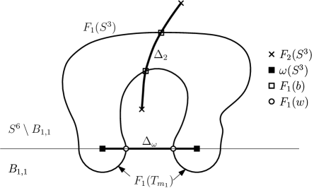
Figure 10. Proof of Calculation Lemma 2.11.

Consider some embedded framed $4$-disk $\Delta_{2}$ in the complement to $B_{1,1}$ bounded by $F_{2}(S^{3})$. Denote

$$w:=F_{1}^{-1}(F_{1}(S^{3})\cap\Delta_{\omega}),$$

$$b:=F_{1}^{-1}(F_{1}(S^{3})\cap\Delta_{2}).$$

Both $w$ and $b$ are framed $1$-submanifolds of $S^{3}$. Recall that $w={\mathfrak{p}}_{1,1}$ as a framed submanifold by Claim 4.2.

We prove the second row of the table first.

Cell (2, $\lambda_{1}$). In this cell we need to compute $\lambda_{1}(\sigma_{R}(\widehat{f}\#_{2}\omega_{1,1}))-\lambda_{1}(\sigma_{R}(\widehat{f}))=\lambda(F_{1},F_{2}\#\omega)-\lambda(F_{1},F_{2})$.

The disks $\Delta_{2}$ and $\Delta_{\omega}$ are disjoint by construction. So there is a framed embedded disk $\Delta_{F_{2}\#\omega}$, bounded by $(F_{2}\#\omega)(S^{3})$ and such that $F_{1}S^{3}\cap\Delta_{F_{2}\#\omega}=(F_{1}S^{3}\cap\Delta_{2})\sqcup(F_{1}S^{3}\cap\Delta_{\omega})$. So by Lemma 4.1 we have

$$\lambda(F_{1},F_{2}\#\omega)-\lambda(F_{1},F_{2})=h(F_{1}^{-1}(F_{1}\cap\Delta_{F_{2}\#\omega}))-h(F_{1}^{-1}(F_{1}\cap\Delta_{2}))=\\ =h(b\sqcup w)-h(b)=h(b)+h(w)+2{\rm lk}(b,w)-h(b)=h(w)+2{\rm lk}(b,w)=\\ =h({\mathfrak{p}}_{1,1})+2{\rm lk}(b,{\mathfrak{p}}_{1,1})=0+2{\rm lk}(b,{\mathfrak{p}}_{1,1})=2{\rm lk}(\widehat{{L}}_{1}\widehat{f},{\mathfrak{p}}_{1,1}).$$

The equation before the last holds because $h({\mathfrak{p}}_{1,1})=0$ by Claim 2.1. The last equation holds by Claim 2.4 (take $\Delta_{2}\cap D^{6}_{+}$ as “$\Delta$” in the statement of the claim. Clearly, $\Delta_{2}\cap D^{6}_{+}$ satisfies the necessary condition by construction.).

Cell (2, $\lambda_{2}$). In this cell we need to compute $\lambda_{2}(\sigma_{R}(\widehat{f}\#_{2}\omega_{1,1}))-\lambda_{2}(\sigma_{R}(\widehat{f}))=\lambda(F_{2}\#\omega,F_{1})-\lambda(F_{2},F_{1})$.

We have

$$\lambda(F_{2}\#\omega,F_{1})-\lambda(F_{2},F_{1})=\lambda(F_{2},F_{1})+\lambda(\omega,F_{1})-\lambda(F_{2},F_{1})=\lambda(\omega,F_{1})={l}_{1,1}(\widehat{f}).$$

The first equation holds by Lemma 1.20. The last equation is the definition of ${l}_{1,1}(\widehat{f})$.

Cell (2, $r_{1}$). In this cell we have $r_{1}(\sigma_{R}(\widehat{f}\#_{2}\omega_{1,1}))-r_{1}(\sigma_{R}(\widehat{f}))=0$ because the restrictions of $\sigma_{R}(\widehat{f}\#_{2}\omega_{1,1})$ and $\sigma_{R}(\widehat{f})$ to the first connected component are the same by the definition of $\#_{2}$.

Cell (2, $r_{2}$). By construction $\omega$ is trivial and the images of $\omega$ and $F_{2}$ lie in disjoint $6$-balls. So in this cell we have $r_{2}(\sigma_{R}(\widehat{f}\#_{2}\omega_{1,1}))-r_{2}(\sigma_{R}(\widehat{f}))=r(F_{2}\#\omega)-r(F_{2})=0$.

Cells (2,${\widehat{W}_{1}}$-${\widehat{{L}}_{2}}$). Clearly, there is a homotopy between $\widehat{f}\#_{2}\omega$ and $\widehat{f}$ which shrinks $\omega(S^{3})$ along the disk $\Delta_{\omega}$. The disk $\Delta_{\omega}$ is disjoint with the image of $\widehat{M_{2}}$ and the homotopy is the identity on $\widehat{M_{1}}$. So $\widehat{f^{\prime}}=\widehat{f}\#_{2}\omega$ and $\widehat{f}$ differ at only one Whitney invariant out of four, namely

$$\widehat{{L}}_{1}(\widehat{f}\#_{2}\omega)-\widehat{{L}}_{1}(\widehat{f})=\widehat{f}^{-1}[\widehat{f}(\widehat{M_{1}})\cap\Delta_{\omega}]=[w]=[{\mathfrak{p}}_{1,1}].$$

Cell (1, $\lambda_{1}$). In this cell we need to compute $\lambda_{1}(\sigma_{R}(\widehat{f}\#_{1}\omega_{1,1}))-\lambda_{1}(\sigma_{R}(\widehat{f}))=\lambda(F_{1}\#\omega,F_{2})-\lambda(F_{1},F_{2})$.

We have

$$\lambda(F_{1}\#\omega,F_{2})-\lambda(F_{1},F_{2})=\lambda(F_{1},F_{2})+\lambda(\omega,F_{2})-\lambda(F_{1},F_{2})=\lambda(\omega,F_{2})=0.$$

The first equation holds by Lemma 1.20. The last equation holds because the images of $\omega$ and $F_{2}$ lie in disjoint $6$-balls.

Cell (1, $\lambda_{2}$). In this cell we need to compute $\lambda_{2}(\sigma_{R}(\widehat{f}\#_{1}\omega_{1,1}))-\lambda_{2}(\sigma_{R}(\widehat{f}))=\lambda(F_{2},F_{1}\#\omega)-\lambda(F_{2},F_{1})$.

By Lemma 1.22 we have

$$2r(F_{1}\#F_{2}\#\omega)=\lambda(F_{2},F_{1}\#\omega)+,$$

$$2r(F_{1}\#F_{2}\#\omega)=\lambda(F_{2}\#\omega,F_{1})+\lambda(F_{1},F_{2}\#\omega)+2r(F_{2}\#\omega)+2r(F_{1}).$$

So

$$\lambda(F_{2},F_{1}\#\omega)=\lambda(F_{2}\#\omega,F_{1})+\lambda(F_{1},F_{2}\#\omega)+2r(F_{2}\#\omega)+2r(F_{1})-\lambda(F_{1}\#\omega,F_{2})-2r(F_{2})-2r(F_{1}\#\omega).$$

Applying Lemma 1.20 and Lemma 1.22 we get

$$\lambda(F_{2},F_{1}\#\omega)=\lambda(F_{2}\#\omega,F_{1})+\lambda(F_{1},F_{2}\#\omega)+2r(F_{2}\#\omega)+2r(F_{1})-\lambda(F_{1}\#\omega,F_{2})-2r(F_{2})-2r(F_{1}\#\omega)=\\ =\lambda(F_{2},F_{1})+\lambda(\omega,F_{1})+\lambda(F_{1},F_{2}\#\omega)+2r(F_{2})+2r(\omega)+\lambda(F_{2},\omega)+\lambda(\omega,F_{2})+2r(F_{1})-\\ -\lambda(F_{1},F_{2})-\lambda(\omega,F_{2})-2r(F_{2})-2r(F_{1})-2r(\omega)-\lambda(F_{1},\omega)-\lambda(\omega,F_{1})=\\ =\lambda(F_{2},F_{1})+\lambda(F_{1},F_{2}\#\omega)+\lambda(F_{2},\omega)-\lambda(F_{1},F_{2})-\lambda(F_{1},\omega)=\\ =\lambda(F_{2},F_{1})+\lambda(F_{1},F_{2}\#\omega)-\lambda(F_{1},F_{2})-\lambda(F_{1},\omega),$$

where the last equation holds because $\lambda(F_{2},\omega)=0$ (see paragraph “Cell (1, $\lambda_{1}$)”). So

$$\lambda(F_{2},F_{1}\#\omega)-\lambda(F_{2},F_{1})=\lambda(F_{2},F_{1})+\lambda(F_{1},F_{2}\#\omega)-\lambda(F_{1},F_{2})-\lambda(F_{1},\omega)-\lambda(F_{2},F_{1})=\\ =\lambda(F_{1},F_{2}\#\omega)-\lambda(F_{1},F_{2})-\lambda(F_{1},\omega).$$

From the paragraph “Cell (2, $\lambda_{1}$)” we know that $\lambda(F_{1},F_{2}\#\omega)-\lambda(F_{1},F_{2})=2{\rm lk}(\widehat{{L}}_{1}\widehat{f},{\mathfrak{p}}_{1,1})$. Also, by Lemma 4.1, $\lambda(F_{1},\omega)=h(w)=h({\mathfrak{p}}_{1,1})$ and by Claim 2.1, $h({\mathfrak{p}}_{1,1})=0$, so $\lambda(F_{1},\omega)=0$. We get

$$\lambda(F_{2},F_{1}\#\omega)-\lambda(F_{2},F_{1})=2{\rm lk}(\widehat{{L}}_{1}\widehat{f},{\mathfrak{p}}_{1,1}).$$

Cell (1, $r_{1}$). In this cell we need to compute $r_{1}(\sigma_{R}(\widehat{f}\#_{1}\omega_{1,1}))-r_{1}(\sigma_{R}(\widehat{f}))=r(F_{1}\#\omega)-r(F_{1})$. Applying Lemma 1.22 we get

$$r(F_{1}\#\omega)-r(F_{1})=r(F_{1})+r(\omega)+\frac{\lambda(F_{1},\omega)+\lambda(\omega,F_{1})}{2}-r(F_{1})=\\ =r(\omega)+\frac{\lambda(F_{1},\omega)+\lambda(\omega,F_{1})}{2}.$$

We know that $r(\omega)=0$ because $\omega$ is trivial. Also, $\lambda(F_{1},\omega)=0$, see the end of paragraph “Cell (1, $\lambda_{2}$)”. So

$$r(F_{1}\#\omega)-r(F_{1})=\frac{\lambda(\omega,F_{1})}{2}=\frac{{l}_{1,1}(\widehat{f})}{2}$$

by the definition of ${l}_{1,1}$.

Cell (1, $r_{2}$). Analogous to cell (2, $r_{1}$).

Cells (1,$\widehat{W}_{1}$-$\widehat{{L}}_{2}$). Analogous to cells (2,$\widehat{W}_{1}$-$\widehat{{L}}_{2}$).

5. Proof of Claim 2.8 and Linking Lemma 2.12.

5.1. Proof of Claim 2.8.

By Surjectivity Lemma 2.3, there are $\sigma$-preimages $[\widehat{f}]$ and $[\widehat{f^{\prime}}]$ of $[f]$ and $[f^{\prime}]$, respectively. The group $H_{1}(M_{1})$ is obtained from $H_{1}(\widehat{M_{1}})$ by adding the relation $[{\mathfrak{p}}_{1,i}]=0$ for each $1\leq i\leq m_{1}$. Since $W_{1}(f)=W_{1}(f^{\prime})$, it follows that $\widehat{W}_{1}(\widehat{f^{\prime}})-\widehat{W}_{1}(\widehat{f})=\overset{m_{1}}{\underset{i=1}{\Sigma}}a_{i}[{\mathfrak{p}}_{1,i}]$ for some integers $a_{i}$.

Redefine $\widehat{f}:=\widehat{f}\underset{i=1}{\overset{m_{1}}{\#_{1}}}a_{i}\omega_{1,i}$. By Preimage Lemma 2.9, we still have $\sigma(\widehat{f})=[f]$. By Calculation Lemma 2.11, we now have $\widehat{W}_{1}(\widehat{f})=\widehat{W}_{1}(\widehat{f^{\prime}})$. Performing the analogous operation for the remaining three invariants $\widehat{{L}}_{1}$, $\widehat{W}_{2}$, and $\widehat{{L}}_{2}$, we can achieve that $\widehat{{WL}}(\widehat{f})=\widehat{{WL}}(\widehat{f^{\prime}})$. Then $[\widehat{f}]$ and $[\widehat{f^{\prime}}]$ are as required.

5.2. Proof of Linking Lemma 2.12.

To prove Linking Lemma 2.12 we shall need the following claim and lemma.

Claim 5.1.

Let $[\widehat{f}],[\widehat{f^{\prime}}]\in\widehat{E}^{6}(\widehat{M_{1}}\sqcup\widehat{M_{2}})$ be isotopy classes. Then there are embeddings $g_{1}:S^{3}\rightarrow{\rm Int}D^{6}_{+}$, $g_{2}:S^{3}\rightarrow{\rm Int}D^{6}_{+}$, and $g:S^{3}\sqcup S^{3}\rightarrow{\rm Int}D^{6}_{+}$ such that

• isotopy classes $[g_{1}]$ and $[g_{2}]$ are trivial,

• images of $g_{1}$ and $g_{2}$ are pairwise disjoint and disjoint with the image of $\widehat{f}$,

• image of $g$ lie in a $6$-ball disjoint with the images of $\widehat{f}$, $g_{1}$, and $g_{2}$,

• $[\widehat{f}\#_{1}g_{1}\#_{2}g_{2}]\#[g]=[\widehat{f^{\prime}}]$.

In the special case $\widehat{{WL}}(f)=\widehat{{WL}}(f^{\prime})$ we may choose $g$ so that a simpler equation

$$[\widehat{f}]\#[g]=[\widehat{f^{\prime}}]$$

holds.

Proof.

The special case of the claim is proved analogously to part (II) of Theorem 1.11. Consider the general case. Analogously to the proof of part (I) of Theorem 1.11 we may choose $g_{1},g_{2}:S^{3}\rightarrow{\rm Int}D^{6}_{+}$ so that $\widehat{{WL}}(\widehat{f}\#_{1}g_{1}\#_{2}g_{2})=\widehat{{WL}}(f^{\prime})$. Now apply the special case of the claim to isotopy classes $[\widehat{f}\#_{1}g_{1}\#_{2}g_{2}]$ and $[f^{\prime}]$. ∎

Lemma 5.2.

For any $k\in\{1,2\}$, $1\leq i\leq m_{k}$, and $[\widehat{f}],[\widehat{f^{\prime}}]\in\widehat{E}^{6}(\widehat{M_{1}}\sqcup\widehat{M_{2}})$ the following equality holds

$${l}_{k,i}(\widehat{f^{\prime}})-{l}_{k,i}(\widehat{f})=2{\rm lk}({\mathfrak{p}}_{k,i},\widehat{W}_{k}(\widehat{f^{\prime}})-\widehat{W}_{k}(\widehat{f})).$$

Proof.

Let $g_{1}:S^{3}\rightarrow{\rm Int}D^{6}_{+}$, $g_{2}:S^{3}\rightarrow{\rm Int}D^{6}_{+}$, and $g:S^{3}\sqcup S^{3}\rightarrow{\rm Int}D^{6}_{+}$ be embeddings as in the statement of Claim 5.1. Denote

• by $F$, $F^{\prime}$, and $G^{\prime}$ the restrictions of $\sigma_{R}(\widehat{f})$, $\sigma_{R}(\widehat{f^{\prime}})$, and $g$ to the $k$-th component, respectively,

• $G:=g_{k}$,

• $\omega:=\omega_{k,i}$.

By Claim 5.1 we have $[F^{\prime}]=[F\#G\#G^{\prime}]$. The isotopy between $F^{\prime}$ and $F\#G\#G^{\prime}$ is fixed on $\omega(S^{3})\subset D^{6}_{-}$ so without a loss of generality we may assume that $F^{\prime}=F\#G\#G^{\prime}$.

By the definition of ${l}_{k,i}$ we have

(1) $${l}_{k,i}(\widehat{f^{\prime}})-{l}_{k,i}(\widehat{f})=\lambda(\omega,F\#G\#G^{\prime})-\lambda(\omega,F)=\lambda(\omega,F\#G)-\lambda(\omega,F)$$

where the last equality holds because the image of $G^{\prime}$ lies in a $6$-ball in $D^{6}_{+}$ disjoint from the images of $\omega$, $F$, and $G$.

Let us compute $\lambda(\omega,F\#G)$. Next two equalities follow from Lemma 1.22

$$2r(\omega\#F\#G)=\lambda(\omega,F\#G)+\lambda(F\#G,\omega)+2r(\omega)+2r(F\#G),$$

$$2r(\omega\#F\#G)=\lambda(F,\omega\#G)+\lambda(\omega\#G,F)+2r(\omega\#G)+2r(F).$$

We get

$$\lambda(\omega,F\#G)=\lambda(F,\omega\#G)+\lambda(\omega\#G,F)+2r(\omega\#G)+2r(F)-\lambda(F\#G,\omega)-2r(\omega)-2r(F\#G).$$

Clearly, $\omega$ is trivial so $r(\omega)=0$. Also, $G$ is trivial by Claim 5.1. Moreover, image of $\omega$ is in the boundary of $D^{6}_{+}$ while the image of $G$ is in the interior of $D^{6}_{+}$. So, $r(\omega\#G)=0$. Now we can simplify the formula for $\lambda(\omega,F\#G)$ above to get

$$\lambda(\omega,F\#G)=\lambda(F,\omega\#G)+\lambda(\omega\#G,F)+2r(F)-\lambda(F\#G,\omega)-2r(F\#G).$$

By Lemma 1.22, we have $2r(F\#G)=2r(F)+2r(G)+\lambda(F,G)+\lambda(G,F)=2r(F)+\lambda(F,G)+\lambda(G,F)$. So

$$\lambda(\omega,F\#G)=\lambda(F,\omega\#G)+\lambda(\omega\#G,F)-\lambda(F\#G,\omega)-\lambda(F,G)-\lambda(G,F).$$

By Lemma 1.20, we have $\lambda(\omega\#G,F)=\lambda(\omega,F)+\lambda(G,F)$ and $\lambda(F\#G,\omega)=\lambda(F,\omega)+\lambda(G,\omega)=\lambda(F,\omega)$, where the last equality holds because the images of $\omega$ and $G$ lie in disjoint $6$-balls meaning that $\lambda(G,\omega)=0$. So

$$\lambda(\omega,F\#G)=\lambda(F,\omega\#G)+\lambda(\omega,F)-\lambda(F,\omega)-\lambda(F,G).$$

Going back to equation (1) we get

$${l}_{k,i}(\widehat{f^{\prime}})-{l}_{k,i}(\widehat{f})=\lambda(F,\omega\#G)-\lambda(F,\omega)-\lambda(F,G).$$

Let $\Delta_{G}\subset{\rm Int}D^{6}_{+}$ be an embedded framed disk bounded by $G(S^{3})$. Denote

$$d:=F^{-1}(F(S^{3})\cap\Delta_{G})$$

and

$$w:=F^{-1}(F(S^{3})\cap\Delta_{\omega,k,i}).$$

By Lemma 4.1 we have

• $\lambda(F,\omega\#G)=h(w\sqcup d)$,

• $\lambda(F,\omega)=h(w),$

• $\lambda(F,G)=h(d).$

So

$${l}_{k,i}(\widehat{f^{\prime}})-{l}_{k,i}(\widehat{f})=h(w\sqcup d)-h(w)-h(d)=\\ =h(w)+h(d)+2{\rm lk}(w,d)-h(w)-h(d)=2{\rm lk}(w,d)=2{\rm lk}({\mathfrak{p}}_{k,i},\widehat{W}_{k}(\widehat{f^{\prime}})-\widehat{W}_{k}(\widehat{f})).$$

The last equation holds because

• $w={\mathfrak{p}}_{k,i}$ by Claim 4.2,

• $d\subset{\rm Int}M_{k}$ is a representative of the homology class $\widehat{W}_{k}(\widehat{f^{\prime}})-\widehat{W}_{k}(\widehat{f})\in H_{1}(\widehat{M_{k}})$ by the definition of $\widehat{W}_{k}$.

∎

Proof of Linking Lemma 2.12.

By Lemma 5.2, it is enough to prove the lemma in the special case $\widehat{f}=\widehat{f}^{0}$. I.e., we need to prove that

$$\overset{m_{k}}{\underset{i=1}{\Sigma}}a_{i}[{\mathfrak{p}}_{k,i}]=0\text{\quad}\Rightarrow\text{\quad}\overset{m_{k}}{\underset{i=1}{\Sigma}}a_{i}{l}_{k,i}(\widehat{f}^{0})=\overset{m_{k}}{\underset{i=1}{\Sigma}}2{\rm lk}({\mathfrak{p}}_{k,i},\widehat{W}_{k}(\widehat{f}^{0})).$$

The righthand side is zero because $\widehat{W}_{k}(\widehat{f}^{0})=0$ by definition. Therefore we need to prove that

$$\overset{m_{k}}{\underset{i=1}{\Sigma}}a_{i}[{\mathfrak{p}}_{k,i}]=0\text{\quad}\Rightarrow\text{\quad}\overset{m_{k}}{\underset{i=1}{\Sigma}}a_{i}{l}_{k,i}(\widehat{f}^{0})=0.$$

Consider the embedding $\widehat{f^{\prime}}:=\widehat{f}^{0}\overset{m_{k}}{\underset{i=1}{\#_{k}}}a_{i}\omega_{k,i}$.

We have that

$$\widehat{W}_{k}(\widehat{f^{\prime}})=\widehat{W}_{k}(\widehat{f^{\prime}})-\widehat{W}_{k}(\widehat{f}^{0})=\overset{m_{k}}{\underset{i=1}{\Sigma}}a_{i}[{\mathfrak{p}}_{k,i}]=0,$$

where the first equation holds because $\widehat{W}_{k}(\widehat{f}^{0})=0$ and the second equation holds by Calculation Lemma 2.11. Also by Calculation Lemma 2.11, we get that the rest of the Whitney invariants of $\widehat{f^{\prime}}$ and $\widehat{f}^{0}$ are also the same, namely $\widehat{WL}(\widehat{f^{\prime}})=\widehat{WL}(\widehat{f}^{0})=0$.

By Claim 5.1 (the “special case”), there is an embedding $g:S^{3}\sqcup S^{3}\rightarrow S^{6}$ such that

(2) $$[\widehat{f}^{0}]\#[g]=[\widehat{f^{\prime}}].$$

On one hand, from the commutativity of the action $\#$ (Claim 2.2) we get

$$r_{k}(\sigma_{R}\widehat{f}^{\prime})-r_{k}(\sigma_{R}\widehat{f}^{0})=r_{k}(g).$$

On the other hand, by Calculation Lemma 2.11, we get

$$r_{k}(\sigma_{R}\widehat{f}^{\prime})-r_{k}(\sigma_{R}\widehat{f}^{0})=\overset{m_{k}}{\underset{i=1}{\Sigma}}a_{i}\frac{{l}_{k,i}(\widehat{f}^{0})}{2}.$$

So

$$\overset{m_{k}}{\underset{i=1}{\Sigma}}a_{i}\frac{{l}_{k,i}(\widehat{f}^{0})}{2}=r_{k}(g).$$

It remains to prove that $r_{k}(g)=0$.

By the commutativity of the action $\#$, we get from (2) that

$$\sigma([\widehat{f}^{\prime}])=\sigma([\widehat{f}^{0}])\#[g].$$

On the other hand, by Preimage Lemma 2.9, we have

$$\sigma([\widehat{f}^{\prime}])=\sigma([\widehat{f}^{0}]).$$

Therefore,

$$\sigma([\widehat{f}^{0}])\#[g]=\sigma([\widehat{f}^{0}]).$$

Consider the restriction of $\sigma([\widehat{f}^{0}])$ to $M_{k}$. Its Whitney invariant $W$ is equal to $W_{k}(\sigma\widehat{f}^{0})=W_{k}({f^{0}})=0$. So $r_{k}(g)=0$ by Theorem 3, part (III). ∎

References

- [Av16] S. Avvakumov. The classification of certain linked -manifolds in -space. Moscow Mathematical Journal 16.1 (2016): 1–25.
- [BH70] J. Boéchat, A. Haefliger. Plongements différentiables des variétés orientées de dimension dans . Essays on topology and related topics. Springer Berlin Heidelberg, 1970. 156–166.
- [Bo71] J. Boéchat. Plongements de variétés différentiables orientées de dimension dans . Commentarii Mathematici Helvetici 46.1 (1971): 141–161.
- [CS16a] D. Crowley, A. Skopenkov. Embeddings of non-simply-connected -manifolds in -space. I. Classification modulo knots. arXiv preprint arXiv:1611.04738 (2016).
- [CS16b] D. Crowley, A. Skopenkov. Embeddings of non-simply-connected -manifolds in -space. II. On the smooth classification. arXiv preprint arXiv:1612.04776 (2016).
- [Ha62a] A. Haefliger. Differentiable links. Topology 1.3 (1962): 241–244.
- [Ha62b] A. Haefliger. Knotted -spheres in -space. Annals of Mathematics (1962): 452–466.
- [Ha66] A. Haefliger. Enlacements de sphères en codimension supérieure à 2. Commentarii Mathematici Helvetici 41.1 (1966): 51–72.
- [Ha67] A. Haefliger. Lissage des immersions–I. Topology 6.2 (1967): 221–239.
- [Hi61] M. Hirsch. The imbedding of bounding manifolds in Euclidean space. Annals of Mathematics (1961): 494–497.
- [Hu70] J. F. P. Hudson. Concordance, isotopy, and diffeotopy. Annals of Mathematics (1970): 425–448.
- [Hu72] J. F. P. Hudson. Embeddings of bounded manifolds. Mathematical Proceedings of the Cambridge Philosophical Society. Vol. 72. No. 01. Cambridge University Press, 1972.
- [MAa] Manifold atlas. Embeddings in Euclidean space: an introduction to their classification. http://www.map.mpim-bonn.mpg.de/Embeddings_in_Euclidean_space:_an_introduction_to_their_classification
- [MAb] Manifold atlas. Knots, i.e. embeddings of spheres. http://www.map.mpim-bonn.mpg.de/Knots,_i.e._embeddings_of_spheres
- [Mi65] J. Milnor. Lectures on the -cobordism theorem. Princeton University Press, 1965.
- [PS97] V. Prasolov, A. Sossinsky. Knots, links, braids, and -manifolds: an introduction to the new invariants in low-dimensional topology. No. 154. American Mathematical Soc., 1997.
- [Sk08a] A. Skopenkov. A classification of smooth embeddings of -manifolds in -space. Mathematische Zeitschrift 260.3 (2008): 647–672.
- [Sk08b] A. Skopenkov. Embedding and knotting of manifolds in Euclidean spaces. London Mathematical Society Lecture Note Series 347 (2008): 248.
- [Sk15] A. Skopenkov. Classification of knotted tori. arXiv preprint arXiv:1502.04470v1 (2015).
- [Vr77] J. Vrabec. Knotting a -connected closed PL -manifold in . Transactions of the American Mathematical Society (1977): 137–165.
- [Wh61] J. H. C. Whitehead. Manifolds with transverse fields in euclidean space. Annals of Mathematics (1961): 154–212.
- [Ze63] E. C. Zeeman. Unknotting combinatorial balls. Annals of Mathematics (1963): 501–526.
- [Ze93] E. C. Zeeman. A brief history of topology. UC Berkeley, October 27, 1993, On the occasion of Moe Hirsch’s 60th birthday.
- [Zh16] A. V. Zhubr. On smoothing embeddings and isotopies. Mathematical Notes 99.5–6 (2016): 946–947.