Combined Fractional Variational Problems of Variable Order and Some Computational Aspects

Abstract

We study two generalizations of fractional variational problems by considering higher-order derivatives and a state time delay. We prove a higher-order integration by parts formula involving a Caputo fractional derivative of variable order and we establish several necessary optimality conditions for functionals containing a combined Caputo derivative of variable fractional order. Because the endpoint is considered to be free, we also deduce associated transversality conditions. In the end, we consider functionals with a time delay and deduce corresponding optimality conditions. Some examples are given to illustrate the new results. Computational aspects are discussed using the open source software package Chebfun.

Keywords: fractional calculus of variations, variable fractional order, high-order derivatives, time delay, computational approximation.

Mathematics Subject Classification 2010: 26A33; 34A08; 49K05.

1 Introduction

Fractional Calculus (FC) is an extension of the integer-order calculus that considers derivatives of any real or complex order [15, 30]. FC was born in 1695 with a letter that L’Hôpital wrote to Leibniz, where the derivative of order $1/2$ is suggested [26]. Since then, many mathematicians, like Laplace, Riemann, Liouville, Abel, among others, contributed to the development of this subject. One of the first applications of fractional calculus was due to Abel in his solution to the tautochrone problem [2]. Different forms of fractional operators have been introduced along time, like the Riemann–Liouville, the Riesz or the Caputo fractional derivatives. For new kinds of fractional derivatives with nonsingular kernels, see [1]. In this paper, we are interested on the combined Caputo derivative ${}^{C}D_{\gamma}^{\alpha,\beta}$ [21], which is a convex combination of the left Caputo fractional derivative of order $\alpha$ and the right Caputo fractional derivative of order $\beta$.

In recent times, FC had an increasing of importance due to its applications in various fields, not only in mathematics, but also in physics, engineering, chemistry, biology, finance and other areas of science [18, 23, 27, 32, 33]. In some of these applications, if we compare with the usual integer-order calculus, FC is better to describe the hereditary and memory properties of materials and processes. More interesting possibilities arise when one considers the order $\alpha$ of the fractional integrals and derivatives not constant during the process but depending on time. One such fractional calculus of variable order was introduced in 1993 by Samko and Ross [31]. Afterwards, several mathematicians obtained important results about variable order fractional calculus, see, for instance, [7, 24, 29]. Here, we consider the combined Caputo fractional derivative of a function $x$ with variable order, defined by ${}^{C}D_{\gamma}^{{\alpha(\cdot,\cdot)},{\beta(\cdot,\cdot)}}x(t)=\gamma_{1}\,{{}^{C}_{a}D_{t}^{{\alpha(\cdot,\cdot)}}}x(t)+\gamma_{2}\,{{}^{C}_{t}D_{b}^{{\beta(\cdot,\cdot)}}}x(t)$ with $\gamma=\left(\gamma_{1},\gamma_{2}\right)\in[0,1]^{2}$. Some numerical approximate formulas for such fractional calculus have been proposed, see, for example, [17, 35].

The Fractional Calculus of Variations (FCV) deals with the optimization of functionals that depend on some fractional operator [4, 20, 22]. The fundamental problem is to find functions that extremize (minimize or maximize) such a functional. Although FCV was born only twenty years ago, with the 1996–1997 works of Riewe in mechanics [28], in ours days, this is a strong field of mathematics: see, e.g., [5, 6, 21, 22, 36]. The main goal of our work is to generalize the results obtained in [34] by considering higher-order and time delay variational problems with a Lagrangian depending on a combined Caputo derivative of variable fractional order, subject to boundary conditions at the initial time $t=a$.

The outline of the paper is as follows. In Section 2, we review the necessary notions on fractional calculus and prove an integration by parts formula, involving a higher-order Caputo fractional derivative of variable order (see Theorem 2.7). In Section 3, we obtain higher-order Euler–Lagrange equations and transversality conditions for the generalized variational problems with a Lagrangian depending on a combined Caputo derivative of variable fractional order (Theorem 3.1). Then, in Section 4, we deduce necessary optimality conditions when the Lagrangian depends on a time delay. Some illustrate examples are presented in Section 5. We end with Section 6 of conclusion and an appendix with our MATLAB code.

2 Fractional calculus of variable order

In this section, we review some concepts about the operators that are used in the sequel. For more information about the theory of fractional calculus, see, for example, [15, 30].

The Gamma function $\Gamma$ is an extension of the factorial to real numbers, while the Beta function $B$ is defined by $B(t,u)=\displaystyle\int_{0}^{1}s^{t-1}(1-s)^{u-1}ds$, $t,u>0$. For numerical computations, we have used MATLAB [19] and Chebfun [38]. Both functions $\Gamma(t)$ and $B(t,u)$ are available in Matlab through the commands gamma(t) and beta(t,u), respectively. This second function satisfies the property $B(t,u)=\displaystyle\frac{\Gamma(t)\Gamma(u)}{\Gamma(t+u)}$.

Motivated by Definitions 2.3 and 2.5 of [20], we present here the concepts of higher-order fractional derivatives of Riemann–Liouville and Caputo. Let $n\in\mathbb{N}$ and $x:[a,b]\rightarrow\mathbb{R}$ be a function of class $C^{n}$. The fractional order is a continuous function of two variables, $\alpha_{n}:[a,b]^{2}\to(n-1,n)$.

Definition 1 (Higher-order Riemann–Liouville fractional derivatives).

The left and right Riemann–Liouville fractional derivatives of order ${\alpha_{n}(\cdot,\cdot)}$ are defined by

$${{}_{a}D_{t}^{{\alpha_{n}(\cdot,\cdot)}}}x(t)=\frac{d^{n}}{dt^{n}}\int_{a}^{t}\frac{1}{\Gamma(n-\alpha_{n}(t,\tau))}(t-\tau)^{n-1-\alpha_{n}(t,\tau)}x(\tau)d\tau$$

and

$${{}_{t}D_{b}^{{\alpha_{n}(\cdot,\cdot)}}}x(t)=(-1)^{n}\frac{d^{n}}{dt^{n}}\int_{t}^{b}\frac{1}{\Gamma(n-\alpha_{n}(\tau,t))}(\tau-t)^{n-1-\alpha_{n}(\tau,t)}x(\tau)d\tau,$$

respectively.

In our work, we use both Riemann–Liouville and Caputo definitions. The emphasis is, however, in Caputo fractional derivatives.

Definition 2 (Higher-order Caputo fractional derivatives).

The left and right Caputo fractional derivatives of order ${\alpha_{n}(\cdot,\cdot)}$ are defined by

$${{}^{C}_{a}D_{t}^{{\alpha_{n}(\cdot,\cdot)}}}x(t)=\int_{a}^{t}\frac{1}{\Gamma(n-\alpha_{n}(t,\tau))}(t-\tau)^{n-1-\alpha_{n}(t,\tau)}x^{(n)}(\tau)d\tau$$ (1)

and

$${{}^{C}_{t}D_{b}^{{\alpha_{n}(\cdot,\cdot)}}}x(t)=(-1)^{n}\int_{t}^{b}\frac{1}{\Gamma(n-\alpha_{n}(\tau,t))}(\tau-t)^{n-1-\alpha_{n}(\tau,t)}x^{(n)}(\tau)d\tau,$$ (2)

respectively.

Remark 1.

Definitions 1 and 2, for the particular case of order between 0 and 1, can be found in [20]. They seem to be new for the higher-order case.

Chebfun is a MATLAB software system that overloads MATLAB’s discrete operations for matrices to analogous continuous operations for functions and operators [38]. Using Definition 2, we implemented in Chebfun two functions leftCaputo(x,alpha,a,n) and rightCaputo(x,alpha,b,n) that approximate, respectively, the higher-order Caputo fractional derivatives ${{}^{C}_{a}D_{t}^{{\alpha_{n}(\cdot,\cdot)}}}x(t)$ and ${{}^{C}_{t}D_{b}^{{\alpha_{n}(\cdot,\cdot)}}}x(t)$: see Appendix A.1. Follows two illustrative examples.

Example 2.1.

Let $\alpha(t,\tau)=\frac{t^{2}}{2}$ and $x(t)=t^{4}$ with $t\in[0,1]$. In this case, $a=0$, $b=1$ and $n=1$. We have ${{}^{C}_{a}D_{0.6}^{\alpha(\cdot,\cdot)}}x(0.6)\approx 0.1857$ and ${{}^{C}_{0.6}D_{b}^{\alpha(\cdot,\cdot)}}x(0.6)\approx-1.0385$, obtained in Matlab with our Chebfun functions as follows:

  a = 0; b = 1; n = 1;
  alpha = @(t,tau) t.^2/2;
  x = chebfun(@(t) t.^4, [a b]);
  LC = leftCaputo(x,alpha,a,n);
  RC = rightCaputo(x,alpha,b,n);
  LC(0.6)
  ans = 0.1857
  RC(0.6)
  ans = -1.0385

See Figure 1 for a plot with other values of ${{}^{C}_{a}D_{t}^{\alpha(\cdot,\cdot)}}x(t)$ and ${{}^{C}_{t}D_{b}^{\alpha(\cdot,\cdot)}}x(t)$.

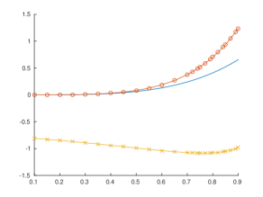
Figure 1: Caputo fractional derivatives of Example 2.1: $x(t)=t^{4}$ in continuous line, left derivative ${{}^{C}_{a}D_{t}^{\alpha(\cdot,\cdot)}}x(t)$ with “$\circ-$” style, and right derivative ${{}^{C}_{t}D_{b}^{\alpha(\cdot,\cdot)}}x(t)$ with “$\times-$” style.

Example 2.2.

In Example 2.1, we have used the polynomial $x(t)=t^{4}$. It is worth mentioning that our Chebfun implementation works well for functions that are not a polynomial. For example, let $x(t)=e^{t}$. In this case, we just need to change

  x = chebfun(@(t) t.^4, [a b]);

in Example 2.1 by

  x = chebfun(@(t) exp(t), [a b]);

to obtain

  LC(0.6)
  ans = 0.9917
  RC(0.6)
  ans = -1.1398

See Figure 2 for a plot with other values of ${{}^{C}_{a}D_{t}^{\alpha(\cdot,\cdot)}}x(t)$ and ${{}^{C}_{t}D_{b}^{\alpha(\cdot,\cdot)}}x(t)$.

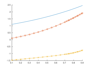
Figure 2: Caputo fractional derivatives of Example 2.2: $x(t)=e^{t}$ in continuous line, left derivative ${{}^{C}_{a}D_{t}^{\alpha(\cdot,\cdot)}}x(t)$ with “$\circ-$” style, and right derivative ${{}^{C}_{t}D_{b}^{\alpha(\cdot,\cdot)}}x(t)$ with “$\times-$” style.

Now, we define the generalized fractional integrals for variable order.

Definition 3 (Riemann–Liouville fractional integrals).

The left and right Riemann–Liouville fractional integrals of order ${\alpha_{n}(\cdot,\cdot)}$ are defined respectively by

$${{}_{a}I_{t}^{{\alpha_{n}(\cdot,\cdot)}}}x(t)=\int_{a}^{t}\frac{1}{\Gamma(\alpha_{n}(t,\tau))}(t-\tau)^{\alpha_{n}(t,\tau)-1}x(\tau)d\tau$$

and

$${{}_{t}I_{b}^{{\alpha_{n}(\cdot,\cdot)}}}x(t)=\int_{t}^{b}\frac{1}{\Gamma(\alpha_{n}(\tau,t))}(\tau-t)^{\alpha_{n}(\tau,t)-1}x(\tau)d\tau.$$

Our Chebfun definitions of the Riemann–Liouville fractional integrals are given in Appendix A.2. Here we illustrate their use.

Example 2.3.

Let $\alpha(t,\tau)=\frac{t^{2}+\tau^{2}}{4}$ and $x(t)=t^{2}$ with $t\in[0,1]$. In this case, $a=0$, $b=1$ and $n=1$. We have ${{}_{a}I_{0.6}^{\alpha(\cdot,\cdot)}}x(0.6)\approx 0.2661$ and ${{}_{0.6}I_{b}^{\alpha(\cdot,\cdot)}}x(0.6)\approx 0.4619$, obtained in Matlab with our Chebfun functions as follows:

  a = 0; b = 1; n = 1;
  alpha = @(t,tau) (t.^2+tau.^2)/4;
  x = chebfun(@(t) t.^2, [0,1]);
  LFI = leftFI(x,alpha,a);
  RFI = rightFI(x,alpha,b);
  LFI(0.6)
  ans = 0.2661
  RFI(0.6)
  ans = 0.4619

Other values for ${{}_{a}I_{t}^{\alpha(\cdot,\cdot)}}x(t)$ and ${{}_{t}I_{b}^{\alpha(\cdot,\cdot)}}x(t)$ are plotted in Figure 3.

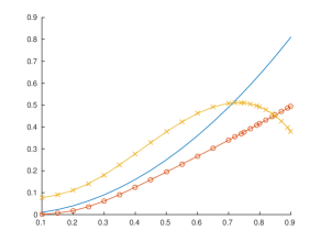
Figure 3: Riemann–Liouville fractional integrals of Example 2.3: $x(t)=t^{2}$ in continuous line, left integral ${{}_{a}I_{t}^{\alpha(\cdot,\cdot)}}x(t)$ with “$\circ-$” style, and right integral ${{}_{t}I_{b}^{\alpha(\cdot,\cdot)}}x(t)$ with “$\times-$” style.

Remark 2.

From Definition 3, it follows that

$${{}_{a}D_{t}^{{\alpha_{n}(\cdot,\cdot)}}}x(t)=\frac{d^{n}}{dt^{n}}\,_{a}I_{t}^{n-{\alpha_{n}(\cdot,\cdot)}}x(t),\quad{{}_{t}D_{b}^{{\alpha_{n}(\cdot,\cdot)}}}x(t)=(-1)^{n}\frac{d^{n}}{dt^{n}}\,_{t}I_{b}^{n-{\alpha_{n}(\cdot,\cdot)}}x(t)$$

and

$${{}^{C}_{a}D_{t}^{{\alpha_{n}(\cdot,\cdot)}}}x(t)=\,_{a}I_{t}^{n-{\alpha_{n}(\cdot,\cdot)}}\frac{d^{n}}{dt^{n}}x(t),\quad{{}^{C}_{t}D_{b}^{{\alpha_{n}(\cdot,\cdot)}}}x(t)=(-1)^{n}\,_{t}I_{b}^{n-{\alpha_{n}(\cdot,\cdot)}}\frac{d^{n}}{dt^{n}}x(t).$$

Next, we obtain higher-order Caputo fractional derivatives of a power function. This allows us to show the effectiveness of our computational approach, that is, the usefulness of polynomial interpolation in Chebyshev points in fractional calculus of variable order. In Lemma 2.4, we assume that the fractional order depends only on the first variable: $\alpha_{n}(t,\tau):=\overline{\alpha}_{n}(t)$, where $\overline{\alpha}_{n}:[a,b]\to(n-1,n)$ is a given function.

Lemma 2.4.

Let $x(t)=(t-a)^{\gamma}$ with $\gamma>n-1$. Then,

$${{}^{C}_{a}D_{t}^{\overline{\alpha}_{n}(t)}}x(t)=\frac{\Gamma(\gamma+1)}{\Gamma(\gamma-\overline{\alpha}_{n}(t)+1)}(t-a)^{\gamma-\overline{\alpha}_{n}(t)}.$$

Proof.

As $x(t)=(t-a)^{\gamma}$, if we differentiate it $n$ times, we obtain

$$x^{(n)}(t)=\frac{\Gamma(\gamma+1)}{\Gamma(\gamma-n+1)}(t-a)^{\gamma-n}.$$

Using Definition 2 of the left Caputo fractional derivative, we get

$$\begin{array}[]{ll}{{}^{C}_{a}D_{t}^{\overline{\alpha}_{n}(t)}}x(t)&=\displaystyle\int_{a}^{t}\frac{1}{\Gamma(n-\overline{\alpha}_{n}(t))}(t-\tau)^{n-1-\overline{\alpha}_{n}(t)}x^{(n)}(\tau)d\tau\\ &=\displaystyle\int_{a}^{t}\frac{\Gamma(\gamma+1)}{\Gamma(\gamma-n+1)\Gamma(n-\overline{\alpha}_{n}(t))}(t-\tau)^{n-1-\overline{\alpha}_{n}(t)}(\tau-a)^{\gamma-n}d\tau.\end{array}$$

Now, we proceed with the change of variables $\tau-a=s(t-a)$. Using the Beta function $B(\cdot,\cdot)$, we obtain that

$$\begin{array}[]{ll}{{}^{C}_{a}D_{t}^{\overline{\alpha}_{n}(t)}}x(t)&=\displaystyle\frac{\Gamma(\gamma+1)}{\Gamma(\gamma-n+1)\Gamma(n-\overline{\alpha}_{n}(t))}\int_{0}^{1}(1-s)^{n-1-\overline{\alpha}_{n}(t)}s^{\gamma-n}(t-a)^{\gamma-\overline{\alpha}_{n}(t)}ds\\ &=\displaystyle\frac{\Gamma(\gamma+1)(t-a)^{\gamma-\overline{\alpha}_{n}(t)}}{\Gamma(\gamma-n+1)\Gamma(n-\overline{\alpha}_{n}(t))}B\left(\gamma-n+1,n-\overline{\alpha}_{n}(t)\right).\\ &=\displaystyle\frac{\Gamma(\gamma+1)}{\Gamma(\gamma-\overline{\alpha}_{n}(t)+1)}\quad(t-a)^{\gamma-\overline{\alpha}_{n}(t)}.\end{array}$$

The proof is complete. ∎

Example 2.5.

Let us revisit Example 2.1 by choosing $\alpha(t,\tau)=\frac{t^{2}}{2}$ and $x(t)=t^{4}$ with $t\in[0,1]$. Table 1 shows the approximated values obtained by our Chebfun function leftCaputo(x,alpha,a,n) and the exact values computed with the formula given by Lemma 2.4. Table 1 was obtained using the following MATLAB code:

  format long
  a = 0; b = 1; n = 1;
  alpha = @(t,tau) t.^2/2;
  x = chebfun(@(t) t.^4, [a b]);
  exact = @(t) (gamma(5)./gamma(5-alpha(t))).*t.^(4-alpha(t));
  approximation = leftCaputo(x,alpha,a,n);
  for i = 1:9
    t = 0.1*i;
    E = exact(t);
    A = approximation(t);
    error = E - A;
    [t E A error]
  end

$\mathbf{t}$	Exact Value	Approximation	Error
0.1	1.019223177296953e-04	1.019223177296974e-04	-2.046431600566390e-18
0.2	0.001702793965464	0.001702793965464	-2.168404344971009e-18
0.3	0.009148530806348	0.009148530806348	3.469446951953614e-18
0.4	0.031052290994593	0.031052290994592	9.089951014118469e-16
0.5	0.082132144921157	0.082132144921157	6.522560269672795e-16
0.6	0.185651036003120	0.185651036003112	7.938094626069869e-15
0.7	0.376408251363662	0.376408251357416	6.246059225389899e-12
0.8	0.704111480975332	0.704111480816562	1.587694420379648e-10
0.9	1.236753486749357	1.236753486514274	2.350835082154390e-10

Table 1: Exact values obtained by Lemma 2.4 for functions of Example 2.5 versus computational approximations obtained using our Chebfun code of Appendix A.

For our next result, we assume that the fractional order depends only on the second variable: $\alpha_{n}(\tau,t):=\overline{\alpha}_{n}(t)$, where $\overline{\alpha}_{n}:[a,b]\to(n-1,n)$ is a given function. The proof is similar to that of Lemma 2.4, and so we omit it here.

Lemma 2.6.

Let $x(t)=(b-t)^{\gamma}$ with $\gamma>n-1$. Then,

$${{}^{C}_{t}D_{b}^{\overline{\alpha}_{n}(t)}}x(t)=\frac{\Gamma(\gamma+1)}{\Gamma(\gamma-\overline{\alpha}_{n}(t)+1)}(b-t)^{\gamma-\overline{\alpha}_{n}(t)}.$$

Computational experiments similar to those of Example 2.5, obtained by substituting Lemma 2.4 by Lemma 2.6 and our leftCaputo routine by the rightCaputo one, reinforce the validity of our computational methods.

When dealing with variational problems, one key property is integration by parts. In the following theorem, such formulas are proved for integrals involving higher-order Caputo fractional derivatives of variable order.

Theorem 2.7 (Integration by parts).

Let $n\in\mathbb{N}$ and $x,y\in C^{m}\left([a,b],\mathbb{R}\right)$ be two functions. Then,

$$\int_{a}^{b}y(t)\,{{}^{C}_{a}D_{t}^{{\alpha_{n}(\cdot,\cdot)}}}x(t)dt=\int_{a}^{b}x(t)\,{{{}_{t}D_{b}^{{\alpha_{n}(\cdot,\cdot)}}}}y(t)dt+\left[\sum_{k=0}^{n-1}(-1)^{k}x^{(n-1-k)}(t)\,\dfrac{d^{k}}{dt^{k}}{{}_{t}I_{b}^{n-{\alpha_{n}(\cdot,\cdot)}}}y(t)\right]_{a}^{b}$$

and

$$\int_{a}^{b}y(t)\,{{{}^{C}_{t}D_{b}^{{\alpha_{n}(\cdot,\cdot)}}}}x(t)dt=\int_{a}^{b}x(t)\,{{{}_{a}D_{t}^{{\alpha_{n}(\cdot,\cdot)}}}}y(t)dt+\left[\sum_{k=0}^{n-1}(-1)^{n+k}x^{(n-1-k)}(t)\,\dfrac{d^{k}}{dt^{k}}{{}_{a}I_{t}^{n-{\alpha_{n}(\cdot,\cdot)}}}y(t)\right]_{a}^{b}.$$

Proof.

Considering the definition of left Caputo fractional derivative of order ${\alpha_{n}(\cdot,\cdot)}$, we obtain

$$\int_{a}^{b}y(t)\,{{}^{C}_{a}D_{t}^{{\alpha_{n}(\cdot,\cdot)}}}x(t)dt=\int_{a}^{b}\int_{a}^{t}y(t)\,\dfrac{1}{\Gamma(n-\alpha_{n}(t,\tau))}(t-\tau)^{n-1-\alpha_{n}(t,\tau)}x^{(n)}(\tau)d\tau dt.$$

Using Dirichelet’s formula, we rewrite it as

$$\int_{a}^{b}\int_{t}^{b}y(\tau)\,\dfrac{(\tau-t)^{n-1-\alpha_{n}(\tau,t)}}{\Gamma(n-\alpha_{n}(\tau,t))}x^{(n)}(t)d\tau dt=\int_{a}^{b}x^{(n)}(t)\,{{}_{t}I_{b}^{n-{\alpha_{n}(\cdot,\cdot)}}}y(t)dt.$$ (3)

Using the (usual) integrating by parts formula, we get that (3) is equal to

$$-\int_{a}^{b}x^{(n-1)}(t)\dfrac{d}{dt}{{}_{t}I_{b}^{n-{\alpha_{n}(\cdot,\cdot)}}}y(t)dt+\left[x^{(n-1)}(t){{}_{t}I_{b}^{n-{\alpha_{n}(\cdot,\cdot)}}}y(t)\right]_{a}^{b}.$$

Integrating by parts again, we obtain

$$\begin{split}\int_{a}^{b}x^{(n-2)}(t)\,\dfrac{d^{2}}{dt^{2}}{{}_{t}I_{b}^{n-{\alpha_{n}(\cdot,\cdot)}}}y(t)dt+\left[x^{(n-1)}(t)\,{{}_{t}I_{b}^{n-{\alpha_{n}(\cdot,\cdot)}}}y(t)-x^{(n-2)}(t)\dfrac{d}{dt}{{}_{t}I_{b}^{n-{\alpha_{n}(\cdot,\cdot)}}}y(t)\right]_{a}^{b}.\end{split}$$

If we repeat this process $n-2$ times more, we get

$$\int_{a}^{b}x(t)(-1)^{n}\,\dfrac{d^{n}}{dt^{n}}{{}_{t}I_{b}^{n-{\alpha_{n}(\cdot,\cdot)}}}y(t)dt+\left[\sum_{k=0}^{n-1}(-1)^{k}x^{(n-1-k)}(t)\,\dfrac{d^{k}}{dt^{k}}{{}_{t}I_{b}^{n-{\alpha_{n}(\cdot,\cdot)}}}y(t)\right]_{a}^{b}\\ =\int_{a}^{b}x(t){{}_{t}D_{b}^{{\alpha_{n}(\cdot,\cdot)}}}y(t)dt+\left[\sum_{k=0}^{n-1}(-1)^{k}x^{(n-1-k)}(t)\,\dfrac{d^{k}}{dt^{k}}{{}_{t}I_{b}^{n-{\alpha_{n}(\cdot,\cdot)}}}y(t)\right]_{a}^{b}.$$

The second relation of the theorem for the right Caputo fractional derivative of order ${\alpha_{n}(\cdot,\cdot)}$ follows directly, from the first, by Caputo–Torres duality [9]. ∎

Remark 3.

If we consider in Theorem 2.7 the particular case when $n=1$, then the fractional integration by parts formulas take the following well-known forms

$$\int_{a}^{b}y(t)\,{{}^{C}_{a}D_{t}^{{\alpha(\cdot,\cdot)}}}x(t)dt=\int_{a}^{b}x(t)\,{{{}_{t}D_{b}^{{\alpha(\cdot,\cdot)}}}}y(t)dt+\left[x(t)\,{{}_{t}I_{b}^{1-{\alpha(\cdot,\cdot)}}}y(t)\right]_{a}^{b}$$

and

$$\int_{a}^{b}y(t)\,{{{}^{C}_{t}D_{b}^{{\alpha(\cdot,\cdot)}}}}x(t)dt=\int_{a}^{b}x(t)\,{{{}_{a}D_{t}^{{\alpha(\cdot,\cdot)}}}}y(t)dt-\left[x(t)\,{{}_{a}I_{t}^{1-{\alpha(\cdot,\cdot)}}}y(t)\right]_{a}^{b}$$

(see, e.g., [25, Theorem 3.2]).

Remark 4.

If $x$ is such that $x^{(i)}(a)=x^{(i)}(b)=0$ for all $i=0,\ldots,n-1$, then the higher-order formulas of fractional integration by parts given by Theorem 2.7 can be rewritten as

$$\int_{a}^{b}y(t)\,{{}^{C}_{a}D_{t}^{{\alpha_{n}(\cdot,\cdot)}}}x(t)dt=\int_{a}^{b}x(t)\,{{{}_{t}D_{b}^{{\alpha_{n}(\cdot,\cdot)}}}}y(t)dt,\quad\int_{a}^{b}y(t)\,{{{}^{C}_{t}D_{b}^{{\alpha_{n}(\cdot,\cdot)}}}}x(t)dt=\int_{a}^{b}x(t)\,{{{}_{a}D_{t}^{{\alpha_{n}(\cdot,\cdot)}}}}y(t)dt.$$

The next step is to consider a linear combination of the previous fractional derivatives.

Definition 4 (Higher-order combined fractional derivatives).

Let $\alpha_{n},\beta_{n}:[a,b]^{2}\rightarrow(n-1,n)$ be the variable fractional order, $\gamma^{n}=\left(\gamma_{1}^{n},\gamma_{2}^{n}\right)\in[0,1]^{2}$ a vector, and $x\in C^{n}\left([a,b]\right)$. The higher-order combined Riemann–Liouville fractional derivative of $x$ at $t$ is defined by

$$D_{\gamma^{n}}^{{\alpha_{n}(\cdot,\cdot)},{\beta_{n}(\cdot,\cdot)}}x(t)=\gamma_{1}^{n}\,{{}_{a}D_{t}^{{\alpha_{n}(\cdot,\cdot)}}}x(t)+\gamma_{2}^{n}\,{{}_{t}D_{b}^{{\beta_{n}(\cdot,\cdot)}}}x(t).$$

Analogously, the higher-order combined Caputo fractional derivative of $x$ at $t$ is defined by

$${}^{C}D_{\gamma^{n}}^{{\alpha_{n}(\cdot,\cdot)},{\beta_{n}(\cdot,\cdot)}}x(t)=\gamma_{1}^{n}\,{{}^{C}_{a}D_{t}^{{\alpha_{n}(\cdot,\cdot)}}}x(t)+\gamma_{2}^{n}\,{{}^{C}_{t}D_{b}^{{\beta_{n}(\cdot,\cdot)}}}x(t).$$

See our Chebfun computational code for the higher-order combined fractional Caputo derivative in Appendix A.3. Here we illustrate how to use it in MATLAB.

Example 2.8.

Let $\alpha(t,\tau)=\frac{t^{2}+\tau^{2}}{4}$, $\beta(t,\tau)=\frac{t+\tau}{3}$ and $x(t)=t$, $t\in[0,1]$. We have $a=0$, $b=1$ and $n=1$. For $\gamma=(\gamma_{1},\gamma_{2})=(0.8,0.2)$, we have ${}^{C}D_{\gamma}^{\alpha(\cdot,\cdot),\beta(\cdot,\cdot)}x(0.4)\approx 0.7144$:

  a = 0; b = 1; n = 1;
  alpha = @(t,tau) (t.^2 + tau.^2)/.4;
  beta = @(t,tau) (t + tau)/3;
  x = chebfun(@(t) t, [0 1]);
  gamma1 = 0.8;
  gamma2 = 0.2;
  CC = combinedCaputo(x,alpha,beta,gamma1,gamma2,a,b,n);
  CC(0.4)
  ans = 0.7144

3 Variational problems with higher-order derivatives

Given $n\in\mathbb{N}$, let $D$ denote the linear subspace of $C^{n}([a,b])\times[a,b]$ such that ${{}^{C}D_{\gamma^{i}}^{{\alpha_{i}(\cdot,\cdot)},{\beta_{i}(\cdot,\cdot)}}}x(t)$ exists and is continuous on the interval $[a,b]$ for all $i\in\{1,\ldots,n\}$. We endow $D$ with the norm

$$\|(x,t)\|=\max_{a\leq t\leq b}|x(t)|+\max_{a\leq t\leq b}\sum_{i=1}^{n}\left|{{}^{C}D_{\gamma^{i}}^{{\alpha_{i}(\cdot,\cdot)},{\beta_{i}(\cdot,\cdot)}}}x(t)\right|+|t|.$$

Consider the following problem of the calculus of variations: minimize functional $\mathcal{J}:D\rightarrow\mathbb{R}$,

$$\mathcal{J}(x,T)=\int_{a}^{T}L\left(t,x(t),\,^{C}D_{\gamma^{1}}^{\alpha_{1}(\cdot,\cdot),\beta_{1}(\cdot,\cdot)}x(t),\ldots,\,^{C}D_{\gamma^{n}}^{\alpha_{n}(\cdot,\cdot),\beta_{n}(\cdot,\cdot)}x(t)\right)dt+\phi(T,x(T)),$$ (4)

over all $(x,T)\in D$ subject to boundary conditions $x(a)=x_{a}$, $x^{(i)}(a)=x^{i}_{a}$, $\forall i\in\{1,\ldots,n-1\}$, for fixed $x_{a},x^{1}_{a},\ldots,x^{n-1}_{a}\in\mathbb{R}$. Here the terminal time $T$ and terminal state $x(T)$ are both free. For all $i\in\{1,\ldots,n\}$, $\alpha_{i},\beta_{i}\left([a,b]^{2}\right)\subseteq(i-1,i)$ and $\gamma^{i}=\left(\gamma_{1}^{i},\gamma_{2}^{i}\right)$ is a vector. The terminal cost function $\phi:[a,b]\times\mathbb{R}\rightarrow\mathbb{R}$ is at least of class $C^{1}$. For simplicity of notation, we introduce the operator $[\cdot]_{\gamma}^{\alpha,\beta}$ defined by $[x]_{\gamma}^{\alpha,\beta}(t)=\left(t,x(t),\,^{C}D_{\gamma^{1}}^{\alpha_{1}(\cdot,\cdot),\beta_{1}(\cdot,\cdot)}x(t),\ldots,\,^{C}D_{\gamma^{n}}^{\alpha_{n}(\cdot,\cdot),\beta_{n}(\cdot,\cdot)}x(t)\right)$. We assume that the Lagrangian $L:[a,b]\times\mathbb{R}^{n+1}\to\mathbb{R}$ is a function of class $C^{1}$. Along the work, we denote by $\partial_{i}L$, $i\in\{1,\ldots,n+2\}$, the partial derivative of the Lagrangian $L$ with respect to its $i$th argument.

Now, we can rewrite functional (4) as

$$\mathcal{J}(x,T)=\int_{a}^{T}L[x]_{\gamma}^{\alpha,\beta}(t)dt+\phi(T,x(T)).$$ (5)

In the sequel, we need the auxiliary notation of the dual fractional derivative:

$$D_{\overline{\gamma^{i}}}^{{\beta_{i}(\cdot,\cdot)},{\alpha_{i}(\cdot,\cdot)}}=\gamma_{2}^{i}\,{{}_{a}D_{t}^{{\beta_{i}(\cdot,\cdot)}}}+\gamma_{1}^{i}\,{{}_{t}D_{T}^{{\alpha_{i}(\cdot,\cdot)}}},\quad\mbox{where}\quad\overline{\gamma^{i}}=(\gamma_{2}^{i},\gamma_{1}^{i}).$$

In [34], we obtained fractional necessary optimality conditions that every local minimizer of functional $\mathcal{J}$, with $n=1$, must fulfill. Here, we generalize [34] to arbitrary values of $n$, $n\in\mathbb{N}$.

Theorem 3.1 (Necessary optimality conditions for (4)).

Suppose that $(x,T)$ gives a minimum to functional (5) on $D$. Then, $(x,T)$ satisfies the following fractional Euler–Lagrange equations:

$$\partial_{2}L[x]_{\gamma}^{\alpha,\beta}(t)+\sum_{i=1}^{n}{D_{\overline{\gamma^{i}}}^{{\beta_{i}(\cdot,\cdot)},{\alpha_{i}(\cdot,\cdot)}}}\partial_{i+2}L[x]_{\gamma}^{\alpha,\beta}(t)=0,$$ (6)

on the interval $[a,T]$, and

$$\sum_{i=1}^{n}\gamma_{2}^{i}\left({{}_{a}D_{t}^{{\beta_{i}(\cdot,\cdot)}}}\partial_{i+2}L[x]_{\gamma}^{\alpha,\beta}(t)-{{}_{T}D{{}_{t}^{{\beta_{i}(\cdot,\cdot)}}}\partial_{i+2}L[x]_{\gamma}^{\alpha,\beta}(t)}\right)=0,$$ (7)

on the interval $[T,b]$. Moreover, $(x,T)$ satisfies the following transversality conditions:

$$\begin{cases}L[x]_{\gamma}^{\alpha,\displaystyle\beta}(T)+\partial_{1}\phi(T,x(T))+\partial_{2}\phi(T,x(T))x^{\prime}(T)=0,\\ \displaystyle\sum_{i=1}^{n}\left[\gamma_{1}^{i}(-1)^{i-1}\,\frac{d^{i-1}}{dt^{i-1}}{{}_{t}I_{T}^{i-{\alpha_{i}(\cdot,\cdot)}}}\partial_{i+2}L[x]_{\gamma}^{\alpha,\beta}(t)\right.\\ \quad\quad\displaystyle-\left.\gamma_{2}^{i}\,\frac{d^{i-1}}{dt^{i-1}}{{}_{T}I_{t}^{i-{\beta_{i}(\cdot,\cdot)}}}\partial_{i+2}L[x]_{\gamma}^{\alpha,\beta}(t)\right]_{t=T}+\partial_{2}\phi(T,x(T))=0,\\ \displaystyle\sum_{i=j+1}^{n}\left[\gamma_{1}^{i}(-1)^{i-1-j}\,\frac{d^{i-1-j}}{dt^{i-1-j}}{{}_{t}I_{T}^{i-{\alpha_{i}(\cdot,\cdot)}}}\partial_{i+2}L[x]_{\gamma}^{\alpha,\beta}(t)\right.\\ \quad\quad\displaystyle+\left.\gamma_{2}^{i}(-1)^{j+1}\,\frac{d^{i-1-j}}{dt^{i-1-j}}{{}_{T}I_{t}^{i-{\beta_{i}(\cdot,\cdot)}}}\partial_{i+2}L[x]_{\gamma}^{\alpha,\beta}(t)\right]_{t=T}=0,\quad\forall j=1,\ldots,n-1,\\ \displaystyle\sum_{i=j+1}^{n}\left[\gamma_{2}^{i}(-1)^{j+1}\,\left[\frac{d^{i-1-j}}{dt^{i-1-j}}{{}_{a}I_{t}^{i-{\beta_{i}(\cdot,\cdot)}}}\partial_{i+2}L[x]_{\gamma}^{\alpha,\beta}(t)\right.\right.\\ \quad\quad\displaystyle\left.\left.-\,\frac{d^{i-1-j}}{dt^{i-1-j}}{{}_{T}I_{t}^{i-{\beta_{i}(\cdot,\cdot)}}\partial_{i+2}L[x]_{\gamma}^{\alpha,\beta}(t)}\right]\right]_{t=b}=0,\quad\forall j=0,\ldots,n-1.\end{cases}$$ (8)

Proof.

The proof is an extension of the one found in [34]. Let $h\in C^{n}([a,b])$ be a perturbing curve and $\triangle T\in\mathbb{R}$ an arbitrarily chosen small change in $T$. For a small number $\epsilon\in\mathbb{R}\left(\epsilon\rightarrow 0\right)$, if $(x,T)$ is a solution to the problem, we consider an admissible variation of $(x,T)$ of the form $\left(x+\epsilon{h},T+\epsilon\Delta{T}\right)$, and then, by the minimum condition, we have that $\mathcal{J}(x,T)\leq\mathcal{J}(x+\epsilon{h},T+\epsilon\Delta{T})$. The constraints $x^{(i)}(a)=x^{(i)}_{a}$ imply that all admissible variations must fulfill the conditions $h^{(i)}(a)=0,$ for all $i=0,\ldots,n-1$. We define function $j(\cdot)$ on a neighborhood of zero by

$$j(\epsilon)=\mathcal{J}(x+\epsilon h,T+\epsilon\triangle T)=\int_{a}^{T+\epsilon\triangle T}L[x+\epsilon h]_{\gamma}^{\alpha,\beta}(t)\,dt+\phi\left(T+\epsilon\triangle T,(x+\epsilon h)(T+\epsilon\triangle T)\right).$$

The derivative $j^{\prime}(\epsilon)$ is

$$\begin{split}j^{\prime}(\epsilon)&=\int_{a}^{T+\epsilon\triangle T}\left(\partial_{2}L[x+\epsilon h]_{\gamma}^{\alpha,\beta}(t)h(t)+\sum_{i=1}^{n}\partial_{i+2}L[x+\epsilon h]_{\gamma}^{\alpha,\beta}(t){{}^{C}D_{\gamma^{i}}^{{\alpha_{i}(\cdot,\cdot)},{\beta_{i}(\cdot,\cdot)}}}h(t)\right)dt\\ &\quad\quad+L[x+{\epsilon h}]_{\gamma}^{\alpha,\beta}(T+\epsilon\Delta T)\Delta T+\partial_{1}\phi\left(T+\epsilon\triangle T,(x+\epsilon h)(T+\epsilon\triangle T)\right)\,\Delta T\\ &\quad\quad+\partial_{2}\phi\left(T+\epsilon\triangle T,(x+\epsilon h)(T+\epsilon\triangle T)\right)\,(x+\epsilon h)^{\prime}(T+\epsilon\triangle T).\end{split}$$

Hence, a necessary condition for $(x,T)$ to be a local minimizer of $j$ is given by $j^{\prime}(0)=0$, that is,

$$\int_{a}^{T}\left(\partial_{2}L[x]_{\gamma}^{\alpha,\beta}(t)h(t)+\sum_{i=1}^{n}\partial_{i+2}L[x]_{\gamma}^{\alpha,\beta}(t){{}^{C}D_{\gamma^{i}}^{{\alpha_{i}(\cdot,\cdot)},{\beta_{i}(\cdot,\cdot)}}}h(t)\right)dt+L[x]_{\gamma}^{\alpha,\beta}(T)\Delta T\\ +\partial_{1}\phi\left(T,x(T)\right)\Delta T+\partial_{2}\phi(T,x(T))\left[h(t)+x^{\prime}(T)\triangle T\right]=0.$$ (9)

Considering the second addend of the integral function (9), for $i=1$, we get

$$\begin{split}&\int_{a}^{T}\partial_{3}L[x]_{\gamma}^{\alpha,\beta}(t){{}^{C}D_{\gamma^{1}}^{{\alpha_{1}(\cdot,\cdot)},{\beta_{1}(\cdot,\cdot)}}}h(t)dt=\int_{a}^{T}\partial_{3}L[x]_{\gamma}^{\alpha,\beta}(t)\left[\gamma_{1}^{1}\,{{}^{C}_{a}D_{t}^{{\alpha_{1}(\cdot,\cdot)}}}h(t)+\gamma_{2}^{1}\,{{}^{C}_{t}D_{b}^{{\beta_{1}(\cdot,\cdot)}}}h(t)\right]dt\\ &=\gamma_{1}^{1}\int_{a}^{T}\partial_{3}L[x]_{\gamma}^{\alpha,\beta}(t){{}^{C}_{a}D_{t}^{{\alpha_{1}(\cdot,\cdot)}}}h(t)dt\\ &\quad+\gamma_{2}^{1}\left[\int_{a}^{b}\partial_{3}L[x]_{\gamma}^{\alpha,\beta}(t){{}^{C}_{t}D_{b}^{{\beta_{1}(\cdot,\cdot)}}}h(t)dt-\int_{T}^{b}\partial_{3}L[x]_{\gamma}^{\alpha,\beta}(t){{}^{C}_{t}D_{b}^{{\beta_{1}(\cdot,\cdot)}}}h(t)dt\right].\end{split}$$

Integrating by parts (see Theorem 2.7), and since $h(a)=0$, we obtain that

$$\begin{split}\gamma_{1}^{1}&\left[\int_{a}^{T}h(t)_{t}D_{T}^{{\alpha_{1}(\cdot,\cdot)}}\partial_{3}L[x]_{\gamma}^{\alpha,\beta}(t)dt+\left[h(t){{}_{t}I_{T}^{1-{\alpha_{1}(\cdot,\cdot)}}\partial_{3}L[x]_{\gamma}^{\alpha,\beta}(t)}\right]_{t=T}\right]\\ &+\gamma_{2}^{1}\Biggl{[}\int_{a}^{b}h(t){{}_{a}D_{t}^{{\beta_{1}(\cdot,\cdot)}}}\partial_{3}L[x]_{\gamma}^{\alpha,\beta}(t)dt-\left[h(t){{}_{a}I_{t}^{1-{\beta_{1}(\cdot,\cdot)}}\partial_{3}L[x]_{\gamma}^{\alpha,\beta}(t)}\right]_{t=b}\\ &\qquad\quad-\Biggl{(}\int_{T}^{b}h(t){{}_{T}D_{t}^{{\beta_{1}(\cdot,\cdot)}}}\partial_{3}L[x]_{\gamma}^{\alpha,\beta}(t)dt-\left[h(t){{}_{T}I_{t}^{1-{\beta_{1}(\cdot,\cdot)}}\partial_{3}L[x]_{\gamma}^{\alpha,\beta}(t)}\right]_{t=b}\\ &\qquad\qquad\quad+\left[h(t){{}_{T}I_{t}^{1-{\beta_{1}(\cdot,\cdot)}}\partial_{3}L[x]_{\gamma}^{\alpha,\beta}(t)}\right]_{t=T}\Biggr{)}\Biggr{]}.\end{split}$$

Unfolding these integrals, and considering the fractional operator $D_{\overline{\gamma^{1}}}^{\beta_{1},\alpha_{1}}$ with $\overline{\gamma^{1}}=(\gamma_{2}^{1},\gamma_{1}^{1})$, then the previous term is equal to

$$\begin{split}\int_{a}^{T}h(t)&D_{\overline{\gamma^{1}}}^{{\beta_{1}(\cdot,\cdot)},{\alpha_{1}(\cdot,\cdot)}}\partial_{3}L[x]_{\gamma}^{\alpha,\beta}(t)dt\\ &+\int_{T}^{b}\gamma_{2}^{1}h(t)\left[{}_{a}D_{t}^{{\beta_{1}(\cdot,\cdot)}}\partial_{3}L[x]_{\gamma}^{\alpha,\beta}(t)-{{}_{T}D_{t}^{{\beta_{1}(\cdot,\cdot)}}\partial_{3}L[x]_{\gamma}^{\alpha,\beta}(t)}\right]dt\\ &+h(T)\left[\gamma_{1}^{1}\,{{}_{t}I_{T}^{1-{\alpha_{1}(\cdot,\cdot)}}\partial_{3}L[x]_{\gamma}^{\alpha,\beta}(t)}-{\gamma_{2}^{1}\,{{}_{T}I_{t}^{1-{\beta_{1}(\cdot,\cdot)}}\partial_{3}L[x]_{\gamma}^{\alpha,\beta}(t)}}\right]_{t=T}\\ &-h(b)\gamma_{2}^{1}\left[{{}_{a}I_{t}^{1-{\beta_{1}(\cdot,\cdot)}}\partial_{3}L[x]_{\gamma}^{\alpha,\beta}(t)}-{{}_{T}I_{t}^{1-{\beta_{1}(\cdot,\cdot)}}\partial_{3}L[x]_{\gamma}^{\alpha,\beta}(t)}\right]_{t=b}.\end{split}$$

Now, consider the general case $\displaystyle\int_{a}^{T}\partial_{i+2}L[x]_{\gamma}^{\alpha,\beta}(t){{}^{C}D_{\gamma^{i}}^{{\alpha_{i}(\cdot,\cdot)},{\beta_{i}(\cdot,\cdot)}}}h(t)dt$, $i=3,\ldots,n$. Then,

$$\begin{split}&\gamma_{1}^{i}\left[\int_{a}^{T}h(t)_{t}D_{T}^{{\alpha_{i}(\cdot,\cdot)}}\partial_{i+2}L[x]_{\gamma}^{\alpha,\beta}(t)dt+\left.\sum_{k=0}^{i-1}(-1)^{k}h^{(i-1-k)}(t)\frac{d^{k}}{dt^{k}}{{}_{t}I_{T}^{i-{\alpha_{i}(\cdot,\cdot)}}\partial_{i+2}L[x]_{\gamma}^{\alpha,\beta}(t)t)}\right]_{t=T}\right]\\ &+\gamma_{2}^{i}\Biggl{[}\int_{a}^{b}h(t){{}_{a}D_{t}^{{\beta_{i}(\cdot,\cdot)}}}\partial_{i+2}L[x]_{\gamma}^{\alpha,\beta}(t)dt+\left.\left.\sum_{k=0}^{i-1}(-1)^{i+k}h^{(i-1-k)}(t)\frac{d^{k}}{dt^{k}}{{}_{a}I_{t}^{i-{\beta_{i}(\cdot,\cdot)}}\partial_{i+2}L[x]_{\gamma}^{\alpha,\beta}(t)}\right]_{t=b}\right]\\ &-\gamma_{2}^{i}\left[\int_{T}^{b}h(t){{}_{T}D_{t}^{{\beta_{i}(\cdot,\cdot)}}}\partial_{i+2}L[x]_{\gamma}^{\alpha,\beta}(t)dt\right.+\left.\left.\sum_{k=0}^{i-1}(-1)^{i+k}h^{(i-1-k)}(t)\frac{d^{k}}{dt^{k}}{{}_{T}I_{t}^{i-{\beta_{i}(\cdot,\cdot)}}\partial_{i+2}L[x]_{\gamma}^{\alpha,\beta}(t)}\right]^{t=b}_{t=T}\right].\end{split}$$

Unfolding these integrals, we obtain

$$\begin{split}&\int_{a}^{T}h(t)D_{\overline{\gamma^{i}}}^{{\beta_{i}(\cdot,\cdot)},{\alpha_{i}(\cdot,\cdot)}}\partial_{i+2}L[x]_{\gamma}^{\alpha,\beta}(t)dt\\ &+\int_{T}^{b}\gamma_{2}^{i}h(t)\left[{}_{a}D_{t}^{{\beta_{i}(\cdot,\cdot)}}\partial_{i+2}L[x]_{\gamma}^{\alpha,\beta}(t)-{{}_{T}D_{t}^{{\beta_{i}(\cdot,\cdot)}}\partial_{i+2}L[x]_{\gamma}^{\alpha,\beta}(t)}\right]dt\\ &+h^{(i-1)}(T)\left[\gamma_{1}^{i}\,{{}_{t}I_{T}^{i-{\alpha_{i}(\cdot,\cdot)}}\partial_{i+2}L[x]_{\gamma}^{\alpha,\beta}(t)}+{\gamma_{2}^{i}(-1)^{i}\,{{}_{T}I_{t}^{i-{\beta_{i}(\cdot,\cdot)}}\partial_{i+2}L[x]_{\gamma}^{\alpha,\beta}(t)}}\right]_{t=T}\\ &+h^{(i-1)}(b)\gamma_{2}^{i}(-1)^{i}\left[\,{{}_{a}I_{t}^{i-{\beta_{i}(\cdot,\cdot)}}\partial_{i+2}L[x]_{\gamma}^{\alpha,\beta}(t)}-{{}_{T}I_{t}^{i-{\beta_{i}(\cdot,\cdot)}}\partial_{i+2}L[x]_{\gamma}^{\alpha,\beta}(t)}\right]_{t=b}\\ &+h^{(i-2)}(T)\left[\gamma_{1}^{i}(-1)^{1}\frac{d}{dt}\,{{}_{t}I_{T}^{i-{\alpha_{i}(\cdot,\cdot)}}\partial_{i+2}L[x]_{\gamma}^{\alpha,\beta}(t)}+{\gamma_{2}^{i}(-1)^{i+1}\frac{d}{dt}\,{{}_{T}I_{t}^{i-{\beta_{i}(\cdot,\cdot)}}\partial_{i+2}L[x]_{\gamma}^{\alpha,\beta}(t)}}\right]_{t=T}\\ &+h^{(i-2)}(b)\gamma_{2}^{i}(-1)^{i+1}\left[\,\frac{d}{dt}{{}_{a}I_{t}^{i-{\beta_{i}(\cdot,\cdot)}}\partial_{i+2}L[x]_{\gamma}^{\alpha,\beta}(t)}-\frac{d}{dt}{{}_{T}I_{t}^{i-{\beta_{i}(\cdot,\cdot)}}\partial_{i+2}L[x]_{\gamma}^{\alpha,\beta}(t)}\right]_{t=b}\\ &\qquad\vdots\\ &+h(T)\left[\gamma_{1}^{i}(-1)^{i-1}\frac{d^{i-1}}{dt^{i-1}}{{}_{t}I_{T}^{i-{\alpha_{i}(\cdot,\cdot)}}\partial_{i+2}L[x]_{\gamma}^{\alpha,\beta}(t)}+\gamma_{2}^{i}(-1)^{2i-1}\frac{d^{i-1}}{dt^{i-1}}{{}_{T}I_{t}^{i-{\beta_{i}(\cdot,\cdot)}}\partial_{i+2}L[x]_{\gamma}^{\alpha,\beta}(t)}\right]_{t=T}\\ &+h(b)\gamma_{2}^{i}(-1)^{2i-1}\left[\frac{d^{i-1}}{dt^{i-1}}{{}_{a}I_{t}^{i-{\beta_{i}(\cdot,\cdot)}}\partial_{i+2}L[x]_{\gamma}^{\alpha,\beta}(t)}-\frac{d^{i-1}}{dt^{i-1}}{{}_{T}I_{t}^{i-{\beta_{i}(\cdot,\cdot)}}\partial_{i+2}L[x]_{\gamma}^{\alpha,\beta}(t)}\right]_{t=b}.\end{split}$$

Substituting all the relations into equation (9), we obtain that

$$\begin{split}0=&\int_{a}^{T}h(t)\left(\partial_{2}L[x]_{\gamma}^{\alpha,\beta}(t)+\sum_{i=1}^{n}D_{\overline{\gamma^{i}}}^{{\beta_{i}(\cdot,\cdot)},{\alpha_{i}(\cdot,\cdot)}}\partial_{i+2}L[x]_{\gamma}^{\alpha,\beta}(t)\right)dt\\ &+\int_{T}^{b}h(t)\sum_{i=1}^{n}\gamma_{2}^{i}\left[{}_{a}D_{t}^{{\beta_{i}(\cdot,\cdot)}}\partial_{i+2}L[x]_{\gamma}^{\alpha,\beta}(t)-{{}_{T}D_{t}^{{\beta_{i}(\cdot,\cdot)}}\partial_{i+2}L[x]_{\gamma}^{\alpha,\beta}(t)}\right]dt\\ &+\sum_{j=0}^{n-1}h^{(j)}(T)\sum_{i=j+1}^{n}\left[\gamma_{1}^{i}(-1)^{i-1-j}\frac{d^{i-1-j}}{dt^{i-1-j}}{{}_{t}I_{T}^{i-{\alpha_{i}(\cdot,\cdot)}}\partial_{i+2}L[x]_{\gamma}^{\alpha,\beta}(t)}\right.\\ &\quad\quad\quad\quad\quad\quad\quad\quad\left.+\gamma_{2}^{i}(-1)^{j+1}\frac{d^{i-1-j}}{dt^{i-1-j}}{{}_{T}I_{t}^{i-{\beta_{i}(\cdot,\cdot)}}\partial_{i+2}L[x]_{\gamma}^{\alpha,\beta}(t)}\right]_{t=T}\\ &+\sum_{j=0}^{n-1}h^{(j)}(b)\sum_{i=j+1}^{n}\gamma_{2}^{i}(-1)^{j+1}\left[\frac{d^{i-1-j}}{dt^{i-1-j}}{{}_{a}I_{t}^{i-{\beta_{i}(\cdot,\cdot)}}\partial_{i+2}L[x]_{\gamma}^{\alpha,\beta}(t)}\right.\\ &\quad\quad\quad\quad\quad\quad\quad\quad\left.-\frac{d^{i-1-j}}{dt^{i-1-j}}{{}_{T}I_{t}^{i-{\beta_{i}(\cdot,\cdot)}}\partial_{i+2}L[x]_{\gamma}^{\alpha,\beta}(t)}\right]_{t=b}\\ &+h(T)\partial_{2}\phi\left(T,x(T)\right)+\Delta T\left[L[x]_{\gamma}^{\alpha,\beta}(T)+\partial_{1}\phi\left(T,x(T)\right)+\partial_{2}\phi(T,x(T))x^{\prime}(T)\right].\end{split}$$ (10)

The fractional Euler–Lagrange equations (6)–(7) and the transversality conditions (8) follow by application of the fundamental lemma of the calculus of variations (see, e.g., [39]), for appropriate choices of variations. ∎

4 Variational problems with time delay

In this section, we consider fractional variational problems with time delay. As mentioned in [37], “We verify that a fractional derivative requires an infinite number of samples capturing, therefore, all the signal history, contrary to what happens with integer order derivatives that are merely local operators. This fact motivates the evaluation of calculation strategies based on delayed signal samples”. This subject has already been studied for constant fractional order [3, 8, 13, 14]. However, for a variable fractional order, it is, to the authors’ best knowledge, an open question. We also refer to the works [10, 11, 16, 40], where fractional differential equations are considered with a time delay. For simplicity of presentation, we consider fractional orders $\alpha,\beta:[a,b]^{2}\to(0,1)$. Using similar arguments, the problem can be easily generalized for higher-order derivatives. Let $\sigma>0$ and define the vector ${}_{\sigma}[x]_{\gamma}^{\alpha,\beta}(t)=\left(t,x(t),{{}^{C}D_{\gamma}^{{\alpha(\cdot,\cdot)},{\beta(\cdot,\cdot)}}}x(t),x(t-\sigma)\right)$. For the domain of the functional, we consider the set

$$D_{\sigma}=\left\{(x,t)\in C^{1}([a-\sigma,b])\times[a,b]:\quad{{}^{C}D_{\gamma}^{{\alpha(\cdot,\cdot)},{\beta(\cdot,\cdot)}}}x(t)\,\mbox{ exists and is continuous on }[a,b]\right\}.$$

Let $\mathcal{J}:D\to\mathbb{R}$ be the functional defined by

$$\mathcal{J}(x,T)=\int_{a}^{T}L_{\sigma}[x]_{\gamma}^{\alpha,\beta}(t)+\phi(T,x(T))$$ (11)

subject to the boundary condition $x(t)=\varphi(t)$ for all $t\in[a-\sigma,a]$, where $\varphi$ is a given (fixed) function. Again, we assume that the Lagrangian $L$ and the payoff term $\phi$ are differentiable functions and we denote, for $T\in[a,b]$, $D_{\overline{\gamma}}^{{\beta(\cdot,\cdot)},{\alpha(\cdot,\cdot)}}=\gamma_{2}$, ${{}_{a}D_{t}^{{\beta(\cdot,\cdot)}}}+\gamma_{1}\,{{}_{t}D_{T}^{{\alpha(\cdot,\cdot)}}}$, where $\overline{\gamma}=(\gamma_{2},\gamma_{1})$.

Theorem 4.1 (Necessary optimality conditions for (11)).

Suppose that $(x,T)$ gives a local minimum to functional (11) on $D_{\sigma}$. If $\sigma\geq T-a$, then $(x,T)$ satisfies

$$\partial_{2}L_{\sigma}[x]_{\gamma}^{\alpha,\beta}(t)+D{{}_{\overline{\gamma}}^{{\beta(\cdot,\cdot)},{\alpha(\cdot,\cdot)}}}\partial_{3}L_{\sigma}[x]_{\gamma}^{\alpha,\beta}(t)=0,$$ (12)

for $t\in[a,T]$, and

$$\gamma_{2}\left({{{}_{a}D_{t}^{{\beta(\cdot,\cdot)}}}}\partial_{3}L_{\sigma}[x]_{\gamma}^{\alpha,\beta}(t)-{{}_{T}D{{}_{t}^{{\beta(\cdot,\cdot)}}}\partial_{3}L_{\sigma}[x]_{\gamma}^{\alpha,\beta}(t)}\right)=0,$$ (13)

for $t\in[T,b]$. Moreover, $(x,T)$ satisfies

$$\begin{cases}L_{\sigma}[x]_{\gamma}^{\alpha,\beta}(T)+\partial_{1}\phi(T,x(T))+\partial_{2}\phi(T,x(T))x^{\prime}(T)=0,\\ \left[\gamma_{1}\,{{}_{t}I_{T}^{1-{\alpha(\cdot,\cdot)}}}\partial_{3}L_{\sigma}[x]_{\gamma}^{\alpha,\beta}(t)-\gamma_{2}\,{{}_{T}I_{t}^{1-{\beta(\cdot,\cdot)}}}\partial_{3}L_{\sigma}[x]_{\gamma}^{\alpha,\beta}(t)\right]_{t=T}+\partial_{2}\phi(T,x(T))=0,\\ \gamma_{2}\left[{{}_{T}I_{t}^{1-{\beta(\cdot,\cdot)}}}\partial_{3}L_{\sigma}[x]_{\gamma}^{\alpha,\beta}(t)-{{}_{a}I_{t}^{1-{\beta(\cdot,\cdot)}}\partial_{3}L_{\sigma}[x]_{\gamma}^{\alpha,\beta}(t)}\right]_{t=b}=0.\end{cases}$$ (14)

If $\sigma<T-a$, then Eq. (12) is replaced by the two following ones:

$$\partial_{2}L_{\sigma}[x]_{\gamma}^{\alpha,\beta}(t)+D{{}_{\overline{\gamma}}^{{\beta(\cdot,\cdot)},{\alpha(\cdot,\cdot)}}}\partial_{3}L_{\sigma}[x]_{\gamma}^{\alpha,\beta}(t)+\partial_{4}L_{\sigma}[x]_{\gamma}^{\alpha,\beta}(t+\sigma)=0,$$ (15)

for $t\in[a,T-\sigma]$, and

$$\partial_{2}L_{\sigma}[x]_{\gamma}^{\alpha,\beta}(t)+D{{}_{\overline{\gamma}}^{{\beta(\cdot,\cdot)},{\alpha(\cdot,\cdot)}}}\partial_{3}L_{\sigma}[x]_{\gamma}^{\alpha,\beta}(t)=0,$$ (16)

for $t\in[T-\sigma,T]$.

Proof.

Consider variations of the solution $\left(x+\epsilon h,T+\epsilon\Delta{T}\right)$, where $h\in C^{1}([a-\sigma,b])$ is such that $h(t)=0$ for all $t\in[a-\sigma,a]$, and $\epsilon,\triangle T$ are two reals. If we define $j(\epsilon)=\mathcal{J}\left(x+\epsilon h,T+\epsilon\Delta{T}\right)$, then $j^{\prime}(0)=0$, that is,

$$\int_{a}^{T}\left(\partial_{2}L_{\sigma}[x]_{\gamma}^{\alpha,\beta}(t)h(t)+\partial_{3}L_{\sigma}[x]_{\gamma}^{\alpha,\beta}(t){{}^{C}D_{\gamma}^{{\alpha(\cdot,\cdot)},{\beta(\cdot,\cdot)}}}h(t)+\partial_{4}L_{\sigma}[x]_{\gamma}^{\alpha,\beta}(t)h(t-\sigma)\right)dt\\ +L_{\sigma}[x]_{\gamma}^{\alpha,\beta}(T)\Delta T+\partial_{1}\phi\left(T,x(T)\right)\Delta T+\partial_{2}\phi(T,x(T))\left[h(T)+x^{\prime}(T)\triangle T\right]=0.$$ (17)

First, suppose that $\sigma\geq T-a$. In this case, since

$$\int_{a}^{T}\partial_{4}L_{\sigma}[x]_{\gamma}^{\alpha,\beta}(t)h(t-\sigma)\,dt=\int_{a-\sigma}^{T-\sigma}\partial_{4}L_{\sigma}[x]_{\gamma}^{\alpha,\beta}(t+\sigma)h(t)\,dt$$

and $h\equiv 0$ on $[a-\sigma,a]$, this term vanishes in (17) and we obtain Eq. (5) of [34]. The rest of the proof is similar to the one presented in [34, Theorem 3.1], and we obtain (12)–(14). Suppose now that $\sigma<T-a$. In this case, we have that

$$\int_{a}^{T}\partial_{4}L_{\sigma}[x]_{\gamma}^{\alpha,\beta}(t)h(t-\sigma)\,dt=\int_{a-\sigma}^{T-\sigma}\partial_{4}L_{\sigma}[x]_{\gamma}^{\alpha,\beta}(t+\sigma)h(t)\,dt=\int_{a}^{T-\sigma}\partial_{4}L_{\sigma}[x]_{\gamma}^{\alpha,\beta}(t+\sigma)h(t)\,dt.$$

Next, we evaluate the integral

$$\int_{a}^{T}\partial_{3}L_{\sigma}[x]_{\gamma}^{\alpha,\beta}(t){{}^{C}D_{\gamma}^{{\alpha(\cdot,\cdot)},{\beta(\cdot,\cdot)}}}h(t)\,dt\\ =\int_{a}^{T-\sigma}\partial_{3}L_{\sigma}[x]_{\gamma}^{\alpha,\beta}(t){{}^{C}D_{\gamma}^{{\alpha(\cdot,\cdot)},{\beta(\cdot,\cdot)}}}h(t)\,dt+\int_{T-\sigma}^{T}\partial_{3}L_{\sigma}[x]_{\gamma}^{\alpha,\beta}(t){{}^{C}D_{\gamma}^{{\alpha(\cdot,\cdot)},{\beta(\cdot,\cdot)}}}h(t)\,dt.$$

For the first integral, integrating by parts, we have

$$\int_{a}^{T-\sigma}\partial_{3}L_{\sigma}[x]_{\gamma}^{\alpha,\beta}(t){{}^{C}D_{\gamma}^{{\alpha(\cdot,\cdot)},{\beta(\cdot,\cdot)}}}h(t)\,dt=\gamma_{1}\int_{a}^{T-\sigma}\partial_{3}L_{\sigma}[x]_{\gamma}^{\alpha,\beta}(t){{}^{C}_{a}D_{t}^{{\alpha(\cdot,\cdot)}}}h(t)dt$$

$$\quad+\gamma_{2}\left[\int_{a}^{b}\partial_{3}L_{\sigma}[x]_{\gamma}^{\alpha,\beta}(t){{}^{C}_{t}D_{b}^{{\beta(\cdot,\cdot)}}}h(t)dt-\int_{T-\sigma}^{b}\partial_{3}L_{\sigma}[x]_{\gamma}^{\alpha,\beta}(t){{}^{C}_{t}D_{b}^{{\beta(\cdot,\cdot)}}}h(t)dt\right]$$

$$=\int_{a}^{T-\sigma}h(t)\left[{\gamma_{1}}{{}_{t}D_{T-\sigma}^{{\alpha(\cdot,\cdot)}}}\partial_{3}L_{\sigma}[x]_{\gamma}^{\alpha,\beta}(t)+{\gamma_{2}}{{}_{a}D_{t}^{{\beta(\cdot,\cdot)}}}\partial_{3}L_{\sigma}[x]_{\gamma}^{\alpha,\beta}(t)\right]dt$$

$$\quad+\int_{T-\sigma}^{b}\gamma_{2}h(t)\left[{{}_{a}D_{t}^{{\beta(\cdot,\cdot)}}}\partial_{3}L_{\sigma}[x]_{\gamma}^{\alpha,\beta}(t)-{{}_{T-\sigma}D_{t}^{{\beta(\cdot,\cdot)}}}\partial_{3}L_{\sigma}[x]_{\gamma}^{\alpha,\beta}(t)\right]dt$$

$$\quad+\left[h(t)\left[{\gamma_{1}}{{}_{t}I_{T-\sigma}^{1-{\alpha(\cdot,\cdot)}}}\partial_{3}L_{\sigma}[x]_{\gamma}^{\alpha,\beta}(t)-{\gamma_{2}}{{}_{T-\sigma}I_{t}^{1-{\beta(\cdot,\cdot)}}}\partial_{3}L_{\sigma}[x]_{\gamma}^{\alpha,\beta}(t)\right]\right]_{t=T-\sigma}$$

$$\quad+\left[\gamma_{2}h(t)\left[-{{}_{a}I_{t}^{1-{\beta(\cdot,\cdot)}}}\partial_{3}L_{\sigma}[x]_{\gamma}^{\alpha,\beta}(t)+{{}_{T-\sigma}I_{t}^{1-{\beta(\cdot,\cdot)}}}\partial_{3}L_{\sigma}[x]_{\gamma}^{\alpha,\beta}(t)\right]\right]_{t=b}.$$

For the second integral, in a similar way, we deduce that

$$\int_{T-\sigma}^{T} \partial_{3}L_{\sigma}[x]_{\gamma}^{\alpha,\beta}(t){{}^{C}D_{\gamma}^{{\alpha(\cdot,\cdot)},{\beta(\cdot,\cdot)}}}h(t)\,dt$$

$$=\gamma_{1}\left[\int_{a}^{T}\partial_{3}L_{\sigma}[x]_{\gamma}^{\alpha,\beta}(t){{}^{C}_{a}D_{t}^{{\alpha(\cdot,\cdot)}}}h(t)dt-\int_{a}^{T-\sigma}\partial_{3}L_{\sigma}[x]_{\gamma}^{\alpha,\beta}(t){{}^{C}_{a}D_{t}^{{\alpha(\cdot,\cdot)}}}h(t)dt\right]$$

$$\quad+\gamma_{2}\left[\int_{T-\sigma}^{b}\partial_{3}L_{\sigma}[x]_{\gamma}^{\alpha,\beta}(t){{}^{C}_{t}D_{b}^{{\beta(\cdot,\cdot)}}}h(t)dt-\int_{T}^{b}\partial_{3}L_{\sigma}[x]_{\gamma}^{\alpha,\beta}(t){{}^{C}_{t}D_{b}^{{\beta(\cdot,\cdot)}}}h(t)dt\right]$$

$$=\int_{a}^{T-\sigma}\gamma_{1}h(t)\left[{{}_{t}D_{T}^{{\alpha(\cdot,\cdot)}}}\partial_{3}L_{\sigma}[x]_{\gamma}^{\alpha,\beta}(t)-{{}_{t}D_{T-\sigma}^{{\alpha(\cdot,\cdot)}}}\partial_{3}L_{\sigma}[x]_{\gamma}^{\alpha,\beta}(t)\right]dt$$

$$\quad+\int_{T-\sigma}^{T}h(t)\left[{\gamma_{1}}{{}_{t}D_{T}^{{\alpha(\cdot,\cdot)}}}\partial_{3}L_{\sigma}[x]_{\gamma}^{\alpha,\beta}(t)+{\gamma_{2}}{{}_{T-\sigma}D_{t}^{{\beta(\cdot,\cdot)}}}\partial_{3}L_{\sigma}[x]_{\gamma}^{\alpha,\beta}(t)\right]dt$$

$$\quad+\int_{T}^{b}\gamma_{2}h(t)\left[{{}_{T-\sigma}D_{t}^{{\beta(\cdot,\cdot)}}}\partial_{3}L_{\sigma}[x]_{\gamma}^{\alpha,\beta}(t)-{{}_{T}D_{t}^{{\beta(\cdot,\cdot)}}}\partial_{3}L_{\sigma}[x]_{\gamma}^{\alpha,\beta}(t)\right]dt$$

$$\quad+\left[h(t)\left[-{\gamma_{1}}{{}_{t}I_{T-\sigma}^{1-{\alpha(\cdot,\cdot)}}}\partial_{3}L_{\sigma}[x]_{\gamma}^{\alpha,\beta}(t)+{\gamma_{2}}{{}_{T-\sigma}I_{t}^{1-{\beta(\cdot,\cdot)}}}\partial_{3}L_{\sigma}[x]_{\gamma}^{\alpha,\beta}(t)\right]\right]_{t=T-\sigma}$$

$$\quad+\left[h(t)\left[{\gamma_{1}}{{}_{t}I_{T}^{1-{\alpha(\cdot,\cdot)}}}\partial_{3}L_{\sigma}[x]_{\gamma}^{\alpha,\beta}(t)-{\gamma_{2}}{{}_{T}I_{t}^{1-{\beta(\cdot,\cdot)}}}\partial_{3}L_{\sigma}[x]_{\gamma}^{\alpha,\beta}(t)\right]\right]_{t=T}$$

$$\quad+\left[\gamma_{2}h(t)\left[-{{}_{T-\sigma}I_{t}^{1-{\beta(\cdot,\cdot)}}}\partial_{3}L_{\sigma}[x]_{\gamma}^{\alpha,\beta}(t)+{{}_{T}I_{t}^{1-{\beta(\cdot,\cdot)}}}\partial_{3}L_{\sigma}[x]_{\gamma}^{\alpha,\beta}(t)\right]\right]_{t=b}.$$

Replacing the above equalities into (17), we prove that

$$0= \int_{a}^{T-\sigma}h(t)\left[\partial_{2}L_{\sigma}[x]_{\gamma}^{\alpha,\beta}(t)+D_{\overline{\gamma}}^{{\beta(\cdot,\cdot)},{\alpha(\cdot,\cdot)}}\partial_{3}L_{\sigma}[x]_{\gamma}^{\alpha,\beta}(t)+\partial_{4}L_{\sigma}[x]_{\gamma}^{\alpha,\beta}(t+\sigma)\right]dt$$

$$+\int_{T-\sigma}^{T}h(t)\left[\partial_{2}L_{\sigma}[x]_{\gamma}^{\alpha,\beta}(t)+D_{\overline{\gamma}}^{{\beta(\cdot,\cdot)},{\alpha(\cdot,\cdot)}}\partial_{3}L_{\sigma}[x]_{\gamma}^{\alpha,\beta}(t)\right]dt$$

$$+\int_{T}^{b}\gamma_{2}h(t)\left[{}_{a}D_{t}^{{\beta(\cdot,\cdot)}}\partial_{3}L_{\sigma}[x]_{\gamma}^{\alpha,\beta}(t)-{{}_{T}D_{t}^{{\beta(\cdot,\cdot)}}\partial_{3}L_{\sigma}[x]_{\gamma}^{\alpha,\beta}(t)}\right]dt$$

$$+h(T)\left[\gamma_{1}\,{{}_{t}I_{T}^{1-{\alpha(\cdot,\cdot)}}\partial_{3}L_{\sigma}[x]_{\gamma}^{\alpha,\beta}(t)}-{\gamma_{2}\,{{}_{T}I_{t}^{1-{\beta(\cdot,\cdot)}}\partial_{3}L_{\sigma}[x]_{\gamma}^{\alpha,\beta}(t)}}+\partial_{2}\phi(t,x(t))\right]_{t=T}$$

$$+\Delta T\left[L_{\sigma}[x]_{\gamma}^{\alpha,\beta}(t)+\partial_{1}\phi(t,x(t))+\partial_{2}\phi(t,x(t))x^{\prime}(t)\right]_{t=T}$$

$$+h(b)\left[\gamma_{2}\left({}_{T}I_{t}^{1-{\beta(\cdot,\cdot)}}\partial_{3}L_{\sigma}[x]_{\gamma}^{\alpha,\beta}(t)-{{}_{a}I_{t}^{1-{\beta(\cdot,\cdot)}}\partial_{3}L_{\sigma}[x]_{\gamma}^{\alpha,\beta}(t)}\right)\right]_{t=b}.$$

By the arbitrariness of $h$ in $[a,b]$ and of $\triangle T$, we obtain Eqs. (13)–(16). ∎

5 Examples

We provide two illustrative examples. Example 5.1 is covered by Theorem 3.1 while Example 5.2 illustrates Theorem 4.1.

Example 5.1.

Let $p_{n-1}(t)$ be a polynomial of degree $n-1$. If $\alpha,\beta:[0,b]^{2}\to(n-1,n)$ are the fractional orders, then ${{}^{C}D_{\gamma}^{{\alpha(\cdot,\cdot)},{\beta(\cdot,\cdot)}}}p_{n-1}(t)=0$ since $p_{n-1}^{(n)}(t)=0$ for all $t$. Consider

$$\mathcal{J}(x,T)=\int_{0}^{T}\left[\left({{}^{C}D_{\gamma}^{{\alpha(\cdot,\cdot)},{\beta(\cdot,\cdot)}}}x(t)\right)^{2}+(x(t)-p_{n-1}(t))^{2}-t-1\right]\,dt+T^{2}$$

subject to the initial constraints $x(0)=p_{n-1}(0)$ and $x^{(k)}(0)=p_{n-1}^{(k)}(0)$, $k=1,\ldots,n-1$. Observe that, for all $t\in[0,b]$, $\partial_{2}L[x]_{\gamma}^{\alpha,\beta}(t)=2(x(t)-p_{n-1}(t))$ and $\partial_{3}L[x]_{\gamma}^{\alpha,\beta}(t)=2\,{{}^{C}D_{\gamma}^{{\alpha(\cdot,\cdot)},{\beta(\cdot,\cdot)}}}x(t)$. Therefore, $\partial_{i}L[p_{n-1}]_{\gamma}^{\alpha,\beta}(t)=0$, $i=2,3$. Also, the first transversality condition reads as

$$\left({{}^{C}D_{\gamma}^{{\alpha(\cdot,\cdot)},{\beta(\cdot,\cdot)}}}x(T)\right)^{2}+(x(T)-p_{n-1}(T))^{2}-T-1+2T=0,$$

which is verified at $(x,T)=(p_{n-1},1)$. Thus, function $x\equiv p_{n-1}$ and the final time $T=1$ satisfy the necessary optimality conditions of Theorem 3.1. We also remark that one has

$$\mathcal{J}(x,T)\geq\int_{0}^{T}\left[-t-1\right]\,dt+T^{2}=\frac{T^{2}}{2}-T$$

for any curve $x$, which attains a minimum value $-1/2$ at $T=1$. Since $\mathcal{J}(p_{n-1},1)=-1/2$, we conclude that $(p_{n-1},1)$ is the (global) minimizer of $\mathcal{J}$.

Example 5.2.

Let $\alpha,\beta:[0,b]^{2}\to(0,1)$, $f$ be a function of class $C^{1}$, and $\hat{f}(t)={{}^{C}D_{\gamma}^{{\alpha(\cdot,\cdot)},{\beta(\cdot,\cdot)}}}f(t)$. Define $\mathcal{J}$ as

$$\mathcal{J}(x,T)=\int_{0}^{T}\Biggl{[}\left({{}^{C}D_{\gamma}^{{\alpha(\cdot,\cdot)},{\beta(\cdot,\cdot)}}}x(t)-\hat{f}(t)\right)^{2}+(x(t)-f(t))^{2}+(x(t-1)-f(t-1))^{2}-t-2\Biggr{]}\,dt+T^{2}$$

subject to the condition $x(t)=f(t)$ for all $t\in[-1,0]$. In this case, we can easily verify that $(x,T)=(f,2)$ satisfies all the conditions in Theorem 4.1, because $\partial_{i}L_{\sigma}[p_{n-1}]_{\gamma}^{\alpha,\beta}(t)=0$, $i=2,3,4$, and that it is actually the (global) minimizer of the problem.

6 Conclusion

We studied two different types of fractional variational problems of variable order: of higher-order and with a time delay. Necessary optimality conditions of Euler–Lagrange type for such functionals, containing a combined Caputo derivative of variable fractional order, were established. To solve such fractional differential equations, we presented a numerical method to deal with the fractional operators, based on the open source software package Chebfun. Examples were discussed in order to illustrate the new findings and the computational aspects of the work.

Appendix A Chebfun code

Chebfun is an open source software package that “aims to provide numerical computing with functions” in MATLAB [19]. For the mathematical underpinnings of Chebfun, we refer the reader to [38]. For the algorithmic backstory of Chebfun, we refer to [12]. In this appendix, we provide our own Chebfun code for the variable order fractional calculus.

A.1 Higher-order Caputo fractional derivatives

The following code implements operator (1):

  function r = leftCaputo(x,alpha,a,n)
    dx = diff(x,n);
    g = @(t,tau) dx(tau)./(gamma(n-alpha(t,tau)).*(t-tau).^(1+alpha(t,tau)-n));
    r = @(t) sum(chebfun(@(tau) g(t,tau),[a t],’splitting’,’on’),[a t]);
  end

Similarly, we have defined (2) with Chebfun in MATLAB as follows:

  function r = rightCaputo(x,alpha,b,n)
    dx = diff(x,n);
    g = @(t,tau) dx(tau)./(gamma(n-alpha(tau,t)).*(tau-t).^(1+alpha(tau,t)-n));
    r = @(t) (-1).^n .* sum(chebfun(@(tau) g(t,tau),[t b],’splitting’,’on’),[t b]);
  end

For examples on the use of functions leftCaputo and rightCaputo, see Examples 2.1 and 2.2.

A.2 Riemann–Liouville fractional integrals

Follows our Chebfun/MATLAB code corresponding to Definition 3. The leftFI.m file is given by

  function r = leftFI(x,alpha,a)
    g = @(t,tau) x(tau)./(gamma(alpha(t,tau)).*(t-tau).^(1-alpha(t,tau)));
    r = @(t) sum(chebfun(@(tau) g(t,tau),[a t],’splitting’,’on’),[a t]);
  end

while the rightFI.m file reads

  function r = rightFI(x,alpha,b)
    g = @(t,tau) x(tau)./(gamma(alpha(tau,t)).*(tau-t).^(1-alpha(tau,t)));
    r = @(t) sum(chebfun(@(tau) g(t,tau),[t b],’splitting’,’on’),[t b]);
  end

See Example 2.3.

A.3 Higher-order combined fractional Caputo derivative

The combined Caputo derivative, as the names indicates, combines both left and right Caputo derivatives, that is, we make use of functions provided in Appendix A.1:

  function r = combinedCaputo(x,alpha,beta,gamma1,gamma2,a,b,n)
    lc = leftCaputo(x,alpha,a,n);
    rc = rightCaputo(x,beta,b,n);
    r = @(t) gamma1 .* lc(t) + gamma2 .* rc(t);
  end

See Example 2.8 for the use of function combinedCaputo.

Acknowledgments. This work is part of first author’s Ph.D., which is carried out at the University of Aveiro under the Doctoral Programme Mathematics and Applications of Universities of Aveiro and Minho. It was supported by Portuguese funds through the Center for Research and Development in Mathematics and Applications (CIDMA), and The Portuguese Foundation for Science and Technology (FCT), within project UID/MAT/04106/2013. Tavares was also supported by FCT through the Ph.D. fellowship SFRH/BD/42557/2007. The authors are grateful to two anonymous referees for helpful comments and suggestions.

References

- [1] Abdeljawad T, Baleanu D. Integration by parts and its applications of a new nonlocal fractional derivative with Mittag-Leffler nonsingular kernel. J. Nonlinear Sci. Appl. (10) 3 (2017) 1098–1107. arXiv:1607.00262
- [2] Abel N. Solution de quelques problèmes à l’aide d’intégrales définies. Mag. Naturv. (1) 2 (1823) 1–127.
- [3] Almeida R. Fractional variational problems depending on indefinite integrals and with delay. Bull. Malays. Math. Sci. Soc. (39) 4 (2016) 1515–1528. arXiv:1512.06752
- [4] Almeida R, Pooseh S, Torres DFM. Computational methods in the fractional calculus of variations. Imp. Coll. Press, London, 2015.
- [5] Almeida R, Torres DFM. Calculus of variations with fractional derivatives and fractional integrals. Appl. Math. Lett. (22) (2009) 1816–1820. arXiv:0907.1024
- [6] Askari H, Ansari A. Fractional calculus of variations with a generalized fractional derivative. Fract. Differ. Calc. (6) (2016) 57–72.
- [7] Atanackovic TM, Pilipovic S. Hamilton’s principle with variable order fractional derivatives. Fract. Calc. Appl. Anal. (14) (2011) 94–109.
- [8] Baleanu D, Maaraba T, Jarad F. Fractional variational principles with delay. J. Phys. A (41) 31 (2008) 315403, 8 pp.
- [9] Caputo MC, Torres DFM. Duality for the left and right fractional derivatives. Signal Process. 107 (2015) 265–271. arXiv:1409.5319
- [10] Daftardar–Gejji V, Sukale Y, Bhalekar S. Solving fractional delay differential equations: A new approach. Fract. Calc. Appl. Anal. (16) (2015) 400–418.
- [11] Deng W, Li C, Lü J. Stability analysis of linear fractional differential system with multiple time delays. Nonlinear Dynam. (48) 4 (2007) 409–416.
- [12] Driscoll TA, Hale N, Trefethen LN. Chebfun Guide, Pafnuty Publications, Oxford, 2014.
- [13] Jarad F, Abdeljawad T, Baleanu D. Fractional variational principles with delay within Caputo derivatives. Rep. Math. Phys. (65) 1 (2010) 17–28.
- [14] Jarad F, Abdeljawad T, Baleanu D. Fractional variational optimal control problems with delayed arguments. Nonlinear Dynam. (62) 3 (2010) 609–614.
- [15] Kilbas AA, Srivastava HM, Trujillo JJ. Theory and applications of fractional differential equations. North-Holland Mathematics Studies, 204. Elsevier Science B.V., Amsterdam, 2006.
- [16] Lazarević MP, Spasić AM. Finite-time stability analysis of fractional order time-delay systems: Gronwall’s approach. Math. Comput. Model. (49) 3–4 (2009) 475–481.
- [17] Li CP, Chen A, Ye J. Numerical approaches to fractional calculus and fractional ordinary differential equation. J. Comput. Phys. (230) 9 (2011) 3352–3368.
- [18] Li G, Liu, H. Stability analysis and synchronization for a class of fractional-order neural networks. Entropy (18) 55 (2016), 13 pp.
- [19] Linge S, Langtangen HP. Programming for computations—MATLAB/Octave. A gentle introduction to numerical simulations with MATLAB/Octave, Springer, Cham, 2016.
- [20] Malinowska AB, Odzijewicz T, Torres DFM. Advanced methods in the fractional calculus of variations. Springer Briefs in Applied Sciences and Technology, Springer, Cham, 2015.
- [21] Malinowska AB, Torres DFM. Fractional calculus of variations for a combined Caputo derivative. Fract. Calc. Appl. Anal. 14 (2011) 523–537. arXiv:1109.4664
- [22] Malinowska AB, Torres DFM. Introduction to the fractional calculus of variations. Imp. Coll. Press, London, 2012.
- [23] Odzijewicz T, Malinowska AB, Torres DFM. A generalized fractional calculus of variations. Control Cybernet. (42) 2 (2013) 443–458. arXiv:1304.5282
- [24] Odzijewicz T, Malinowska AB, Torres DFM. Fractional variational calculus of variable order. In: Advances in harmonic analysis and operator theory, 291–301, Oper. Theory Adv. Appl., 229, Birkh user/Springer Basel AG, Basel, 2013. arXiv:1110.4141
- [25] Odzijewicz T, Malinowska AB, Torres DFM. Noether’s theorem for fractional variational problems of variable order. Cent. Eur. J. Phys. (11) 6 (2013) 691–701. arXiv:1303.4075
- [26] Oldham KB, Spanier J. The fractional calculus. Academic Press, New York, 1974.
- [27] Pinto C, Carvalho ARM. New findings on the dynamics of HIV and TB coinfection models. Appl. Math. Comput. (242) (2014) 36–46.
- [28] Riewe F. Nonconservative Lagrangian and Hamiltonian mechanics. Phys. Rev. E (3) 53 (1996) 1890–1899.
- [29] Samko SG. Fractional integration and differentiation of variable order. Anal. Math. vol. (21) (1995) 213–236.
- [30] Samko SG, Kilbas AA, Marichev OI. Fractional integrals and derivatives. Translated from the 1987 Russian original, Gordon and Breach, Yverdon, 1993.
- [31] Samko SG, Ross B. Integration and differentiation to a variable fractional order. Integral Transform. Spec. Funct. (1) 4 (1993) 277–300.
- [32] Sierociuk D, Skovranek T, Macias M, Podlubny I, Petras I, Dzielinski A, Ziubinski P. Diffusion process modeling by using fractional–order models. Appl. Math. Comput. (257) 15 (2015) 2–11.
- [33] Sun H, Hu S, Chen Y, Chen W, Yu Z. A dynamic–order fractional dynamic system. Chinese Phys. Lett. 30:046601 (2013) 4 pp.
- [34] Tavares D, Almeida R, Torres DFM. Optimality conditions for fractional variational problems with dependence on a combined Caputo derivative of variable order. Optim. (64) 6 (2015) 1381–1391. arXiv:1501.02082
- [35] Tavares D, Almeida R, Torres DFM. Caputo derivatives of fractional variable order: Numerical approximations. Commun. Nonlinear Sci. Numer. Simulat. (35) (2016) 69–87. arXiv:1511.02017
- [36] Tavares D, Almeida R, Torres DFM. Constrained fractional variational problems of variable order. IEEE/CAA J. Automat. Sinica (4) 1 (2017) 80–88. arXiv:1606.07512
- [37] Tenreiro Machado JA. Time-delay and fractional derivatives. Adv. Difference Equ. Vol 2011 (2011) 934094, 12 pp.
- [38] Trefethen LN. Approximation theory and approximation practice, Society for Industrial and Applied Mathematics, 2013.
- [39] van Brunt, B. The calculus of variations. Universitext, Springer, New York, 2004.
- [40] Wang H, Yu Y, Wen G, Zhang S. Stability analysis of fractionalorder neural networks with time delay. Neural Process. Lett. (42) 2 (2015) 479–500.