Visibility graphs and symbolic dynamics

Abstract

Visibility algorithms are a family of geometric and ordering criteria by which a real-valued time series of $N$ data is mapped into a graph of $N$ nodes. This graph has been shown to often inherit in its topology nontrivial properties of the series structure, and can thus be seen as a combinatorial representation of a dynamical system. Here we explore in some detail the relation between visibility graphs and symbolic dynamics. To do that, we consider the degree sequence of horizontal visibility graphs generated by the one-parameter logistic map, for a range of values of the parameter for which the map shows chaotic behaviour. Numerically, we observe that in the chaotic region the block entropies of these sequences systematically converge to the Lyapunov exponent of the system. Via Pesin identity, this in turn suggests that these block entropies are converging to the Kolmogorov-Sinai entropy of the map, which ultimately suggests that the algorithm is implicitly and adaptively constructing phase space partitions which might have the generating property. To give analytical insight, we explore the relation $k(x),\ x\in[0,1]$ that, for a given datum with value $x$, assigns in graph space a node with degree $k$. In the case of the out-degree sequence, such relation is indeed a piece-wise constant function. By making use of explicit methods and tools from symbolic dynamics we are able to analytically show that the algorithm indeed performs an effective partition of the phase space and that such partition is naturally expressed as a countable union of subintervals, where the endpoints of each subinterval are related to the fixed point structure of the iterates of the map and the subinterval enumeration is associated with particular ordering structures that we called motifs.

I Introduction

The family of visibility algorithms PNAS ; PRE are a set of simple criteria by which ordered real-valued sequences -and in particular, time series- can be mapped into graphs, thereby allowing the inspection of dynamical processes using the tools of graph theory. In recent years research on this topic has essentially focused in two different fronts: from a theoretical perspective, some works have focused in providing a foundation to these transformations nonlinearity ; Severini ; theorem_bijection , while in other cases authors have explored the resulting combinatorial analogues of some well-known dynamical measures EPL ; PREToral . Similarly, the graph-theoretical description of canonical routes to chaos PLOS ; Route1 ; Route2 ; Route3 and some classical stochastic processes EPL ; Ryan have been discussed recently under this approach, as well as the exploration of relevant statistical properties such as time irreversibility EPJB ; physio1 . From an applied perspective, these methods are routinely used to describe in combinatorial and topological terms experimental signals emerging in different fields including physics physics3 ; fluiddyn0 ; fluiddyn1 ; fluiddyn2 ; physics2 ; suyal ; Zou , neuroscience neuro ; marinazzo ; meditation_VG ; motifs or finance ryan1 to cite a few examples where analysis and classification of such signals is relevant.

Here we consider in some detail the so-called horizontal visibility graph (HVG) associated to paradigmatic examples of nonlinear, chaotic dynamics and we focus on a specific property of the graphs, namely the degree sequence, a set that lists the degree of each node. As will be shown below, HVGs inherit the time arrow of the associated time series and therefore their degree sequences are naturally ordered according to this time arrow. Since the degree of a node is an integer quantity, the degree series $\{k_{t}\}_{t=1}^{t_{max}}$ of an HVG can be seen as a integer representation of the associated time series $\{x_{t}\}_{t=1}^{t_{max}}$, i.e. as a symbolised series. However, such symbolization is far from trivial, as a priori there is no explicit partition of the state space which provides such a symbolization. In this work we explore this problem from the perspective of dynamical systems theory, and more particularly we explore the connections between HVGs and symbolic dynamics. After briefly presenting the simple horizontal visibility algorithm in section II, in section III we explore the statistical properties of the degree sequence when constructed from a chaotic logistic map $x_{t+1}=rx_{t}(1-x_{t})$. We give numerical evidence that the block entropies over the degree sequence converge to the Lyapunov exponent of the map for all the values of the parameter $r$ for which the map shows chaotic behavior. Via Pesin theorem, this suggests that the Kolmogorov-Sinai entropy (a metric dynamical invariant of the map) finds a combinatorial analogue defined in terms of the statistics of the degree sequence. This matching further suggests that the degree sequence is indeed produced after an effective symbolization of the system’s trajectories. In section IV we explore by analytical means a possible effective partition of the phase space which could produce such symbolisation. Finally, in section V we close the article with some discussion.

II Horizontal visibility graphs

The visibility algorithms PNAS ; PRE are a family of rules to map a real-valued time series $\{x_{t}\}_{t=1}^{t_{\text{max}}},\ x_{t}\in\mathbb{R}$ into graphs (the multivariate version has been proposed recently Enzo ). In the horizontal visibility case PRE , each datum $x_{t}$ in the time series is associated with a vertex $t$ in the horizontal visibility graph (HVG) $\cal G$, and two vertices $i$ and $j$ are connected by a directed edge in $\cal G$ if (see figure 1)

$$x_{k}<\inf(x_{i},x_{j})\ \forall k:\ i<k<j.$$ (1)

Figure 1: Illustration of the process of constructing an horizontal visibility graph (HVG) from a time series. If one associates a time arrow to the links, we can decompose the degree of each node into an in-degree $k_{in}$ and an out-degree $k_{out}$, making the HVG a directed graph.

Geometrically, two vertices share an edge if the associated data are larger than any intermediate data. $\cal G$ can be characterized as a noncrossing outerplanar graph with a Hamiltonian path Severini . Statistically, $\cal G$ is an order statistic Ryan as it does not depend on the series marginal distribution.

Recent results suggest that the topological properties of $\cal G$ capture nontrivial structures of the time series, in such a way that graph theory can be used to describe classes of different dynamical systems in a succinct and novel way, including graph-theoretical descriptions of canonical routes to chaos Route1 ; Route2 ; Route3 , discrimination between stochastic and chaotic dynamics PREToral . Interestingly, note that we can split the degree of a node $k_{i}=k^{\text{in}}_{i}+k^{\text{out}}_{i}$, where the in-degree $k^{\text{in}}_{i}$ accounts for all the edges that node $i$ shares with nodes $j$ for which $j<i$ (so called past nodes), and where the out-degree $k^{\text{out}}_{i}$ accounts for all the edges that node $i$ shares with nodes $j$ for which $j>i$ (so called future nodes). This splitting and its relation to the time arrow of the series allows to study the presence of time irreversibility in both deterministic and stochastic dynamical systems EPJB ; Ryan .

Here, we pay particular attention to the degree sequences of $\cal G$ in the context of low dimensional chaotic dynamics, where $\{x_{t}\}_{t=1}^{t_{\text{max}}},\ x_{t}\in[a,b]$. As commented before, the degree sequence of a graph is a set containing the degree $k$ of each node (total number of incident edges to a given node), $\{k_{i}\}_{i=1}^{t_{\text{max}}}$, where $k_{i}\in\mathbb{N}$, so it is a purely topological property of ${\cal G}$. Empirical evidence suggests that this is a very informative feature and it was recently proved theorem_bijection that, under mild conditions, there exists a bijection between the degree sequence and the adjacency matrix of an HVG. In other words the degree sequence often encapsulates all the complexity of the graph, so this sequence is a good candidate to account for the associated series complexity.

In HVGs, the time arrow indeed induces a natural ordering on the degree sequence where $k_{i}$ is the degree of node $i$ and nodes are ordered according to the natural time order. Thus, in some sense one may see $\{k_{i}\}$ as a coarse-grained symbolic representation of the time series. However, it is far from clear if $\{k_{i}\}$ results from any effective partitioning of the state space $[a,b]$ into a set of non-overlapping subsets: the algorithm itself does not partition the phase space explicitly. Furthermore, the number of different symbols $k_{i}$ is not determined a priori, as depending on the particular dynamics underlying the time series under study, the number of different degrees, i.e., the number of symbols might vary arbitrarily. Even worse, there does not seem to exist a unique transformation between the series datum $x_{i}$ and its associated node degree $k_{i}$: each $x_{i}$ may have a different associated symbol depending on the position of $x_{i}$ in the series. In this sense it is not straightforward at all to identify $\{k_{i}\}$ as a symbolic dynamics of the map. We shall explore these matters in detail, and we will show that we can indeed link a (non-standard) symbolic dynamics with the out-degree sequence $\{k^{\text{out}}_{i}\}_{i=1}^{t_{\text{max}}}$. Before we can explore these aspects in detail we want to recall some background tools in symbolic dynamics, for the convenience of the reader. In addition, we will provide as well some numerical evidence.

III Entropies

III.1 Symbolic dynamics and chaotic one dimensional maps

The concept of entropy, originally introduced in thermodynamics, has become one of the most prominent measures to quantify complexity. While there are numerous different notions developed in the context of dynamical systems theory CE ; CE2 ; Beck ; Crutchfield , the so-called Kolmogorov-Sinai entropy is probably the prevalent concept. Here we just summarise a couple of basic ideas which then will be used as well in the graph theoretic setting.

Partition and symbol sequence:

Consider a map on the interval $f:[a,b]\to[a,b]$, and denote by ${\cal P}=\{{\cal I}_{0},{\cal I}_{1},\dots,{\cal I}_{n-1}\}$ a partition, i.e., a collection of pairwise disjoint sets such that

$$[a,b]=\bigcup_{j=0}^{n-1}{\cal I}_{j}.$$

The partition naturally induces a coding of $f$ CE2 defined by a map $\Phi:[a,b]\to\{0,1,\dots,n-1\}^{\mathbb{N}}$. In other words, it maps an initial value $x_{0}\in[a,b]$ to an infinite symbol sequence $(\Phi_{0}(x_{0}),\Phi_{1}(x_{0}),\dots)$ , such that the $m$-th value in the symbol sequence $\Phi_{m}(x)=\sigma_{m}$ specifies the location of the $m$-th iterate of the map, $x_{m}=f^{(m)}(x_{0})\in{\cal I}_{\sigma_{m}}$.

Refinement, N-cylinders and generating partitions:

One can dynamically generate finer partitions by using so-called $N$-cylinders Crutchfield ; Beck . Let us consider a finite symbol string $(\sigma_{0},\sigma_{1},\sigma_{2},\dots,\sigma_{N-1})$, where $\sigma_{i}$ can take any value from the alphabet of $n$ symbols. The set of initial values that generate this sequence, $J_{[\sigma_{0},\sigma_{1},\sigma_{2},\dots,\sigma_{N-1}]}=\{x_{0}\in[a,b]:\Phi_{i}(x_{0})=\sigma_{i}\ \forall i=0,1,\dots,N-1\}$ is called an $N$-cylinder of $f$. The ensemble of $N$-cylinders naturally induces another finer partition of $[a,b]$. If in the limit $N\rightarrow\infty$ one finds that every $N$-cylinder contains at most a single point, then there is a correspondence between initial conditions $x\in[a,b]$ and symbol sequences. In that case, the original partition $\cal P$ is said to be generating.

Block entropies:

To quantify the complexity of a dynamical system entropies are the most prominent tools. If $\mu(\sigma_{0},\sigma_{1},\dots,\sigma_{N-1})$ denotes the probability for the occurrence of a finite symbol string $(\sigma_{0},\sigma_{1},\dots,\sigma_{N-1})$ then one defines the block entropy by

$$H_{\mu}({\cal P},N) = -\sum_{\sigma_{0},\sigma_{1},\dots,\sigma_{N-1}}\mu(\sigma_{0},\sigma_{1},\dots,\sigma_{N-1})\cdot$$ (2)

$$\cdot\ln[\mu(\sigma_{0},\sigma_{1},\dots,\sigma_{N-1})],$$

where the summation is taken over all possible $N$-cylinders that can be formed according to a given partition ${\cal P}$. Under very mild conditions Jensen’s inequality guarantees the subadditivity of the quantity (2) and Fekete’s lemma ensures the existence of the limit

$$h_{\mu}=\lim_{N\to\infty}\frac{H_{\mu}({\cal P},N)}{N}.$$ (3)

A priori the value depends on the underlying partition ${\cal P}$. To remove this dependence one technically considers the supremum over all possible partitions. If the partition is generating the value already coincides with the supremum and the quantity is called the Kolmogorov-Sinai entropy. Incidentally, note that it is more efficient to estimate numerically $h_{\mu}$ from $h_{\mu}=\lim_{N\to\infty}[H_{\mu}({\cal P},N)-H_{\mu}({\cal P},N-1)]$ as, for a given partition, this latter formula converges faster with $N$ than eq.(3). In addition, it is quite well established (see e.g. Pesin or Ruelle ) that given an absolutely continuous invariant measure the Kolmogorov-Sinai entropy and the (positive) Lyapunov exponent of the map coincide.

From a practical point of view $H_{\mu}({\cal P},N)$ can be estimated numerically. One uses frequency histograms instead of the measure $\mu$, and takes into account that the estimations will only be accurate if $N$ is exponentially smaller than the series size Grassberger . It is of capital importance to find out generating partitions. Unfortunately, there is no general strategy to determine whether a given partition is generating with the exception of axiom A systems Oono and a few others Grassberger . In this work we will focus on the logistic map Ledrappier using the canonical partition ${\cal P}=\{{\cal I}_{L},{\cal I}_{R}\}$ with ${\cal I}_{L}=[0,1/2]$ and ${\cal I}_{R}=[1/2,1]$. With such a choice numerical estimates of $h_{\mu}$ converge slowly from above Crutchfield . For illustration, in figure 2 we have plotted the numerical results of $h^{\cal P}_{N}:=H_{\mu}({\cal P},N)-H_{\mu}({\cal P},N-1)$, estimated on symbolic sequences extracted from the logistic map $x_{t+1}=rx_{t}(1-x_{t})$ with the canonical partition defined above. The map displays both regular and chaotic dynamics as $r$ is varied. As the block size $N$ increases, $h_{N}$ approaches the Lyapunov exponent of the map $\lambda=\lim_{T\to\infty}\sum_{t=1}^{T}\ln|r-2rx_{t}|/T$, for all values of $r$ for which $\lambda>0$, and $h_{N}\to 0$ otherwise. The approximation is quite bad for small values of $N$, whereas for large values of $N$, proper estimation of $\mu(\sigma_{0}\dots\sigma_{N-1})$ requires very long time series.

Figure 2: Numerical estimate of the Kolmogorov-Sinai entropy and of the Lyapunov exponent $\lambda$ for the logistic map $f(x)=rx(1-x)$ in dependence of the bifurcation parameter $r$. Estimates of the entropy have been obtained from $h^{\cal P}_{N}=H_{\mu}({\cal P},N)-H_{\mu}({\cal P},N-1)$ using different block sizes $N$ and a canonical partition with two symbols (see the text).

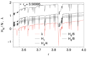
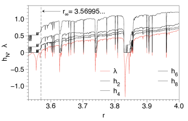
Figure 3: Block entropies of the degree sequence $\{k_{i}\}$ as a function of the bifurcation parameter, as obtained from the HVG of a time series of the logistic map $x_{t+1}=rx_{t}(1-x_{t})$. Left: Normalised entropies $H_{N}/N$ for different block sizes $N$. Right: Differential entropies $h_{N}=H_{N}-H_{N-1}$ for different block sizes $N$. In addition, the figures contain the Lyapunov exponent $\lambda$ of the map, cf. figure 2.

III.2 Graph theoretic block entropies

In direct analogy to the definition of a map’s block entropy, see eq.(2), we can define the HVG-block entropy as the block entropy of a particular degree sequence. In the case of the standard degree sequence $\{k_{i}\}$, this entropic quantity reads

$$H_{N}=-\sum_{\text{blocks}}P(k_{1},\dots,k_{N})\ln P(k_{1},\dots,k_{N}),$$ (4)

where the summation is performed over all admissible block strings of size $N$, $(k_{1},\dots,k_{N})$, and $P(k_{1},k_{2},\dots,k_{N})$ denotes the frequency of occurrence of the degree sequence $(k_{1},\dots,k_{N})$. Similarly for the out-degree sequence $\{k_{i}^{\text{out}}\}$, we define

$$H^{\text{out}}_{N}=-\sum_{\text{blocks}}P(k^{\text{out}}_{1},\dots,k^{\text{out}}_{N})\ln P(k^{\text{out}}_{1},\dots,k^{\text{out}}_{N})\,.$$ (5)

The differential block entropy $h_{N}$ is defined in direct equivalence to its counterpart in the map, $h_{N}=H_{N}-H_{N-1}$ and we are again interested in the limits $\lim_{\rightarrow\infty}H_{N}/N$ and $\lim_{N\rightarrow\infty}h_{N}$, see figure 3. Fortunately, Jensen’s inequality and Fekete’s lemma ensures the existence of limits, as before.

At a phenomenological level, the numerical results displayed in figure 3 suggest that the entropy defined on the basis of node degree sequences shows striking similarity to the entropy defined with respect to generating partitions of the phase space. In particular, we obtain expressions which seem to converge in a monotonic decreasing way towards the Lyapunov exponent of the map (and this also holds for the out-degree sequence, see figure 11). In fact, it has been pointed out recently Route1 ; PLOS that $H_{1}$, which is nothing but the Shannon entropy over a graph’s degree distribution $P(k)$, is qualitatively similar to the Lyapunov exponent $\lambda$ in the Feigenbaum scenario. Hence, it seems sensible to investigate to which extent the degree sequence shares properties of symbolic dynamics. Among others we will discuss whether the degree sequence provide a partition of the phase space, whether this partition finally determines a phase space point, and whether the statistical properties of the degree sequence give additional nontrivial insight into the dynamics of the map $f$.

IV The horizontal visibility algorithm and symbolic dynamics

For the following considerations we will focus exclusively on the fully chaotic logistic map $f(x)=4x(1-x)$. Large parts of our considerations apply to general parameter values $r<4$ if a suitable pruning of the symbolic dynamics will be taken into account. Our main concern is the question whether the degree sequence induces an effective partition of phase space. For this purpose we will first clarify to which extent node degrees can be considered as functions of the initial condition and whether the properties of such a function are amenable to a theoretical investigation.

IV.1 Node degrees as phase space functions

Given a time series, the node degree $k_{t}$ of a datum $x_{t}$ is easily obtained from the degree sequence of the graph. We can therefore numerically reconstruct $k(x)$ which plots the node degree as a function of the phase space coordinate. We have generated both the HVG and its directed version, associated to a time series of $10^{5}$ data from a fully chaotic ($r=4$) logistic map. In the left panel of figure 4 we then plot $k(x)$, whereas in the right panel of the same figure the corresponding out-degree function $k^{\text{out}}(x)$ is plotted.

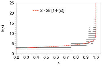
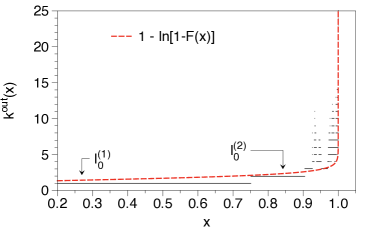
Figure 4: Node degree $k(x)$ in the case of a fully chaotic ($r=4$) logistic map as obtained from the HVG of a time series (left). Analogous plot for the out-degree $k^{\text{out}}(x)$ (right). The labels used for enumerating the piecewise constant branches will be introduced in the main text. Broken lines show the analytical estimates, eqs.(8) and (9).

As expected, $k(x)$ is a multivalued function since the logistic map is not invertible. Interestingly, $k^{\text{out}}(x)$ seems to be single-valued, although the shape is highly heterogeneous, particularly in the region closer to the upper bound of the interval. A zoom of this plot close to $x=1$ is depicted in figure 5, highlighting its complex structure. Before we proceed to evaluate this intricate structure, let us first focus on the overall trend of the two functions which can be captured by a simple stochastic argument. Assuming that we can neglect correlations in the chaotic time series we can model such a series as a set of uncorrelated random variables with probability distribution $\rho(x)=[\pi\sqrt{x(1-x)}]^{-1}$ (i.e. the invariant measure of the map). It has been proven PRE that under such assumptions, the degree distribution conditioned to $x$ is given by

$$P(k|x)=\sum_{j=0}^{k-2}\frac{(-1)^{k-2}}{j!(k-2-j)!}[1-F(x)]^{2}\{\ln[1-F(x)]\}^{k-2}.$$ (6)

A similar expression applies for the out-degree distribution nonlinearity ,

$$P(k^{\text{out}}|x)=P(k^{\text{in}}|x)=\frac{(-1)^{k-1}}{(k-1)!}[1-F(x)]\{\ln[1-F(x)]\}^{k-1},$$ (7)

where $F(x)=\int_{0}^{x}\rho(x^{\prime})dx^{\prime}$ is the cumulative distribution function of the underlying density. Accordingly, one can extract an ’average function’ which for the uncorrelated series reads

$$\langle k(x)\rangle=\sum_{k=2}^{\infty}kP(k|x)=2-2\ln(1-F(x))$$ (8)

and

$$\langle k^{\text{out}}(x)\rangle=\langle k^{\text{in}}(x)\rangle=\sum_{k=1}^{\infty}kP(k^{\text{out}}|x)=1-\ln(1-F(x)).$$ (9)

A comparison of eqs.(8) and (9) with the numerical estimates of $k(x)$ and $k^{\text{out}}(x)$ is shown in figure 4 with $F(x)=1/2+\arcsin(2x-1)/\pi$. It is interesting to see that the analytic prediction for the logistic map produces large values for the node degree only in the vicinity of $x=1$.

Figure 5: A detailed view of $k^{\text{out}}(x)$ for the fully chaotic logistic map (cf. figure 4). The labels used for enumerating the piecewise constant branches will be introduced in the main text. Vertical lines correspond to initial conditions which result in motifs with an unbounded out-degree and and unbounded number of hidden nodes, see the main text.

IV.2 Motifs

A closer look at $k^{\text{out}}(x)$ reveals that this is a piecewise constant function of the initial condition, see figure 5. In fact, such a property is not really a surprise since any initial condition determines uniquely a forward orbit and thus all the outgoing links from the seed node. With a slight abuse of notation, we call the subgraph obtained from an orbit of $p+1$ data such that there is a link between the initial and final data a graph motif (note that $p$ considers both the visible and hidden nodes as well, see figure 6 for illustration). The concept is closely related but not totally identical to the so-called sequential motifs introduced recently motifs .
In formal terms, a motif is a (finite) sequence of $p+1$ orbit points $(x_{0},x_{1},\ldots,x_{p})$ such that $x_{0}\leq x_{p}$ and $x_{0}>x_{\ell}$ for $1\leq\ell\leq p-1$. For an orbit of $p+1$ data, we say that the length of the associated motive is $p$. The ordering of the intermediate points $x_{\ell}$ determines the visibility, the outgoing links, and thus the out-degree $k^{\text{out}}(x_{0})$. By studying motifs we are therefore able to uncover the structure of the function $k^{\text{out}}(x)$ as follows: we will first locate the sets of initial conditions which give rise to particular motif. These sets will be shown to be subintervals labelled ${\cal I}_{\bf x}^{(p)}$ for the motif of length $p$, where the specific labeling $\bf x$ will be made evident below (see figure 6 for all motifs of length $p\leq 4$). We will be able to associate a specific out-degree to each subinterval ${\cal I}_{\bf x}^{(p)}$ such that

$$[0,1]=\bigcup_{p,{\bf x}}{\cal I}_{\bf x}^{(p)}.$$

This phase space partition will then yield, in principle, a way to reconstruct $k^{\text{out}}(x_{0})$ and thus build up the effective symbolisation that we are looking for.

Figure 6: A sketch of all motifs of the fully chaotic logistic map up to length $p=4$. Visible/hidden nodes are indicated by full/open symbols (cf. figure 1). The labels will be introduced and explained in the main text.

IV.3 motifs of short length $p\leq 4$

We start by considering all admissible motifs up to length $p=4$, these are sketched in figure 6. Note that some motifs are not appearing, for instance the one for which $x_{0}>x_{1}>x_{2},\ x_{0}<x_{3}$ is forbidden as for the fully chaotic logistic map it is not possible to find three consecutive data in monotonically decreasing order. In what follows we will explicitly compute the sets of initial conditions that give rise to these motifs along with the relevant notation.

IV.3.1 $p=1$:

Given the logistic map $f(x)=4x(1-x)$ the set of points which obeys $x_{0}<f(x_{0})=x_{1}$ is simply the interval

$${\cal I}_{0}^{(1)}=[0,\xi_{2}^{(1)}]$$

bounded by the nontrivial fixed point $\xi_{2}^{(1)}=3/4$ of the map. Here we use the notation $\xi_{k}^{(p)}$ to denote the fixed points of the $p$-th iterate, $f^{(p)}$, sorted by size, where $k$ runs from $1$ to $2^{p}$. Hence $k^{\text{out}}(x)$ takes the value $1$ on the interval ${\cal I}_{0}^{(1)}$, see figure 4. In fact, the intervals $[0,\xi_{2}^{(1)}]$ and $[\xi_{2}^{(1)},1]$ provide a (non generating) Markov partition and the latter interval is mapped onto the former by the map $f$.

IV.3.2 $p=2$:

By construction, a motif of length two requires $x_{0}>x_{1}=f(x_{0})$ and $x_{0}<x_{2}=f(x_{1})$. Clearly $x_{0}\in[\xi_{2}^{(1)},1]$. Furthermore $x_{0}$ cannot exceed the largest of the period two points, $\xi_{4}^{(2)}$ as otherwise the image of $x_{1}$ would be smaller than $\xi_{4}^{(2)}$, and hence smaller than $x_{0}$. In addition, values $x_{0}$ smaller than $\xi_{4}^{(2)}$ result in images $x_{1}=f(x_{0})$ which on a further iteration step give a value exceeding $x_{0}$, see as well figure 7. Thus the relevant initial conditions for the motif form again a single interval

$${\cal I}_{0}^{(2)}=[\xi_{3}^{(2)},\xi_{4}^{(2)}]$$

bounded by the two largest fixed points of the second iterate, if we keep in mind that $\xi_{3}^{(2)}=\xi_{2}^{(1)}$.

Figure 7: Fully chaotic logistic map with nontrivial fixed point $\xi_{2}^{(1)}$ and unstable period two orbit $\xi_{2}^{(2)}$, $\xi_{4}^{(2)}$.

There are no further motifs (i.e. motifs with hidden nodes) which result in an out-degree $k^{\text{out}}(x)=2$, and the reason is simple: if we had a hidden node in such a structure, it would require iterates of the form $x_{0}>x_{1}>x_{2}$. But, again, the logistic map does not allow for a time series of three consecutive decreasing values. $x_{0}>x_{1}$ requires $x_{0}\in[\xi_{2}^{(1)},1]$ so that $x_{1}\in[0,\xi_{2}^{(1)}]$. If $x_{1}<1/2$ then the image obeys $x_{2}>x_{1}$ as the logistic map is increasing. If $x_{1}\geq 1/2$ then $x_{2}\in[\xi_{2}^{(1)},1]$ and again $x_{2}>x_{1}$.

We conclude that the single motif with $p=2$ captures at once all cases with out-degree two and therefore $k^{\text{out}}(x)=2$ on the interval ${\cal I}_{0}^{(2)}$ (see figures 4 and 5).

IV.3.3 $p=3$

Since a decreasing sequence of three consecutive nodes is forbidden, the initial part of the motif has to obey $x_{1}<x_{2}<x_{0}$. With the additional and necessary condition $x_{0}\leq x_{3}$, these inequalities determine the motif uniquely, which therefore lacks hidden nodes (see figure 6). To compute the set of initial conditions that gives rise to this motif, observe the necessary condition $x_{0}\leq x_{3}=f^{(3)}(x_{0})$. Hence, the set has to be contained in those intervals where the third iterate exceeds the diagonal, see figure 8. These four intervals are bounded by periodic points of order three, $[\xi_{2k-1}^{(3)},\xi_{2k}^{(3)}]$ where $1\leq k\leq 4$. Within the rightmost interval bounded by the largest and the second largest periodic point, the lower order iterates $f^{(m)}(x)$ with $m=1,2$ have a well defined order, i.e. their graphs do not cross (for a formal proof in the general setting see below), and the iterates follow the order specified by the motif, $f(x)<f^{(2)}(x)<x<f^{(3)}(x)$. For all the other intervals the third iterate is not even visible as a lower iterate exceeds the initial value, $f(x)>x$. Hence, the set of initial conditions giving rise to the unique motif of length $p=3$ is given by

$${\cal I}_{L}^{(3)}=[\xi_{7}^{(3)},\xi_{8}^{(3)}].$$

While this set and the corresponding motif gives rise to a node with out-degree three, there are now additional motifs and initial conditions which will result in the same node degree, as we will discover shortly.

Figure 8: Third iterate (blue, thick line) and first and second iterate (red and cyan, thin lines) of the fully chaotic logistic map. Full symbols indicate the 8 period-three points, $\xi_{k}^{(3)}$.

IV.3.4 $p=4$

Since a necessary condition for a motif of length $p=4$ is given by $x_{0}\leq f^{(4)}(x_{0})$ we will look at the graph of the iterates $f^{(k)}$ for $k=1,2,3,4$, see figure 9. As in the previous case the condition $x\leq f^{(4)}(x)$ determines eight intervals bounded by points of period four, $[\xi_{2k-1}^{(4)},\xi_{2k}^{(4)}]$ with $1\leq k\leq 8$. Within any interval which obeys the necessary condition $x\leq f^{(4)}(x)$ the lower order iterates $f^{(m)}(x)$, $m=1,2,3$ have a well defined order, i.e., their graphs do not cross. Otherwise we would have $f^{(m_{1})}(x)=f^{(m_{2})}(x)$ for some value $x$ in the interval, i.e., a periodic orbit of period $|m_{2}-m_{1}|<4$. Then however $x_{4}$ cannot not be visible, as its value would be taken by one of the previous iterates.

Figure 9: Fourth iterate (blue, thick line) and lower order iterates (bronze, red and cyan, thin lines) of the fully chaotic logistic map, in the region beyond the period two orbit. Vertical lines indicate intervals determined by the largest period four points $\xi_{k}^{(4)}$.

It is obvious that we only need to consider the region beyond the period-two orbit, $x>\xi_{2}^{(2)}$, as otherwise either $f(x)>x$ or $f^{(2)}(x)>x$. Only the two largest intervals

$${\cal I}_{LL}^{(4)}=[\xi_{7}^{(4)},\xi_{8}^{(4)}]$$

and

$${\cal I}_{LR}^{(4)}=[\xi_{5}^{(4)},\xi_{6}^{(4)}]$$

obey the visibility constraints for intermediate nodes, i.e., $f^{(k)}(x_{0})=x_{k}<x_{0}$ for $1\leq k\leq 3$ (see the section below for the notation used to label the intervals). These intervals give rise to two motifs, see figure 6, with the nodes ordered according to $x_{1}<x_{2}<x_{3}<x_{0}<x_{4}$ or $x_{1}<x_{3}<x_{2}<x_{0}<x_{4}$. It is in fact rather obvious that only two motifs exist as the three initial nodes have to obey $x_{1}<x_{2}<x_{0}$ as already mentioned above. Thus, there are just two possibilities left for the visibility of the third node. The case $p=4$ is the first instance of a motif with a hidden node: one motif yields out-degree three, while the other one yields out-degree four.

In fact, there are no further motifs resulting in an out-degree three. Hence, the set of initial conditions giving rise to out-degree three consists of two disjoint intervals

$$\{x_{0}|k^{\text{out}}(x_{0})=3\}={\cal I}_{L}^{(3)}\cup{\cal I}_{LR}^{(4)},$$

see as well figure 5. To prove this claim we need to show that for a sequence of nodes with $x_{1}<x_{3}<x_{2}<x_{0}$ the following point $x_{4}$ cannot be a hidden node with $x_{4}<x_{2}$. Since $x_{3}<x_{2}$ we know, see the discussion of the logistic map in the previous section, that $x_{2}$ is contained in $[\xi_{2}^{(1)},1]$, i.e., $x_{2}$ is bounded from below by the nontrivial fixed point $x_{2}>\xi_{2}^{(1)}$. Since $x_{2}<x_{0}$ the graph of the second iterate $f^{(2)}$ (see, e.g., figure 8) tells us that $x_{0}>\xi_{4}^{(2)}$ and hence $x_{2}=f^{(2)}(x_{0})<\xi_{4}^{(2)}$. Thus $x_{2}$ is contained in the interval $[\xi_{2}^{(1)},\xi_{4}^{(2)}]$ but on this interval the graph of the second iterate is above the diagonal, $f^{(2)}(x)>x$. Hence $x_{4}>x_{2}$.

motifs of length $p>4$ become increasingly difficult to construct by explicit methods. Thus, a more systematic approach is needed.

IV.4 motifs without hidden nodes

Before we address the general case, let us first focus on motifs of length $p$ where all nodes are visible (no hidden nodes), i.e. $x_{1}<x_{2}<\ldots<x_{p-1}<x_{0}<x_{p}$. In other words, in these motifs all intermediate nodes constitute an increasing subsequence. In what follows we analytically obtain the sets of initial conditions yielding these motifs.

We start by observing that the $p$-th iterate $f^{(p)}$ is a $p$-modal function with $2^{p-1}$ maxima at one and $2^{p-1}+1$ minima at zero. Between extrema, branches are monotonic. The $p$-th iterate has $2^{p}$ fixed points, $\xi^{(p)}_{k}$ where $1\leq k\leq 2^{p}$, and given the properties mentioned before the inequality $f^{(p)}(x)>x$ is satisfied on the $2^{p-1}$ intervals $[\xi_{2k-1}^{(p)},\xi_{2k}^{(p)}]$ where $1\leq k\leq 2^{p-1}$. As already shown above, on any interval which obeys the visibility condition $x_{0}\leq x_{p}=f^{(p)}(x_{0})$ the lower order iterates $f^{(m)}$ with $1\leq m\leq p-1$ have a well defined order, i.e., these functions do not intersect. In what follows we will only consider these intervals.

The ordering of the branches of the iterates is different for different intervals $[\xi_{2k-1}^{(p)},\xi_{2k}^{(p)}]$. To prove this claim we need to resort to symbolic dynamics. Within $[\xi_{2k-1}^{(p)},\xi_{2k}^{(p)}]$ there is a single point $x_{m}$ where $f^{(p)}$ takes its maximum, i.e., $f^{(p)}(x_{m})=1$. The orbit of this point, i.e. the sequence $f^{(k)}(x_{m})$ with $1\leq k\leq p-1$ determines the ordering of the branches. Similarly, if the ordering of the branches is given we can compute the value of $x_{m}$ by backward iteration. The condition $f^{(p)}(x_{m})=1$ means $f^{(p-1)}(x_{m})=1/2$. The value of $f^{(p-2)}(x_{m})$ is the preimage of $1/2$. The relative ordering of the iterates $f^{(p-2)}$ and $f^{(p-1)}$ tells us whether $f^{(p-2)}(x_{m})$ is smaller or larger than $f^{(p-1)}(x_{m})=1/2$, i.e., it tells us whether to apply the left of the right branch of the inverse function $f^{-1}$. Hence we can uniquely compute the entire sequence $f^{(k)}(x_{m})$ as the relative ordering of the iterates $f^{(k)}$ and $f^{(p-1)}$ tells us in each step which branch of the inverse function has to be applied. That in turn implies that two different intervals must have two different orderings of iterates. Otherwise one would obtain the same value for $x_{m}$, but the two intervals do not have a point in common. In summary, we can label each of the intervals $[\xi_{2k-1}^{(p)},\xi_{2k}^{(p)}]$ by a symbol sequence of L’s and R’s such that $f^{(k)}(x_{m})\in{\cal I}_{L/R}$ for $1\leq k\leq p-2$. This notation has been already used in the previous discussion of special cases (see figure 6).

With these preliminary considerations we are now able to evaluate motifs without hidden nodes $x_{1}<x_{2}<\ldots<x_{p-1}<x_{0}<x_{p}$. In this case the corresponding orbit $x_{m},f(x_{m}),\ldots,f^{(p-2)}(x_{m}),f^{(p-1)}(x_{m})=1/2,f^{(p)}=1$ has a monotonic increasing part $f(x_{m})<f^{(2)}(x_{m})<\ldots<f^{(p-2}(x_{m})<1/2$, meaning that all the orbit points are preimages of $1/2$ by using the left branch of the inverse function. Hence, the value obtained for $f(x_{m})$ is the smallest possible value among all the intervals $[\xi_{2k-1}^{(p)},\xi_{2k}^{(p)}]$ and in turn $x_{m}$ is the largest possible value. Thus the interval giving the motive without hidden nodes is the rightmost interval $[\xi_{2^{p}-1}^{(p)},\xi_{2^{p}}^{(p)}]$. According to our notation it is labelled by ${\cal I}^{(p)}_{LL\ldots L}$ (see as well figure 6). Finally we have shown that

$${\cal I}^{(p)}_{LL\ldots L}=[\xi_{2^{p}-1}^{(p)},\xi_{2^{p}}^{(p)}].$$

As these motifs lack hidden nodes, all initial conditions in ${\cal I}^{(p)}_{LL\ldots L}$ have an associated node with out-degree $p$.

The weight of motifs without hidden nodes:

To figure out which part of the phase space is covered by motifs without hidden nodes let us consider in more in detail the intervals ${\cal I}^{(p)}_{LL\ldots L}$. Denoting the length of an interval by $|[a,b]|=|b-a|$ the ratio

$$\zeta(p)=\frac{|{\cal I}^{(p)}_{LL\ldots L}|}{|{\cal I}^{(p-1)}_{LL\ldots L}|},\ (p\geq 2)$$ (10)

measures the shrinking rate of the intervals of initial conditions resulting in motifs of length $p$ without hidden nodes. Interestingly, numerical evidence suggests that this rate rapidly converges to

$$\lim_{p\to\infty}\zeta(p)\approx 0.125\,.$$

One can compute this limit analytically building on the conjugation to the tent map, which tells us that

$$\xi_{2^{p}}^{(p)}=\sin^{2}\bigg{(}\frac{\pi}{2}\frac{2^{p}}{2^{p}+1}\bigg{)};\ \xi_{2^{p}-1}^{(p)}=\sin^{2}\bigg{(}\frac{\pi}{2}\frac{2^{p}-2}{2^{p}-1}\bigg{)}\,.$$

Therefore

$$\lim_{p\to\infty}\zeta(p)=\lim_{p\to\infty}\frac{\sin^{2}\bigg{(}\frac{\pi}{2}\frac{2^{p}}{2^{p}+1}\bigg{)}-\sin^{2}\bigg{(}\frac{\pi}{2}\frac{2^{p}-2}{2^{p}-1}\bigg{)}}{\sin^{2}\bigg{(}\frac{\pi}{2}\frac{2^{p-1}}{2^{p-1}+1}\bigg{)}-\sin^{2}\bigg{(}\frac{\pi}{2}\frac{2^{p-1}-2}{2^{p-1}-1}\bigg{)}}=\frac{1}{8}\,.$$

Similarly, if $\mathbb{P}^{(0)}(p)$ defines the probability of finding a certain symbol $k^{\text{out}}=p$ without hidden nodes, then

$$\mathbb{P}_{0}(p)=\int_{\xi_{2^{p}-1}^{(p)}}^{\xi_{2^{p}}^{(p)}}\frac{dx}{\pi\sqrt{x(1-x)}}=$$

$$\frac{\arcsin(2\xi^{(p)}_{2^{p}}-1)-\arcsin(2\xi^{(p)}_{2^{p}-1}-1)}{\pi}=\frac{2}{4^{p}-1}$$

giving a rigorous lower bound on the exponential decay of the degree distribution of the HVG. Accordingly, the total contribution of motifs without hidden nodes, $\Lambda_{0}$, can be defined as

$$\Lambda_{0}=\sum_{p=1}^{\infty}\mathbb{P}_{0}(p)=\sum_{p=1}^{\infty}\frac{2}{4^{p}-1}\,$$ (11)

This series can be written in terms of the q-polygamma function, and the expression has some similarity to the Erdös-Borwein constant . The value of $\Lambda_{0}$ is irrational by a theorem of Borwein borwein , but apart from this fact not much seems to be known about this constant. We find that $\Lambda_{0}\approx 0.842195\dots$, converging after $p=11$. This means that up to $84\%$ of all initial conditions generate trajectories whose associated out-degree sequence lacks hidden nodes.

IV.5 General motifs, periodic points, and symbolic encoding

To give a complete description of motifs of length $p>2$ we need a few more details about symbolic dynamics. To keep the presentation self-contained we first summarise a few facts for the convenience of the reader, even though more comprehensive reviews can be found in textbooks CE .

Given the canonical partition of the interval in terms of two subintervals ${\cal I}_{L}=[0,1/2]$ and ${\cal I}_{R}=[1/2,1]$ we can (essentially) associate to each orbit of the map $(x_{0},x_{1},\ldots)$, that means to each initial condition $x_{0}$, a symbol sequence $\sigma_{0},\sigma_{1},\ldots$ consisting of symbols $\sigma_{k}\in\{L,R\}$, such that the symbols tell us the location of the orbit points, $x_{k}\in{\cal I}_{\sigma_{k}}$. For the case of the fully chaotic logistic map all symbol sequences are indeed admissible. Other parameter values can be covered as well by pruning the set of admissible symbol sequences.

Ordering of symbol sequences:

Given two initial conditions $x_{0}$ and $\bar{x}_{0}$ for which $x_{0}<\bar{x}_{0}$, this usual order in phase space $x_{0}<\bar{x}_{0}$ induces a corresponding order $\prec$ among symbol sequences, which is essentially a binary order taking into account that one branch of the logistic map is decreasing. To be slightly more specific, such ordering relation is defined as follows:
(i) $L\sigma_{1}\sigma_{2}\ldots\prec R\bar{\sigma}_{1}\bar{\sigma}_{2}\ldots$. Furthermore,
(ii) if the first $N$ symbols of two sequences coincide $\sigma_{0}\ldots\sigma_{N-1}=\bar{\sigma}_{0}\ldots\bar{\sigma}_{N-1}$ and if this string contains an even number of R’s, then $\sigma_{0}\ldots\sigma_{N-1}L\ldots\prec\sigma_{0}\ldots\sigma_{N-1}R\ldots$. Otherwise,
(iii) if the string contains an odd number of R’s then $\sigma_{0}\ldots\sigma_{N-1}R\ldots\prec\sigma_{0}\ldots\sigma_{N-1}L\ldots$.

Maximal sequences:

This ordering of symbol sequences is defined in such a way that it coincides with the order of the corresponding initial conditions. Periodic symbol sequences, $\sigma_{k+p}=\sigma_{k}$ for $k\geq 0$, correspond to phase space points of period $p$. We will use the notation $\overline{\sigma_{0}\ldots\sigma_{p-1}}$ to denote periodic symbol sequences. A periodic sequence $\overline{\sigma_{0}\ldots\sigma_{p-1}}$ is said to be a maximal symbol sequence if $\sigma_{k}\sigma_{k+1}\ldots\prec\sigma_{0}\sigma_{1}\ldots$ for $1\leq k\leq p-1$. In geometric terms a maximal periodic symbol sequence corresponds to a period $p$ point $x_{0}$ of the map, such that $x_{0}$ is the largest value among all iterates, $x_{0}>x_{k}$ for $1\leq k\leq p-1$.

Encoding of motifs with length $p>2$:

Using symbolic dynamics we are now equipped with the necessary tools to rephrase the results which have been implicitly obtained in the previous sections. For a given motif of length $p$ with a given order of nodes the corresponding initial conditions $x_{0}$ are contained in an interval $[\xi_{2k-1}^{(p)},\xi_{2k}^{(p)}]$ whose endpoints are periodic points of order $p$. If $x_{0}\in[\xi_{2k-1}^{(p)},\xi_{2k}^{(p)}]$ scans the interval the iterates $x_{k}=f^{k}(x_{0})$ for $1\leq k\leq p-2$ never become $1/2$, i.e., we can attach a unique symbol $\sigma_{k}\in\{L,R\}$ to $x_{k}$ according to $x_{k}\in{\cal I}_{\sigma_{k}}$. When $x_{0}$ scans the interval the iterate $x_{p-1}=f^{(p-1)}(x_{0})$ crosses $1/2$ once, meaning that the corresponding symbol $\sigma_{p-1}$ changes. Finally the visibility conditions ensure that $x_{0}$ and $x_{p}$ are contained in ${\cal I}_{R}$ (recall that we consider the case $p>2$) so that $\sigma_{0}=\sigma_{p}=R$. Hence the two periodic points which are the boundaries of the interval of the motif have symbol code $\overline{R\sigma_{1}\ldots\sigma_{p-2}L}$ and $\overline{R\sigma_{1}\ldots\sigma_{p-2}R}$ where the finite symbol string $\sigma_{1}\ldots\sigma_{p-2}$ is the unique identifier of the motive

$${\cal I}^{(p)}_{\sigma_{1}\ldots\sigma_{p-2}}=[\xi_{2k-1}^{(p)},\xi_{2k}^{(p)}],\quad(p>2)\,.$$ (12)

The two periodic symbol strings are maximal sequences, since visibility requires that $x_{0}=x_{p}$ is the largest value in the respective periodic orbit.

Properties of $k^{\text{out}}(x)$:

The theoretical analysis displayed above give us a workable solution to label all motifs in terms of subintervals, i.e. we are able to associate to each motif a set of initial conditions. That is, we have been able to make a partition of the phase space into a countable union of subintervals, and we indeed control the location of each of the (countably infinite) subintervals. Moreover, $k^{\text{out}}(x)$ takes a constant value on each of these subintervals. However, there does not seem to be a simple recipe relating the properties of the symbol string with the actual out-degree of the specific motif. In particular, that means that we can find many different (disjoint) subintervals whose initial conditions yield the same out-degree. Because of this, the full explicit construction of $k^{\text{out}}(x)$ is currently out of reach. Notwithstanding, we are able to explore some further properties of this function, as follows.

We first claim that the node degree of motifs is not bounded and the function $k^{\text{out}}(x)$ can take arbitrarily large values in any small neighbourhood of particular $x$ values. The simplest case has been considered in the previous section but there are less trivial cases. Consider the orbit $x_{0},x_{1},\xi_{2}^{(1)},\xi_{2}^{(1)},\ldots$ which ends up in the nontrivial fixed point after two iteration steps (see figure 10), i.e., $x_{0}=1/2+\sqrt{3}/4=.9330\ldots$. Changing the value of $x_{0}$ by a very small amount the orbit will slowly be repelled from the unstable fixed point so that nodes $x_{0}$, $x_{1}$ and every other of the following iterates will be visible until finally the motive terminates with a value exceeding $x_{0}$. By making the increment as small as we wish we can make the node degree as large as we want. Hence $k^{\text{out}}(x)$ is unbounded at $x=1/2+\sqrt{3}/4$ as can be seen as well in figure 5. We can easily construct a countable infinite set of such $x$-values, related to unstable orbits of higher period.

Figure 10: Orbits related to motifs with an arbitrary large number of nodes (cyan, bottom labels) and motifs with an arbitrary large number of hidden nodes (cyan and bronze, top labels).

Second, we then claim that there are motifs with an arbitrarily large number of hidden nodes. Consider for instance the orbit of $x_{0}=0.9484\ldots$ which ends up in the nontrivial fixed point $\xi_{2}^{(1)}=3/4$ after five iterations and whose transient obeys the pattern $x_{1}<x_{4}<x_{2}<x_{3}$ see figure 10. Nodes $x_{1}$, $x_{2}$ and $x_{3}$ are visible (cf. ${\cal I}_{LL}^{(4)}$ in figure 6) and $x_{4}$ and the fixed point are invisible. If we change $x_{0}$ by a small amount the orbit will spiral around the unstable fixed point generating a large number of invisible nodes in the motive, until finally the motive terminates with a value larger than the initial value. As in the previous case in any open neighbourhood of $x_{0}=0.9484\ldots$ we can find motifs with as many hidden nodes as we want. In particular, our argument implies that there is a countably infinite set of motifs with out-degree $p\geq 4$. Hence, the set of values where $k^{\text{out}}(x)=4$ consists of a countably infinite union of intervals, see figure 5, and there is no obvious way to characterise this set.

V Discussion

In this work we have explored the properties of the degree sequence of horizontal visibility graphs associated with chaotic time series using symbolic dynamics. For concreteness, we have focused on the logistic map $x_{t+1}=rx_{t}(1-x_{t})$, a canonical interval map showing transition from regular to chaotic dynamics as $r$ is varied. Numerically, we have shown that the Lyapunov exponent of the logistic map is well approximated asymptotically by a sequence of block entropies on both the degree and out-degree sequences. Via Pesin theorem, this suggests that this sequence of entropies is converging to the Kolmogorov-Sinai entropy of the map, and therefore constitutes a combinatoric version of the metric dynamical invariant. Furthermore, this connection suggests that the horizontal visibility graph is inducing a symbolic dynamics and effectively produces partitions of the interval which could be generating. Note that the algorithm itself does not pre-define the alphabet (i.e. the number of different degrees), and the way it constructs the degree sequence from the original time series does not suggest a priori that there might be an underlying partition of the phase space operating at all. So an explicit construction of such partition would constitute an unexpected and nontrivial result.

Figure 11: $h^{\text{out}}_{N}$ for different block sizes $N$, as a function of the map’s parameter $r$, where we appreciate how the successive approximations to the entropy rate converge to the Lyapunov exponent $\lambda$ of the map, for all values of $r$.

To further explore this possibility, we have elaborated on the explicit construction of such effective partition in a sequential way. Unlike the degree, we have shown that the out-degree is a well defined phase space function and the level curves, i.e., the sets on which the out-degree takes a specific value, provide a countable partition of the phase space. Level sets for out-degree one, two, and three are either intervals or the union of two intervals, while all sets of degree larger than three consist of a countable infinite union of subintervals. We have proved that all subintervals are bounded by periodic points and each subinterval can be labelled according to a so-called maximal symbol sequence. We found that the vast majority of the phase space is covered by sets with corresponding low out-degree or by motifs without any hidden nodes, where explicit calculations are possible.

Furthermore, the entropy based on the out-degree sequence, eq.(5), shows a striking similarity to the Kolmogorov-Sinai entropy (see figure 11). In fact, the out-degree provides a partition of the phase space, and considering out-degree sequences implicitly provides a dynamic refinement of this partition, as in the case of the Kolmogorov-Sinai entropy. The set of phase space points giving rise to a finite degree sequence $k^{\text{out}}_{1},k^{\text{out}}_{2},\dots,k^{\text{out}}_{N}$ is the intersection of the sets such that $f^{(m-1)}(x)$ is contained in the part with out-degree $k^{\text{out}}_{m}$ for $1\leq m\leq N$. Such a construction is precisely the definition of a dynamically refined partition. A formal proof along standard lines, to show that the entropy based on degree distributions equals the Kolmogorov-Sinai entropy, would amount to establish the generating property of the underlying partition. However the partition defined by the out-degree can hardly be generating in the topological sense as the map is non monotonic on the part ${\cal I}^{(1)}_{0}$. Nevertheless, out-degree sequences can be efficiently used to count periodic orbits and thus share properties of a generating partition. Obviously any periodic orbit results in a periodic degree sequence of the same period. In addition, we have shown that any motif ${\cal I}^{(p)}_{\underline{\sigma}}$ has a characteristic ordering of branches of iterates, and this ordering is different for each motif. The ordering of these branches determines the degree sequence, so that the degree sequence is a fingerprint of the motif. If we confine to periodic degree sequences and periodic orbits we have thus shown that a periodic degree sequence is a specific property of the two periodic orbits which constitute the boundary points of the motif, i.e., the mapping from degree sequences to periodic orbits is one to two.

Hence, the entropy based on out-degrees is closely related, but not identical, to well established concepts in dynamical systems theory. A similar statement is of course valid for the undirected degree sequence or for the in-degree sequences. From a rigorous perspective their relation to topological properties of the underlying dynamics remains as an open problem, even though we have compelling numerical and analytic evidence that all the entropy values coincide. Other interesting open questions include the extension of this technique to chaotic maps in higher dimensions Enzo .

- (1) L. Lacasa, B. Luque, F. Ballesteros, J. Luque, J.C. Nuño, From time series to complex networks: the visibility graph, Proc. Natl. Acad. Sci. USA 105, 13 (2008).
- (2) B. Luque, L. Lacasa, J. Luque, F.J. Ballesteros, Horizontal visibility graphs: exact results for random time series, Phys. Rev. E 80, 046103 (2009).
- (3) G. Gutin, M. Mansour, S. Severini, A characterization of horizontal visibility graphs and combinatorics on words, Physica A 390, 12 (2011).
- (4) L. Lacasa, On the degree distribution of horizontal visibility graphs associated to Markov processes and dynamical systems: diagrammatic and variational approaches, Nonlinearity 27, 2063-2093 (2014).
- (5) B. Luque, L. Lacasa, Canonical horizontal visibility graphs are uniquely determined by their degree sequence, Eur. Phys. J. Sp. Top. 226, 383 (2017).
- (6) L. Lacasa, B. Luque, J. Luque, J.C. Nuno, The Visibility Graph: a new method for estimating the Hurst exponent of fractional Brownian motion, EPL 86, 30001 (2009).
- (7) L. Lacasa, R. Toral, Description of stochastic and chaotic series using visibility graphs, Phys. Rev. E 82, 036120 (2010).
- (8) B. Luque, L. Lacasa, F.J. Ballesteros, A. Robledo, Analytical properties of horizontal visibility graphs in the Feigenbaum scenario, Chaos 22, 013109 (2012).
- (9) B. Luque, F.J. Ballesteros, A.M. Nuñez and A. Robledo, Quasiperiodic Graphs: Structural Design, Scaling and Entropic Properties, J. Nonlinear Sci. 23 (2013) 335-342.
- (10) A. Nuñez, B. Luque, L, Lacasa, J.P. Gomez, A. Robledo, Horizontal Visibility graphs generated by type-I intermittency, Phys. Rev. E 87, 052801 (2013).
- (11) B. Luque, L. Lacasa, F.J. Ballesteros, A. Robledo, Feigenbaum graphs: a complex network perspective of chaos PLoS ONE 6, 9 (2011).
- (12) L. Lacasa and R. Flanagan, Time reversibility from visibility graphs of non-stationary processes Phys. Rev. E 92, 022817 (2015)
- (13) L. Lacasa, A. Nuñez, E. Roldan, JMR Parrondo, B. Luque, Time series irreversibility: a visibility graph approach, Eur. Phys. J. B 85, 217 (2012).
- (14) J.F. Donges, R.V. Donner and J. Kurths, Testing time series irreversibility using complex network methods, EPL 102, 10004 (2013).
- (15) A. Aragoneses, L. Carpi, N. Tarasov, D.V. Churkin, M.C. Torrent, C. Masoller, and S.K. Turitsyn, Unveiling Temporal Correlations Characteristic of a Phase Transition in the Output Intensity of a Fiber Laser, Phys. Rev. Lett. 116, 033902 (2016).
- (16) M. Murugesana and R.I. Sujitha1, Combustion noise is scale-free: transition from scale-free to order at the onset of thermoacoustic instability, J. Fluid Mech. 772 (2015).
- (17) A. Charakopoulos, T.E. Karakasidis, P.N. Papanicolaou and A. Liakopoulos, The application of complex network time series analysis in turbulent heated jets, Chaos 24, 024408 (2014).
- (18) P. Manshour, M.R. Rahimi Tabar and J. Peinche, Fully developed turbulence in the view of horizontal visibility graphs, J. Stat. Mech. (2015) P08031.
- (19) RV Donner, JF Donges, Visibility graph analysis of geophysical time series: Potentials and possible pitfalls, Acta Geophysica 60, 3 (2012).
- (20) V. Suyal, A. Prasad, H.P. Singh, Visibility-Graph Analysis of the Solar Wind Velocity, Solar Physics 289, 379-389 (2014)
- (21) Y. Zou, R.V. Donner, N. Marwan, M. Small, and J. Kurths, Long-term changes in the north-south asymmetry of solar activity: a nonlinear dynamics characterization using visibility graphs, Nonlin. Processes Geophys. 21, 1113-1126 (2014).
- (22) S. Jiang, C. Bian, X. Ning and Q.D.Y. Ma, Visibility graph analysis on heartbeat dynamics of meditation training, Appl. Phys. Lett. 102 253702 (2013).
- (23) M Ahmadlou, H Adeli, A Adeli, New diagnostic EEG markers of the Alzheimer’s disease using visibility graph, J. of Neural Transm. 117, 9 (2010).
- (24) S. Sannino, S. Stramaglia, L. Lacasa, D. Marinazzo. Visibility graphs for fMRI data: multiplex temporal graphs and their modulations across resting state networks Network Neuroscience (in press 2017) bioRxiv 106443.
- (25) J. Iacovacci and L. Lacasa, Sequential visibility-graph motifs, Phys. Rev. E 93, 042309 (2016)
- (26) R. Flanagan and L. Lacasa, Irreversibility of financial time series: a graph-theoretical approach, Physics Letters A 380, 1689-1697 (2016)
- (27) L. Lacasa, V. Nicosia and V. Latora, Network Structure of Multivariate Time Series Sci. Rep. 5, 15508 (2015).
- (28) P. Collet and JP Eckmann, Iterated maps on the interval as dynamical systems (Progress in Physics, Birkhauser 1980).
- (29) P. Collet and JP Eckmann,Concepts and Results in Chaotic Dynamics (Springer, Berlin 2006).
- (30) C. Beck and F. Schlogl, Thermodynamics of chaotic systems (Cambridge University Press 1993)
- (31) JP Crutchfield and NH Packard, Symbolic dynamics of one-dimensional maps: entropies, finite precision, and noise, International Journal of Theoretical Physics 21, 6/7 (1982).
- (32) Y. Pesin, Characteristic Lyapunov exponents and smooth ergodic theory, Uspeki Matematicheskikh Nauk 45, 712 (1977).
- (33) D. Ruelle, An inequality for the entropy of differentiable maps, Bull. Soc. Brasil Math. 9, 331 (1978).
- (34) P. Grassberger and H. Kantz, Generating Partitions for the dissipative Henon map, Phys. Lett. A 113 (1985).
- (35) Y. Oono and M. Osikawa, Chaos in nonlinear difference equations I, Progress in Theoretical Physics 64, 54 (1980).
- (36) F. Ledrappier, Some properties of absolutely continuous invariant measures on an interval, Ergod. Theo. Dyn. Sys. 1, 77 (1981).
- (37) P. Borwein, On the Irrationality of Certain Series, Math. Proc. Cambridge Philos. Soc. 112 (1992) pp. 141-146.