Nonlocal Inpainting of Manifold-valued Data
on Finite Weighted Graphs

Abstract

Recently, there has been a strong ambition to translate models and algorithms from traditional image processing to non-Euclidean domains, e.g., to manifold-valued data. While the task of denoising has been extensively studied in the last years, there was rarely an attempt to perform image inpainting on manifold-valued data. In this paper we present a nonlocal inpainting method for manifold-valued data given on a finite weighted graph. We introduce a new graph infinity-Laplace operator based on the idea of discrete minimizing Lipschitz extensions, which we use to formulate the inpainting problem as PDE on the graph. Furthermore, we derive an explicit numerical solving scheme, which we evaluate on two classes of synthetic manifold-valued images.

1 Introduction

Variational methods and partial differential equations (PDEs) play a key role for both modeling and solving image processing tasks. When processing real world data certain information might be missing due to structural artifacts, occlusions, or damaged measurement devices. Reconstruction of missing image information is known as inpainting task and there exist various variational models to perform inpainting. One successful method from the literature is based on a discretization of the $\infty$-Laplace operator [7]. This idea has been adapted to finite weighted graphs in [10]. The graph model enables to perform local and nonlocal inpainting within the same framework based on the chosen graph construction. Nonlocal inpainting has the advantage of preserving structural features by using all available information in the given image instead of only local neighborhood values.

With the technological progress in modern data sensors there is an emerging field of processing non-Euclidean data. We concentrate our discussion in the following on manifold-valued data, i.e., each data value lies on a Riemannian manifold. Real examples for manifold-valued images are interferometric synthetic aperture radar (InSAR) imaging [14], where the measured phase-valued data may be noisy and/or incomplete. Sphere-valued data appears, e.g., in directional analysis [13]. Another application is diffusion tensor imaging (DT-MRI) [3], where the diffusion tensors can be represented as $3\times 3$ symmetric positive definite matrices, which also constitute a manifold. For such data, there were several variational methods and algorithms proposed to perform image processing tasks, see e.g., [2, 4, 9, 12, 17]. Recently, the authors generalized the graph $p$-Laplacian for manifold-valued data, $1\leq p<\infty$, in [5] and derived an explicit as well as an semi-implicit iteration scheme for computing solutions to related partial difference equations on graphs as mimetic approximation of continuous PDEs. While the previous work concentrated on denoising, the present work deals with the task of image inpainting of manifold-valued data. For this, we extend the already defined family of manifold-valued graph $p$-Laplacians by a new operator, namely the graph $\infty$-Laplacian for manifold valued data. We derive an explicit numerical scheme to solve the corresponding PDE and illustrate its capabilities by performing nonlocal inpainting of synthetic manifold-valued data.

The remainder of this paper is organized as follows: In Sec. 2 we introduce the necessary notations of Riemannian manifolds, finite weighted graphs, and manifold-valued vertex functions. In Sec. 3 we introduce a new graph $\infty$-Laplace operator for manifold-valued data based on the idea of discrete minimizing Lipschitz extensions. Furthermore, we derive an explicit numerical scheme to solve the corresponding PDE $\Delta_{\infty}f=0$ with suitable boundary conditions. In Sec. 4 we apply the proposed method to inpainting of synthetic manifold-valued images. Finally, Sec. 5 concludes the paper.

2 Preliminaries

In this section we first introduce the needed theory and notations on Riemannian manifolds in Sec. 2.1 and introduce finite weighted graphs in Sec. 2.2. We then combine both concepts to introduce vertex functions and tangential edge functions needed for the remainder of this paper in Sec. 2.3. For further details we refer to [5].

2.1 Riemannian manifolds

For a detailed introduction to functions on Riemannian manifolds we refer to, e.g., [1, 11]. The values of the given data lie in a complete, connected, $m$-dimensional Riemannian manifold $\mathcal{M}$ with Riemannian metric $\langle\cdot,\cdot\rangle_{x}\colon\mathrm{T}_{x}\mathcal{M}\times\mathrm{T}_{x}\mathcal{M}\to\mathbb{R}$, where $\mathrm{T}_{x}\mathcal{M}$ is the tangent space at $x\in\mathcal{M}$. In every tangent space $\mathrm{T}_{x}\mathcal{M}$ the metric induces a norm, which we denote by $\lVert\cdot\rVert_{x}$. The disjoint union of all tangent spaces is called the tangent bundle $\mathrm{T}\mathcal{M}\coloneqq\dot{\cup}_{x\in\mathcal{M}}\mathrm{T}_{x}\mathcal{M}$. Two points $x,y\in\mathcal{M}$ can be joined by a (not necessarily unique) shortest curve $\gamma_{\overset{\frown}{x,y}}\colon[0,L]\to\mathcal{M}$, where $L$ is its length. This generalizes the idea of shortest paths from the Euclidean space $\mathcal{M}=\mathbb{R}^{m}$, i.e., straight lines, to a manifold and induces the geodesic distance denoted $d_{\mathcal{M}}\colon\mathcal{M}\times\mathcal{M}\to\mathbb{R}^{+}$. A curve $\gamma$ can be reparametrized such that derivative vector field $\dot{\gamma}(t)\coloneqq\frac{d}{dt}\gamma(t)\in T_{\gamma(t)}\mathcal{M}$ has constant norm, i.e., $\lVert\dot{\gamma}_{\overset{\frown}{x,y}}(t)\rVert_{\gamma_{\overset{\frown}{x,y}}(t)}=1$, $t\in[0,L]$. The corresponding curve then has unit speed. We employ another notation of a geodesic, namely $\gamma_{x,\xi}$, $\xi\in\mathrm{T}_{x}\mathcal{M}$, $x\in\mathcal{M}$, which denotes the locally unique geodesic fulfilling $\gamma_{x,\xi}(0)=x$ and $\dot{\gamma}_{x,\xi}(0)=\xi\in\mathrm{T}_{x}\mathcal{M}$. This is unique due to the Hopf–Rinow Theorem, cf. [11, Theorem 1.7.1]. We further introduce the exponential map $\exp_{x}\colon\mathrm{T}_{x}\mathcal{M}\to\mathcal{M}$ as $\exp_{x}(\xi)=\gamma_{x,\xi}(1)$. Let $r_{x}\in\mathbb{R}^{+}$ denote the injectivity radius, i.e., the largest radius such that $\exp_{x}$ is injective for all $\xi$ with $\lVert\xi\rVert_{x}<r_{x}$. Furthermore, let

$$\mathcal{D}_{x}\coloneqq\bigl{\{}y\in\mathcal{M}:y=\exp_{x}\xi,\text{ for some }\xi\in T_{x}\mathcal{M}\text{ with }\lVert\xi\rVert_{x}<r_{x}\bigr{\}}\ .$$

Then the inverse map $\log_{x}\colon\mathcal{D}_{x}\to\mathrm{T}_{x}\mathcal{M}$ is called the logarithmic map and maps a point $y=\gamma_{x,\xi}(1)\in\mathcal{D}_{x}$ to $\xi$.

2.2 Finite weighted graphs

Finite weighted graphs allow to model relations between arbitrary discrete data. Both local and nonlocal methods can be unified within the graph framework by using different graph construction methods: spatial vicinity for local methods like finite differences, and feature similarity for nonlocal methods. A finite weighted graph $G=(V,E,w)$ consists of a finite set of indices $V=\{1,\ldots,n\}$, $n\in\mathbb{N}$, denoting the vertices, a set of directed edges $E\subset V\times V$ connecting a subset of vertices, and a nonnegative weight function $w\colon E\rightarrow\mathbb{R}^{+}$ defined on the edges of a graph. For an edge $(u,v)\in E$, $u,v\in V$ the node $u$ is the start node, while $v$ is the end node. We also denote this relationship by $v\sim u$. Furthermore, the weight function $w$ can be extended to all $V\times V$ by setting $w(u,v)=0$ when $v\not\sim u$. The neighborhood $\mathcal{N}(u)\coloneqq\{v\in V:v\sim u\}$ is the set of adjacent nodes.

2.3 Manifold-valued vertex functions and tangential edge functions.

The functions of main interest in this work are manifold-valued vertex functions, which are defined as

$$f\colon V\to\mathcal{M},\quad u\mapsto f(u),$$

The range of the vertex function $f$ is the Riemannian manifold $\mathcal{M}$. We denote the set of admissible vertex functions by $\mathcal{H}(V;\mathcal{M})\coloneqq\{f\colon V\to\mathcal{M}\}$. This set can be equipped with a metric given by

$$d_{\mathcal{H}(V;\mathcal{M})}(f,g)\ \coloneqq\ \biggl{(}\sum_{u\in V}d_{\mathcal{M}}^{2}(f(u),g(u))\biggr{)}^{\frac{1}{2}},\qquad f,g\in\mathcal{H}(V;\mathcal{M}).$$

Furthermore, we need the notion of a tangential vertex function. The space $\mathcal{H}(V;\mathrm{T}\mathcal{M})$ consists of all functions $H\colon V\to\mathrm{T}\mathcal{M}$, i.e., for each $u\in V$ there exists a value $H(u)\in\mathrm{T}_{x}\mathcal{M}$ for some $x\in\mathcal{M}$.

3 Methods

In this section we generalize the $\infty$-Laplacian from the real-valued, continuous case to the manifold-valued setting on graphs. We discuss discretizations of the $\infty$-Laplacian both for real-valued functions on bounded open sets and on graphs in Sec. 3.1. We generalize these to manifold-valued functions on graphs in Sec. 3.2 and state a corresponding numerical scheme in Sec. 3.3.

3.1 Discretizations of the $\infty$-Laplace operator

Let $\Omega\subset\mathbb{R}^{d}$ be a bounded, open set and let $f\colon\Omega\rightarrow\mathbb{R}$ be a smooth function. Following [8] the infinity Laplacian of $f$ at $x\in\Omega$ can be defined as

$$\Delta_{\infty}f(x)\ =\ \bigl{(}(\nabla f)^{\mathrm{T}}\Delta f\nabla f\bigr{)}(x)\ =\ \sum\limits_{j=1}^{d}\sum\limits_{k=1}^{d}\frac{\partial f}{\partial x_{j}}\frac{\partial f}{\partial x_{k}}\frac{\partial^{2}f}{\partial x_{j}x_{k}}(x).$$ (1)

As discussed above, this operator is not only interesting in theory, but also has applications in image processing [7], e.g., for image interpolation and inpainting. Oberman discussed in [16] different possibilities for a consistent discretization scheme of the infinity Laplacian defined in (1). One basic observation is that the operator can be well approximated by the maximum and minimum values of the function in a local $\varepsilon$-ball neighborhood, i.e.,

$$\Delta_{\infty}f(x)\ =\ \frac{1}{\varepsilon^{2}}\left(\min_{y\in B_{\varepsilon}(x)}f(y)+\max_{y\in B_{\varepsilon}(x)}f(y)-2f(x)\right)\,+\,\mathcal{O}(\varepsilon^{2}).$$ (2)

The approximation in (2) has inspired Elmoataz et al. [10] to propose a definition of a discrete graph $\infty$-Laplacian operator for real-valued vertex functions, i.e.,

$$\begin{split}\Delta_{\infty}f(u)\ &=\ \max_{v\sim u}\,\lvert\max(\sqrt{w(u,v)}(f(v)-f(u)),0)\rvert\\ \>&\hskip 28.45274pt-\ \max_{v\sim u}\,\lvert\min(\sqrt{w(u,v)}(f(v)-f(u)),0)\rvert\end{split}$$ (3)

Furthermore, Oberman uses in [16] the well-known relationship between solutions of the homogeneous infinity Laplace equation $-\Delta_{\infty}f=0$ and absolutely minimizing Lipschitz extensions to derive a numerical scheme based on the idea of minimizing the discrete Lipschitz constant in a neighborhood.

3.2 The graph $\infty$-Laplacian for manifold-valued data

Instead of following the approach proposed by Elmoataz et al. in [10] we propose a new graph $\infty$-Laplace operator for manifold valued functions based on the idea of computing discrete minimal Lipschitz extensions, i.e., for a vertex function $f\in\mathcal{H}(V;\mathcal{M})$ we define the graph $\infty$-Laplacian for manifold valued data $\Delta_{\infty}\colon\mathcal{H}(V;\mathcal{M})\rightarrow H(V;T\mathcal{M}$) in a vertex $u\in V$ as

$$\Delta_{\infty}f(u)\ \coloneqq\ \frac{\left(\sqrt{w(u,v_{1}^{*})}\log_{f(u)}f(v_{1}^{*})\>+\>\sqrt{w(u,v_{2}^{*})}\log_{f(u)}f(v_{2}^{*})\right)}{\sqrt{w(u,v_{1}^{*})}\,+\sqrt{w(u,v_{2}^{*})}}$$ (4)

for which the designated neighbors $v_{1}^{*},v_{2}^{*}\in\mathcal{N}(u)$ are characterized by maximizing the discrete Lipschitz constant in the local tangential plane $T_{f(u)}\mathcal{M}$ among all neighbors, i.e.,

$$(v_{1}^{*},v_{2}^{*})\ =\!\!\!\operatorname*{arg\,max}_{(v_{1},v_{2})\in\mathcal{N}^{2}(u)}\Bigl{\lVert}\sqrt{w(u,v_{1})}\log_{f(u)}f(v_{1})-\sqrt{w(u,v_{2})}\log_{f(u)}f(v_{2})\Bigr{\rVert}_{f(u)}$$

By means of the proposed operator in (4) we are interested in solving discrete interpolation problems on graphs for manifold-valued data. Let $U\subset V$ be a subset of vertices of the finite weighted graph $G=(V,E,w)$ and let $f\colon V/U\rightarrow\mathcal{M}$ be a given vertex function on the complement of $U$. The interpolation task now consists in computing values of $f$ on $\mathcal{M}$ for vertices $u\in U$ in which $f$ is unknown. For this we solve the following PDE on a graph based on the proposed operator in (4) with given boundary conditions:

$$\begin{cases}\ \Delta_{\infty}f(u)\,=\ 0\qquad&\text{ for all }u\in U,\\ \ f(u)\,=\ g(u)&\text{ for all }u\in V/U.\end{cases}$$ (5)

3.3 Numerical iteration scheme

In order to numerically solve the PDE in (5) on a finite weighted graph we introduce an artificial time variable $t$ and derive a related parabolic PDE, i.e.,

$$\begin{cases}\ \frac{\partial f}{\partial t}(u,t)\,=\ \Delta_{\infty}f(u,t)\qquad&\text{ for all }u\in U,\,t\in(0,\infty),\\ \ f(u,0)\,=\ f_{0}(u)&\text{ for all }u\in U,\\ \ f(u,t)\,=\ g(u,t)&\text{ for all }u\in V/U,t\in[0,\infty).\end{cases}$$ (6)

We propose an explicit Euler time discretization scheme with sufficiently small time step size $\tau>0$ to iteratively solve (6). Note that we proposed a similar explicit scheme for the computation of solutions of the graph $p$-Laplacian operator for manifold-valued data in [5]. Using the notation $f_{k}(u)\coloneqq f(u,k\tau)$, i.e. we discretize the time $t$ in steps $k\tau$, $k\in\mathbb{N}$, an update for the vertex function $f$ can be computed by

$$f_{k+1}(u)\ =\ \exp_{f_{k}(u)}\bigl{(}\tau\Delta_{\infty}f_{k}(u)\bigr{)},$$ (7)

for which the graph $\infty$-Laplacian is defined in (4) above.

4 Numerical examples

We first describe our graph construction and details of our inpainting algorithm in Sec. 4.1. We then consider two synthetic examples of manifold-valued data in Sec. 4.2, namely directional image data and an image consisting of symmetric positive matrices of size $2\times 2$.

4.1 Graph construction and inpainting algorithm

We construct a nonlocal graph from a given manifold-valued image $f\in\mathcal{M}^{m,n}$ as follows: we consider patches $q_{i,j}\in\mathcal{M}^{2p+1,2p+1}$ of size $2p+1$ around each pixel $(i,j),i\in\{1,\ldots,m\},j\in\{1,\ldots,n\}$ with periodic boundary conditions. We denote for two patches $q_{i,j}$ and $q_{i^{\prime},j^{\prime}}$ the set $I\subset\{1,\ldots,2p+1\}\times\{1,\ldots,2p+1\}$ as pixels that are known in both patches and compute $d_{i,j,i^{\prime},j^{\prime}}\coloneqq\frac{1}{\lvert I\rvert}d_{\mathcal{H}(I;\mathcal{M})}(q_{i,j},q_{i^{\prime},j^{\prime}})$. For $(i,j)\in\{1,\ldots,n\}\times\{1,\ldots,m\}$ we introduce edges to the pixels $(i^{\prime},j^{\prime})$ with the $k$ smallest patch distances. We define the weight function as $w(u,v)=\mathrm{e}^{-d^{2}_{i,j,i^{\prime},j^{\prime}}/\sigma^{2}}$, where $u=(i,j),v=(i^{\prime},j^{\prime})\in\mathcal{G}$ with $v\sim u$. For computational efficiency we further introduce a search window size $r\in\mathbb{N}$, i.e., similar patches are considered within a window of size $2r+1$ around $(i,j)$ around $i,j)$, a construction that is for example also used for non-local means [6].

We then solve the iterative scheme (6) with $\tau=\frac{1}{10}$ in (7) on all pixels $(i,j)$ that where initially unknown. We start with all border pixels, i.e., unknown pixels with at least one known local neighbor pixel. We stop our scheme if the relative change between two iterations falls below $\epsilon=10^{-7}$ or after a maximum of $t=1000$ iterations. We then add all now border pixel to the active set we solve the equation on and reinitialize our iterative scheme (7). We iterate this algorithm until all unknown pixel have been border pixel and are hence now known. Our algorithm is implemented in MathWorks MATLAB employing the Manifold-valued Image Restoration Toolbox (MVIRT).

4.2 Inpainting of directional data

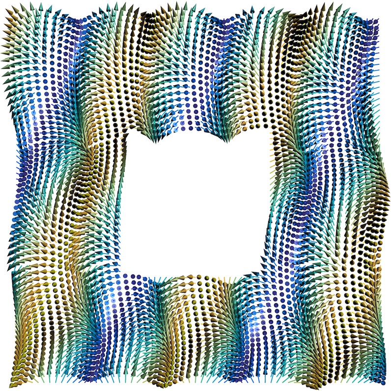
(a) Lossy Input data.

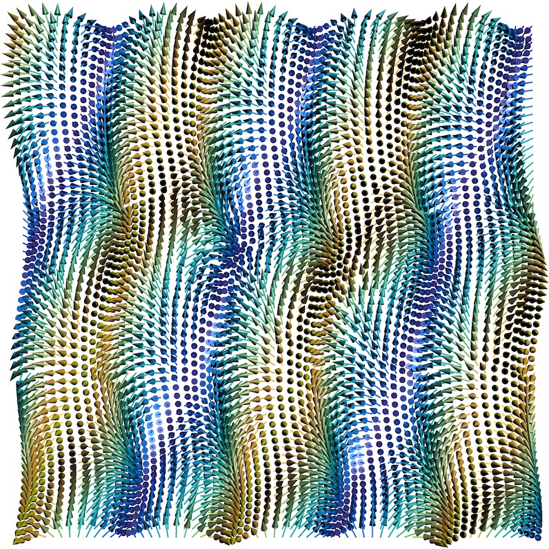
(b) Reconstruction,
$k=25$, $p=12$.

Figure 1: Reconstruction of directional data $f\in(\mathbb{S}^{2})^{64\times 64}$ from lossy given data, i. e.  in (1(a)) the original data is shown with missing data (the center). Using the $k=25$ most similar patches and a patch radius of $p=12$ leads to a reasonable reconstruction in (1(b)).

We investigate the presented algorithm for artificial manifold-valued data: first, let $\mathcal{M}=\mathbb{S}^{2}$ be the unit sphere, i.e., our data items are directions in $\mathbb{R}^{3}$. Its data items are drawn as small three-dimensional arrows color-encoded by elevation, i.e., the south pole is blue (dark), the north pole yellow (bright). The periodicity of the data is slightly obstructed by two vertical and horizontal discontinuities of jump height $\frac{\pi}{16}$ dividing the image into nine parts. The input data is given by the lossy data, cf. Fig. 1(a)). We set the search window to $r=32$, i.e., global comparison of patches in the graph construction from Sec. 4.1. Using $k=25$ most similar patches and a patch radius of $p=12$, the iterative scheme (7) yields Fig. 1(b)). The proposed methods finds a reasonable interpolation in the missing pixels.

4.3 Inpainting of symmetric positive definite matrices

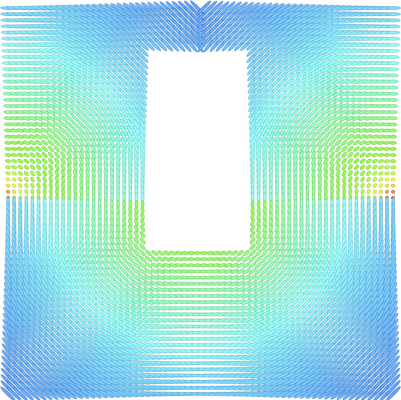
(a) Input data with missing rectangle.

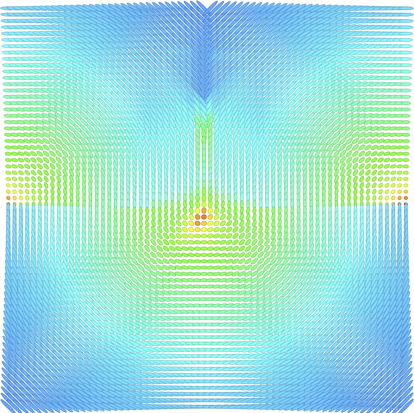
(b) Reconstruction, $k=5$, $p=6$.

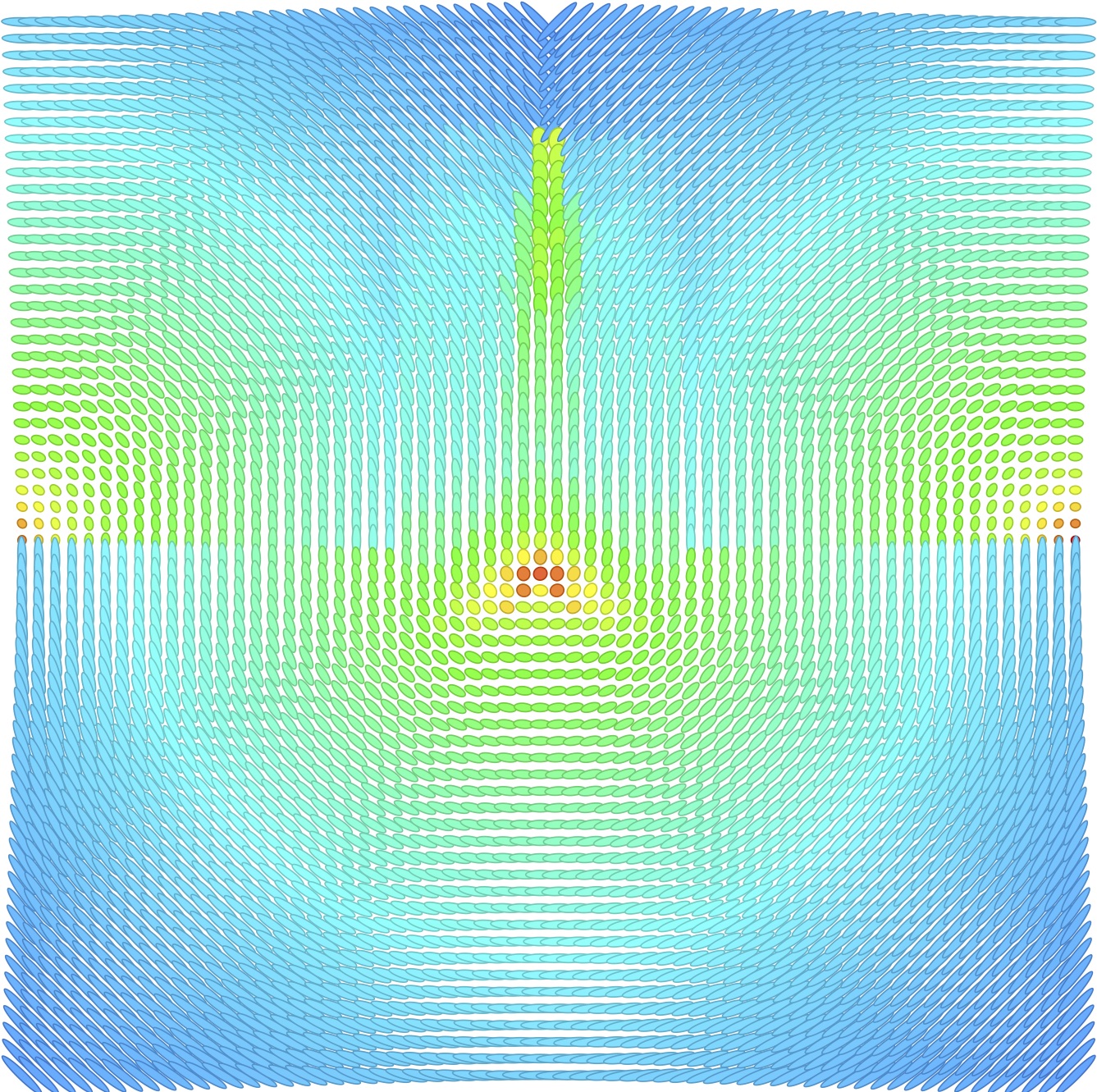
(c) Reconstruction, $k=25$, $p=6$.

Figure 2: Reconstruction of s.p.d. matrices $f\in(\mathcal{P}(2))^{64\times 64}$ of (2(a)) a lossy image. Increasing the number of neighbors from $k=5$ in (2(b)) to $k=25$ in (2(c)) broadens the center feature and smoothens the discontinuity in the center.

As a second example we consider an image of symmetric positive definite (s.p.d.) matrices from $\mathbb{R}^{2\times 2}$, i.e., $\mathcal{M}=\mathcal{P}(2)$. These can be illustrated as ellipses using their eigenvectors as main axes and their eigenvalues as their lengths and the geodesic anisotropy index [15] in the hue colormap. The input data of $64\times 64$ pixel is missing a rectangular area, cf. Fig. 2(a)). We set again $r=32$ for a global comparison. Choosing $k=5$, $p=6$ yields a first inpainting result shown in Fig. 2(b)) which preserves the discontinuity line in the center and introduces a red area within the center bottom circular structure. Increasing the nonlocal neighborhood to $k=25$, cf. in Fig. 2(c)) broadens the red center feature and the discontinuity gets smoothed along the center vertical line.

5 Conclusion

In this paper we introduced the graph $\infty$-Laplacian operator for manifold-valued functions by generalizing a reformulation of the $\infty$-Laplacian for real-valued functions and using discrete minimizing Lipschitz extensions. To the best of our knowledge, this generalization induced by our definition is even new for the vector-valued $\infty$-Laplacian on images. This case is included within this framework by setting e.g. $\mathcal{M}=\mathbb{R}^{3}$ for color images. We further derived an explicit numerical scheme to solve the related parabolic PDE on a finite weighted graph. First numerical examples using a nonlocal graph construction with patch-based similarity measures demonstrate the capabilities and performance of the inpainting algorithm applied to manifold-valued images.

Despite an analytic investigation of the convergence of the presented scheme, future work includes further development of numerical algorithms, as well as properties of the $\infty$-Laplacian for manifold-valued vertex functions on graphs.

References

- [1] P.-A. Absil, R. Mahony and R. Sepulchre “Optimization Algorithms on Matrix Manifolds” Princeton University Press: PrincetonOxford, 2008
- [2] M. Bačák, R. Bergmann, G. Steidl and A. Weinmann “A second order non-smooth variational model for restoring manifold-valued images” In SIAM J. Sci. Comput. 38.1, 2016, pp. A567–A597 DOI: 10.1137/15M101988X
- [3] P. Basser, J. Mattiello and D. LeBihan “MR diffusion tensor spectroscopy and imaging” In Biophys. J. 66 Elsevier, 1994, pp. 259–267 DOI: 10.1016/S0006-3495(94)80775-1
- [4] R. Bergmann, J. Persch and G. Steidl “A Parallel Douglas–Rachford Algorithm for Minimizing ROF-like Functionals on Images with Values in Symmetric Hadamard Manifolds” In SIAM J. Imaging Sci. 9.4, 2016, pp. 901–937 DOI: 10.1137/15M1052858
- [5] Ronny Bergmann and Daniel Tenbrinck “A Graph Framework for Manifold-valued Data” In arXiv preprint, 2017 URL: https://arxiv.org/abs/1702.05293
- [6] A. Buades, B. Coll and J.. Morel “A non-local algorithm for image denoising” In Proc. IEEE CVPR 2005 2, 2005, pp. 60–65 vol. 2 DOI: 10.1109/CVPR.2005.38
- [7] V. Caselles, J.-M. Morel and C. Sbert “An Axiomatic Approach to Image Interpolation” In Trans. Img. Proc. 7.3 IEEE Press, 1998, pp. 376–386 DOI: 10.1109/83.661188
- [8] M.G. Crandall, L.C. Evans and R.F. Gariepy “Optimal Lipschitz extensions and the infinity Laplacian” In Calc. Var. Partial Differ. Equ. 13.2, 2001, pp. 123–139 DOI: 10.1007/s005260000065
- [9] D. Cremers and E. Strekalovskiy “Total Cyclic Variation and Generalizations” In J. Math. Imaging Vis. 47.3, 2013, pp. 258–277 DOI: 10.1007/s10851-012-0396-1
- [10] A. Elmoataz, X. Desquesnes and O. Lezoray “Non-Local Morphological PDEs and p -Laplacian Equation on Graphs With Applications in Image Processing and Machine Learning” In IEEE J. Sel. Topics Signal Process. 6.7, 2012, pp. 764–779 DOI: 10.1109/JSTSP.2012.2216504
- [11] Jürgen Jost “Riemannian Geometry and Geometric Analysis” Springer-Verlang, Berlin Heidelberg, 2011 DOI: 10.1007/978-3-642-21298-7
- [12] J. Lellmann, E. Strekalovskiy, S. Koetter and D. Cremers “Total variation regularization for functions with values in a manifold” In Proc. IEEE ICCV 2013, 2013, pp. 2944–2951 DOI: 10.1109/ICCV.2013.366
- [13] Kantilal Varichand Mardia and Peter E. Jupp “Directional Statistics” Chichester: Wiley, 2000
- [14] D. Massonnet and K.. Feigl “Radar interferometry and its application to changes in the Earth’s surface” In Rev. Geophys. 36.4, 1998, pp. 441–500 DOI: 10.1029/97RG03139
- [15] Maher Moakher and Philipp G Batchelor “Symmetric Positive-Definite Matrices: From Geometry to Applications and Visualization” In Visualization and Processing of Tensor Fields Berlin: Springer, 2006, pp. 285–298 DOI: 10.1007/3-540-31272-2˙17
- [16] Adam M. Oberman “A convergent difference Scheme for the Infinity Laplacian: Construction of absolutely minimizing Lipschitz extensions” In Math. Comp. 74.251, 2004, pp. 1217–1230 DOI: 10.1090/S0025-5718-04-01688-6
- [17] Andreas Weinmann, Laurent Demaret and Martin Storath “Total variation regularization for manifold-valued data” In SIAM J. Imaging Sci. 7.4, 2014, pp. 2226–2257 DOI: 10.1137/130951075