Abstract. 

We compare quantum dynamics in the presence of Markovian dephasing for a particle hopping on a chain and for an Ising domain wall whose motion leaves behind a string of flipped spins. Exact solutions show that on an infinite chain, the transport responses of the models are nearly identical. However, on finite-length chains, the broadening of discrete spectral lines is much more noticeable in the case of a domain wall.

Introduction

The role of dephasing on the time evolution of a quantum mechanical system is a fundamental issue in the study of open quantum systems.

We pose the question what happens if the object moving around is not a simple pointlike particle, but rather an emergent quasiparticle which acts as a source of an observable emergent gauge field. One example is the monopole and Dirac string dynamics[1, 2] in spin ice[3]. As the full motion in a disordered spin background is beyond the scope of a first pass at this problem, we consider a simplified setting where the motion takes place in one dimension; we contrast the cases of a free particle and one with a string attached, in the form of a domain wall in an Ising system. Experimentally, this question corresponds, e.g., to the observation of a Villain mode in a quasi–one-dimensional magnet[4, 5].

Our central results are the following. The first is a technical one, namely that we can solve both cases (particle and domain wall motion) for a one-dimensional model subject to a locally uncorrelated Markovian dephasing bath. Secondly, this solution demonstrates that, for unstructured motion in one dimension, the two cases differ only weakly, in the sense that the difference between the two is considerably smaller than the difference between either and the fully coherent time evolution. In particular, linear transport responses in the presence of a linear density gradient or a uniform field are identical for the two cases. Thirdly, we notice that this is no longer the case when considering finite-length chains. Here, the discrete energy spectrum is broadened considerably more strongly for the case of domain walls; this can be qualitatively understood as the enhanced fragility of the interference of a domain wall with itself as it does a round trip on the finite lattice to establish the standing wave.

1 Models

The two models we solve both describe single-body one-dimensional hopping in the presence of Markovian dephasing uncorrelated between the sites, written in terms of the density matrix with components $\rho_{ab}$,

$$\dot{\rho}_{ab}=-i[H,\rho]_{ab}-\Gamma_{a-b}\,\rho_{ab},\quad(\mbox{\small\rm no summation!})$$ (1)

where dephasing rates for all off-diagonal elements of the density matrix are equal in the case of a particle (P), while they grow linearly with the distance from the diagonal in the case of a domain wall (DW),

$$\Gamma_{s}^{({\rm P})}=\gamma\,(1-\delta_{s,0}),\qquad\Gamma_{s}^{({\rm DW})}=\gamma\,|s|.$$ (2)

In Eq. (1), $H=H_{0}$ with the matrix elements

$$(H_{0})_{ab}=-{\Delta\over 2}(\delta_{a,b+1}+\delta_{a+1,b})$$ (3)

is the usual hopping Hamiltonian, $\delta_{a,b}$ is the Kronecker symbol, and the parameters $\Delta$ and $\gamma$ respectively denote the half band width and the dephasing rate.

Formally, Eqs. (1) with $\Gamma_{s}^{(\rm P)}$ of Eq. (2) can be considered a Lindblad equation[6] for particle hopping, where each site has its own bath coupled to its occupation number. It describes universal long-time dephasing physics valid in the limit where both the bath cutoff frequency $\omega_{c}$ (maximum frequency of a bath mode) and the bath temperature $\beta^{-1}$ are large compared to the hopping band width $2\Delta$.

Similarly, with $\Gamma_{s}^{(\rm DW)}$ of Eq. (2), these equations describe dynamics in a single-DW sector of an Ising spin chain in the presence of the transverse field $\Delta$, and independent fluctuating longitudinal magnetic fields. Moving the domain wall by $|a-b|$ positions requires flipping $|a-b|$ spins, which increases the dephasing rate for the matrix element $\rho_{ab}$.

2 Results

On an infinite chain, we use the translational symmetry and define the Fourier transformation for the center of mass,

$$\rho_{ab}=\int{dK\over 2\pi}e^{iKR}e^{i\pi s/2}\phi_{s}(K,t),\quad s\equiv a-b,$$ (4)

where $R\equiv(a+b)/2$ and the phase factor $e^{i\pi s/2}$ makes explicit the reflection symmetry, $s\to-s$. The densities $\phi_{s}(K,t)$ satisfy a 1D Schrödinger equation with hopping $u_{K}=\Delta\sin(K/2)$ and an imaginary on-site potential $-i\Gamma_{s}$.

(i) With $K=0$, densities $\phi_{s}(0,t)$ at different $s$ are independent from each other and, for $s\neq 0$, decay to zero with rates $\Gamma_{s}$. It is also easy to see that stationary solutions of Eq. (1) with the diagonal density $n_{s}\equiv\rho_{ss}$ in the form of a polynomial of degree $\ell\geq 0$ have all off-diagonal matrix elements with $|a-b|>\ell$ zero. In particular, with $n_{s}$ linear, the stationary solution $\rho_{ab}$ is tri-diagonal, which makes the linear diffusive transport of particles and DWs identical.

(ii) We obtained explicit solutions for Laplace-transformed densities $\psi_{s}\equiv{\psi}_{s}(K,p)$, with the initial condition $\phi_{s}(K,t=0)=\delta_{s,0}$ of a classical purely-diagonal density matrix:

$$\quad\psi^{({\rm P})}_{s}={e^{-i|s|\pi/2}\bigl{[}y\bigl{(}{p+\gamma\over 2u_{K}}\bigr{)}\bigr{]}^{|s|}\over[(p+\gamma)^{2}+4u_{K}^{2}]^{1/2}-\gamma},\;\,y(t)\equiv(1+t^{2})^{1/2}-t,$$

$$\quad\psi_{s}^{({\rm DW})}=e^{-i|s|\pi/2}{I_{p/\gamma+|s|}(z)\over\gamma z\,I_{p/\gamma}^{\prime}(z)},\quad z\equiv 2u_{K}/\gamma,$$

where $I_{\nu}(z)$ is the modified Bessel function of the first kind, and $I_{\nu}^{\prime}(z)=I_{\nu+1}(z)+(\nu/z)I_{\nu}(z)$ is its derivative. At $s=0$, these quantities are related to the dynamic structure factor $S(K,\omega)=\psi_{0}(K,\epsilon+i\omega)$, given by the spatial and temporal Fourier transform of the probability $P(s,t)$ to travel $s$ sites in time $t$. While functional forms differ for the two cases, plots of $S(K,\omega)$ at $\gamma/\Delta<1/10$ are remarkably similar (not shown due to space constraint). Also similar are the probabilities $P(s,t)$, see Fig. 1.

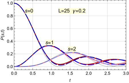
Fig. 1: Time dependence of the probabilities $P(s,t)$, $s=0,1,2$, for a particle (red solid lines) and for a DW (blue dashed lines) with $\Delta=2$ and dephasing $\gamma=0.2$. Thin black lines show the corresponding results at $\gamma=0$, $P(s,t)=J_{s}^{2}(\Delta\,t)$, where $J_{s}(z)$ is the Bessel function of order $s$. Even for such a relatively large $\gamma$, there is little difference between a particle and a DW.

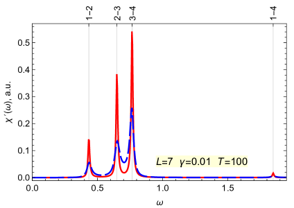
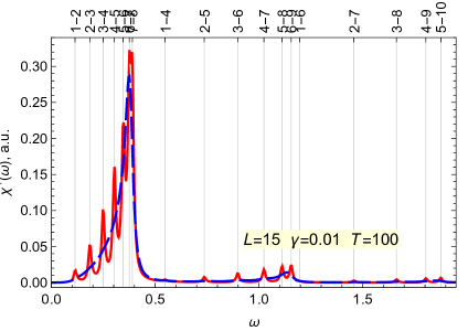
Fig. 2: Real part of the frequency-dependent susceptibility, $\chi^{\prime}(\omega)$, for a particle (red solid lines) and a DW (blue dashed lines) on chains of length $L=7$ and $L=15$ as indicated, with half band width $\Delta=2$ and dephasing $\gamma=0.01$. Vertical grid lines mark allowed transitions between the discrete energy levels in the absence of dephasing (only one level pair is shown for each line). While discrete lines for a particle are well resolved in both cases, they are suppressed entirely for a DW on the longer chain.

(iii) In spite of these similarities, finite-frequency responses on finite chains look different in the two cases. Indeed, a bound state is formed when a wave function interferes with itself; such an interference requires off-diagonal matrix elements of $\rho$. Solving linearized versions of Eqs. (1) with a harmonically modulated linear potential, and assuming the unperturbed thermal density matrix $e^{-\beta H_{0}}$, we analyzed the average conductance $\chi(\omega)$ [Fig. 2]. At small $\gamma$, the corresponding real part $\chi^{\prime}(\omega)$ has a series of resonant peaks at $\omega_{mn}=E_{m}-E_{n}$, where symmetry requires $m-n$ to be odd, and $E_{m}=-\Delta\cos k_{m}$, $k_{m}=\pi m/(L+1)$, are the energy levels of the chain (3) of length $L$, $m=1,2,\ldots,L$. In the case of a particle on such a chain, we find the width of each peak to be $\gamma(L-1)/(L+1)$, while for a DW on a chain with $L$ allowed positions, peak widths scale as $\gamma\,{\cal O}(L)$, as would be expected on general grounds.

3 Conclusions

Quantum mechanics teaches us that particles can behave as waves, and waves as particles. For weakly-interacting particles, this is described by second quantization. A superficially similar correspondence also exists outside of the perturbative sector where a topological defect can be often viewed as a particle, its motion described by the Schrödinger equation. Some of the examples are dislocations in lattices, vortices in 2D superfluids or superconductors, and various soliton-like defects in 1D systems. Experimentally observed quantum manifestations of such objects include position uncertainty and quantum delocalization of lattice defects, quantum tunneling of vortices and magnetic domain walls, and quantum transport in conducting polymers.

Our main conclusion is that this analogy between collective excitations and particles is not universal. Environment can severely limit the quantum behavior of such excitations.

Acknowledgements

This work was supported in part by the ARO grant W911NF-14-1-0272, the NSF grant PHY-1416578, and EPSRC grants EP/K028960/1 and EP/M007065/1.

References

- [1] L. D. C. Jaubert and P. C. W. Holdsworth, Nature Physics 5, 258 (2009).
- [2] Y. Wan and O. Tchernyshyov, Phys. Rev. Lett. 108, 247210 (2012), 1201.5314.
- [3] C. Castelnovo, R. Moessner, and S. Sondhi, Annual Review of Condensed Matter Physics 3(1), 35 (2012).
- [4] J. Villain, Physica B+C 79(1), 1 (1975).
- [5] S. E. Nagler, W. J. L. Buyers, R. L. Armstrong, and B. Briat, Phys. Rev. Lett. 49, 590 (1982).
- [6] G. Lindblad, Commun. Math. Phys. 48, 119 (1976).