Dissipation modulated Kelvin probe force microscopy method

Abstract

We review a new experimental implementation of Kelvin probe force microscopy (KPFM) in which the dissipation signal of frequency modulation atomic force microscopy (FM-AFM) is used for dc bias voltage feedback (D-KPFM). The dissipation arises from an oscillating electrostatic force that is coherent with the tip oscillation, which is caused by applying the ac voltage between the tip and sample. The magnitude of the externally induced dissipation is found to be proportional to the effective dc bias voltage, which is the difference between the applied dc voltage and the contact potential difference. Two different implementations of D-KPFM are presented. In the first implementation, the frequency of the applied ac voltage, $f_{\mathrm{el}}$, is chosen to be the same as the tip oscillation ($f_{\mathrm{el}}=f_{\mathrm{m}}$: $1\omega$D-KPFM). In the second one, the ac voltage frequency, $f_{\mathrm{el}}$, is chosen to be twice the tip oscillation frequency ($f_{\mathrm{el}}=2f_{\mathrm{m}}$: $2\omega$D-KPFM). In $1\omega$D-KPFM, the dissipation is proportional to the electrostatic force, which enables the use of a small ac voltage amplitude even down to $\approx 10$ mV. In $2\omega$D-KPFM, the dissipation is proportional to the electrostatic force gradient, which results in the same potential contrast as that obtained by FM-KPFM. D-KPFM features a simple implementation with no lock-in amplifier and faster scanning as it requires no low frequency modulation. The use of a small ac voltage amplitude in $1\omega$D-KPFM is of great importance in characterizing of technically relevant materials in which their electrical properties can be disturbed by the applied electric field. $2\omega$D-KPFM is useful when more accurate potential measurement is required. The operations in $1\omega$ and $2\omega$D-KPFM can be switched easily to take advantage of both features at the same location on a sample.

0.1 Introduction

Kelvin probe force microscopy (KPFM), a variant of atomic force microscopy (AFM) has become one of the indispensable tools used to investigate electronic properties of nanoscale material as well as nanoscale devices. In KPFM, a contact potential difference (CPD) between the AFM tip and sample surface is measured by detecting a capacitive electrostatic force, $F_{\mathrm{elec}}$, that is a function of the CPD, $V_{\mathrm{cpd}}$, and applied bias voltage, $V_{\mathrm{bias}}$ such as $F_{\mathrm{elec}}\propto(V_{\mathrm{bias}}-V_{\mathrm{cpd}})$. In order to separate the electrostatic force component from other force components such as van der Waals force, chemical bonding force and magnetic force, the capacitive electrostatic force is modulated by applying an ac voltage. and the resulting component of the measured observable, which are typically the resonant frequency shift or the change in amplitude of an oscillating AFM cantilever, is detected by lock-in detection Nonnenmacher91 .

KPFM has been implemented in a variety of ways that can be classified mostly into two distinct categories, amplitude modulation (AM-) KPFM  Nonnenmacher91 ; Kikukawa96 ; Sommerhalter1999 ; Zerweck05 and frequency modulation (FM-) KPFM Kitamura98 ; Zerweck05 .

In AM-KPFM, one of the cantilever resonance modes is excited by applying an ac voltage and the resulting oscillation amplitude is detected as a measure of the capacitive electrostatic force, which is used for controlling the dc bias voltage to nullify the oscillation amplitude. This implementations can take advantage of enhanced electrostatic force detection sensitivity by tuning the modulation frequency to one of the resonance frequencies of the AFM cantilever, leading to an enhanced detection of the electrostatic force by its quality ($Q$) factor that can reach over 10000 in vacuum environment Schumacher2015 . In single-pass implementation in which the topography and CPD images are taken simultaneously, the second flexural mode is usually chosen for detecting the electrostatic force while the first flexural mode is used for detecting short-range interaction which is used for the topography imaging.

In FM-KPFM, a low frequency (typically several hundred Hz) ac voltage is superposed with the dc bias voltage, resulting in the modulation in the resonance frequency shift. The amplitude of the modulated resonance frequency shift is detected by a lock-in amplifier and then used for the bias voltage feedback. Although this method requires a much higher ac voltage amplitude than AM-KPFM, it offers higher spatial resolution because the resonance frequency shift is determined by the electrostatic force gradient with respect to the tip-sample distance rather than the force itself Sommerhalter1999 ; Zerweck05 ; Burke09a .

In this chapter, we report two alternative KPFM implementations ($1\omega$D-KPFM and $2\omega$D-KPFM) in which the dissipation signal of a frequency modulation atomic force microscopy (FM-AFM) is used for detecting the capacitive electrostatic force Miyahara2015 ; Miyahara2017b . The dissipation is induced by applying a coherent sinusoidal ac voltage which is $90^{\circ}$ out of phase with respect to the tip oscillation. The externally induced dissipation signal can be used for the dc bias voltage feedback as it is proportional to the effective dc potential difference, $V_{\mathrm{dc}}\equiv(V_{\mathrm{bias}}-V_{\mathrm{cpd}})$.

In $1\omega$D-KPFM, the angular frequency of the applied ac voltage, $\omega_{\mathrm{el}}$, is chosen to be the same as the tip oscillation ($\omega_{\mathrm{el}}=\omega_{\mathrm{m}}$). In $2\omega$D-KPFM, $\omega_{\mathrm{el}}$ is chosen to be twice $\omega_{\mathrm{m}}$ ($\omega_{\mathrm{el}}=2\omega_{\mathrm{m}}$). We will show that, in $1\omega$D-KPFM, the induced dissipation is proportional to the electrostatic force, which enables the use of a small ac voltage amplitude down to $\approx 10$ mV whereas, in $2\omega$D-KPFM, the dissipation is proportional to the electrostatic force gradient, which results in the same potential contrast as that obtained by FM-KPFM.

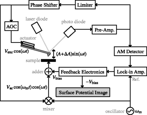
Figure 1: Block diagram of dissipation modulated Kelvin probe force microscopy technique proposed by Fukuma et al. Fukuma2004 . The induced dissipation is detected by measuring the change in the amplitude of tip oscillation. Reprinted from Fukuma2004 , with the permission of AIP Publishing

The idea of using induced dissipation for KPFM was first reported by Fukuma et al. Fukuma2004 which they named DM-KPFM. In their implementation, the dissipation is measured through the change in tip oscillation amplitude rather than the dissipation signal (Fig. 1). Despite the demonstrated higher sensitivity of DM-KPFM (Fig. 2), it has not been widely adopted, probably because of its rather complex implementation and limited detection bandwidth due to the amplitude detection Fukuma2004 . The use of the ac voltage with twice the frequency of the tip oscillation was proposed by Nomura et al. Nomura2007 for DM-KPFM to be sensitive to electrostatic force gradient rather than electrostatic force itself.

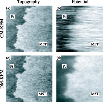
Figure 2: Topography and CPD images of dimethylquinquethiophene monolayer formed on a Pt surface. (a) topography and (b) CPD images taken by FM-KPFM. (c) topography and (d) CPD images taken by DM-KPFM. From Fukuma2004 . Reprinted from Fukuma2004 , with the permission of AIP Publishing

Our implementation of D-KPFM features a simple implementation with no lock-in amplifier enabling faster scanning as it requires no low frequency modulation. The use of a small ac voltage amplitude in $1\omega$D-KPFM is of great importance in characterizing technically relevant materials in which their electrical properties can be disturbed by the applied electric field (e.g. resulting in band-bending.effects at interfaces). $2\omega$D-KPFM is useful when more accurate potential measurement is required. The operations in $1\omega$ and $2\omega$D-KPFM can be switched easily to take advantage of both features at the same location on a sample.

0.2 Theory

In order to understand the operation principle of D-KPFM technique, we will first review the theory of FM-AFM and the effect of a periodic applied force on the in-phase and out-of-phase signal (commonly known as frequency shift and dissipation) of the FM-AFM system. We will then discuss the detailed analysis of the electrostatic force in the presence of the applied coherent ac voltage and how its effect appears in the resonant frequency shift and dissipation.

0.2.1 Review of theory of frequency modulation atomic force microscopy

Frequency shift and Dissipation in frequency modulation atomic force microscopy

We consider the following equation of motion of the AFM cantilever to model FM-AFM.

$$m\ddot{z}(t)+m\frac{\omega_{\mathrm{0}}}{Q}\dot{z}(t)+k\times(z(t)-z_{\mathrm{0}})=F_{\mathrm{ts}}(t)+F_{\mathrm{exc}}(t)$$ (1)

where $m$, $\omega_{\mathrm{0}}$, $Q$, $k$ are the effective mass and angular resonance frequency, mechanical quality factor and effective spring constant of the AFM cantilever. $z_{\mathrm{0}}$ is the mean distance of the tip measured from the sample surface. $F_{\mathrm{ts}}(t)$ and $F_{\mathrm{exc}}(t)$ are the force acting on the tip caused by tip-sample interaction and an external drive force that is used to excite the cantilever oscillation, respectively. In FM-AFM, the AFM cantilever is used as a mechanical resonator with a high $Q$ (typically $>1000$) which acts as a frequency determining component of a self-driven oscillator Albrecht1991 . Such a self-driven oscillator is realized by a positive feedback circuit equipped with an amplitude controller that keeps the oscillation amplitude constant Albrecht1991 ; Durig1997 . In this case, the external driving force, $F_{\mathrm{exc}}(t)$, is generated by a time-delayed (phase-shifted) cantilever deflection such as $F_{\mathrm{exc}}(t)=gkz(t-t_{0})$ which is commonly transduced by piezoacoustic or photothermal excitation scheme Labuda2012a through a phase shifter electronics. Here $g$ represents the gain of the positive feedback circuit and is called dissipation signal, and $t_{0}$ is the time delay set by the phase shifter . For the typical cantilever with a high $Q$ factor and high spring constant used for FM-AFM, we can assume a harmonic oscillation of the cantilever such as $z(t)=z_{0}+A\cos(\omega_{\mathrm{m}}t)$. When $t_{0}$ is set to be $\frac{1}{4}T_{0},\frac{3}{4}T_{0},\frac{5}{4}T_{0},\cdots$ ($T_{0}\equiv 2\pi/\omega_{\mathrm{0}}$), the oscillation frequency, $f_{\mathrm{m}}=\omega_{\mathrm{m}}/2\pi$, tracks its mechanical resonance frequency such that $f_{\mathrm{m}}=f_{0}(\equiv\omega_{\mathrm{0}}/2\pi)$. In this condition, the frequency shift, $\Delta f$, and dissipation signal, $g$, are expressed as follows Holscher2001 ; Kantorovich2004 ; Sader2005 :

$$\Delta f \approx -\frac{f_{0}^{2}}{kA}\int^{T_{0}}_{0}F_{\mathrm{ts}}(t)\cos(\omega_{\mathrm{m}}t)dt$$ (2)

$$g \approx \frac{1}{Q}+\frac{2f_{0}^{2}}{kA}\int^{T_{0}}_{0}F_{\mathrm{ts}}(t)\sin(\omega_{\mathrm{m}}t)dt.$$ (3)

It is important to notice that in general, the force acting on the tip, $F_{\mathrm{ts}}(t)$, can have an explicit time dependence in addition to the time dependence due to the time-varying tip position which is expressed as $F_{\mathrm{ts}}(z(t))$ Kantorovich2004 . The explicit time dependence can originate from various tip-induced processes such as dynamic structural relaxation of either tip or/and sample Kantorovich2004 and single-electron tunneling Miyahara2017 . In the case of electrostatic force, $F_{\mathrm{ts}}(t)$ is determined by the applied voltage as well as the tip position. It is thus essential to take into account both dependencies explicitly. Before going into further detail of the electrostatic force, we will look at the effect of time-varying periodic force on frequency shift and damping of the cantilever.

Effect of coherent periodic force on frequency shift and dissipation

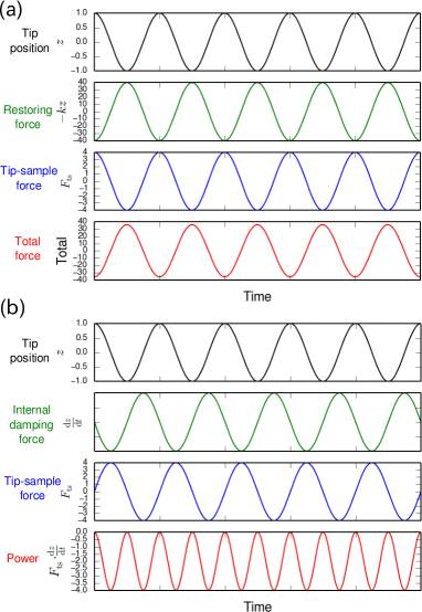
Figure 3: (a) Schematic representation of tip position, $z$, restoring force, $-kz$, the in-phase fundamental Fourier component, $F_{\mathrm{in}}\cos(\omega_{\mathrm{m}}t)$, and the total force. (b) Schematic representation of tip position, $z$, internal damping force, $m\gamma_{0}\dot{z}$, the quadrature fundamental Fourier component, $F_{\mathrm{quad}}\sin(\omega_{\mathrm{m}}t)$, and the instantaneous power delivered from the tip-sample interaction

In general, the periodically oscillating force, $F_{\mathrm{ts}}(t)$, can be represented by a Fourier series:

$$F_{\mathrm{ts}}(t)=F_{0}+\sum_{n=1}^{\infty}\{F_{\mathrm{in}}^{(n)}\cos(n\omega_{\mathrm{m}}t)+F_{\mathrm{quad}}^{(n)}\sin(n\omega_{\mathrm{m}}t)\}$$ (4)

The cosine terms represent the force component which is in phase (even) with the tip oscillation, which is conservative and the sine terms represent $90^{\circ}$ out-of-phase (quadrature, odd) component which is dissipative Sader2005 . Substituting Eq. 4 into Eq. 2 and 31 yields the following results :

$$\Delta f = -\frac{1}{2}\frac{f_{0}}{kA}F_{\mathrm{in}}^{(1)}$$ (5)

$$g = g_{0}\left(1+\frac{Q}{kA}F_{\mathrm{quad}}^{(1)}\right)$$ (6)

where $g_{0}\equiv 1/Q$ is the dissipation signal in the absence of $F_{\mathrm{ts}}(t)$, which is determined by the intrinsic damping of the cantilever. Eq. 5 and 6 indicate that $\Delta f$ and $g$ are proportional to the Fourier in-phase (even), $F_{\mathrm{in}}(\equiv F_{\mathrm{in}}^{(1)})$, and quadrature (odd), $F_{\mathrm{quad}}(\equiv F_{\mathrm{quad}}^{(1)})$, coefficients of the fundamental harmonic component (in this case $\omega_{\mathrm{m}}$) of $F_{\mathrm{ts}}(t)$, respectively. We can understand this results intuitively with the schematics shown in Fig. 3. Fig. 3(a) shows the tip position, $z$, restoring force, $-kz$, the in-phase fundamental Fourier component, $F_{\mathrm{in}}\cos(\omega_{\mathrm{m}}t)$, and the total force acting on the cantilever. Similarly, Fig. 3(b) shows the tip position, $z$, intrinsic damping force, $m\gamma_{0}\dot{z}$, the quadrature fundamental Fourier component, $F_{\mathrm{quad}}\sin(\omega_{\mathrm{m}}t)$, and the instantaneous power delivered from the tip-sample interaction. As can be seen from these figures, while the in-phase component just influences the restoring force, resulting in the resonance frequency shift, the quadrature component can change the damping force, resulting in a signal in the dissipation channel. This can also be understood by non-zero average power delivered by the quadrature tip-sample interaction as shown in the power-time plot (Fig. 3(b)).

0.2.2 Analysis of electrostatic force with ac bias voltage

The electrostatic force between two conductors connected to an ac and dc voltage source is described as follows:

$$F_{\mathrm{elec}}(t) = \frac{1}{2}\frac{\partial C}{\partial z}\{V_{\mathrm{bias}}+V_{\mathrm{ac}}\cos(\omega_{\mathrm{el}}t+\phi)-V_{\mathrm{cpd}}\}^{2}$$

$$= F_{\mathrm{dc}}+F_{\mathrm{\omega}}+F_{\mathrm{2\omega}}$$

$$F_{0} = \frac{1}{2}\frac{\partial C}{\partial z}\left[(V_{\mathrm{bias}}-V_{\mathrm{cpd}})^{2}+\frac{V_{\mathrm{ac}}^{2}}{2}\right]=\alpha\left(V_{\mathrm{dc}}^{2}+\frac{V_{\mathrm{ac}}^{2}}{2}\right)$$ (8)

$$F_{\mathrm{\omega}} = \frac{\partial C}{\partial z}(V_{\mathrm{bias}}-V_{\mathrm{cpd}})V_{\mathrm{ac}}\cos(\omega_{\mathrm{el}}t+\phi)$$ (9)

$$= 2\alpha V_{\mathrm{dc}}V_{\mathrm{ac}}\cos(\omega_{\mathrm{el}}t+\phi)$$

$$F_{\mathrm{2\omega}} = \frac{1}{4}\frac{\partial C}{\partial z}V_{\mathrm{ac}}^{2}\cos\{2(\omega_{\mathrm{el}}t+\phi)\}=\frac{1}{2}\alpha V_{\mathrm{ac}}^{2}\cos\{2(\omega_{\mathrm{el}}t+\phi)\}$$ (10)

where $C$ is the tip-sample capacitance, $V_{\mathrm{bias}}$ and $V_{\mathrm{cpd}}$ are the applied dc voltage and the contact potential difference (CPD), and $V_{\mathrm{ac}}$, $\omega_{\mathrm{el}}$, $\phi$ are the amplitude, angular frequency, and phase of the applied ac bias voltage. $V_{\mathrm{dc}}\equiv V_{\mathrm{bias}}-V_{\mathrm{cpd}}$ is the effective dc bias voltage. It is important to notice that although the three force component terms, $F_{0}$, $F_{\mathrm{\omega}}$, $F_{\mathrm{2\omega}}$, are grouped by the frequency of $\omega_{\mathrm{el}}$ harmonic component such as 0, $\omega$, $2\omega$, they do not represent the frequency of harmonic components of the actual oscillating electrostatic force in the presence of the mechanical tip oscillation because $\displaystyle\alpha\equiv\frac{1}{2}\frac{\partial C}{\partial z}(z(t))$ is also a function of time through the time-dependent tip position $z(t)=z_{0}+A\cos(\omega_{\mathrm{m}}t)$. It is the interaction of the oscillating electric field and mechanical tip oscillation that results in an “electro-mechanical heterodyning” effect as we will see below.

By Taylor expanding $\alpha(z)$ around the mean tip position $z_{0}$,

$$\alpha(z) = \alpha(z_{0})+\alpha^{\prime}(z-z_{0})+\frac{1}{2}\alpha^{\prime\prime}(z-z_{0})^{2}+....$$ (11)

$$= \alpha_{0}+\alpha^{\prime}A\cos(\omega_{\mathrm{m}}t)+\frac{1}{2}\alpha^{\prime\prime}A^{2}\cos^{2}(\omega_{\mathrm{m}}t)+....$$

Taking the first order yields,

$$\alpha(z)\approx\alpha_{0}+\alpha^{\prime}(z-z_{0})=\alpha_{0}+\alpha^{\prime}A\cos(\omega_{\mathrm{m}}t).$$ (12)

Substituting $\alpha(z)$ into Eq. 8 yields

$$F_{0}(t) = \{\alpha_{0}+\alpha^{\prime}A\cos(\omega_{\mathrm{m}}t)\}\left(V_{\mathrm{dc}}^{2}+\frac{V_{\mathrm{ac}}^{2}}{2}\right)$$ (13)

$$= \alpha_{0}\left(V_{\mathrm{dc}}^{2}+\frac{V_{\mathrm{ac}}^{2}}{2}\right)+\alpha^{\prime}A\left(V_{\mathrm{dc}}^{2}+\frac{V_{\mathrm{ac}}^{2}}{2}\right)\cos(\omega_{\mathrm{m}}t).$$

The first term in Eq. 13 represents a time-invariant force which causes the static deflection of the cantilever whereas the second term represents an oscillating force with frequency of $\omega_{\mathrm{m}}/2\pi$. As this oscillating force is in phase with $z(t)$, it causes the shift in the resonance frequency.

Next, we look at $F_{\mathrm{\omega}}$ and $F_{\mathrm{2\omega}}$ terms (Eq. 9 and 10) in the same way:

$$\begin{split}F_{\mathrm{\omega}}(t)&=2\{\alpha_{0}+\alpha^{\prime}A\cos(\omega_{\mathrm{m}}t)\}V_{\mathrm{dc}}V_{\mathrm{ac}}\cos(\omega_{\mathrm{el}}t+\phi)\\ &=2\alpha_{0}V_{\mathrm{dc}}V_{\mathrm{ac}}\{\cos(\omega_{\mathrm{el}}t)\cos\phi-\sin(\omega_{\mathrm{el}}t)\sin\phi\}\\ &+\alpha^{\prime}AV_{\mathrm{dc}}V_{\mathrm{ac}}[\cos\{(\omega_{\mathrm{el}}+\omega_{\mathrm{m}})t+\phi\}+\cos\{(\omega_{\mathrm{el}}-\omega_{\mathrm{m}})t+\phi\}]\end{split}$$ (14)

$$\begin{split}F_{\mathrm{2\omega}}(t)&=\frac{1}{2}\{\alpha_{0}+\alpha^{\prime}A\cos(\omega_{\mathrm{m}}t)\}V_{\mathrm{ac}}^{2}\cos\{2(\omega_{\mathrm{el}}t+\phi)\}\\ &=\frac{1}{2}\alpha_{0}V_{\mathrm{ac}}^{2}\cos\{2(\omega_{\mathrm{el}}t+\phi)\}\\ &+\frac{1}{4}\alpha^{\prime}AV_{\mathrm{ac}}^{2}[\cos\{(2\omega_{\mathrm{el}}-\omega_{\mathrm{m}})t+2\phi\}+\cos\{(2\omega_{\mathrm{el}}+\omega_{\mathrm{m}})t+2\phi\}].\end{split}$$ (15)

Here, we notice that the electro-mechanical heterodyning produces other spectral components ($\omega_{\mathrm{el}}+\omega_{\mathrm{m}}$, $\omega_{\mathrm{el}}-\omega_{\mathrm{m}}$, $2\omega_{\mathrm{el}}-\omega_{\mathrm{m}}$, $2\omega_{\mathrm{el}}+\omega_{\mathrm{m}}$) than $\omega_{\mathrm{el}}$ and $2\omega_{\mathrm{el}}$ which are usually considered in the most KPFM literature. In order to calculate the frequency shift and damping, these additional spectral components need to be included. In the following, we consider two interesting cases (1) $\omega_{\mathrm{el}}=\omega_{\mathrm{m}}$, and (2) $\omega_{\mathrm{el}}=2\omega_{\mathrm{m}}$ which corresponds to $1\omega$D-KPFM and $2\omega$D-KPFM, respectively.

Case I , $\omega_{\mathrm{el}}=\omega_{\mathrm{m}}$: $1\omega$D-KPFM

In the case of $\omega_{\mathrm{el}}=\omega_{\mathrm{m}}$, gathering the time invariant terms found in $F_{0}$ (Eq. 13) and $F_{\mathrm{\omega}}$ (Eq. 14), the actual dc term, $F_{\mathrm{dc}}(t)$ can be found to be:

$$F_{\mathrm{dc}}^{1\omega}(t) = \alpha_{0}\left(V_{\mathrm{dc}}^{2}+\frac{V_{\mathrm{ac}}^{2}}{2}\right)+\alpha^{\prime}AV_{\mathrm{dc}}V_{\mathrm{ac}}\cos\phi.$$ (16)

The terms with $\omega_{\mathrm{m}}$ are found in $F_{0}$ (Eq. 13), $F_{\mathrm{\omega}}$ (Eq. 14) and $F_{\mathrm{2\omega}}$ (Eq. 15) and gathering them yields the following result:

$$\begin{split}F_{\omega_{\mathrm{m}}}^{1\omega}(t)&=2\alpha_{0}V_{\mathrm{dc}}V_{\mathrm{ac}}\cos(\omega_{\mathrm{m}}t+\phi)\\ &\quad+\alpha^{\prime}A\left\{\left(V_{\mathrm{dc}}^{2}+\frac{V_{\mathrm{ac}}^{2}}{2}\right)\cos(\omega_{\mathrm{m}}t)+\frac{1}{4}V_{\mathrm{ac}}^{2}\cos(\omega_{\mathrm{m}}t+2\phi)\right\}\\ &=2\alpha_{0}V_{\mathrm{dc}}V_{\mathrm{ac}}\{\cos(\omega_{\mathrm{m}}t)\cos\phi-\sin(\omega_{\mathrm{m}}t)\sin\phi\}\\ &\quad+\alpha^{\prime}A\left(V_{\mathrm{dc}}^{2}+\frac{V_{\mathrm{ac}}^{2}}{2}\right)\cos(\omega_{\mathrm{m}}t)\\ &\quad+\frac{1}{4}\alpha^{\prime}AV_{\mathrm{ac}}^{2}\{\cos(\omega_{\mathrm{m}}t)\cos(2\phi)-\sin(\omega_{\mathrm{m}}t)\sin(2\phi)\}\\ &=\left\{\alpha^{\prime}AV_{\mathrm{dc}}^{2}+2\alpha_{0}V_{\mathrm{dc}}V_{\mathrm{ac}}\cos\phi+\frac{\alpha^{\prime}A}{2}\left(1+\frac{1}{2}\cos(2\phi)\right)V_{\mathrm{ac}}^{2}\right\}\cos(\omega_{\mathrm{m}}t)\\ &\quad-2V_{\mathrm{ac}}\left\{\alpha_{0}V_{\mathrm{dc}}\sin\phi+\frac{1}{4}\alpha^{\prime}AV_{\mathrm{ac}}\sin(2\phi)\right\}\sin(\omega_{\mathrm{m}}t)\\ &=F_{\mathrm{in}}^{1\omega}\cos(\omega_{\mathrm{m}}t)+F_{\mathrm{quad}}^{1\omega}\sin(\omega_{\mathrm{m}}t)\end{split}$$ (17)

As we have seen in Sect. 0.2.1, the amplitude of $\cos(\omega_{\mathrm{m}}t)$ and $\sin(\omega_{\mathrm{m}}t)$ terms, $F_{\mathrm{in}}^{1\omega}$ and $F_{\mathrm{quad}}^{1\omega}$, determine the frequency shift, $\Delta f$, and dissipation, $g$, respectively. Here the superscript, $1\omega$, refers to the case of $\omega_{\mathrm{el}}=\omega_{\mathrm{m}}$ and thus $1\omega$D-KPFM.

$F_{\mathrm{in}}^{1\omega}$ and $F_{\mathrm{quad}}^{1\omega}$ are expressed as follows:

$$\begin{split}F_{\mathrm{in}}^{1\omega}&=\alpha^{\prime}AV_{\mathrm{dc}}^{2}+2\alpha_{0}V_{\mathrm{dc}}V_{\mathrm{ac}}\cos\phi+\frac{\alpha^{\prime}A}{2}\left(1+\frac{\cos(2\phi)}{2}\right)V_{\mathrm{ac}}^{2}\\ &=\alpha^{\prime}A\left(V_{\mathrm{dc}}+\frac{\alpha_{0}\cos\phi}{\alpha^{\prime}A}V_{\mathrm{ac}}\right)^{2}-\left[\frac{\alpha_{0}^{2}\cos^{2}\phi}{\alpha^{\prime}A}-\frac{\alpha^{\prime}A}{2}\left(1+\frac{\cos(2\phi)}{2}\right)\right]V_{\mathrm{ac}}^{2}\end{split}$$ (18)

$$\begin{split}F_{\mathrm{quad}}^{1\omega}&=-2V_{\mathrm{ac}}\left\{\alpha_{0}V_{\mathrm{dc}}\sin\phi+\frac{1}{4}\alpha^{\prime}AV_{\mathrm{ac}}\sin(2\phi)\right\}\\ &=-2\alpha_{0}V_{\mathrm{ac}}\sin\phi\left(V_{\mathrm{dc}}+\frac{1}{2}\frac{\alpha^{\prime}A\cos\phi}{\alpha_{0}}V_{\mathrm{ac}}\right)\end{split}$$ (19)

Eq. 18 shows that $\Delta f$ - $V_{\mathrm{bias}}$ curve is a parabola whose minima is located at by $\displaystyle V_{\mathrm{bias}}=V_{\mathrm{cpd}}-\frac{\alpha_{0}}{\alpha^{\prime}A}V_{\mathrm{ac}}\cos\phi$ and $g$ - $V_{\mathrm{bias}}$ curve is a straight line which intersects $F_{\mathrm{quad}}=0$ line at $\displaystyle V_{\mathrm{bias}}=V_{\mathrm{cpd}}-\frac{1}{2}\frac{\alpha^{\prime}A}{\alpha_{0}}V_{\mathrm{ac}}\cos\phi$.

When $\phi=90$ is chosen, we find

$$F_{\mathrm{in}}^{1\omega}=\alpha^{\prime}A\left(V_{\mathrm{dc}}^{2}+\frac{V_{\mathrm{ac}}^{2}}{4}\right)$$ (20)

$$F_{\mathrm{quad}}^{1\omega}=-2\alpha_{0}(V_{\mathrm{bias}}-V_{\mathrm{cpd}})V_{\mathrm{ac}}$$ (21)

Substituting Eq. 20 and 21 into Eq. 5 and 6 yields

$$\Delta f =-\frac{1}{2}\frac{f_{0}}{k}\frac{F_{\mathrm{in}}}{A}=-\frac{1}{2}\frac{f_{0}}{k}\alpha^{\prime}\left\{(V_{\mathrm{bias}}-V_{\mathrm{cpd}})^{2}+\frac{V_{\mathrm{ac}}^{2}}{4}\right\}$$ (22)

$$g =g_{0}\left(1-\frac{Q}{kA}F_{\mathrm{quad}}\right)=g_{0}\left\{1+2\frac{Q}{kA}\alpha_{0}(V_{\mathrm{bias}}-V_{\mathrm{cpd}})V_{\mathrm{ac}}\right\}$$ (23)

In this case, the dissipation, $g$, is proportional to $V_{\mathrm{dc}}=V_{\mathrm{bias}}-V_{\mathrm{cpd}}$. It is therefore possible to use the dissipation signal, $g$, as the KPFM bias voltage feedback signal with $g_{0}$ as its control setpoint value. It is important to notice that $\Delta f$ is proportional to electrostatic force gradient whereas $g$ is proportional to electrostatic force.

Case II , $\omega_{\mathrm{el}}=2\omega_{\mathrm{m}}$: $2\omega$D-KPFM

In this case, $\omega_{\mathrm{el}}+\omega_{\mathrm{m}}=3\omega_{\mathrm{m}}$ and $\omega_{\mathrm{el}}-\omega_{\mathrm{m}}=\omega_{\mathrm{m}}$. The actual dc term, $F_{\mathrm{dc}}$, becomes:

$$F_{\mathrm{dc}}^{2\omega}(t)=\alpha_{0}\left(V_{\mathrm{dc}}^{2}+\frac{V_{\mathrm{ac}}^{2}}{2}\right)$$ (24)

The terms with $\omega_{\mathrm{m}}$ are found in $F_{0}$ (Eq. 13), $F_{\mathrm{\omega}}$ (Eq. 14) in this case and results in

$$\begin{split}F_{\omega_{\mathrm{m}}}^{2\omega}(t)&=\alpha^{\prime}A\left\{\left(V_{\mathrm{dc}}^{2}+\frac{V_{\mathrm{ac}}^{2}}{2}\right)\cos(\omega_{\mathrm{m}}t)+V_{\mathrm{dc}}V_{\mathrm{ac}}\cos(\omega_{\mathrm{m}}t+\phi)\right\}\\ &=\left\{V_{\mathrm{dc}}^{2}+V_{\mathrm{dc}}V_{\mathrm{ac}}\cos\phi+\frac{V_{\mathrm{ac}}^{2}}{2}\right\}\cos(\omega_{\mathrm{m}}t)\\ &\quad-\alpha^{\prime}AV_{\mathrm{dc}}V_{\mathrm{ac}}\sin\phi\sin(\omega_{\mathrm{m}}t)\\ &=F_{\mathrm{in}}^{2\omega}\cos(\omega_{\mathrm{m}}t)+F_{\mathrm{quad}}^{2\omega}\sin(\omega_{\mathrm{m}}t)\end{split}$$ (25)

where

$$F_{\mathrm{in}}^{2\omega} =\alpha^{\prime}A\left(V_{\mathrm{dc}}+\frac{V_{\mathrm{ac}}}{2}\cos\phi\right)^{2}+\frac{\alpha^{\prime}A}{2}\left(1-\frac{\cos^{2}\phi}{2}\right)V_{\mathrm{ac}}^{2}$$ (26)

$$F_{\mathrm{quad}}^{2\omega} =-\alpha^{\prime}AV_{\mathrm{dc}}V_{\mathrm{ac}}\sin\phi$$ (27)

When $\phi=90^{\circ}$,

$$F_{\mathrm{in}}^{2\omega} =\alpha^{\prime}A\left(V_{\mathrm{dc}}^{2}+\frac{V_{\mathrm{ac}}^{2}}{2}\right)$$ (28)

$$F_{\mathrm{quad}}^{2\omega} =-\alpha^{\prime}AV_{\mathrm{dc}}V_{\mathrm{ac}}$$ (29)

In contrast to $\omega_{\mathrm{el}}=\omega_{\mathrm{m}}$ case (Eq. 19), $F_{\mathrm{quad}}$ is proportional to $\alpha^{\prime}$ rather than $\alpha$, indicating $g$ is sensitive to electrostatic force gradient. Substituting Eqs. 28 and 29 into Eqs. 5 and 6 yields:

$$\Delta f =-\frac{1}{2}\frac{f_{0}}{k}\frac{F_{\mathrm{in}}}{A}=-\frac{1}{2}\frac{f_{0}}{k}\alpha^{\prime}\left\{(V_{\mathrm{bias}}-V_{\mathrm{cpd}})^{2}+\frac{V_{\mathrm{ac}}^{2}}{2}\right\}$$ (30)

$$g =g_{0}\left(1-\frac{Q}{kA}F_{\mathrm{quad}}\right)=g_{0}\left\{1+\frac{Q}{k}\alpha^{\prime}(V_{\mathrm{bias}}-V_{\mathrm{cpd}})V_{\mathrm{ac}}\right\}.$$ (31)

Here we notice the following two important points: (1) the apparent shift of $V_{\mathrm{cpd}}$ appearing in $\Delta f$-$V_{\mathrm{bias}}$ curve does not depend on $\alpha$ and is just determined by $\phi$ and $V_{\mathrm{ac}}$, (2) there is no apparent shift of $V_{\mathrm{cpd}}$ in a $g$-$V_{\mathrm{bias}}$ curve. The point (2) indicates an important advantage of $2\omega$D-KPFM over $1\omega$D-KPFM as there is no need for carefully adjusting the phase, $\phi$, for accurate $V_{\mathrm{cpd}}$ measurements.

0.3 Experimental

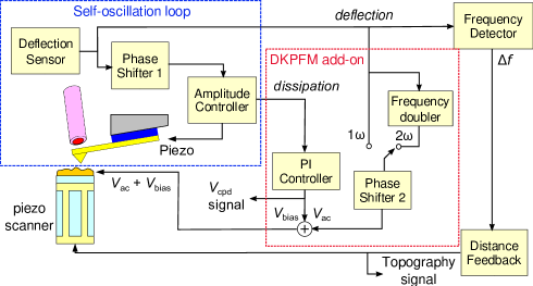
Figure 4: Block diagram of the experimental setup for force sensitive ($1\omega$D-KPFM) and force-gradient sensitive ($2\omega$D-KPFM) dissipation modulated KPFM techniques. Reprinted from Miyahara2017b , with the permission of AIP Publishing

Figure 4 depicts the block diagram of the experimental setup used for both $1\omega$ and $2\omega$D-KPFM measurements. The setup is based on the self-oscillation mode FM-AFM system  Albrecht1991 . While two additional components, a phase shifter, a proportional-integrator (PI) controller, are required for both $1\omega$ and $2\omega$D-KPFM operation, a frequency doubler that generates an ac voltage with the frequency of $2\omega_{\mathrm{m}}$ from the cantilever deflection signal is also required for $2\omega$D-KPFM operation. The amplitude controller that consists of a root-mean-square (RMS) amplitude detector and a PI controller (NanoSurf easyPLLplus oscillator controller) is used to keep the amplitude of tip oscillation constant. The detection bandwidth of the RMS amplitude detector is extended to about 3 kHz by replacing the integration capacitor in the original RMS detector circuit. The output of the amplitude controller is the dissipation signal.

The cantilever deflection signal is fed into the additional phase shifter (Phase shifter 2), which serves to adjust the relative phase, $\phi$, to produce the coherent ac voltage that is 90^∘ out of phase with respect to the cantilever deflection oscillation. The frequency doubler is used to produce a sinusoidal ac voltage with two times the tip oscillation frequency. The dissipation signal acts as the input signal to the PI controller, which adjusts $V_{\mathrm{bias}}$ to maintain a constant dissipation equal to the value without $V_{\mathrm{ac}}$ applied, $g_{0}$. Although in the following experiments we used a digital lock-in amplifier (HF2LI, Zurich Instruments) operated in the external reference mode as a phase shifter as well as a frequency doubler for convenience, other simpler phase shifter circuits such an all-pass filter can also be used for the D-KPFM measurements.

We used a JEOL JSPM-5200 atomic force microscope for the experiments with the modifications described below. The original laser diode was replaced by a fiber-optic collimator with a focusing lens that is connected to a fiber-coupled laser diode module (OZ Optics). The laser diode was mounted on a temperature controlled fixture and its driving current was modulated with a radio frequency signal with a RF bias-T (Mini-Circuits: PBTC-1GW). to reduce the deflection detection noise Fukuma05 . The deflection noise density floor as low as 13 fm$/\sqrt{\text{Hz}}$ was achieved. An open source scanning probe microscopy control software GXSM was used for the control and data acquisition Zahl2010 . A commercial silicon AFM cantilever (NSC15, MikroMasch) with a typical spring constant of about 20 N/m and resonance frequency of $\sim 300$ kHz was used in high-vacuum environment with the pressure of $1\times 10^{-7}$ mbar. The ac and dc voltages was applied to the sample with respect to the grounded tip to minimize the capacitive crosstalk Diesinger2008 to the piezoelectric plate used for driving cantilever oscillation that is located beneath the cantilever support.

0.4 Results and discussion

0.4.1 Validation of D-KPFM theory

In order to validate the analysis described in the previous sections  0.2.2 and 0.2.2, $\Delta f$-$V_{\mathrm{bias}}$ and $g$-$V_{\mathrm{bias}}$ curves are measured with the coherent ac voltage with different phases applied.

$1\omega$D-KPFM case

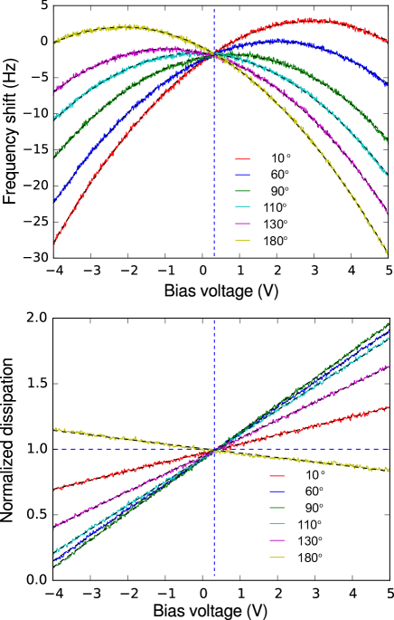
Figure 5: Validation of $1\omega$D-KPFM theory. (a) Frequency shift, $\Delta f$, and (b) dissipation signal, $g$, versus dc bias voltage, $V_{\mathrm{bias}}$, curves taken with a coherent sinusoidally oscillating voltage with the amplitude, $V_{\mathrm{ac}}=100$ mV_p-p and various phases, $\phi$, applied to a 200 nm thick SiO₂ on Si substrate. The dissipation signal is normalized with the value without the ac bias voltage (indicated with the horizontal blue dashed line). In both figures, each of dashed lines represent fitted curves assuming a parabola for $\Delta f$ and a linear line for $g$ as indicated in Eq. 18 and 19, respectively. The oscillation amplitude of the tip was 7.2 nm_p-p and the quality factor of the cantilever was 9046. Reprinted with permission from Miyahara2015 . Copyright 2016 by the American Physical Society

.

Figure 5 shows simultaneously measured $\Delta f$ and $g$ versus $V_{\mathrm{bias}}$ curves with a coherent sinusoidally oscillating voltage with the amplitude, $V_{\mathrm{ac}}=100$ mV_p-p and various phase, $\phi$. The curves were taken on a Si substrate with 200 nm thick oxide SiO₂. A fitted curve with a parabola for $\Delta f$-$V_{\mathrm{bias}}$ curves (Eq. 18) or a linear line for $g$-$V_{\mathrm{bias}}$ curves (Eq. 19) is overlaid on each experimental curve, indicating a very good agreement between the theory and experiments. As can be seen in Fig. 5(a) and (b), the position of the parabola vertex shifts and the slope of $g$-$V_{\mathrm{bias}}$ curve changes systematically with varying phase.

In order to further validate the theoretical analysis, the voltage coordinate for the vertices (parabola maximum) of $\Delta f$-$V_{\mathrm{bias}}$ curves and the slope of $g$-$V_{\mathrm{bias}}$ lines (dissipation slope) are plotted against the phase, $\phi$, in Fig. 6. Each plot is overlaid with a fitted curve (solid curve) with the cosine function (Eq. 18) for the parabola maximum and with the sine function (Eq. 19) for the dissipation slope, demonstrating an excellent agreement between the experiment and theory. The parabola maximum versus phase curve intersects that for the parabola without ac voltage at the phase of 97^∘ as opposed to 90^∘ which is predicted by the theory. This deviation is mainly due to the phase delay in the photodiode preamplifer electronics. The dissipation slope takes its maximum value at around 81^∘, again deviating from the theoretical value of 90^∘. This deviation is probably due to the residual capacitive crosstalk to the excitation piezo Diesinger2008 ; Melin2011 .

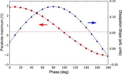
Figure 6: Parabola maximum of the measured $\Delta f$-$V_{\mathrm{bias}}$ curves (red circles) (Fig. 5(a)) and the dissipation slope of $g$-$V_{\mathrm{bias}}$ curves (blue circles) (Fig. 5(b)). Each solid line represents the fitted curve with the cosine function (Eq. 18) for the parabola minimum and with the sine function (Eq. 19) for the dissipation slope. The horizontal dashed line indicates the voltage for parabola maximum without the ac bias voltage. Reprinted with permission from Miyahara2015 . Copyright 2016 by the American Physical Society

$2\omega$D-KPFM case

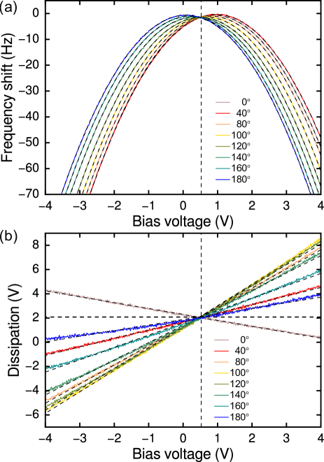
Figure 7: (a) Frequency shift, $\Delta f$, and (b) dissipation signal, $g$, versus dc bias voltage, $V_{\mathrm{bias}}$, curves taken with a coherent sinusoidally oscillating voltage with $\omega_{\mathrm{el}}=2\omega_{\mathrm{m}}$, $V_{\mathrm{ac}}=1$ V and various $\phi$, applied to a template stripped gold substrate. The vertical dashed line in (a) and (b) indicates $V_{\mathrm{cpd}}$ which is measured as the voltage coordinate of the parabola vertex without $V_{\mathrm{ac}}$. The horizontal dashed line in (b) indicates the dissipation without $V_{\mathrm{ac}}$. In both figures, each of dashed lines represent fitted curves assuming a parabola for $\Delta f$ and a linear line for $g$ as indicated in Eqs. 26 and 27, respectively. The oscillation amplitude of the tip was 10 nm_p-p and the quality factor of the cantilever was 25000

In order to validate Eqs. 26 and 27, $\Delta f$-$V_{\mathrm{bias}}$ and $g$-$V_{\mathrm{bias}}$ curves were measured while a coherent sinusoidally oscillating voltage with $\omega_{\mathrm{el}}=2\omega_{\mathrm{m}}$, $V_{\mathrm{ac}}=1$ V (2 V${}_{\mathrm{p-p}})$ and various phases, $\phi$, is superposed with $V_{\mathrm{bias}}$.

Figure 7(a) and (b) show the simultaneously measured $\Delta f$ and $g$ versus $V_{\mathrm{bias}}$ curves, respectively. The curves are taken on a template stripped gold surface. A fitted curve with a parabola for each of the $\Delta f$-$V_{\mathrm{bias}}$ curves (Eq. 26) or with a linear line for each of the $g$-$V_{\mathrm{bias}}$ curves (Eq. 27) is overlaid on each experimental curve, indicating a very good agreement between the theory and experiments. As can be seen in Fig. 7(a) and (b), the position of the parabola vertex shifts both in $V_{\mathrm{bias}}$ and $\Delta f$ axes and the slope of $g$-$V_{\mathrm{bias}}$ curve changes systematically with the varied phase, $\phi$. For further validating the theory, the voltage coordinate of the parabola vertex (parabola maximum voltage) of each $\Delta f$-$V_{\mathrm{bias}}$ curve and the slope of each $g$-$V_{\mathrm{bias}}$ curve are plotted against $\phi$ in Fig. 8. Each plot is overlaid with a fitted curve (solid curve) with the cosine function (see Eq. 26) for the parabola minimum voltage and with the sine function (Eq. 27) for the dissipation slope, demonstrating an excellent agreement between the experiment and theory. The $V_{\mathrm{bias}}$ dependence of the frequency shift coordinate of the parabola vertices (frequency shift offset) also shows a very good agreement with the theory (second term of Eq. 26) as shown in Fig. 8(b). The parabola minimum voltage versus phase curve intersects that of $\Delta f$-$V_{\mathrm{bias}}$ without ac bias voltage at $\phi=121^{\circ}$. The deviation from the theoretically predicted value of 90^∘ is due to the phase delay in the detection electronics. We also notice that the amplitude of parabola minimum versus phase curve is 0.472 V which is in good agreement with 0.5 V predicted by the theory ($V_{\mathrm{ac}}/2$ in Eq. 26).

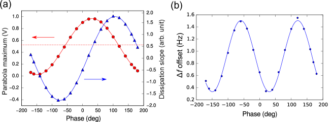
Figure 8: (a) Voltage coordinate of the vertices of the measured $\Delta f$-$V_{\mathrm{bias}}$ curves (parabola maximum) (red circles) extracted from the results Fig. 7(a) and the slope of dissipation-$V_{\mathrm{bias}}$ curves (blue triangles) extracted from Fig. 7(b) as a function of phase. Each solid line represents the fitted curve with the cosine function (Eq. 26) for the parabola maximum and with the sine function (Eq. 27) for the dissipation slope. The horizontal dashed line indicates the voltage coordinate of the parabola measured without the ac bias voltage. (b) $\Delta f$ offset as a function of phase. The solid line represents the fitted curve with the second term of Eq. 26. Reprinted from Miyahara2017b , with the permission of AIP Publishing

0.4.2 Illustrative example of D-KPFM imaging

Fig. 9 shows an example to illustrate how this technique works. Fig. 9(a) and (b) show the topography and dissipation images of a CCD image sensor taken with FM mode without applying ac voltage. at a constant dc voltage of 50 mV. The topography contrast in Fig. 9(a) is a convolution of the true topography and the electrostatic contrast except for black slits which are actual recesses. This ’apparent topography’ contrast is caused by the different electrostatic force on the differently doped regions (bright: n-doped, dark: p-doped) Sadewasser03 ; Miyahara2012 . The dissipation image with no ac voltage applied (Fig. 9(b)) shows no contrast, indicating no observable Joule dissipation due to the mismatch of the tip oscillation frequency and the dielectric relaxation time of the sample under these imaging condition Denk91 . It is important to notice that the dissipation signal in FM-AFM is sensitive only to the tip-sample interaction force with the time (phase) delay comparable to the tip oscillation period as demonstrated in the previous sections (Sect. 0.4.1). Fig. 9(c) shows the very similar contrast to the apparent topography (a). Fig. 9(d), (e) and (f) shows the simultaneously taken topography, dissipation and CPD image with $1\omega$D-KPFM technique. While the apparent topography in (a) disappears in (d), the similar contrast instead appears in the CPD image (f). Here, the dissipation image (e) is now the input for the KPFM bias feedback controller (e.g. error signal for PI controller in Fig. 4) and the CPD image is the output of the PI controller. The electrostatic contrast which appears as the apparent topography contrast is thus transferred to the CPD contrast through the induced dissipation.

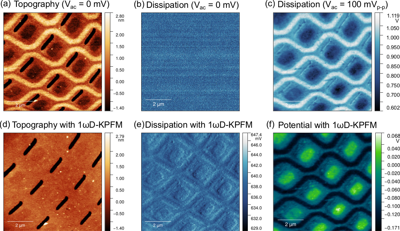
Figure 9: (a) Topography and (b) dissipation images of a CCD image sensor with FM mode with no ac voltage and a constant $V_{\mathrm{bias}}=50$ mV applied. $\Delta f=-0.3$ Hz. No contrast is observed in (b). (c) dissipation image with coherent ac voltage with FM mode with its amplitude, $V_{\mathrm{ac}}=100$ mV_p-p ($\omega_{\mathrm{el}}=\omega_{\mathrm{m}}$). The similar contrast to that appears in the topography (a) is observed. (e) topography, (f) dissipation, (g) potential images with $1\omega$D-KPFM technique with $V_{\mathrm{ac}}=100$ mV_p-p, $\omega_{\mathrm{el}}=\omega_{\mathrm{m}}$.

0.4.3 Comparison of different KPFM techniques

In this section, we compare the KPFM images taken with FM-KPFM, AM-KPFM, $1\omega$D-KPFM and $2\omega$D-KPFM to evaluate the performance of each technique. We used a patterned MoS₂ flake for the comparison. The several ten $\mu$m scale size of the sample together with the etched stripe pattern with 2 $\mu$m pitch enables to find the same region of the sample even in the separate runs. Flakes of MoS₂ were deposited onto a SiO₂/Si substrate by mechanical exfoliation and a stripe pattern was created by electron beam lithography and the subsequent reactive ion etching on top of the flakes. Fig. 10 shows the optical micrograph of the MoS₂ flake used for the KPFM imaging experiments.

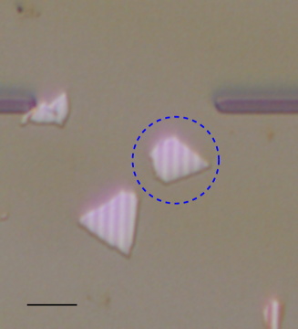
Figure 10: Optical micrograph of the patterned MoS₂ flakes exfoliated on SiO₂/Si substrate.The flake in the circle is the one imaged by the KPFM imaging experiments. Scale bar is 20 $\mu$m.

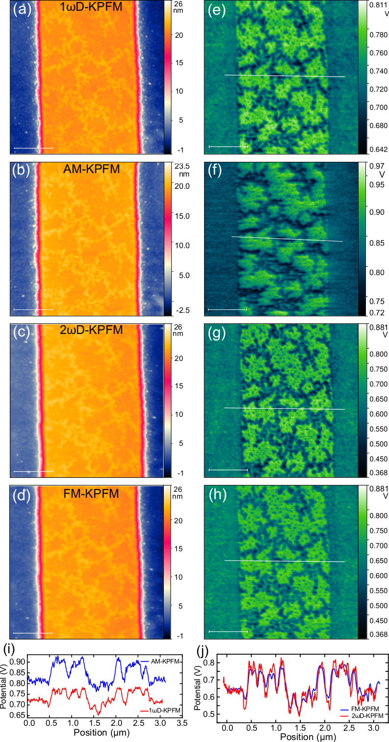
Figure 11: Topography and CPD images of the patterned MoS₂ flake. Topography images taken by (a) $1\omega$D-KPFM, (b) AM-KPFM, (c) $2\omega$D-KPFM and (d) FM-KPFM techniques. CPD images taken by (e) $1\omega$D-KPFM, (f) AM-KPFM, (g) $2\omega$D-KPFM and (h) FM-KPFM techniques. (i) Profiles of the CPD images by (e) $1\omega$D-KPFM and (f) AM-KPFM techniques. (j) Profiles of the CPD images by (g) $2\omega$D-KPFM and (h) FM-KPFM techniques

Fig. 11 shows topography and potential images of the patterned MoS₂ flake by (a) $1\omega$D-KPFM, (b) AM-KPFM, (c) $2\omega$D-KPFM and (d) FM-KPFM techniques. The $1\omega$D-KPFM, $2\omega$D-KPFM and FM-KPFM images were taken with the same cantilever tip ($f_{0}=306553$ Hz, $k=20.8$ N/m, $Q=14963$) and the AM-KPFM image was taken with a different one ($f_{0}=298044$ Hz, $k=27.2$ N/m, $Q=14700$). These two cantilevers were of the same type (NSC15, MikroMasch) and taken from the same batch. In $1\omega$D-KPFM imaging, a sinusoidally oscillating voltage with an amplitude of $V_{\mathrm{ac}}=100$ mV_p-p phase-locked with the tip oscillation was applied to the sample. In AM-KPFM imaging, a sinusoidally oscillating voltage with an amplitude of $V_{\mathrm{ac}}=8$ V_p-p whose frequency was tuned to the second flexural resonance peak (resonance frequency:1,903,500 Hz, quality factor:2400) was applied to the sample. The resulting oscillation amplitude was detected by a high-speed lock-in amplifier (HF2LI, Zurich Instruments) and used for the dc bias voltage feedback Kikukawa96 ; Sommerhalter1999 . In FM-KPFM imaging, a sinusoidally oscillating voltage with the amplitude of $V_{\mathrm{ac}}=2.0$ V_p-p and frequency of 300 Hz was applied to the sample Kitamura98 . The number of pixels in the images is 512$\times$512. The scanning time for $1\omega$D-KPFM, $2\omega$D-KPFM and FM-KPFM imaging was 512 s/frame (1 s/line). The scanning time for AM-KPFM was for 1024 s/frame (2 s/line). In all the imaging modes, the frequency shift signal was used for topography feedback.

The topography images (Fig. 11(a-d)) show an unetched terrace located between the etched regions. The height of the terrace is approximately 20 nm with respect to the etched regions. A clear fractal-like pattern can be seen on the terrace in all the CPD images. The potential contrast can be ascribed to the residue of the etch resist (PMMA) as the topography images show a similar contrast with a thickness of about 1 nm.

Comparison between $1\omega$D-KPFM and AM-KPFM

First, we compare the CPD images taken by $1\omega$D-KPFM (Fig. 11(a)) and AM-KPFM (Fig. 11(b)). The CPD image by $1\omega$D-KPFM shows better clarity than that by AM-KPFM. The difference is due to the lower signal-to-noise ratio of the amplitude signal of the second flexural mode oscillation despite that a much higher $V_{\mathrm{ac}}=8$ V_p-p was applied in AM-KPFM. The higher effective spring constant of the second flexural mode oscillation ($k_{\mathrm{2nd}}\sim 40\times k\approx 800$ N/m) compared to the first mode Kikukawa96 ; Melcher07 and lower observed quality factor ($Q_{\mathrm{2nd}}=2400$ compared with 14700 for the first mode) account for the difference as the signal in both operating modes is proportional to $Q/k$. Notice that the cantilevers with lower effective spring constant ($k\approx 2\sim 3$ N/m) have been used in the most reported AM-KPFM measurements in which $V_{\mathrm{ac}}$ of the order of 100 mV is employed Kikukawa96 ; Sommerhalter1999 ; Glatzel2003a ; Zerweck05 ; Burke09a . Fig. 11(i) shows the line profiles of potential on the same location indicated as a white line in the CPD images Fig. 11(e) and (f). Two profiles are in a very good agreement except the constant offset. This observed similarity can be understood by the fact that both $1\omega$D-KPFM and AM-KPFM are sensitive to the electrostatic force. The constant offset between two profiles is probably due to the different tips used in the two separate experiments.

Comparison between $2\omega$D-KPFM and FM-KPFM

Now we turn to the comparison between $2\omega$D-KPFM (Fig. 11(g)) and FM-KPFM (Fig. 11(h)). The CPD images taken with $2\omega$D-KPFM and FM-KPFM look very similar and the line profiles of two images taken on the same location indicated as a white line show a good agreement. A closer inspection reveals slightly larger potential contrast in the $2\omega$D-KPFM image compared with the FM-KPFM image, which is due to the faster KPFM feedback response of $2\omega$D-KPFM by virtue of the absence of low frequency modulation which is required for FM-AFM.

Comparison between $1\omega$D-KPFM and $2\omega$D-KPFM

Although both potential images taken with $1\omega$D-KPFM (Fig. 11(e)) and $2\omega$D-KPFM (Fig. 11(g)) show the almost identical pattern on the terrace with the nearly same signal-to-noise ratio, we notice lower contrast in the CPD image taken with $1\omega$D-KPFM than that with $2\omega$D-KPFM from the inspection of the line profiles, Fig. 11(i) and (j). The peak-to-peak value of the potential variation in the $1\omega$D-KPFM image is $\sim 0.12$ V, about one half that in the $2\omega$D-KPFM image ($\sim 0.3$ V). The similar difference in the potential contrast taken with FM-KPFM and AM-KPFM has also been reported in the literature and is ascribed to the fact that the AM-KPFM is sensitive to electrostatic force whereas FM-KPFM uses the modulation in the resonance frequency shift which is sensitive to force gradient Zerweck05 ; Glatzel2003a . As we have already discussed, the same argument applies to $1\omega$D-KPFM and $2\omega$D-KPFM. The smaller potential contrast observed in $1\omega$D-KPFM than in $2\omega$D-KPFM can be explained by larger spatial average due to the stray capacitance including the body of the tip and the cantilever  Hochwitz1996 ; Jacobs1999 ; Strassburg2005a ; Cohen2013 . We noticed that an ac voltage amplitude (2 V) much larger than that require for $1\omega$D-KPFM (100 mV) was necessary for $2\omega$D-KPFM. This indicates $\alpha>\alpha^{\prime}A$ which is determined by the distance dependence of the tip-sample capacitance. This condition could be changed by engineering the tip shape.

In spite of lower potential contrast, $1\omega$D-KPFM has a clear advantage in that it requires much smaller $V_{\mathrm{ac}}=100\,$mV_p-p compared with 2 V_p-p for $2\omega$D-KPFM. This advantage is important for electrical characterizations of technically relevant materials whose electrical properties are influenced by the externally applied electric field as is the case in semiconductors where the influence of the large $V_{\mathrm{ac}}$ can induce band-bending effects.

0.4.4 Dynamic response of D-KPFM

The detection bandwidth of D-KPFM is determined by the bandwidth of the amplitude control feedback loop used in FM-KPFM. In fact, we notice that applying the coherent $V_{\mathrm{ac}}$ causing dissipative force can be used to measure the dynamics of the amplitude control feedback system.

In FM-KPFM, the AFM cantilever serves as the frequency determining element of a self-driven oscillator so that the oscillation frequency keeps track of the resonance frequency of the cantilever. In this way, the conservative force has no influence on the drive amplitude (dissipation signal) when the time delay set by the phase shifter is property adjusted as already discussed in Sect. 0.2.1 whereas the amplitude controller compensates for the effective $Q$ factor change caused by dissipative force. Therefore, by modulating $V_{\mathrm{bias}}$ at a low frequency ($<$ a few kHz) together with applying the coherent $V_{\mathrm{ac}}$, the amplitude of the dissipative force can be modulated as can been seen in Eqs. 21 and  29 and the frequency response of the amplitude feedback loop can thus be measured by demodulating the dissipation signal with a lock-in amplifier. The measured $-3$ dB bandwidth of the amplitude feedback loop is as high as 1 kHz, which is wider than that of the typical PLL frequency detector (400 Hz in this experiment).

Notice that in contrast to the settling time of the oscillation amplitude of a cantilever subject to a change in conservative force which is $\tau\sim Q/f_{0}$ Albrecht1991 , the response time of the dissipation signal is not limited by $Q$ and can be faster because of the active damping mechanism built in the amplitude control feedback loop Durig1997 as well as the induced energy dissipation which is given by $\pi F_{\mathrm{quad}}A$ in addition to the internal dissipaiton of the cantilever, $\pi kA^{2}/Q$. The active damping behavior of the amplitude controller indeed manifests itself in the effective negative dissipation shown in $g$-$V_{\mathrm{bias}}$ curves (Figs. 5 and 7). This explains the observed fast response of the amplitude feedback loop, resulting in the wider bandwidth of the voltage feedback loop in D-KPFM than that in FM-KPFM that is limited by PLL demodulation bandwidth (typically $<1$ kHz) which sets the bias modulation frequency.

The low frequency $V_{\mathrm{bias}}$ modulation can also be used for D-KPFM imaging in the case where other dissipative interactions such as the Joule dissipation Denk91 and single-electron tunneling Cockins2010a ; Miyahara2017 or the dissipation artifact caused by the crosstalk to the frequency shift Labuda2011 contribute to the dissipation signal. It is possible to separate the induced electrostatic dissipation just as is done in FM-FKPFM with $\Delta f$ and in DM-KPFM with the tip oscillation amplitude Fukuma2004 . The modulated dissipation signal due to $V_{\mathrm{bias}}$ modulation can be demodulated with a lock-in amplifier which can then be used for the KPFM bias feedback.

0.5 Conclusion

We reported D-KPFM, a new experimental technique for KPFM in which the dissipation signal of FM-AFM is used for KPFM bias-voltage feedback. We show that D-KPFM can be operated in two different modes, $1\omega$D-KPFM and $2\omega$D-KPFM which are sensitive to electrostatic force and electrostatic force gradient, respectively. The technique features the simpler implementation and faster scanning than the most commonly used FM-KPFM technique as it requires no low frequency modulation.

We provided the theory of D-KPFM by combining two key aspects: (1) the effect of the periodically oscillating force on the resonant frequency shift and dissipation signal in FM-AFM and (2) the detail analysis of the electrostatic force by explicitly taking into account the effect of the tip oscillation.

We validated the theory by fitting with the experimental $\Delta f$-$V_{\mathrm{bias}}$ and $g$-$V_{\mathrm{bias}}$ curves in both $1\omega$ and $2\omega$D-KPFM cases. We experimentally showed the equivalence of $1\omega$D-KPFM and AM-KPFM and that of $2\omega$D-KPFM and FM-KPFM in terms of their sensitivity to electrostatic force and electrostatic force gradient, respectively. We demonstrated that $1\omega$D-KPFM requires a significantly smaller ac voltage amplitude (a few tens of mV) than $2\omega$D-KPFM and FM-KPFM. Even though the potential contrast obtained by $1\omega$D-KPFM is about two times smaller than that by $2\omega$D-KPFM, the use of the small ac voltage is of great advantage for characterizing materials whose properties are sensitive to the externally applied electric field such as semiconductors. The operations in $1\omega$ and $2\omega$D-KPFM can be switched easily to take advantage of both features at the same location on a sample.

References

- (1) M. Nonnenmacher, M.P. O’Boyle, H.K. Wickramasinghe, Appl. Phys. Lett. 58(25), 2921 (1991). DOI 10.1063/1.105227. URL http://aip.scitation.org/doi/10.1063/1.105227
- (2) A. Kikukawa, S. Hosaka, R. Imura, Rev. Sci. Instrum. 67(4), 1463 (1996). DOI 10.1063/1.1146874. URL http://aip.scitation.org/doi/10.1063/1.1146874
- (3) C. Sommerhalter, T.W. Matthes, T. Glatzel, A. Jäger-Waldau, M.C. Lux-Steiner, Appl. Phys. Lett. 75(2), 286 (1999). URL http://aip.scitation.org/doi/abs/10.1063/1.124357
- (4) U. Zerweck, C. Loppacher, T. Otto, S. Grafstrom, L.M. Eng, Phys. Rev. B 71(12), 125424 (2005). URL https://link.aps.org/doi/10.1103/PhysRevB.71.125424
- (5) S. Kitamura, M. Iwatsuki, Appl. Phys. Lett. 72(24), 3154 (1998). DOI 10.1063/1.121577. URL http://aip.scitation.org/doi/10.1063/1.121577
- (6) Z. Schumacher, Y. Miyahara, L. Aeschimann, P. Grütter, Beilstein Journal of Nanotechnology 6, 1450 (2015). DOI 10.3762/bjnano.6.150. URL http://www.beilstein-journals.org/bjnano/content/6/1/150
- (7) S.A. Burke, J.M. LeDue, Y. Miyahara, J.M. Topple, S. Fostner, P. Grutter, Nanotechnology 20(26), 264012 (2009). DOI 10.1088/0957-4484/20/26/264012. URL http://iopscience.iop.org/0957-4484/20/26/264012
- (8) Y. Miyahara, J. Topple, Z. Schumacher, P. Grutter, Phys. Rev. Applied 4(5), 054011 (2015). DOI 10.1103/PhysRevApplied.4.054011. URL http://link.aps.org/doi/10.1103/PhysRevApplied.4.054011
- (9) Y. Miyahara, P. Grutter, Applied Physics Letters 110(16), 163103 (2017). DOI 10.1063/1.4981937. URL http://aip.scitation.org/doi/10.1063/1.4981937
- (10) T. Fukuma, K. Kobayashi, H. Yamada, K. Matsushige, Rev. Sci. Instrum. 75(11), 4589 (2004). URL http://aip.scitation.org/doi/10.1063/1.1805291
- (11) H. Nomura, K. Kawasaki, T. Chikamoto, Y.J. Li, Y. Naitoh, M. Kageshima, Y. Sugawara, Appl. Phys. Lett. 90(3), 033118 (2007). DOI 10.1063/1.2432281. URL http://aip.scitation.org/doi/10.1063/1.2432281
- (12) T.R. Albrecht, P. Grutter, D. Horne, D. Rugar, Journal of Applied Physics 69(2), 668 (1991). DOI 10.1063/1.347347. URL http://aip.scitation.org/doi/10.1063/1.347347
- (13) U. Dürig, H.R. Steinauer, N. Blanc, Journal of Applied Physics 82(1997), 3641 (1997). DOI 10.1063/1.365726. URL http://aip.scitation.org/doi/10.1063/1.365726
- (14) A. Labuda, K. Kobayashi, Y. Miyahara, P. Grütter, Rev. Sci. Instrum. 83(May), 053703 (2012). DOI 10.1063/1.4712286. URL http://dx.doi.org/10.1063/1.4712286
- (15) A. Labuda, Y. Miyahara, L. Cockins, P. Grütter, Physical Review B 84(12), 125433 (2011). DOI 10.1103/PhysRevB.84.125433. URL http://link.aps.org/doi/10.1103/PhysRevB.84.125433
- (16) H. Hölscher, B. Gotsmann, W. Allers, U. Schwarz, H. Fuchs, R. Wiesendanger, Phys. Rev. B 64(7), 075402 (2001). DOI 10.1103/PhysRevB.64.075402. URL http://link.aps.org/doi/10.1103/PhysRevB.64.075402
- (17) L.N. Kantorovich, T. Trevethan, Phys. Rev. Lett. 93(23), 236102 (2004). DOI 10.1103/PhysRevLett.93.236102. URL http://link.aps.org/doi/10.1103/PhysRevLett.93.236102
- (18) J.E. Sader, T. Uchihashi, M.J. Higgins, A. Farrell, Y. Nakayama, S.P. Jarvis, Nanotechnology 16(3), S94 (2005). URL http://iopscience.iop.org/article/10.1088/0957-4484/16/3/018
- (19) Y. Miyahara, A. Roy-Gobeil, P. Grutter, Nanotechnology 28(6), 064001 (2017). DOI 10.1088/1361-6528/aa5261. URL http://doi.org/10.1088/1361-6528/aa5261
- (20) T. Fukuma, M. Kimura, K. Kobayashi, K. Matsushige, H. Yamada, Review of Scientific Instruments 76(5), 53704 (2005). URL http://aip.scitation.org/doi/10.1063/1.1896938
- (21) P. Zahl, T. Wagner, R. Möller, A. Klust, J. Vac. Sci. Technol. B Nanotechnol. Microelectron. 28(3), C4E39 (2010). DOI 10.1116/1.3374719. URL http://avs.scitation.org/doi/10.1116/1.3374719
- (22) H. Diesinger, D. Deresmes, J.P. Nys, T. Mélin, Ultramicroscopy 108(8), 773 (2008). DOI 10.1016/j.ultramic.2008.01.003. URL http://linkinghub.elsevier.com/retrieve/pii/S0304399108000132
- (23) T. Mélin, S. Barbet, H. Diesinger, D. Théron, D. Deresmes, Rev. Sci. Instrum. 82(3), 036101 (2011). DOI 10.1063/1.3516046. URL http://aip.scitation.org/doi/10.1063/1.3516046
- (24) S. Sadewasser, M. Lux-Steiner, Phys. Rev. Lett. 91(26), 1 (2003). DOI 10.1103/PhysRevLett.91.266101. URL http://link.aps.org/doi/10.1103/PhysRevLett.91.266101
- (25) Y. Miyahara, L. Cockins, P. Grutter, in Kelvin Probe Force Microscopy, ed. by S. Sadewasser, T. Glatzel (Springer Berlin Heidelberg, 2012), chap. 9, pp. 175–199. DOI 10.1007/978-3-642-22566-6-9. URL http://www.springer.com/materials/surfaces+interfaces/book/978-3-642-22565-9?changeHeader
- (26) W. Denk, D.W. Pohl, Applied Physics Letters 59(17), 2171 (1991). DOI 10.1063/1.106088. URL http://scitation.aip.org/content/aip/journal/apl/59/17/10.1063/1.106088
- (27) J. Melcher, S. Hu, A. Raman, Appl. Phys. Lett. 91(5), 53101 (2007). URL http://aip.scitation.org/doi/10.1063/1.2767173
- (28) T. Glatzel, S. Sadewasser, M. Lux-Steiner, Appl. Surf. Sci. 210(1-2), 84 (2003). DOI 10.1016/S0169-4332(02)01484-8. URL http://linkinghub.elsevier.com/retrieve/pii/S0169433202014848
- (29) T. Hochwitz, A.K. Henning, C. Levey, C. Daghlian, J. Vac. Sci. Technol. B Nanotechnol. Microelectron. 14(1), 457 (1996). DOI 10.1116/1.588494. URL http://scitation.aip.org/content/avs/journal/jvstb/14/1/10.1116/1.588494
- (30) H.O. Jacobs, H.F. Knapp, A. Stemmer, Review of Scientific Instruments 70(3), 1756 (1999). DOI 10.1063/1.1149664. URL http://aip.scitation.org/doi/10.1063/1.1149664
- (31) E. Strassburg, A. Boag, Y. Rosenwaks, Review of Scientific Instruments 76(8), 083705 (2005). DOI 10.1063/1.1988089. URL http://scitation.aip.org/content/aip/journal/rsi/76/8/10.1063/1.1988089
- (32) G. Cohen, E. Halpern, S.U. Nanayakkara, J.M. Luther, C. Held, R. Bennewitz, A. Boag, Y. Rosenwaks, Nanotechnology 24(29), 295702 (2013). DOI 10.1088/0957-4484/24/29/295702. URL http://iopscience.iop.org/article/10.1088/0957-4484/24/29/295702
- (33) L. Cockins, Y. Miyahara, S.D. Bennett, A.a. Clerk, S. Studenikin, P. Poole, A. Sachrajda, P. Grutter, Proc. Natl. Acad. Sci. U. S. A. 107(21), 9496 (2010). DOI 10.1073/pnas.0912716107. URL http://www.pnas.org/content/107/21/9496