Casimir Meets Poisson: Improved Quark/Gluon Discrimination with Counting Observables

Abstract

Charged track multiplicity is among the most powerful observables for discriminating quark- from gluon-initiated jets. Despite its utility, it is not infrared and collinear (IRC) safe, so perturbative calculations are limited to studying the energy evolution of multiplicity moments. While IRC-safe observables, like jet mass, are perturbatively calculable, their distributions often exhibit Casimir scaling, such that their quark/gluon discrimination power is limited by the ratio of quark to gluon color factors. In this paper, we introduce new IRC-safe counting observables whose discrimination performance exceeds that of jet mass and approaches that of track multiplicity. The key observation is that track multiplicity is approximately Poisson distributed, with more suppressed tails than the Sudakov peak structure from jet mass. By using an iterated version of the soft drop jet grooming algorithm, we can define a “soft drop multiplicity” which is Poisson distributed at leading-logarithmic accuracy. In addition, we calculate the next-to-leading-logarithmic corrections to this Poisson structure. If we allow the soft drop groomer to proceed to the end of the jet branching history, we can define a collinear-unsafe (but still infrared-safe) counting observable. Exploiting the universality of the collinear limit, we define generalized fragmentation functions to study the perturbative energy evolution of collinear-unsafe multiplicity.

1 Introduction

The fantastic jet reconstruction performance of ATLAS and CMS Aaboud:2017jcu ; Khachatryan:2016kdb —along with increasingly sophisticated tools to predict jet properties from first principles Dasgupta:2013ihk ; Frye:2016aiz ; Larkoski:2013paa ; Dasgupta:2015lxh ; Dasgupta:2014yra ; Larkoski:2015kga ; Procura:2014cba ; Waalewijn:2012sv —has led to significant advances in the field of jet substructure Adams:2015hiv ; Altheimer:2013yza ; Altheimer:2012mn ; Abdesselam:2010pt . A key goal in jet substructure is to robustly discriminate quark-initiated jets from gluon-initiated jets Gallicchio:2011xq ; Gallicchio:2012ez ; Larkoski:2013eya ; Larkoski:2014pca ; Bhattacherjee:2015psa ; Badger:2016bpw ; Komiske:2016rsd ; Davighi:2017hok ; Gras:2017jty , with many applications to new physics searches at the Large Hadron Collider (LHC) (see e.g. CMS:2013kfa ; FerreiradeLima:2016gcz ; Bhattacherjee:2016bpy ). In the eikonal limit, quarks and gluons differ only by their respective color charges, $C_{F}=4/3$ versus $C_{A}=3$, such that gluon jets emit more soft gluon radiation than quark jets. At this order, the difference between quark and gluon radiation patterns is controlled entirely by the Casimir ratio $C_{A}/C_{F}=9/4$, which drives (and limits) the expected separation power between quark and gluon jets.

One of the most powerful quark/gluon discriminants is hadron multiplicity, or its charged-particle-only variant, track multiplicity $n_{\rm tr}$ Gallicchio:2011xq ; Gallicchio:2012ez ; Aad:2014gea ; Larkoski:2014pca ; ATLAS:2016wzt ; Aad:2016oit . This is an effective discriminant because the average track multiplicity within quark and gluon jets scales approximately as (see e.g. Bolzoni:2012ii ; Bolzoni:2013rsa )

$$\frac{\langle n_{\rm tr}\rangle_{g}}{\langle n_{\rm tr}\rangle_{q}}\simeq\frac{C_{A}}{C_{F}}.$$ (1)

Since multiplicity is not infrared and collinear (IRC) safe, though, it is difficult to predict its discrimination performance from first principles. On the other hand, IRC-safe observables like jet mass and jet width are analytically tractable Banfi:2004yd ; Ellis:2010rwa ; Larkoski:2014uqa , but they exhibit worse quark/gluon performance than multiplicity. The reason is that these discriminants are dominated by a single emission at leading-logarithmic (LL) accuracy, giving rise to Casimir scaling of the quark/gluon discrimination power,

$$\text{(gluon mistag rate)}\simeq(\text{quark efficiency})^{C_{A}/C_{F}},$$ (2)

and therefore relatively weak separation between quark and gluon jets. This Casimir scaling behavior holds for any observable with a Sudakov form factor at LL accuracy, including a wide range of IRC-safe additive observables Larkoski:2013eya . While one can try to interpolate between the IRC-unsafe and IRC-safe regimes using generalized angularities Larkoski:2014pca , track multiplicity remains one of the best performing—yet analytically puzzling—quark/gluon discriminants.

In this paper, we introduce a new class of “counting observables” that are IRC safe, yet yield comparable quark/gluon performance to track multiplicity. Unlike additive observables, which are only sensitive to a single emission at LL order, these counting observables are directly sensitive to multiple emissions at LL, allowing them to exceed the performance estimate in Eq. (2). Crucially, the quark/gluon performance of counting observables still depends on the color factors $C_{A}$ and $C_{F}$, but instead of being described by Sudakov form factors, these observables are described by Poisson distributions; this allows their discrimination power to improve as more emissions are included. These counting observables not only clarify the underlying reason why track multiplicity performs so well, but they also demonstrate the new kinds of analytic structures possible from IRC-safe but non-additive observables.

The counting observables we study are based on an iterated variant of soft drop declustering Larkoski:2014wba . As a grooming procedure, soft drop starts at the trunk of an angular-ordered clustering tree Dokshitzer:1997in ; Wobisch:1998wt and sequentially removes soft branches with small momentum fraction $z_{ij}$ until a hard branching is found. At a step in the clustering tree where branches $i$ and $j$ split, the splitting is retained in the groomed jet if the momentum fraction satisfies

$$z_{ij}>{z_{\text{cut}}}\left(\frac{\theta_{ij}}{R_{0}}\right)^{\beta}\,,$$ (3)

where $\theta_{ij}$ is an appropriately defined relative angle between branches $i$ and $j$, and $R_{0}$ is the jet radius. For appropriate choices of the soft drop parameters ${z_{\text{cut}}}$ and $\beta$, observables defined on the groomed jet are automatically infrared (but not necessarily collinear) safe. While the original soft drop procedure terminates once it finds a hard $1\to 2$ splitting, the iterated variant we employ in this paper continues, following the hardest branch (the “trunk”) through multiple levels until an angular cutoff scale ${\theta_{\text{cut}}}$ is reached.

The simplest counting observable we can define using iterated soft drop (ISD) is just the total number of emissions from the trunk of the clustering tree that ISD records. In particular, this includes all emissions $n\in[1,n_{\rm max}]$ that satisfy the soft drop condition and lie outside the ${\theta_{\text{cut}}}$ cone. We call this observable “soft drop multiplicity”,

$$n_{\text{SD}}(z_{\rm cut},\beta,{\theta_{\text{cut}}})=\sum_{n}1,$$ (4)

which depends on the choice of ISD parameters. It is complementary to the “soft drop level” observable $L_{\text{SD}}(\beta)$ introduced in Ref. Aad:2015rpa , which also iteratively applies the soft drop condition, but changes the $z_{\rm cut}$ scale. As long as ${z_{\text{cut}}}>0$, soft drop multiplicity is infrared safe.

With ${\theta_{\text{cut}}}>0$ or $\beta<0$, $n_{\text{SD}}$ is collinear safe as well, so we can use analytic resummation tools to predict its discrimination power. We do this to resum large logarithms of ${z_{\text{cut}}}$ and ${\theta_{\text{cut}}}$, which are of soft and collinear origin, respectively, and which lead to a double-logarithmic observable. The analysis at LL order is straightforward, yielding a Poisson distribution whose average value is set by the phase space “area” of counted emissions. This leads to quark/gluon discrimination power which approaches that of track multiplicity, particularly in the case of $\beta=-1$. Moving from LL to next-to-leading-logarithmic (NLL) order, one finds a slight decrease in discrimination power, due in part to the jet-flavor mixing that appears at this accuracy. We implement the NLL calculation through a set of evolution equations that have a similar form to parton evolution.

With ${\theta_{\text{cut}}}=0$ and $\beta\geq 0$, the soft drop multiplicity $n_{\text{SD}}$ is no longer collinear safe, so we cannot predict its absolute discrimination power. That said, for the special case of $\beta=0$ (which was initially introduced as the modified mass drop tagger Dasgupta:2013ihk ; Dasgupta:2013via ), we can use renormalization group (RG) techniques to predict the evolution of its discrimination power. When $\beta=0$, soft drop multiplicity has purely collinear divergences, which can be absorbed into a generalized fragmentation function (GFF) that depends on the RG scale $\mu$ Elder:2017bkd . After extracting this GFF at low scales (either from LHC data or parton shower simulations), one can use a perturbative DGLAP-like evolution equation to predict the discrimination power achievable at higher scales. Intriguingly, in the limit of pure Yang-Mills, one can show that at lowest order, the soft drop multiplicity asymptotes to a true Poisson distribution at large values of $\mu$, such that it behaves like an idealized counting observable (albeit in a theory with only gluons).

The remainder of this paper is organized as follows. In Sec. 2, we define the ISD procedure, introduce soft drop multiplicity, and take a first look at its distribution using parton shower generators. In Sec. 3, we perform an LL analysis, focusing on the contrast between soft drop multiplicity’s Poisson behavior and the more familiar Sudakov-peak behavior of additive observables. We extend our analytic calculations to NLL order in Sec. 4 and compare our analytic distributions to those obtained from various parton showers. We consider the collinear-unsafe case of ${\theta_{\text{cut}}}=0$ and $\beta=0$ in Sec. 5, deriving the corresponding RG evolution equations and presenting numerical results based on parton shower inputs. We present our conclusions in Sec. 6.

In an appendix, we demonstrate that our analytical tools can also be used to study more general ISD observables, in particular the weighted multiplicity $\sum_{n}(z_{n})^{\kappa}$ which weights each counted emission according to its momentum fraction $z_{n}$. Soft drop multiplicity is a special case $(\kappa=0)$ of this more general observable, and the one most useful for quark/gluon discrimination.

2 Counting Observables from Soft Drop Declustering

2.1 Iterated Soft Drop

Our counting observables are defined using an iterated variant of the soft drop declustering algorithm. We briefly review soft drop here for convenience and to establish conventions.

The soft drop grooming procedure can be applied to any jet found using a standard jet algorithm of characteristic radius $R_{0}$. After reclustering the jet using the Cambridge/Aachen (C/A) algorithm Dokshitzer:1997in ; Wobisch:1998wt , soft drop involves sequentially undoing the cluster history to remove wide-angle soft radiation and identify hard 2-prong substructure. For each C/A branching into subjets $i$ and $j$, there are quantities $z_{ij}$ and $\theta_{ij}$, which are defined differently for different collider environments:

$$e^{+}e^{-} z_{ij} ={\min(E_{i},E_{j})\over E_{i}+E_{j}}\,, \theta_{ij} =\text{angle between $i,j$}\,,$$ collisions: (5)

$$pp z_{ij} ={\min(p_{Ti},p_{Tj})\over p_{Ti}+p_{Tj}}\,, \theta_{ij} =\Delta R_{ij}\,,$$ collisions: (6)

where $\Delta R$ represents distance in the rapidity-azimuth plane. The soft drop grooming algorithm can be summarized as follows:

1. Traverse the C/A clustering tree, beginning at the trunk and sequentially examining each branching.

2. Upon arriving at a branching into subjets $i$ and $j$, check whether the soft drop condition is satisfied:

   $$z_{ij}>{z_{\text{cut}}}\,\left({\theta_{ij}\over R_{0}}\right)^{\beta}\,,$$ (7)

   where ${z_{\text{cut}}}$ and $\beta$ are fixed parameters of the algorithm. If so, the algorithm terminates; stop grooming and return the jet as is.

3. If the branching fails this condition, remove the softer of the two subjets ($i$ or $j$) from the groomed jet and return to Step 2 on the next branching in the remaining clustering tree.

Our analysis is based on ISD where the soft drop algorithm is iterated. In this case, the procedure does not terminate when a hard branching is found, but is instead iteratively applied to the harder of the two subjets. This continues until an angular cutoff is reached, so in addition to ${z_{\text{cut}}}$ and $\beta$, ISD depends on an additional parameter ${\theta_{\text{cut}}}$. While ISD could be used as a grooming procedure in its own right, the primary purpose of ISD in this paper is to determine which set of $(z_{ij},\theta_{ij})$ branchings contribute to the observables we define below. For this purpose, the ISD algorithm proceeds as follows:

1. Set the counter $n$ equal to 1. Traverse the C/A clustering tree, beginning at the trunk and sequentially examining each branching.

2. Upon arriving at a branching into subjets $i$ and $j$, check whether the branching angle satisfies

   $$\theta_{ij}>{\theta_{\text{cut}}}\,.$$ (8)

   If not, the algorithm terminates.

3. If $\theta_{ij}>{\theta_{\text{cut}}}$, then check whether the soft drop condition is satisfied:

   $$z_{ij}>{z_{\text{cut}}}\,\left({\theta_{ij}\over R_{0}}\right)^{\beta}\,.$$ (9)

   If not, return to Step $2^{\prime}$ on the harder of subjets $i$ and $j$.

4. If the soft drop condition is satisfied, define

   $$z_{n}\equiv z_{ij}\,,\qquad\theta_{n}\equiv\theta_{ij}\,.$$ (10)

   Then increment $n\to n+1$ and return to Step $2^{\prime}$ on the harder of subjets $i$ and $j$.

Because we recurse to the harder subjet at each junction, we think of each $(z_{n},\theta_{n})$ splitting as an emission from the “hard core” of the jet and refer to the above procedure as traversing the “trunk” of the clustering tree. A schematic of this procedure is shown in Fig. 1.

Figure 1: Illustration of the ISD procedure. A C/A tree is declustered from the trunk (thick line), defined by the hardest $p_{T}$ branches. If a node fails the soft drop condition, it is removed from consideration (dashed lines). If a node passes the soft drop condition after $n$ iterations, this defines the value of $(z_{n},\theta_{n})$. The declustering stops at an angular scale of $\theta_{\rm cut}$, and subsequent nodes are not considered further (gray lines).

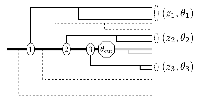
To emphasize, we are not using ISD as an alternative grooming technique to soft drop. In fact, we have found no need to refer to the ISD-groomed jet explicitly in our analysis. Instead, we employ ISD simply as a method to obtain an IRC-safe set of $(z_{n},\theta_{n})$ values to define our counting observables. Of course, the specific values of $(z_{n},\theta_{n})$ depend on the precise choice of ISD procedure. In this paper, we focus on the soft drop multiplicity, which counts emissions from the trunk of the clustering tree, and have defined ISD accordingly. In Sec. 2.3, we consider variants of soft drop multiplicity, with corresponding variants to the ISD procedure.

To demonstrate the qualitative behavior of observables defined below in this section, we present results from parton shower simulations. We separately generate $pp\to Z+q$ and $pp\to Z+g$ events at center-of-mass energy 13 TeV using MadGraph 2.4.0 and let the $Z$ decay to neutrinos for simplicity. We then shower the events through Vincia 2.0.01 Giele:2007di ; Giele:2011cb , a plug-in to Pythia 8.215 Sjostrand:2007gs , with default tuning parameters. Jet are identified using the anti-$k_{t}$ algorithm Cacciari:2008gp with radius $R_{0}=0.6$ in FastJet 3.1.3 Cacciari:2011ma . We use a sample of events in which the hardest jet with $|\eta|<2.5$ has $p_{T}$ between 450 and 550 GeV. We recluster and measure our observables on the hardest jet from each event using FastJet. Because ISD is sufficiently different from ordinary soft drop, we do not use the RecursiveTools fjcontrib fjcontrib , but rather directly traverse the C/A tree in our analysis. We plan to make our code available publicly in a future release of fjcontrib.

2.2 Soft Drop Multiplicity

The $(z_{n},\theta_{n})$ values from ISD allow us to define a variety of interesting jet observables. Here, we focus on soft drop multiplicity $n_{\text{SD}}$, which is simply the total count of the recorded $(z_{n},\theta_{n})$ pairs. This observable, defined already in Eq. (4), depends implicitly on the ISD parameters ${z_{\text{cut}}}$, $\beta$, and ${\theta_{\text{cut}}}$. Among all of the observables we tested, $n_{\text{SD}}$ appears to perform the best for quark/gluon discrimination. We discuss more general observables in Sec. 2.3 and App. A.

As defined above, ISD only follows the harder branch (i.e. the trunk) at each junction of the clustering tree. Therefore, $n_{\text{SD}}$ effectively counts emissions from the hard core of the jet, down to the angular resolution scale ${\theta_{\text{cut}}}$. When ${z_{\text{cut}}}={\theta_{\text{cut}}}=0$, $n_{\text{SD}}$ is simply the depth of the trunk of the C/A tree.

When ${z_{\text{cut}}}>0$, the soft drop multiplicity is infrared safe, as all soft emissions at finite angles fail the soft drop condition in Eq. (9). When ${\theta_{\text{cut}}}>0$, soft drop multiplicity is also collinear safe, since an exactly collinear splitting along the trunk does not satisfy Eq. (8). Alternatively, $\beta<0$ also gives collinear-safe distributions, since an exactly collinear splitting along the trunk does not satisfy Eq. (9). The borderline case of ${\theta_{\text{cut}}}=0$ and $\beta=0$ is collinear unsafe, but it can be handled using RG methods, as shown in Sec. 5.

Figure 2: Distribution of the soft drop multiplicity $n_{\text{SD}}$ from Vincia 2.0.01. Using the IRC-safe benchmark parameters in Eq. (11), we find good quark/gluon discrimination power. For comparison, we show Poisson distributions with the same means as dashed curves ($\lambda_{q}=2.2$, $\lambda_{g}=4.3$).

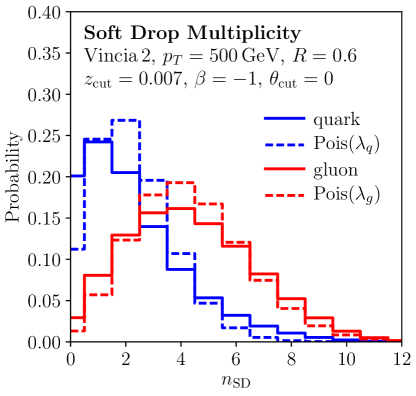
In Fig. 2, we show the soft drop multiplicity distributions for quark and gluon jets as extracted from Vincia. Results are given using the benchmark parameters

$${z_{\text{cut}}}=0.007\,,\qquad\beta=-1\,,\qquad{\theta_{\text{cut}}}=0\,.$$ (11)

This benchmark is chosen to maximize quark/gluon discrimination power while retaining perturbative calculability, as discussed in Sec. 3. The distributions are approximately Poisson and yield good quark/gluon discrimination power.

2.3 Multiplicity Variants

While the focus of this paper is on soft drop multiplicity $n_{\text{SD}}$, many other observables could be defined using the $(z_{n},\theta_{n})$ values recorded by ISD. For example, the techniques developed in this paper can be directly applied to the weighted soft drop multiplicity,

$$n_{\text{SD}}^{(\kappa)}=\sum_{n}z_{n}^{\kappa}\,.$$ (12)

Note that soft drop multiplicity is a special case ($\kappa=0$) of this more general observable, with the same criteria for IRC safety. We study the weighted multiplicity in detail in App. A, but find its quark/gluon discrimination power to be inferior to the discrete $\kappa=0$ case. In fact, LL reasoning leads one to expect the soft drop multiplicity $n_{\text{SD}}$ to have the best discrimination power of any observable defined on the $(z_{n},\theta_{n})$ values; see the end of Sec. 3.3 for a short discussion.

Nevertheless, several other promising variants of soft drop multiplicity might prove useful:

• The weighted soft drop multiplicity in Eq. (12) only refers to the momentum fractions $z_{n}$ in the sum over emissions. One could also consider an angle-weighted variant

  $$\sum_{n}z_{n}^{\kappa}\,\theta_{n}^{\alpha}\,,$$ (13)

  or indeed any function of $z_{n}$ and $\theta_{n}$. The potential advantage of including $\theta_{n}$ information is that even for ${\theta_{\text{cut}}}=0$, such observables would be collinear safe for $\alpha>0$.

• Instead of counting emissions only from the trunk of the C/A tree, we could extend the sum to include all branchings down to the angular resolution ${\theta_{\text{cut}}}$. This multiplicity variant would require a modification of the ISD algorithm: in step $4^{\prime}$, the recursion would be applied to both subjets $i$ and $j$, not just the harder one. This is a step in similarity towards full hadron multiplicity, reducing to it exactly when ${z_{\text{cut}}}={\theta_{\text{cut}}}=0$. This variant of soft drop multiplicity is more difficult to study analytically, however, due to the nonlinear structure of the recursion. Moreover, it is not clear that this variant would provide a performance advantage over $n_{\text{SD}}$. While gluons emitted from the hard core of a quark (gluon) jet give rise to factors of $C_{F}$ ($C_{A}$), subsequent emissions from those gluons give rise to factors of $C_{A}$ regardless of the jet flavor; this might wash out quark/gluon discrimination power.

• The original soft drop algorithm uses a C/A tree to mimic the angular-ordered structure of the parton shower. One could also study variants based on reclustering with the generalized-$k_{t}$ algorithm with exponent $p$ Cacciari:2008gp ; Cacciari:2011ma . The C/A algorithm used above corresponds to $p=0$, while the $k_{t}$ algorithm uses $p=1$. For this variant, it would make sense to replace the angular cut ${\theta_{\text{cut}}}$ with a cut $d_{\text{cut}}$ on the generalized distance measure $d_{ij}$.

This last $k_{t}$ variant is of particular interest, given the discussion below in Sec. 3.3. Nonperturbative physics typically dominates when $k_{t}\simeq\Lambda_{\rm QCD}$, so it makes sense to use a clustering algorithm where the clustering scale is “parallel” to the nonperturbative scale. This variant of $n_{\text{SD}}$ would then allow the nonperturbative phase space to be clearly separated from the perturbative region and avoided. This would open up as much perturbative phase space for measured emissions as possible. We note that it is possible to mimic some of the LL structure of the $k_{t}$ variant by using ISD with $\beta=-1$, though there would be differences going to NLL order.

We defer an analysis of these variants to future work, anticipating that many of the analytic tools from this paper can be translated to these generalized contexts. Experimentally, one might want to measure a track-based version of $n_{\text{SD}}$, trading collinear safety for improved robustness to pileup, which could be studied with the help of track functions Chang:2013rca ; Chang:2013iba ; Elder:2017bkd .

3 Leading-Logarithmic Analysis

At LL order, the only difference between quarks and gluons is encoded in the color factors $C_{F}$ and $C_{A}$, so Casimir scaling is a generic feature of many quark/gluon discriminants. Here, we review the case of additive observables (and close variants), where Casimir scaling of the Sudakov form factor yields a universal discrimination power at LL that depends only on $C_{A}/C_{F}$. We then show that the soft drop multiplicity is Poisson distributed, with its mean and variance satisfying Casimir scaling.

In general, any observable that is sensitive to multiple emissions at LL is “Poisson-like” distributed, in the sense that its variance $\sigma^{2}$ and mean $\mu$ both scale with the number $n$ of emissions counted, i.e. $\sigma^{2}=\mathcal{O}(\mu)$. In the limit of many emissions, all such observables converge to a normal distribution with decreasing relative width $w_{\rm rel}\sim\sigma/\mu\sim 1/\sqrt{n}$. Then as more emissions are counted, the discrimination power is not a universal function of $C_{A}/C_{F}$, but instead improves as $\mu$ increases and the quark/gluon distributions separate.

In this section, we illustrate this behavior for soft drop multiplicity with distributions extracted from Vincia, using the setup described in Sec. 2.1. We extract ROC (receiver operating characteristic) curves of the quark efficiency versus the gluon mistag rate, and explain their qualitative behavior. In App. A, we consider weighted soft drop multiplicity, with behavior that interpolates between that of Poisson- and Sudakov-distributed observables.

3.1 Review of Additive Observables

A generic jet observable is defined on the momenta $p_{i}$ and quantum numbers $q_{i}$ of particles within a jet. An additive IRC-safe observable $f$ is one that reduces to the form

$$f\left(\{p_{i},q_{i}\}\right)=\sum_{i\in\text{jet}}f(p_{i})$$ (14)

in the soft/collinear limit, so that the observable depends on a simple sum over the jet constituents, independent of $q_{i}$. The function $f(p_{i})$ can depend on global properties of the jet (e.g. its $p_{T}$), but not on its substructure. Collinear safety implies that $f(p_{i})$ is linear in the particle energies $E_{i}$. Examples of additive observables include the jet mass Clavelli:1979md ; Catani:1991bd ; Catani:1992ua , the radial moments Gallicchio:2010dq , and the angularities Berger:2003iw ; Almeida:2008yp ; Ellis:2010rwa , among many others.

(a)

(b)

Figure 3: Illustration of emission phase space, which is a close analog of the Lund diagram Andersson:1988gp , where gluon emissions are uniformly distributed in the $(\log 1/\theta,\log 1/z)$ plane. (a) The measurement of an additive observable $f$ imposes a Sudakov veto on the phase space area $A(f)$. (b) For groomed observables, the measurement of a quasi-additive observable $f_{\rm groomed}$ also imposes a Sudakov veto.

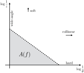
We now review the Casimir scaling of additive observables at LL order, as discussed in Ref. Larkoski:2013eya . For simplicity of the discussion below, we let $\alpha_{s}$ be a fixed coupling so that the expressions are more compact, but it is straightforward to include a running coupling at LL order. At this order, we need only consider gluon emissions from the jet core that are both soft and collinear, described by the most singular terms in the splitting function. Parametrizing emissions by their angle $\theta$ and energy (or $p_{T}$) fraction $z$, real emissions are uniformly distributed in the $(\log 1/\theta,\log 1/z)$ plane. The density in this emission phase space is

$$\rho_{i}=\frac{2\alpha_{s}C_{i}}{\pi},$$ (15)

where $C_{i}$ is the appropriate color factor, equal to $C_{F}=4/3$ for quarks and $C_{A}=3$ for gluons. The structure of emission phase space is shown in Fig. 3a. Virtual emissions are encoded in the boundaries of the emission phase space, where $\log(1/\theta),\log(1/z)\to\infty$, such that the total emission probability at each $\alpha_{s}$ order is zero to maintain the normalization of the probability distribution.

Applying the strongly-ordered limit and the fact that $f(p_{i})$ is linear in $E_{i}$, only a single dominant emission contributes to the observable at lowest order:

$$\sum_{i\in\text{jet}}f(p_{i})\quad\mathop{\Longrightarrow}^{\text{LL}}\quad\max_{i\in\text{jet}}f(p_{i}).$$ (16)

Therefore, the probability that the observable $f$ is less than some value $f_{\text{max}}$ is equal to the probability that there are no emissions in the region where $f(p_{i})>f_{\text{max}}$. This implies a cumulative distribution function

$$\int_{0}^{f_{\text{max}}}\text{d}f\,p(f)\equiv\Sigma_{i}(f_{\text{max}})=e^{-\rho_{i}A(f_{\text{max}})}\,,$$ (17)

where $A(f_{\text{max}})$ is the forbidden area of emission phase space, shown in Fig. 3a:

$$A(f_{\text{max}})=\int_{f(z,\theta)>f_{\text{max}}}\frac{\text{d}\theta}{\theta}\frac{\text{d}z}{z}.$$ (18)

Note that the cumulative distributions for quarks and gluons are related by

$$\Sigma_{g}(f_{\text{max}})=\Bigl{[}\Sigma_{q}(f_{\text{max}})\Bigr{]}^{C_{A}/C_{F}},$$ (19)

where $C_{A}/C_{F}=9/4$. That is, the Sudakov form factors for $f$ are related by Casimir scaling. As a result, the ROC curve for quark/gluon discrimination, which simply plots $\Sigma_{q}(f)$ versus $\Sigma_{g}(f)$, takes the universal form of Eq. (2).

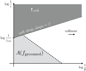
From this logic, it is clear that the above analysis also extends to certain non-additive observables. For example, jet observables defined on groomed jets are not additive, since the grooming procedure removes emissions that would otherwise contribute to the sum in Eq. (14). But groomed observables of the quasi-additive form

$$f_{\rm groomed}\left(\{p_{i},q_{i}\}\right)=\sum_{i\in\text{groomed jet}}f(p_{i})$$ (20)

still exhibit Casimir scaling, since the measured value of $f_{\rm groomed}$ forbid emissions in the region $A(f_{\rm groomed})$ shown in Fig. 3b. More generally, Casimir scaling arises whenever the value of the measurement actively forbids emissions from some region of phase space. This vetoed phase space region builds up a Sudakov form factor which in turn controls the discrimination power achievable at LL.

Figure 4: Comparison of the quark/gluon ROC curves for various Sudakov-distributed observables to the $y=x^{9/4}$ prediction from Casimir scaling. Shown are the groomed jet radius, groomed jet mass, and ordinary jet mass. As a useful benchmark, we also show the performance of track multiplicity $n_{\rm tr}$, which is known to be a very strong discriminant.

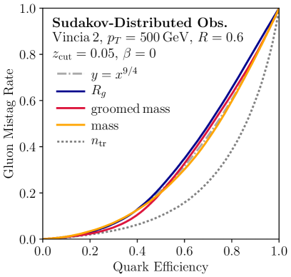
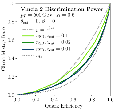
Beyond LL order, different Sudakov-distributed observables will exhibit different discrimination power due to higher-order or nonperturbative effects, but Eq. (19) is still a representative benchmark. In Fig. 4, we show ROC curves for jet mass $m$, the soft-dropped jet mass $m_{\text{SD}}$, and the groomed jet radius $R_{g}$, which all roughly follow the prediction from Casimir scaling. We also show track multiplicity $n_{\rm tr}$, which exhibits substantially better performance and provides a useful discrimination target.

3.2 Soft Drop Multiplicity

Figure 5: Same as Fig. 3b, but now highlighting the allowed emission region $A_{\text{emit}}$ that is counted by soft drop multiplicity.

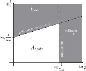
Soft drop multiplicity is not an additive observable, nor does the measured value of $n_{\text{SD}}$ actively forbid emissions in any region of phase space. As a result, $n_{\text{SD}}$ does not exhibit Sudakov behavior and it instead satisfies a fundamentally different scaling relation. Physically, this is because all emissions that pass the soft drop condition are weighted equally, so $n_{\text{SD}}$ depends on multiple emissions even at leading accuracy. These emissions occur in the region of phase space passing the soft drop and angular cuts, shown in Fig. 5.

Restricting to the IRC safe case with ${\theta_{\text{cut}}}>0$, the measured region has finite area in the emission plane,

$$A_{\text{emit}}=\log\frac{R_{0}}{{\theta_{\text{cut}}}}\left(\log\frac{1}{2{z_{\text{cut}}}}+\frac{\beta}{2}\log\frac{R_{0}}{{\theta_{\text{cut}}}}\right),$$ (21)

and soft drop multiplicity simply counts the number of real emissions in this area. This expression actually holds for all $\beta\in(-\infty,\infty)$ as long as the angular cut ${\theta_{\text{cut}}}$ imposes a non-trivial constraint on emissions. Since real emissions occur independently with uniform probability, they are described by a Poisson process, and the soft drop multiplicity is Poisson distributed at LL order:

$$\mathcal{P}_{i}(n_{\text{SD}})=\text{Pois}(\lambda_{i})[n_{\text{SD}}],\qquad\lambda_{i}=\rho_{i}A_{\text{emit}}.$$ (22)

For reference, the Poisson distribution with mean $\lambda$ is

$$\text{Pois}(\lambda)[n]=\frac{\lambda^{n}e^{-\lambda}}{n!}.$$ (23)

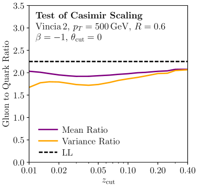
Since the variance of a Poisson distribution is also equal to $\lambda$, the means and variances of $n_{\text{SD}}$ both satisfy Casimir scaling

$$\frac{\langle n_{\text{SD}}\rangle_{g}}{\langle n_{\text{SD}}\rangle_{q}}\simeq\frac{C_{A}}{C_{F}},\qquad\frac{\text{Var}(n_{\text{SD}})_{g}}{\text{Var}(n_{\text{SD}})_{q}}\simeq\frac{C_{A}}{C_{F}},$$ (24)

mirroring the behavior of track multiplicity in Eq. (1), but for an IRC-safe observable.

To be clear, in defining our resummation accuracy, we count large logarithms of ${z_{\text{cut}}}$ and ${\theta_{\text{cut}}}$ in the mean/variance of the $n_{\text{SD}}$ distribution. That is, we define LL and NLL exactly as for more familiar additive observables, with LL including all terms of the form $\alpha_{s}^{n}\log^{n+1}$ that appear in the exponent of the $n_{\text{SD}}$ distribution, and NLL including those terms of the form $\alpha_{s}^{n}\log^{n}$. With this definition, Eq. (21) then shows that $n_{\text{SD}}$ is indeed a double-logarithmic observable. In this section, we study this observable’s general properties with fixed coupling, i.e. in the double-logarithmic approximation, for purposes of illustration. In Sec. 4, LL and NLL results are computed using the appropriate running coupling.

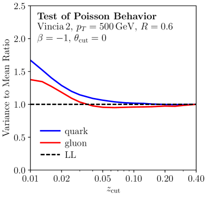
The above analysis provides several concrete predictions. Our most salient result is that, since the soft drop multiplicity is Poisson distributed at LL, we expect the ratio of the variance to the mean to be close to 1, as shown in Fig. 6a. We also predict that the mean and variance satisfy the Casimir scaling relations in Eq. (24), as shown in Fig. 6b. Though not shown here, we also checked the prediction that for $\beta=0$, the mean soft drop multiplicity scales as

$$\lambda_{i}\propto\log\frac{1}{z_{\mathrm{cut}}}\log\frac{1}{\theta_{\mathrm{cut}}}.$$ (25)

In general, we find good agreement for these predictions at large values of $z_{\mathrm{cut}}$, even out to $z_{\mathrm{cut}}\simeq 0.4$ where $\log z_{\mathrm{cut}}$ is not so large. For lower cut values, nonperturbative and higher-order effects cause these LL results to break down. In Sec. 3.3, we demonstrate how to choose parameters so that nonperturbative effects can be avoided, and in Sec. 4.2, we compute the NLL corrections to the perturbative predictions discussed here.

(a)

(b)

Figure 6: (a) Variance to mean ratio of the soft drop multiplicity as a function of $z_{\mathrm{cut}}$. The parameters $\beta$ and $\theta_{\mathrm{cut}}$ are set to the benchmark values in Eq. (11), and the LL prediction of equal mean and variance is shown as a dashed line. (b) Gluon to quark mean ratios and variance ratios, with the prediction of Casimir scaling shown as a dashed line. In both cases, we see qualitative agreement between Vincia and the LL predictions down to $z_{\mathrm{cut}}=0.02$.

Figure 7: Expected quark/gluon discrimination power for Poisson-distributed observables. The mean observable value for quarks is $\lambda_{q}$, and we assume the mean for gluons is given by Casimir scaling $\lambda_{g}=(C_{A}/C_{F})\lambda_{q}$. For reference, we show the $y=x^{9/4}$ curve for additive observables with Casimir scaling, as well as track multiplicity $n_{\rm tr}$ extracted from Vincia. For mean quark values $\lambda_{q}\gtrsim 2$, a Poisson-like observable satisfying Casimir scaling would be competitive with track multiplicity. The ROC curves are piecewise linear since the observable takes on discrete integer values.

3.3 Optimal Discrimination Power

As a direct result of the properties exhibited in Sec. 3.2, the discrimination power of soft drop multiplicity improves as the means $\lambda_{i}=\rho_{i}A_{\text{emit}}$ increase. This is because the mean of each distribution is proportional to the Casimir $C_{i}$, while the standard deviation is equal to the square root of the mean. The overlap of the distributions is characterized by the relative width

$$w_{\text{rel}}\equiv\frac{\sqrt{\text{Var}(n_{\text{SD}})_{i}}}{\langle n_{\text{SD}}\rangle_{i}}=\frac{1}{\sqrt{\lambda_{i}}}.$$ (26)

Indeed, in the many-emission limit where the distributions are approximately Gaussian, have equal mean and variance, and satisfy Casimir scaling, the discrimination power is solely determined by the relative width. As the cuts $z_{\mathrm{cut}}$ and $\theta_{\mathrm{cut}}$ are lowered, the means increase, causing the relative widths to narrow, reducing the overlap between the quark and gluon distributions, and improving the discrimination power.

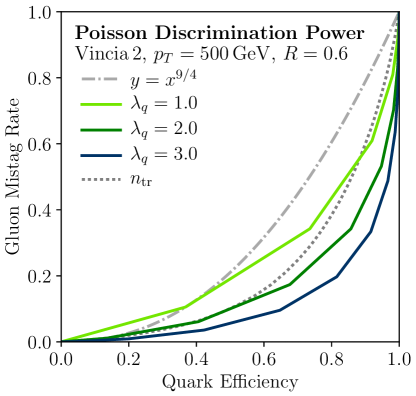
For reference, the discrimination power of Poisson distributions with different means is shown in Fig. 7, from which we see that track multiplicity has comparable discrimination power to a $\lambda_{q}\simeq 2$ observable.

To maximize the quark/gluon discrimination power, one should maximize the mean of the soft drop multiplicity distributions, which corresponds to taking ${z_{\text{cut}}}$ and ${\theta_{\text{cut}}}$ as small as possible, for a given exponent $\beta$. The validity of this analysis, however, is restricted to perturbation theory, so we must ensure that the values of the chosen parameters do not allow for distributions that are dominated by nonperturbative emissions. We can determine the parameters that enforce perturbative emissions by restricting the minimum relative $k_{t}$ appropriately.

(a)

(b)

Figure 8: Illustration of the optimal phase space configuration consistent with a perturbative analysis. The dashed line with slope $-1$ separates perturbative and nonperturbative emissions. (a) For $\beta>-1$, the value of $\theta_{\rm cut}$ has to be chosen to avoid allowed emissions above the nonperturbative boundary. (b) For $\beta<-1$, $\theta_{\rm cut}$ can be set to zero, with $z_{\rm cut}$ pushed to the nonperturbative boundary. To maximize the allowed perturbative phase space, one should take $\beta=-1$ and $z_{\mathrm{cut}}$ set to the optimal value in Eq. (33).

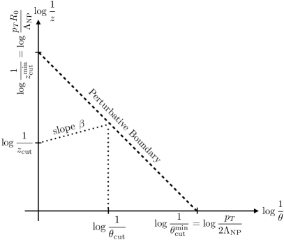
To enforce that an emission is perturbative, we require that the relative $k_{t}$ of the emission is larger than a perturbative cutoff scale $\Lambda_{\text{NP}}$, i.e.

$$z\,\theta\gtrsim\frac{\Lambda_{\text{NP}}}{p_{T}}\,,$$ (27)

where $z$ and $\theta$ are the energy fraction and splitting angle of the emission, and $p_{T}$ is the transverse momentum of the jet. Below, we take $\Lambda_{\text{NP}}=2$ GeV unless otherwise noted. For an emission that just passes soft drop, and therefore contributes to the soft drop multiplicity, we have

$$z\gtrsim{z_{\text{cut}}}\frac{\theta^{\beta}}{R_{0}^{\beta}}\,.$$ (28)

There are two regimes to consider. For $\beta>-1$ as in Fig. 8a, we can find the intersection of Eqs. (27) and (28). Setting $\theta\to{\theta_{\text{cut}}}$, we find a restriction on ${\theta_{\text{cut}}}$ to be perturbative:

$${\theta_{\text{cut}}}\gtrsim\left(\frac{\Lambda_{\text{NP}}}{{z_{\text{cut}}}p_{T}R_{0}}\right)^{\frac{1}{1+\beta}}R_{0}\,.$$ (29)

To determine the optimal choice of ${z_{\text{cut}}}$ while enforcing perturbativity, we set ${\theta_{\text{cut}}}$ to saturate this inequality and insert it into the double-log expression for the average soft drop multiplicity, Eq. (21). Maximizing this quantity, we find the optimal ISD parameters to be

$$\quad\left.{z_{\text{cut}}}\right|_{\text{optimal}} =\frac{1}{2}\left(\frac{2\Lambda_{\text{NP}}}{p_{T}R_{0}}\right)^{\frac{1}{2+\beta}}\,,$$ (30)

$$\quad\left.{\theta_{\text{cut}}}\right|_{\text{optimal}} =\left(\frac{2\Lambda_{\text{NP}}}{p_{T}R_{0}}\right)^{\frac{1}{2+\beta}}R_{0}\,.$$ (31)

The factors of two arise because the energy fraction of the softer emission is (by definition) less than $1/2$. Inserting these results into the expression for the average soft drop multiplicity, we find the largest perturbative value for the mean soft drop multiplicity to be

$$\quad\langle n_{\text{SD}}\rangle^{\beta>-1}_{\text{optimal}}\simeq\frac{\alpha_{s}}{\pi}\frac{C_{i}}{2+\beta}\log^{2}\left(\frac{2\Lambda_{\text{NP}}}{p_{T}R_{0}}\right)\,.$$ (32)

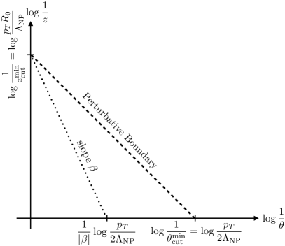
For $\beta<-1$, one can see from the $(\log 1/\theta,\log 1/z)$ phase space in Fig. 8b that an angular cutoff is not needed to avoid the nonperturbative region, so we can set ${\theta_{\text{cut}}}=0$. In this case, ${z_{\text{cut}}}$ saturates the bound Eq. (27) for $\theta\to R_{0}$, yielding

$$\left.{z_{\text{cut}}}\right|_{\text{optimal}}=\frac{\Lambda_{\text{NP}}}{p_{T}R_{0}},$$ (33)

and the average soft drop multiplicity is

$$\langle n_{\text{SD}}\rangle^{\beta<-1}_{\text{optimal}}\simeq\frac{\alpha_{s}}{\pi}\frac{C_{i}}{|\beta|}\log^{2}\left(\frac{2\Lambda_{\text{NP}}}{p_{T}R_{0}}\right)\,.$$ (34)

Combining these regions for all $\beta\in(-\infty,\infty)$, the maximum attainable mean soft drop multiplicity with perturbative parameters is

$$\langle n_{\text{SD}}\rangle_{\text{optimal}}\simeq\frac{\alpha_{s}C_{i}}{\pi}\min\left[\frac{1}{|\beta|},\frac{1}{|2+\beta|}\right]\log^{2}\left(\frac{2\Lambda_{\text{NP}}}{p_{T}R_{0}}\right)\,.$$ (35)

In particular, the mean is maximized for $\beta=-1$, giving the optimal perturbative discrimination power in this double-log approximation. This result can be understood directly from Fig. 8, which shows that soft drop multiplicity with $\beta=-1$ can capture all of the perturbative emissions in phase space.

(a)

(b)

Figure 9: (a) Discrimination power of soft drop multiplicity as a function of $\beta$, with the optimal (perturbative) values of ${z_{\text{cut}}}$ and ${\theta_{\text{cut}}}$ computed from Eqs. (30), (31), and (33) using $\Lambda_{\text{NP}}=2$ GeV. (b) Ratio of mean $n_{\text{SD}}$ as a function of $\beta$ to mean $n_{\text{SD}}$ at $\beta=0$. The Vincia results for quarks and gluons agree with the double log prediction from Eq. (35), except near $\beta=-1$ where nonperturbative effects become important.

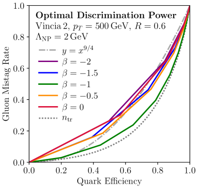
We can directly test this double-log prediction in parton shower generators. In Fig. 9a, we show the quark/gluon ROC curve for soft drop multiplicity with the optimal perturbative soft drop parameters, sweeping through $\beta$. The best discrimination power found in Vincia is indeed observed near $\beta=-1$. For a more quantitative test, Eq. (35) predicts that the ratio of the optimal soft drop multiplicity for a given value of $\beta$ to the optimal soft drop multiplicity at $\beta=0$ is

$$\frac{\langle n_{\text{SD}}\rangle_{\text{optimal}}}{\langle n_{\text{SD}}\rangle^{\beta=0}_{\text{optimal}}}=\min\left[\frac{2}{|\beta|},\frac{2}{|2+\beta|}\right]\,.$$ (36)

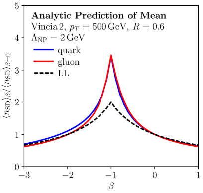
In Fig. 9b, we compare this ratio to distributions extracted from Vincia and find good agreement away from $\beta=-1$. Note that when $\beta=-1$, the counted and nonperturbative regions share a boundary, while in all other cases the two regions only meet at a single point. This explains why nonperturbative sensitivity should be amplified when $\beta$ nears $-1$. This extra sensitivity could of course be mitigated by using a more conservative value of $\Lambda_{\text{NP}}$, but there is a tradeoff between reducing nonperturbative effects and increasing discrimination power.

(a)

(b)

Figure 10: (a) Discrimination power of soft drop multiplicity as a function of $\Lambda_{\text{NP}}$ with $\beta=-1$, ${\theta_{\text{cut}}}=0$, and ${z_{\text{cut}}}$ computed from Eq. (33). (b) Impact of hadronization and underlying event in Vincia on gluon distributions.

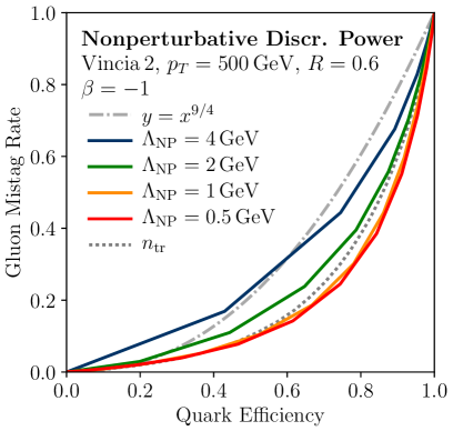
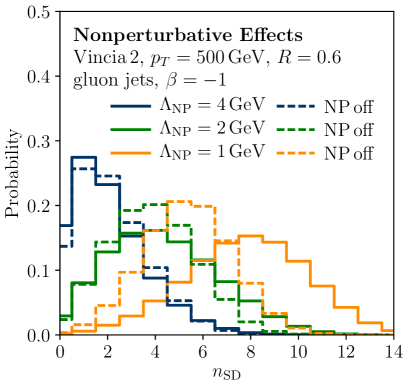
In Fig. 10a, we show the effect that decreasing $\Lambda_{\text{NP}}$ (and thus decreasing ${z_{\text{cut}}}$ and ${\theta_{\text{cut}}}$) has on the discrimination power, holding $\beta=-1$ fixed. Note that $n_{\text{SD}}$ rivals $n_{\text{tr}}$ for $\Lambda_{\text{NP}}=1$ GeV, but that there is no gain in performance when $\Lambda_{\text{NP}}$ is taken smaller. In Fig. 10b we show the shift in gluon $n_{\text{SD}}$ distributions from switched off hadronization and underlying event in Vincia. We take this as an indicator of nonperturbative sensitivity in the distributions. One can see that perturbative control is lost for $\Lambda_{\text{NP}}<2$ GeV. For $p_{T}=500$ GeV, $\Lambda_{\text{NP}}=2$ GeV gives the benchmark parameters in Eq. (11).

Our perturbative analysis here was restricted to LL order and fixed coupling, and the inclusion of higher-order effects will affect the discrimination power of soft drop multiplicity. In particular, at NLL order, quark and gluon jet flavors can mix, so we expect that higher-order effects in general decrease the discrimination power from the LL prediction. We perform NLL calculations and compare our results to parton showers in Sec. 4. Beyond these higher-order effects, we have restricted the analysis to perturbative parameters. Allowing nonperturbative emissions to contribute to the soft drop multiplicity should improve the discrimination power, however, at the expense of loss of predictivity. We discuss in Sec. 5 how to restore some of this predictive power in the nonperturbative regime with GFFs.

One might wonder if the discrimination power could be further improved by weighting the emissions, e.g. by their energy, as in the weighted soft drop multiplicity of Eq. (12). At LL order, however, the soft drop multiplicity is provably the most powerful discriminant that can be defined on the $(z_{n},\theta_{n})$ values. To see this, note that the normalized distribution of emissions in the $(\log 1/\theta,\log 1/z)$ plane is identical for quark and gluon jets at LL order, even including running coupling effects. Therefore, once the value of $n_{\text{SD}}$ is known for a given jet, no additional discriminatory information can be gleaned from the $(z_{n},\theta_{n})$ values. Nevertheless, weighted soft drop multiplicity provides an example of a more general observable that can be effectively studied with our analytic tools; we demonstrate this in App. A.

4 Calculations for IRC-Safe Soft Drop Multiplicity

We now demonstrate that the LL predictions of the previous section can be reproduced by a set of perturbative evolution equations. These equations describes how soft drop multiplicity evolves with decreasing ${\theta_{\text{cut}}}$, similar to traditional parton evolution Altarelli:1977zs . This approach also admits a generalization to NLL, which we use to make precise predictions for comparison to parton showers.

When talking about the resummation of large logarithms at LL and NLL accuracy, we are specifically referring to factors of $\log{z_{\text{cut}}}$ and $\log{\theta_{\text{cut}}}$, not to any logarithms associated with the $n_{\text{SD}}$ observable (which is an integer). As we already saw in Eq. (21), these logarithms control the size of the emission phase space, which in turn control the expected mean value of $n_{\text{SD}}$, so their resummation is essential for predicting the distribution of $n_{\text{SD}}$.

4.1 Leading-Logarithmic Evolution Equations

We begin by analyzing the soft drop multiplicity to LL accuracy. This case is simple enough to keep the structure of the ${\theta_{\text{cut}}}$ evolution transparent; the generalization to NLL just requires keeping track of more details. To achieve LL accuracy, we need only consider soft-collinear gluons emitted from the hard core of a jet; flavor-changing effects are not present at this order. Furthermore, the trunk of the clustering tree retains all but an $\mathcal{O}({z_{\text{cut}}})$ fraction of the original jet’s energy, so for ${z_{\text{cut}}}\ll 1$, energy losses are negligible at this order as well.

Let $p_{n}^{i}({\theta_{\text{cut}}})$ denote the probability that, given a jet of flavor $i$ and ISD parameter ${\theta_{\text{cut}}}$, its soft drop multiplicity $n_{\text{SD}}({\theta_{\text{cut}}})$ is measured to be $n$. Here, we leave the dependence on ${z_{\text{cut}}}$ and $\beta$ implicit, since they do not participate directly in the evolution equations. Since $n_{\text{SD}}$ is a discrete counting observable, $p_{n}^{i}({\theta_{\text{cut}}})$ is finite and should satisfy the normalization condition $\sum_{n=0}^{\infty}p_{n}^{i}({\theta_{\text{cut}}})=1$ for each flavor $i$.

We can compute the distribution for $p_{n}^{i}({\theta_{\text{cut}}})$ by solving a set of evolution equations. Consider decreasing the resolution angle from ${\theta_{\text{cut}}}$ to ${\theta_{\text{cut}}}-\delta{\theta_{\text{cut}}}$. The value of $n_{\text{SD}}$ will increase by one if there is an emission in the interval $[{\theta_{\text{cut}}}-\delta{\theta_{\text{cut}}},{\theta_{\text{cut}}}]$ that passes soft drop; otherwise $n_{\text{SD}}$ will remain unchanged. That is,

$$p_{n}^{i}({\theta_{\text{cut}}}-\delta{\theta_{\text{cut}}}) =p_{n-1}^{i}({\theta_{\text{cut}}})\,\frac{\delta{\theta_{\text{cut}}}}{{\theta_{\text{cut}}}}\int_{0}^{1/2}\text{d}z\,{\alpha_{s}(z\,{\theta_{\text{cut}}}\,p_{T})\over\pi}\,P_{i\to i}(z)\,\Theta_{\text{SD}}(z,{\theta_{\text{cut}}})$$

$$\hskip 14.22636pt+p_{n}^{i}({\theta_{\text{cut}}})\left(1-\frac{\delta{\theta_{\text{cut}}}}{{\theta_{\text{cut}}}}\int_{0}^{1/2}\text{d}z\,{\alpha_{s}(z\,{\theta_{\text{cut}}}\,p_{T})\over\pi}\,P_{i\to i}(z)\,\Theta_{\text{SD}}(z,{\theta_{\text{cut}}})\right).$$ (37)

Here, $P_{i\to i}(z)$ is the splitting function for the hard parton $i$ to emit a collinear gluon of energy fraction $z$ (and remain as flavor $i$), and $\Theta_{\text{SD}}(z,\theta)$ imposes the soft drop condition,

$$\Theta_{\text{SD}}(z,\theta)\equiv\Theta\!\left(z-{z_{\text{cut}}}\,{\theta^{\beta}\over R_{0}^{\beta}}\right).$$ (38)

At LL, $\alpha_{s}(z\,{\theta_{\text{cut}}}\,p_{T})$ runs with the 1-loop $\beta$ function.

Using Eq. (37), we can derive the linear first-order differential equation in ${\theta_{\text{cut}}}$,

$${\text{d}p_{n}^{i}\over\text{d}{\theta_{\text{cut}}}}={p_{n}^{i}({\theta_{\text{cut}}})-p_{n-1}^{i}({\theta_{\text{cut}}})\over{\theta_{\text{cut}}}}\int_{0}^{1/2}\text{d}z\,{\alpha_{s}(z\,{\theta_{\text{cut}}}\,p_{T})\over\pi}\,P_{i\to i}(z)\,\Theta_{\text{SD}}(z,{\theta_{\text{cut}}})\,.$$ (39)

Because no emissions are recorded outside the jet radius $R_{0}$, there is a boundary condition $p_{n}^{i}(R_{0})=\delta_{n,0}$. With this boundary condition, the solution to Eq. (39) is

$$p_{0}^{i}({\theta_{\text{cut}}}) =e^{-I_{i\to i}({\theta_{\text{cut}}},R_{0})}\,,$$ (40)

$$p_{n\geq 1}^{i}({\theta_{\text{cut}}}) =\int_{\theta_{\text{cut}}}^{R_{0}}{\text{d}\theta\over\theta}~{}e^{-I_{i\to i}({\theta_{\text{cut}}},\theta)}\left(\int_{0}^{1/2}\text{d}z\,{\alpha_{s}(z\,\theta\,p_{T})\over\pi}\,P_{i\to i}(z)\,\Theta_{\text{SD}}(z,\theta)\right)\,p_{n-1}^{i}(\theta)\,,$$ (41)

where

$$I_{i\to i}(\theta_{1},\theta_{2})=\int_{\theta_{1}}^{\theta_{2}}{\text{d}\theta\over\theta}\int_{0}^{1/2}\text{d}z\,{\alpha_{s}(z\,\theta\,p_{T})\over\pi}~{}P_{i\to i}(z)\,\Theta_{\text{SD}}(z,\theta)\,.$$ (42)

The expression in Eq. (40) corresponds to the case of no emissions between $R_{0}$ and ${\theta_{\text{cut}}}$. The expression in Eq. (41) computes the probability that ISD records $n-1$ emissions in the interval $[\theta,R_{0}]$, one final emission at $\theta$, then zero emissions in the interval $[{\theta_{\text{cut}}},\theta]$, with an integral over the angle $\theta$ where the final counted emission occurs.

We can interpret Eq. (41) as a recursion relation in $n$ with Eq. (40) as the initial condition. The first step in the recursion ($n=1$) gives

$$p_{1}^{i}({\theta_{\text{cut}}}) =\int_{\theta_{\text{cut}}}^{R_{0}}{\text{d}\theta\over\theta}\,e^{-I_{i\to i}({\theta_{\text{cut}}},\theta)}\,\left(\int_{0}^{1/2}\text{d}z\,{\alpha_{s}(z\,\theta\,p_{T})\over\pi}~{}P_{i\to i}(z)\,\Theta_{\text{SD}}(z,\theta)\right)\,e^{-I_{i\to i}(\theta,R_{0})}$$

$$=e^{-I_{i\to i}({\theta_{\text{cut}}},R_{0})}I_{i\to i}({\theta_{\text{cut}}},R_{0})\,.$$ (43)

A similar simplification occurs for each value of $n$, and we recognize the Poisson distribution we found in Eq. (22):

$$p_{n}^{i}({\theta_{\text{cut}}})={1\over n!}\,\Big{[}I_{i\to i}({\theta_{\text{cut}}},R_{0})\Big{]}^{n}\,e^{-I_{i\to i}({\theta_{\text{cut}}},R_{0})}\,.$$ (44)

At LL, the soft drop multiplicity $n_{\text{SD}}$ is thus Poisson distributed with mean $\lambda_{i}=I_{i\to i}({\theta_{\text{cut}}},R_{0})$. With fixed coupling, the mean value agrees exactly with $\lambda_{i}=\rho_{i}A_{\text{emit}}$ found before (see Eqs. (15) and (21)):

$$\left.I_{i\to i}({\theta_{\text{cut}}},R_{0})\right|_{\text{fixed }\alpha_{s}}=\frac{2\alpha_{s}C_{i}}{\pi}\log\frac{R_{0}}{{\theta_{\text{cut}}}}\left(\log\frac{1}{2{z_{\text{cut}}}}+\frac{\beta}{2}\log\frac{R_{0}}{{\theta_{\text{cut}}}}\right).$$ (45)

4.2 Next-to-Leading-Logarithmic Corrections

The next-to-leading logarithms take the form $\alpha_{s}^{n}\,\log^{n}{z_{\text{cut}}}$ and $\alpha_{s}^{n}\,\log^{n}{\theta_{\text{cut}}}$ in the logarithm of $p_{n}^{i}({\theta_{\text{cut}}})$. To resum these, we must consider emitted partons that are not necessarily soft and that can be either quarks or gluons. This requires us to take energy losses and flavor changes into account at this accuracy. It is convenient to compute $p_{n}^{i}({\theta_{\text{cut}}})$ by expressing it as

$$p_{n}^{i}({\theta_{\text{cut}}})=\sum_{j=q,g}\int_{1/2^{n}}^{1}\text{d}Z\,p_{n}^{i\to j(Z)}({\theta_{\text{cut}}})\,.$$ (46)

Here, $\text{d}Z\,p_{n}^{i\to j(Z)}({\theta_{\text{cut}}})$ is the differential probability that, given a jet of flavor $i$, ISD counts $n$ emissions from its hard core that result in a flavor change from $i$ to $j$, and a remaining energy fraction in the interval $[Z,Z+\text{d}Z]$. These more differential distributions evolve with ${\theta_{\text{cut}}}$ as

$$p_{n}^{i\to j(Z)}({\theta_{\text{cut}}}-\delta{\theta_{\text{cut}}})$$

$$\hskip 14.22636pt=p_{n}^{i\to j(Z)}({\theta_{\text{cut}}})\,\left(1-{\delta{\theta_{\text{cut}}}\over{\theta_{\text{cut}}}}\int_{0}^{1/2}\text{d}z\,{\alpha_{s}(z\,{\theta_{\text{cut}}}\,Z\,p_{T})\over\pi}\,P_{j\to\text{any}}(z)\,\Theta_{\text{SD}}(z,{\theta_{\text{cut}}})\right)$$

$$\hskip 14.22636pt+\sum_{k}\,{\delta{\theta_{\text{cut}}}\over{\theta_{\text{cut}}}}\,\int_{0}^{1/2}\text{d}z\,{\alpha_{s}\big{(}z\,\theta\,{Z\over 1-z}\,p_{T}\big{)}\over\pi}\,P_{k\to j}(z)\,\Theta_{\text{SD}}(z,\theta)\,p_{n-1}^{i\to k[Z/(1-z)]}({\theta_{\text{cut}}})~{}{1\over 1-z}\,,$$ (47)

where

$$P_{i\to\text{any}}(z)=\sum_{j}P_{i\to j}(z)\,.$$ (48)

The middle line of Eq. (47) is the probability that $n$ emissions are counted at resolution ${\theta_{\text{cut}}}$, and that only virtual or soft-dropped emissions (neither of which have an impact on energy fractions, up to ${z_{\text{cut}}}$ corrections) occur in the interval $[{\theta_{\text{cut}}}-\delta{\theta_{\text{cut}}},{\theta_{\text{cut}}}]$. The second line is the probability that $n-1$ emissions are counted at resolution ${\theta_{\text{cut}}}$ and result in a flavor conversion $i\to k$, and that an additional counted emission causing further conversion $k\to j$ occurs in $[{\theta_{\text{cut}}}-\delta{\theta_{\text{cut}}},{\theta_{\text{cut}}}]$.

We now justify that these evolution equations do indeed resum large logarithms to NLL, with one caveat. As is necessary for NLL resummation, these evolution equations contain NLO information about the jet’s substructure. To achieve NLL accuracy, we need to properly include the following double-emissions structures: collinear plus collinear (C+C), soft plus collinear (S+C), soft plus soft (S+S), and hard plus soft-collinear (H+SC). Since ISD is an angular-ordered algorithm, collinear emissions factorize in the cross section, so our evolution equations correctly include C+C and S+C double emissions. The S+S case is included as well by letting $\alpha_{s}$ run with the 2-loop $\beta$ function in the CMW scheme Catani:1990rr . The one caveat is that we do not describe H+SC double emissions correctly at NLO, since we use splitting functions instead of full matrix elements. Thus, our approximation should become more accurate as the jet radius $R_{0}$ becomes smaller, forcing hard emissions in the jet to become collinear. We also ignore the effects of logarithms of ${z_{\text{cut}}}$ that arise from nonglobal radiation Dasgupta:2001sh , and so do not describe emissions in the jet from secondary radiation from outside of the jet.

Despite the extra complications at NLL order, Eq. (47) is still a linear first-order differential equation, just as in Sec. 4.1. The solution is

$$p_{0}^{i\to j(Z)}({\theta_{\text{cut}}}) =\delta_{ji}\,\delta(Z-1)\,\exp\left[-I_{i\to\text{any}}({\theta_{\text{cut}}},R_{0})\right]\,,$$ (49)

$$p_{n\geq 1}^{i\to j(Z)}({\theta_{\text{cut}}}) =\sum_{k}\,\int_{\theta_{\text{cut}}}^{R_{0}}{\text{d}\theta\over\theta}\int_{0}^{1/2}\text{d}z\,\exp\left[-I_{j(Z)\to\text{any}}({\theta_{\text{cut}}},\theta)\right]$$

$$\hskip 14.22636pt\times{\alpha_{s}\big{(}z\,\theta\,{Z\over 1-z}\,p_{T}\big{)}\over\pi}\,P_{k\to j}(z)\,\Theta_{\text{SD}}(z,\theta)\,p_{n-1}^{i\to k[Z/(1-z)]}(\theta)~{}{1\over 1-z},$$ (50)

where

$$I_{j(Z)\to\text{any}}(\theta_{1},\theta_{2})=\int_{\theta_{1}}^{\theta_{2}}{\text{d}\theta\over\theta}\int_{0}^{1/2}\text{d}z\,{\alpha_{s}(z\,\theta\,Z\,p_{T})\over\pi}~{}P_{j\to\text{any}}(z)\,\Theta_{\text{SD}}(z,\theta)\,.$$ (51)

Note that $p_{n}^{i\to j(Z)}$ vanishes for $Z<1/2^{n}$. The same manipulations that led to Eq. (43) and the Poisson distribution at LL do not go through at NLL, so we cannot write $p_{n}^{i\to j(Z)}$ or $p_{n}^{i}$ in closed form at this order. Nonetheless, the integrals in Eq. (50) can be performed numerically by first computing $p_{1}^{i\to j(Z)}({\theta_{\text{cut}}})$, then computing $p_{2}^{i\to j(Z)}({\theta_{\text{cut}}})$, and so on until $p_{n}^{j}$ is negligible. In practice, the probability saturates for $n$ of order 10.

(a)

(b)

(c)

(d)

Figure 11: Calculations at LL and NLL accuracy for (left column) $n_{\text{SD}}$ distributions and (right column) the corresponding quark/gluon ROC curves. Parameters are chosen according to Eqs. (30), (31), and (33) with $\Lambda_{\text{NP}}=2$ GeV and (top row) $\beta=-1$ and (bottom row) $\beta=-0.5$. The uncertainties in the NLL calculation come from varying the $\alpha_{s}$ scale by a factor of 2.

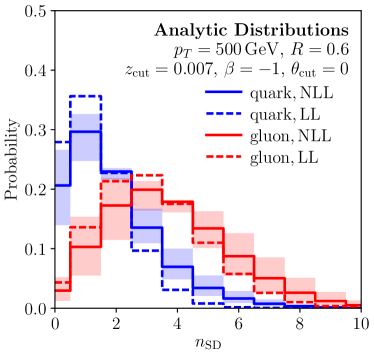
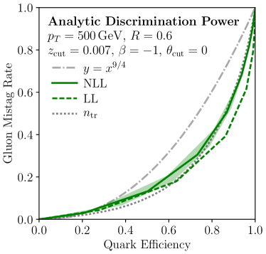
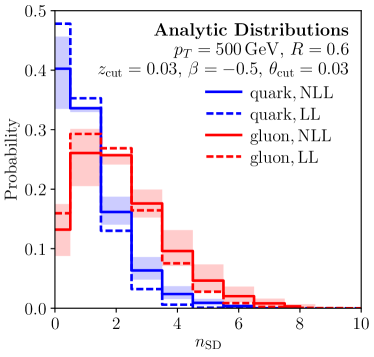
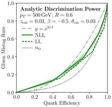
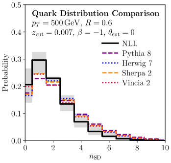
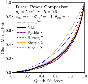
The $n_{\text{SD}}$ distributions and ROC curves at LL and NLL accuracy are displayed in Fig. 11. The uncertainties in the NLL calculation come from varying the $\alpha_{s}$ scale up and down by a factor of 2. (Scale variation in the LL calculation does not give a reliable estimate of the uncertainty, since flavor-changing processes are absent at LL; we therefore omit bands around the LL predictions.) The fact that the uncertainties are abnormally small in one bin is an artifact of this one-dimensional variation procedure, which leaves the scale-varied distributions properly normalized. Also, the uncertainties in the ROC curve are substantially smaller than the uncertainties in the NLL distributions, since the way we implement the scale variation affects quarks and gluons in a correlated way. We show both $\beta=-1$ and $\beta=-0.5$ with ${z_{\text{cut}}}$ and ${\theta_{\text{cut}}}$ chosen to be “optimal” according to Eqs. (30), (31), and (33) with $\Lambda_{\text{NP}}=2$ GeV. One can see that NLL corrections result in a slight decrease in discrimination power compared to LL, due in part to the flavor changes that occur at this order.

4.3 Comparison to Parton Showers

It is instructive to compare our NLL calculation of the soft drop multiplicity $n_{\text{SD}}$ with results obtained from parton shower generators. In addition to the Vincia setup described in Sec. 2.1, we obtained alternative event samples by showering the hard events through Pythia 8.219 Sjostrand:2006za ; Sjostrand:2014zea , Herwig 7.0.1 Bahr:2008pv ; Bellm:2015jjp , and Sherpa 2.2.0 Gleisberg:2008ta , interfaced to their default hadronization and underlying event models.

(a)

(b)

(c)

(d)

Figure 12: Impact of nonperturbative effects on (left column) $n_{\text{SD}}$ distributions and (right column) the corresponding ROC curves. This study employs Vincia, where parameters are chosen according to Eqs. (30), (31), and (33) with $\Lambda_{\text{NP}}=2$ GeV and (top row) $\beta=-1$ and (bottom row) $\beta=-0.5$.

(a)

(b)

(c)

(d)

Figure 13: Predicted quark/gluon discrimination power from (a) Pythia 8.219, (b) Herwig 7.0.1, (c) Sherpa 2.2.0, and (d) Vincia 2.0.01. While the generators disagree about absolute performance, they agree that $n_{\text{SD}}$ with $\beta=-1$ outperforms jet mass and approaches the discrimination power of $n_{\text{tr}}$.

(a)

(b)

(c)

(d)

(e)

(f)

Figure 14: Analytic NLL distributions compared to parton shower generators for (top row) quark jets, (middle row) gluon jets, along with (bottom row) the corresponding ROC curves. Parameters are chosen according to Eqs. (30), (31), and (33) with $\Lambda_{\text{NP}}=2$ GeV and (left column) $\beta=-1$ and (right column) $\beta=-0.5$.

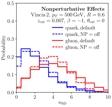
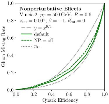
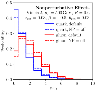
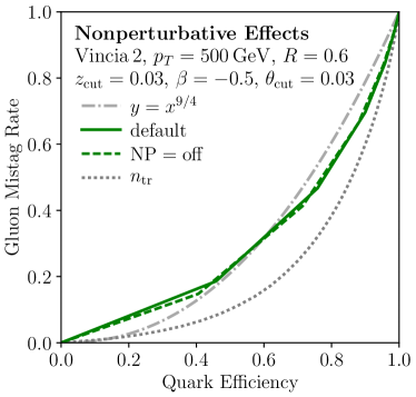
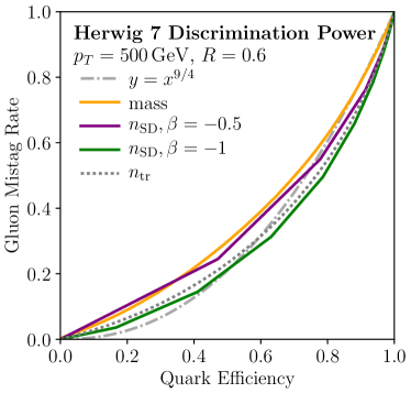
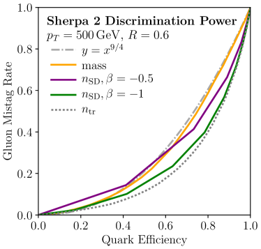
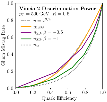
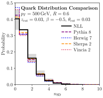
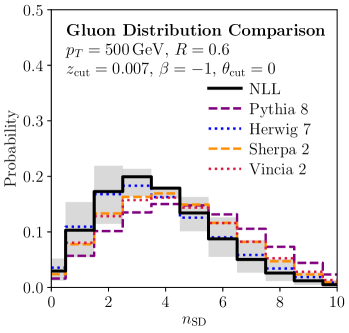
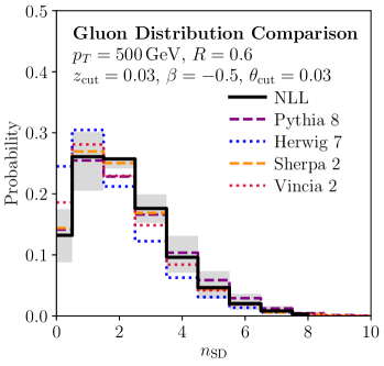
First, to validate the reliability of our NLL calculation, we want to explore the impact of nonperturbative effects on the parton showers. In Sec. 3.3 we noted that hadronization effects should generically be minimal provided parameters are chosen at or above the values given in Eqs. (30), (31), and (33). To investigate this expectation further, we check the size of nonperturbative corrections in Vincia by turning hadronization and underlying event off and comparing to results obtained using the default settings. In Fig. 12, we show $n_{\text{SD}}$ with $\beta=-1$ and $\beta=-0.5$, where in each case ${z_{\text{cut}}}$ and ${\theta_{\text{cut}}}$ are computed using Eqs. (30), (31), and (33) with $\Lambda_{\text{NP}}=2$ GeV. As expected, nonperturbative effects are under control, confirming that our perturbative NLL calculations should indeed be reliable in predicting the $n_{\text{SD}}$ distributions. Though not shown, the other three parton shower generators also exhibit comparable nonperturbative shifts.

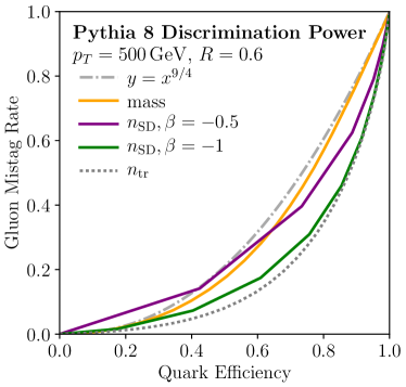
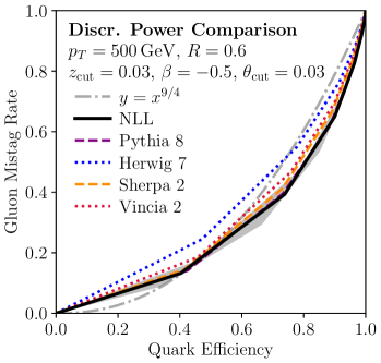
Next, we show that all parton shower generators predict that soft drop multiplicity is a relatively good quark/gluon discriminant. In Fig. 13, we compare $n_{\text{SD}}$ with $\beta=-1$ and $\beta=-0.5$ to jet mass and $n_{\text{tr}}$ for each generator separately. For $\beta=-1$, soft drop multiplicity provides a significant improvement over generic additive observables but does not quite match the performance of track multiplicity. (See, however, Fig. 10a where nonperturbative parameter values push the performance of $n_{\text{SD}}$ to match $n_{\text{tr}}$.) The ordering of the ROC curves is roughly the same between the four generators, though the absolute discrimination power does differ.

Finally, we can directly compare our NLL predictions to the parton shower generators. In Fig. 14, we show the $n_{\text{SD}}$ distributions and ROC curves for both $\beta=-1$ and $\beta=-0.5$. When interpreting these curves, one has to remember that the NLL prediction does not include nonperturbative effects. The quark distributions are roughly similar between the various generators, but there is a larger spread in the gluon distributions, a feature also seen in the study of Refs. Badger:2016bpw ; Gras:2017jty . It is interesting to note that both Vincia and Sherpa, as well as our NLL calculation, predict rather strong discrimination power, in better agreement with Pythia than with Herwig. This highlights the importance of carrying out these analytic calculations to even higher accuracy, in order to better understand the desired behavior for these parton shower generators.

5 Calculations for Collinear-Unsafe Soft Drop Multiplicity

Thus far, we have focused on choices of ISD parameters where the quark/gluon discrimination power could be predicted using perturbation theory. In the section, we consider the special case of ${\theta_{\text{cut}}}=0$ and $\beta=0$, where the soft drop multiplicity is collinear unsafe but still soft safe, allowing us to calculate its RG evolution.

5.1 Review of Generalized Fragmentation Functions

To study observables with purely collinear final-state divergences, one can use the formalism of GFFs. Ordinary fragmentation functions are well-known objects in QCD which describe the fragmentation of a quark or gluon into a single hadron. GFFs are nonperturbative objects that describe the fragmentation of a quark or gluon into correlated sets of hadrons. The GFF technique has already been applied successfully to weighted jet charge Krohn:2012fg ; Waalewijn:2012sv , track functions Chang:2013rca ; Chang:2013iba , and generalized angularities Larkoski:2014pca , and a forthcoming paper explores the broader space of observables described by GFFs Elder:2017bkd .

Each collinear-unsafe observable $x$ has an associated set of GFFs, $\mathcal{F}_{i}(x,\mu)$, where $i$ labels each quark flavor, anti-quark flavor, and gluon. They are normalized to have unit integral,

$$\int_{-\infty}^{\infty}\text{d}x\,\mathcal{F}_{i}(x,\mu)=1,$$ (52)

and at leading order, they have the interpretation of the probability of parton $i$ to yield the observable value $x$. In higher-order partonic calculations, the GFFs absorb collinear divergences and pick up dependence on the RG scale $\mu$. While the GFFs themselves cannot be calculated using perturbation theory, their RG evolution is calculable. Ordinary fragmentation functions exhibit linear DGLAP evolution Altarelli:1977zs ; Gribov:1972ri ; Dokshitzer:1977sg , whereas GFFs in general have non-linear evolution equations which can even involve mixing between different sets of GFFs.

As shown in Ref. Elder:2017bkd , though, for observables defined on a pairwise clustering tree, the evolution equations for the GFFs greatly simplify. These observables are called fractal jet observables, since their RG evolution is reminiscent of the fractal structure of the parton shower. For ${\theta_{\text{cut}}}=0$ and $\beta=0$, soft drop multiplicity (and its weighted variant) is an example of a fractal jet observable, allowing us to use the GFF formalism.

It is important to emphasize that the GFF formalism only works for purely collinear divergences. For ${\theta_{\text{cut}}}=0$ but $\beta>0$, there are mixed soft-collinear divergences in the simultaneous $z\to 0$ and $\theta\to 0$ limits. These correlated diverges would require additional regulators, similar in spirit to rapidity regularization Chiu:2012ir (see also Bertolini:2015pka ). The use of fragmentation functions to study the $\beta=0$ limit was previously considered in Ref. Larkoski:2015lea to study the soft-dropped $z_{g}$ distribution (which is the same as $z_{1}$ for ISD).

Following Ref. Elder:2017bkd , consider a fractal observable $x$ defined recursively on an IRC-safe binary clustering tree as follows. Each final-state hadron is assigned a starting weight $w_{a}$, which serves as the initial seed for the observable, and the observable $x$ is built recursively according to

$$x=\hat{x}(z,x_{1},x_{2}),$$ (53)

where $z\in[0,1]$ is the momentum fraction of the $2\to 1$ merging, and $x_{1}$ and $x_{2}$ are the values of the observable (or the starting weight $w_{a}$) on the daughter nodes. Note that $\hat{x}$ is independent of the opening angle $\theta$ of the merging, and the only angular dependence comes through the choice of clustering tree. The leading-order RG evolution for the GFFs associated with $x$ is

$$\mu\frac{\mathrm{d}}{\mathrm{d}\mu}\mathcal{F}_{i}(x,\mu)=\frac{1}{2}\sum_{jk}\int\mathrm{d}z\,\mathrm{d}x_{1}\,\mathrm{d}x_{2}\,\frac{\alpha_{s}(\mu)}{\pi}P_{i\to jk}(z)\,\mathcal{F}_{j}(x_{1},\mu)\,\mathcal{F}_{k}(x_{2},\mu)\,\delta\left[x-\hat{x}(z,x_{1},x_{2})\right],$$ (54)

where $P_{i\to jk}(z)$ is the splitting function. At this order, the evolution equation (but not the observable itself) is independent of the choice of clustering tree. Note that the evolution equation is also independent of the starting weights $w_{a}$, which are effectively encoded in the low-scale initial conditions for $\mathcal{F}_{i}$. Even though the clustering tree is IRC safe, $x$ is generally collinear unsafe, since Eq. (53) allows an exactly collinear splitting to change the observable.

The canonical RG scale for a generic GFF is

$$\mu=E_{\rm jet}R_{0},$$ (55)

and if we can extract the functional form of $\mathcal{F}_{i}(x,\mu)$ at a low scale, we can use Eq. (54) to predict their form at a higher scale. The RG equations have the same recursive structure as a parton shower, and we can use the numerical techniques of Ref. Elder:2017bkd to evolve the GFFs in $\mu$. As we will see, our observable of interest actually has a linear evolution equation, which greatly simplifies the numerical treatment.

5.2 Linear Evolution for Soft Drop Multiplicity

For ${\theta_{\text{cut}}}=0$ and $\beta=0$, soft drop multiplicity is an example of a fractal observable. More generally, any ISD observable of the form

$$x=\sum_{n}f(z_{n})$$ (56)

is a fractal observable. Using C/A for the binary clustering tree with starting weights $w_{a}=0$, the recursion relation for this general observable is

$$\hat{x}(z,x_{1},x_{2})=\begin{cases}x_{2}&\quad 0\leq z<{z_{\text{cut}}},\\ x_{2}+f(z)&\quad{z_{\text{cut}}}\leq z\leq 1/2,\\ x_{1}+f(1-z)&\quad 1/2\leq z\leq 1-{z_{\text{cut}}},\\ x_{1}&\quad 1-{z_{\text{cut}}}<z\leq 1.\end{cases}$$ (57)

The four cases check which subjet is harder and whether the softer subjet passes soft drop. If the softer subjet fails soft drop (i.e. $\min(z,1-z)<{z_{\text{cut}}}$), then the observable value is unchanged. If the softer subjet passes soft drop, then the $f(z)$ (or $f(1-z)$) value of the splitting enters linearly into the observable.

The recursion relation in Eq. (57) takes a particularly simple form, since each of the four cases involves either $x_{1}$ or $x_{2}$, but not both. This allows us to rewrite the RG evolution from Eq. (54) in the form

$$\mu\frac{\mathrm{d}}{\mathrm{d}\mu}\mathcal{F}_{i}(x,\mu)=\sum_{jk}\frac{\alpha_{s}(\mu)}{\pi}\left(\int_{0}^{{z_{\text{cut}}}}\mathrm{d}z\,P_{i\to jk}(z)\mathcal{F}_{k}(x,\mu)+\int_{{z_{\text{cut}}}}^{1/2}\mathrm{d}z\,P_{i\to jk}(z)\mathcal{F}_{k}(x-f(z),\mu)\right),$$ (58)

where we have simplified using the identity $P_{i\to jk}(z)=P_{i\to kj}(1-z)$. This evolution equation is linear, and hence is numerically no more difficult to solve than the ordinary DGLAP equations. This form holds both for the ordinary soft drop multiplicity as well as for the weighted variants in App. A, just with a different choice of $f(z)$.

5.3 Evolution for Pure Yang-Mills

Before showing numerical results, it is instructive to consider the case of $n_{f}=0$, where there is only a gluon GFF and the evolution can be studied analytically. Of course, this limit cannot teach us anything about quark/gluon discrimination directly, but we will see that the gluon GFF asymptotes to an exact Poisson distribution at sufficiently large $\mu$, such that it behaves like an idealized counting observable.

For pure Yang-Mills, we can drop flavor labels, and write the gluon GFF as $\mathcal{F}\equiv\mathcal{F}_{g}$ and the relevant splitting function as $P(z)\equiv P_{g\to gg}(z)$. Specializing to soft drop multiplicity (i.e. $f(z)=1$), the evolution equation in Eq. (58) becomes

$$\mu\frac{\mathrm{d}}{\mathrm{d}\mu}\mathcal{F}(x,\mu) =\frac{\alpha_{s}(\mu)}{\pi}\left(\int_{0}^{{z_{\text{cut}}}}\mathrm{d}z\,P(z)\mathcal{F}(x,\mu)+\int_{{z_{\text{cut}}}}^{1/2}\mathrm{d}z\,P(z)\mathcal{F}(x-1,\mu)\right)$$ (59)

$$=P_{\rm ave}\,\frac{\alpha_{s}(\mu)}{2\pi}\Bigl{(}\mathcal{F}(x-1,\mu)-\mathcal{F}(x,\mu)\Bigr{)},$$ (60)

where we have defined

$$P_{\rm ave}=\int_{z_{\rm{cut}}}^{1-z_{\rm{cut}}}\text{d}z\,P(z).$$ (61)

The interpretation of Eq. (60) is that gluon emissions that pass soft drop are added at a rate of $P_{\rm ave}\,\alpha_{s}(\mu)/2\pi$ in $\log\mu$ evolution. Specifically, in evolving from $\mu_{i}$ to $\mu_{f}$, the expected number of additional emissions is

$$\lambda(\mu_{i},\mu_{f})=\frac{P_{\rm ave}}{2\pi}\int_{\log\mu_{i}}^{\log\mu_{f}}\text{d}(\log\mu)\,\alpha_{s}(\mu),$$ (62)

so the GFF at $\mu_{f}$ is

$$\mathcal{F}(x,\mu_{f})=\mathcal{F}(x,\mu_{i})\otimes\text{Pois}(\lambda(\mu_{i},\mu_{f}))[x],$$ (63)

where the convolution is in $x$.

As $\mu_{f}$ increases, more emissions are added, so the initial GFF distributions at $\mu_{i}$ becomes less and less important. Substituting in the one-loop running of the strong coupling constant in pure Yang-Mills,

$$\alpha_{s}(\mu)=\frac{1}{\beta_{0}\log(\mu^{2}/\Lambda_{\rm QCD}^{2})},\qquad\beta_{0}=\frac{11}{3}C_{A},$$ (64)

the number of expected emissions is

$$\lambda(\mu_{i},\mu_{f})=\frac{P_{\rm ave}}{4\pi\beta_{0}}\log\left(\frac{\log\frac{\mu_{f}}{\Lambda_{\rm QCD}}}{\log\frac{\mu_{i}}{\Lambda_{\rm QCD}}}\right).$$ (65)

Since this quantity continues to grow at high $\mu_{f}$, the IR boundary condition $\mathcal{F}(x,\mu_{i})$ is irrelevant in the $\mu_{f}\to\infty$ limit, yielding the asymptotic form

$$\mathcal{F}(x,\mu\gg\Lambda_{\rm QCD})\approx\text{Pois}(\lambda(\mu))[x],\quad\lambda(\mu)=\frac{P_{\rm ave}}{4\pi\beta_{0}}\log\log\frac{\mu}{\Lambda_{\rm QCD}}.$$ (66)

Thus, we find a Poisson distribution whose mean scales as $\log\log\mu$, such that the soft drop multiplicity acts like an idealized counting observable.

5.4 Comparison to Parton Showers

(a)

(b)

(c)

(d)

Figure 15: Same as Fig. 13, but for the collinear-unsafe soft drop multiplicity with ${\theta_{\text{cut}}}=0$ and $\beta=0$.

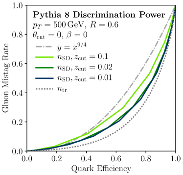
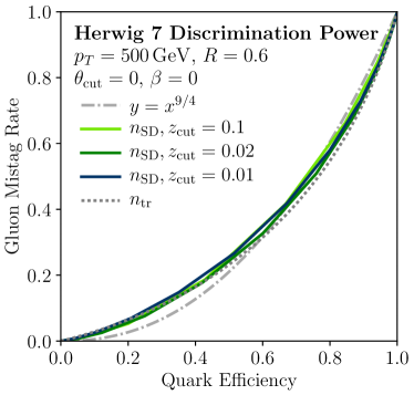
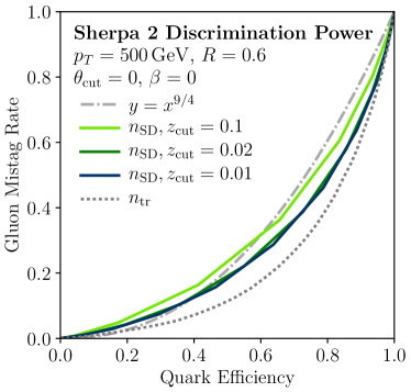
We now compare the results of the GFF approach to parton shower predictions. First, in Fig. 15, we show the predicted discrimination power for the collinear-unsafe $n_{\text{SD}}$ from the same four parton showers studied in Sec. 4.3. We see that for low ${z_{\text{cut}}}$ values, the discrimination power of the collinear-unsafe soft drop multiplicity approaches that of our benchmark IRC-safe soft drop multiplicity, previously shown in Fig. 13. (It does not, however, reach the power of the nonperturbative soft drop multiplicities shown in Fig. 10a.) Making $z_{\rm cut}$ any smaller does not significantly improve discrimination power, so we use $z_{\rm cut}=0.02$ as our baseline parameter choice.

To make a prediction using the GFF approach, we need to extract the nonperturbative distributions at a low scale and then evolve them to a higher scale. In a full analysis, the low scale distributions would be extracted from data, but here we can use the parton shower generators. For this, we switch to $e^{+}e^{-}$ collisions, generating pure quark and gluon samples through the processes $e^{+}e^{-}\to\gamma/Z^{*}\to q\bar{q}$ and $e^{+}e^{-}\to H^{*}\to gg$ in Vincia 2.0.01. Setting $R_{0}=0.6$ as our baseline, we generate jets with energies in a 10% window of $E_{\text{jet}}=400\,\mathrm{GeV}$, corresponding to $\mu=E_{\text{jet}}R_{0}=240\,\mathrm{GeV}$. We then extract $n_{\rm SD}$ from the generated events, which at leading order, is a direct measure of the corresponding GFFs.

(a)

(b)

(c)

(d)

Figure 16: RG evolution of the collinear-unsafe soft drop multiplicity for (left column) the quark singlet GFF and (right column) the gluon GFF. Shown are the results for (top row) ${z_{\text{cut}}}=0.02$ and (bottom row) ${z_{\text{cut}}}=0.1$, taking distributions extracted from Vincia at a low scale and evolving them to a higher scale. The uncertainties in the evolved distributions come from varying the jet radius used for GFF extraction and the $\mu$ scale for the RG evolution.

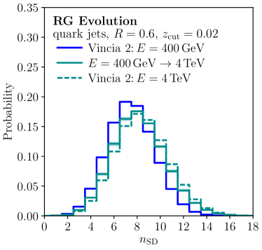
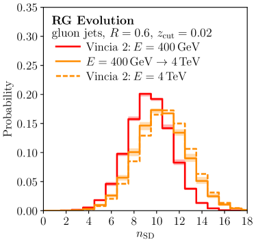
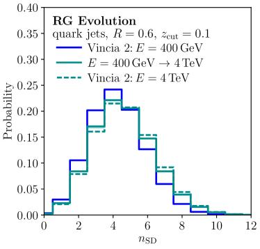
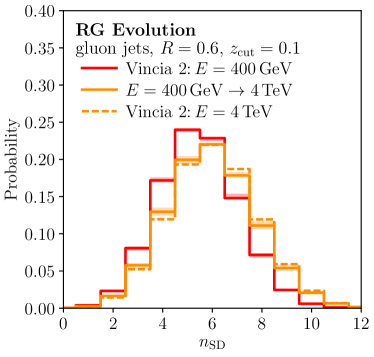
Using Eq. (58), we evolve the GFFs to $4\,\mathrm{TeV}$ using the energy scale in Eq. (55) and the two-loop running of $\alpha_{s}$. This evolution includes all 10 active quark and antiquark flavors, as $n_{f}=5$ in this energy range. There are various sources of theoretical uncertainties in the evolved result, and we highlight two of them in this study. The first contribution is due to the fact that the energy scale Eq. (55) only depends on the product $E_{\text{jet}}R_{0}$, though the initial distributions could be extracted with any $R_{0}$. To estimate this uncertainty, which serves as a consistency check of the choice of $\mu$ scale, we also extract GFFs with $R_{0}=0.3$ and $R_{0}=0.9$, keeping $\mu$ fixed. The second contribution is from uncertainty in the absolute value of the energy scale itself. To address this, we perform evolution with both half and double the energy scale of Eq. (55). We plot the envelope of these $9$ results in a shaded uncertainty band. Of course, this is only a subset of the possible GFF uncertainties, but a full study is beyond the scope of this work.

(a)

(b)

Figure 17: RG evolution of ROC curve (quark singlet vs. gluon) for the collinear-unsafe soft drop multiplicity with (a) ${z_{\text{cut}}}=0.02$ and (b) ${z_{\text{cut}}}=0.1$. In both cases, there is very little evolution in the discrimination power with energy scale.

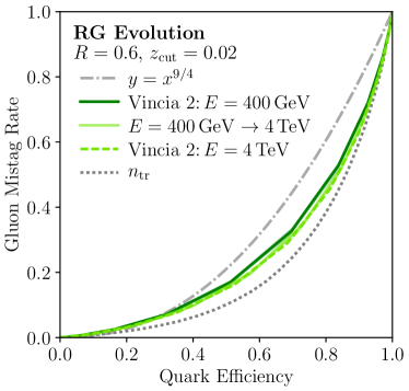
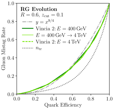
The results for ${z_{\text{cut}}}=0.02$ and ${z_{\text{cut}}}=0.1$ are shown in Fig. 16, comparing the RG-evolved results to Vincia distributions extracted at the high scale. To show a single curve for quark jets, we plot the quark-singlet distribution

$$\mathcal{Q}(x,\mu)=\frac{1}{2n_{f}}\sum_{i\in\{u,\bar{u},\ldots,b,\bar{b}\}}\mathcal{F}_{i}(x,\mu)$$ (67)

as defined in Ref. Elder:2017bkd (where it is instead denoted by $\mathcal{S}$). We find reasonable agreement between the RG evolution and Vincia for both ${z_{\text{cut}}}$ values, with a larger range of evolution for the case of ${z_{\text{cut}}}=0.02$. The uncertainties in the RG evolution do not fully cover the high-scale Vincia distribution, though it is worth emphasizing that we are only using the LO evolution equations.

In Fig. 17, we show the RG evolution of the quark/gluon ROC curves. Despite the fact that the $n_{\text{SD}}$ distributions themselves exhibit significant RG evolution, the corresponding ROC curves do not change significantly with the energy scale $\mu$. This is a key prediction of the GFF approach, and one that we can better understand by studying the moments of the GFF distributions.

5.5 Moment Space Evolution

To understand the slow evolution of the quark/gluon discrimination power, consider the evolution in moment space. Following Ref. Elder:2017bkd , the $n^{\text{th}}$ moment of a GFF is defined as

$$\overline{\mathcal{F}}_{i}(n,\mu)=\int\text{d}x\,x^{n}\mathcal{F}_{i}(x,\mu).$$ (68)

In moment space, we denote the gluon GFF by $\overline{\mathcal{G}}(n,\mu)$, and the quark-singlet GFF (as defined in Eq. (67)) by $\overline{\mathcal{Q}}(n,\mu)$. To derive the moment space evolution equations, we integrate both sides of Eq. (59) against $x^{n}$, shift the final integral by $x\to x+1$, and then simplify the $n^{\text{th}}$ moments with the splitting function identities

$$\int_{0}^{1}\mathrm{d}z\,\left[P_{g\to gg}(z)+2n_{f}P_{g\to q\bar{q}}(z)\right]=0,\quad\int_{0}^{1}\mathrm{d}z\,P_{q\to qg}(z)=0.$$ (69)

After these manipulations, the moment evolution equation for the $n^{\text{th}}$ gluon or quark-singlet GFF can be written solely in terms of the difference $\overline{\mathcal{G}}(n)-\overline{\mathcal{Q}}(n)$, along with lower moments $\overline{\mathcal{G}}(k)$, $\overline{\mathcal{Q}}(k)$ for $k<n$.

For $n=1$, the evolution equation for the means is

$$\mu\frac{\mathrm{d}}{\mathrm{d}\mu}\begin{pmatrix}\overline{\mathcal{G}}(1)\\ \overline{\mathcal{Q}}(1)\end{pmatrix}=\frac{\alpha_{s}}{\pi}\left[\big{(}\overline{\mathcal{G}}(1)-\overline{\mathcal{Q}}(1)\big{)}\begin{pmatrix}\bar{P}_{g\to gg}^{0,1/2}\\ \bar{P}_{q\to qg}^{0,1/2}\end{pmatrix}+\begin{pmatrix}\bar{P}_{g\to gg}^{{z_{\text{cut}}},1/2}+2n_{f}\bar{P}_{g\to\bar{q}q}^{{z_{\text{cut}}},1/2}\\ \bar{P}_{q\to qg}^{{z_{\text{cut}}},1/2}+\bar{P}_{q\to gq}^{{z_{\text{cut}}},1/2}\end{pmatrix}\right]$$ (70)

where we are suppressing the $\mu$ arguments and using the abbreviated notation

$$\bar{P}_{i\to jk}^{z_{1},z_{2}}=\int_{z_{1}}^{z_{2}}\mathrm{d}z\,P_{i\to jk}(z).$$ (71)

The appearance of the difference of the moments on the right-hand side has a dramatic effect on the high-energy limit of the evolution. Specifically, the difference in the means evolves as

$$\mu\frac{\mathrm{d}}{\mathrm{d}\mu}\big{(}\overline{\mathcal{G}}(1)-\overline{\mathcal{Q}}(1)\big{)}=\frac{\alpha_{s}}{\pi}\left[c_{1}-c_{2}\big{(}\overline{\mathcal{G}}(1)-\overline{\mathcal{Q}}(1)\big{)}\right],$$ (72)

where $c_{1}$ and $c_{2}$ are positive constants defined by integrals of the splitting functions. Thus, at high energies, the difference in the means asymptotes to a constant,

$$\overline{\mathcal{G}}(1)-\overline{\mathcal{Q}}(1)\Rightarrow\frac{c_{1}}{c_{2}}=\frac{\bar{P}_{g\to gg}^{{z_{\text{cut}}},1/2}+2n_{f}\bar{P}_{g\to\bar{q}q}^{{z_{\text{cut}}},1/2}-\bar{P}_{q\to qg}^{{z_{\text{cut}}},1/2}-\bar{P}_{q\to gq}^{{z_{\text{cut}}},1/2}}{\bar{P}_{q\to qg}^{0,1/2}-\bar{P}_{g\to gg}^{0,1/2}}.$$ (73)

This asymptotic behavior is strikingly different from the LL analysis of IRC-safe multiplicity in Sec. 3. In the IRC-safe case, the LL prediction is that the gluon and quark means should have a constant ratio determined by $C_{A}/C_{F}$. Here, in the collinear-unsafe case, the gluon and quark means asymptote to having a constant difference. Physically, this occurs because the RG evolution takes flavor mixing effects into account, so that at sufficiently high energies, the $n_{\text{SD}}$ distributions for quark and gluon jets become essentially the same. While we have only presented the calculation for the quark-singlet mean, it is straightforward to show that the means for each individual quark flavor behave in the same way, with differences between different quark flavors evolving to zero.

Moving to higher moments, a useful simplification occurs for the variances,

$$\sigma^{2}_{i}=\overline{\mathcal{F}}_{i}(2)-\overline{\mathcal{F}}_{i}(1)^{2}.$$ (74)

In this case, the evolution of the variances only depends on the difference of the variances and the difference of the means,

$$\mu\frac{\mathrm{d}}{\mathrm{d}\mu}\begin{pmatrix}\sigma^{2}_{\overline{\mathcal{G}}}\\ \sigma^{2}_{\overline{\mathcal{Q}}}\end{pmatrix}=\frac{\alpha_{s}}{\pi}\left[\begin{pmatrix}\bar{P}_{g\to gg}^{0,1/2}\\ \bar{P}_{q\to qg}^{0,1/2}\end{pmatrix}\Big{(}\sigma^{2}_{\overline{\mathcal{G}}}-\sigma^{2}_{\overline{\mathcal{Q}}}-\big{(}\overline{\mathcal{G}}(1)-\overline{\mathcal{Q}}(1)\big{)}^{2}\Big{)}+\begin{pmatrix}\bar{P}_{g\to gg}^{{z_{\text{cut}}},1/2}+2n_{f}\bar{P}_{g\to\bar{q}q}^{{z_{\text{cut}}},1/2}\\ \bar{P}_{q\to qg}^{{z_{\text{cut}}},1/2}+\bar{P}_{q\to gq}^{{z_{\text{cut}}},1/2}\end{pmatrix}\right].$$ (75)

At sufficiently high energies, $\overline{\mathcal{G}}(1)-\overline{\mathcal{Q}}(1)$ approaches a constant, so the evolution equation for the variances is of the same form as the evolution equation for the means. We find that, like the means, the difference of variances asymptotes to a constant,

$$\sigma^{2}_{\overline{\mathcal{G}}}-\sigma^{2}_{\overline{\mathcal{Q}}}\Rightarrow\mathrm{const}.$$ (76)

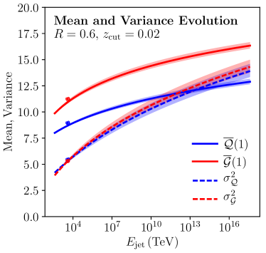
Substituting our asymptotic results back into Eq. (70) and Eq. (75), we see that both the mean and variance simply grow linearly in $\alpha_{s}(\mu)\text{d}(\log\mu)$ at high energies, so that they become proportional in the UV limit. Therefore, even with flavor-mixing effects, the soft drop multiplicity maintains a Poisson-like distribution, with $\sigma^{2}=O(\mu)$.

(a)

(b)

Figure 18: (a) RG evolution of means and variances of the quark-singlet and gluon GFFs for the soft drop multiplicity with ${z_{\text{cut}}}=0.02$. (b) RG evolution of the mean/variance differences, which asymptotically approach constants. Also shown is the relative width $w_{\mathrm{rel}}$ defined in Eq. (77), which increases slowly. For comparison, quantities extracted from Vincia at $E_{\mathrm{jet}}=4\,\mathrm{TeV}$ are shown as dots.

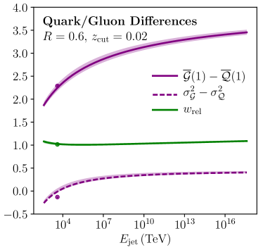
We can roughly estimate the discrimination power of the soft drop multiplicity using a relative width, similar to that of Eq. (26). Since Casimir scaling no longer holds, the distance between the quark-singlet and gluon distributions is no longer characterized by the means, but rather the difference in means. Moreover, in the UV limit, the standard deviations of the quark singlet and gluon distributions approach each other. Thus, the quantity

$$w_{\text{rel}}\equiv\frac{\sqrt{\sigma_{\overline{\mathcal{G}}}^{2}}}{\overline{\mathcal{G}}(1)-\overline{\mathcal{Q}}(1)}$$ (77)

characterizes the extent to which the distributions overlap, and hence measures the discrimination power of the soft drop multiplicity. We see that, as a result of flavor-mixing effects, the relative width is now expected to increase somewhat as more emissions are counted, roughly as the square root of the mean.

To verify these results, we numerically evolve the GFFs according to Eq. (58), starting from an initial condition extracted from Vincia 2.0.01 at $E_{\mathrm{jet}}=400\,\mathrm{GeV}$ and $R=0.6$. As in Fig. 16, we show a theoretical uncertainty band constructed from the envelope of 9 results. In Fig. 18a, we show the evolution of the mean and variance of the soft drop multiplicity for quark singlets and gluons. As expected from the above analysis, the mean and variance curves become parallel at sufficiently large values of $\mu$. This is confirmed in Fig. 18b, which shows that the differences do indeed asymptote to constant values.

Crucially, the relative width in Fig. 18b remains approximately constant over a large energy range, as the increase in the standard deviation is canceled by the increase in the mean difference as it approaches its asymptotic value. This explains the slow evolution of discrimination power seen in Fig. 17. In this way, even though these collinear-unsafe distributions cannot be predicted directly from first principles, the GFF approach gives us a valuable analytic handle on their RG evolution.

6 Conclusions

Quark/gluon discrimination has a long history, with many proposed discriminants Nilles:1980ys ; Jones:1988ay ; Fodor:1989ir ; Jones:1990rz ; Lonnblad:1990bi ; Pumplin:1991kc ; Gallicchio:2011xq ; Chatrchyan:2012sn ; Krohn:2012fg ; Larkoski:2014pca ; FerreiradeLima:2016gcz ; Komiske:2016rsd ; Davighi:2017hok though relatively few analytic calculations Larkoski:2013eya ; Larkoski:2014pca ; Bhattacherjee:2015psa . Because $C_{A}/C_{F}$ is an order 1 number, distinguishing quark- from gluon-initiated jets is an intrinsically hard problem. Moreover, to gain a quantitative understanding of quark/gluon separation power, one has to account for physics effects beyond the LL approximation, including the impact of nonperturbative physics. These physics effects are modeled to differing degrees in parton shower generators, but ultimately one wants quark/gluon studies to be based on systematically-improvable analytic calculations.

In this paper, we introduced an IRC-safe counting observable which approaches the quark/gluon discrimination performance of IRC-unsafe track multiplicity. Through a LL analysis, we demystified the power of multiplicity, showing that Poisson distributions typically yield better quark/gluon separation than Sudakov distributions, even though they are both controlled by the same $C_{A}$ and $C_{F}$ Casimir factors. Specifically, we introduced soft drop multiplicity, which depends on multiple soft gluon emissions even at LL accuracy, allowing it to outperform observables like jet mass whose value is dominated by a single gluon emission. Remarkably, there is a choice of ISD parameters where soft drop multiplicity is controlled by perturbative physics, such that its behavior can be reliably studied from first principles.

To gain a more quantitative understanding of $n_{\text{SD}}$, we introduced NLL evolution equations, which allowed us to make interesting comparisons to parton shower generators. We also studied a collinear-unsafe (but infrared-safe) version of $n_{\text{SD}}$, whose RG evolution could be studied using the formalism of GFFs. In both cases, analytic understanding was aided by the recursive structure of the observable. This motivates further studies into jet measurements performed on (groomed) clustering trees, which can depart significantly from the more commonly studied additive observables.

Ultimately, any single observable will never match the performance of multivariate jet tagging methods. This has been emphasized recently in the context of deep neural networks which exploit subtle correlations to maximize separation power Cogan:2014oua ; Almeida:2015jua ; deOliveira:2015xxd ; Baldi:2016fql ; Conway:2016caq ; Guest:2016iqz ; Barnard:2016qma ; Komiske:2016rsd ; deOliveira:2017pjk ; Kasieczka:2017nvn ; Louppe:2017ipp . Still, we are encouraged by observables like soft drop multiplicity which offer a balance between discrimination power and analytic tractability. Going beyond LL order where $n_{\text{SD}}$ can saturate the discrimination power (see Sec. 3.3), it would be interesting to study correlations between $n_{\text{SD}}$ and other IRC-safe observables like jet mass to see if there is additional information in their combination. Because the physics basis for $n_{\text{SD}}$ is so transparent, we suspect it will be a useful benchmark for both parton shower tuning and experimental jet analyses. Because the analytic structure of $n_{\text{SD}}$ is so unique, we hope it inspires new precision calculations in QCD.

Appendix A Weighted Soft Drop Multiplicity

At the end of Sec. 3, we used LL reasoning to argue that soft drop multiplicity $n_{\text{SD}}$ extracts all of the quark/gluon discriminatory information from the $(z_{n},\theta_{n})$ variables recorded by ISD. In this appendix, we study a variant of $n_{\text{SD}}$, the weighted soft drop multiplicity, defined in Eq. (12) and repeated for convenience:

$$n_{\text{SD}}^{(\kappa)}=\sum_{n}z_{n}^{\kappa}\,.$$ (78)

While quark/gluon performance is not improved by weighting, the purpose of this appendix is to demonstrate that the techniques of this paper are applicable to a variety of observables.

A.1 Discrimination Power

For small values of $\kappa$, the weighted soft drop multiplicity is still sensitive to all emissions in the region $A_{\rm emit}$. On the other hand, as $\kappa\to\infty$, only the largest $z_{n}$ value contributes significantly to the observable. As a result, the weighted multiplicity interpolates between counting and additive behavior, in the limits $\kappa\to 0$ and $\kappa\to\infty$, respectively. The $\kappa$ dependence of the discrimination power, extracted from Vincia, is shown in Fig. 19. One can see that the quark/gluon performance decreases monotonically as $\kappa$ increases.

Figure 19: Quark/gluon discrimination power of weighted soft drop multiplicity as a function of $\kappa$, at the benchmark parameters from Eq. (11). We also show the limit $\kappa\to\infty$, which is equivalent to $\max(z_{n})$.

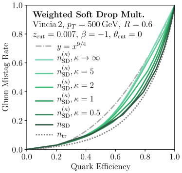
The LL distribution of the weighted soft drop multiplicity is analytically complicated. Indeed, any analytic expression for it must contain a sum of distributions, one for each value of the number $n$ of counted emissions. For example, when $\beta\leq 0$, each emission contributes at least $z_{\text{cut}}^{\kappa}$, so at most $n$ emissions can contribute to $n_{\text{SD}}^{(\kappa)}$ if its value is below $n\,z_{\text{cut}}^{\kappa}$. A full analysis along these lines is carried out in App. A.2 below.

To qualitatively understand the trend in Fig. 19, consider the limit in which ISD records many emissions. Strictly speaking, this analysis is not quantitatively applicable in the perturbative regime, where $n\lesssim 10$ emissions are counted. Nor is this reasoning applicable in the collinear-unsafe regime studied in App. A.3, where solely perturbative reasoning is insufficient. Nonetheless, the many-emission limit serves to build intuition.

In the double-logarithmic approximation, where emissions are soft and collinear and $\alpha_{s}$ is a fixed coupling, the weighted multiplicity distribution can be found from summing independent identically distributed numbers. By the central limit theorem, this converges to a normal distribution in the limit of many recorded emissions. In this limit, it suffices to compute the mean and variance of $n_{\text{SD}}^{(\kappa)}$ to estimate its discrimination power. These are determined at lowest order from the average values of $z^{\kappa}$ and $z^{2\kappa}$ in the allowed emission region as

$$\langle n_{\text{SD}}^{(\kappa)}\rangle_{i}=\rho_{i}A_{\rm emit}\langle z^{\kappa}\rangle\,,\qquad\text{Var}\left(n_{\text{SD}}^{(\kappa)}\right)_{i}=\rho_{i}A_{\rm emit}\langle z^{2\kappa}\rangle\,,$$ (79)

where

$$\langle z^{\kappa}\rangle =\frac{1}{A_{\rm emit}}\int_{{\theta_{\text{cut}}}}^{R_{0}}\frac{\text{d}\theta}{\theta}\int_{{z_{\text{cut}}}}^{1/2}\frac{\text{d}z}{z}\,z^{\kappa}\,\Theta\left[z-z_{\rm cut}\left(\frac{\theta}{R_{0}}\right)^{\beta}\right]\,.$$ (80)

With a fixed coupling, the mean value of $z^{\kappa}$ for $\beta>0$ is

$$A_{\text{emit}}\langle z^{\kappa}\rangle^{\beta>0}=\frac{1}{2^{\kappa}\kappa}\log\frac{R_{0}}{{\theta_{\text{cut}}}}-\frac{{z_{\text{cut}}}^{\kappa}}{\beta\kappa^{2}}\left(1-\left(\frac{{\theta_{\text{cut}}}}{R_{0}}\right)^{\beta\kappa}\right)\,.$$ (81)

For $\beta<0$, the mean value is

$$A_{\text{emit}}\langle z^{\kappa}\rangle^{\beta<0} =\Theta\left[{\theta_{\text{cut}}}-(2{z_{\text{cut}}})^{\frac{1}{|\beta|}}R_{0}\right]\left(\frac{1}{2^{\kappa}\kappa}\log\frac{R_{0}}{{\theta_{\text{cut}}}}-\frac{{z_{\text{cut}}}^{\kappa}}{\beta\kappa^{2}}\left[1-\left(\frac{{\theta_{\text{cut}}}}{R_{0}}\right)^{\beta\kappa}\right]\right)$$ (82)

$$\hskip 28.45274pt+\Theta\left[(2{z_{\text{cut}}})^{\frac{1}{|\beta|}}R_{0}-{\theta_{\text{cut}}}\right]\left(\frac{1}{2^{\kappa}\beta\kappa}\log(2{z_{\text{cut}}})-\frac{{z_{\text{cut}}}^{\kappa}}{\beta\kappa^{2}}\Big{[}1-(2{z_{\text{cut}}})^{-\kappa}\Big{]}\right)\,.$$

Because of the $\rho_{i}$ prefactor in Eq. (79), we see that the mean and variance once again satisfy Casimir scaling as in Eq. (24). Moreover, both the variance and mean scale with the counted area $A_{\rm emit}$, establishing that the weighted soft drop multiplicity is Poisson-like distributed as defined in Sec. 3.

The discrimination power is determined by the relative width

$$w_{\text{rel}}\equiv\frac{\sqrt{\text{Var}\left(n_{\text{SD}}^{(\kappa)}\right)_{i}}}{\left\langle n_{\text{SD}}^{(\kappa)}\right\rangle_{i}}=\frac{1}{\sqrt{\rho_{i}A_{\rm emit}}}\frac{\sqrt{\langle z^{2\kappa}\rangle}}{\langle z^{\kappa}\rangle}.$$ (83)

We can get a sense for the behavior of $w_{\text{rel}}$ by considering two extreme limits. For $\kappa\to 0$ and any choice of $\beta$, the mean value $\langle z^{\kappa}\rangle$ (and hence $w_{\text{rel}}$) approaches a constant, independent of $\kappa$. For $\kappa\to\infty$, the mean value scales with $\kappa$ like

$$A_{\text{emit}}\langle z^{\kappa}\rangle^{\kappa\to\infty}\sim\frac{1}{2^{\kappa}\kappa}\,,$$ (84)

with ${z_{\text{cut}}}<1/2$, such that the relative width scales as

$$w_{\text{rel}}^{\kappa\to\infty}\sim\sqrt{\kappa}\,.$$ (85)

Since the relative width increases with increasing $\kappa$, this reasoning predicts that the discrimination power decreases as $\kappa$ increases. This implies the best discrimination power is attained for $\kappa=0$ (i.e. ordinary soft drop multiplicity) and decreases for higher $\kappa$. Physically, the discrimination power of $n_{\text{SD}}^{(\kappa)}$ comes from sensitivity to multiple emissions, and for higher $\kappa$, sensitivity to softer emissions is decreased. In the extreme limit of $\kappa\to\infty$, the weighted soft drop multiplicity reduces to the energy fraction of the hardest emission, $n_{\text{SD}}^{\kappa\to\infty}=\max(z_{n})$.

This qualitatively explains the trend seen in Fig. 19, i.e. that the discrimination power monotonically decreasing as $\kappa$ increases. In the limit $\kappa\to\infty$, the discrimination power reaches the universal result predicted by Casimir scaling (slightly off due to small nonperturbative corrections), as the observable $\max(z_{n})$ is determined by a Sudakov form factor.

A.2 Analytic Calculation

Using evolution equations similar to those employed in Sec. 4, we can compute the distribution of IRC-safe weighted soft drop multiplicities. We will demonstrate this here at LL for simplicity; by taking into account flavor changes and energy losses, one could obtain NLL evolution equations as in Sec. 4.2. Since $n_{\text{SD}}^{(\kappa)}$ is a continuous observable, however, significantly more computation time would be required to compute its NLL distribution, in comparison to the discrete unweighted case.

Let $p^{i}(n_{\text{SD}},{\theta_{\text{cut}}})\,\text{d}n_{\text{SD}}$ denote the differential probability that, given a flavor $i$ jet, its weighted soft drop multiplicity is measured to be $n_{\text{SD}}$. Here, we leave the ${z_{\text{cut}}}$, $\beta$, and $\kappa$ dependence implicit. Though the weighted soft drop multiplicity does not directly count emissions, it is still useful to keep track of the number of contributing emissions, using

$${p^{i}(n_{\text{SD}},{\theta_{\text{cut}}})}=\sum_{n=0}^{\infty}{p^{i}_{n}(n_{\text{SD}},{\theta_{\text{cut}}})}\,,$$ (86)

where $n$ labels the number of counted emissions as before. If we change the resolution angle from ${\theta_{\text{cut}}}$ to ${\theta_{\text{cut}}}-\delta{\theta_{\text{cut}}}$, then

$$p^{i}_{n}(n_{\text{SD}},{\theta_{\text{cut}}}-\delta{\theta_{\text{cut}}}) =p^{i}_{n}(n_{\text{SD}},{\theta_{\text{cut}}})\,\left(1-{\delta{\theta_{\text{cut}}}\over{\theta_{\text{cut}}}}\,\int_{0}^{1/2}\text{d}z\,{\alpha_{s}(z\,\theta\,p_{T})\over\pi}\,P_{i\to i}(z)\,\Theta_{\text{SD}}(z,\theta)\right)$$

$$+{\delta{\theta_{\text{cut}}}\over{\theta_{\text{cut}}}}\,\int_{0}^{1/2}\text{d}z~{}{\alpha_{s}(z\,\theta\,p_{T})\over\pi}\,P_{i\to i}(z)\,\Theta_{\text{SD}}(z,\theta)\,p^{i}_{n-1}(n_{\text{SD}}-z^{\kappa},{\theta_{\text{cut}}})\,.$$ (87)

This leads to a linear differential equation. Instead of the Poisson distribution found in Sec. 4.1, the solution in this case is differential in $n_{\text{SD}}=\sum_{i}z_{i}^{\kappa}$:

$$p^{i}_{n}(n_{\text{SD}},{\theta_{\text{cut}}})$$ (88)

$$=\frac{e^{-I_{i\to i}({\theta_{\text{cut}}},R_{0})}}{n!}\left(\,\prod_{i=1}^{n}\int_{\theta_{\text{cut}}}^{R_{0}}{d\theta_{i}\over\theta_{i}}\int_{0}^{1/2}\text{d}z_{i}\,{\alpha_{s}(z_{i}\,\theta_{i}\,p_{T})\over\pi}\,P_{i\to i}(z_{i})\,\Theta_{\text{SD}}(z_{i},\theta_{i})\right)\delta\Big{(}n_{\text{SD}}-\sum_{i=1}^{n}z_{i}^{\kappa}\Big{)}\,.$$

(a)

(b)

Figure 20: LL calculation of weighted soft drop multiplicity distributions with $\kappa=1$, compared to Vincia. The plots have two different sets of ISD parameters which were chosen to display the sharp features characteristic of $n_{\text{SD}}^{(\kappa)}$ in the perturbative regime. The curves shown are the probability distribution functions of $\log n_{\mathrm{SD}}^{(1.0)}$, so that they integrate to one in logarithmic space. The leftmost bin is an underflow bin, showing the probability that no emissions were counted by ISD, such that $n_{\text{SD}}^{(1.0)}=0$.

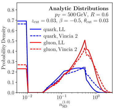
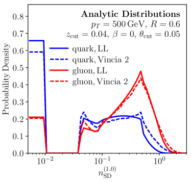
In the perturbative regime, the behavior of $n_{\text{SD}}^{(\kappa)}$ is most clearly seen on a logarithmic scale. Two example LL distributions are displayed in Fig. 20 and compared to results from Vincia. In these examples, soft drop parameters were chosen to demonstrate that the sharp features of the $n_{\text{SD}}^{(\kappa)}$ distributions are indeed captured by the LL evolution equations. These sharp features result from the edges of the $p_{n}^{i}(n_{\text{SD}},{\theta_{\text{cut}}})$ distributions for different values of $n$. For example, with $\beta\leq 0$, the $p_{n}^{i}(n_{\text{SD}},{\theta_{\text{cut}}})$ distribution only has support on the interval $[n\,z_{\text{cut}}^{\kappa},{n\over 2^{\kappa}}]$.

(a)

(b)

Figure 21: RG evolution of collinear-unsafe weighted soft drop multiplicity with ${z_{\text{cut}}}=0.01$ and $\kappa=1$, for the (a) quark-singlet and (b) gluon cases.

A.3 Collinear-Unsafe Evolution

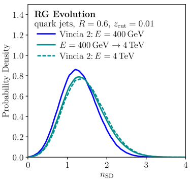
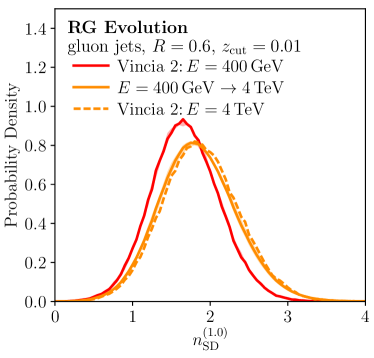
In the case of a collinear-unsafe weighted soft drop multiplicity with $\beta=0$ and $\theta_{\rm cut}=0$, we can apply the methods of Sec. 5. Specifically, after extracting the GFF at some RG scale $\mu$, we can use Eq. (58) with the particular choice $f(z)=z^{\kappa}$ to predict the upwards evolution. In Fig. 21, we compare the result of the RG evolution for ${z_{\text{cut}}}=0.01$ and $\kappa=1$ to Vincia, finding overall good agreement. By eye, one can see that these $\kappa=1$ distributions do not yield as good separation power as the $\kappa=0$ distributions shown in Fig. 16, though the degree of RG evolution is similar for both the weighted and unweighted cases.

References

- (1) ATLAS collaboration, M. Aaboud et al., Jet energy scale measurements and their systematic uncertainties in proton-proton collisions at TeV with the ATLAS detector, 1703.09665.
- (2) CMS collaboration, V. Khachatryan et al., Jet energy scale and resolution in the CMS experiment in pp collisions at 8 TeV, JINST 12 (2017) P02014, [1607.03663].
- (3) M. Dasgupta, A. Fregoso, S. Marzani and G. P. Salam, Towards an understanding of jet substructure, JHEP 09 (2013) 029, [1307.0007].
- (4) C. Frye, A. J. Larkoski, M. D. Schwartz and K. Yan, Factorization for groomed jet substructure beyond the next-to-leading logarithm, JHEP 07 (2016) 064, [1603.09338].
- (5) A. J. Larkoski and J. Thaler, Unsafe but Calculable: Ratios of Angularities in Perturbative QCD, JHEP 09 (2013) 137, [1307.1699].
- (6) M. Dasgupta, L. Schunk and G. Soyez, Jet shapes for boosted jet two-prong decays from first-principles, JHEP 04 (2016) 166, [1512.00516].
- (7) M. Dasgupta, F. Dreyer, G. P. Salam and G. Soyez, Small-radius jets to all orders in QCD, JHEP 04 (2015) 039, [1411.5182].
- (8) A. J. Larkoski, I. Moult and D. Neill, Analytic Boosted Boson Discrimination, JHEP 05 (2016) 117, [1507.03018].
- (9) M. Procura, W. J. Waalewijn and L. Zeune, Resummation of Double-Differential Cross Sections and Fully-Unintegrated Parton Distribution Functions, JHEP 02 (2015) 117, [1410.6483].
- (10) W. J. Waalewijn, Calculating the Charge of a Jet, Phys. Rev. D86 (2012) 094030, [1209.3019].
- (11) D. Adams et al., Towards an Understanding of the Correlations in Jet Substructure, Eur. Phys. J. C75 (2015) 409, [1504.00679].
- (12) A. Altheimer et al., Boosted objects and jet substructure at the LHC. Report of BOOST2012, held at IFIC Valencia, 23rd-27th of July 2012, Eur. Phys. J. C74 (2014) 2792, [1311.2708].
- (13) A. Altheimer et al., Jet Substructure at the Tevatron and LHC: New results, new tools, new benchmarks, J. Phys. G39 (2012) 063001, [1201.0008].
- (14) A. Abdesselam et al., Boosted objects: A Probe of beyond the Standard Model physics, Eur. Phys. J. C71 (2011) 1661, [1012.5412].
- (15) J. Gallicchio and M. D. Schwartz, Quark and Gluon Tagging at the LHC, Phys. Rev. Lett. 107 (2011) 172001, [1106.3076].
- (16) J. Gallicchio and M. D. Schwartz, Quark and Gluon Jet Substructure, JHEP 04 (2013) 090, [1211.7038].
- (17) A. J. Larkoski, G. P. Salam and J. Thaler, Energy Correlation Functions for Jet Substructure, JHEP 06 (2013) 108, [1305.0007].
- (18) A. J. Larkoski, J. Thaler and W. J. Waalewijn, Gaining (Mutual) Information about Quark/Gluon Discrimination, JHEP 11 (2014) 129, [1408.3122].
- (19) B. Bhattacherjee, S. Mukhopadhyay, M. M. Nojiri, Y. Sakaki and B. R. Webber, Associated jet and subjet rates in light-quark and gluon jet discrimination, JHEP 04 (2015) 131, [1501.04794].
- (20) J. R. Andersen et al., Les Houches 2015: Physics at TeV Colliders Standard Model Working Group Report, in 9th Les Houches Workshop on Physics at TeV Colliders (PhysTeV 2015) Les Houches, France, June 1-19, 2015, 2016. 1605.04692.
- (21) P. T. Komiske, E. M. Metodiev and M. D. Schwartz, Deep learning in color: towards automated quark/gluon jet discrimination, JHEP 01 (2017) 110, [1612.01551].
- (22) J. Davighi and P. Harris, Fractal based observables to probe jet substructure of quarks and gluons, 1703.00914.
- (23) P. Gras, S. Hoeche, D. Kar, A. Larkoski, L. Lönnblad, S. Plätzer et al., Systematics of quark/gluon tagging, 1704.03878.
- (24) CMS collaboration, Performance of quark/gluon discrimination in 8 TeV pp data, Tech. Rep. CMS-PAS-JME-13-002, 2013.
- (25) D. Ferreira de Lima, P. Petrov, D. Soper and M. Spannowsky, Quark-Gluon tagging with Shower Deconstruction: Unearthing dark matter and Higgs couplings, Phys. Rev. D95 (2017) 034001, [1607.06031].
- (26) B. Bhattacherjee, S. Mukhopadhyay, M. M. Nojiri, Y. Sakaki and B. R. Webber, Quark-gluon discrimination in the search for gluino pair production at the LHC, JHEP 01 (2017) 044, [1609.08781].
- (27) ATLAS collaboration, G. Aad et al., Light-quark and gluon jet discrimination in collisions at with the ATLAS detector, Eur. Phys. J. C74 (2014) 3023, [1405.6583].
- (28) ATLAS collaboration, T. A. collaboration, Discrimination of Light Quark and Gluon Jets in collisions at TeV with the ATLAS Detector, .
- (29) ATLAS collaboration, G. Aad et al., Measurement of the charged-particle multiplicity inside jets from TeV collisions with the ATLAS detector, Eur. Phys. J. C76 (2016) 322, [1602.00988].
- (30) P. Bolzoni, B. A. Kniehl and A. V. Kotikov, Gluon and quark jet multiplicities at N3LO+NNLL, Phys. Rev. Lett. 109 (2012) 242002, [1209.5914].
- (31) P. Bolzoni, B. A. Kniehl and A. V. Kotikov, Average gluon and quark jet multiplicities at higher orders, Nucl. Phys. B875 (2013) 18–44, [1305.6017].
- (32) R. K. Ellis, W. J. Stirling and B. R. Webber, QCD and collider physics, Camb. Monogr. Part. Phys. Nucl. Phys. Cosmol. 8 (1996) 1–435.
- (33) A. Banfi, G. P. Salam and G. Zanderighi, Principles of general final-state resummation and automated implementation, JHEP 03 (2005) 073, [hep-ph/0407286].
- (34) S. D. Ellis, C. K. Vermilion, J. R. Walsh, A. Hornig and C. Lee, Jet Shapes and Jet Algorithms in SCET, JHEP 11 (2010) 101, [1001.0014].
- (35) A. J. Larkoski, D. Neill and J. Thaler, Jet Shapes with the Broadening Axis, JHEP 04 (2014) 017, [1401.2158].
- (36) E. Gerwick, T. Plehn, S. Schumann and P. Schichtel, Scaling Patterns for QCD Jets, JHEP 10 (2012) 162, [1208.3676].
- (37) Z. Bern, L. J. Dixon, F. Febres Cordero, S. Hˆche, H. Ita, D. A. Kosower et al., Next-to-Leading Order -Jet Production at the LHC, Phys. Rev. D88 (2013) 014025, [1304.1253].
- (38) S. Badger, B. Biedermann, P. Uwer and V. Yundin, Next-to-leading order QCD corrections to five jet production at the LHC, Phys. Rev. D89 (2014) 034019, [1309.6585].
- (39) ATLAS collaboration, G. Aad et al., Measurements of the W production cross sections in association with jets with the ATLAS detector, Eur. Phys. J. C75 (2015) 82, [1409.8639].
- (40) A. J. Larkoski, S. Marzani, G. Soyez and J. Thaler, Soft Drop, JHEP 05 (2014) 146, [1402.2657].
- (41) Y. L. Dokshitzer, G. D. Leder, S. Moretti and B. R. Webber, Better jet clustering algorithms, JHEP 08 (1997) 001, [hep-ph/9707323].
- (42) M. Wobisch and T. Wengler, Hadronization corrections to jet cross-sections in deep inelastic scattering, in Monte Carlo generators for HERA physics. Proceedings, Workshop, Hamburg, Germany, 1998-1999, pp. 270–279, 1998. hep-ph/9907280.
- (43) ATLAS collaboration, G. Aad et al., Identification of boosted, hadronically decaying W bosons and comparisons with ATLAS data taken at TeV, Eur. Phys. J. C76 (2016) 154, [1510.05821].
- (44) M. Dasgupta, A. Fregoso, S. Marzani and A. Powling, Jet substructure with analytical methods, Eur. Phys. J. C73 (2013) 2623, [1307.0013].
- (45) B. T. Elder, M. Procura, J. Thaler, W. J. Waalewijn and K. Zhou, Generalized Fragmentation Functions for Fractal Jet Observables, 1704.05456.
- (46) W. T. Giele, D. A. Kosower and P. Z. Skands, A simple shower and matching algorithm, Phys. Rev. D78 (2008) 014026, [0707.3652].
- (47) W. T. Giele, D. A. Kosower and P. Z. Skands, Higher-Order Corrections to Timelike Jets, Phys. Rev. D84 (2011) 054003, [1102.2126].
- (48) T. Sjostrand, S. Mrenna and P. Z. Skands, A Brief Introduction to PYTHIA 8.1, Comput. Phys. Commun. 178 (2008) 852–867, [0710.3820].
- (49) M. Cacciari, G. P. Salam and G. Soyez, The Anti-k(t) jet clustering algorithm, JHEP 04 (2008) 063, [0802.1189].
- (50) M. Cacciari, G. P. Salam and G. Soyez, FastJet User Manual, Eur. Phys. J. C72 (2012) 1896, [1111.6097].
- (51) “Fastjet contrib.” http://fastjet.hepforge.org/contrib/.
- (52) H.-M. Chang, M. Procura, J. Thaler and W. J. Waalewijn, Calculating Track-Based Observables for the LHC, Phys. Rev. Lett. 111 (2013) 102002, [1303.6637].
- (53) H.-M. Chang, M. Procura, J. Thaler and W. J. Waalewijn, Calculating Track Thrust with Track Functions, Phys. Rev. D88 (2013) 034030, [1306.6630].
- (54) L. Clavelli, Jet Invariant Mass in Quantum Chromodynamics, Phys. Lett. B85 (1979) 111–114.
- (55) S. Catani, G. Turnock and B. R. Webber, Heavy jet mass distribution in e+ e- annihilation, Phys. Lett. B272 (1991) 368–372.
- (56) S. Catani, L. Trentadue, G. Turnock and B. R. Webber, Resummation of large logarithms in e+ e- event shape distributions, Nucl. Phys. B407 (1993) 3–42.
- (57) J. Gallicchio, J. Huth, M. Kagan, M. D. Schwartz, K. Black and B. Tweedie, Multivariate discrimination and the Higgs + W/Z search, JHEP 04 (2011) 069, [1010.3698].
- (58) C. F. Berger, T. Kucs and G. F. Sterman, Event shape / energy flow correlations, Phys. Rev. D68 (2003) 014012, [hep-ph/0303051].
- (59) L. G. Almeida, S. J. Lee, G. Perez, G. F. Sterman, I. Sung and J. Virzi, Substructure of high- Jets at the LHC, Phys. Rev. D79 (2009) 074017, [0807.0234].
- (60) B. Andersson, G. Gustafson, L. Lonnblad and U. Pettersson, Coherence Effects in Deep Inelastic Scattering, Z. Phys. C43 (1989) 625.
- (61) J. G. M. Gatheral, Exponentiation of Eikonal Cross-sections in Nonabelian Gauge Theories, Phys. Lett. B133 (1983) 90–94.
- (62) T. Becher and M. Neubert, On the Structure of Infrared Singularities of Gauge-Theory Amplitudes, JHEP 06 (2009) 081, [0903.1126].
- (63) S. Moch, J. A. M. Vermaseren and A. Vogt, The Three loop splitting functions in QCD: The Nonsinglet case, Nucl. Phys. B688 (2004) 101–134, [hep-ph/0403192].
- (64) J. Frenkel and J. C. Taylor, NONABELIAN EIKONAL EXPONENTIATION, Nucl. Phys. B246 (1984) 231–245.
- (65) G. Altarelli and G. Parisi, Asymptotic Freedom in Parton Language, Nucl. Phys. B126 (1977) 298–318.
- (66) S. Catani, B. R. Webber and G. Marchesini, QCD coherent branching and semiinclusive processes at large x, Nucl. Phys. B349 (1991) 635–654.
- (67) M. Dasgupta and G. P. Salam, Resummation of nonglobal QCD observables, Phys. Lett. B512 (2001) 323–330, [hep-ph/0104277].
- (68) T. Sjostrand, S. Mrenna and P. Z. Skands, PYTHIA 6.4 Physics and Manual, JHEP 05 (2006) 026, [hep-ph/0603175].
- (69) T. Sjˆstrand, S. Ask, J. R. Christiansen, R. Corke, N. Desai, P. Ilten et al., An Introduction to PYTHIA 8.2, Comput. Phys. Commun. 191 (2015) 159–177, [1410.3012].
- (70) M. Bahr et al., Herwig++ Physics and Manual, Eur. Phys. J. C58 (2008) 639–707, [0803.0883].
- (71) J. Bellm et al., Herwig 7.0/Herwig++ 3.0 release note, Eur. Phys. J. C76 (2016) 196, [1512.01178].
- (72) T. Gleisberg, S. Hoeche, F. Krauss, M. Schonherr, S. Schumann, F. Siegert et al., Event generation with SHERPA 1.1, JHEP 02 (2009) 007, [0811.4622].
- (73) D. Krohn, M. D. Schwartz, T. Lin and W. J. Waalewijn, Jet Charge at the LHC, Phys. Rev. Lett. 110 (2013) 212001, [1209.2421].
- (74) V. N. Gribov and L. N. Lipatov, Deep inelastic e p scattering in perturbation theory, Sov. J. Nucl. Phys. 15 (1972) 438–450.
- (75) Y. L. Dokshitzer, Calculation of the Structure Functions for Deep Inelastic Scattering and e+ e- Annihilation by Perturbation Theory in Quantum Chromodynamics., Sov. Phys. JETP 46 (1977) 641–653.
- (76) J.-Y. Chiu, A. Jain, D. Neill and I. Z. Rothstein, A Formalism for the Systematic Treatment of Rapidity Logarithms in Quantum Field Theory, JHEP 05 (2012) 084, [1202.0814].
- (77) D. Bertolini, J. Thaler and J. R. Walsh, The First Calculation of Fractional Jets, JHEP 05 (2015) 008, [1501.01965].
- (78) A. J. Larkoski, S. Marzani and J. Thaler, Sudakov Safety in Perturbative QCD, Phys. Rev. D91 (2015) 111501, [1502.01719].
- (79) H. P. Nilles and K. H. Streng, Quark - Gluon Separation in Three Jet Events, Phys. Rev. D23 (1981) 1944.
- (80) L. M. Jones, Tests for Determining the Parton Ancestor of a Hadron Jet, Phys. Rev. D39 (1989) 2550.
- (81) Z. Fodor, How to See the Differences Between Quark and Gluon Jets, Phys. Rev. D41 (1990) 1726.
- (82) L. Jones, TOWARDS A SYSTEMATIC JET CLASSIFICATION, Phys. Rev. D42 (1990) 811–814.
- (83) L. Lonnblad, C. Peterson and T. Rognvaldsson, Finding Gluon Jets With a Neural Trigger, Phys. Rev. Lett. 65 (1990) 1321–1324.
- (84) J. Pumplin, How to tell quark jets from gluon jets, Phys. Rev. D44 (1991) 2025–2032.
- (85) CMS collaboration, S. Chatrchyan et al., Search for a Higgs boson in the decay channel to ZZ(*) to qbar l+ in collisions at TeV, JHEP 04 (2012) 036, [1202.1416].
- (86) J. Cogan, M. Kagan, E. Strauss and A. Schwarztman, Jet-Images: Computer Vision Inspired Techniques for Jet Tagging, JHEP 02 (2015) 118, [1407.5675].
- (87) L. G. Almeida, M. Backović, M. Cliche, S. J. Lee and M. Perelstein, Playing Tag with ANN: Boosted Top Identification with Pattern Recognition, JHEP 07 (2015) 086, [1501.05968].
- (88) L. de Oliveira, M. Kagan, L. Mackey, B. Nachman and A. Schwartzman, Jet-images ? deep learning edition, JHEP 07 (2016) 069, [1511.05190].
- (89) P. Baldi, K. Bauer, C. Eng, P. Sadowski and D. Whiteson, Jet Substructure Classification in High-Energy Physics with Deep Neural Networks, Phys. Rev. D93 (2016) 094034, [1603.09349].
- (90) J. S. Conway, R. Bhaskar, R. D. Erbacher and J. Pilot, Identification of High-Momentum Top Quarks, Higgs Bosons, and W and Z Bosons Using Boosted Event Shapes, Phys. Rev. D94 (2016) 094027, [1606.06859].
- (91) D. Guest, J. Collado, P. Baldi, S.-C. Hsu, G. Urban and D. Whiteson, Jet Flavor Classification in High-Energy Physics with Deep Neural Networks, Phys. Rev. D94 (2016) 112002, [1607.08633].
- (92) J. Barnard, E. N. Dawe, M. J. Dolan and N. Rajcic, Parton Shower Uncertainties in Jet Substructure Analyses with Deep Neural Networks, Phys. Rev. D95 (2017) 014018, [1609.00607].
- (93) L. de Oliveira, M. Paganini and B. Nachman, Learning Particle Physics by Example: Location-Aware Generative Adversarial Networks for Physics Synthesis, 1701.05927.
- (94) G. Kasieczka, T. Plehn, M. Russell and T. Schell, Deep-learning Top Taggers or The End of QCD?, 1701.08784.
- (95) G. Louppe, K. Cho, C. Becot and K. Cranmer, QCD-Aware Recursive Neural Networks for Jet Physics, 1702.00748.