Testing a one-dimensional prescription of dynamical shear mixing with a two-dimensional hydrodynamic simulation

Abstract

Context. The treatment of mixing processes is still one of the major uncertainties in 1D stellar evolution models. This is mostly due to the need to parametrize and approximate aspects of hydrodynamics in hydrostatic codes. In particular, the effect of hydrodynamic instabilities in rotating stars, for example, dynamical shear instability, evades consistent description.

Aims. We intend to study the accuracy of the diffusion approximation to dynamical shear in hydrostatic stellar evolution models by comparing 1D models to a first-principle hydrodynamics simulation starting from the same initial conditions.

Methods. We chose an initial model calculated with the stellar evolution code GENEC that is just at the onset of a dynamical shear instability but does not show any other instabilities (e.g., convection). This was mapped to the hydrodynamics code SLH to perform a 2D simulation in the equatorial plane. We compare the resulting profiles in the two codes and compute an effective diffusion coefficient for the hydro simulation.

Results. Shear instabilities develop in the 2D simulation in the regions predicted by linear theory to become unstable in the 1D stellar evolution model. Angular velocity and chemical composition is redistributed in the unstable region, thereby creating new unstable regions. After a period of time, the system settles in a symmetric, steady state, which is Richardson stable everywhere in the 2D simulation, whereas the instability remains for longer in the 1D model due to the limitations of the current implementation in the 1D code. A spatially resolved diffusion coefficient is extracted by comparing the initial and final profiles of mean atomic mass.

Conclusions. The presented simulation gives a first insight on hydrodynamics of shear instabilities in a real stellar environment and even allows us to directly extract an effective diffusion coefficient. We see evidence for a critical Richardson number of 0.25 as regions above this threshold remain stable for the course of the simulation.

1 Introduction

Internal mixing plays an important role in stellar evolution. Mixing takes place under several different conditions in stellar interiors, all linked with different kinds of fluid instability: convection, dynamical shear, secular shear, Rayleigh-Taylor, thermohaline, etc. (see, for example, Heger et al. 2000; Maeder et al. 2013). Rotation-induced instabilities (e. g. dynamical shear, secular shear, GSF, ABCD) have a strong impact on the evolution and structure of stars. Stellar models including prescriptions for rotation can, depending upon the initial angular velocity, exhibit significantly different structural and evolutionary characteristics to non-rotating models (see, e.g., Heger et al. 2000; Heger & Langer 2000; Hirschi et al. 2004; Ekström et al. 2012). Most predominantly, rotating models have more massive cores, higher luminosities and more efficient mass loss via winds. In massive stars, the interior structure of the carbon-oxygen core is determined in a large part by its mass and by mixing at convective boundaries (Young et al. 2005). Whether or not a star is rotating (and how fast) can, primarily by dictating the mass of the CO core and secondarily by inducing mixing within the core, alter the pre-supernova density profile of the star. A variation in density profile (not to mention the pre-supernova angular velocity profile, see, e.g., Fryer & Heger 2000) can have a marked effect on the explosion energy, explosive nucleosynthetic yield and compact remnant type (neutron star or black hole) and mass (see O’Connor & Ott 2013; Sukhbold & Woosley 2014; Ertl et al. 2016; Sukhbold et al. 2016, and references therein).

Rotation also affects the nucleosynthesis in massive stars, especially at low metallicities. Rotation-induced mixing across convectively stable layers in massive stars has been shown to be able to explain the observed enhancement of nitrogen in the early universe (see Hirschi 2007, and references therein). In the absence of additional mixing processes, the surface nitrogen abundance should scale with the metallicity of the protostellar gas. However, transport of ¹²C and ¹⁶O from the convective He-burning across the convectively stable He layer and into the H-burning shell by the secular shear instability enables a primary production of ¹⁴N by proton captures on the transported ¹²C and ¹⁶O. The same secular shear process also transports some of this ¹⁴N from the H-burning shell in which it was created back down into the convective He-burning core, where it is exposed to higher temperatures and alpha particles, resulting in the creation of ²²Ne (two alpha-captures). ²²Ne is an efficient neutron source (activated by alpha-capture; ${}^{22}\mathrm{Ne}(\alpha,n)^{25}\mathrm{Mg}$) and its rotationally induced presence in the He-core boosts the weak slow neutron-capture ($s$) process production at low metallicities (see Frischknecht et al. 2012, 2016, for more details).

Rotation and all the other processes mentioned above are intrinsically multi-dimensional due to their turbulent nature, and their implementation in one-dimensional (1D) stellar evolution codes is not straightforward and relies on many simplifications. Usually, they are each accounted for as separate diffusive processes, the diffusion coefficients of which are summed up. The number of considered instabilities and the way they are implemented in stellar evolution codes lead to significant differences between the results of various codes, particularly for the advanced evolutionary stages of massive stars (Martins & Palacios 2013).

The results of stellar evolution calculations are thus model-dependent, and while the impact of rotation is qualitatively determined, there are still free parameters and artifacts of the numerical implementations of the rotation physics (including the artificial symmetry of rotating 1D models) that prevent the 1D models from making precise quantitative predictions. A better knowledge about how chemical species and angular momentum are transported inside stars is thus a crucial step in improving the treatment of rotation in, and hence the predictive power of, stellar evolution codes.

Because of the considerable increase in computing power and the development of modern and efficient hydrodynamics codes during the past decades, it has become possible to simulate these processes by means of multi-dimensional hydrodynamics simulations. Most of the efforts in this direction undertaken recently have been focused on convection in the central regions or shells (Herwig et al. 2006; Meakin & Arnett 2007; Jones et al. 2017), or the convective envelope of cool stars (Freytag & Höfner 2008; Chiavassa et al. 2009; Viallet et al. 2013; Magic et al. 2013). On the side of rotation-induced instabilities, Prat & Lignières (2013, 2014) and Prat et al. (2016) study the transport of chemicals through three-dimensional (3D) direct numerical simulation of secular shear mixing and compare their results to various prescriptions usually found in 1D stellar evolution codes. They find a qualitative agreement with the model of Zahn (1992) and extract a diffusion coefficient for secular shear mixing from their simulations in Boussinesq and small Péclet number approximation. Garaud et al. (2015) performed a stability analysis of secular shear mixing in low-Péclet-number flows. In a linear stability analysis they find that flows with $\mathit{Ri}Pe\gtrsim 0.25$ are stable and that $\mathit{Ri}\gtrsim Pr^{-1}$ is a criterion for energy stability for large Reynolds numbers. In direct numerical simulations they see instabilities developing for $\mathit{Ri}Pe>0.25$ but disappearing significantly below the limit given by the energy analysis. Garaud & Kulenthirarajah (2016) continue this numerical study of shear flows for a wider range of parameters and identify different categories of flow depending of the value of $\mathit{Ri}Pe$.

Brüggen & Hillebrandt (2001) performed simulations of Kelvin–Helmholtz instabilities in stratified shear layers. They found instability also in the parameter range that is predicted to be stable by linear theory and gave an expression for the effective diffusion coefficient extracted from the simulations using tracer particles. The significance of their result is limited by the fact that they use Boussinesq approximation to compute the Richardson number, which is used as the criterion for instability. This approximation is only valid for small variations in density, a criterion not fulfilled in their simulations, where density varies by almost 15%.

The aim of this paper is to answer a few specific questions about dynamical shear instabilities in stellar models by comparing the 1D prescription to results of a 2D hydrodynamic simulation.

1. The Richardson criterion itself is only a necessary condition based on a simple energy argument (see Section 2). Does the instability actually develop in a realistic stellar setting?

2. Are the position and extent of the mixing region comparable?

3. In regimes with comparably short time scales in the 1D simulation the effect of the instability is spread out over many time steps. The position of the unstable regions can shift because of the change in the profiles caused by mixing. Is a similar behavior observed when including hydrodynamic effects?

4. Given that the major effect of shear mixing is changing the profiles of angular velocity and composition, how well do the initial and final state of the hydrodynamic simulation compare to the 1D prescription?

5. Another commonly observed phenomenon is self-quenching of the instability due to the change in the angular velocity profile. Does this effect also appear in the full hydrodynamic description?

6. A useful quantitative comparison between 1D and 2D/3D data is often hard because the 1D prescription of mixing is typically using a diffusion equation, while the actual process is of advective nature. Does a $D$ exist that can reproduce the change in the radially averaged profiles of $\bar{A}$ and $\Omega$ by using only a diffusion approximation?

In Section 2, we recall some theoretical aspects of the dynamical shear instability. In Section 3, we describe the stellar model we used as input to our hydrodynamics simulation, and give a brief description of the Seven-League hydrodynamics code. Section 4 is dedicated to the mapping of our 1D model onto the 2D mesh used for the hydrodynamics simulation. In Section 5, we discuss the results of our multi-dimensional simulation of dynamical shear mixing, and in Section 6 we compare it to the results obtained with the 1D stellar evolution code. Finally, our conclusions are presented in Section 7.

2 Theory of the dynamical shear instability

In a setting without gravity, two layers of a fluid moving side-by-side at different velocities are subject to the Kelvin–Helmholtz instability. In the presence of gravity this is not always the case. A simple energy argument can be invoked to derive a necessary condition for the instability of an initially laminar flow (e.g., Sutherland 2010, Sect. 3.6.3).

Consider the mixing of the fluid in two layers at distance $\delta z$. The difference in density between the two is $\delta\varrho$ and the difference in velocity is $\delta u$. The latter can be positive or negative. After the mixing event both layers will move at the velocity $u+1/2\delta u$ due to conservation of momentum. The difference in density between the two states is neglected here under the Boussinesq approximation (e.g., Sutherland 2010, Sect. 1.12). In essence the approximation states that density is assumed to be spatially and temporally constant, except when it is used for calculating buoyancy.

The new state has a lower kinetic energy than the initial one. The difference is

$$\Delta E_{\text{kin}}=\varrho\left(u+\frac{\delta u}{2}\right)^{2}-\left(\frac{1}{2}\varrho u^{2}+\frac{1}{2}\varrho\left(u+\delta u\right)^{2}\right)=-\frac{1}{4}\varrho\delta u^{2}.$$ (1)

This excess energy needs to be enough to provide the potential energy for displacement against the (positive) gravitational acceleration $g$ for the exchange of the two layers given by

$$\Delta E_{\text{pot}}=g\delta\varrho\delta z.$$ (2)

This requires $\Delta E_{\text{kin}}+\Delta E_{\text{pot}}<0$, leading to a necessary condition for instability

$$\frac{1}{4}\geq\frac{g\delta\varrho\delta z}{\varrho(\delta u)^{2}}.$$ (3)

It can also be stated in its differential form as

$$\mathit{Ri}\equiv\frac{g}{\varrho}\frac{\partial\varrho/\partial z}{(\partial u/\partial z)^{2}}\leq\frac{1}{4}.$$ (4)

This defines the well-known Richardson number $\mathit{Ri}$ in Boussinesq approximation. The threshold 1/4 is called the critical Richardson number $\mathit{Ri}_{\text{c}}$.

A rigorous proof of $\mathit{Ri}_{\text{c}}=1/4$ was given by Miles (1961) and later in simpler and more general fashion by Howard (1961). They consider the case of an inviscid, incompressible fluid with a vertical density stratification. It is important to note that their linear analysis starts from an initially laminar flow, that means turbulence cannot develop through shear from an initially nonturbulent configuration. Canuto et al. (2001) call this the bottom-up approach. The opposite is a top-down approach, which asks the question whether already existing turbulent motion is quenched by the stabilizing effect of the density gradient. An analytical answer in Boussinesq approximation has been given by Abarbanel et al. (1984), who find that the necessary and sufficient condition for stability of a shear layer is $\mathit{Ri}>1$.

It is common to rewrite the definition of $\mathit{Ri}$ in terms of angular velocity $\Omega$ and the Brunt–Väisälä frequency $N$ (e.g., Maeder 2009),

$$\mathit{Ri}=\left(\frac{N}{\varpi\frac{\partial\Omega}{\partial r}}\right)^{2}.$$ (5)

This uses the distance to the rotational axis $\varpi=r\sin\vartheta$, where $\vartheta$ is the colatitude.

The Brunt–Väisälä frequency $N$ of a stratified gas is given by (e.g., Maeder 2009, Sect. 6.4.1),

$$N^{2}=\frac{g\delta}{H_{P}}\left(\nabla_{\text{int}}-\nabla+\frac{\varphi}{\delta}\nabla_{\mu}\right).$$ (6)

It is the frequency at which density perturbations in the stratification oscillate. Terms related to rotation are not included in this definition of $N$ as they to do not appear in the Richardson criterion (see Maeder 2009, Sect. 12.2.1.1).

Here, $g$ is the magnitude of effective gravitational acceleration, including the centrifugal force. The parameters $\delta$ and $\varphi$ are partial derivatives of density, determined by the equation of state,

$$\delta=-\left(\frac{\partial\ln\varrho}{\partial\ln T}\right)_{P,\mu},\quad\varphi=\left(\frac{\partial\ln\varrho}{\partial\ln\mu}\right)_{P,T}.$$ (7)

The pressure scale height is defined by

$$H_{P}=-\frac{\text{d}r}{\text{d}P}P.$$ (8)

There are three gradients involved in Eq. 6. The external gradient,

$$\nabla=\frac{\text{d}\ln T}{\text{d}\ln P},$$ (9)

is given by the temperature stratification of the gas. As we are considering the deep interior of a star, the internal temperature gradient of the displaced element is equal to the adiabatic gradient,

$$\nabla_{\text{int}}=\nabla_{\text{ad}}=\frac{P\delta}{C_{P}\varrho T},$$ (10)

with the specific heat at constant pressure $C_{P}$. The gradient in mean molecular weight $\mu$ is given by

$$\nabla_{\mu}=\frac{\text{d}\ln\mu}{\text{d}\ln P}.$$ (11)

3 Stellar evolution and hydrodynamics codes

3.1 One-dimensional stellar evolution model

We calculated a 20 $M_{\odot}$ stellar evolution model at $Z=0.002$ with an initial rotation rate $40\%$ of critical velocity ($\upsilon_{\mathrm{ini}}/\upsilon_{\mathrm{crit}}=0.4$) with the Geneva stellar evolution code (GENEC), which is described in detail in Eggenberger et al. (2008). The prescriptions for secular instabilities induced by rotation (secular shear), horizontal shear and the transport equations (including meridional circulation) used are the same as in Ekström et al. (2012), to which we refer the interested reader. The treatment of dynamical shear in this model is described in Section 3.2. GENEC uses an equation of state that includes an ideal gas of ions, radiation, and electrons at arbitrary degeneracy. For the electron part it employs an expansion of the Fermi–Dirac distribution (Kippenhahn & Thomas 1964; Kippenhahn et al. 1967).

3.2 Diffusion prescription

In the GENEC simulation we adopted the same prescription for dynamical shear as in Hirschi et al. (2004) using the standard Richardson criterion as defined in Eq. 4. The critical value, $\mathit{Ri}_{\text{c}}=1/4$, corresponds to the necessary condition for instability in the case of an initially laminar flow (see derivation in Section 2). It was therefore used as the limit for the occurrence of dynamical shear in many stellar evolution codes.

In its full multidimensional nature, shear mixing is not a purely diffusive process but shows typical features of advection as well, such as the roll-up of vortex sheets, which temporarily cause a local inversion of the chemical stratification. If horizontal averages are considered, shear mixing can be well described by diffusion (e.g., Prat & Lignières 2014). Because of this and due to its ease of implementation, shear is commonly modeled as such in stellar evolution calculations. Shear mixing is then added to the other instabilities by summing the respective diffusion coefficients. Although modeling instabilities as diffusive processes and summing them up is convenient and thus popular, it may not be possible to reproduce the effect of certain processes with diffusion. Furthermore, interactions between the different instabilities might be more complicated than a simple superposition (e.g., Maeder et al. 2013). While a description taking into account the advective nature of shear mixing would be ideal, the result in Section 6 of this work shows that the diffusion approximation can go quite far in reproducing a horizontally averaged hydrodynamics simulation on long timescales.

The diffusion coefficient used for shear mixing in the GENEC calculations is not of microphysical nature and thus needs a phenomenological ansatz. In the simulation discussed in this paper we adopt the diffusion coefficient,

$$D=\frac{1}{3}vl=\frac{1}{3}\ \frac{v}{l}\ l^{2}=\frac{1}{3}\ r\frac{\mathrm{d}\,\Omega}{\mathrm{d}\,r}\ \Delta r^{2}=\frac{1}{3}\ r\Delta\Omega\ \Delta r,$$ (12)

where $r$ is the mean radius of the zone where the instability occurs, $\Delta\Omega$ is the variation of $\Omega$ over this zone and $\Delta r$ is the extent of the zone where $\mathit{Ri}<\mathit{Ri}_{\text{c}}$. It is derived from the general form of a diffusion coefficient for the transport of particles with mean velocity $v$ and mean free path $l$ as suggested by J.–P. Zahn (priv. comm., see also Maeder 2009, Sect. 12.2.2).

Equation 12 is valid if $\mathit{Pe}>1$, where $\mathit{Pe}$, the Péclet Number, is the ratio of advective to diffusive energy transport. Its formal definition is $Lu/\alpha$, with a typical length scale $L$, velocity $u$ and thermal diffusivity $\alpha$. $\mathit{Pe}>1$ is fulfilled in the considered region of the GENEC model. It can be estimated by choosing the size of the largest eddies of $10^{8}\,\text{cm}$ as $L$, the rotational velocity $1.6\times 10^{8}\,\text{cm/s}$ as $u$, and a mean value of $3\times 10^{5}\,\text{cm${}^{2}$/s}$ as $\alpha$. This gives $\mathit{Pe}\approx 5\times 10^{10}$. The hydrodynamic simulation was run without diffusion of radiation, which corresponds to $\mathit{Pe}\rightarrow\infty$. Neglecting radiative transport of energy is a reasonable approximation of the physical situation at the scales of the dynamical shear instability. Due to numerical diffusion of energy $\mathit{Pe}$ is limited at a finite value in practice.

Other prescriptions for the dynamical shear diffusion coefficient can be found in the literature. Heger et al. (2000) use:

$$D_{\text{Heger}}=[\min\{\Delta r,H_{P}\}(1-\max\{\frac{\mathit{Ri}}{\mathit{Ri}_{\text{c}}},0\})]^{2}/\tau_{\text{dyn}}$$ (13)

where $\tau_{\mathrm{dyn}}=\sqrt{r^{3}/(GM_{r})}$ is the dynamical timescale and $\Delta r$ the spatial extent of the unstable region. $M_{r}$ is the mass enclosed in a sphere of radius $r$. Figure 1 shows a comparison of this expression for $D$ and the one by Zahn for a given stellar model. Both values are very large ($D>10^{12}\,\text{cm}^{2}\,\text{s}^{-1}$ with many regions showing $D>10^{14}\,\text{cm}^{2}\,\text{s}^{-1}$), implying that they cause almost instantaneous mixing in the affected regions. For comparison, the convective diffusion coefficient in the core He burning phase of this star is about $10^{14}\,\text{cm}^{2}\,\text{s}^{-1}$. In practice, it is much more important which zones are flagged as being unstable to dynamical shear than what the exact value of $D$ is. Both prescriptions agree in this respect.

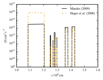
Figure 1: Comparison of prescriptions for the dynamical shear diffusion coefficients. The underlying stellar model is the 20 $M_{\odot}$ star described in Section 3.1. The black, solid line shows the coefficient defined in Eq. 12. The orange, dash-dotted line was computed using Eq. 13.

Brüggen & Hillebrandt (2001) studied the dependence of $D$ on $Ri$ in 3D hydrodynamic simulations of plane-parallel flows. As already mentioned in Section 1, their use of the Boussinesq approximation for the definition of $\mathit{Ri}$ makes it impossible to reconstruct the dependence on the full definition of $\mathit{Ri}$ from the given data.

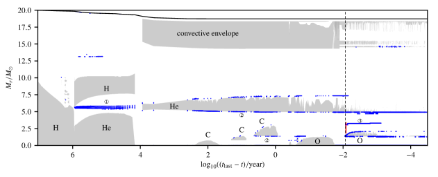
Figure 2: Structure evolution diagram of the $20\,\text{M}_{\odot}$ star with $Z=0.002$ and an initial rotation rate $40\%$ of critical velocity ($\upsilon_{\rm ini}/\upsilon_{\rm crit}=0.4$). The ordinate represents the enclosed mass and the abscissa the time left until the last model, which is in-between core oxygen burning and core silicon burning. The gray zones indicate convective zones. The blue dots mark shells which are unstable to dynamical shear. They can either mark a single unstable zone or an extended region, which is bounded by shear stable layers. The circled numbers refer to different situations in which dynamical shear occurs in stellar models as given in the list in Section 3.2. The core and shell burning regions are indicated with the corresponding element symbol. The vertical dashed line indicates the time that was used as the initial condition for the 2D hydrodynamic simulation. The red area marks the spatial and temporal extent of the 2D simulation.

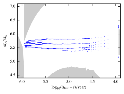
Figure 3: Same as Figure 2 but zoomed in on unstable region at the edge of what was the hydrogen-burning convective core before the beginning of helium burning. The blue dots indicate zones which are unstable to dynamical shear. Each dot indicates an extended shear unstable zone, which is surrounded by shear stable layers. The gray areas are convective regions.

Figure 2 shows the structure evolution diagram for the 20 $M_{\odot}$ model, where convective zones are shaded in gray. The blue dots indicate shells which are unstable to dynamical shear. These can be single zones or extended regions bounded by shear stable layers. This figure thus shows three main types of zones that are unstable to dynamical shear.

The first type appears in the radiative layers from the end of the main sequence onwards. The unstable zones are the result of the combined general core contraction and envelope expansion at the end of core hydrogen burning. One major unstable region appears around the mass coordinate $M_{r}\approx 6\,M_{\odot}$, which corresponds to the edge of the former hydrogen-burning convective core. It is caused by core contraction. It is marked by \raisebox{-0.8pt}{\texttt{1}}⃝ in Fig. 2. A zoom in on this purely radiative, shear unstable region is shown in Fig. 3. At the same evolutionary stage envelope expansion causes another small unstable region between the hydrogen-burning convective shell and the envelope of the star.

The second type is present at convective zone boundaries, where convection redistributes angular momentum very efficiently. This creates a sharp angular velocity gradient at convective zone boundaries, which lowers $\mathit{Ri}$ and is therefore responsible for development of dynamical shear. Examples are marked by \raisebox{-0.8pt}{\texttt{2}}⃝ in Fig. 2.

The third type occurs at the interface of carbon- and neon-rich shells after core oxygen burning. Following the end of core oxygen burning, most of the star undergoes a contraction until the oxygen-burning convective shell develops. This contraction increases the angular velocity gradients and thereby causes the top of the last convective carbon-burning shell to become unstable to shear. It is indicated by \raisebox{-0.8pt}{\texttt{3}}⃝ in Fig. 2.

In this first study of dynamical shear in massive stars, we decided to focus on the last point, unstable zone during the advanced phases, for the following reasons. The evolutionary time scale after core oxygen burning allowed us to cover a significant part of the 1D stellar evolution model in 2D hydrodynamics. In particular we could directly compare the behavior of the instability in both dimensionalities. The smaller length scales of the carbon and neon shells made the computation easier than, for example, the helium shell.

3.3 The Seven-League Hydro code

The numerical tool for the hydrodynamic simulation of the dynamical shear instabilities was the Seven-League Hydro (SLH) code. SLH solves the compressible Euler equations with a finite-volume scheme in one, two, or three spatial dimensions. It offers a range of numerical flux functions, which are specifically tuned to yield accurate results in all Mach number regimes. The calculations presented in this article are computed with the Roe–Miczek method (Miczek et al. 2015). SLH offers the choice of implicit or explicit time stepping for the solution of the hydrodynamics equations. Implicit time stepping is more efficient in the low Mach number regime ($M\lesssim 10^{-2}$). As the maximum Mach number in the inertial frame is 0.5, we choose explicit time integration for the simulation presented in this paper. This cannot be fixed by using a rotating frame of reference because the spread in Mach number between the inner- and outermost layers amounts to 0.1. The explicit time stepping method of choice in SLH is RK3 (Shu & Osher 1988), which is second-order accurate and has excellent stability properties.

A number of different grid geometries are implemented in SLH with the mapped-grid formalism (e.g., Calhoun et al. 2008; Kifonidis & Müller 2012). This allows us to use an arbitrary, structured, curvilinear grid, which is adapted to the problem geometry, but performing all the computations on a logically rectangular grid. The connection between this computational grid and the curvilinear grid is established through a mapping function. Its derivatives enter the finite-volume discretization at several places. In the present case we employed this quite general formalism to create a two-dimensional polar grid as it is best adapted to the geometry of the rotating problem.

The equation of state of choice in this context was the Helmholtz equation of state (Timmes & Swesty 2000), which includes the contributions of radiation, an ideal gas of the nuclei and a Fermi gas of electrons at arbitrary degeneracy. We did not switch on Coulomb corrections. This choice was due to the fact that the equation of state in GENEC – on which our initial conditions are based – does not include them. In the considered range of the star their contribution to pressure and energy is less than 1%. The treatment of electrons in the partially degenerate regime is significantly different in the two codes. To retain the same regions of convective stability in stellar evolution and hydrodynamics we needed to employ a special mapping procedure detailed in Section 4.

4 Model setup

Mapping a one-dimensional stellar evolution model to a multidimensional hydrodynamics code can introduce subtle problems, even if it does not involve rotation. The challenge is to keep the model in hydrostatic equilibrium and preserve many of the thermodynamic properties well, while interpolating on an often much finer grid and possibly applying some smoothing on the very steep gradients introduced by the prescription for convection in the stellar evolution model. Another source of error is the fact that the stellar evolution code might use a different equation of state than the hydrodynamics code.

The condition of hydrostatic equilibrium for a cylindrically symmetric, rotating star is (e.g., Maeder 2009)

$$\frac{\partial P}{\partial r}-\varrho\left(g+r\sin^{2}\vartheta\Omega^{2}\right) =0,$$ (14)

$$\frac{\partial P}{\partial\vartheta}-r\sin\vartheta\cos\vartheta\Omega^{2}\varrho =0.$$ (15)

This assumes the Roche model, meaning that gravity is supposed to be the same as if the mass enclosed in the isobaric shell were located at the center of the star. This implies that the gravitational acceleration is always directed to the center of the star.

A natural choice for performing 2D simulations of a rotating star is the equatorial plane. This is why the following considerations are done in the equatorial plane (colatitude $\vartheta=\pi/2$) of the star only. The $\vartheta$ derivative in Eq. 15 vanishes in this case. To compute the radial pressure profile we can rewrite Eq. 14 as an ordinary differential equation (ODE) for pressure with radius $r$ as the independent variable. We note that, in contrast to Eq. 6, $g(r)$ carries a sign, as the vector $\@vec{g}$ points in negative $r$-direction. This leads to

$$P^{\prime}(r)=\left(g(r)+r\Omega(r)^{2}\right)\varrho(r)\equiv g_{\text{eff}}(r)\varrho(r).$$ (16)

In this form $\varrho(r)$ is just the (interpolated) density profile of the stellar model. An alternate way of computing $\varrho$ is to take the temperature profile of the model and use the equation of state to get $\varrho(T(r),P(r))$. This is needed for reproducing temperature accurately. The same could be done for entropy by using $s(r)$ and computing $\varrho$ as a function of $s(r)$ and $P(r)$ from the equation of state. Here, $P(r)$ is not the value taken from the stellar model but the dependent function in the differential equation. What makes a good choice for the density profile depends on what needs to be reproduced accurately for the problem.

In the case of the current model the most pressing concern was the difference in the equation of state. SLH uses the Helmholtz equation of state while GENEC employs a simpler approximation to a partially degenerate electron gas (see Section 3.3). While the relative difference in pressure is less than $10^{-3}$ (Kippenhahn & Thomas 1964), there is a significant discrepancy in the value of $\nabla_{\text{ad}}$, as shown in Fig. 4. It is clear from the definition of the Brunt–Väisälä frequency that reducing $\nabla_{\text{ad}}$ even by a small amount can cause marginally stable regions in the star to become convectively unstable. As the model was specifically chosen to be convectively stable, this effect is problematic. This is why we used input quantities that differ from the typical choice of density or temperature. Using entropy was not easily possible as it is not readily available from the stellar evolution code. Instead the new model was constructed to reproduce the quantity $\nabla-\nabla_{\text{ad}}$, which determines convective stability, exactly. To this end we needed to extend the ODE Eq. 16 to a system for pressure $P$ and temperature $T$. Here, Density $\varrho(P,T)$ is computed as a function of these two quantities. An expression for $T$ can be derived from Eq. 9,

$$\nabla=\frac{\text{d}\ln T}{\text{d}\ln P}=\frac{P}{T}\frac{\text{d}T}{\text{d}P}=\frac{P}{T}\frac{\text{d}T}{\text{d}r}\frac{\text{d}r}{\text{d}P}=\frac{P}{T\varrho g_{\text{eff}}}\frac{\text{d}T}{\text{d}r}.$$ (17)

To keep $\nabla-\nabla_{\text{ad}}$ identical in the stellar evolution model and the initial setup of the 2D hydrodynamic simulation, we did not use $\nabla(r)$ as an input quantity directly but instead we defined

$$\nabla=\left(\nabla-\nabla_{\text{ad}}\right)_{\text{model}}+\nabla_{\text{ad}}(P,T),$$ (18)

where the expression in the parentheses with subscript “model” was taken from the stellar evolution model and $\nabla_{\text{ad}}(P,T)$ was given by the Helmholtz equation of state, employed in the hydrodynamics code. This leads to a new coupled system of ODEs,

$$P^{\prime}(r) =g_{\text{eff}}(r)\varrho(P,T),$$ (19)

$$T^{\prime}(r) =\frac{T\varrho(P,T)g_{\text{eff}}(r)}{P}\left[\left(\nabla-\nabla_{\text{ad}}\right)_{\text{model}}+\nabla_{\text{ad}}(P,T)\right].$$

The solution of this system matches the convective regions of the stellar evolution code by construction as illustrated in Fig. 5. This even works in the case of a different equation of state. A drawback of this approach is that all other thermodynamic quantities are not guaranteed to reproduce the original model. Fortunately, the deviation is minor for the case at hand as seen in Fig. 6. The condition for the development of a dynamical shear instability is not changed by this mapping procedure as $\Omega$ and $N^{2}$ are identical to the original stellar model.

This approach does not ensure gravity to be consistent with the density field. This could easily be fixed by extending Eq. 19 with an additional equation for the enclosed mass $m$. We did not follow this approach here because the simulation is carried out with a fixed, external gravity field anyway.

The values for the radius that are given in the GENEC simulation are averages over isobaric shells. They correspond to the value at $\vartheta=\arccos\sqrt{1/3}\approx 54.7^{\circ}$, the root of the Legendre polynomial $P_{2}(\cos\vartheta)$. The shape of the isobar $r(\vartheta)$ can be computed from the profiles of $\Omega$. We used the computed value of the equatorial radius and imposed the average $\nabla-\nabla_{\text{ad}}$ on the isobar there. While this is clearly not an exact reconstruction of shellular rotation, as $\nabla-\nabla_{\text{ad}}$ is not constant on isobars, it yields a 2D model that is qualitatively similar to the 1D code, meaning that it has the same convective zones and $\Omega$ profile. The relative change in $T$ and $\varrho$ is less than 8%. An exact reconstruction of the original profile that also preserves convective regions is not possible in this case due to the differences in the equation of state.

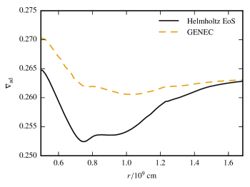
Figure 4: $\nabla_{\text{ad}}$ computed from the equation of state as it is used in GENEC (dashed line) and the value obtained from the Helmholtz equation of state using the same values for density, temperature, and composition as input.

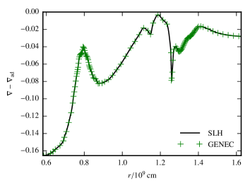
Figure 5: Comparison of the quantity $\nabla-\nabla_{\text{ad}}$ from the GENEC model with the reconstructed values for the Helmholtz equation of state using Eq. 19. This ensures that radiative regions stay radiative after mapping the original data to SLH.

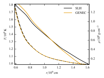
Figure 6: Radial profiles of temperature (solid lines) and density (dashed lines). The yellow lines are the original data from GENEC and the black lines are the initial data for the simulation with SLH, which are reconstructed using the method described in Section 4.

For the radial boundary we used an impenetrable wall boundary on the inner side. This type of boundary condition does not employ ghost cells but directly sets the flux at the interface. The details can be found in Ghidaglia & Pascal (2005). At the outer boundary we left the ghost cells at their initial value. This allows in- and outflow according to the internal flow, while preventing runaway effects caused by extrapolation of the adjacent velocities. There was no boundary in azimuthal direction as we cover the full $2\pi$ azimuthal angle ($\phi$) of the equatorial plane and the geometry is intrinsically periodic. The grid resolution was $512(r)\times 1024(\phi)$ with equidistant spacing. As a convergence test we computed a higher resolution run with $758(r)\times 1536(\phi)$ grid cells and a lower resolution run with $256(r)\times 512(\phi)$. The final angular momentum profile after mixing has stopped is shown in Fig. 7. It demonstrates that the instability starts in all three cases but convergence is only reached with at least 512 radial zones. A study of the second-order structure function of kinetic energy at $t=50\,\text{min}$ showed that the characteristic length scale of the grids with 512 and 758 zones is $1\times 10^{8}\,\text{cm}$, while it is $3\times 10^{8}\,\text{cm}$ in the case of 256 zones. The analysis in this study was done for the simulation with 512 radial zones. At this resolution the average hydrodynamic time step is 1.3 ms. For comparison, the typical GENEC time step at this stage of evolution is about 5 s.

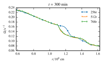
Figure 7: Angular average of angular velocity at $t=300\,\text{min}$ after the shear mixing has stopped. The lines show the profile for simulations with 256, 512, and 768 radial zones. Each have the corresponding number of angular zones to keep the aspect ratio constant.

We did not include any source terms except gravity. Both nuclear reactions and plasma neutrino losses have an influence on the evolution of the instability as well. This is, for example, through the mixing of unburned carbon into the hotter regions below and the resulting increased energy release. The minimum time scale of plasma neutrino losses on the simulation domain, given by the ratio of the total energy to the loss rate, is roughly 300 h. It was estimated using the fitting formulae of Itoh et al. (1996). Nuclear burning acts on the same time scale, although in a different region of the domain. The energy release rate was calculated using one-zone calculations with the nuclear network YANN (Pakmor et al. 2012). Comparing this to the duration of the simulation of $\sim$6 h suggests that both effects are relevant in the dynamic evolution. In our present study, however, we focused purely on the hydrodynamic effects. This was done intentionally to disentangle the effect of the source terms and the hydrodynamic development of the instability, even tough it impedes the possibility to compare the hydrodynamic simulation and the stellar evolution model directly because the latter includes the aforementioned source terms.

5 2D hydrodynamic simulation of dynamical shear

Our goal was to study the development of dynamical shear instabilities in a realistic stellar environment. This was achieved by transferring a model from the stellar evolution code GENEC to the hydrodynamic code SLH. To get an overview of the temporal evolution of the shear instability it is useful to visualize the evolution of the Richardson number, Eq. 4, in different parts of the simulation domain. We computed the Richardson numbers locally on the 2D data and averaged it then on each radius instead of obtaining a 1D profile of the other quantities and calculating $\mathit{Ri}$ from that. This ordering of the averaging operation makes regions containing instabilities more obvious as radial bins containing only few unstable zones are dominated by the often strongly negative values of $\mathit{Ri}$ there. Figure 8 shows the temporal evolution of angular averages of $\mathit{Ri}$. This highlights the region between $1.3\times 10^{9}$ and $1.4\times 10^{9}$ cm, in which we expect the initial development of the shear instability from the well-known theory outlined in Section 2. All figures show the simulation with a radial resolution of 512 grid cells.

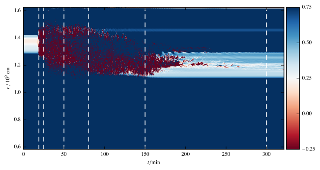
Figure 8: Time evolution of the averaged Richardson number. Blue regions are expected to be stable to dynamical shear. Red regions are Richardson unstable. The Richardson number was computed locally on the 2D data and averaged afterwards. The vertical dashed lines correspond to the 2D snapshots shown in Figs. 10 and 11.

The first obvious result is that the instability developed at the position predicted by the Richardson criterion (indicated by the blue line in the bottom panel of Fig. 9, which is the initial Ri profile in the 2D simulation). We see the growth of the instability to a noticeable level after 19 min of simulation time. The spatial distribution of $\mathit{Ri}$ at this time is depicted in the first panel of Fig. 10. It is still fairly symmetric, dominated by one large-scale mode. This regular pattern is caused by the radially symmetric initial conditions. It shows the typical rolled-up vortex sheets of a Kelvin–Helmholtz instability.

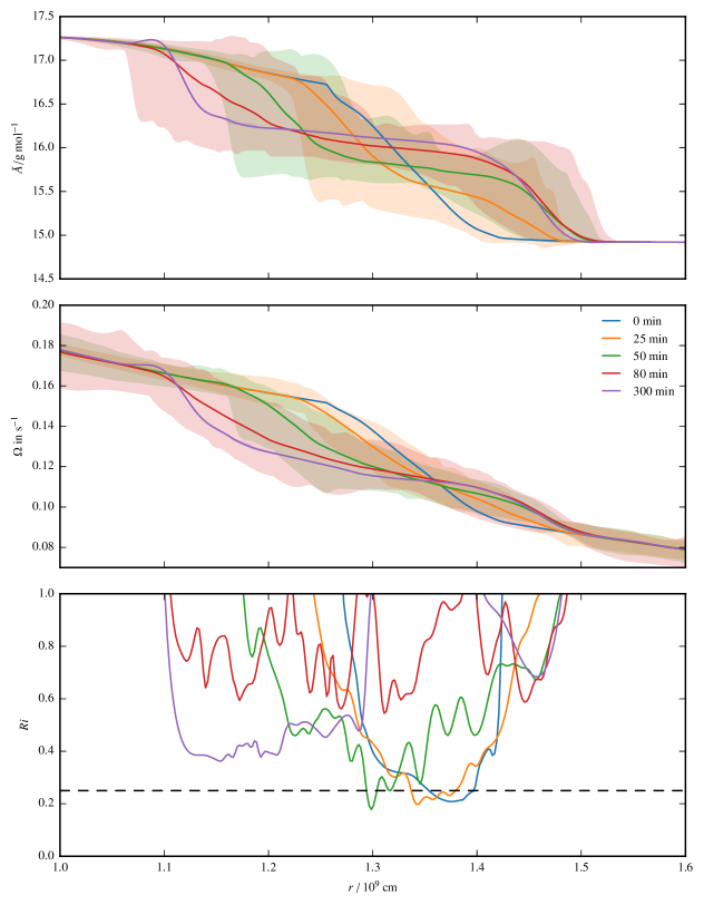
Figure 9: Angular average of mean atomic mass $\bar{A}$, angular velocity $\Omega$, and Richardson number $\mathit{Ri}$ for snapshots at different times indicated by line color. The regions shaded in the respective line color show the range between the minimum and maximum value at the respective radius.

The next panel in Figs. 10 and 11 shows the departure from this very regular pattern at $t=25\,\text{min}$. In the following panels at $t=50\,\text{min}$ and $t=80\,\text{min}$ the flow develops a chaotic structure. This creates a mixed region surrounded by stable layers with the original stratification on top and bottom. The result is a smooth step profile in $\bar{A}$ and angular velocity $\Omega$. The lower edge of this step is the position at which new, smaller shear instabilities develop, causing a further change in the $\Omega$ profile. One case of this is seen at $t=150\,\text{min}$. As a consequence the region affected by the instability expands to lower radii as could already be seen in Fig. 8.

Figure 8 indicates that the unstable regions become smaller after $t=150\,\text{min}$ and have completely disappeared by $t=300\,\text{min}$. Shear mixing has brought $\Omega$ back into the $\mathit{Ri}$-stable regime. The $\bar{A}$ and $\Omega$ profiles go back to a almost perfect cylindrical symmetry. This is illustrated in the first two panels of Fig. 9, where the angular means and the minimum and maximum values almost coincide for $t=300\,\text{min}$.

The bottom panel of Fig. 9 shows the development of the radially averaged profile of the Richardson number. We see how the region with $\mathit{Ri}<0.25$ moves from its initial place between 1.35 and $1.4\times 10^{9}\,\text{cm}$ to smaller radii. In the final state at $t=300\,\text{min}$ there is a significant region where $\mathit{Ri}\approx 0.4$. This indicates that $\mathit{Ri}<0.25$ is indeed the right criterion for the development of dynamical shear instabilities in this case.

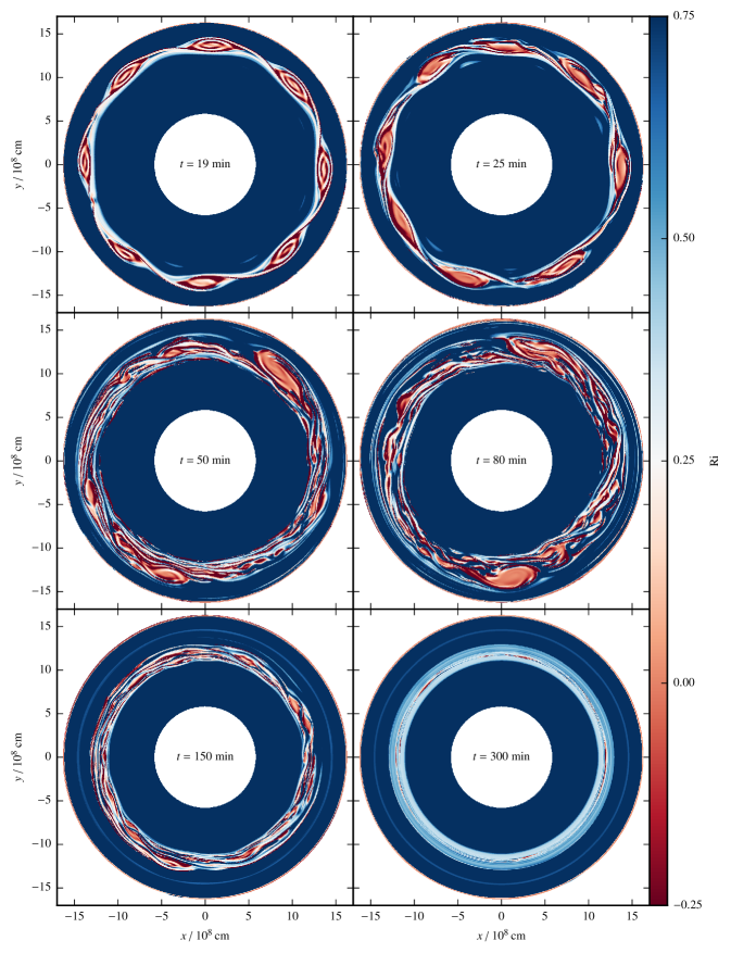
Figure 10: Richardson number in the equatorial plane. The panels correspond to the time steps indicated by vertical lines in Fig. 8. $\mathit{Ri}$ is evaluated along radial profiles. The blue regions are are stable to shear, the red regions are unstable. A movie of the entire simulation is available at https://slh-code.org/papers/dynshear.

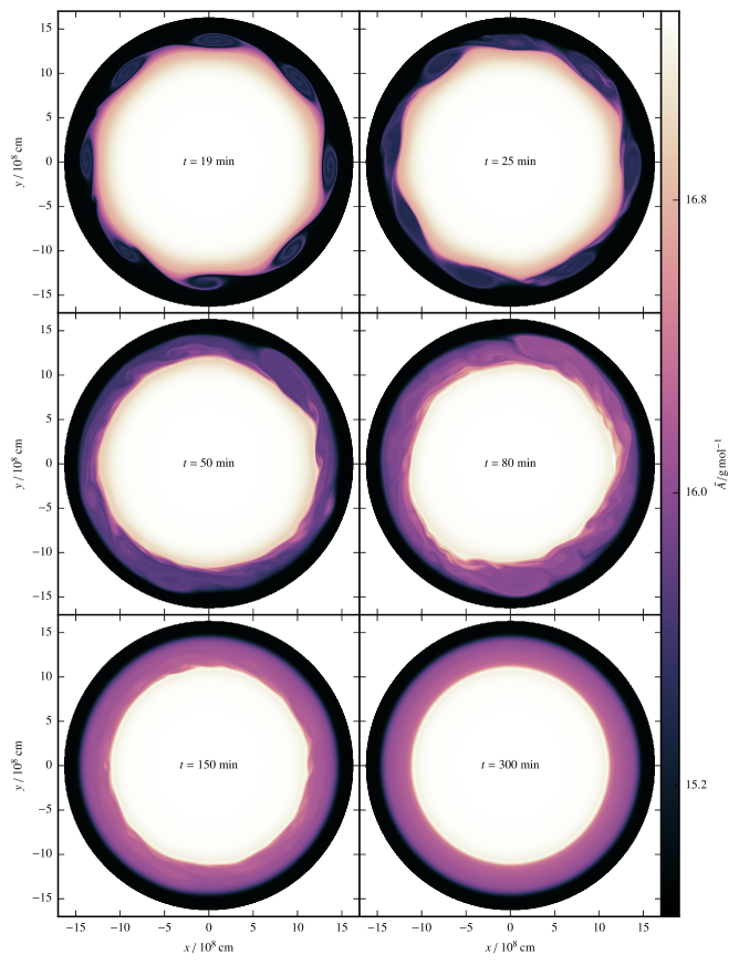
Figure 11: Mean atomic mass $\bar{A}$ in the equatorial plane. The panels correspond to the time steps indicated by vertical lines in Fig. 8.

6 Comparison between 1D and 2D models

The exact time of the onset of the instability in the SLH simulation is marginally later than in the GENEC model as seen in Fig. 12 but this delay has little significance as it mostly depends on the exact time step used for mapping from 1D to 2D. The hydrodynamic simulation starts from a laminar flow so the shear instability needs to grow from an initial perturbation at the level of numerical noise.

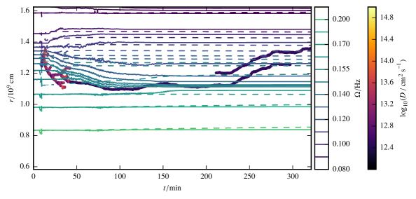
Figure 12: Contour lines of the time evolution of the angular velocity $\Omega$ profile. The solid lines show radial averages of the 2D SLH simulation. The dashed lines show the evolution in the 1D GENEC model with the radial coordinate projected into the equatorial plane. The dots show the location of shear unstable regions in the GENEC simulation. The color of the dots indicate the magnitude of the GENEC diffusion coefficient.

In both the 1D and the 2D model the instability affects the $\Omega$ profile for about 150 min (see Fig. 12), after which it stays virtually constant. The GENEC model still has regions in which dynamical shear is active but with a low value of $D$, so the effect cannot be seen on the timescales considered here. In contrast to the 1D model, the 2D simulation will not change at later times as we do not include any evolutionary processes like nuclear reactions, neutrino losses, contraction, or expansion of the stellar core.

Figure 12 gives an overview of the rearrangement of the angular velocity $\Omega$ profile in both the 1D hydrostatic and 2D hydrodynamic simulation. We see that the instability occurs in both cases shortly after the start of the simulation. Another similarity is that the original instability is quenched by the change in $\Omega$ and new unstable regions are formed in neighboring layers. This is where the details begin to differ. In the 1D case the initial instability evolves much faster. This is due to the fact that a very high diffusion coefficient ($D>10^{13}\,\mathrm{cm}^{2}\,\mathrm{s}^{-1}$) is used in the unstable layer and a very low value in neighboring zones. This moves the strong $\Omega$ gradient to a neighboring cell rather than smoothing it as in the 2D model. After about 50 min the major changes are over and a one-zone, $\mathit{Ri}$ unstable region remains for a time much longer than in the hydro simulation. This does not have a significant impact on the long-term evolution of the $\Omega$ profile as the diffusion coefficient is rather weak in the used prescription. The plot of $\bar{A}$ in Fig. 13 shows that the region affected by shear mixing agrees between 1D and 2D but the magnitude is strongly underestimated by the 1D models. The latter only deviate slightly from the initial condition, whereas the 2D case shows a smooth step profile. If a similar behavior were realized in the GENEC model, this would likely have a noticeable impact on its later evolution. While 3D hydrodynamic simulations are needed to make final quantitative statements, these results indicate that the effect of dynamical shear might be underestimated in its current treatment in stellar evolution codes.

In 1D models mixing due to dynamical shear was implemented by solving a diffusion equation with a temporally and spatially varying diffusion coefficient (see Section 3.2). In the framework of 2D or 3D hydrodynamics such a coefficient is not readily available as the process is not fundamentally of diffusive nature. To ease the comparison the two kinds of simulation it is useful to know what effective diffusion coefficient would be needed to mimic the effect of hydrodynamics, at least on the horizontal averages. We followed the approach of Jones et al. (2017) to compute the diffusion coefficient $D$ necessary to transform the initial profile of $\bar{A}$ to the final profile in one diffusion step. This assumes a constant $D$ over 120 min. The diffusion step is much longer than the time steps of the stellar evolution calculation in this phase and the result is therefore not directly suited for replacing the prescriptions mentioned in Section 3.2. Still, it gave us a measure of the net diffusion caused by the shear instability. The initial and final profiles were obtained by averaging over several hydrodynamics snapshots, corresponding to one GENEC time step.

Some regions can show antidiffusive behavior, that is $D<0$. The diffusion coefficient was set to zero in these cases. To reduce artifacts introduced by starting the computation in a region with a flat profile, we started from both sides and matched the results at the peak of $D$ ($r=1.3\times 10^{9}\,\text{cm}$). The result is shown in Fig. 13. As a benchmark of the quality of the diffusion approximation in this situation we plot $\bar{A}^{\text{rec}}$, the mean atomic mass profile recovered by applying $D$ to the initial profile, as well. It is virtually identical to the final profile $\bar{A}^{\text{fin}}$, which suggests that diffusion is able to reproduce the horizontally averaged profile adequately. To check how strongly $D$ is influenced by the choice of step size we compute diffusion coefficients for a range of smaller step sizes (5 min, 10 min, 20 min). Figure 14 shows these at different times during the simulation. We notice that the step size does not have a strong impact on the diffusion coefficient, at most a factor of about 2.

It is not reasonable to compare this to the shear diffusion coefficient of GENEC at any particular instant because usually only single zones have an extremely large ($D\approx 10^{14}\,\text{cm}^{2}\,\text{s}^{-1}$) value while the coefficient in neighboring zones is zero. This behavior is an artifact of the numerical implementation, in which only unstable zones have a nonzero diffusion coefficient. The form of the diffusion coefficient reconstructed from the hydro simulation underlines the fact that a non-zero diffusion coefficient should be applied to a spatial extent larger than the unstable zones.

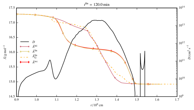
Figure 13: Reconstructed diffusion coefficient from initial and final profiles of mean atomic mass. The initial profile of $\bar{A}^{\text{ini}}$, the final profile of the hydro simulation $\bar{A}^{\text{fin}}$, and the corresponding final profile from GENEC $\bar{A}_{\text{G}}^{\text{fin}}$ are shown. The final state is taken at $t=120\,\text{min}$. The solid black lines shows the effective diffusion coefficient $D$ from the hydro simulation. Negative values due to locally antidiffusive behavior are set to 0. The result of $D$ being applied to the initial $\bar{A}$ profile is shown as $\bar{A}^{\text{rec}}$.

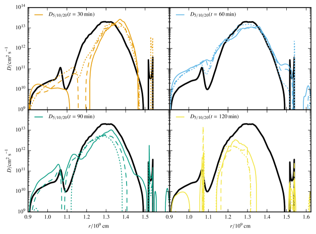
Figure 14: Reconstructed diffusion coefficients calculated at different times during the simulation. The coefficients $D_{5}$ (solid), $D_{10}$ (dashed) and $D_{20}$ (dotted) use a step size of 5 min, 10 min and 20 min, respectively, for the calculation. $D_{120}$ (solid black) is the same as the diffusion coefficient in Fig. 13, i.e. using a step size of 120 min.

7 Conclusions

We performed a 2D hydrodynamic simulation of a dynamical shear instability in a massive star to study their development and the extent of mixing they cause. To start from realistic conditions we use an initial model from the GENEC stellar evolution code. In accordance with linear stability analysis we observe a growing shear instability in regions where $\mathit{Ri}<0.25$. Figure 9 shows that mixing causes the angular velocity profile to become flatter at the center and steeper at the boundaries of the unstable layer. This shifts the unstable region to lower radii until a stable, cylindrically symmetric state is reached. An interesting finding of this work is that these stable regions are in the range $0.25<\mathit{Ri}<1$, despite the fact that the flow here was initially turbulent. This suggests a critical Richardson number of 0.25 for triggering the instability, at least in the considered case, in which no other instabilities are present.

We compare the outcome to the treatment in the 1D stellar evolution code GENEC, which also provided the initial conditions. In addition to the detailed time evolution of the profiles in Figs. 8 and 12, we compute an effective diffusion coefficient from the hydro simulation and compare the initial and final profiles of mean atomic mass to the 1D model. In Figure 13 we observe that the instability occurs in 2D in a qualitatively similar fashion to the 1D hydrostatic prescription. This means the position of the instability, as determined by the Richardson criterion in 1D, is almost the same. A larger quantity of material is mixed in the 2D case. This is not particularly surprising as the value of the diffusion coefficient is not very well constrained by simulations or theory so far (see Section 3.2).

Even very detailed 2D simulations will not give final answers to the nature of the dynamical shear instability. This is due to the differences between 2D and 3D turbulence. An obvious manifestation of this is the long term stability of rolled-up vortex sheets as seen in the first two panels of Fig. 10. A typical observation in the 3D case is that these large-scale structures decay much more quickly to a turbulent state. On a more fundamental level, for 2D turbulence kinetic energy is transported from smaller to larger scales instead of the opposite, which is true for the 3D case. Future work on the hydrodynamics of the dynamical shear instability should therefore ideally use 3D simulations. This is not merely a question of higher computational cost but also raises the issue of how to map a 1D averaged model to an oblate 3D spheroid. Simply adhering to the definition of shellular rotation alone can lead to inconsistent states.

The next step will be to improve the treatment of dynamical shear in 1D codes by considering the results of multidimensional simulations presented in this study. The main point that any 1D implementation of dynamical shear needs to fulfill is that redistribution of angular momentum (and the associated mixing of composition) occurs in regions where $\mathit{Ri}<0.25$ and the instability stops once a stable configuration is reached. Another way of looking at this is that angular momentum will be transported (and mixing will take place) until the angular velocity gradient is shallow enough to be stable everywhere ($\mathit{Ri}>0.25$). Finding the necessary 1D implementation is not an easy task. The current treatment in 1D codes already includes a very efficient transport in unstable layers. The net effect in 1D codes is to shift the steep gradient to the next zone rather than smooth it as in the multidimensional simulations. Using an even higher transport coefficient will not remedy this problem. The different outcome in 1D models is due to the fact that the evolutionary time step is much longer than the timescale of the dynamical shear instability. The higher coefficient found in multidimensional simulations only applies for a small fraction of the evolutionary time step, after which the zones are stable and the coefficient is zero. The improved prescription needs to reproduce the long-term behavior of the instability. Potential avenues to explore are, for example, using an artificially smaller diffusion coefficient in the unstable layer or applying the large diffusion coefficient over a broader region by developing a prescription combining dynamical shear with secular shear (see, e.g., Maeder 1997). These are only suggestions. The details of new prescriptions are beyond the scope of this paper and will be the topic of further studies.