Reconstructing networks of pulse-coupled oscillators from spike trains

Abstract

We present an approach for reconstructing networks of pulse-coupled neuron-like oscillators from passive observation of pulse trains of all nodes. It is assumed that units are described by their phase response curves and that their phases are instantaneously reset by incoming pulses. Using an iterative procedure, we recover the properties of all nodes, namely their phase response curves and natural frequencies, as well as strengths of all directed connections.

I Introduction

Reconstruction of a network structure from observations is an important problem relevant for many different areas such as neuroscience Sporns-05 ; *Riera-05; *Beckmann-05; *Bullmore-Sporns-09; *Rubinov-Sporns-10; *Friston-11; *Chicharro-Andrzejak-Ledberg-11; *Lehnertz-11; *Boly_et_al-12; *Sporns-13, physiology Mrowka_et_al-03 ; *Musizza_et_al-07; *Kralemann_et_al-13, climatology Wang_et_al-12 ; *Sharma_et_al-12, genetics Gardner-04 ; *Zhao-08, ecology Berlow-04 ; *Emmerson-04; *Sugihara26102012; *Gray-15, etc. A group of established reconstruction techniques relies on analysis of the system’s response to a specially designed perturbation, i.e. on invasive measurements Timme-07 ; *Yu-Parlitz-08; *Yu-11; *Levnajic-Pikovsky-11. However, often invasive measurement is not an option, e.g. in problems related to climatology, physiological studies, and medical diagnostics. In such cases one is restricted to analysis of observations of the free-running system.

Roughly speaking, there are two approaches to the problem. The first one does not imply any assumptions about the dynamics of the nodes and properties of the links and relies on different statistical and information-theoretical techniques for quantification of all connections Aertsen-85 ; *Schreiber-00; *Palus-Stefanovska-03; *PhysRevLett.99.204101; *PhysRevLett.100.158101; *PhysRevLett.103.238701; *Chicharro-09; *Andrzejak-11; *PhysRevE.83.051112; *PhysRevLett.108.258701; *Mishchencko-11; *Battaglia-Witt-Wolf-Geisel-12; *Kugiumtzis-13; *Tirabassi-15. In the second, model-based approach, some properties of the nodes (e.g. existence of a stable limit cycle) and of the links (e.g. weakness of coupling) are assumed to be known Rosenblum-Pikovsky-01 ; *Rosenblum_et_al-02; *Kralemann_et_al-07; *Kralemann_et_al-08; Galan-Ermentrout-Urban-05 ; Kralemann-Pikovsky-Rosenblum-11 ; Stevenson-08 ; *Valdes-Sosa-11. In the present work we follow and extend the model-based approach. The main assumption is that the networks can be modeled by coupled limit cycle oscillators Pikovsky-Rosenblum-Kurths-01 ; Izhikevich-07 . In this way we follow our previous studies, where we have reconstructed the connectivity of a weakly coupled network of noisy limit-cycle or weakly chaotic oscillators for the case when the measurements allow for the determination of instantaneous phases Kralemann-Pikovsky-Rosenblum-11 ; Kralemann-Pikovsky-Rosenblum-14 , see also Penny-Litvak-Fuentemilla-Duzel-Friston-09 ; *Cadieu2010; PhysRevLett.109.024101 ; *Rings-Lehnertz-16.

In this paper we address the case when the signals are spiky, namely, that the measurements between the spiking events are dominated by noise and only determination of the times of spikes is reliable. Hence, the data we analyze are spike trains and estimation of time-continuous phase is not feasible. Next, we assume that effect of a chosen unit on the rest of the network is restricted to the time instant when the unit generates a spike. Thus, we use the model of pulse-coupled neuron-like oscillators Mirollo-Strogatz-90 ; *Ernst-Pawelzik-Geisel-95; *vanVreeswijk-96; *Gerstner-96; *Mohanty-Politi-06; *Makarov-05; Memmesheimer-Timme-06 ; *Kinzel-08; *Patnaik-08; *VanBussel-11; *Barranca-16. Assuming that the outputs of all nodes are known and that the coupling between the elements is sufficiently weak to justify the phase dynamics description, we recover the connectivity of the network and properties of all its nodes.

The paper is organized as follows. In Section II we describe in details the model and summarize all the assumptions. In Section III we introduce our technique and in Section IV we present the results of numerical studies. Section V presents discussion of the results.

II The model

Our basic model for the network’s node is a limit cycle oscillator which issues a spike when its phase $\varphi$ achieves $2\pi$. (We consider the phases wrapped to the $[0,2\pi)$ interval, i.e. after the spike generation the phase of the unit is reset to zero). This spike affects all other units of the network according to the strength of the corresponding out-coming connections. Let the size of the network be $N$ and let the connectivity be described by an $N\times N$ coupling matrix ${\cal E}$, whose elements $\varepsilon_{ij}$ quantify the strength of the coupling from unit $j$ to unit $i$. Between the spiking events, phases of all units obey $\dot{\varphi}_{i}=\omega_{i}$, where $\omega_{i}$ are frequencies. If unit $i$ receives a spike from oscillator $j$, then it reacts to the stimulus according to its so-called phase response curve (PRC), $Z_{i}(\varphi)$ Winfree-80 ; *Glass-Mackey-88; Canavier-06 . This means that the phase of the stimulated unit is instantaneously reset, $\varphi_{i}\to\varphi_{i}+\varepsilon_{ij}Z_{i}(\varphi_{i})$.

Notice that oscillators are generally non-identical: they have different frequencies and different PRCs. However, we assume that response of the unit $i$ to the stimuli from different units is described by the same PRC $Z_{i}$. Furthermore, we assume that PRCs are continuous. Next, the coupling is taken to be bidirectional but generally asymmetric, i.e. $\varepsilon_{ji}\neq\varepsilon_{ij}$, and there is no self-action, i.e. $\varepsilon_{ii}=0$.

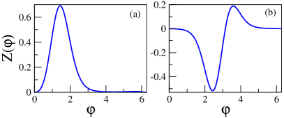
In neuronal modeling one commonly identifies two types of PRCs: if spikes always shorten the period of the stimulated unit, then the PRC is classified as type I. Otherwise, if depending on the phase of the stimulation, the period can be either shortened or prolonged, then the PRC is classified as type II Hansel-Mato-Meunier-95 ; Canavier-06 . We model the type I PRC as

$$Z(\varphi)=(1-\cos(\varphi))\exp{\left(3[\cos(\varphi-\varphi_{0})-1]\right)}\;,$$ (1)

and the type II PRC as

$$Z(\varphi)=-\sin(\varphi)\exp{\left(3[\cos(\varphi-\varphi_{0})-1]\right)}\;,$$ (2)

where the parameter values are $\varphi_{0}=\pi/3$ and $\varphi_{0}=0.9\pi$, respectively. The plots of these curves are shown in Fig. 1.

Figure 1: Model phase response curves of type I (a) and type II (b).

Using this model we generate $N$ point processes (spike trains) and then use them for network reconstruction, where we estimate the coupling matrix ${\cal E}$, PRCs $Z_{i}(\varphi)$, and frequencies $\omega_{i}$ of all elements, as discussed in the next section.

III The technique

For each node we reconstruct its properties as well as strength of all incoming connections. For definiteness, we always determine these quantities for the first node; the procedure then shall be repeated for all other units. Thus, we recover $\varepsilon_{1j}$, $Z_{1}$, and $\omega_{1}$; for simplicity of presentation, in the following we omit the subscript $1$.

We solve the reconstruction problem by iterations. First, since we do not have any a priori knowledge of the system, we assign some values to the coupling coefficients (we discuss several option of how this can be done) and use them in order to obtain a first estimate of the PRC. The knowledge of the latter allows for an improved estimation of the network connectivity, which is then in turn used to obtain a better approximation of the PRC, and so on. We demonstrate that the procedure converges quite fast.

III.1 Notations and phase equations

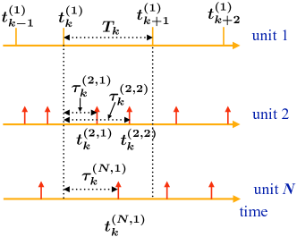
Let the pulse train of the first oscillator contain $M+1$ spikes at times $t_{k}^{(1)}$, so that we have $M$ inter-spike intervals $T_{k}=t_{k+1}^{(1)}-t_{k}^{(1)}$. In the following we treat each interval separately. Suppose that within the inter-spike interval $T_{k}$ the first unit receives $n$ stimuli from the unit $i$, we denote this number as $n_{k}(i)$. These stimuli appear at instants of time $t_{k}^{(i,l)}$, $l=1,\ldots,n_{k}(i)$. The times relative to the beginning of the interval are denoted as $\tau_{k}^{(i,l)}=t_{k}^{(i,l)}-t_{k}^{(1)}$; see Fig. 2 for illustration.

Figure 2: Illustration of notations used. $T_{k}$ is an inter-spike interval of the driven unit. $\tau_{k}^{(i,l)}$ is the time (relative to the beginning of the interval $T_{k}$) when the spike number $l$ from the unit number $i$ arrives.

Respective phases of the first unit are denoted as $\varphi(t_{k}^{(1)}+\tau_{k}^{(i,l)})=\varphi_{k}^{(i,l)}$.

The phase increase within each inter-spike interval is

$$\omega T_{k}+\sum_{i=2}^{N}\varepsilon_{i}\sum_{l=1}^{n_{k}(i)}Z(\varphi_{k}^{(i,l)})=2\pi\;,$$ (3)

where the first term reflects the autonomous dynamics, whereas the second term describes the effect of pulse coupling. $M$ inter-spike intervals yield a system of $M$ Eqs. (3) for unknown coupling coefficients $\varepsilon_{i}$, frequency $\omega$, and the PRC $Z$ of the driven unit.

Assume for the moment that the coupling coefficients $\varepsilon_{i}$ are given. Then, representing the unknown $Z(\varphi)$ as a finite Fourier series of order $N_{F}$, we obtain from Eqs. (3) a system of linear equations for $2N_{F}+1$ Fourier coefficients and the unknown frequency $\omega$. For a long time series, $M>2N_{F}+2$, this is an over-determined system which can be solved, e.g. by a least-mean-square fit or by singular value decomposition, see Pikovsky-16 . On the other hand, if PRC is given, we again obtain a solvable linear system for $N-1$ coupling coefficients $\varepsilon_{i}$ and frequency $\omega$ . Thus, having an initial estimate for either PRC or coupling coefficients (practically we use the later option) we can try to solve Eqs. (3) by iterations.

III.2 First iteration

The phases within each inter-spike interval vary from zero to $2\pi$. For the first iteration we take the simplest approximation, i.e. we compute the phases as growing proportionally to time. Thus, when a spike at $\tau_{k}^{(i,l)}$ arrives, the phase of the first unit is taken as

$$\varphi_{k}^{(i,l)}\approx 2\pi\tau_{k}^{(i,l)}/T_{k}\;.$$ (4)

Since in this approximation we neglect the phase resets, $\varphi\to\varphi+\varepsilon_{i}Z(\varphi)$, the errors of such a phase estimation are of the order of $\varepsilon_{i}\|Z\|$, where $\|\cdot\|$ means norm of the function, and accumulate with the number of the incoming spikes.

Next, we have to choose some initial values for the coupling coefficients $\varepsilon_{i}$. There are several options how to do this. First, we can exploit the simple idea that if there is no connection to the first unit from the unit $i$, then $T_{k}$ cannot depend on the phase when the spikes from this unit appear, i.e. there shall be no dependence of $T_{k}$ on $\varphi_{k}^{(i,1)}$. On the other hand, if this connection exists, the dependence $T_{k}$ on $\varphi_{k}^{(i,1)}$ shall be present as well; moreover, the larger $\varepsilon_{i}$, the stronger this dependence shall be. As shown in Appendix A, this idea indeed works well for long time series. Two further variants are to assign initially same value to all $\varepsilon_{i}$ or take them randomly.

III.3 Next iterations

In the first approximation we compute the phases proportionally to time, see Eq. (4). If the coupling strength, $\varepsilon_{i}$, and parameters of the system, i.e. $\omega$ and $Z$, are already estimated, then we can use this knowledge for a more precise estimation of the phases. For illustration, suppose that within the inter-spike interval $T_{k}$ the first unit receives three stimuli at times $\tau_{k}^{(i,1)}<\tau_{k}^{(m,1)}<\tau_{k}^{(n,1)}$. Then the phases at these three instances are computed as

$$\varphi_{k}^{(i,1)} =\omega\tau_{k}^{(i,1)}\;,$$

$$\varphi_{k}^{(m,1)} =\omega\tau_{k}^{(m,1)}+\varepsilon_{i}Z\left(\varphi_{k}^{(i,1)}\right)\;,$$

$$\varphi_{k}^{(n,1)} =\omega\tau_{k}^{(n,1)}+\varepsilon_{i}Z\left(\varphi_{k}^{(i,1)}\right)+\varepsilon_{m}Z\left(\varphi_{k}^{(m,1)}\right)\;.$$

The phase at the end of the given inter-spike interval is

$$\psi=\omega T_{k}+\varepsilon_{i}Z(\varphi_{k}^{(i,1)})+\varepsilon_{m}Z\left(\varphi_{k}^{(m,1)}\right)+\varepsilon_{n}Z\left(\varphi_{k}^{(n,1)}\right)\;.$$

By definition, this value should be equal to $2\pi$. However, since $\omega$ and $Z$ are not exact, $\psi$ generally differs from $2\pi$. Therefore, we re-scale all phase estimates by the factor $2\pi/\psi$.

Now, using the newly estimated phases and the estimation of the PRC from the previous iteration, we can compute new values of the coupling coefficients $\varepsilon_{i}$, and then repeat the whole procedure. As we demonstrate below, these iterations converge quite quickly.

IV Numerical tests

In this section we present the results of numerical testing of our reconstruction algorithm. For this goal we generate the networks with some randomly chosen parameters and then compare the reconstructed values with the true ones. Namely, we consider networks of $N=20$ oscillators, with natural frequencies taken from a uniform distribution between 1 and 2. Strength of network links is sampled from the positive half of a Gaussian distribution with zero mean and standard deviation $0.02$. We excluded from the consideration the networks where at least two units synchronized. The frequency of the first oscillator is set to 1, assuring that it is the slowest one (as discussed below, this is the most difficult case) and then we reconstruct its PRC $Z$, frequency $\omega$, and strength of all incoming links $\varepsilon_{i}$, $i=2,\ldots,20$. We use ten iterations of the procedure described above.

Before presenting the results we recall that all equations contain only the products of $\varepsilon_{i}$ and $Z$. Hence, solutions $\varepsilon_{i},Z$ and $c\varepsilon_{i},Z/c$, where $c$ is an arbitrary constant, are equivalent. The factor $c$ has no physical meaning by itself, but since we want to compare the reconstructed values with the originally given, we have to fix it. Quite arbitrarily, we do it by minimizing

$$\sum\limits_{i=2}^{N}\left[\varepsilon_{i}^{\text{(t)}}-c\varepsilon_{i}^{\text{(r)}}\right]^{2}$$

where the superscripts (t) and (r) stand for true and reconstructed, respectively. This condition yields

$$c=\sum\limits_{i=2}^{N}\varepsilon_{i}^{\text{(t)}}\varepsilon_{i}^{\text{(r)}}\bigg{/}\sum\limits_{i=2}^{N}\left[\varepsilon_{i}^{\text{(t)}}\right]^{2}\;.$$ (5)

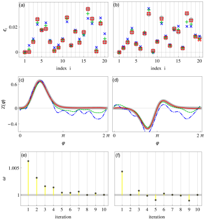
Using this normalization, we show the results of a particular run in Fig. 3; for this computation we took initially $\varepsilon_{i}=1\,,\;\forall i$.

Figure 3: (Color online) Reconstruction of a network of 20 units using $M=200$ inter-spike intervals. Panels (a,c,e) and (b,d,f) show the results for PRC type I and PRC type II, respectively, see Eqs. (1,2). (a,b) Strength of the incoming connections to the first oscillator: true values (gray disks) and values recovered after one, 2, and 10 iterations (blue crosses, green pluses, and red hash-tag, respectively). (c,d) True (wide gray curve) and reconstructed PRCs, after one, 2, and 10 iterations (blue dashed-dotted, green dashed, and red solid curves, respectively). (e,f) Estimated natural frequencies as functions of the iteration number; the true value $\omega=1$ is shown by horizontal gray line.

Next, we perform a statistical analysis for $10^{5}$ network configurations. To quantify the quality of the reconstruction, we define the corresponding errors for recovered PRC, $\varepsilon_{i}$ and $\omega$ as

$$\Delta^{2}_{\text{PRC}}=\frac{\int_{0}^{2\pi}\left[Z^{(\text{t})}(\varphi)-Z^{(\text{r})}(\varphi)\right]^{2}d\varphi}{\int_{0}^{2\pi}\left[Z^{(\text{t})}(\varphi)\right]^{2}d\varphi}\;,$$ (6)

$$\Delta^{2}_{\varepsilon}=\sum_{i=2}^{N}\big{[}\varepsilon_{i}^{(\text{t})}-\varepsilon_{i}^{(\text{r})}\big{]}^{2}\bigg{/}\sum_{i=2}^{N}\big{[}\varepsilon_{i}^{(\text{t})}\big{]}^{2}\;,$$ (7)

and

$$\Delta^{2}_{\omega}=\big{[}\omega^{(\text{t})}-\omega^{(\text{r})}\big{]}^{2}\;.$$ (8)

respectively . The distributions of errors, shown in Fig. 4, confirm robustness of the iterative procedure.

Figure 4: (Color online) Histograms of errors of the coupling strengths $\Delta_{\varepsilon}$ (a,b), PRC $\Delta_{\text{PRC}}$ (c,d), and frequency $\omega$ (e,f), see Eqs. (6-8). Panels (a,c,e) and (b,d,f) correspond to tests with PRC type I and type II, respectively. In each panel the results of the first, third, and tenth iterations are shown in blue (dash-dotted), green (dashed), and red (solid line) respectively. In (a,b) also the distribution of errors for initial values $\varepsilon_{i}=1$ is shown in orange (dotted line).

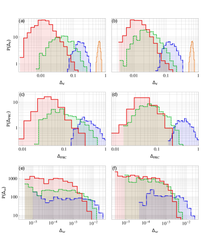
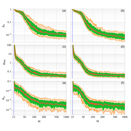
Figure 5 shows the dependence of the reconstruction error on the number of inter-spike intervals. Naturally, the more data we use, the better results we expect. This test demonstrates, that reasonable reconstruction can be achieved already for several hundreds of intervals.

Figure 5: (Color online) Error of the reconstruction in dependence on the number of inter-spike intervals $M$ used for the analysis. Panels (a,c,e) and (b,d,f) show the results for PRC type I and PRC type II, respectively. Panels (a,b) show the error of the coupling coefficients $\varepsilon_{i}$ (6), panels (c,d) the error of the PRC (7) and panels (e,f) the error of the frequency $\omega$ (8). For each value of $M$ reconstruction error was computed for 6000 different networks. The green (dark gray) and the orange (light gray) areas contain 50% and 75% of the errors, respectively; the median is shown in red (bold line).

Finally, we performed the test with random assignment of the initial values for the coupling coefficients $\varepsilon_{i}$. For several generated networks we performed $10^{4}$ reconstructions with different initial $\varepsilon_{i}$. The results confirm convergence of the algorithm for this case as well.

IV.1 Network of Morris-Lecar neurons

In the next test we make a step towards more realistic modeling and consider a network of Morris-Lecar neurons Morris-Lecar-81 ; *Rinzel-Ermentrout-98. The equations of the network are:

$$\begin{split}\dot{V}_{i}=&I_{i}-g_{l}(V_{i}-V_{l})-g_{K}w_{i}(V_{i}-V_{k})\\ &-g_{Ca}m_{\infty}(V_{i})(V_{Ca}-V_{i})+I_{i}^{\text{(syn)}}\;,\\[4.30554pt] \dot{w}_{i}=&\lambda(V_{i})(w_{\infty}(V_{i})-w_{i})\;,\end{split}$$ (9)

where

$$\begin{split}m_{\infty}(V)&=[1+\tanh{(V-V_{1}/V_{2})}]/2\;,\\ w_{\infty}(V)&=[1+\tanh{(V-V_{3}/V_{4})}]/2\;,\\ \lambda(V)&=\cosh{[(V-V_{3})/2V_{4}]}/3\;,\end{split}$$ (10)

and $I_{i}^{\text{(syn)}}$ is the total incoming synaptic current. We write the latter as

$$I_{i}^{\text{(syn)}}=\left[V_{\text{rev}}-V_{i}\right]\sum_{k,k\neq i}\frac{\varepsilon_{ik}}{1+\exp{\left[-(V_{i}-V_{\text{th}})/\sigma\right]}}\;.$$ (11)

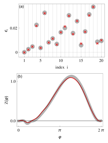
We take standard values for most of the parameters . Parameters of the synaptic coupling are $V_{\text{rev}}=0.2$, $V_{\text{th}}=0.25$, and $\sigma=0.01$. The neurons are non-identical: the values of the current are $I_{i}=0.077(1+0.22\xi)$, where $\xi$ is uniformly distributed between zero and one; for these values the neurons remain in the spiking state. The results of the analysis with $200$ inter-spike intervals shown in Fig. 6, confirm efficiency of our technique.

Figure 6: (Color online) Reconstruction of a network of 20 Morris-Lecar neuronal oscillators, see Eqs. (9-11). 200 inter-spike intervals were used for the reconstruction. (a) True values of the strength of the incoming connections for the first neuron (gray disks) and these values reconstructed after 10 iterations (red crosses). (b) True (wide gray curve) and reconstructed (solid red curve) PRC.

V Discussion and conclusions

With the help of two model systems we have demonstrated, that our technique provides a robust reconstruction of a network. The data requirements are not too demanding: the reconstruction is quite precise already for time series of several hundreds of spikes. Now we discuss some limitations of the method.

First we comment on the initial estimate of phases using Eq. (4). As already mentioned, the error is proportional to $\varepsilon_{i}\|Z\|$ and increases with the number of spikes that arrive within the inter-spike interval of the driven unit. This explains why the case of the slowest oscillator is the most difficult one: such an oscillator has on average more incoming stimuli per inter-spike interval then the fast units. This means, that though our examples demonstrate robust reconstruction, it may fail if $\omega_{i}/\omega_{1}\gg 1$.

Next limitation is related to variability of the inter-spike intervals of the driving unit $i$ (for $\omega_{i}>\omega_{1}$). Indeed, suppose that drive is strictly periodic. Then time of the appearance of the first spike unambiguously determines the timing of the following ones, and hence, the length of the inter-spike interval $T_{k}$. However, $T_{k}$ is then determined by the sum of different pieces of PRC and this sum cannot be disentangled. The initial estimation of the strength of the connection as described in Appendix A can still work, but the recovery of the PRC becomes impossible and the iterative procedure fails. So, we foresee that reconstruction may be not so robust for very sparse network where we expect to have purely periodic nodes. On the other hand, a realistic network is noisy, and noise naturally provides the desired variability in the time series, thus enhancing the reconstruction. Finally, we mention that the reconstruction fails if the network synchronizes.

Appendix A First estimation of incoming connections

For sufficiently long data an initial estimation of the coupling strength $\varepsilon_{i}$ can be performed by evaluating the effect of the first pulse from the unit $i$, that arrives within the $k$-th inter-spike interval, on the length of this interval $T_{k}$. For this purpose, we first plot $T_{k}$ vs $\varphi_{k}^{(i,1)}$, for all incoming links. Next, for each plot, we divide the $\varphi$-axis into $N_{b}$ bins and average the $T_{k}$ values within each bin. As a result, we obtain a dependence $\bar{T}^{(i)}_{n}\left(\bar{\varphi}_{n}\right)$, where $\bar{\varphi}_{n}=\frac{\pi}{N_{b}}(2n-1)$, $n=1,\ldots,N_{b}$, are phases at the centers of bins. Our conjecture is that $\bar{T}^{(i)}_{n}\left(\bar{\varphi}_{n}\right)$ reflects the strength of the incoming connection: if this strength is zero, i.e. there is no incoming link from unit $i$, then there shall be no dependence; on the other hand, if the incoming connection is strong, then we expect the dependence to be well-pronounced.

We illustrate this idea in Fig. 7, where two such plots are shown for the cases of weak and strong incoming connections.

Figure 7: (Color online) Scatter plots of inter-spike intervals $T_{k}$ vs. approximated phase $\varphi_{k}^{(i,1)}$ of the first spike from a chosen driving oscillator $i$, for a strong coupling strength (a) and for a weak one (b). The horizontal axis is divided into $N_{b}=50$ bins and solid red curve shows the average of $T_{k}$ over each of the bins, $\bar{T}^{(i)}$, as a function of the central phase $\bar{\varphi}$ of the bins; $2\cdot 10^{4}$ inter-spike intervals are used in this computation.

We see that indeed $\bar{T}^{(i)}_{n}\left(\bar{\varphi}_{n}\right)$ reflects the coupling coefficients $\varepsilon_{i}$. Hence, we use the standard deviation of this dependence as the first estimate, i.e. we take

$$\varepsilon_{i}=\Big{\langle}\big{(}\bar{T}^{(i)}_{n}-\langle\bar{T}^{(i)}_{n}\rangle\big{)}^{2}\Big{\rangle}^{1/2}\;,$$ (12)

where $\langle\cdot\rangle$ means averaging over $N_{b}$ bins. Although the correspondence between the estimate and true coupling strength is not exact, in most cases this approach yields reasonable values.

References

- (1) O. Sporns, G. Tononi, and R. Kotter, Computational Biology 1(4), 245 (2005)
- (2) J. Riera et al., Phil. Trans. R. Soc. B 360, 1025 (2005)
- (3) C. F. Beckmann et al., Phil. Trans. R. Soc. B 360, 1001 (2005)
- (4) E. Bullmore and O. Sporns, Nature Reviews Neuroscience 10, 187 (2009)
- (5) M. Rubinov and O. Sporns, NeuroImage 52, 1059 (2010)
- (6) K. J. Friston, Brain Connectivity 1, 13 (2011)
- (7) D. Chicharro, R. Andrzejak, and A. Ledberg, BMC Neuroscience 12, P192 (2011), ISSN 1471-2202, http://www.biomedcentral.com/1471-2202/12/S1/P192
- (8) K. Lehnertz, Physiological Measurement 32, 1715 (2011)
- (9) M. Boly, M. Massimini, M. Garrido, O. Gosseries, Q. Noirhomme, S. Laureys, and A. Soddu, Brain Connectivity 2, 1 (2012)
- (10) O. Sporns, Nature Methods 10, 491 (2013)
- (11) R. Mrowka, L. Cimponeriu, A. Patzak, and M. Rosenblum, American J. of Physiology Regul. Comp. Integr. Physiol. 145, R1395 (2003)
- (12) B. Musizza, A. Stefanovska, P. V. E. McClintock, M. Paluš, J. Petrovčič, S. Ribarič, and F. Bajrovič, J Physiol 580, 315 (2007)
- (13) B. Kralemann, M. Frühwirth, A. Pikovsky, M. Rosenblum, T. Kenner, J. Schaefer, and M. Moser, Nature Communications 4, 2418 (2013)
- (14) G. Wang, P. Yang, X. Zhou, K. L. Swanson, and A. A. Tsonis, Geophys. Res. Lett. 39, L13704 (2012)
- (15) S. Das Sharma, D. S. Ramesh, C. Bapanayya, and P. A. Raju, J. Geophys. Res. 117, D13110 (2012)
- (16) T. S. Gardner et al., Science 301, 102 (2003)
- (17) W. Zhaoa, E. Serpedin, and E. R. Dougherty, Transactions on Computational Biology and Bioinformatics 5(2), 262 (2008)
- (18) E. L. Berlow et al., Journal of Animal Ecology 73, 585 (2004)
- (19) M. C. Emmerson and D. Raffaelli, Journal of Animal Ecology 73, 399 (2004)
- (20) G. Sugihara, R. May, H. Ye, C.-h. Hsieh, E. Deyle, M. Fogarty, and S. Munch, Science 338, 496 (2012)
- (21) C. Graya, D. H. Figueroa, L. N. Hudson, A. Ma, D. Perkins, and G. Woodward, Food Webs 5, 11 (2015)
- (22) M. Timme, Physical Review Letters 98, 224101 (2007)
- (23) D. Yu and U. Parlitz, EPL (Europhysics Letters) 81, 48007 (2008), http://stacks.iop.org/0295-5075/81/i=4/a=48007
- (24) D. Yu and U. Parlitz, PLoS ONE 6(9) (2011)
- (25) Z. Levnajić and A. Pikovsky, Phys. Rev. Lett. 107, 034101 (Jul 2011), http://link.aps.org/doi/10.1103/PhysRevLett.107.034101
- (26) A. Aertsen and G. L. Gerstein, Brain Res. 340, 341â354 (1985)
- (27) T. Schreiber, Phys. Rev. Lett. 85, 461 (2000)
- (28) M. Paluŝ and A. Stefanovska, Phys. Rev. E 67, 055201 (2003)
- (29) S. Frenzel and B. Pompe, Phys. Rev. Lett. 99, 204101 (Nov 2007), http://link.aps.org/doi/10.1103/PhysRevLett.99.204101
- (30) M. Staniek and K. Lehnertz, Phys. Rev. Lett. 100, 158101 (Apr 2008), http://link.aps.org/doi/10.1103/PhysRevLett.100.158101
- (31) L. Barnett, A. B. Barrett, and A. K. Seth, Phys. Rev. Lett. 103, 238701 (Dec 2009), http://link.aps.org/doi/10.1103/PhysRevLett.103.238701
- (32) D. Chicharro and R. G. Andrzejak, PRE 80, 026217 (2009)
- (33) R. G. Andrzejak and D. Chicharro and K. Lehnertz and F. Mormann, PRE 83, 046203 (2011)
- (34) L. Faes, G. Nollo, and A. Porta, Phys. Rev. E 83, 051112 (May 2011), http://link.aps.org/doi/10.1103/PhysRevE.83.051112
- (35) J. Runge, J. Heitzig, V. Petoukhov, and J. Kurths, Phys. Rev. Lett. 108, 258701 (Jun 2012), http://link.aps.org/doi/10.1103/PhysRevLett.108.258701
- (36) Y. Mishchencko and J. T. Vogelstein, The Annals of Applied Statistics 5, 1229 (2011)
- (37) D. Battaglia, A. Witt, F. Wolf, and T. Geisel, PLoS computational biology 8, e1002438 (2012)
- (38) D. Kugiumtzis, Phys. Rew. E 87, 062918 (2013)
- (39) G. Tirabassi et al., Scientific Reports 5, 10829 (2015)
- (40) M. G. Rosenblum and A. S. Pikovsky, Phys. Rev. E 64, 045202 (2001)
- (41) M. G. Rosenblum, L. Cimponeriu, A. Bezerianos, A. Patzak, and R. Mrowka, Phys. Rev. E 65, 041909 (2002)
- (42) B. Kralemann, L. Cimponeriu, M. Rosenblum, A. Pikovsky, and R. Mrowka, Phys. Rev. E 76, 055201 (2007)
- (43) B. Kralemann, L. Cimponeriu, M. Rosenblum, A. Pikovsky, and R. Mrowka, Phys. Rev. E 77, 066205 (2008)
- (44) R. F. Galán, G. B. Ermentrout, and N. N. Urban, Phys. Rev. Lett. 94, 158101 (2005)
- (45) B. Kralemann, A. Pikovsky, and M. Rosenblum, Chaos 21, 025104 (2011)
- (46) I. H. Stevenson et al., Current Opinion in Neurobiology 18, 582â588 (2008)
- (47) P. A. Valdes-Sosa et al., NeuroImage 58, 339 (2011)
- (48) A. Pikovsky, M. Rosenblum, and J. Kurths, Synchronization. A Universal Concept in Nonlinear Sciences. (Cambridge University Press, Cambridge, 2001)
- (49) E. M. Izhikevich, Dynamical Systems in Neuroscience (MIT Press, Cambridge, Mass., 2007)
- (50) B. Kralemann, A. Pikovsky, and M. Rosenblum, New Journal of Physics 16, 085013 (2014)
- (51) W. Penny, V. Litvak, L. Fuentemilla, E. Duzel, and K. Friston, Journal of Neuroscience Methods 183, 19 (2009)
- (52) C. Cadieu and K. Koepsell, Neural Computation 22, 3107 (Dec. 2010), ISSN 0899-7667, http://www.mitpressjournals.org/doi/abs/10.1162/NECO_a_00048
- (53) T. Stankovski, A. Duggento, P. V. E. McClintock, and A. Stefanovska, Phys. Rev. Lett. 109, 024101 (Jul 2012)
- (54) T. Rings and K. Lehnertz, Chaos: An Interdisciplinary Journal of Nonlinear Science 26, 093106 (2016), http://dx.doi.org/10.1063/1.4962295, http://dx.doi.org/10.1063/1.4962295
- (55) R. Mirollo and S. Strogatz, SIAM J. Appl. Math. 50, 1645 (1990)
- (56) U. Ernst and K. Pawelzik and T. Geisel, Phys. Rev. Lett. 74, 1570 (1995)
- (57) C. van Vreeswijk, Phys. Rev. E 54, 5522 (1996)
- (58) W. Gerstner, Phys. Rev. Lett. 76, 1755 (1996)
- (59) P. Mohanty and A. Politi, J. Phys. A: Math. Gen. 39, L415 (2006)
- (60) V. A. Makarov, F. Panetsos, and O. de Feo, Journal of Neuroscience Methods 144, 265 (2005)
- (61) R.-M. Memmesheimer and M. Timme, Phys. Rev. Lett. 97, 188101 (2006)
- (62) W. Kinzel, J. Comput. Neurosci. 24, 105 (2008)
- (63) D. Patnaik, P. Sastry, and K. Unnikrishnan, Scientific Programming 16, 49â77 (2008)
- (64) F. V. Bussel, B. Kriener, and M. Timme, Front. Comput. Neurosci. 5 (2011)
- (65) V. J. Barranca, D. Zhou, and D. Cai, PRE 93, 060201 (2016)
- (66) A. T. Winfree, The Geometry of Biological Time (Springer, Berlin, 1980)
- (67) L. Glass and M. C. Mackey, From Clocks to Chaos: The Rhythms of Life. (Princeton Univ. Press, Princeton, NJ, 1988)
- (68) C. C. Canavier, Scholarpedia 1(12), 1332 (2006)
- (69) D. Hansel, G. Mato, and C. Meunier, Neural Comput. 7, 307 (1995)
- (70) A. Pikovsky, Phys. Rev. E 93, 062313 (2016)
- (71) When neither PRC nor are known, Eqs. (3) represent a nonlinear system with respect to unknowns. Alternatively, one could consider products of and the Fourier coefficients as unknowns and end up with a linear, but rather large system of unknowns.
- (72) Notice that error is minimized due to normalization according to Eq. (5).
- (73) C. Morris and H. Lecar, Biophys. J. 35, 193 (1981)
- (74) J. Rinzel and B. Ermentrout, in Methods of Neuronal Modeling, edited by C. Koch and I. Segev (MIT Press, Cambridge, 1998) pp. 251–292
- (75) Parameters of the system (9,10) are: , , , , , , , , , .