Optimal Query Time for Encoding Range Majority

Abstract

We revisit the range $\tau$-majority problem, which asks us to preprocess an array $\mathsf{A}[1..n]$ for a fixed value of $\tau\in(0,1/2]$, such that for any query range $[i,j]$ we can return a position in $\mathsf{A}$ of each distinct $\tau$-majority element. A $\tau$-majority element is one that has relative frequency at least $\tau$ in the range $[i,j]$: i.e., frequency at least $\tau(j-i+1)$. Belazzougui et al. [WADS 2013] presented a data structure that can answer such queries in $\mathcal{O}(1/\tau)$ time, which is optimal, but the space can be as much as $\Theta(n\lg n)$ bits. Recently, Navarro and Thankachan [Algorithmica 2016] showed that this problem could be solved using an $\mathcal{O}(n\lg(1/\tau))$ bit encoding, which is optimal in terms of space, but has suboptimal query time. In this paper, we close this gap and present a data structure that occupies $\mathcal{O}(n\lg(1/\tau))$ bits of space, and has $\mathcal{O}(1/\tau)$ query time. We also show that this space bound is optimal, even for the much weaker query in which we must decide whether the query range contains at least one $\tau$-majority element.

1 Introduction

Misra and Gries [14] generalized a classic $2$-pass algorithm by Boyer and Moore [3] for finding majorities in lists of elements. Formally, a $\tau$-majority of a list of length $n$ (or $\tau$-heavy-hitter) is an element that appears with frequency at least $\tau\cdot n$. More recent variants and improvements [5, 12] to the Misra-Gries algorithm have become standard tools in a wide variety of applications involving streaming analytics, such as IP traffic monitoring, data mining, etc.

In this paper we consider the data structure variant of the problem. Suppose we are given an array $\mathsf{A}$ of $n$ elements. The goal is to preprocess the array into a data structure that supports range $\tau$-majority queries: given an arbitrary subarray $\mathsf{A}[i..j]$, return all distinct elements that are $\tau$-majorities in $\mathsf{A}[i..j]$. As an example application, we may wish to construct such a data structure on network traffic logs, to perform an analysis of how the set of frequent users change over different timescales.

In the last few years, this problem has received a lot of attention [13, 6, 9, 2], finally leading to a recent result of Belazzougui et al. [2, 1]: these queries can be supported in $\mathcal{O}(1/\tau)$ time, using $(1+\varepsilon)nH_{0}+o(n)$ bits of space, where $H_{0}$ is the zero-th order empirical entropy of the array $\mathsf{A}$, and $\varepsilon$ is an arbitrary positive constant. Since, for an arbitrary $\tau$-majority query, there can be $\lfloor 1/\tau\rfloor$ answers, there is not much hope for significantly improving the query time of $\mathcal{O}(1/\tau)$, except perhaps to make the time bound output-sensitive on the number of results returned [1, Sec.7].

On the other hand, much more can be said about the space bound. Note that, in general, if $\mathsf{A}$ contains elements drawn from the alphabet $[1,\sigma]$, then we can represent it using $n\lceil\lg\sigma\rceil$ bits. If $f_{i}$ is the frequency of element $i\in[1,\sigma]$, then we have $nH_{0}=n\sum_{i}\left((f_{i}/n)\lg(n/f_{i})\right)\leq n\lceil\lg\sigma\rceil$. Since the bound of Belazzougui et al. [1] depends on the entropy of the elements in $\mathsf{A}$, it can therefore can be $\Theta(n\lg n)$ bits, if $\sigma=\Omega(n^{c})$ for any constant $c\leq 1$, and the distribution is close to uniform. However, quite recently, Navarro and Thankachan [15] showed that this space bound can be improved significantly in the encoding model.

In the encoding model, given array $\mathsf{A}$ as input, we are allowed to construct an encoding that supports a specific query operation on $\mathsf{A}$. After constructing the encoding, the array $\mathsf{A}$ is deleted, and queries must be supported by accessing only the encoding. For many query operations, we can achieve space bounds that are much smaller than the space required to store $\mathsf{A}$. One issue is that for range $\tau$-majority queries, if we return the actual element which is a $\tau$-majority, then we must store at least as many bits as are required to represent $\mathsf{A}$. This follows since an encoding supporting such queries can be used to return the contents of the array $\mathsf{A}$ by querying the range $\mathsf{A}[i..i]$ for each $1\in[1,n]$.

Navarro and Thankachan [15] therefore considered a different query, in which, for each $\tau$-majority $a$ in the query range $\mathsf{A}[i..j]$, we instead return an arbitrary position $\ell$ in $\mathsf{A}$ such that $\mathsf{A}[\ell]=a$ and $i\leq\ell\leq j$. In the remainder of the paper, we use range $\tau$-majority position query to refer to this positional variant of the query operation. Navarro and Thankachan [15] showed two main results:

Theorem 1.1 ([15], Theorems 1 and 2)

1. For any $\tau\in(0,1)$, there is an encoding that occupies $\mathcal{O}(n\lceil\lg(1/\tau)\rceil)$ bits of space that supports range $\tau$-majority position queries in:

   1. $\mathcal{O}((1/\tau)\lg n)$ time if $1/\tau=o(\textup{polylog}(n))$.

   2. $\mathcal{O}(1/\tau)$ time if $1/\tau=\Theta(\textup{polylog}(n))$.

   3. $\mathcal{O}(1/\tau\lg\lg_{w}(1/\tau))$ time if $1/\tau=\omega(\textup{polylog}(n))$.

2. Any encoding that can support range $\tau$-majority counting queries (i.e., return the total the number of $\tau$-majorities) in an arbitrary query range $\mathsf{A}[i..j]$ occupies space (in bits) at least $\frac{n}{4}\left(\lg\left(\frac{1}{2\tau}-1\right)-\lg e\right)=\Omega(n\lg(1/\tau))$.

Thus, their lower bound implies that their space bound, which depends only on $n$ and $\tau$ rather than elements in the input array $\mathsf{A}$, is optimal. However, there is gap between the query time of their encoding and the data structure of Belazzougui et al. [1] for the case where $1/\tau$ is not $\Theta(\textup{polylog}(n))$. Crucially, this does not yield optimal time in the important case where $1/\tau$ is a constant. In this paper, we close this time gap, and prove the following theorem:

Theorem 1.2

For any $\tau\in(0,1/2]$, there is an encoding that occupies $\mathcal{O}(n\lg(1/\tau))$ bits of space that can answer range $\tau$-majority position queries in $\mathcal{O}(1/\tau)$ time.

Of course one could ask if $\mathcal{O}(1/\tau)$ is the right bound for the query time at all. In the output-sensitive variant of the problem the query time should depend on the number of results returned, which might be up to $\mathcal{O}(1/\tau)$ but possibly smaller. However, we note that a straightforward reduction from the set intersection conjecture indicates that a significantly smaller query time cannot be guaranteed even if the size of the output is 0 or 1: see Appendix 0.A.

In terms of techniques, our approach uses the level-based decomposition of Durocher et al. [6], but with three significant improvements. We define two new methods for pruning their data structure to reduce space, and one method to speed up queries. The first pruning method is a top-down approach that avoids replicating data structures at more than one level and is analysed using a charging argument. The second pruning method is bottom-up, operating on small ranges of the input array, that we call micro-arrays, and applies one of two strategies, depending on the parameter $\tau$. One of these strategies involves bootstrapping an optimal space (but suboptimal query time) encoding by combining it with pre-computed lookup tables in order to speed up queries on the micro-arrays. The other strategy stores (a rank reduced) copy of the micro-array and solves queries in a brute-force manner. Finally, the last improvement uses wavelet trees [11] in a non-trivial way in order to build a fast ranking data structures to improve query time for the case when $1/\tau=\omega(\textup{polylog}(n))$.

Implications.

Since the encoding yields the positions of each distinct $\tau$-majority element in the query range, we can use our optimal encoding as an alternative to the non-encoding data structure of Belazzougui et al. This is done by first compressing the original array $\mathsf{A}$ using any compressor that supports access in $\mathcal{O}(1)$ to the underlying elements.

Theorem 1.3

Let $\mathcal{S}(n)$ be the space required to store the input array in a compressed form such that each position can be accessed in $\mathcal{O}(1)$ time. Then there is a data structure that occupies $\mathcal{S}(n)+\mathcal{O}(n\lg(1/\tau))$ bits of space, and can return the range $\tau$-majorities for an arbitrary range $[i,j]$ in $\mathcal{O}(1/\tau)$ time.

For example, using results for higher order entropy compression with $\mathcal{O}(1)$ access time [10, 8] yields the following:

Corollary 1

Let $\mathsf{A}[1..n]$ be an array with elements drawn from $[1,\sigma]$. There is a data structure that occupies $nH_{k}+o(n\lg\sigma)+\mathcal{O}(n\lg(1/\tau))$ bits of space, and can support arbitrary range $\tau$-majority queries in time $\mathcal{O}(1/\tau)$, for any $k=o(\log_{\sigma}n)$.

Lower Bound.

Recall the lower bound of $\Omega(n\lg(1/\tau))$ bits holds for any encoding supporting range $\tau$-majority counting queries. We consider an easier problem that we call range $\tau$-majority decision queries. The query asks “Is there at least one element in the query range $\mathsf{A}[i..j]$ which is a $\tau$-majority?”. Since the previous lower bound does not rule out a better encoding for these decision queries, it is natural to ask whether a better encoding exists. We prove the following:

Theorem 1.4

Any data structure that can be used to represent an array $\mathsf{A}[1..n]$ and support $1/k$-majority decision queries, for any integer $k\geq 2$, on any arbitrary query range $[i,j]$, requires $n\lg\frac{k}{e}-\Theta(k^{4}\lg k)$ bits of space.

Thus, we answer this question in the negative by showing a lower bound of $\Omega(n\lg(1/\tau))$ bits for any encoding that supports these queries, which proves our structure is space-optimal for even these restricted types of queries. Moreover, we note that our lower bound has an improved constant factor compared to the previous lower bound.

Related Work.

Finally, we remark that the area of range queries on arrays is quite vast, and there are many interesting related types of queries that have been studied in the both the non-encoding and encoding models; we refer the reader to surveys on the topics [20, 18]. The most closely related problem to the range $\tau$-majority problem is the range mode problem [4]: given a query range $[i,j]$ return the most frequently appearing element in the range. In contrast with range $\tau$-majority, this type of query is significantly less efficient, with the best $\Theta(n\lg n)$ bit data structures having $\mathcal{O}(\sqrt{n/\lg n})$ query time.

2 Preliminaries

Lemma 1 ([16])

Let $V$ be a bit vector of length $n$ bits in which $m$ of the bits are set to one. There is a data structure for representing $V$ that uses $m\lg(n/m)+\mathcal{O}(n/\lg^{c}(n))$ bits for any constant $c\geq 1$ such that the following queries can be answered in $\mathcal{O}(1)$ time:

• $\mathsf{access}(V,i)$ returns bit $V[i]$.

• $\mathsf{rank}(V,i)$: returns the number of ones in the prefix $V[1..i]$.

• $\mathsf{select}(V,j)$: returns the index of the $j$-th one in $V$, if it exists, and $-1$ otherwise. In other words, the inverse of the rank operation: if $\mathsf{select}(V,j)=i$, then $\mathsf{rank}(V,i)=j$.

Since our proof makes heavy use of this lemma, we distinguish the $m\lg(n/m)$ term in the space bound by calling it the leading term, and the other term the redundancy. If we do not need the full power of rank, then we can use the following lemma to reduce the redundancy:

Lemma 2 ([19])

If only the constant time select and access operations are required, then we can represent $V$ using $m\lg(n/m)+o(m)+\mathcal{O}(\lg\lg n)$ bits.

A useful fact about applying these previous Lemmas to bit vectors is that concatenation is often helpful: if we apply either Lemma to two bit vectors separately, both of length $n$ containing at least $m$ bits, then the sum of the leading terms is no more than $2m\lg(n/m)$. If we concatenate the bit vectors before applying the lemma, the upper bound on the leading term is the same.

3 Upper Bound

3.1 Quadruple Decomposition

The upper bound makes use of the quadruple decomposition of Durocher et al. [6]. For ease of description, we assume that $n$ is a power of $2$, but note that decomposition works in general. First, at a conceptual level we build a balanced binary tree over the array $\mathsf{A}[1..n]$. Each leaf represents an element $\mathsf{A}[i]$. On the $k$-th level of the tree $T(k)$, counting from the leaves at level $0$, the nodes represent a partition of $\mathsf{A}[1..n]$ into $n_{k}=n/2^{k}$ contiguous blocks of length $2^{k}$. Second, consider all levels containing at least four blocks. At each such level, consider the blocks $B_{1},\ldots,B_{n_{k}}$. We create a list of quadruples (i.e., groups of four consecutive blocks) at each such level:

$$\mathcal{D}(k)=[(B_{1},B_{2},B_{3},B_{4}), (B_{3},B_{4},B_{5},B_{6}),\ldots,(B_{n_{k}-1},B_{n_{k}},B_{1},B_{2})].$$

Thus, each index in $\mathsf{A}$ is contained in exactly two quadruples at each level, and there is one quadruple that wraps-around to handle corner cases. The quadruples are staggered at an offset of two blocks from each other. Moreover, given a quadruple $D=(B_{2\ell+1},B_{2\ell+2},B_{2\ell+3},B_{2\ell+4})$, the two middle blocks $B_{2\ell+2}$ and $B_{2\ell+3}$ are not siblings in the binary tree $T$. We call the range spanned by these two middle blocks the middle part of $D$.

As observed by Durocher et al. [6], for every query range $[i,j]$ there exists a unique level $k$ in the tree such that $[i,j]$ contains at least one and at most two consecutive blocks in $T(k)$, and, if $[i,j]$ contains two blocks, then the nodes representing these blocks are not siblings in the tree $T$. Thus, based on our quadruple decomposition, for every query range $[i,j]$ we can associate it with exactly one quadruple $D=(B_{2\ell+1},B_{2\ell+2},B_{2\ell+3},B_{2\ell+4})$ such that

$$\left(\left(B_{2\ell+2}\subseteq[i,j]\right)\lor\left(B_{2\ell+3}\subseteq[i,j]\right)\right)\land\left([i,j]\subset B_{2\ell+1}\cup B_{2\ell+2}\cup B_{2\ell+3}\cup B_{2\ell+4}.\right)$$

Moreover, Durocher et al. [6] proved the following lemma:

Lemma 3 ([6])

For each query range $[i,j]$, in $\mathcal{O}(1)$ time we can compute the level $k$, as well as the offset of the quadruple associated with $[i,j]$ in the list $\mathcal{D}(k)$, using $o(n)$ bits of space.

Furthermore, if we consider any arbitrary query range $[i,j]$ that is associated with a quadruple $D$, there are at most $4/\tau$ elements in the range represented by $D$ that could be $\tau$-majorities for the query range. Following Durocher et al., we refer to these elements as candidates for the quadruple $D$.

For each quadruple, we compute and store all of its candidates, so that, by Lemma 3, in $\mathcal{O}(1)$ time we can obtain $\mathcal{O}(1/\tau)$ candidates. It remains to show how to verify that a candidate is in fact a $\tau$-majority in $\mathsf{A}[i..j]$. At this point, our approach deviates from Durocher et al. [6], who make use of a wavelet tree for verification, and end up with a space bound of $\mathcal{O}(n\lg n\lg(1/\tau))$ bits.

Consider such a candidate $y$ for quadruple $D=(B_{2\ell+1},\ldots,B_{2\ell+4})$. Our goal is to count the number of occurrences of $y$ in the query range $[i,j]$. To do this we store a bit vector $V(D,y)$, that represents the (slightly extended) range $B_{2\ell}\cup\ldots\cup B_{2\ell+5}$ and marks all occurrences of $y$ in this range with a one bit. By counting the number of ones in the range corresponding to $[i,j]$ in $V(D,y)$, we can determine if the number of occurrences exceeds the threshold $\tau(j-i+1)$. If the threshold is not exceeded, then we can return the first one bit in the range, as that position in $\mathsf{A}$ contains element $y$. Note that we have extended the range of the bit vector beyond the range covered by $D$ by one extra block to the left and right. We call this extended range the extent of $D$, and we make the following observation (clearly visible in Appendix 0.C).

Observation 3.1

Let $E(D)$ be the extent of quadruple $D$ at level $k$. Then for all quadruples $D^{\prime}$ at level $k^{\prime}<k$ such that the range of $D^{\prime}$ has non-empty intersection with the range of $D$, we have that $D^{\prime}\subset E(D)$.

We now briefly analyze the total space of this method, under the assumption that we can store a bit vector of length $n$ with $m$ one bits using $\mathcal{O}(m\lg(n/m))$ bits. This crude analysis is merely to illustrate that additional tricks are needed to achieve optimal space. The quadruple decomposition consists of $\lg n$ levels. On each level, we store a number of bit vectors. For each quadruple we have up to $\mathcal{O}(1/\tau)$ candidates $\mathcal{Y}$. Thus, if $f_{y}$ represents the frequency of candidate $y$ in extent of quadruple $D$, then the space bound, for each quadruple at level $k$, is $\sum_{y\in\mathcal{Y}}\mathcal{O}(f_{c}\lg(2^{k}/f_{c}))$, which, by the concave version of Jensen’s inequality, is bounded by $\mathcal{O}((2^{k})\lg(1/\tau))$. So each level uses $\mathcal{O}(n\lg(1/\tau))$ bits, for a total of $\mathcal{O}(n\lg n\lg(1/\tau))$ bits over all levels.

3.2 Optimal Space with Suboptimal Query Time

To achieve space $\mathcal{O}(n\lg(1/\tau))$ bits, the intuition is that we should avoid duplicating the same bit vectors between levels. It is easy to imagine a case where element $y$ is a candidate at every level and in every quadruple of the decomposition, which results in many duplicated bit vectors. To avoid this duplication problem, we propose a top-down algorithm for pruning the bit vectors. Initially, all indices in $\mathsf{A}$ are active at the beginning. Our goal is to charge at most $\mathcal{O}(\lg(1/\tau))$ bits to each active index in $\mathsf{A}$, which achieves the desired space bound.

Let $k$ be the current level of the quadruple decomposition, as proceed top-down. We maintain the invariant that for any element $y$ in a block $B_{i}$, either all indices storing occurrences of $y$ are active in $B_{i}$ (in which case we say $y$ is active in $B_{i}$), or none are (in which case we say $y$ is inactive in $B_{i}$). Consider a candidate $y$ associated with quadruple $D=(B_{2\ell+1},B_{2\ell+2},B_{2\ell+3},B_{2\ell+4})$. Then:

1. If $y$ is active in blocks $B_{2\ell+1},\ldots,B_{2\ell+4}$, then we store the bit vector $V(D,y)$, and (conceptually) mark all occurrences of $y$ inactive in these blocks after we finish processing level $k$. This makes $y$ inactive in all blocks contained in $D$ at lower levels. Since a block $B_{i}$ is contained in two quadruples at level $k$, a position storing $y$ in $B_{i}$ may be made inactive for two reasons: this is why we mark positions inactive after processing all quadruples at level $k$.

2. If $y$ is inactive in some block $B_{i}\subset D$, then it is the case that we have computed and stored the bit vector $V(D^{\prime},y)$ for some quadruple $D^{\prime}$ at level $k^{\prime}>k$, such that $D\cap D^{\prime}\neq 0$. Therefore, Observation 3.1 implies that $D$ is contained in the extent of $D^{\prime}$, and thus the bit vector associated with $D^{\prime}$ can be used to answer queries for $D$. For $D$ we need not to store $V(D,y)$, though for now we do not address how to efficiently answer these queries.

Next we analyse the total cost of the bit vectors that we stored during the top-down construction. The high level idea is that we can charge the cost of bit vector $V(D,y)$ to the indices in $D$ that store occurrences of $y$. Call these the indices the sponsors of $V(D,y)$. Since $y$ is a $\tau$-majority, it occurs at least $\mathcal{O}(\tau\cdot 2^{k})$ times in $D$, which has length $\mathcal{O}(2^{k})$. Thus, we can expect to charge $\mathcal{O}(\lg(1/\tau))$ bits to each sponsor: the expected gap between one bits is $\mathcal{O}(1/\tau)$ and therefore can be recorded using $\mathcal{O}(\lg(1/\tau))$ bits. There are some minor technicalities that must be addressed, but this basic idea leads to the following intermediate result, in which we don’t concern ourselves with the query time:

Lemma 4

There is an encoding of size $\mathcal{O}(n\lg(1/\tau))$ bits such that the answer to all range $\tau$-majority position queries can be recovered.

Proof

Consider candidate $y$ and its occurrences in extent $E(D)$ of quadruple $D$ at level $k$, for which we stored the bit vector $V(D,y)$. Suppose there are $f_{y}$ occurrences of $y$ in $E(D)$. If at least one third of the occurrences of $y$ are contained in $D$, then we charge the cost of the bit vector to the (at least) $f_{y}/3$ sponsor indices in $D$. Otherwise, this implies one of the two blocks, call it $B_{i}$ such that $B_{i}\subset E(D)$ but $B_{i}\not\subset D$ contains at least $f_{y}/3$ occurrences of $y$. Therefore, $y$ must also be an active candidate for the unique quadruple $D^{\prime}$ that has non-empty intersection with both $B_{i}$ and $D$: this follows since $y$ occurs more times in $D^{\prime}$ than in $D$, and $y$ is a candidate for $D$. In this case we charge the cost of the bit vector to the sponsor indices in neighbouring quadruple $D^{\prime}$.

Suppose we store the bit vectors using Lemma 2: for now ignore the $\mathcal{O}(\lg\lg n)$ term in the space bound as we deal with it in the next paragraph. Using Lemma 2, the cost of the bit vector $V(D,y)$ associated with $D$ is at most $\mathcal{O}(f_{y}\lg(1/\tau))$, since $y$ is a $(\tau/4)$-majority in $D$. Thus, $\mathcal{O}(f_{y})$ sponsors in $D$ pay for at most three bit vectors: $V(D,y)$ and possibly the two other bit vectors that cost $\mathcal{O}(f_{y}\lg(1/\tau))$ bits, charged by neighbouring quadruples. Since this charge can only occur at one level in the decomposition (the index becomes inactive at lower levels after the first charge occurs), each sponsor is charged $\mathcal{O}(\lg(1/\tau))$, making the total amount charged $\mathcal{O}(n\lg(1/\tau))$ bits overall.

To make answering queries actually possible, we make use of the same technique used by Durocher et al. [6], which is to concatenate the bit vectors at level $k$. The candidates have some implicit ordering in each quadruple, $[1,...,\mathcal{O}(1/\tau)]$: the ordering can in fact be arbitrary. For each level $k$, we concatenate the bit vectors associated with quadruple according to this implicit ordering of the candidates. Thus, since there are $\mathcal{O}(\lg n)$ bit vectors (one per level), the $\mathcal{O}(\lg\lg n)$ term for Lemma 2 contributes $\mathcal{O}(\lg n\lg\lg n)$ to the overall space bound.

Given a query $[i,j]$, Lemma 3 allows us to compute the level $k$ and offset $\ell$ of the quadruple associated with $[i,j]$. Our goal is to remap $[i,j]$ to the relevant query range in the concatenated bit vector at level $k$. Since all bit vectors $V(D,y)$ at level $k$ have the same length, we only need to know how many bit vectors are stored for quadruples $1,...,\ell-1$: call this quantity $X$. Thus, at level $k$ we construct and store a bit vector $L_{k}$ of length $\mathcal{O}(n_{k}/\tau)$ in which we store the number of bit vectors associated with the quadruples in unary. So, if the first three quadruples have $2,6,4$ candidates (respectively), we store $L_{k}=1001000000100001\ldots$. Overall, the space for $L_{k}$ is $\mathcal{O}(n_{k}\lg(1/\tau))$, or $\mathcal{O}(n\lg(1/\tau))$ overall, if we represent each $L_{k}$ using Lemma 2.

Given an offset $\ell$, we can perform $\mathsf{select}(L_{k},\ell)-\ell$ to get $X$. Once we have $X$, we can use the fact that all extents have fixed length at a level in order to remap the query $[i,j]$ to the appropriate range $[i^{\prime},j^{\prime}]$ in the concatenated bit vector for each candidate. We can then use binary search and the select operation to count the number of $1$ bits corresponding to each candidate in the remapped range $[i^{\prime},j^{\prime}]$ in $\mathcal{O}(\lg n)$ time per candidate. Since some of the candidates for the $D$ associated with $[i,j]$ may have been inactive, we also must compute the frequency of each candidate in quadruples at higher levels that contain $D$. Since there are $\mathcal{O}(\lg n)$ levels, $\mathcal{O}(1)$ quadruples that overlap $D$ per level, and $\mathcal{O}(1/\tau)$ candidates per quadruple, we can answer range $\tau$-majority position queries in $\mathcal{O}(\lg^{2}n/\tau)$ time. Note that we have to be careful to remove possible duplicate candidates (at each level the quadruples that overlap $D$ may share candidates).

3.3 Optimal Space with Optimal Query Time

In Lemma 4 there are two issues that make querying inefficient: 1) we have to search for inactive candidates in $\mathcal{O}(\lg n)$ levels; and 2) we used Lemma 2 which does not support $\mathcal{O}(1)$ time rank queries. The solutions to both of these issues are straightforward. For the first issue, we store pointers to the appropriate bit vector at higher levels, allowing us to access them in $\mathcal{O}(1)$ time. For the second issue we can use Lemma 1 to support rank in $\mathcal{O}(1)$ time. However, both of these solutions raise their own technical issues that we must resolve in this section.

Pointers to higher levels.

Consider a quadruple $D$ at level $k$ for which candidate $y$ is inactive in some block contained in $D$. Recall that this implies the existence of some bit vector $V(D^{\prime},y)$ for some $D^{\prime}$ at level $k^{\prime}>k$ that can be used to count occurrences of $y$ in $D$. In order to access this bit vector in $\mathcal{O}(1)$ time, the only information that we need to store is the number $k^{\prime}$ and also the offset of $y$ in the list of candidates for $D^{\prime}$: $D^{\prime}$ might have a different ordering on its candidates than $D$. Thus, in this case we store $\mathcal{O}(\lg\lg n+\lg(1/\tau))$ bits per quadruple as we have $\mathcal{O}(\lg n)$ levels and $\mathcal{O}(1/\tau)$ candidates per quadruple. This is a problem, because there are $\mathcal{O}(n)$ quadruples, which means these pointers can occupy $\mathcal{O}(n/\tau(\lg\lg n+\lg(1/\tau)))$ bits overall.

To deal with this problem, we simply reduce the number of quadruples using a bottom-up pruning technique: all data associated with quadruples spanning a range of size $Z$ or smaller is deleted. This is good as it limits the space for the pointers to at most $\mathcal{O}(n(\lg\lg n+\lg(1/\tau))/(\tau\cdot Z))$ bits, as there are $\mathcal{O}(n/Z)$ quadruples of length greater than $Z$. However, we need to come up with an alternative approach for queries associated with these small quadruples.

The value we select for $Z$, as well as the strategy to handle queries associated with quadruples of size $Z$ or smaller, depends on the value of $1/\tau$:

1. If $1/\tau\geq\sqrt{\lg n}$: then we set $Z=1/\tau$. Thus, the pointers occupy $\mathcal{O}(n(\lg\lg n+\lg(1/\tau))=\mathcal{O}(n\lg(1/\tau))$ bits (since $\lg(1/\tau)=\Omega(\lg\lg n)$). Consider the maximum level $k$ such that the quadruples are of size $Z$ or smaller. For each quadruple $D$ in level $k$, we construct a new micro-array of length $2^{k}$ by copying the range spanned by $D$ from $\mathsf{A}$. Thus, any query $[i,j]$ associated with a quadruple at levels $k$ or lower can be reduced to a query on one of these micro-arrays. Since the micro-arrays have length $1/\tau$, we preprocess the elements in the array by replacing them by their ranks (i.e., we reduce the elements to rank space). Storing the micro-array therefore requires only $\mathcal{O}(n_{k}2^{k}\lg(1/\tau))=\mathcal{O}(n\lg(1/\tau))$ bits. Moreover, since we have access to the ranks of the elements directly, we can answer any query on the micro-array directly by scanning it in $\mathcal{O}(1/\tau)$ time. Thus, in this case, the space for the micro-arrays and pointers is $\mathcal{O}(n\lg(1/\tau))$.

2. If $1/\tau<\sqrt{\lg n}$: in this branch we use the encoding of Lemma 4 that occupies $c\cdot n\lg(1/\tau)$ bits of space for an array of length $n$, for some constant $c\geq 1$. We set $Z=\lg n/(2c\lg(1/\tau))$, so that the space for the pointers becomes:

   $$\mathcal{O}(n(\lg\lg n+\lg(1/\tau))\lg(1/\tau)/(\tau\cdot\lg n))=\mathcal{O}(n(\lg\lg n)^{2}/\sqrt{\lg n})=o(n).$$

   As in the previous case, we construct the micro-arrays for the appropriate quadruples based on the size $Z$. However, this time we encode each micro-array using Lemma 4. This gives us a set of $n_{k}$ encodings, taking a total $\mathcal{O}(n_{k}2^{k}\lg(1/\tau))=\mathcal{O}(n\lg(1/\tau))$ bits. Moreover, the answer to a query is fully determined by the encoding and the endpoints $i,j$. Since $i$ and $j$ are fully contained in the micro-array, their description takes $\lg Z$ bits. Thus, using an auxiliary lookup table of size $\mathcal{O}(2^{c\cdot Z\lg(1/\tau)}\times 2^{\lg^{2}Z})$ we can preprocess the answer for every possible encoding and positions $i,j$ so that a query takes $\mathcal{O}(1)$ time. Because $1/\tau<\sqrt{\lg n}$ the space for this lookup table is:

   $$\mathcal{O}(2^{c(\lg n/(2c\lg(1/\tau)))\lg(1/\tau)+\lg^{2}(\lg n/(2c\lg(1/\tau)))})=\mathcal{O}(2^{\lg n/2+(\lg\lg n)^{2}})=o(n).$$

In summary, we can apply level-based pruning to reduce the space required by the pointers to at most $\mathcal{O}(n\lg(1/\tau))$. Note that we must be able to quickly access the pointers associated with each quadruple $D$. To do this, we concatenate the pointers at level $k$, and construct yet another bit vector $L^{\prime}_{k}$ having a similar format as $L_{k}$. The bit vector $L^{\prime}_{k}$ allows us to easily determine how many pointers are stored for the quadruples to the left of $D$ at the current level, as well as how many are stored for $D$. Thus, these additional bit vectors occupy $\mathcal{O}(n\lg(1/\tau))$ bits of space, and allow accessing an arbitrary pointer in $\mathcal{O}(1)$ time.

Using the faster ranking structure.

When we use the faster rank structure of Lemma 1, we immediately get that we can verify the frequency of each candidate in $\mathcal{O}(1)$ time, rather than $\mathcal{O}(\lg n)$ time. Recall that the bit vectors are concatenated at each level. In the structure of Lemma 2, the redundancy at each level was merely $\mathcal{O}(\lg\lg n)$ bits. However, with Lemma 1 we end up with a redundancy of $\mathcal{O}(n/(\tau\lg^{c}(n)))$ bits per level, for a total of $\mathcal{O}(n\lg n/(\tau\lg^{c}(n)))$ bits. So, if $1/\tau=\mathcal{O}(\textup{polylog}(n))$, then we can choose the constant $c$ to be sufficiently large so that this term is sublinear. Immediately, this yields:

Lemma 5

If $1/\tau=\mathcal{O}(\textup{polylog}(n))$, there is an encoding that supports range $\tau$-majority position queries in $\mathcal{O}(1/\tau)$ time, and occupies $\mathcal{O}(n\lg(1/\tau))$ bits.

When $1/\tau$ is $\omega(\textup{polylog(n)})$, we require a more sophisticated data structure to achieve $\mathcal{O}(n\lg(1/\tau))$ bits of space. Basically, we have to replace the data structure of Lemma 1 representing the bit vectors with a more space-efficient batch structure that groups all candidates together. We present the details in Appendix 0.B. This data structure allows us to complete Theorem 1.2.

4 Lower Bound

In this section we prove Theorem 1.4. The high level idea is to show that we recover a sequence of concatenated permutations of length roughly $1/\tau$ each using the query operation. This requires a more refined padding argument than that presented by Navarro and Thankachan [15].

Formally, we will describe a bad string, defined using concatenation, in which array $\mathsf{A}[i]$ will store the $i$-th symbol in the string. Conceptually, this bad string is constructed by concatenating some padding, denoted $L$, before a sequence of $m$ permutations over the alphabet $[\alpha_{1},\ldots,\alpha_{k}]$, denoted $R=\pi_{1}\cdot\ldots\cdot\pi_{m}$. Notationally, we use $\alpha_{i}^{c}$ to denote a concatenation of the symbol $\alpha_{i}$ $c$ times, and $a\cdot b$ to denote the concatenation of the strings $a$ and $b$. In the construction we make use of dummy symbols, $\beta$, which are defined to be symbols that occur exactly one time in the bad string. A sequence of $\ell$ dummy symbols, written $\beta^{\ell}$, should be taken to mean: a sequence of $\ell$ characters, each of which are distinct from any other symbol in $\mathsf{A}$.

Padding definition.

Key to defining $L$ is a gadget $G(k,i)$, that is defined for any integer $k\geq 2$ using concatenation as follows: $G(k,i)=\alpha_{1}^{k^{\prime}}\cdot\alpha_{2}^{k^{\prime}}\cdot\ldots\cdot\alpha_{i-1}^{k^{\prime}}\cdot\alpha_{i+1}^{k^{\prime}}\cdot\ldots\cdot\alpha_{k}^{k^{\prime}}\cdot(\alpha_{i}\cdot\beta^{k-2})^{k-1}\cdot\alpha_{i}\beta^{k}$, where $k^{\prime}=k^{2}-k+2$. An example in which $k=2$ can be found in Figure 2 in Appendix 0.C. Suppose we define $\mathsf{A}$ such that $\mathsf{A}[x..y]$ contains gadget $G(k,i)$. Let $f(x,y,\alpha)$ denote the number of occurrences of symbol $\alpha$ in range $[x,y]$. We define the density of symbol $\alpha$ in the query range $[x,y]$ to be $\delta(x,y,\alpha)=f(x,y,\alpha)/(y-x+1)$. We observe the following:

1. The length of the gadget $G(k,i)$ is $k(k^{2}-k+2)$ for all $i\in[1,k]$. This fact will be useful later when we bound the total size of the padding $L$.

2. $\delta(x,y,\alpha_{j})=1/k$ for all $j\neq i$. This follows from the previous observation and that, for all $j\neq i$, the number of occurrences of $\alpha_{j}$ in $G(k,i)$ is $k^{2}-k+2$.

Next, we finish defining our array $\mathsf{A}$ by defining $L$ to be the concatenation $G(k,k)\cdot G(k,k-1)\cdot\ldots\cdot G(k,1)$. Thus, our array is obtained by embedding the string $L\cdot R$ into an array $\mathsf{A}$. Note that the total length of the array is $k^{2}(k^{2}-k+2)+mk$. Thus, the padding is of length $\Theta(k^{4})$.

Query Procedure.

The following procedure can recover the position of symbol $\alpha_{i}$ in $\pi_{j}$, for any $i\in[1,k]$ and $j\in[1,m]$. This procedure uses $\Theta(k)$ $(1/k)$-majority decision queries: overall, recovering the contents of $R$ uses $\Theta(k^{2}m)$ queries.

Let $r_{j,1},...,r_{j,k}$ denote the indices of $\mathsf{A}$ containing the symbols in $\pi_{j}$ from left-to-right. Moreover, consider the indices of the $k$ occurrences of symbol $\alpha_{i}$ in $G(k,i)$, from left-to-right, and denote these as $\ell_{i,k},\ldots,\ell_{i,1}$, respectively (note that the rightmost occurrence is marked with subscript $1$). See Figure 2 for an illustration. Formally, the query procedure will perform a sequence of queries, stopping if the answer is YES, and continuing if the answer is NO. The sequence of queries is $[\ell_{i,1},r_{j,1}],[\ell_{i,2},r_{j,2}],\ldots,[\ell_{i,k},r_{j,k}]$.

We now claim that if the answer to a query $[\ell_{i,x},r_{j,x}]$ is NO, then $\mathsf{A}[r_{j,x}]\neq\alpha_{i}$. This follows since the density of symbol $\alpha_{i}$ in the query range is:

$$\frac{x+(i-1)(k^{2}-k+2)+(j-1)}{k(x+(i-1)(k^{2}-k+2)+(j-1))+2}<\frac{1}{k}$$

On the other hand, if the answer is YES, we have that the symbol $\alpha_{i}$ must be a $(1/k)$-majority for the following reasons:

1. No other symbol $\alpha_{j}$ where $j\neq i$ can be a $(1/k)$-majority. To see this, divide the query range into a middle-part, consisting of $G(k,i-1)\cdot\ldots\cdot G(k,1)\cdot\pi_{1}\cdot\ldots\cdot\pi_{k-1}$, as well as a prefix (which is a suffix of $G(k,i)$), and a suffix (which is a prefix of $\pi_{j}$). The prefix of the query range contains no occurrence of $\alpha_{j}$ and is at least of length $k+1$. The suffix contains at most one occurrence of $\alpha_{j}$. Thus, the density of $\alpha_{j}$ is strictly less than $1/k$ in the union of the prefix and suffix, exactly $1/k$ in the middle part, and strictly less than $1/k$ overall.

2. No dummy symbol $\beta$ can be an $(1/k)$-majority, since these symbols appear one time only, and all query ranges have length strictly larger than $k$.

3. Finally, if $\mathsf{A}[r_{j,x}]=\alpha_{i}$, then the density $\delta(\ell_{i,x},r_{j,x},\alpha_{i})$ is:

   $$\frac{x+(i-1)(k^{2}-k+2)+(j-1)+1}{k(x+(i-1)(k^{2}-k+2)+(j-1))+2}\geq 1/k,$$

   since $k\geq 2$. Since we stop immediately after the first YES, the procedure therefore is guaranteed to identify the correct position of $\alpha_{i}$.

As we stated, the length of the array is $k^{2}(k^{2}-k+2)+mk=n$, and for $n$ large enough the queries allow us to recover $\frac{n-\Theta(k^{4})}{k}\lg(k!)$ bits of information using $(1/k)$-majority queries for any integer $k\geq 2$, which is at least $(n/k-\Theta(k^{3}))k\lg(k/e)=n\lg(k/e)-\Theta(k^{4}\lg k)$ bits. Since there exists a unit fraction $\tau^{\prime}=1/\lfloor 1/\tau\rfloor$ (if $\tau\in(0,1/2]$), there also exists a bad input of length $n$ in which $k=1/\tau^{\prime}$. Therefore, we have proved Theorem 1.4.

Appendix 0.A Hardness of the output-sensitive variant

Pǎtraşcu and Roditty [17] state the following folklore set intersection conjecture:

Conjecture 1

Consider a data structure that preprocesses sets $S_{1},\ldots,S_{n}\subseteq[X]$, and answers queries of the form “does $S_{i}$ intersect $S_{j}$?”. Let $X=\lg^{c}n$ for a large enough constant $c$. If the query takes constant time, the space must be $\Omega(n^{2})$.

They mention that even for queries taking $\Omega(|X|/\lg n)$ time the conjecture is plausible.

We point out the following a simple connection between the set intersection conjecture and a structure supporting range $\tau$-majority decision queries. Given an instance of the set intersection problem, we construct $\mathsf{A}$ of length $(2n+2)X$. First, for every set $S_{i}$, we define a string $B_{i}$ by writing down elements of $X$ that do not belong to $S_{i}$ and then the elements that do belong to $S_{i}$, so that $|B_{i}|=|X|$. Then, $\mathsf{A}$ is the concatenation of $B_{1}\cdot C\cdot\ldots\cdot C\cdot B_{n}\cdot C^{4}\cdot(B_{n})^{r}\cdot C\cdot\ldots\cdot C\cdot(B_{1})^{r}$, where $C=\beta^{|X|}$ (and every $\beta$ is a dummy symbol). To check if $S_{i}\cap S_{j}=\emptyset$, we translate it into a range $[i,j]$ starting at the first character encoding an element of $S_{i}$ in $B_{i}$ and ending at the last character encoding an element of $S_{j}$ in $(B_{j})^{r}$. The length of the range is $|S_{i}|+|S_{j}|+|X|\cdot(2t+2)$, where $t=n-i+j-1$. We claim that the range contains a $1/(2|X|)$-majority element iff $S_{i}\cap S_{j}\neq\emptyset$. This is because such an element must occur $\lceil t+1+(|S_{i}|+|S_{j}|)/(2|X|)\rceil=t+2$ times. However, the encoding of every set is a permutation of $X$, so every element $x\in X$ occurs $t$ times in total in the middle part between $B_{i}$ and $(B_{j})^{r}$. Then, there are two additional occurrences of $x$ exactly when $x\in B_{i}$ and $x\in B_{j}$.

The strong version of the above conjecture implies that, for a string of length $2n\lg^{c}n$, any structure $1/\lg^{c}n$-majority decision queries either needs $\Omega(n^{2})$ space or takes $\Omega(\lg^{c-1}n)$ time to answer a query.

Appendix 0.B Missing Details for Theorem 1.2

0.B.1 Preliminaries: Sequences on Larger Alphabets

In addition to the bit vectors operations we defined earlier, also make use of generalized wavelet trees, which generalize rank and select operations to larger alphabets:

Lemma 6 ([11, 7])

Given an array $S[1..n]$ with elements drawn from the range $[1,\sigma]$ we can store $S$ using $n\lg\sigma+o(n\lg\sigma)$ bits of space, such that the following operations can be supported in $\mathcal{O}(1+\lg\sigma/(\lg\lg n))$ time:

1. $\mathsf{access}(S,i)$ return the element $S[i]$.

2. $\mathsf{rank}_{\alpha}(S,i)$: return the number of occurrences of symbol $\alpha$ in $S[1..i]$.

3. $\mathsf{select}_{\alpha}(S,j)$: return the position of the $j$-th occurrence of $\alpha$ in $S$, if it exists, and $-1$ otherwise.

Furthermore, given a position $i\in[1,n]$ a wavelet tree can support a batch rank operation in $\mathcal{O}(\sigma)$ time that returns $\mathsf{rank}_{\alpha}(S,i)$ for all $\alpha\in[1,\sigma]$ [9, 6].

0.B.2 Handling small values of $\tau$

Consider quadruple $D$ at level $k$, which has $\ell=\mathcal{O}(1/\tau)$ active candidates, and let $[i^{\prime},j^{\prime}]$ be the range spanned by the extent of $D$. Note that we can compute $i^{\prime}$ and $j^{\prime}$ in $\mathcal{O}(1)$ time using $L_{k}$ and Lemma 3. Let $M(D)$ be a bit vector of length $j^{\prime}-i^{\prime}+1$, in which we put a one at position $k$ if $A[i^{\prime}+k]$ was an active candidate, and $0$ otherwise. Suppose we store $M(D)$ using Lemma 1 and the same concatenation trick as before: the leading term in the space bound will be no more than the previous approach, but now the redundancy becomes $\mathcal{O}(n/\textup{polylog}(n))$ for each level, and does not depend on $\tau$. The problem is that we have lost the ability to distinguish between the different candidates for each quadruple. To do this, we need to define some additional structures, and make use of the following technical lemma:

Lemma 7

A sequence $S[1..n]$ of elements drawn from the range $[1,\sigma]$ can be stored using $\mathcal{O}(n\lg\sigma)$ bits, so that given subset of the elements $\mathcal{Y}\subseteq[1,\sigma]$ and a range $[i,j]$ the frequency of every $y\in\mathcal{Y}$ in $S[i..j]$ can be computed in time $\mathcal{O}(|\mathcal{Y}|+\sigma/\lg n)$ time.

Proof

We partition the elements in $S$ into groups of size $\lceil\lg n\rceil$, so that symbol $i$ is in group $g(i)=\lceil i/\lceil\lg n\rceil\rceil$. Let $S^{\prime}$ be the sequence such that $S^{\prime}[i]=g(S[i])$. Finally, for each group $z\in[1,g(\sigma)]$, let $S_{z}[i]=S[\mathsf{select}_{z}(S^{\prime},i)]$. We construct and store the sequences $S^{\prime}$, and $S_{z}$ for $z\in[1,g(\sigma)]$ using Lemma 6. In particular we use two wavelet trees: one for $S^{\prime}$ and one for the concatenation $S_{1},\ldots,S_{g(\sigma)}$. Since the alphabet size of $S^{\prime}$ is $g(\sigma)=\mathcal{O}(\sigma/\lg n)$ and the alphabet size of each $S_{z}$ is $\mathcal{O}(\lg n)$, the total space is $\mathcal{O}(n\lg(\sigma/\lg n)+n\lg\lg n)=\mathcal{O}(n\lg\sigma)$ (we assume that $\sigma\geq\lg n$ as otherwise we can query the wavelet tree with every $u\in\mathcal{Y}$ separately).

For the query $[i,j]$, we make use of the batch rank query operation on $i$ and $j$ to remap the query to the appropriate range for each $S_{z}$ individually. We also perform the batch rank query on position $n$ in $S^{\prime}$ to compute the lengths of each $S_{z}$. Using these lengths we can compute the start and end positions of $S_{z}$ for each $z\in[1,g(\sigma)]$. These batch queries take $\mathcal{O}(g(\sigma))=\mathcal{O}(\sigma/\lg n)$ time. For each $y\in\mathcal{Y}$, we can compute their group $z=g(y)$ and their offset in the second wavelet tree using the partial sums and results of the batch rank queries. Finally, in constant time (since $S_{z}$ has $\mathcal{O}(\lg n)$ distinct elements), we can compute rank queries on corresponding to the range $[i,j]$ in $S_{z}$ to get the frequency of each element in $\mathcal{Y}$ that happens to be in group $z$. Since each individual element takes $\mathcal{O}(1)$ time to process after the initial batch query on $S^{\prime}$, we use $\mathcal{O}(|\mathcal{Y}|+\sigma/\lg(n))$ time in total. ∎

Consider the subsequence $P$ of $A[i^{\prime}..j^{\prime}]$ induced by the one bits in $M$: i.e., $P[i]=A[i^{\prime}+\mathsf{select}(M(D),i)]$. Moreover, suppose we replace the elements in $P$ by their ranks in the implicit ordering of candidates in $D$. Thus, $P$ has an alphabet from the range $[1,\ldots,\sigma_{P}=\mathcal{O}(1/\tau)]$, and we represent it using the data structure of Lemma 7. At each level, we concatenate the structure for $P$ for each quadruple, and for each quadruple this structure costs $\mathcal{O}(\mathsf{rank}(M(D),j^{\prime}-i^{\prime}+1)\lg(1/\tau))$ bits. Thus, by the same charging argument as in Lemma 4, we can bound the total cost of these concatenated sequences $P$ on all levels by $\mathcal{O}(n\lg(1/\tau))$ bits.

Now, consider a query $[i,j]$. The quadruple $D$ associated with $[i,j]$ has a bit vector $M(D)$. Using $M(D)$ we remap the query $[i,j]$ to $[\ell_{1}=\mathsf{rank}(M(D),i-i^{\prime}+1),\ell_{2}=\mathsf{rank}(M(D),j-i^{\prime}+1)]$ in $\mathcal{O}(1)$ time. Our goal is:

1. Extract the frequencies of all candidates that were active in $D$.

2. Follow up to $\mathcal{O}(\lg n)$ pointers to search for candidates that were inactive in $D$. Suppose for one such pointer there are $q$ candidates to verify.

Since the number of distinct elements in each $P$ is $\mathcal{O}(1/\tau)$, we have that at each level we can verify $q$ candidates in $\mathcal{O}(q+1/(\tau\cdot\lg n))$ time. Thus, we can verify all candidates associated with $D$ in time $\mathcal{O}(1/\tau)$, as there are at most $\lg n$ levels. This completes the proof of Theorem 1.2.

Appendix 0.C Additional Figures

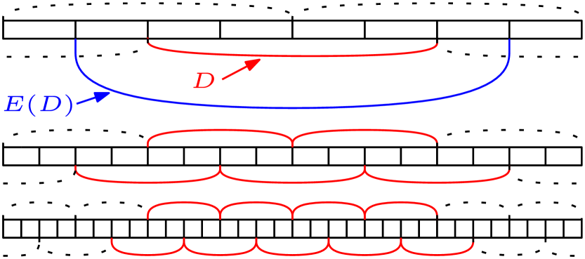
Figure 1: A quadruple $D$ and its extent $E(D)$. Quadruples that overlap $D$ at lower levels (shown in red) are fully contained in the extent $E(D)$.

Figure 2: Example of $\mathsf{A}$ for the case where $k=2$, as well as other notational definitions.

References

- [1] Belazzougui, D., Gagie, T., Munro, J.I., Navarro, G., Nekrich, Y.: Range majorities and minorities in arrays. CoRR abs/1606.04495 (2016)
- [2] Belazzougui, D., Gagie, T., Navarro, G.: Better space bounds for parameterized range majority and minority. In: Proc. WADS 2013. LNCS, vol. 8037, pp. 121–132. Springer (2013)
- [3] Boyer, R.S., Moore, J.S.: MJRTY: A fast majority vote algorithm. In: Automated Reasoning: Essays in Honor of Woody Bledsoe. pp. 105–118. Automated Reasoning Series, Kluwer Academic Publishers (1991)
- [4] Chan, T.M., Durocher, S., Larsen, K.G., Morrison, J., Wilkinson, B.T.: Linear-space data structures for range mode query in arrays. Theory Comput. Syst. 55(4), 719–741 (2014)
- [5] Demaine, E.D., López-Ortiz, A., Munro, J.I.: Frequency estimation of internet packet streams with limited space. In: Proc. ESA 2002. LNCS, vol. 2461, pp. 348–360. Springer (2002)
- [6] Durocher, S., He, M., Munro, J.I., Nicholson, P.K., Skala, M.: Range majority in constant time and linear space. Inf. Comput. 222, 169–179 (2013)
- [7] Ferragina, P., Manzini, G., Mäkinen, V., Navarro, G.: Compressed representations of sequences and full-text indexes. ACM Trans. Algorithms 3(2), 20 (2007)
- [8] Ferragina, P., Venturini, R.: A simple storage scheme for strings achieving entropy bounds. Theor. Comput. Sci. 372(1), 115–121 (2007)
- [9] Gagie, T., He, M., Munro, J.I., Nicholson, P.K.: Finding frequent elements in compressed 2d arrays and strings. In: Proc. SPIRE 2011. LNCS, vol. 7024, pp. 295–300. Springer (2011)
- [10] González, R., Navarro, G.: Statistical encoding of succinct data structures. In: Proc. CPM 2006. LNCS, vol. 4009, pp. 294–305. Springer (2006)
- [11] Grossi, R., Gupta, A., Vitter, J.S.: High-order entropy-compressed text indexes. In: Proc. SODA 2003. pp. 841–850. ACM/SIAM (2003)
- [12] Karp, R.M., Shenker, S., Papadimitriou, C.H.: A simple algorithm for finding frequent elements in streams and bags. ACM Trans. Database Syst. 28, 51–55 (2003)
- [13] Karpinski, M., Nekrich, Y.: Searching for frequent colors in rectangles. In: Proc. CCCG 2008 (2008)
- [14] Misra, J., Gries, D.: Finding repeated elements. Sci. Comput. Program. 2(2), 143–152 (1982)
- [15] Navarro, G., Thankachan, S.V.: Optimal encodings for range majority queries. Algorithmica 74(3), 1082–1098 (2016)
- [16] Patrascu, M.: Succincter. In: Proc. FOCS 2008. pp. 305–313. IEEE (2008)
- [17] Patrascu, M., Roditty, L.: Distance oracles beyond the thorup-zwick bound. SIAM J. Comput. 43(1), 300–311 (2014)
- [18] Raman, R.: Encoding data structures. In: Proc. WALCOM 2015. LNCS, vol. 8973, pp. 1–7. Springer (2015)
- [19] Raman, R., Raman, V., Satti, S.R.: Succinct indexable dictionaries with applications to encoding k-ary trees, prefix sums and multisets. ACM Trans. Algorithms 3(4), 43 (2007)
- [20] Skala, M.: Array range queries. In: Space-Efficient Data Structures, Streams, and Algorithms - Papers in Honor of J. Ian Munro on the Occasion of His 66th Birthday. LNCS, vol. 8066, pp. 333–350. Springer (2013)