Flavour composition and entropy increase of cosmological neutrinos after decoherence

Abstract

We propose that gravitational interactions of cosmic neutrinos with the statistically homogeneous and isotropic fluctuations of space-time leads to decoherence. This working hypothesis, which we describe by means of a Lindblad operator, is applied to the system of two- and three-flavour neutrinos undergoing vacuum oscillations and the consequences are investigated. As result of this decoherence we find that the neutrino entropy would increase as a function of initial spectral distortions, mixing angles and CP-violation phase. Subsequently we discuss the chances to discover such an increase observationally (in principle). We also present the expected flavour composition of the cosmic neutrino background after decoherence is completed. The physics of two- or three-flavour oscillation of cosmological neutrinos resembles in many aspects two- or three-level systems in atomic clocks, which were recently proposed by Weinberg for the study of decoherence phenomena.

1 Introduction

The indirect evidence for the existence of a cosmic neutrino background (CNB) is a major achievement of observational cosmology [1, 2, 3]. Its direct detection remains an experimental challenge [4, 5].

Active neutrinos are in thermal equilibrium in the early Universe. Their momentum spectra follow the Fermi-Dirac distribution, which is preserved after their decoupling — even after they became non-relativistic. Non-instantaneous decoupling and neutrino heating by electron-positron annihilation introduce distortions to the perfect Fermi-Dirac spectrum for each neutrino flavour [6, 7]. These spectral distortions are smoothed out by neutrino oscillations, but do not disappear completely. These distortions in the neutrino spectra imply a small increase of the neutrino density, giving $N_{\rm eff}=3.046$ in terms of effective number of neutrinos. In order to arrive at this result, one assumes that there are no primordial lepton-flavour asymmetries.

In this work we study the cosmic evolution and decoherence (i.e., the irreversible loss of quantum coherence) of active neutrino flavours from their decoupling (when the Universe had a temperature of $\sim 1$ MeV) to the present time. We ask the question what happens to the neutrino mass states when they become non-relativistic at late times. We propose in this work that the neutrino mass states undergo decoherence when the heaviest and second heaviest states become non-relativistic. The reasoning behind this hypothesis is that mass states in the non-relativistic regime have very different group velocities and therefore travel on different paths in space-time. The isotropic and homogeneous universe described by the $\Lambda$CDM model is homogeneous only in a statistical sense. There are fluctuations of the gravitational potential that vary in position and time. Coherent states traveling through this space-time may accumulate enough differences in their paths to reach an irreversible trajectory, causing the loss of information and the respective decoherence. Corresponding to the decoherence, a time averaging of the phase of these states traveling through different paths in space-time would also result in a break up of time reversibility. As a consequence of this hypothetical decoherence, there is an associated increase of neutrino entropy. We also present the small corrections to the flavour distribution of the CNB today, which were seeded by primordial spectral distortions.

To track the evolution of the flavour content of individual neutrinos of given momentum we make use of the Wigner density matrix in a basis $\{\left|v_{a}\right\rangle\}$

$$\rho_{p}(t)=\sum_{a,b}\left|v_{a}\rangle\rho_{ab}(p,t)\langle v_{b}\right|,$$ (1)

where the entries $\rho_{ab}(t,p)$ are defined at time $t$ and momentum $p$.

To obtain the distribution function for an ensemble of neutrinos specified by the flavour state label $\alpha$, we have to trace the projected density matrix $\rho_{p}$ and multiply by the appropriate momentum spectrum and spin degrees of freedom,

$$f_{\alpha}(p,T)=f_{\alpha}^{\rm eq}(p,T)\mathrm{tr}\left[\left|v_{\alpha}\rangle\langle v_{\alpha}\right|\rho_{p}\right],$$ (2)

where $f_{\alpha}^{\rm eq}(p,T)$ is the equilibrium momentum spectrum at temperature $T$ in which we also account for the spin degrees of freedom. The density matrix contains the flavour dependent spectral distortions, which are also momentum dependent. Since we are only interested in the flavour composition of spectral distortions, we focus on the normalized density matrix spanned by the basis $\{\left|v_{a}\right\rangle\}$. Moreover, we drop the subindex $p$ that indicates the momentum dependence for simplicity, but all the equations are momentum dependent. For the purpose of this work, the momentum dependence is trivial as the comoving momentum is conserved after neutrino decoupling.

The time evolution of the density matrix $\rho$ is given by the von Neumann equation. In an expanding Friedman-Lemaître model, after neutrino decoupling and after electron-positron annihilation (i.e. for $T<m_{e}/3\approx 0.2$ MeV), it reads

$$\imath D\rho=[{\mathcal{H}},\rho],$$ (3)

where ${\mathcal{H}}$ is the free Hamiltonian. The density matrix and the Hamiltonian are both functions of the cosmic scale factor $a$ and the modulus of the comoving neutrino momentum $q\equiv ap$. Both $\rho$ and $\mathcal{H}$ are hermitian and $\mathrm{tr}\rho=1$. The differential operator

$$D=\frac{d}{dt}=H(a)\frac{{\rm d}}{{\rm d}\ln a},$$ (4)

with $H$ denoting the Hubble expansion rate and with $a=1$ today. The cosmological redshift $z=1/a-1$.

A pure state is characterised by $\mathrm{tr}\rho^{2}=1$, while for mixed states $\mathrm{tr}\rho^{2}<1$. Thus any physical system has $\mathrm{tr}\rho^{2}\leq 1$. Since the von Neumann equation preserves $\mathrm{tr}\rho^{2}$, it cannot describe the process of decoherence. This follows as the von Neumann equation is a direct consequence of the unitary time evolution described by the Schrödinger equation.

The density matrix is connected to the (von Neumann) entropy via

$$S=-\mathrm{tr}[\rho\ln\rho].$$ (5)

The von Neumann entropy vanishes for pure states and is maximal for maximally mixed states. For a two (three) flavour state system, the maximally achievable family entropy (following Boltzmann) obviously is $S=\ln 2$ ($\ln 3$). Here we ignore the spin and momentum dependence of neutrinos. The von Neumann equation conserves this entropy and does not describe decoherence.

Here we assume that different mass states in the non-relativistic regime travel through different stochastic gravitational potentials, which leads effectively to a phase averaging. A time average along the neutrino path will consequently cause a definite decoherence. This loss of information cannot be recovered, it is not a de-phasing or kinetic decoherence that can be undone by a precise measurement. However, we will not model the different paths that the neutrino states travel and neither perform the time average, instead we will introduce a decoherence operator in the von Neumann equation encompassing the gravitational environmental fluctuations. The methodology of using an effective operator to introduce environmental sources of decoherence in an open quantum system is commonly adopted, including for neutrinos [8, 9, 10].

The modified von Neumann equation with a proper operator to describe decoherence is given by

$$\imath D\rho^{\rm L}=[{\mathcal{H}},\rho^{\rm L}]+\imath\sum_{a}\left[{\cal L}_{a},\left[\rho^{\rm L},{\cal L}_{a}\right]\right]\ ,$$ (6)

which we refer to as Lindblad equation [11]. The ${\cal L}_{a}$ are so-called Lindblad operators, arising from tracking or averaging environment dynamics. The decoherence term is responsible for the fact that the quantum system can develop dissipation and irreversibility and lose quantum coherence. As we will show shortly, the entropy for the density matrix $\rho^{\rm L}$, as well as for a time averaged density matrix over irreversible paths $\bar{\rho}$, is not constant anymore.

Many aspects of oscillating neutrinos in the early Universe have been discussed before. The focus of those works may be in the interplay with the primordial plasma [12, 13], the matter effect [7, 14], the role of a lepton asymmetry [15, 16, 17] or the back-reaction effects in primeval nucleosynthesis [18, 19]. Important for this work are studies of distortions in the neutrino spectral distribution [20, 18, 21]. These works rely on an approach similar to ours, but are not identical, especially regarding the exact solution for three-flavour oscillations in the cosmological context, with and without including Lindblad operators to account for decoherence. In [22] a spontaneous suppression operator is adopted to account for decoherence, but the focus is not the evolution of entropy. Importantly, most existing studies are concerned with the interplay of neutrino oscillations and the plasma, therefore their focus lies on the epoch of neutrino decoupling. To our knowledge, the epoch after neutrino decoupling has not been explored in great detail, especially the effect of the transition from the relativistic to non-relativistic regime in a statistically homogeneous space, which we argue is the source of decoherence proposed in this work.

Often a prescription based on wave packets is adopted to account for the process of decoherence [23, 24], e.g. for supernova neutrinos [25, 26, 27, 28] or cosmological neutrinos [29]. In the latter work it is argued that cosmological neutrinos should not be treated as a classical, collisionless fluid. The author of [30] addresses the increase of neutrino entropy due to decoherence of mixed massive neutrinos, but without solving the Lindblad equation or using wave packets. As we show below, our findings go well beyond the studies presented in [29] and [30].

Lindblad operators have been used more recently to account for various decoherence processes [31, 32, 33, 34, 35], as well as in the context of neutrino oscillations in laboratory experiments, and both for two [32, 8] and for three neutrino flavours [36, 9, 10]. However, the use of Lindblad operators for cosmological neutrinos in this work is novel, as well as the exact solution for three neutrino flavours that is valid throughout the relativistic and non-relativistic regimes.

Using Lindblad operators, one can mimic the damping of mixed states caused by a hypothetical decoherence phenomenon and predict the net change in entropy in a mathematical rigorous way. We also argue that cosmological neutrinos could be used to improve our understanding of decoherence in analogue to the recently proposed studies of decoherence in atomic clocks [34].

This work is structured as follows. In the next two sections we present exact solutions for two- and three-flavour neutrino oscillations in cosmology, including decoherence. We show that suitable Lindblad operators give rise to decoherence and that time averaging would lead to the same result for the asymptotic density matrix, we discuss the validity and generality of this result. In section 4 we study the increase of family entropy associated with decoherence. We conclude with a discussion of our findings.

Whenever we use values for neutrino mixing angles and mass square differences, we use the best-fit values from [38]: $\sin^{2}\theta_{12}=0.320^{+0.016}_{-0.017}$, $\sin^{2}\theta_{23}=0.613^{+0.022}_{-0.040}(0.600^{+0.023}_{-0.031})$, $\sin^{2}\theta_{13}=0.0246^{+0.0029}_{-0.0028}(0.0250^{+0.0026}_{-0.0027})$, $\Delta m_{21}^{2}=(7.62\pm 0.19)\times 10^{-5}\text{ eV}^{2}$ and $|\Delta m_{31}^{2}|=2.55^{+0.06}_{-0.09}(2.43^{+0.07}_{-0.06})\times 10^{-3}\text{ eV}^{2}$. Where the values are for normal (inverted) hierarchy. The exception is the Dirac CP-violation phase which we set to zero for the sake of simplicity, although we explore its effect in the appendix A. The best-fit value for the CP-violation phase is $0.8\pi(-0.03\pi)$, but the phase is not measured at statically significant level. The convention adopted on the mixing angles follows the standard of the Particle Data Group [37]. The neutrino oscillation parameters adopted here have been obtained from neutrino oscillation experiments only [38] and are in agreement with an independent recent compilation [39], that also uses cosmological information.

2 Neutrino oscillations: two-flavour case

We start by a discussion of the two-flavour case. Although some readers might think that this is a trivial exercise, we think that it is useful to clarify the concepts and the method for a discussion of the three-flavour case. We obtain an exact analytic treatment of neutrino vacuum oscillations from the relativistic to the non-relativistic regime in an expanding universe, their decoherence and time and/or momentum averaging for arbitrary initial conditions, neutrino parameters and cosmological model parameters.

The physical state of a system with two neutrino flavours is described by a two-dimensional Hilbert space (factored with the corresponding spaces for the other physical degrees of freedom — neutrino spin and momentum). The space of all hermitian $2\times 2$ matrices is spanned by the unit matrix $I$ and the Pauli matrices $\sigma_{i}$, where the Latin indices $i$ run from $1$ to $3$. We write for any hermitian matrix $M=M_{0}I+M_{i}\sigma_{i}$, where we sum over repeated indices. We have $\mathrm{tr}M=2M_{0}$ and $\mathrm{tr}M^{2}=2(M_{0}^{2}+M_{i}^{2})$. Note that hermiticity implies that the components $M_{i}$ are real numbers.

Expressing the density matrix in this matrix basis, the von Neumann equation (3) becomes

$$D\rho_{0}=0,\quad D\rho_{i}=2\epsilon_{ijk}\mathcal{H}_{j}\rho_{k},$$ (7)

with $\epsilon_{ijk}$ denoting the totally antisymmetric symbol. The trace condition gives $\rho_{0}=1/2$.

So far we did not specify a basis for the neutrino states. The free Hamiltonian is diagonal for the neutrino mass states and reads

$$\mathcal{H}_{\rm m}=\mathcal{H}_{0}I+\mathcal{H}_{3}\sigma_{3},$$ (8)

with

$$\mathcal{H}_{0} = \frac{1}{2}\left(\sqrt{m_{1}^{2}+\frac{q^{2}}{a^{2}}}+\sqrt{m_{2}^{2}+\frac{q^{2}}{a^{2}}}\right),$$ (9)

$$\mathcal{H}_{3} = \frac{1}{2}\left(\sqrt{m_{1}^{2}+\frac{q^{2}}{a^{2}}}-\sqrt{m_{2}^{2}+\frac{q^{2}}{a^{2}}}\right).$$ (10)

Without restriction of generality we assume that $0\leq m_{1}<m_{2}$. For $m_{1}=m_{2}$ we find that $\mathcal{H}_{3}=0$ and $\rho$ is a constant matrix.

Flavour mixing is described by a two dimensional rotation ($U^{\dagger}U=I$), written as

$$U=\left(\begin{array}[]{cc}\cos\theta&\sin\theta\\ -\sin\theta&\cos\theta\end{array}\right).$$ (11)

The Hamiltonian in flavour space reads:

$$\mathcal{H}_{\mathrm{f}}=U\mathcal{H}_{\mathrm{m}}U^{\dagger}.$$ (12)

Thus the solution in flavour basis is

$$\rho_{\rm f}(a,q)=U\rho_{\rm m}(a,q)U^{\dagger},$$ (13)

where the initial condition for the mass states is given by the rotated conditions in flavour space

$$\rho_{\rm m}(a_{\rm ini},q)=U^{\dagger}\rho_{\rm f}(a_{\rm ini},q)U.$$ (14)

2.1 Exact solution

Neutrino production and detection involves neutrino interactions, i.e. flavour states. Thus for both the initial conditions and the late time values of $\rho$ we are interested in the flavour basis. Nevertheless, the Hamiltonian is diagonal in the mass basis, giving rise to simple time evolution of equation (3). We thus first study the time evolution in the mass basis using Bloch vectors. Once the time evolution is known, we can specify the initial conditions in flavour basis, transform them to the mass basis, evolve in time and finally transform back to the flavour basis. As shown below, this can be done analytically without any assumption on neutrino masses, momenta or cosmological model.

In the mass basis the von Neumann equation (7) is simply,

$$D\rho_{0}=0,\quad D\rho_{1}=-2\mathcal{H}_{3}\rho_{2},\quad D\rho_{2}=2\mathcal{H}_{3}\rho_{1},\quad D\rho_{3}=0.$$ (15)

Thus $\rho_{0}$ and $\rho_{3}$ are constants. Furthermore, we define

$$\Delta(a,q)=-2\mathcal{H}_{3}=\left(\sqrt{m_{2}^{2}+\frac{q^{2}}{a^{2}}}-\sqrt{m_{1}^{2}+\frac{q^{2}}{a^{2}}}\right).$$ (16)

With the new variable

$${\rm d}x_{q}=\frac{\Delta(a,q)}{H(a)}{\rm d}\ln a,$$ (17)

we find the exact solution

$$\rho_{1}(x)=A_{q}\cos(x_{q}+\phi_{q}),\quad\rho_{2}(x)=-A_{q}\sin(x_{q}+\phi_{q}),$$ (18)

where $A_{q}$ and $\phi_{q}$ are to be fixed by the initial conditions. We find that ${\rm tr}\rho^{2}=1/2+2(\rho_{3}^{2}+A_{q}^{2})$.

As we saw already, the first necessary condition for neutrino oscillation (a non-trivial evolution of the density matrix) is $m_{2}>m_{1}$. A second necessary condition is $\theta\neq 0$, as for $\theta=0$ the mass basis agrees with the flavour basis and only non-trivial values for $\rho_{0}$ and $\rho_{3}$ could be generated (under the assumption that neutrinos can only be generated in a pure flavour state). As was shown above, both $\rho_{0}$ and $\rho_{3}$ are preserved in the mass basis and thus for vanishing mixing angles no neutrino oscillations occur.

As we show below, there is also a third necessary condition for the oscillations of neutrino flavours to happen: at least one of the $\rho_{{\rm f}i}\neq 0$, otherwise the oscillation amplitude $A$ vanishes.

In order to find explicit expressions we first study how the Pauli matrices are transformed from mass to flavour space. The transformation in the other direction is obtained by $\theta\to-\theta$. This allows us to fix the constants $A_{q}$ and $\phi_{q}$. In the following we drop the explicit indication of the $q$-dependence; we find

$$A=\sqrt{[\cos(2\theta)\rho_{{\rm f}1}(x_{\rm ini})+\sin(2\theta)\rho_{{\rm f}3}(x_{\rm ini})]^{2}+\rho_{{\rm f}2}(x_{\rm ini})^{2}}$$ (19)

and

$$\phi=-x_{\rm ini}+\arctan\left(\frac{-\rho_{{\rm f}2}(x_{\rm ini})}{\cos(2\theta)\rho_{{\rm f}1}(x_{\rm ini})+\sin(2\theta)\rho_{{\rm f}3}(x_{\rm ini})}\right).$$ (20)

Finally, at $x>x_{\rm ini}$, we may express the most general solution in flavour space as

$$\rho_{{\rm f}0}(x) = \frac{1}{2},$$ (21)

$$\rho_{{\rm f}1}(x) = \cos(2\theta)A\cos(x+\phi)+\sin^{2}(2\theta)\rho_{{\rm f}1}(x_{\rm ini})-\sin(2\theta)\cos(2\theta)\rho_{{\rm f}3}(x_{\rm ini}),$$ (22)

$$\rho_{{\rm f}2}(x) = -A\sin(x+\phi),$$ (23)

$$\rho_{{\rm f}3}(x) = \sin(2\theta)A\cos(x+\phi)-\sin(2\theta)\cos(2\theta)\rho_{{\rm f}1}(x_{\rm ini})+\cos^{2}(2\theta)\rho_{{\rm f}3}(x_{\rm ini}).$$ (24)

It is interesting to check that indeed

$$\mathrm{tr}\rho^{2}=\frac{1}{2}+2[\rho_{{\rm f}1}^{2}(x_{\rm ini})+\rho_{{\rm f}2}^{2}(x_{\rm ini})+\rho_{{\rm f}3}^{2}(x_{\rm ini})]$$ (25)

is a preserved quantity. As $\mathrm{tr}\rho^{2}\leq 1$ for any physical state, we find that the initial conditions have to satisfy the constraint

$$\rho_{{\rm f}1}^{2}(x_{\rm ini})+\rho_{{\rm f}2}^{2}(x_{\rm ini})+\rho_{{\rm f}3}^{2}(x_{\rm ini})\leq\frac{1}{4}.$$ (26)

Since the components $\rho_{i}$ are real, it follows that all individual components have to come from the interval $[-1/2,+1/2]$, for any initial conditions including arbitrary lepton-flavour asymmetries. Thus we also see that $\mathrm{tr}\rho^{2}\geq 1/2$.

For the special case of maximal mixing, given by $\theta=\pi/4$, we find

$$\rho_{{\rm f}0}(x) = \frac{1}{2},$$ (27)

$$\rho_{{\rm f}1}(x) = \rho_{{\rm f}1}(x_{\rm ini}),$$ (28)

$$\rho_{{\rm f}2}(x) = -A\sin(x-\phi),$$ (29)

$$\rho_{{\rm f}3}(x) = A\cos(x-\phi).$$ (30)

with

$$A=\sqrt{\rho_{{\rm f}3}^{2}+\rho_{{\rm f}2}^{2}},\quad\phi=-x_{\rm ini}+\arctan\left(-\frac{\rho_{{\rm f}2}(x_{\rm ini})}{\rho_{{\rm f}3}(x_{\rm ini})}\right).$$ (31)

2.2 Initial conditions

If at the initial time all neutrinos are in one of the two flavour states, we have

$$\rho_{\rm f}(x_{\rm ini})=\frac{1}{2}\left(\begin{array}[]{cc}1+\delta&0\\ 0&1-\delta\end{array}\right),$$ (32)

with $\delta=\delta(q)\in[-1,1]$ describing the asymmetry of the initial flavours. This means we assume that nature does not produce flavour-entangled (mixed) states at neutrino decoupling. Expanding in Pauli matrices

$$\rho_{{\rm f}0}(x_{\rm ini})=\frac{1}{2},\ \rho_{{\rm f}1}(x_{\rm ini})=0,\ \rho_{{\rm f}2}(x_{\rm ini})=0,\ \rho_{{\rm f}3}(x_{\rm ini})=\frac{\delta}{2},$$ (33)

and replacing in (19) and (20), we have

$$A=\frac{\delta}{2}\sin(2\theta),\quad\phi=-x_{\rm ini},$$ (34)

and finally

$$\rho_{{\rm f}0}(x) = \frac{1}{2},$$ (35)

$$\rho_{{\rm f}1}(x) = \frac{\delta}{2}[\sin(2\theta)\cos(2\theta)\cos(x-x_{\rm ini})-\sin(2\theta)\cos(2\theta)],$$ (36)

$$\rho_{{\rm f}2}(x) = -\frac{\delta}{2}\sin(2\theta)\sin(x-x_{\rm ini}),$$ (37)

$$\rho_{{\rm f}3}(x) = \frac{\delta}{2}[\sin^{2}(2\theta)\cos(x-x_{\rm ini})+\cos^{2}(2\theta)].$$ (38)

In the following we choose $x_{\rm ini}=0$, without restriction of generality.

2.3 Decoherence

To describe the decoherence of a system of two neutrino flavours in vacuum in an expanding Universe, we make use of a single Lindblad operator [32] and decompose it in Pauli matrices

$${\cal L}=l_{0}\bm{I}+\sum_{i}l_{i}\sigma_{i}\ ,$$ (39)

where we have in principle four amplitudes $l_{i}$. Any Lindblad operator ${\cal L}_{a}$ has to be hermitian (${\cal L}^{\dagger}={\cal L}$) to guarantee a monotonic increase of the von Neumann entropy and it has to commute with the Hamiltonian ($[{\cal H}_{m},{\cal L}]=0$) in order to conserve the statistical average energy $\left(\frac{d}{dt}{\rm tr}({\cal H}_{m}\rho^{\rm L})=0\right)$. Commutation with the diagonal Hamiltonian (in the mass basis in vacuum) requires that $l_{1}=l_{2}=0$, resulting in the decoherence operator

$$\left[{\cal L},\left[\rho^{\rm L},{\cal L}\right]\right]=-4l_{3}^{2}(\sigma_{1}\rho_{1}^{\rm L}+\sigma_{2}\rho_{2}^{\rm L})\ .$$ (40)

Without restriction of generality we put $l_{0}=0$, as it does not show up in the Lindblad equation. Thus, the components of the master equation with the Lindblad operator ${\cal L}$ become

$$D\rho^{\rm L}_{0}=0,\quad D\rho^{\rm L}_{1}=-2\mathcal{H}_{3}\rho^{\rm L}_{2}-4l_{3}^{2}\rho^{\rm L}_{1},\quad D\rho^{\rm L}_{2}=2\mathcal{H}_{3}\rho^{\rm L}_{1}-4l_{3}^{2}\rho^{\rm L}_{2},\quad D\rho^{\rm L}_{3}=0,$$ (41)

whose solution in mass basis can also be found analytically (using $dt=-dx/2{\cal H}_{3}$),

$$\rho^{\rm L}_{0}(x) = \frac{1}{2},$$ (42)

$$\rho^{\rm L}_{1}(x) = \frac{\delta}{2}\sin(2\theta)\cos(x)\exp\left[{2\int\frac{l_{3}^{2}}{\mathcal{H}_{3}}dx}\right],$$ (43)

$$\rho^{\rm L}_{2}(x) = -\frac{\delta}{2}\sin(2\theta)\sin(x)\exp\left[{2\int\frac{l_{3}^{2}}{\mathcal{H}_{3}}dx}\right],$$ (44)

$$\rho^{\rm L}_{3}(x) = \frac{\delta}{2}\cos(2\theta),$$ (45)

and are easily rotated to the flavour basis

$$\rho^{\rm L}_{{\rm f}0}(x) = \frac{1}{2},$$ (46)

$$\rho^{\rm L}_{{\rm f}1}(x) = -\frac{\delta}{2}\sin(2\theta)\cos(2\theta)\left(1-\cos(x)\exp\left[{2\int\frac{l_{3}^{2}}{\mathcal{H}_{3}}dx}\right]\right),$$ (47)

$$\rho^{\rm L}_{{\rm f}2}(x) = -\frac{\delta}{2}\sin(2\theta)\sin(x)\exp\left[{2\int\frac{l_{3}^{2}}{\mathcal{H}_{3}}dx}\right],$$ (48)

$$\rho^{\rm L}_{{\rm f}3}(x) = \frac{\delta}{2}\left(\cos^{2}(2\theta)+\sin^{2}(2\theta)\cos(x)\exp\left[{2\int\frac{l_{3}^{2}}{\mathcal{H}_{3}}dx}\right]\right).$$ (49)

Note that $l_{3}$ can be an arbitrary real function of $x_{q}$. The integral in the exponent is negative definite if $l_{3}\neq 0$ and thus gives rise to a damping of all non-diagonal components in the mass basis. We interpret the function $l_{3}(x)$ as the influence of the environment, the expanding cosmos, that leads to the decoherence of neutrino states.

2.4 Averaging

The time averaging of (35) – (38) produces the same asymptotic result as the decoherence process by the Lindblad operator. The final effect is the suppression of terms with time dependence. For time averaging the fast oscillations terms take asymptotic values ($\langle\cos(x)\rangle=\langle\sin(x)\rangle\rightarrow 0$ and $\langle\sin^{2}(x)\rangle=\langle\cos^{2}(x)\rangle\rightarrow 1/2$). Using Lindblad operators, one can see that the terms which have a time dependence in the mass basis, equations (43) and (44), are exponentially suppressed once decoherence starts, extinguishing the off-diagonal contributions corresponding to mixed states. In the flavour basis, the off-diagonal terms are driven to a constant value. We use the effect of the Lindblad operator to describe decoherence, setting to zero the contributions from $\rho_{1}$ and $\rho_{2}$ in the mass basis and then rotate to the flavour basis

$$\bar{\rho}_{{\rm f}0} = \frac{1}{2},$$ (50)

$$\bar{\rho}_{{\rm f}1} = -\sin(2\theta)\cos(2\theta)\frac{\delta}{2},$$ (51)

$$\bar{\rho}_{{\rm f}2} = 0,$$ (52)

$$\bar{\rho}_{{\rm f}3} = \cos^{2}(2\theta)\frac{\delta}{2}.$$ (53)

For this averaged system we have $\mathrm{tr}\bar{\rho}^{2}=\frac{1}{2}[1+\delta^{2}\cos^{2}(2\theta)]$, which is independent of time or oscillation phase since we performed averaging and it depends on the mixing angle because it undergoes mixing. The result is numerically equivalent to a system that lost all coherence. For the exact, non-averaged solution we have $\mathrm{tr}\rho^{2}=\frac{1}{2}(1+\delta^{2})$, which is independent of mixing angles and time, as one expects for a system that undergoes unitary (deterministic) time evolution. The difference of the traces of the squared matrices, a measure for the difference of coherence of averaged and microscopic states, is then $\mathrm{tr}\bar{\rho}^{2}-\mathrm{tr}\rho^{2}=-\frac{1}{2}\delta^{2}\sin^{2}(2\theta)$.

For maximal mixing ($\theta=\pi/4$), the time averaged solution with arbitrary initial condition becomes

$$\bar{\rho}_{{\rm f}0}=1/2,\ \bar{\rho}_{{\rm f}1}=\rho_{{\rm f}1}(x_{\rm ini}),\ \bar{\rho}_{{\rm f}2}=0,\ \bar{\rho}_{{\rm f}3}=0.$$ (54)

Thus the density matrix of maximally mixing neutrinos does not depend on the mixing of the initial flavour distortion. The probabilities to find a neutrino in the first or second flavour state are equal, and the amount of mixing is constant. For initial conditions in which the neutrinos are in pure flavour states ($\rho_{{\rm f}1}(x_{i})=0$), the time averaged density matrix is proportional to the unit matrix, as one would expect.

2.5 Relation of Lindblad formalism and averages

We observe that the expressions (50) – (53) are identical to the expressions (46) – (49) asymptotically ($\rho^{\rm L}_{{\rm f}i}\simeq\bar{\rho}_{{\rm f}i}$), i.e. if the oscillation phase $x$ is large enough then decoherence has happened. The averaged density matrix agrees with the microscopic density matrix after decoherence. It might be tempting to conclude that decoherence and averaging over time (or perhaps momenta) would be equivalent. This has actually be proposed in previous literature, see e.g. [32]. However, a closer investigation reveals that this is not the case.

Let us apply our calculation to experiments which test solar, reactor or atmospheric neutrinos, in order to revisit the arguments given in [32]. The neutrinos of interest in oscillation experiments are relativistic, i.e. $q\approx E$ and thus $\Delta(a,q)\approx\Delta m^{2}/2E$ (with energy $E$), and propagate in non-expanding space [$(1/H){\rm d}\ln a=dt,a=1$]. We find the oscillation phase (17) becomes

$$x_{q}=\int\frac{\Delta(a,q)}{H(a)}{\rm d}\ln a\approx\int\frac{\Delta m^{2}}{2E}dt=\frac{\Delta m^{2}}{2E}L,$$ (55)

where the distance $L$ is the distance travelled by neutrinos at the speed of light. The decoherence term becomes

$$\exp\left(4\int_{0}^{L/c}\frac{l_{3}^{2}}{2\mathcal{H}_{3}}dx\right)=\exp(-4\int_{0}^{L/c}\!\!\!l_{3}^{2}dt)\ .$$ (56)

For the analysis of neutrino oscillation experiments, one usually measures the amount of neutrinos that were emitted in one flavour and are detected in either the same or the other flavour. This corresponds to a maximal initial distortion (e.g. $\delta=1$ corresponds to $\rho(x_{\rm ini})=\left|\nu_{1}\rangle\langle\nu_{1}\right|$). The well-known result, including a decoherence term, for the probability to measure the second flavour is now easily recovered, $P_{1\to 2}(L,E)=\mbox{tr}[\left|\nu_{2}\rangle\langle\nu_{2}\right|\rho(x)]$)

$$P_{1\to 2}(L,E)=\frac{1}{2}\sin^{2}(2\theta)\left[1-\exp({-4\int_{0}^{L/c}\!\!\!l_{3}^{2}dt})\cos\left(\frac{\Delta m^{2}}{2E}L\right)\right]\ .$$ (57)

Let us compare this result with the probability obtained in a description in which wave packets instead of Lindblad operators (i.e. $l_{3}=0$) are considered to describe the process of decoherence [32, 23]. The distribution of the oscillation phase $x$ is often assumed to be a Gaussian, the phase averaged probability of flavour oscillations is then given by

$$\left\langle P_{1\to 2}\right\rangle=\int P_{1\to 2}(x)\left[\frac{1}{\sigma\sqrt{2\pi}}\exp\left(-\frac{(x-\left\langle x\right\rangle)^{2}}{2\sigma^{2}}\right)\right]dx\ ,$$ (58)

where the phase width of the wave packet is $\sigma=\sqrt{\left\langle(x-\left\langle x\right\rangle)^{2}\right\rangle}$. The integral gives

$$\langle P_{1\to 2}\rangle=\frac{1}{2}\sin^{2}(2\theta)\left(1-\exp\left(-\frac{\sigma^{2}}{2}\right)\cos(\langle x\rangle)\right)\ ,$$ (59)

with $\langle x\rangle=(\Delta m^{2}/2)\langle L/E\rangle.$ Comparing the equation above with equation (57), it has been argued that they have the same structure once we identify the decoherence term with the wave packet dispersion

$$4\int^{L/c}_{0}l_{3}^{2}dt=\frac{\sigma^{2}}{2}.$$ (60)

This result is the basis of the argued equivalence between Lindblad decoherence and Gaussian averaging [32].

However, this argument is inconsistent already at the level of mathematical assumptions. In order to go from (58) to (59), $\sigma$ was assumed to be a constant, i.e. independent of the phase $x$. But the identification (60) suggests that either $\sigma=\sigma(L)$, inconsistent with the assumption, or the integral on the l.h.s. should be constant. To make that integral a constant we can assume that $l_{3}^{2}$ is proportional to a Dirac-delta distribution on the time interval $[0,L/c]$, which would correspond to a sudden, but incomplete decoherence, i.e. the asymptotic state remains to show (damped) neutrino oscillations. We conclude that the two mechanisms, decoherence and phase (or time or momentum) averaging are not physically equivalent.

3 Neutrino oscillations: three-flavour case

For the three flavour case the space of hermitian matrices is spanned by the unit matrix and the Gell-Mann matrices $\lambda_{i}$ [40] where the index $i$ runs from 1 to 8. In this case, equation (3) becomes

$$D\rho_{0}=D\rho_{3}=D\rho_{8}=0,\quad D\rho_{k}=2f_{i3k}\rho_{i}\mathcal{H}_{3}+2f_{i8k}\rho_{i}\mathcal{H}_{8}\ ,$$ (61)

where $f_{ijk}$ are the usual structure constants of the Lie algebra su(3). By unitarity, we mandatorily have $\rho_{0}=1/3$.

In the mass basis the Hamiltonian is diagonal and is given by

$$\mathcal{H}_{\rm m}=\mathcal{H}_{0}I+\mathcal{H}_{3}\lambda_{3}+\mathcal{H}_{8}\lambda_{8},$$ (62)

with

$$\mathcal{H}_{0} = \frac{1}{3}\left(\sqrt{m_{1}^{2}+\frac{q^{2}}{a^{2}}}+\sqrt{m_{2}^{2}+\frac{q^{2}}{a^{2}}}+\sqrt{m_{3}^{2}+\frac{q^{2}}{a^{2}}}\right),$$ (63)

$$\mathcal{H}_{3} = \frac{1}{2}\left(\sqrt{m_{1}^{2}+\frac{q^{2}}{a^{2}}}-\sqrt{m_{2}^{2}+\frac{q^{2}}{a^{2}}}\right),$$ (64)

$$\mathcal{H}_{8} = \frac{1}{2\sqrt{3}}\left(\sqrt{m_{1}^{2}+\frac{q^{2}}{a^{2}}}+\sqrt{m_{2}^{2}+\frac{q^{2}}{a^{2}}}-2\sqrt{m_{3}^{2}+\frac{q^{2}}{a^{2}}}\right).$$ (65)

Without restriction of generality we assume that $0\leq m_{1}<m_{2}<m_{3}$ for normal hierarchy and $0\leq m_{3}<m_{1}<m_{2}$ for inverted hierarchy. Once again, for equal or vanishing masses the Hamiltonian is proportional to the identity matrix.

The flavour mixing matrix is now a three dimensional rotation ($U^{\dagger}U=I$) and can be written as

$$U=\left(\begin{array}[]{ccc}c_{12}c_{13}&s_{12}c_{13}&s_{13}e^{-i\delta_{\rm CP}}\\ -s_{12}c_{23}-c_{12}s_{23}s_{13}e^{i\delta_{\rm CP}}&c_{12}c_{23}-s_{12}s_{23}s_{13}e^{i\delta_{\rm CP}}&s_{23}c_{13}\\ s_{12}s_{23}-c_{12}c_{23}s_{13}e^{i\delta_{\rm CP}}&-c_{12}s_{23}-s_{12}c_{23}s_{13}e^{i\delta_{\rm CP}}&c_{23}c_{13}\end{array}\right),$$ (66)

where $c_{ij}=\cos\theta_{ij}$, $s_{ij}=\sin\theta_{ij}$ and $\delta_{\rm CP}$ is a Dirac charge-parity (CP) violating phase. In the main body of this work we assume vanishing CP-violation and include some results for a non-vanishing value in the appendix A. Both Majorana phases are irrelevant for the aspects discussed in this work. The Hamiltonian in flavour space is obtained as in equation (12).

3.1 Exact solution

While the initial states and the states observable by means of a particle physics detector are given in flavour basis, the von Neumann equation and its solution is most suitable formulated in the mass basis. This approach simplifies the system of equations since the Hamiltonian is diagonal in the mass basis,

$$D\rho_{0}=0,\ D\rho_{1}=-2\mathcal{H}_{3}\rho_{2},\ D\rho_{2}=2\mathcal{H}_{3}\rho_{1},$$

$$D\rho_{3}=0,\ D\rho_{4}=-\left(\mathcal{H}_{3}+\sqrt{3}\mathcal{H}_{8}\right)\rho_{5},\ D\rho_{5}=\left(\mathcal{H}_{3}+\sqrt{3}\mathcal{H}_{8}\right)\rho_{4},$$ (67)

$$D\rho_{6}=-\left(-\mathcal{H}_{3}+\sqrt{3}\mathcal{H}_{8}\right)\rho_{7},\ D\rho_{7}=\left(-\mathcal{H}_{3}+\sqrt{3}\mathcal{H}_{8}\right)\rho_{6},\ D\rho_{8}=0.$$

The diagonal components of the density matrix ($\rho_{0},\rho_{3}$ and $\rho_{8}$) are constant. The remaining off-diagonal components give rise to oscillating solutions. The oscillation frequency is determined by combinations of the asymmetric terms of the Hamiltonian ($\mathcal{H}_{3}$ and $\mathcal{H}_{8}$). There are six equations, forming three independent harmonic oscillators of two levels each, where their frequency is given by

$$\Delta(a,q)_{21}=-2\mathcal{H}_{3}=\left(\sqrt{m_{2}^{2}+\frac{q^{2}}{a^{2}}}-\sqrt{m_{1}^{2}+\frac{q^{2}}{a^{2}}}\right)\ ,$$ (68)

$$\Delta(a,q)_{31}=-(\mathcal{H}_{3}+\sqrt{3}\mathcal{H}_{8})=\left(\sqrt{m_{3}^{2}+\frac{q^{2}}{a^{2}}}-\sqrt{m_{1}^{2}+\frac{q^{2}}{a^{2}}}\right)\ ,$$ (69)

$$\Delta(a,q)_{32}=-(-\mathcal{H}_{3}+\sqrt{3}\mathcal{H}_{8})=\left(\sqrt{m_{3}^{2}+\frac{q^{2}}{a^{2}}}-\sqrt{m_{2}^{2}+\frac{q^{2}}{a^{2}}}\right)\ ,$$ (70)

for simplicity, we define three different oscillation phases to account for the three sectors of oscillation

$${\rm d}x_{ij}=\frac{\Delta(a,q)_{ij}}{H(a)}{\rm d}\ln a\ ,$$ (71)

where the only three independent combinations are $ij=21,31,32$. We find the exact solutions

$$\rho_{1}(x_{21})=+A\cos(x_{21}+\phi_{{12}}),\quad\rho_{2}(x_{21})=-A\sin(x_{21}+\phi_{{12}}),$$

$$\rho_{4}(x_{31})=+B\cos(x_{31}+\phi_{{45}}),\quad\rho_{5}(x_{31})=-B\sin(x_{31}+\phi_{{45}}),$$

$$\rho_{6}(x_{32})=+C\cos(x_{32}+\phi_{{67}}),\quad\rho_{7}(x_{32})=-C\sin(x_{32}+\phi_{{67}}).$$ (72)

The amplitudes $A$, $B$ and $C$ and phases $\phi_{{12}}$, $\phi_{{45}}$ and $\phi_{{67}}$ are fixed by the initial conditions. For arbitrary initial conditions, we find ${\rm tr}\rho^{2}=1/3+2(\rho_{3}^{2}+\rho_{8}^{2}+A^{2}+B^{2}+C^{2})$.

During the radiation dominated epoch all three neutrinos are relativistic and the oscillation phase can be approximated by $x_{ij}\approx 1/(\sqrt{\Omega_{\rm rad}}H_{0})\Delta m_{ij}^{2}/[q(1+z)^{2}]$. When the neutrinos become non-relativistic, the oscillation phases start to evolve differently with redshift. In figure 1 we show how the three different oscillation phases start to deviate from the phase evolution of relativistic neutrinos during the matter dominated epoch. Thus we compare to the redshift dependence of the relativistic case, $x_{ij}\approx 1/(\sqrt{\Omega_{\rm m}}H_{0})\ \Delta m_{ij}^{2}/[3q(1+z)^{3/2}]$. As can be clearly seen in the figure, at the moment when the most massive neutrino becomes non-relativistic, which happens at $z\sim 100$ for the cases considered, the phases start to evolve quite differently, until they evolve again in parallel in the non-relativistic regime. It is worth noting that the heavier the neutrinos are, the earlier the transition to the non-relativistic regime happens. In figure 1 we adopted the lightest mass state to be massless. Thus, one can infer that the transition happens at redshifts $z\gtrsim 100$.

The Gell-Mann matrices are transformed from mass to flavour space according to $U\lambda_{i}U^{\dagger}$. Instead of presenting the most general solution, we restrict our attention to initial states relevant to cosmology.

3.2 Initial conditions

Just before neutrino decoupling muon and tau neutrinos interact via neutral currents only, while electron neutrinos also experience charge current interactions. Thus the muon and tau neutrinos are expected to decouple slightly before the electron neutrinos [41, 18]. Neutrino oscillations started in the early Universe slightly before their decoupling (defined as the moment when the interaction rate equals the Hubble expansion rate) from the primordial plasma. Non-instantaneous decoupling and quantum electro-dynamical corrections lead to spectral distortions. At this stage, the universe was filled with free electrons and positrons but not anymore with muons or taus, which had long annihilated or decayed to lighter leptons or photons. Thus electron neutrinos end up with a different distortion of momentum and total number density than the other two active flavours. Later, during electron-positron annihilation, extra distortions are produced and again with different branching ratios for electron neutrinos and muon/tau neutrinos.

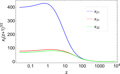
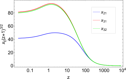
Figure 1: Evolution of the neutrino oscillation phases ($x_{21}$, $x_{31}$ and $x_{32}$) as a function of cosmological redshift $z$ for the three Gell-Mann blocks for normal (left) and inverted (right) hierarchy with the lightest mass state assumed to be massless, shown for neutrinos at the peak of their thermal distribution ($q=3.15T_{\nu}$). The mass-squared differences are inferred from the global analysis of neutrino oscillation data [38].

We assume that electron neutrinos are created with a distortion in the density matrix denoted by $\delta(q)$ and that muon and tau neutrinos can be described by the same distortion, $-\delta(q)/2$. We further allow for a difference in the spectral distortion of muon and tau neutrinos described by $\beta=\beta(q)$. Without primordial lepton-flavour asymmetry we would expect that $\beta=0$.

Without loss of generality we start to count oscillations at the moment when we set the initial conditions and thus have $x_{21}(t_{\rm ini})=x_{31}(t_{\rm ini})=x_{32}(t_{\rm ini})=0$. The assumption of pure initial flavour states gives then $\phi_{21}=\phi_{31}=\phi_{32}=0$. The initial conditions are

$$\rho_{\rm f}(0)=\frac{1}{3}\left(\begin{array}[]{ccc}1+\delta&0&0\\ 0&1-\delta/2+\beta&0\\ 0&0&1-\delta/2-\beta\end{array}\right),$$ (73)

with $\delta\in[-1,2],\beta\in[-\alpha,\alpha]$, with $\alpha=\sqrt{3-3\delta^{2}/4}$ from the condition $\mbox{tr}\rho^{2}\leq 1$. Setting the off-diagonal initial condition null is equivalent to assume that nature does not produce flavour entangled states, which is an approximation since neutrinos decoupling is not instantaneous.

Using the above initial conditions in the equations (3.1), we are left with the following initial values for the density matrix in flavour basis (spanned by Gell-Mann matrices)

$$\rho_{{\rm f}0}(0)=\frac{1}{3},\quad\rho_{{\rm f}3}(0)=\frac{1}{12}(3\delta-2\beta),\quad\rho_{{\rm f}8}(0)=\frac{1}{4\sqrt{3}}\left(\delta+2\beta\right),$$ (74)

where unshown entries are null. Rotating to the mass basis, we obtain an exact solution of the von Neumann equation for the Gell-Mann coefficients of the density matrix,

$$\rho_{{\rm}0}=\frac{1}{3},$$ (75)

$$\rho_{{\rm}1}(x_{21})=\frac{\delta}{4}\sin(2\theta_{12})\cos^{2}\theta_{13}\cos(x_{21})$$

$$+\frac{\beta}{12}\left[\sin(2\theta_{12})(\cos(2\theta_{13})-3)\cos(2\theta_{23})-4\cos(2\theta_{12})\sin\theta_{13}\sin(2\theta_{23})\right]\cos(x_{21}),$$ (76)

$$\rho_{{\rm}2}(x_{21})=-\frac{1}{4}\delta\sin(2\theta_{12})\cos^{2}\theta_{13}\sin(x_{21})$$

$$-\frac{\beta}{12}\left[\sin(2\theta_{12})(\cos(2\theta_{13})-3)\cos(2\theta_{23})-4\cos(2\theta_{12})\sin\theta_{13}\sin(2\theta_{23})\right]\sin(x_{21}),$$ (77)

$$\rho_{{\rm}3}=\frac{\delta}{4}\cos(2\theta_{12})\cos^{2}\theta_{13}$$

$$+\frac{\beta}{12}\left[\cos(2\theta_{12})(\cos(2\theta_{13})-3)\cos(2\theta_{23})+4\sin(2\theta_{12})\sin\theta_{13}\sin(2\theta_{23})\right],$$ (78)

$$\rho_{{\rm}4}(x_{31})=\frac{\delta}{4}\cos\theta_{12}\sin(2\theta_{13})\cos(x_{31})$$

$$+\frac{\beta}{6}\left[\cos\theta_{12}\sin(2\theta_{13})\cos(2\theta_{23})-2\sin\theta_{12}\cos\theta_{13}\sin(2\theta_{23})\right]\cos(x_{31}),$$ (79)

$$\rho_{{\rm}5}(x_{31})=-\frac{\delta}{4}\cos\theta_{12}\sin(2\theta_{13})\sin(x_{31})$$

$$-\frac{\beta}{6}\left[\cos\theta_{12}\sin(2\theta_{13})\cos(2\theta_{23})-2\sin\theta_{12}\cos\theta_{13}\sin(2\theta_{23})\right]\sin(x_{31}),$$ (80)

$$\rho_{{\rm}6}(x_{32})=+\frac{\delta}{4}\sin\theta_{12}\sin(2\theta_{13})\cos(x_{32})$$

$$+\frac{\beta}{6}\left[\sin\theta_{12}\sin(2\theta_{13})\cos(2\theta_{23})+2\cos\theta_{12}\cos\theta_{13}\sin(2\theta_{23})\right]\cos(x_{32}),$$ (81)

$$\rho_{{\rm}7}(x_{32})=-\frac{\delta}{4}\sin\theta_{12}\sin(2\theta_{13})\sin(x_{32})$$

$$-\frac{\beta}{6}\left[\sin\theta_{12}\sin(2\theta_{13})\cos(2\theta_{23})+2\cos\theta_{12}\cos\theta_{13}\sin(2\theta_{23})\right]\sin(x_{32}),$$ (82)

$$\rho_{{\rm}8}=+\frac{\delta}{8\sqrt{3}}\left(3\cos(2\theta_{13})-1\right)+\frac{\beta}{2\sqrt{3}}\cos^{2}(\theta_{13})\cos(2\theta_{23}),$$ (83)

where the coefficients $\rho_{{\rm}0}$, $\rho_{{\rm}3}$ and $\rho_{{\rm}8}$ are time-independent. The corresponding result including non-vanishing CP-violation phase is shown in the appendix.

We do not present the general expressions in the flavour basis because they are lengthy and for the purpose of calculating solutions after decoherence, the solution in mass basis is all we need. Instead we restrict our presentation to the case of the normal neutrino hierarchy with vanishing Dirac CP-violation phase and for the best-fit values of the mixing angles from neutrino oscillation data,

$$\rho_{{\rm f}0}(x_{ij}) = 1/3,$$ (84)

$$\rho_{{\rm f}1}(x_{ij}) = \delta[-0.08223+0.02458\cos(x_{21})+0.03569\cos(x_{31})+0.02198\cos(x_{32})]+$$ (85)

$$\beta[-0.02451+0.00191\cos(x_{21})-0.10673\cos(x_{31})+0.12933\cos(x_{32})],$$

$$\rho_{{\rm f}2}(x_{ij}) = \delta[-0.13978\sin(x_{21})-0.04476\sin(x_{31})-0.01588\sin(x_{32})]+$$ (86)

$$\beta[-0.01086\sin(x_{21})+0.13389\sin(x_{31})-0.09345\sin(x_{32})],$$

$$\rho_{{\rm f}3}(x_{ij}) = \delta[0.08141+0.14924\cos(x_{21})+0.03054\cos(x_{31})-0.01119\cos(x_{32})]+$$ (87)

$$\beta[-0.02108+0.01159\cos(x_{21})-0.09134\cos(x_{31})-0.06584\cos(x_{32})],$$

$$\rho_{{\rm f}4}(x_{ij}) = \delta[0.03797-0.08378\cos(x_{21})+0.03559\cos(x_{31})+0.01022\cos(x_{32})]+$$ (88)

$$\beta[0.05279-0.00651\cos(x_{21})-0.10645\cos(x_{31})+0.06016\cos(x_{32})],$$

$$\rho_{{\rm f}5}(x_{ij}) = \delta[0.17592\sin(x_{21})-0.02833\sin(x_{31})-0.01986\sin(x_{32})]+$$ (89)

$$\beta[0.01366\sin(x_{21})+0.08473\sin(x_{31})-0.11685\sin(x_{32})],$$

$$\rho_{{\rm f}6}(x_{ij}) = \delta[-0.09714+0.10882\cos(x_{21})-0.00012\cos(x_{31})-0.01180\cos(x_{32})]+$$ (90)

$$\beta[0.06137+0.00845\cos(x_{21})-0.00035\cos(x_{31})-0.06947\cos(x_{32})],$$

$$\rho_{{\rm f}7}(x_{ij}) = \delta[-0.03569\sin(x_{21})+0.03568\sin(x_{31})-0.03568\sin(x_{32})]+$$ (91)

$$\beta[-0.00277\sin(x_{21})-0.10673\sin(x_{31})-0.20999\sin(x_{32})],$$

$$\rho_{{\rm f}8}(x_{ij}) = \delta[0.03621+0.10009\cos(x_{21})-0.02463\cos(x_{31})+0.03268\cos(x_{32})]+$$ (92)

$$\beta[0.01492+0.00777\cos(x_{21})+0.07368\cos(x_{31})+0.19230\cos(x_{32})].$$

3.3 Decoherence

Similar to the two-flavour case, the Lindblad operator for the three-flavour case has contributions from the the same basis elements as the Hamiltonian ($[{\cal H}_{\rm m},{\cal L}]=0$), therefore its form in Gell-Mann matrices is

$${\cal L}=l_{0}I+l_{3}\lambda_{3}+l_{8}\lambda_{8}.$$ (93)

Consequently, the decoherence term reads

$$[{\cal L},[\rho^{\rm L},{\cal L}]]=-4l_{3}^{2}(\rho_{1}^{\rm L}\lambda_{1}+\rho_{2}^{\rm L}\lambda_{2})-(l_{3}+\sqrt{3}l_{8})^{2}(\rho_{4}^{\rm L}\lambda_{4}+\rho_{5}^{\rm L}\lambda_{5})$$

$$-(l_{3}-\sqrt{3}l_{8})^{2}(\rho_{6}^{\rm L}\lambda_{6}+\rho_{7}^{\rm L}\lambda_{7}).$$ (94)

Apparently, there is no contribution of the Lindblad term to the evolution equations of $\rho_{0},\rho_{3}$ and $\rho_{8}$, which thus remain constant in the mass basis. As above, we set $l_{0}=0$. The Lindblad equation (3.1) can be written as

$$D\rho_{0}^{\rm L} = 0,$$

$$D\rho_{1}^{\rm L} = -2\mathcal{H}_{3}\rho_{2}^{\rm L}-4l_{3}^{2}\rho_{1}^{\rm L},$$

$$D\rho_{2}^{\rm L} = 2\mathcal{H}_{3}\rho_{1}^{\rm L}-4l_{3}^{2}\rho_{2}^{\rm L},$$

$$D\rho_{3}^{\rm L} = 0,$$

$$D\rho_{4}^{\rm L} = -\left(\mathcal{H}_{3}+\sqrt{3}\mathcal{H}_{8}\right)\rho_{5}^{\rm L}-(l_{3}+\sqrt{3}l_{8})^{2}\rho_{4}^{\rm L},$$

$$D\rho_{5}^{\rm L} = \left(\mathcal{H}_{3}+\sqrt{3}\mathcal{H}_{8}\right)\rho_{4}^{\rm L}-(l_{3}+\sqrt{3}l_{8})^{2}\rho_{5}^{\rm L},$$ (95)

$$D\rho_{6}^{\rm L} = -\left(-\mathcal{H}_{3}+\sqrt{3}\mathcal{H}_{8}\right)\rho_{7}^{\rm L}-(l_{3}-\sqrt{3}l_{8})^{2}\rho_{6}^{\rm L},$$

$$D\rho_{7}^{\rm L} = \left(-\mathcal{H}_{3}+\sqrt{3}\mathcal{H}_{8}\right)\rho_{6}^{\rm L}-(l_{3}-\sqrt{3}l_{8})^{2}\rho_{7}^{\rm L},$$

$$D\rho_{8}^{\rm L} = 0.$$

Its solution in mass basis acquires the following decaying modes

$$\rho_{{\rm}1}^{\rm L}(x_{21}) = \rho_{{\rm}1}(x_{21})\exp\left[{4\int\frac{l_{3}^{2}}{2\mathcal{H}_{3}}dx_{21}}\right],$$ (96)

$$\rho_{{\rm}2}^{\rm L}(x_{21}) = \rho_{{\rm}2}(x_{21})\exp\left[{4\int\frac{l_{3}^{2}}{2\mathcal{H}_{3}}dx_{21}}\right],$$ (97)

$$\rho_{{\rm}4}^{\rm L}(x_{31}) = \rho_{{\rm}4}(x_{31})\exp\left[{\int\frac{(l_{3}+\sqrt{3}l_{8})^{2}}{\mathcal{H}_{3}+\sqrt{3}\mathcal{H}_{8}}dx_{31}}\right],$$ (98)

$$\rho_{{\rm}5}^{\rm L}(x_{31}) = \rho_{{\rm}5}(x_{31})\exp\left[{\int\frac{(l_{3}+\sqrt{3}l_{8})^{2}}{\mathcal{H}_{3}+\sqrt{3}\mathcal{H}_{8}}dx_{31}}\right],$$ (99)

$$\rho_{{\rm}6}^{\rm L}(x_{32}) = \rho_{{\rm}6}(x_{32})\exp\left[{\int\frac{(l_{3}-\sqrt{3}l_{8})^{2}}{-\mathcal{H}_{3}+\sqrt{3}\mathcal{H}_{8}}dx_{32}}\right],$$ (100)

$$\rho_{{\rm}7}^{\rm L}(x_{32}) = \rho_{{\rm}7}(x_{32})\exp\left[{\int\frac{(l_{3}-\sqrt{3}l_{8})^{2}}{-\mathcal{H}_{3}+\sqrt{3}\mathcal{H}_{8}}dx_{32}}\right],$$ (101)

where the first terms on the right side are identical to the solutions without the Lindblad operator, as in equations (76) – (82). The terms $\rho_{{\rm}0}$, $\rho_{{\rm}3}$ and $\rho_{{\rm}8}$ are constants and equal to their initial condition given by equations (75), (3.2) and (83).

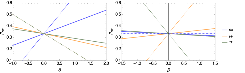
Figure 2: Probabilities to find cosmological neutrinos at different flavour states before (dotted) and after (solid) decoherence as a function of the initial distortions $\delta=\delta(q)$ (left, $\beta$ fixed to zero) and $\beta=\beta(q)$ (right, $\delta$ fixed to zero). The initial distortion for electron neutrinos is $\delta/3$, for muon neutrinos $-\delta/6+\beta/3$, and for tau neutrinos $-\delta/6-\beta/3$. The mixing angles are given by the global fit to neutrino oscillation data [38] for the normal hierarchy and we assume a vanishing CP-violation phase.

3.4 Averaging

The procedure to obtain time-averaged solutions is identical to the two-flavour case. We consider that the Lindblad operator acts on the solutions in mass basis, suppressing the time-dependent terms of the density matrix (i.e. $\rho_{{\rm}1},\rho_{{\rm}2},\rho_{{\rm}4},\rho_{{\rm}5},\rho_{{\rm}6},\rho_{{\rm}7}\rightarrow 0$). Then the averaged density matrix in flavour basis is obtained by rotating the remaining time-independent terms (i.e. $\rho_{{\rm}0},\rho_{{\rm}3},\rho_{{\rm}8}$) to obtain expressions similar to (50) – (53).

Applying the Lindblad operator simplifies the solution in the mass basis, but the rotation to the most general flavour basis generates solutions that are again too lengthy to include here. However, we can show simple solutions using the best-fit values for the mixing angles in normal hierarchy and vanishing CP-violation

$$\bar{\rho}_{{\rm f}0} = 1/3,$$ (102)

$$\bar{\rho}_{{\rm f}1} = -0.08223\delta-0.02451\beta,$$ (103)

$$\bar{\rho}_{{\rm f}2} = 0,$$ (104)

$$\bar{\rho}_{{\rm f}3} = 0.08141\delta-0.02108\beta,$$ (105)

$$\bar{\rho}_{{\rm f}4} = 0.03797\delta+0.05279\beta,$$ (106)

$$\bar{\rho}_{{\rm f}5} = 0,$$ (107)

$$\bar{\rho}_{{\rm f}6} = -0.09714\delta+0.06137\beta,$$ (108)

$$\bar{\rho}_{{\rm f}7} = 0,$$ (109)

$$\bar{\rho}_{{\rm f}8} = 0.03621\delta+0.01492\beta.$$ (110)

This allows us to obtain the probability $P_{\alpha\alpha}$ to find a neutrino of the CNB in flavour state $\alpha$,

$$P_{ee} = \bar{\rho}_{{\rm f}0}+\bar{\rho}_{{\rm f}3}+\frac{1}{\sqrt{3}}\bar{\rho}_{{\rm f}3}=\frac{1}{3}+0.1023\delta-0.0125\beta,$$ (111)

$$P_{\mu\mu} = \bar{\rho}_{{\rm f}0}-\bar{\rho}_{{\rm f}3}+\frac{1}{\sqrt{3}}\bar{\rho}_{{\rm f}3}=\frac{1}{3}-0.0605\delta+0.0297\beta,$$ (112)

$$P_{\tau\tau} = \bar{\rho}_{{\rm f}0}-\frac{2}{\sqrt{3}}\bar{\rho}_{{\rm f}3}=\frac{1}{3}-0.0418\delta-0.0172\beta.$$ (113)

A graphical illustration of this result is provided in figure 2. It shows that todays CNB does not necessarily have a 1:1:1 mix of the three active neutrino flavours. In fact, the expected mix of neutrino flavours depends on the initial values of the spectral distortions $\delta(q)$ and $\beta(q)$. In the standard (minimal) scenario with vanishing lepton-flavour asymmetries we have $\beta\ll\delta={\cal O}(10^{-4})$ and deviations from flavour equality are tiny.

3.5 Discussion

The Lindblad operator introduces two degrees of freedom for the rate of decoherence ($l_{3}$ and $l_{8}$) but the formalism itself does not indicate when the operator should start to act. To better understand the evolution of the three-flavour system, we present the increase of the oscillation phase as a function or redshift in figure 1. We see that the phases evolve in the same way as long as the neutrinos are effectively relativistic. This may give a first hint that the decoherence of cosmological neutrinos should start when the heaviest neutrino becomes non-relativistic, as already discussed for the case of two neutrino flavours.

We have learned from the discussion of the two-flavour case, that decoherence via a (in general time and momentum dependent) Lindblad operator and averaging lead to the same asymptotic density matrix. The propagation speed of a wave packet is given by the respective group velocity. In the case of three neutrino masses we have three different group velocities, which are functions of redshift,

$$v_{{\rm g}i}(z)=\frac{q(1+z)}{\sqrt{m^{2}_{i}+q^{2}(1+z)^{2}}}.$$ (114)

In figure 3 we plot the difference of these group velocities for pairs of neutrino mass states for $q=3.15T_{\nu}$. We observe that the group velocities are identical as long as all neutrinos are relativistic. They differ when the heaviest neutrino becomes non-relativistic. Again, this suggests that coherent neutrino oscillations, as described by the von Neumann equation, take place during the relativistic neutrino propagation. Without decoherence that statement would hold until today.

One could argue that neutrino oscillations can be averaged shortly after neutrino decoupling and thus decoherence takes place in the early Universe, however it seems that there is no justification for that, as neutrinos do not scatter at $T<1$ MeV and after the annihilation of positrons and electrons the number of potential scattering partners of neutrinos drops by another factor of $10^{9}$. The fact that the oscillating phase assumes high values does not necessarily mean that averaging is due automatically, since in principle one could still recover its exact value and obtain the corresponding microscopic state and trace it back to the initial state. A mechanism able to distinguish the mass states is still necessary. We suggest here that it is the transition from the relativistic to the non-relativistic evolution that induces decoherence of cosmological neutrinos and it is the difference in the inertial mass of the different neutrino states that “couple” in a different way to space-time. In a perfectly isotropic and homogeneous space-time, the different phase and group velocities would lead to a different world lines for the three mass states, but instead of evolving as independent “classical” states, they would evolve as entangled states. We think that situation must be different when we consider that the space-time is homogeneous and isotropic in a statistical sense only. We suggest that in such a situation the entanglement of the states will probably be lost due to their (gravitational) interaction with the environment.

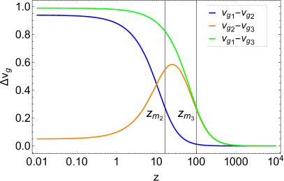
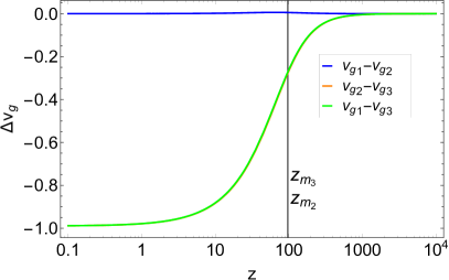
Figure 3: Difference of group velocities of neutrinos mass states for normal (left) and inverted (right) hierarchy ($m_{\rm lightest}=0$), shown for neutrinos at the peak of their thermal distribution ($q=3.15T_{\nu}$). The vertical lines mark the time of transition to the non-relativistic regime for the two massive neutrino states.

4 Entropy evolution

4.1 Two-flavour case

Let us now have a closer look at the family entropy of the system. For density matrices with $|\rho_{i}|\ll 1/2$, we approximate the von Neumann entropy, such that the logarithm can be Taylor expanded,

$$S = -\mathrm{tr}\left[\left(\frac{1}{2}I+\rho_{i}\sigma_{i}\right)\ln\left(\frac{1}{2}I+\rho_{j}\sigma_{j}\right)\right]$$ (115)

$$= \ln 2-\frac{1}{2}\mathrm{tr}\left[\left(I+2\rho_{i}\sigma_{i}\right)\ln\left(I+2\rho_{j}\sigma_{j}\right)\right]$$

$$= \ln 2-2\sum_{i=1}^{3}\rho_{i}^{2}+\mathcal{O}(4),$$

where we utilise the well-known properties of Pauli matrices, $\mathrm{tr}\sigma_{i}=0$ and $\mathrm{tr}\sigma_{i}\sigma_{j}=2\delta_{ij}$. The allowed range of initial conditions gives $\ln 2-\frac{1}{2}\leq S\leq\ln 2$ at the leading order. Presumably, higher order corrections change that into $0\leq S\leq\ln 2$.

We can also obtain an exact expression for the family entropy. In the flavour basis,

$$S=\ln 2-\frac{1}{2}(1-\delta)\ln[1-\delta]-\frac{1}{2}(1+\delta)\ln[1+\delta]\ .$$ (116)

For small initial spectral distortions, $|\delta|\ll 1$, we find

$$S(x)=\ln 2-\frac{\delta^{2}}{2}+\mathcal{O}(4).$$ (117)

Thus the family entropy is constant as quantum coherence persists as long as the neutrino oscillations are determined by the von Neumann equation.

Decoherence due to whatever reason leads to the increase of entropy. If we calculate the family entropy from the asymptotic solutions to the Lindblad equation, we find

$$S=\ln 2-\frac{1}{2}(1-\delta\cos(2\theta))\ln[1-\delta\cos(2\theta)]-\frac{1}{2}(1+\delta\cos(2\theta))\ln[1+\delta\cos(2\theta)],$$ (118)

while for small distortions

$$S=\ln 2-\cos^{2}(2\theta)\frac{\delta^{2}}{2}+\mathcal{O}\left([\cos(2\theta)\delta]^{4}\right)\ .$$ (119)

Therefore, the increase in family entropy caused by decoherence is

$$\Delta S=S_{\rm decoherent}-S_{\rm coherent}=\sin^{2}(2\theta)\frac{\delta^{2}}{2}+\mathcal{O}(\delta^{4}).$$ (120)

It is maximal for maximal mixing, which also results in the maximum entropy state. For maximal mixing and an expected spectral distortion $\delta$ of order $10^{-4}$, we find an increase of family entropy of the order of $10^{-8}$.

Let us note that the time average of the entropy without decoherence does not change, as the calculation of entropy and averaging do not commute. Thus the mathematical identity of the time averaged density matrix and the asymptotic density matrix after decoherence does not correspond to a physical equivalence of decoherence and time averaging. Nevertheless, this mathematical identity can be useful in the calculation and is exploited in this work.

4.2 Three-flavour case

The entropy for three neutrino flavours and small spectral distortions can be Taylor expanded,

$$S = -\mathrm{tr}\left[\left(\frac{1}{3}I+\rho_{i}\lambda_{i}\right)\ln\left(\frac{1}{3}I+\rho_{j}\lambda_{j}\right)\right]$$ (121)

$$= \ln 3-3\sum_{i=1}^{8}\rho_{i}^{2}+\mathcal{O}(4),$$

where we made use of $\mbox{tr}\lambda_{i}=0$ and $\mbox{tr}\lambda_{i}\lambda_{j}=2\delta_{ij}$. For the initial conditions specified in the previous section, we find the simple result

$$S=\ln 3-\frac{\delta^{2}}{4}-\frac{\beta^{2}}{3}+\mathcal{O}(4).$$ (122)

We can now calculate the increase of entropy due to decoherence. It is possible to obtain an analytical result, dependent on the mixing angles $\theta_{12}$, $\theta_{13}$, $\theta_{23}$ and the initial flavour distortions $\delta$ and $\beta$. For vanishing distortion between muon and tau neutrinos ($\beta\rightarrow 0$) there is no dependence on the angle $\theta_{23}$ or in the CP-violation phase (complete result in the appendix A). This second degree of freedom ($\beta$) is responsible for distinguishing the third-level state, without it the system becomes identical to a two-level system, when mixing between second and third state is irrelevant and it is not possible to develop CP-violation.

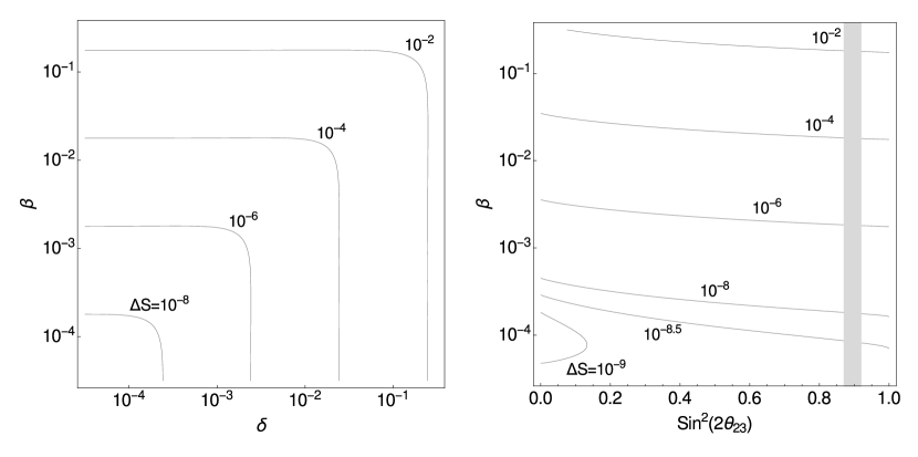
Figure 4: Family entropy increase for a system of three mixed neutrino states as functions of the initial spectral distortions $\delta$ and $\beta$ (left). The values for the mixing angles are taken from the global fit to neutrino-oscillation data [38], assuming a normal neutrino hierarchy and a vanishing Dirac CP-violation phase. In the right panel the distortion $\delta$ is set to $10^{-4}$ and the mildly constrained mixing angle $\theta_{23}$ is allowed to vary (shaded area is the allowed $3\sigma$ region).

In order to calculate the increase in flavour entropy of the neutrino due to decoherence, we make use of the fact that the von Neumann entropy does not depend on the basis in which the density matrix is given; $\mbox{tr}[\rho_{a}\ln(\rho_{a})]=\mbox{tr}[\rho_{b}\ln(\rho_{b})]$, where $(a,b)$ are different bases. We choose the most suitable basis to calculate the entropy difference of the initial (coherent) states and the final (decoherent) states,

$$\Delta S=S_{\rm decoherent}-S_{\rm coherent}=-\mbox{tr}[\bar{\rho}\ln(\bar{\rho})]+\mbox{tr}[\rho_{\rm f}(x_{\rm ini})\ln(\rho_{\rm f}(x_{\rm ini}))]\ .$$ (123)

The initial and final entropy is calculated using the flavour and mass basis, respectively, for both the density matrix is diagonal in the suitable basis. Here we exploit the mathematical identity of the asymptotic solutions for the density matrix from the Lindblad equation and the time averaged solutions of the von Neumann equation.

Although it is possible to obtain an exact solution, we choose to present an approximation for small distortions

$$\Delta S=\frac{3\delta^{2}}{64}\cos^{2}\theta_{13}\left[9-\cos(4\theta_{12})-(7+\cos(4\theta_{12}))\cos(2\theta_{13})\right]$$

$$+\frac{\beta^{2}}{192}\left[64-\cos^{2}(2\theta_{23})\left(2\cos(4\theta_{12})(\cos(2\theta_{13})-3)^{2}+12\cos(2\theta_{13})+7\cos(4\theta_{13})+37\right)\right]$$

$$-\frac{\beta^{2}}{3}\sin^{2}(2\theta_{12})\sin^{2}\theta_{13}\sin^{2}(2\theta_{23})$$

$$-\frac{\beta^{2}}{48}\sin(4\theta_{12})[\sin(3\theta_{13})-7\sin\theta_{13}]\sin(4\theta_{23})$$

$$+\frac{\beta\delta}{16}\cos^{2}\theta_{13}\cos(2\theta_{23})\left[5-(\cos(4\theta_{12})+7)\cos(2\theta_{13})+3\cos(4\theta_{12})\right]$$

$$-\frac{\beta\delta}{4}\cos^{2}\theta_{13}\sin(4\theta_{12})\sin\theta_{13}\sin(2\theta_{23})+\mathcal{O}(4)\ .$$ (124)

This is an excellent approximation up to $\delta\sim 0.5$ and, contrary to the exact solution, shows a simple dependence on the parameters.

For vanishing primordial lepton-flavour asymmetries, the special case of identical distortion for muon and tau neutrinos is theoretically well motivated. Asymmetries between these two flavours are not expected when the spectral distortions were produced. The combination of the expected initial distortion ($\delta=4.45\times 10^{-4}$, $\beta=0$) [18] with the measured mixing angles [38] gives rise to an increase of flavour entropy, $\Delta S=3.43\times 10^{-8}$. In figure 4 we present an interesting non-trivial case, when each flavour has a different distortion and we show the dependence on the only mildly constrained mixing angle $\theta_{23}$. We find that the latter affects the cosmological predictions only weakly.

5 Conclusion

In this work we have studied cosmological aspects of the decoherence of mixed neutrino states. We have described decoherence phenomena via Lindblad operators in the von Neumann equation (6).

The evolution of the family composition of the cosmic neutrino background, from the time when neutrinos are decoupled until today, has been investigated in section 3. We obtain the expected flavour composition of the CNB as a function of arbitrary initial spectral distortions, mixing angles and Dirac CP-violation phase. The net effect on the current flavour composition is shown in figure 2, where we see that neutrino oscillations and the effect of decoherence tend to equilibrate the initial flavour composition. For the measured mixing angles the equilibration is not perfect and a small residual flavour imbalance is expected. The remnant (in general momentum dependent) spectral distortion of electron neutrinos is expected to be of the order of $10^{-4}$ in the minimal scenario (no primeval lepton-flavour asymmetry).

The PTOLEMY experiment [5] is a proposal to detect cosmological neutrinos by looking for electron kinetic energies beyond the end point of the tritium $\beta$-decay spectrum [4]. According to our result, the fraction of electron neutrinos in the CNB carries information on the initial spectral distortion after $e^{\pm}$-annihilation and consequently about the state of the universe at that time. One could even speculate about futuristic detectors with such an exquisite sensitivity that even CNB intensity anisotropies [42], similar to the cosmic microwave temperature anisotropies, would be detected. The residual imbalance of neutrino flavours in the minimal scenario is one order of magnitude larger than the expected CNB anisotropies (apart from the dipole). The flavour imbalance would be increased for a lepton-flavour asymmetric universe.

We obtained exact solutions for the time-dependent Wigner density matrix, valid for any mass and momentum in a homogeneous and isotropic universe. The use of Lindblad operators results in a similar phenomenology as time-averaging for the asymptotic density matrices. We demonstrated that explicitly in section 2 for a two-flavour example.

While it is interesting that Lindblad operators and averaging give rise to the same asymptotic results for the density matrix, the time of decoherence and the details of its mechanism are not provided by the formalism used. In the three-flavour case we are left with two unknown, non-trivial and real functions, $l_{3}(x)$ and $l_{8}(x)$. In order to obtain physical intuition, we also studied the behaviour of the oscillation phase and the group velocities and their differences in figures 1 and 3. We found that the group velocities start to differ significantly once the heaviest neutrino mass state becomes non-relativistic. This suggests that the transition to the non-relativistic regime might trigger decoherence in the mass basis via the stochastic inhomogeneities of space-time, which are experienced differently by the different mass states. Subsequently neutrinos would propagate in non-degenerate mass states, which means that they are in a frozen mix of flavour states.

The problem of identifying the decoherence time can also be approached from an experimental perspective by looking for observables related to the decoherence process. Recently, a similar idea has been proposed by Weinberg [34], where he suggested that decoherence of an atomic three-level system in the context of atomic clocks could provide enough information on the time scale of decoherence that one could measure or at least constrain the Lindblad coefficients. Likewise, decoherence of cosmological neutrinos could produce a traceable observable signal by the increase of CNB entropy that immediately follows the decoherence process.

Such an entropy increase of neutrinos due to decoherence of mixed states was pointed out for supernova neutrinos [26] and for cosmological neutrinos [30] previously. The latter work assumed a fixed initial distortion proportional to the cross-section of each neutrino at the time when the oscillations started. We went beyond and considered arbitrary spectral distortions and mixing angles. To the best of our knowledge, the entropy increase with its dependence on the initial spectral distortions, mixing angles and CP-violation phase in the cosmological context is obtained for the first time. This result is valid regardless the time of when the decoherence process happens. Therefore, if we could track the CNB entropy as a function of time, we would determine the moment of neutrino decoherence observationally.

It remains to figure out how the CNB entropy could actually be measured: Since the CNB is isotropic, any increase in entropy could only manifest itself macroscopically as an induced dissipative pressure (bulk viscosity [43, 44]). Thus an entropy increase due to decoherence would affect the cosmic neutrino equation of state. Any change of the equation of state gives rise to a contribution to the integrated Sachs-Wolfe (ISW) effect. It is thus interesting to ask if such an effect could be large enough to be observable. If decoherence happens when the neutrinos become non-relativistic, i.e., when neutrinos develop different group velocities as shown in figure 3, then the decoherence contribution to the ISW effect would show up at $z\gtrsim 100$. However, we expect the effect to be tiny, since it is not only suppressed by $\delta^{2}\sim 10^{-8}$, but also by the ratio of neutrino density to matter density at $z\gtrsim 100$. Together this gives an effect of order $10^{-10}$ in the temperature anisotropies. A lepton-flavour asymmetric universe might however give rise to a larger entropy increase (see figure 4).

In this work we focused on the minimal scenario and proposed a small residual flavour imbalance of the CNB and a tiny increase of neutrino entropy at $z\sim 100$. A more detailed investigation of lepton-flavour asymmetric models might reveal useful constraints on the primeval flavour composition of the Universe.

Acknowledgments We are thankful to E. Zavanin, I. Oldengott, D. Bödeker and Y. Wong for discussions on neutrino oscillations and fruitful suggestions. We are also grateful to an anonymous referee for valuable comments and questions. DB acknowledges the financial support by CAPES-CSF, grant 8768-13-7, and by the “Bielefeld Young Researchers’ Fund”. HESV thanks CNPq and FAPES. We acknowledge the support from the RTG 1620 “Models of Gravity” funded by DFG.

Appendix A Appendix: Contribution of the CP-violation phase

In this appendix we explore results with non-vanishing CP-violation phase. The results are given in resemblance with the previous section for the three-flavour case. There is no change in the dynamics, solely in the mixing matrix. We consider the same initial conditions as in equation (73) and use the same differential equation (3.1) to obtain the results in mass basis. First, we show the solutions for each Gell-Mann block. The blocks $\lambda_{0}$, $\lambda_{3}$ and $\lambda_{8}$ are still constant

$$\rho_{{\rm}0} = \frac{1}{3},$$ (125)

$$\rho_{{\rm}3} = +\frac{\delta}{4}\cos(2\theta_{12})\cos^{2}\theta_{13}$$ (126)

$$+\frac{\beta}{12}\cos(2\theta_{12})(\cos(2\theta_{13})-3)\cos(2\theta_{23})$$

$$+\frac{\beta}{3}\sin(2\theta_{12})\sin\theta_{13}\sin(2\theta_{23})\cos(\delta_{\rm CP}),$$

$$\rho_{{\rm}8} = +\frac{\delta}{8\sqrt{3}}\left(3\cos(2\theta_{13})-1\right)$$ (127)

$$+\frac{\beta}{2\sqrt{3}}\cos^{2}(\theta_{13})\cos(2\theta_{23}),$$

while the other blocks are time dependent, but now with dependence on the phase $\delta_{\rm CP}$

$$\rho_{{\rm}1}(x_{21}) = +\frac{\delta}{4}\sin(2\theta_{12})\cos^{2}\theta_{13}\cos(x_{21})$$ (128)

$$-\frac{\beta}{3}\cos(\delta_{\rm CP})\cos(2\theta_{12})\sin\theta_{13}\sin(2\theta_{23})\cos(x_{21})$$

$$+\frac{\beta}{12}\sin(2\theta_{12})(\cos(2\theta_{13})-3)\cos(2\theta_{23})\cos(x_{21})$$

$$-\frac{\beta}{3}\sin(\delta_{\rm CP})\sin\theta_{13}\sin(2\theta_{23})\sin(x_{21}),$$

$$\rho_{{\rm}2}(x_{21}) = -\frac{1}{4}\delta\sin(2\theta_{12})\cos^{2}\theta_{13}\sin(x_{21})$$ (129)

$$+\frac{\beta}{3}\cos(\delta_{\rm CP})\cos(2\theta_{12})\sin\theta_{13}\sin(2\theta_{23})\sin(x_{21})$$

$$-\frac{\beta}{12}\sin(2\theta_{12})(\cos(2\theta_{13})-3)\cos(2\theta_{23})\sin(x_{21})$$

$$-\frac{\beta}{3}\sin(\delta_{\rm CP})\sin\theta_{13}\sin(2\theta_{23})\cos(x_{21}),$$

$$\rho_{{\rm}4}(x_{31}) = +\frac{\delta}{4}\cos\theta_{12}\sin(2\theta_{13})\cos(x_{31}-\delta_{\rm CP})$$ (130)

$$+\frac{\beta}{6}\cos\theta_{12}\sin(2\theta_{13})\cos(2\theta_{23})\cos(x_{31}-\delta_{\rm CP})$$

$$-\frac{\beta}{3}\sin\theta_{12}\cos\theta_{13}\sin(2\theta_{23})\cos(x_{31}),$$

$$\rho_{{\rm}5}(x_{31}) = -\frac{\delta}{4}\cos\theta_{12}\sin(2\theta_{13})\sin(x_{31}-\delta_{\rm CP})$$ (131)

$$-\frac{\beta}{6}\cos\theta_{12}\sin(2\theta_{13})\cos(2\theta_{23})\sin(x_{31}-\delta_{\rm CP})$$

$$+\frac{\beta}{3}\cos\theta_{13}\sin\theta_{12}\sin(2\theta_{23})\sin(x_{31}),$$

$$\rho_{{\rm}6}(x_{32}) = +\frac{\delta}{4}\sin\theta_{12}\sin(2\theta_{13})\cos(x_{32}-\delta_{\rm CP})$$ (132)

$$+\frac{\beta}{6}\sin\theta_{12}\sin(2\theta_{13})\cos(2\theta_{23})\cos(x_{32}-\delta_{\rm CP})$$

$$+\frac{\beta}{3}\cos\theta_{13}\cos\theta_{12}\sin(2\theta_{23})\cos(x_{32}),$$

$$\rho_{{\rm}7}(x_{32}) = -\frac{\delta}{4}\sin\theta_{12}\sin(2\theta_{13})\sin(x_{32}-\delta_{\rm CP})$$ (133)

$$-\frac{\beta}{6}\sin\theta_{12}\sin(2\theta_{13})\cos(2\theta_{23})\sin(x_{32}-\delta_{\rm CP})$$

$$-\frac{\beta}{3}\cos\theta_{13}\cos\theta_{12}\sin(2\theta_{23})\sin(x_{32}).$$

We observe that the phase $\delta_{\rm CP}$ introduces a difference of phase for each solution as long as the initial distortion $\beta$ is non-vanishing, otherwise it becomes a global phase that can be absorbed in the initial phase.

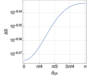
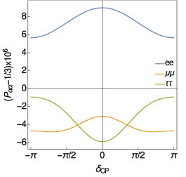
Figure 5: Change in entropy (left) and flavour imbalance (right) after decoherence as a function of CP-violation phase. Initial spectral distortions $\delta$ and $\beta$ are both fixed to the value $10^{-4}$. The values for the mixing angles are given by the global fit of neutrino oscillation data [38] for normal hierarchy.

For non-vanishing CP-violation phase, the difference between probabilities for neutrinos and anti-neutrinos in non-trivial. In the case of the transition from electron to muon neutrinos it is given by

$$P_{e\mu}-P_{\bar{e}\bar{\mu}} = \sin(2\theta_{12})\sin(2\theta_{23})\cos^{2}(\theta_{13})\sin(\theta_{13})\sin(\delta_{\rm CP})$$

$$\times \left[\sin(x_{21})\exp\left({4\int\frac{l_{3}^{2}}{2\mathcal{H}_{3}}dx_{21}}\right)\right.$$ (134)

$$-\sin(x_{31})\exp\left({\int\frac{(l_{3}+\sqrt{3}l_{8})^{2}}{\mathcal{H}_{3}+\sqrt{3}\mathcal{H}_{8}}dx_{31}}\right)$$

$$\left.+\sin(x_{32})\exp\left({\int\frac{(l_{3}-\sqrt{3}l_{8})^{2}}{-\mathcal{H}_{3}+\sqrt{3}\mathcal{H}_{8}}dx_{32}}\right)\right],$$

which is consistent with the literature [45]. In order to stress the role of coherence in this particular result, we use the Gell-Mann coefficients for the solutions contained in equations (96) – (101). We note that differences between neutrinos and anti-neutrinos for any transition probability vanish in the limit of completed decoherence.

We obtain the limit after decoherence is completed of equations (125) – (133) and then rotate to the flavour basis. For simplicity we replace the mixing angles for the best-fit in the global analysis [38] for normal neutrino hierarchy

$$\bar{\rho}_{{\rm f}0} = 1/3,$$ (135)

$$\bar{\rho}_{{\rm f}1} = -\delta[0.05032+0.03192\cos(\delta_{\rm CP})]$$ (136)

$$-\beta[0.00900+0.01447\cos(\delta_{\rm CP})+0.00104\cos(2\delta_{\rm CP})],$$

$$\bar{\rho}_{{\rm f}2} = -0.03192\delta\sin(\delta_{\rm CP})+\beta[0.01276\sin(\delta_{\rm CP})-0.00104\sin(2\delta_{\rm CP})],$$ (137)

$$\bar{\rho}_{{\rm f}3} = \delta[0.08767-0.00626\cos(\delta_{\rm CP})]$$ (138)

$$-\beta[0.02992-0.01053\cos(\delta_{\rm CP})+0.00169\cos(2\delta_{\rm CP})],$$

$$\bar{\rho}_{{\rm f}4} = \delta[0.06333-0.02536\cos(\delta_{\rm CP})]$$ (139)

$$+\beta[0.00920+0.04442\cos(\delta_{\rm CP})-0.00082\cos(2\delta_{\rm CP})],$$

$$\bar{\rho}_{{\rm f}5} = -0.02536\delta\sin(\delta_{\rm CP})$$ (140)

$$-\beta[0.01014\sin(\delta_{\rm CP})+0.00082\sin(2\delta_{\rm CP})],$$

$$\bar{\rho}_{{\rm f}6} = +\delta[0.09423+0.00290\cos(\delta_{\rm CP})]$$ (141)

$$+\beta[0.05407+0.00808\cos(\delta_{\rm CP})-0.00079\cos(2\delta_{\rm CP})]$$

$$\bar{\rho}_{{\rm f}7} = 0.00551\beta\sin(\delta_{\rm CP})+0.01285\delta\sin(\delta_{\rm CP}),$$ (142)

$$\bar{\rho}_{{\rm f}8} = \delta[0.02539+0.01084\cos(\delta_{\rm CP})]$$ (143)

$$+\beta[0.00133+0.01065\cos(\delta_{\rm CP})+0.00293\cos(2\delta_{\rm CP})],$$

which are consistent with the solution for vanishing CP-violation phase present in equations (102) – (110).

Using the averaged solution in mass basis for simplicity, we can calculate the change in the von Neumann entropy using equation (5)

$$\Delta S=\frac{3\delta^{2}}{64}\cos^{2}\theta_{13}\left[9-\cos(4\theta_{12})-(7+\cos(4\theta_{12}))\cos(2\theta_{13})\right]$$

$$+\frac{\beta^{2}}{192}\left[64-\cos^{2}(2\theta_{23})\left(2\cos(4\theta_{12})(\cos(2\theta_{13})-3)^{2}+12\cos(2\theta_{13})+7\cos(4\theta_{13})+37\right)\right]$$

$$-\frac{\beta^{2}}{3}\cos^{2}(\delta_{\rm CP})\sin^{2}(2\theta_{12})\sin^{2}\theta_{13}\sin^{2}(2\theta_{23})$$

$$-\frac{\beta^{2}}{48}\cos(\delta_{\rm CP})\sin(4\theta_{12})[\sin(3\theta_{13})-7\sin\theta_{13}]\sin(4\theta_{23})$$

$$+\frac{\beta\delta}{16}\cos^{2}\theta_{13}\cos(2\theta_{23})\left[5-(\cos(4\theta_{12})+7)\cos(2\theta_{13})+3\cos(4\theta_{12})\right]$$

$$-\frac{\beta\delta}{4}\cos(\delta_{\rm CP})\cos^{2}\theta_{13}\sin(4\theta_{12})\sin\theta_{13}\sin(2\theta_{23})+\mathcal{O}(4)\ .$$ (144)

The change in entropy is also consistent with the case of a vanishing CP-violation phase in equation (124), and identical for vanishing initial difference between muon and tau ($\beta=0$). In figure 5 we show the probability to find a cosmological neutrino in a specified flavour state in the averaged limit as well as the expected change in the entropy, both as functions of the CP-violation phase.

References

- [1] R. H. Cyburt, B. D. Fields, K. A. Olive and E. Skillman, New BBN limits on physics beyond the standard model from , Astropart. Phys. 23 (2005) 313–323, [astro-ph/0408033].
- [2] E. Komatsu, K. M. Smith, J. Dunkley, C. L. Bennett, B. Gold, G. Hinshaw et al., Seven-year Wilkinson Microwave Anisotropy Probe (WMAP) Observations: Cosmological Interpretation, Astrophys.J.Suppl. 192 (Feb., 2011) 18, [1001.4538].
- [3] Planck Collaboration, P. A. R. Ade, N. Aghanim, M. Arnaud, M. Ashdown, J. Aumont et al., Planck 2015 results. XIII. Cosmological parameters, A&A 594 (Sept., 2016) A13, [1502.01589].
- [4] S. Weinberg, Universal Neutrino Degeneracy, Phys. Rev. 128 (Nov, 1962) 1457–1473.
- [5] S. Betts et al., Development of a Relic Neutrino Detection Experiment at PTOLEMY: Princeton Tritium Observatory for Light, Early-universe, Massive-Neutrino Yield, in Proceedings, 2013 Community Summer Study on the Future of U.S. Particle Physics, 2013. 1307.4738.
- [6] A. Dolgov, S. Hansen, S. Pastor, S. Petcov, G. Raffelt and D. Semikoz, Cosmological bounds on neutrino degeneracy improved by flavor oscillations, Nucl.Phys. B 632 (2002) 363 – 382.
- [7] S. Hannestad, Oscillation effects on neutrino decoupling in the early universe, Phys.Rev. D65 (2002) 083006, [astro-ph/0111423].
- [8] M. M. Guzzo, P. C. de Holanda and R. L. N. Oliveira, Quantum Dissipation in a Neutrino System Propagating in Vacuum and in Matter, Nucl. Phys. B908 (2016) 408–422, [1408.0823].
- [9] G. B. Gomes, M. M. Guzzo, P. C. de Holanda and R. L. N. Oliveira, Parameter Limits for Neutrino Oscillation with Decoherence in KamLAND, 1603.04126.
- [10] J. A. B. Coelho, W. A. Mann and S. S. Bashar, Nonmaximal mixing at NOvA from neutrino decoherence, Phys. Rev. Lett. 118 (2017) 221801, [1702.04738].
- [11] G. Lindblad, On the generators of quantum dynamical semigroups, Commun.Math. Phys. 48 (1976) 119.
- [12] D. Notzold and G. Raffelt, Neutrino Dispersion at Finite Temperature and Density, Nucl. Phys. B307 (1988) 924–936.
- [13] B. H. J. McKellar and M. J. Thomson, Oscillating neutrinos in the early Universe, Phys. Rev. D 49 (Mar, 1994) 2710–2728.
- [14] C. Volpe, D. Vaananen and C. Espinoza, Extended evolution equations for neutrino propagation in astrophysical and cosmological environments, Phys. Rev. D87 (2013) 113010, [1302.2374].
- [15] Y. Y. Y. Wong, Analytical treatment of neutrino asymmetry equilibration from flavor oscillations in the early universe, Phys. Rev. D66 (2002) 025015, [hep-ph/0203180].
- [16] A. D. Dolgov, S. H. Hansen, S. Pastor, S. T. Petcov, G. G. Raffelt and D. V. Semikoz, Cosmological bounds on neutrino degeneracy improved by flavor oscillations, Nucl. Phys. B632 (2002) 363–382, [hep-ph/0201287].
- [17] G. Barenboim, W. H. Kinney and W.-I. Park, Flavor versus mass eigenstates in neutrino asymmetries: implications for cosmology, 1609.03200.
- [18] G. Mangano, G. Miele, S. Pastor, T. Pinto, O. Pisanti et al., Relic neutrino decoupling including flavor oscillations, Nucl.Phys. B729 (2005) 221–234, [hep-ph/0506164].
- [19] N. Saviano, A. Mirizzi, O. Pisanti, P. D. Serpico, G. Mangano and G. Miele, Multi-momentum and multi-flavour active-sterile neutrino oscillations in the early universe: role of neutrino asymmetries and effects on nucleosynthesis, Phys. Rev. D87 (2013) 073006, [1302.1200].
- [20] D. Kirilova, Neutrino spectrum distortion due to oscillations and its BBN effect, Int. J. Mod. Phys. D13 (2004) 831–842, [hep-ph/0209104].
- [21] P. Langacker, S. Petcov, G. Steigman and S. Toshev, Implications of the mikheyev-smirnov-wolfenstein (MSW) mechanism of amplification of neutrino oscillations in matter, Nuclear Physics B 282 (1987) 589 – 609.
- [22] S. Donadi, A. Bassi, L. Ferialdi and C. Curceanu, The effect of spontaneous collapses on neutrino oscillations, Found. Phys. 43 (2013) 1066–1089, [1207.5997].
- [23] C. Giunti, Coherence and wave packets in neutrino oscillations, Found. Phys. Lett. 17 (2004) 103–124, [hep-ph/0302026].
- [24] E. K. Akhmedov and A. Yu. Smirnov, Paradoxes of neutrino oscillations, Phys. Atom. Nucl. 72 (2009) 1363–1381, [0905.1903].
- [25] Hannestad, Steen and Raffelt, Georg G. and Sigl, Günter and Wong, Yvonne Y. Y., Self-induced conversion in dense neutrino gases: Pendulum in flavor space, Phys. Rev. D 74 (Nov, 2006) 105010.
- [26] R. Oliveira and M. Guzzo, Dissipation and in neutrino oscillations, The European Physical Journal C 73 (2013) 1–10.
- [27] J. Kersten and A. Yu. Smirnov, Decoherence and oscillations of supernova neutrinos, Eur. Phys. J. C76 (2016) 339, [1512.09068].
- [28] E. Akhmedov, J. Kopp and M. Lindner, Collective neutrino oscillations and neutrino wave packets, 1702.08338.
- [29] D. Pfenniger and V. Muccione, Cosmological Neutrino Entanglement and Quantum Pressure, Astron. Astrophys. 456 (2006) 45, [astro-ph/0605354].
- [30] A. Bernardini, Cosmological neutrino entropy changes due to flavor statistical mixing, Europhys.Lett. 103 (2013) 30005, [1204.1504].
- [31] S. L. Adler, Comment on a proposed Super-Kamiokande test for quantum gravity induced decoherence effects, Phys. Rev. D62 (2000) 117901, [hep-ph/0005220].
- [32] T. Ohlsson, Equivalence between neutrino oscillations and neutrino decoherence, Phys. Lett. B502 (2001) 159–166, [hep-ph/0012272].
- [33] P. Pearle, Simple derivation of the Lindblad equation, European Journal of Physics 33 (July, 2012) 805–822, [1204.2016].
- [34] S. Weinberg, Lindblad Decoherence in Atomic Clocks, Phys. Rev. A94 (2016) 042117, [1610.02537].
- [35] J. Distler and S. Paban, von Neumann’s Formula, Measurements and the Lindblad Equation, 1702.01724.
- [36] G. Barenboim, N. E. Mavromatos, S. Sarkar and A. Waldron-Lauda, Quantum decoherence and neutrino data, Nucl. Phys. B758 (2006) 90–111, [hep-ph/0603028].
- [37] Particle Data Group collaboration, K. A. Olive et al., Review of Particle Physics, Chin. Phys. C38 (2014) 090001.
- [38] D. Forero, M. Tortola and J. Valle, Global status of neutrino oscillation parameters after Neutrino-2012, Phys.Rev. D86 (2012) 073012, [1205.4018].
- [39] F. Capozzi, E. Di Valentino, E. Lisi, A. Marrone, A. Melchiorri and A. Palazzo, Phys. Rev. D 95, no. 9, 096014 (2017) [hep-ph/1703.04471] .
- [40] G. Arfken, H. Weber and F. Harris, Mathematical Methods for Physicists, Sixth Edition. Elsevier/Academic Press, 2005.
- [41] G. Mangano, G. Miele, S. Pastor and M. Peloso, A Precision calculation of the effective number of cosmological neutrinos, Phys. Lett. B534 (2002) 8–16, [astro-ph/0111408].
- [42] S. Hannestad and J. Brandbyge, The Cosmic Neutrino Background Anisotropy - Linear Theory, JCAP 1003 (2010) 020, [0910.4578].
- [43] S. Weinberg, Entropy generation and the survival of protogalaxies in an expanding universe, Astrophys.J. 168 (1971) 175.
- [44] N. Straumann, On Radiative Fluids, Helv. Phys. Acta 49 (1976) 269.
- [45] V. Barger, K. Whisnant and R. J. N. Phillips, CP Nonconservation in Three-Neutrino Oscillations, Phys. Rev. Lett. 45 (Dec, 1980) 2084–2088.