Non-linear Frequency Transduction of Nano-mechanical Brownian Motion
Olivier Maillet1, Xin Zhou1, Rasul Gazizulin1, Ana Maldonado Cid1, Martial Defoort1,2, Olivier Bourgeois1 & Eddy Collin1,∗

1Université Grenoble Alpes, Institut Néel - CNRS, F-38042 Grenoble, France
2Now at: CEA, LETI, MINATEC Campus, 17 rue des Martyrs, 38054 Grenoble Cedex 9, France
*: Corresponding Author

We report on experiments addressing the non-linear interaction between a nano-mechanical mode and position fluctuations. The Duffing non-linearity transduces the Brownian motion of the mode, and of other non-linearly coupled ones, into frequency noise. This mechanism, ubiquitous to all weakly-nonlinear resonators thermalized to a bath, results in a phase diffusion process altering the motion: two limit behaviors appear, analogous to motional narrowing and inhomogeneous broadening in NMR. Their crossover is found to depend non-trivially on the ratio of the frequency noise correlation time to its magnitude. Our measurements obtained over an unprecedented range covering the two limits match the theory of Y. Zhang and M. I. Dykman, Phys. Rev. B 92, 165419 (2015), with no free parameters. We finally discuss the fundamental bound on frequency resolution set by this mechanism, which is not marginal for bottom-up nanostructures.

1 Introduction

Emerging from the tremendous development of micro/nano technologies, nano-electro-mechanical systems (NEMS) have opened unique capabilities to both engineers and physicists. In the first place, they serve as ultra-sensitive probes for force sensing [2] with applications e.g. to mass, charge, and even single electronic spin detection [3, 4, 5]. In the second place, these objects are extremely fruitful (weakly) non-linear devices that are able to implement useful functions like e.g. mechanical frequency mixing [6], amplification [7] and bit storage [8]. On the fundamental level, high-quality NEMS structures can be thought of as model systems in which basic phenomena can be advantageously reproduced; one example being the ubiquitous bifurcation mechanism [9, 10, 11].

Ultimately, when coupled to a quantum-limited detection scheme such as a microwave cavity or a Single-Electron Transistor, their sensitivity can be brought to the quantum limit [12, 13]. This leads to a unique platform realizing the “ultimate force detector” foreseen by C. Caves in the 80’s [14]. Such moving structures that are macroscopic relative to the atomic scale but follow the laws of quantum mechanics are currently under development for tests of quantum foundations [15, 16, 17]. Furthermore, they are thought to be a unique new quantum electronics component enabling e.g. coherent photon conversion from the microwave to the optical domain [18, 19].

Essentially all applications require in the first place the resonance frequency of the mechanical mode in use to be as stable as possible. As such, the understanding of the sources of frequency fluctuations in nano-mechanical devices becomes an essential technical topic [24, 2, 21, 22, 20, 23]. But in the first place, it is also a fundamental research goal: the measured frequency noise in actual devices is much larger than all expectations [23, 25, 26, 27], demonstrating even non-linear features for carbon-based systems [28, 29]. Thus, attempts have been made to model noise sources [30, 31], or to create model experiments experimentally demonstrating the underlying mechanisms [20, 34, 32, 35].

Clever driving schemes taking advantage of non-linearities have been devised to significantly suppress frequency noise [36, 37]. But what shall be an “ideally frequency-noise minimizing” nano-mechanical system in the first place? We know that at lowest order, the dynamics of a mechanical structure can be described by a family of normal modes which are nothing but independent harmonic oscillators. Pushing to the next order, these modes are weakly non-linear (so-called Duffing resonators) and are dispersively coupled one to the other [38, 39, 40]. Since all of the modes are unavoidably coupled to a thermal reservoir (ideally the same one), Brownian motion of each of the modes will transduce into a frequency noise on all the others [20, 35, 23, 41, 30], and also on itself. Even in a system realized with ideal materials having no internal sources of noise, this built-in mechanism shall fix an ultimate limit to the mechanical resonance frequencies stability at T0𝑇0T\neq 0. Only in the limit of T0𝑇0T\rightarrow 0, when all the modes are in their quantum ground state, do the dispersive couplings lead to a simple frequency renormalization of the resonances through the zero-point-fluctuations of each of them: a sort of mechanical Lamb shift that dresses all the modes [42].

In the present article, we report on a model experiment in which we use very high quality silicon-nitride NEMS cooled down to Kelvin temperatures. A single mode is driven by a stochastic force, leading to effective temperatures as high as 109superscript10910^{9}\leavevmode\nobreak\ K for this mode only. We extract the effect of this “artificial out-of-equilibrium heating” on the mode itself, both by measuring the spectrum of the motion and by measuring the simultaneous response of the same mode to a sine-wave excitation. The effect on a nearby mode is measured with the sine-wave excitation scheme. The setup is carefully calibrated [43], while the devices’ characteristics are obtained by both measurements and calculations; the agreement with theory is obtained with no free parameters. Besides, the experiment is performed on different devices proving the reproducibility of the results.

We demonstrate experimentally the two regimes of the Brownian motion transduction, named after analog phenomena present in Nuclear Magnetic Resonance (NMR): “motional narrowing” and “inhomogeneous broadening” [32]. Based on Ref. [41] and simple expansions of Euler-Bernoulli theory (including non-linear coefficients [39, 40, 49]) we give the analytic tools enabling the calculation of the “ultimate frequency stability” reached by any doubly-clamped device, depending on stress, dimensions and temperature T𝑇T [46]. For bottom-up structures like e.g. carbon nanotubes with high aspect ratio, this limit is not marginal [30].

2 Results

2.1 The nano-electro-mechanical systems
Refer to caption
Refer to caption
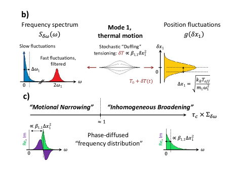
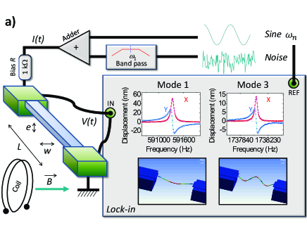
Figure 1: (Color online). a) The nano-mechanical beams (left) are driven by means of a d.c. magnetic field B𝐵B and an a.c. current consisting of the sum of two components (top): a sine-wave which frequency is swept around a chosen mode (n=1𝑛1n=1 or n=3𝑛3n=3 here) and a Gaussian white noise filtered around mode n=1𝑛1n=1. The motion is detected with a lock-in amplifier through the induced voltage V𝑉V, leading to the two quadratures X𝑋X and Y𝑌Y for each mode n=1𝑛1n=1 or n=3𝑛3n=3 (right; lines are Lorentz fits and images Ansys®  numerical simulations). Data corresponding to beam 300μ𝜇\leavevmode\nobreak\ \mum-n1 in the linear regime. b) The Gaussian noise force applied onto the mode (here mode 1, center) is equivalent to an effective temperature Teffsubscript𝑇𝑒𝑓𝑓T_{ef\!f} (right). The motion transduces into a frequency noise (spectrum on the left) because of the Duffing non-linearity β1,1subscript𝛽11\beta_{1,1} due to tensioning. Only the low frequency part of these fluctuations is relevant (in blue, with the d.c. average marked by an arrow), the high frequency term (red) is filtered-out by the dynamics of the mode (adiabatic picture in the rotating frame of the motion). c) Depending on the amplitude of frequency fluctuations ΣδωsubscriptΣ𝛿𝜔\Sigma_{\delta\omega} (their standard deviation [Sδω𝑑ω]1/2proportional-toabsentsuperscriptdelimited-[]subscript𝑆𝛿𝜔differential-d𝜔12\propto[\int\!S_{\delta\omega}d\omega]^{1/2}) with respect to their correlation time τcsubscript𝜏𝑐\tau_{c} (here 1/Δω11Δsubscript𝜔11/\Delta\omega_{1}, with Δω1Δsubscript𝜔1\Delta\omega_{1} the linewidth of the noisy mode) two regimes are distinguished: “motional narrowing” and “inhomogeneous broadening”. This is due to the underlying dynamics of phase diffusion experienced by the mechanical mode, leading to the averaged “frequency distribution” depicted below the horizontal arrow (green and violet).

The devices under study are doubly-clamped silicon-nitride nano-beams having width w=𝑤absentw=300  nm and thickness eSiN=subscript𝑒𝑆𝑖𝑁absente_{SiN}=100  nm. Two high-stress (1  GPa) beams of L=𝐿absentL=300μ𝜇\leavevmode\nobreak\ \mum length have been measured plus a 250μ𝜇\leavevmode\nobreak\ \mum one (samples 300μ𝜇\leavevmode\nobreak\ \mum-n1, 300μ𝜇\leavevmode\nobreak\ \mum-n2 and 250μ𝜇\leavevmode\nobreak\ \mum-n1), together with one low-stress (100  MPa) L=𝐿absentL=15μ𝜇\leavevmode\nobreak\ \mum shorter beam (15μ𝜇\leavevmode\nobreak\ \mum-n1). A thin layer of aluminum (eMsubscript𝑒𝑀e_{M} about 30  nm to 90  nm thick) has been added on top to create electrical contacts. The experiments are performed at 4.2  K in cryogenic vacuum (pressure <106m\bbarabsentsuperscript106m\bbar<10^{-6}\leavevmode\nobreak\ \mathrm{m}\bbar).

Fig. 1 a) shows a schematic of the setup. For each device and each mode n𝑛n (or m𝑚m) studied, we perform a careful calibration based on the technique developed in Ref. [43]. We can thus infer forces Fnsubscript𝐹𝑛F_{n} and displacements xnsubscript𝑥𝑛x_{n} in S.I. units, and compute the devices characteristics (namely mass mnsubscript𝑚𝑛m_{n}, spring constant knsubscript𝑘𝑛k_{n}, non-linear coefficients βn,msubscript𝛽𝑛𝑚\beta_{n,m}). These match the expected calculated values; note that a particular care has been taken in the calibration of the noise source. The only fit parameter is indeed an overall correction of the force noise not exceeding 15  % in amplitude (same order as in Ref. [11]). Actuation and detection are performed with the magnetomotive scheme [43, 47]. A drive current (composed of both the Gaussian noise component centered around resonance frequency ω1subscript𝜔1\omega_{1} and a sine-wave of frequency ω𝜔\omega close to ωnsubscript𝜔𝑛\omega_{n}, with n=1𝑛1n=1 or n=3𝑛3n=3) is injected in the NEMS metallic layer through a home-made adder and a 1k1k1\leavevmode\nobreak\ \mathrm{k}\mathrm{\SIUnitSymbolOhm} bias resistor. In an in-plane d.c. magnetic field orthogonal to the beams, this generates an out-of-plane driving force Fn(t)subscript𝐹𝑛𝑡F_{n}(t) with harmonic component Fn0cos(ωt)superscriptsubscript𝐹𝑛0𝜔𝑡F_{n}^{0}\cos(\omega t). The motion is detected through the induced voltage by means of a standard lock-in detection. We obtain the two quadratures, in-phase (X) and out-of-phase (Y) with respect to the local oscillator.

In order to preserve our calibration capabilities, the lock-in has also been used for the spectral measurements SXn(ω)subscriptsuperscript𝑆𝑛𝑋𝜔S^{n}_{X}(\omega) of the Brownian motion of mode n=1𝑛1n=1. Moreover, this enables to measure fluctuations on each of the two quadratures X𝑋X, Y𝑌Y independently (plus their cross-correlations). When the sinusoidal excitation is weak (or nonexistent), the spectra on X and Y are equivalent and no correlations are detected; this is the range of validity of the work presented here. However, signatures of squeezed statistics of motion [44] can be observed on measured spectra when the sinusoidal excitation is too large. Details on the measurement technique, calibrations and calculated parameters can be found in S.M. [46].

2.2 Dispersive coupling driven by stochastic motion

Linear motion of thin nano-beams is very well described by the Euler-Bernoulli equation [48]. The basic ingredients involved are the inertia (through the density ρbeamsubscript𝜌𝑏𝑒𝑎𝑚\rho_{beam}), the Young’s modulus Ebeamsubscript𝐸𝑏𝑒𝑎𝑚E_{beam} and the tension T0subscript𝑇0T_{0} generated by the in-built stress. For doubly-clamped beams, the non-linear behaviour is well understood: it arises from the stretching of the device under transverse motion x𝑥x [40, 39, 49]. This geometric non-linearity results in a tensioning T0+δTsubscript𝑇0𝛿𝑇T_{0}+\delta T of the beam with δTx2proportional-to𝛿𝑇superscript𝑥2\delta T\propto x^{2}, which can be incorporated into the beam equation [49]. This leads to a frequency shift of the modes that is proportional to the square of the displacement. When only two modes n,m𝑛𝑚n,m are under study, it writes:

ωnsubscript𝜔𝑛\displaystyle\omega_{n} =\displaystyle= ωn0+βn,nxn2+βn,mxm2,superscriptsubscript𝜔𝑛0subscript𝛽𝑛𝑛superscriptsubscript𝑥𝑛2subscript𝛽𝑛𝑚superscriptsubscript𝑥𝑚2\displaystyle\omega_{n}^{0}+\beta_{n,n}x_{n}^{2}+\beta_{n,m}x_{m}^{2}, (1)
ωmsubscript𝜔𝑚\displaystyle\omega_{m} =\displaystyle= ωm0+βm,mxm2+βm,nxn2,superscriptsubscript𝜔𝑚0subscript𝛽𝑚𝑚superscriptsubscript𝑥𝑚2subscript𝛽𝑚𝑛superscriptsubscript𝑥𝑛2\displaystyle\omega_{m}^{0}+\beta_{m,m}x_{m}^{2}+\beta_{m,n}x_{n}^{2}, (2)

where we introduced ωn0superscriptsubscript𝜔𝑛0\omega_{n}^{0}, ωm0superscriptsubscript𝜔𝑚0\omega_{m}^{0} the linear resonance frequencies, and the Duffing non-linear coefficients βi,jsubscript𝛽𝑖𝑗\beta_{i,j} [40]. We remind for the interested reader the mathematical derivation of these expressions in S.M. [46].

Eqs. (1-2) can be adapted when one of the motions, say xnsubscript𝑥𝑛x_{n}, is a stochastic variable: xn=xn0+δxnsubscript𝑥𝑛superscriptsubscript𝑥𝑛0𝛿subscript𝑥𝑛x_{n}=x_{n}^{0}+\delta x_{n}, with xn0superscriptsubscript𝑥𝑛0x_{n}^{0} the certain component and δxn𝛿subscript𝑥𝑛\delta x_{n} the Gaussian and centered random component. In order to introduce the phenomenon, let us first consider the case depicted in Fig. 1 b), where only one mode n𝑛n is addressed. We apply on n=1𝑛1n=1 a Gaussian random force δFn(t)𝛿subscript𝐹𝑛𝑡\delta F_{n}(t) of spectrum SFn(ω)subscriptsuperscript𝑆𝑛𝐹𝜔S^{n}_{F}(\omega) whose strength can be converted into an effective temperature Teffsubscript𝑇𝑒𝑓𝑓T_{ef\!f} through the Fluctuation-Dissipation Theorem SFn=2kBTeffmnΔωnsubscriptsuperscript𝑆𝑛𝐹2subscript𝑘𝐵subscript𝑇𝑒𝑓𝑓subscript𝑚𝑛Δsubscript𝜔𝑛S^{n}_{F}=2k_{B}T_{ef\!f}m_{n}\Delta\omega_{n}. ΔωnΔsubscript𝜔𝑛\Delta\omega_{n} is the linewidth of the resonance of mode n𝑛n (with Qn=ωn0/Δωnsubscript𝑄𝑛superscriptsubscript𝜔𝑛0Δsubscript𝜔𝑛Q_{n}=\omega_{n}^{0}/\Delta\omega_{n} the quality factor), and SFn(ω)subscriptsuperscript𝑆𝑛𝐹𝜔S^{n}_{F}(\omega) is white around the mode studied only (and negligible elsewhere). The mechanical mode thus experiences position fluctuations (Brownian motion) linked to SFnsubscriptsuperscript𝑆𝑛𝐹S^{n}_{F} through the mechanical susceptibility, whose spectrum SXn(ω)superscriptsubscript𝑆𝑋𝑛𝜔S_{X}^{n}(\omega) is peaked around ωn0superscriptsubscript𝜔𝑛0\omega_{n}^{0}. Since Teff4.2much-greater-thansubscript𝑇𝑒𝑓𝑓4.2T_{ef\!f}\gg 4.2\leavevmode\nobreak\ K the experimental temperature, we safely neglect all other sources of fluctuations while enabling a thorough tuning of the Brownian motion amplitude of mode n𝑛n only.

Refer to caption
Refer to caption
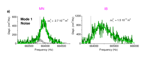
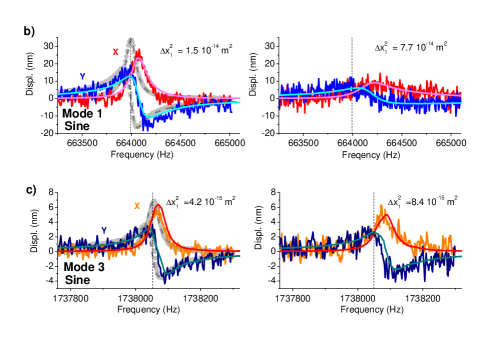
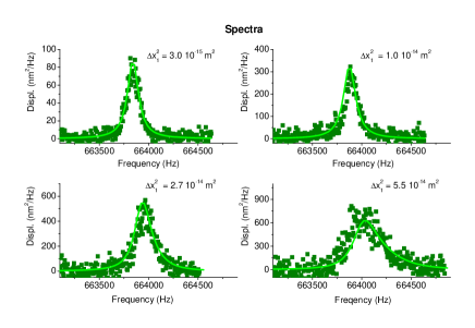
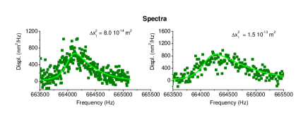
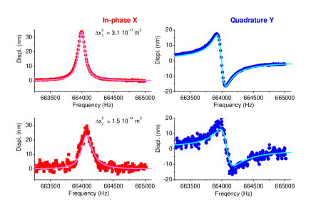
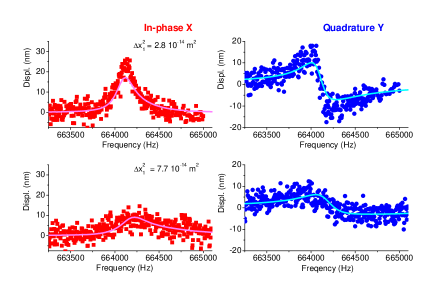
Figure 2: (Color online). (a) Brownian motion spectra measured on mode n=1𝑛1n=1 of sample 300μ𝜇\leavevmode\nobreak\ \mum-n2 (Duffing spectra). (b) In-phase (X) and quadrature (Y) components measured for mode n=1𝑛1n=1 while driving noise on the same n=1𝑛1n=1 mode for sample 300μ𝜇\leavevmode\nobreak\ \mum-n2 (intra-mode). (c) Same measurement performed on mode n=3𝑛3n=3 while driving fluctuations on n=1𝑛1n=1 for sample 300μ𝜇\leavevmode\nobreak\ \mum-n1 (inter-mode coupling). The standard deviation Δx12Δsuperscriptsubscript𝑥12\Delta x_{1}^{2} (i.e Brownian motion level) is increased from left to right (essentially from MN to IB regime, see Fig. 3), and sinusoidal drives are kept in the linear regime. The grey data are the references obtained for very weak noise levels. The verticals are resonance position without Brownian transduction, and lines theoretical calculations (see text).

2.3 Transduction mechanism

From the Duffing equations, the random motion δxn𝛿subscript𝑥𝑛\delta x_{n} is transduced into a frequency noise Sδω(ω)subscript𝑆𝛿𝜔𝜔S_{\delta\omega}(\omega). Since this dependence is quadratic, the frequency noise is neither Gaussian nor centered. Its spectrum depicted in Fig. 1 b) consists in a low frequency part and a high frequency component peaked around 2ωn2subscript𝜔𝑛2\omega_{n}. The high-frequency fluctuations are essentially filtered out by the mode dynamics, as can be seen in a Rotating Wave Approximation (RWA). Thus, driving the mode with a sine wave force Fn0cos(ωt)superscriptsubscript𝐹𝑛0𝜔𝑡F_{n}^{0}\cos(\omega t) weak enough to remain in the linear response limit, the motion xn0superscriptsubscript𝑥𝑛0x_{n}^{0} will adiabatically follow the slow frequency fluctuations experiencing both a frequency shift and a spectral broadening [41]. The measurement scheme itself is always slow enough to ensure that all fluctuations are spanned while acquiring data. Note that the Brownian fluctuations do not need to be small for the theory to apply.

The phenomenon is non-trivial, and depends strongly on the correlation time of the fluctuations τc=1/Δωnsubscript𝜏𝑐1Δsubscript𝜔𝑛\tau_{c}=1/\Delta\omega_{n}. Defining Σδω=4βn,nΔxn2subscriptΣ𝛿𝜔4subscript𝛽𝑛𝑛Δsuperscriptsubscript𝑥𝑛2\Sigma_{\delta\omega}=4\beta_{n,n}\Delta x_{n}^{2} a frequency noise amplitude parameter (essentially their standard deviation [Sδω𝑑ω]1/2proportional-toabsentsuperscriptdelimited-[]subscript𝑆𝛿𝜔differential-d𝜔12\propto[\int\!S_{\delta\omega}d\omega]^{1/2}), two regimes should be distinguished depending on the magnitude of the product τc×Σδωsubscript𝜏𝑐subscriptΣ𝛿𝜔\tau_{c}\times\Sigma_{\delta\omega}, see Fig. 1 c). The process can be understood in terms of phase-diffusion for the mode studied, the dynamics being averaged over all realizations of the fluctuating resonance frequency δω𝛿𝜔\delta\omega, namely xn0(t)ei0tδω(t′′)dt′′proportional-tosuperscriptsubscript𝑥𝑛0𝑡delimited-⟨⟩superscript𝑒𝑖superscriptsubscript0𝑡𝛿𝜔superscript𝑡′′differential-dsuperscript𝑡′′x_{n}^{0}(t)\propto\left\langle e^{\displaystyle i\int_{0}^{t}\delta\omega(t^{\prime\prime})\mathrm{d}t^{\prime\prime}}\right\rangle [41]. The frequency-domain data can thus be described by a convolution of the linear response by a complex valued distribution of frequencies, as seen from the NEMS (bottom of Fig. 1 c):

FT[exp(+Γnt)cosh(ant)+Γnan(1+2iαn)sinh(ant)](ω),FTdelimited-[]subscriptΓ𝑛𝑡subscript𝑎𝑛𝑡subscriptΓ𝑛subscript𝑎𝑛12𝑖subscript𝛼𝑛subscript𝑎𝑛𝑡𝜔\mathrm{FT}\left[\frac{\exp(+\Gamma_{n}t)}{\cosh(a_{n}t)+\frac{\Gamma_{n}}{a_{n}}\left(1+2i\alpha_{n}\right)\sinh(a_{n}t)}\right]\left(\omega\right), (3)

FT meaning Fourier Transform, with Γn=Δωn/2subscriptΓ𝑛Δsubscript𝜔𝑛2\Gamma_{n}=\Delta\omega_{n}/2 the mode’s relaxation rate, an=Γn1+4iαnsubscript𝑎𝑛subscriptΓ𝑛14𝑖subscript𝛼𝑛a_{n}=\Gamma_{n}\sqrt{1+4i\alpha_{n}} and αn=Σδω2Γn=τc×Σδωsubscript𝛼𝑛subscriptΣ𝛿𝜔2subscriptΓ𝑛subscript𝜏𝑐subscriptΣ𝛿𝜔\alpha_{n}=\frac{\Sigma_{\delta\omega}}{2\Gamma_{n}}=\tau_{c}\times\Sigma_{\delta\omega} the motional narrowing parameter.

By analogy with Nuclear Magnetic Resonance, when τc×Σδω1much-less-thansubscript𝜏𝑐subscriptΣ𝛿𝜔1\tau_{c}\times\Sigma_{\delta\omega}\ll 1 the certain component’s dynamics is said to be in the “motional narrowing” limit (MN), while for τc×Σδω1much-greater-thansubscript𝜏𝑐subscriptΣ𝛿𝜔1\tau_{c}\times\Sigma_{\delta\omega}\gg 1 it lies in the “inhomogeneous broadening” limit (IB). In the former case, the fluctuations are too fast to enable the resolution of the small frequency changes ΣδωsubscriptΣ𝛿𝜔\Sigma_{\delta\omega} [32, 33]: the random variable’s dynamics looses memory too quickly, and only a fraction of the frequency fluctuations impacts the driven motion. This leads to a certain frequency shift which is nothing but the average of the frequency fluctuations proportional to Δxn2Δsuperscriptsubscript𝑥𝑛2\Delta x_{n}^{2}, together with a (weaker, second order) symmetric broadening quadratic in Δxn2Δsuperscriptsubscript𝑥𝑛2\Delta x_{n}^{2} (bottom-left “distribution” in Fig. 1 c). In the latter case, the fluctuations are slow enough so that the full range of frequency fluctuations can be explored by the xn0superscriptsubscript𝑥𝑛0x_{n}^{0} sine-wave response [50, 34]: there is a large asymmetric broadening, which reflects the actual distribution of frequency fluctuations (bottom-right in Fig. 1 c). When mode m=3𝑚3m=3 is sine-wave driven and detected while force noise is still applied onto mode n=1𝑛1n=1, the treatment is identical with the replacement Σδω=2βm,nΔxn2subscriptΣ𝛿𝜔2subscript𝛽𝑚𝑛Δsuperscriptsubscript𝑥𝑛2\Sigma_{\delta\omega}=2\beta_{m,n}\Delta x_{n}^{2} [41]. Besides, an equation similar to Eq. (3) holds for the direct calculation of non-linear Brownian spectra [41]. A brief description of the theoretical tools developed in Ref. [41] is given in S.M. [46].

In the next Section, we present the experimental data and the theoretical calculations corresponding to these two situations. The displacement noise spectrum of mode n=1𝑛1n=1 is also directly measured. We reach the limit where this spectrum itself is imprinted by the Duffing non-linearity [20], and match it to the theory [41]. Since Brownian motions of two mn𝑚𝑛m\neq n distinct modes are not correlated, from these elementary measurements one can then deduce the generic situation where N𝑁N thermalized modes of the same structure are coupled together.
Refer to caption
Refer to caption
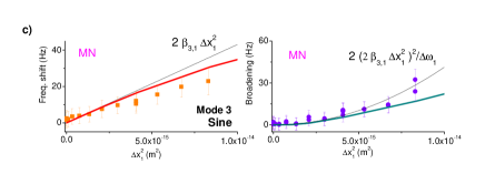
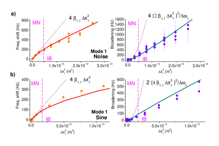
Figure 3: (Color online). Frequency shift (left) and broadening (from FWHH, right) for (a) the (Duffing) spectra measured on mode n=1𝑛1n=1 for sample 300μ𝜇\leavevmode\nobreak\ \mum-n2, (b) the sine-wave excitation of mode n=1𝑛1n=1, with Brownian motion on the same mode n=1𝑛1n=1 for sample 300μ𝜇\leavevmode\nobreak\ \mum-n2 (intra-mode case), and (c) similar result for sine-wave excitation of mode m=3𝑚3m=3, with Brownian motion of mode n=1𝑛1n=1 for sample 300μ𝜇\leavevmode\nobreak\ \mum-n1 (inter-mode). The thin lines are the “motional narrowing” (MN) analytic expansions, with the dashed verticals corresponding to the cross-over towards “inhomogeneous broadening” (IB) when τc×Σδω=1subscript𝜏𝑐subscriptΣ𝛿𝜔1\tau_{c}\times\Sigma_{\delta\omega}=1. The full lines are from the complete theoretical model (see text).

2.4 Measured resonance properties

In Fig. 15 a) we present the direct measurement of the Brownian noise spectra SXn(ω)superscriptsubscript𝑆𝑋𝑛𝜔S_{X}^{n}(\omega) on mode n=1𝑛1n=1 for sample 300μ𝜇\leavevmode\nobreak\ \mum-n2. No sine-wave excitation is applied, neither on n=1𝑛1n=1 nor on m=3𝑚3m=3 modes. The noise level is quoted in terms of standard deviation Δx12Δsuperscriptsubscript𝑥12\Delta x_{1}^{2} instead of Teffsubscript𝑇𝑒𝑓𝑓T_{ef\!f} (or force noise intensity) since this is the physical parameter of importance. For small Brownian excitations, the peak remains Lorentzian. However, when the amplitude of motion becomes large, the non-linear term β1,1subscript𝛽11\beta_{1,1} starts to impact the lineshape: the peak broadens and becomes asymmetric [20, 35]. As expected, the resonance peak globally shifts towards higher frequencies (see Fig. 3 a) for a summary of the spectrum characteristics). The lines are the exact theory from Ref. [41], computed with no free parameters: we call them “Duffing spectra” [46]. Note that no deviations from standard Gaussian statistics are measured in these conditions, as it should be for high-Q𝑄Q devices [45]: spectra on the X quadratures are equivalent to the ones measured on Y, and no cross-correlations are detected [46].

We turn next to the case of the intra-mode coupling. We still drive mode n=1𝑛1n=1 with white noise, but we also measure and drive it with a sine-wave signal. Mode m=3𝑚3m=3 is left unexcited. Data and theory from Ref. [41] are compared in Fig. 15 b) with no free parameters. The X lineshapes look like the peaks obtained in the “Duffing spectrum” case, Fig. 15. The effect of the added force noise on the mode is again twofold: first, the resonance peak slightly shifts towards higher frequencies, and second it broadens (consequently flattens) and acquires an asymmetric shape. In Fig. 3 b) we summarize the characteristics of the measured resonance lines on device 300μ𝜇\leavevmode\nobreak\ \mum-n2 (obtained from the X quadrature).

Measured resonance lines and calculations in the inter-mode case (sine-wave driving and measuring mode m=3𝑚3m=3 while adding force noise on mode n=1𝑛1n=1) are shown in Fig. 15 c). They resemble very much the intra-mode results of Fig. 15, even though the quality of the data did not enable to reach as high fluctuation levels (see Fig. 3 c). More data can be found in S.M. [46].

The three basic situations are compared in Fig. 3: we show the characteristics of the measured spectra and resonance lines on 300μ𝜇\leavevmode\nobreak\ \mum devices in terms of frequency shift (position of the maximum of the resonance peak) and broadening (measured from the Full Width at Half Height, FWHH). The same characteristics for 250μ𝜇\leavevmode\nobreak\ \mum and 15μ𝜇\leavevmode\nobreak\ \mum devices are also shown in S.M. [46]: since the non-linear coefficients depend strongly on the length L𝐿L of the structures, this demonstrates the robustness of the effect.
Refer to caption
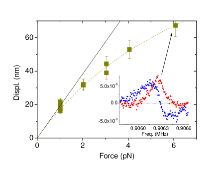
Figure 4: Large sine-wave excitation forces (Color online). Amplitude of the sine-wave response peak as a function of excitation force for mode n=1𝑛1n=1 of device 250μ𝜇\leavevmode\nobreak\ \mum-n1. Force noise is applied on the same mode n=1𝑛1n=1 such that Δx12=2.2 1015Δsuperscriptsubscript𝑥12superscript2.21015\Delta x_{1}^{2}=2.2\,10^{-15}\leavevmode\nobreak\ m2. The full line is the linear theory, which clearly does not fit the data (squares and dashed guide). The inset corresponds to the largest drive measured peak.

The global agreement between data and theory is remarkable. Essentially, “Duffing spectra”, intra-mode and inter-mode Brownian frequency transduction display the same characteristic features. This highlights that the main ingredient is the dynamics of the noisy mode, not the one of the chosen probe. From Fig. 3, we see that we span the whole range of the phenomenon from “motional narrowing” to “inhomogeneous broadening”. In the “motional narrowing” limit, indeed the first order effect is a global frequency shift proportional to Δxn2Δsuperscriptsubscript𝑥𝑛2\Delta x_{n}^{2}. On the other hand, in the “inhomogeneous broadening” range the main feature is the asymmetric broadening which is nothing but the image of the frequency distribution (inhomogeneity in time-domain, as opposed to position-domain for NMR [34]). Further technical discussions of these two limits can be found in S.M. [46].

However, the theory of Ref. [41] applies for sinusoidal excitation strengths lying within the linear response range. When the motion amplitude is increased beyond this limit, new phenomena are expected to take place like e.g. the parametric squeezing of the Brownian motion [44]. One signature obtained experimentally that fails to be reproduced by the theory is shown in Fig. 4: for large sine-wave excitations, the amplitude of the detected mechanical peak lies below the calculation, as if the impact of frequency noise was stronger than expected. In S.M. [46], we show that the noise spectra measured on mode n𝑛n are indeed altered by the back-action of the sine-wave response xn0superscriptsubscript𝑥𝑛0x_{n}^{0}; the X𝑋X and Y𝑌Y quadratures are not equivalent anymore, and cross-correlations are non-zero at some peculiar frequencies. Further work both theoretical and experimental is required to explore this new dynamical range.

2.5 Application to a thermalized family of modes

For a physical thermal bath, the device is always in the “motional narrowing” limit. In this case, the linear response of mode n𝑛n to a weak sinusoidal drive remains Lorentzian, with a resonance frequency “dressed” by the Brownian motion of all modes (global frequency shift proportional to T𝑇T). This is essentially analogous to a mechanical Lamb shift [42], in the classical domain. Furthermore the linewidth of the resonance is impacted by a T2superscript𝑇2T^{2} term, a “thermal decoherence” effect.

Reproducing results from Ref. [41], these can be written at lowest order in terms of simple expansions, respectively for mode n𝑛n:

ωnsubscript𝜔𝑛\displaystyle\omega_{n} =\displaystyle= ωn0+4βn,nΔxn2superscriptsubscript𝜔𝑛04subscript𝛽𝑛𝑛Δsuperscriptsubscript𝑥𝑛2\displaystyle\omega_{n}^{0}+4\beta_{n,n}\Delta x_{n}^{2} (4)
+\displaystyle+ mn2βn,mΔxm2+m2barβn,mΔym2,subscript𝑚𝑛2subscript𝛽𝑛𝑚Δsuperscriptsubscript𝑥𝑚2subscriptsuperscript𝑚2barsubscript𝛽𝑛superscript𝑚Δsuperscriptsubscript𝑦superscript𝑚2\displaystyle\sum_{m\neq n}2\beta_{n,m}\Delta x_{m}^{2}+\sum_{m^{\prime}}2\mathrm{bar}{\beta}_{n,m^{\prime}}\Delta y_{m^{\prime}}^{2},
ΔωnΔsubscript𝜔𝑛\displaystyle\Delta\omega_{n} =\displaystyle= Δωn0+2(4βn,nΔxn2)2Δωn0Δsuperscriptsubscript𝜔𝑛02superscript4subscript𝛽𝑛𝑛Δsuperscriptsubscript𝑥𝑛22Δsuperscriptsubscript𝜔𝑛0\displaystyle\Delta\omega_{n}^{0}+2\frac{\left(4\beta_{n,n}\Delta x_{n}^{2}\right)^{2}}{\Delta\omega_{n}^{0}} (5)
+\displaystyle\!\!\!\!\!\!\!\!\!\!\!\!\!\!\!\!\!\!\!+ mn2(2βn,mΔxm2)2Δωm0+m2(2barβn,mΔym2)2Δbarωm0.subscript𝑚𝑛2superscript2subscript𝛽𝑛𝑚Δsuperscriptsubscript𝑥𝑚22Δsuperscriptsubscript𝜔𝑚0subscriptsuperscript𝑚2superscript2barsubscript𝛽𝑛superscript𝑚Δsuperscriptsubscript𝑦superscript𝑚22Δbarsuperscriptsubscript𝜔superscript𝑚0\displaystyle\!\!\!\!\!\!\!\!\!\!\!\!\!\!\sum_{m\neq n}2\frac{\left(2\beta_{n,m}\Delta x_{m}^{2}\right)^{2}}{\Delta\omega_{m}^{0}}+\sum_{m^{\prime}}2\frac{\left(2\mathrm{bar}{\beta}_{n,m^{\prime}}\Delta y_{m^{\prime}}^{2}\right)^{2}}{\Delta\mathrm{bar}{\omega}_{m^{\prime}}^{0}}.

The validity of these expansions has been experimentally verified in the present work for two modes only, Fig. 3. They can be extended in this simple way to many modes since the Brownian motion between nm𝑛𝑚n\neq m is uncorrelated. For the sake of completeness, we also added the sum over the other family of transverse modes (in y𝑦\vec{y} direction), which coefficients are designed with a bar, and the index with a prime (the position standard deviation simply writes Δym2Δsuperscriptsubscript𝑦superscript𝑚2\Delta y_{m^{\prime}}^{2}). Indeed, the nonlinear coupling between flexural modes of different families has been studied recently [51]. We shall not discuss the coupling to longitudinal and torsional modes, which is outside of the scope of beam mechanics; these depend directly on the Poisson’s ratio, and shall be very weak.

Eqs. (4-5) can be easily evaluated for doubly-clamped beams by means of mode parameters calculated using the non-linear extension of Euler-Bernoulli beam theory [40, 39, 49]. With the simple equipartition result Δxn2=kBT/knΔsuperscriptsubscript𝑥𝑛2subscript𝑘𝐵𝑇subscript𝑘𝑛\Delta x_{n}^{2}=k_{B}T/k_{n}, Δym2=kBT/barkmΔsuperscriptsubscript𝑦superscript𝑚2subscript𝑘𝐵𝑇barsubscript𝑘superscript𝑚\Delta y_{m^{\prime}}^{2}=k_{B}T/\mathrm{bar}{k}_{m^{\prime}} we can rewrite these expressions such that:

ωnωn0ωn0subscript𝜔𝑛superscriptsubscript𝜔𝑛0superscriptsubscript𝜔𝑛0\displaystyle\frac{\omega_{n}-\omega_{n}^{0}}{\omega_{n}^{0}} proportional-to\displaystyle\propto (EbeamA2L3)(kBT)(2kn2),subscript𝐸𝑏𝑒𝑎𝑚𝐴2superscript𝐿3subscript𝑘𝐵𝑇2superscriptsubscript𝑘𝑛2\displaystyle\left(\frac{E_{beam}A}{2L^{3}}\right)\frac{(k_{B}T)}{(2k_{n}^{2})}, (6)
ΔωnΔωn0Δωn0Δsubscript𝜔𝑛Δsuperscriptsubscript𝜔𝑛0Δsuperscriptsubscript𝜔𝑛0\displaystyle\frac{\Delta\omega_{n}-\Delta\omega_{n}^{0}}{\Delta\omega_{n}^{0}} proportional-to\displaystyle\propto (EbeamA2L3)2(kBT)2(2kn4)Qn2,superscriptsubscript𝐸𝑏𝑒𝑎𝑚𝐴2superscript𝐿32superscriptsubscript𝑘𝐵𝑇22superscriptsubscript𝑘𝑛4superscriptsubscript𝑄𝑛2\displaystyle\left(\frac{E_{beam}A}{2L^{3}}\right)^{2}\frac{(k_{B}T)^{2}}{(2k_{n}^{4})}Q_{n}^{2}, (7)

with A=we𝐴𝑤𝑒A=w\,e the cross-section. In S.M. we summarize the mode parameters obtained in the two extreme limits of Euler-Bernoulli: low-stress (beam) and high-stress (string) [46]. Two key facts have to be highlighted: first, the prefactor in Eqs. (23-24) that gives the strength of the effect depends on materials properties and strongly on geometry. Second, increasing the stress in the structure does reduce the sensitivity to Brownian transduction.

3 Conclusion

By artificially heating a single mode of a NEMS structure, we have demonstrated experimentally the non-linear frequency transduction of the Brownian motion of this mode onto itself and onto a nearby one. Beyond harmonic mode-coupling [38, 39, 40], the correlation time τcsubscript𝜏𝑐\tau_{c} of fluctuations impacts the dynamics. Two regimes are observed depending on the strength of the stochastic force applied: “motional narrowing” when the frequency fluctuations are small with respect to 1/τc1subscript𝜏𝑐1/\tau_{c}, and “inhomogeneous broadening” when they are large. The data are compared to the theory from Ref. [41] that spans the whole range, and we demonstrate excellent agreement without free parameters. To our knowledge, the present work is the first one presenting a complete experimental analysis of this fundamental (classical) phenomenon, analogous to Nuclear Magnetic Resonance (quantum); effective temperatures up to 109superscript10910^{9}\leavevmode\nobreak\ K for the mechanical mode under study have been required to reach the “inhomogeneous broadening” limit.

When extending these results to the case of a family of modes thermalized to a bath at temperature T𝑇T, we find that for typical high-stress top-down structures like the ones used here, the Brownian transduction phenomenon is clearly negligible. However, for much smaller low-stress structures with high aspect-ratio, the effect is foreseen to be limiting in sensing applications [46]. Besides, the certain frequency shift arising from the thermal dressing can also be a source of frequency instability if temperature T𝑇T is fluctuating. Finally when addressing the issue of intrinsic sources of decoherence, it is mandatory to control this phenomenon. Note that other Authors reached the same conclusions with a different approach specific to nanotubes [30].

Acknowledgements

We thank J. Minet and C. Guttin for help in setting up the experiment, as well as J.-F. Motte, S. Dufresnes and T. Crozes from facility Nanofab for help in the device fabrication. We also warmly thank Mark Dykman for very useful discussions. We acknowledge support from the ANR grant MajoranaPRO No. ANR-13-BS04-0009-01 and the ERC CoG grant ULT-NEMS No. 647917. This work has been performed in the framework of the European Microkelvin Platform (EMP) collaboration.

References

  • [1]
  • [2] J. Moser, J. Guttinger, A. Eichler, M.J. Esplandiu, D.E. Liu, M.I. Dykman, and A. Bachtold, Nat. Nanotechnol. 8, 493 (2013).
  • [3] J. Chaste, A. Eichler, J. Moser, G. Ceballos, R. Rurali & A. Bachtold, Nature Nanotechnology 7, 301-304 (2012)
  • [4] A. Cleland & M.Roukes, A nanometre-scale mechanical electrometer. Nature 392, 160 (1998).
  • [5] D. Rugar, R. Budakian, H. J. Mamin & B. W. Chui, Nature 430, 329-332 (2004).
  • [6] Erbe H. Krommer, A. Kraus, R. H. Blick, G. Corso and K. Richter, Appl. Phys. Lett. 77, 3102 (2000).
  • [7] R. Almbog, S. Zaitsev, O. Shtempluck, E. Buks, Appl. Phys. Lett. 88, 213509 (2006).
  • [8] I. Mahboob and H. Yamaguchi Nature Nanotech 3, 275 (2008).
  • [9] J. S. Aldridge and A. N. Cleland, Phys. Rev. Lett. 94, 156403 (2005).
  • [10] C. Stambaugh and H. B. Chan, Phys. Rev. B 73, 172302 (2006).
  • [11] M. Defoort, V. Puller, O. Bourgeois, F. Pistolesi, and E. Collin, Phys. Rev. E 92, 050903(R) (2015).
  • [12] J. D. Teufel, T. Donner, Dale Li, J. W. Harlow, M. S. Allman, K. Cicak, A. J. Sirois, J. D. Whittaker, K. W. Lehnert & R. W. Simmonds, Nature 475, 359 (2011).
  • [13] M. D. LaHaye, O. Buu, B. Camarota, K. C. Schwab Science 304, 74 (2004).
  • [14] Carlton M. Caves, Kip S. Thorne, Ronald W.P. Drever, Vernon D. Sandberg, Mark Zimmermann, Reviews of Modern Physics 52, 341 (1980).
  • [15] A. D. O’Connell, M. Hofheinz, M. Ansmann, Radoslaw C. Bialczak, M. Lenander, Erik Lucero, M. Neeley, D. Sank, H. Wang, M. Weides, J. Wenner, John M. Martinis & A. N. Cleland, Nature 464, 697-703 (2010).
  • [16] Dustin Kleckner, Igor Pikovski, Evan Jeffrey, Luuk Ament, Eric Eliel, Jeroen van den Brink, and Dirk Bouwmeester, New Journal of Physics 10, 095020 (2008).
  • [17] A.D. Armour and M.P. Blencowe, New Journal of Physics 10, 095004 (2008).
  • [18] Joerg Bochmann, Amit Vainsencher, David D. Awschalom and Andrew N. Cleland Nature Physics 9, 712-716 (2013).
  • [19] Alfredo Rueda, Florian Sedlmeir, Michele C. Collodo, Ulrich Vogl, Birgit Stiller, Gerhard Schunk, Dmitry V. Strekalov, Christoph Marquardt, Johannes M. Fink, Oskar Painter, Gerd Leuchs, and Harald G. L. Schwefel, Optica 3, Issue 6, pp. 597-604 (2016).
  • [20] Jan Gieseler, Lukas Novotny & Romain Quidant, Nature Physics 9, 806-810 (2013)
  • [21] J. Moser, A. Eichler, J. Guttinger, M. I. Dykman and A. Bachtold, Nature nanotech. 9, 1007 (2014).
  • [22] Emanuel Gavartin, Pierre Verlot & Tobias J. Kippenberg Nature Communications 4, 2860 (2013).
  • [23] Marc Sansa, Eric Sage, Elizabeth C. Bullard, Marc Gely, Thomas Alava, Eric Colinet, Akshay K. Naik, Luis Guillermo Villanueva, Laurent Duraffourg, Michael L. Roukes, Guillaume Jourdan & Sebastien Hentz, Nature Nanotechnology 11, 552-558 (2016).
  • [24] A.N. Cleland and M.L. Roukes, J. Appl. Phys. 92, 2758 (2002).
  • [25] King Y. Fong, Wolfram H. P. Pernice, and Hong X. Tang Phys. Rev. B 85, 161410(R) (2012).
  • [26] Yaxing Zhang, J. Moser, J. Guttinger, A. Bachtold, and M.I. Dykman, Phys. Rev. Lett. 113, 255502 (2014).
  • [27] F. Sun, X. Dong, J. Zou , M.I. Dykman and H.B. Chan, Nature Comm. 7, 12694 (2016).
  • [28] Ben H. Schneider, Vibhor Singh, Warner J. Venstra, Harold B. Meerwaldt & Gary A. Steele, Nature Communications 5, 5819 (2014).
  • [29] Juan Atalaya, Thomas W. Kenny, M. L. Roukes, and M. I. Dykman, Phys. Rev. B 94, 195440 (2016).
  • [30] Arthur W. Barnard, Vera Sazonova, Arend M. van der Zande, and Paul L. McEuen, PNAS 109, 19093 (2012).
  • [31] Tengfei Miao, Sinchul Yeom, Peng Wang, Brian Standley, and Marc Bockrath, Nano Lett.14 (6), pp 2982-2987 (2014).
  • [32] F. Sun, J. Zou, Z. A. Maizelis and H. B. Chan, Phys. Rev. B 91, 174102 (2015).
  • [33] A. Berthelot, I. Favero, G. Cassabois, C. Voisin, C. Delalande, Ph. Roussignol, R. Ferreira, J.M. Gérard, Nat. Phys. 2, 759 (2006).
  • [34] Olivier Maillet, Frantisek Vavrek, Andrew Fefferman, Olivier Bourgeois & Eddy Collin New J. Phys. 18, 073022 (2016).
  • [35] A. Vinante, Phys. Rev. B 90, 024308 (2014).
  • [36] L. G. Villanueva, E. Kenig, R. B. Karabalin, M. H. Matheny, Ron Lifshitz, M. C. Cross, and M. L. Roukes Phys. Rev. Lett. 110, 177208 (2013).
  • [37] Matthew H. Matheny, Matt Grau, Luis G. Villanueva, Rassul B. Karabalin, M.C. Cross, and Michael L. Roukes Phys. Rev. Lett. 112, 014101 (2014).
  • [38] H. J. R. Westra, M. Poot, H. S. J. van der Zant, and W. J. Venstra, Phys. Rev. Lett. 105, 117205 (2010).
  • [39] K.J. Lulla, R.B. Cousins, A. Venkatesan, M.J. Patton, A.D. Armour, C.J. Mellor and J.R. Owers-Bradley, New Journal of Physics 14, 113040 (2012).
  • [40] M. H. Matheny, L. G. Villanueva, R. B. Karabalin, J. E. Sader, and M. L. Roukes, Nano Lett. 13 (4), pp 1622-1626 (2013).
  • [41] Yaxing Zhang and M. I. Dykman, Phys. Rev. B 92, 165419 (2015).
  • [42] T. Rentrop, A. Trautmann, F.A. Olivares, F. Jendrzejewski, A. Komnik, and M.K. Oberthaler, Phys. Rev. X 6, 041041 (2016).
  • [43] E. Collin, M. Defoort, K. Lulla, T. Moutonet, J.-S. Heron, O. Bourgeois Yu.M. Bunkov, & H. Godfrin, Rev. Sci. Instrum. 83 (4), 045005 (2012).
  • [44] R. Almog, S. Zaitsev, O. Shtempluck, and E. Buks, Phys. Rev. Lett. 98, 078103 (2007).
  • [45] T.K. Caughey, The Journal of The Acoustical Society of America, 35(11), 1683 (1963).
  • [46] Supplementary Material, for all the mathematical tools enabling quantitative fits, and details on the experimental techniques.
  • [47] A.N. Cleland, & M.L. Roukes, Sensors and Actuators 72 256 (1999).
  • [48] Andrew N. Cleland, Foundations of nanomechanics, Springer (2003).
  • [49] R. Lifshitz and M. C. Cross, Reviews of Nonlinear Dynamics and Complexity Vol. 1, (Wiley-VCH, Weinheim), edited by H. G.Schuster, p. 1-52, (2008).
  • [50] M. I. Dykman, M. Khasin, J. Portman, and S.W. Shaw, Phys. Rev. Lett. 105, 230601 (2010).
  • [51] D. Cadeddu, F. R. Braakman, G. Tütüncüoglu, F. Matteini, D. Rüffer, A. Fontcuberta i Morral, and M. Poggio, Nano Letters 16, 926 (2016).
  • [52]

Supplementary Information for
Non-linear Frequency Transduction of Nano-mechanical Brownian Motion

4 Device, setup and magnetomotive scheme

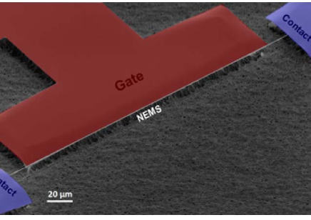
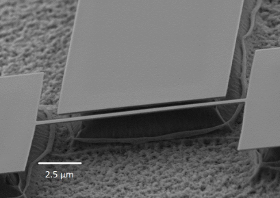
In Fig. 5 we show two Scanning Electron Micrograph (SEM) pictures of typical 300μ𝜇\leavevmode\nobreak\ \mum and 15μ𝜇\leavevmode\nobreak\ \mum devices. The gates, used in other works (e.g. [34]) are not connected in the present work. Keeping them floating or grounded is found to be equivalent.
Refer to caption
Refer to caption
Figure 5: Devices. SEM pictures of the devices. Left: 300μ𝜇\leavevmode\nobreak\ \mum beam (in false colour, the different elements of the device are indicated). Right: 15μ𝜇\leavevmode\nobreak\ \mum beam. The gates are not used in the present work.

Actuation and detection are performed with the magnetomotive scheme [43, 47]. The force amplitude acting on mode n𝑛n in the sine-wave scheme writes Fn0=ζnLBI0subscriptsuperscript𝐹0𝑛subscript𝜁𝑛𝐿𝐵subscript𝐼0F^{0}_{n}=\zeta_{n}LBI_{0} with I(t)=I0cos(ωt)𝐼𝑡subscript𝐼0𝜔𝑡I(t)=I_{0}\cos(\omega t) the drive current applied, L𝐿L the length of the beam and B𝐵B the magnetic field. ζnsubscript𝜁𝑛\zeta_{n} is a mode-dependent parameter which can be readily computed from the mode shapes (see Section 5). The detected voltage V(t)𝑉𝑡V(t) is simply the image of the velocity vn(t)subscript𝑣𝑛𝑡v_{n}(t) of the mode: V(t)=ζnLBvn(t)𝑉𝑡subscript𝜁𝑛𝐿𝐵subscript𝑣𝑛𝑡V(t)=-\zeta_{n}LB\,v_{n}(t). We detect it in a standard lock-in scheme, synchronized to the drive frequency ω𝜔\omega. We choose for commodity our definitions of the X𝑋X and Y𝑌Y quadratures of the position to match the phase of the velocity, and thus the one of the detected signal. Note that velocity vn=iωxnsubscript𝑣𝑛𝑖𝜔subscript𝑥𝑛v_{n}=i\omega\,x_{n} and displacement xnsubscript𝑥𝑛x_{n} require an additional definition: we choose the position of maximum displacement of the beam (in the first mode, it is simply the motion at the center of the beam). The actual values of the ζnsubscript𝜁𝑛\zeta_{n} coefficients obviously depend on this definition.
Refer to caption
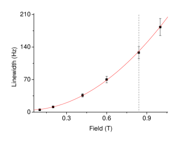
Figure 6: Loading from electric circuit. Linewidth as a function of magnetic field for device 300μ𝜇\leavevmode\nobreak\ \mum-n2. The full line is a quadratic fit (see text). The dashed vertical shows were most data have been taken.

In the magnetomotive scheme, the resonance is loaded by the impedance of the external circuit [47]. As a result, the linewidth measured presents a quadratic field dependence. We show this result for device 300μ𝜇\leavevmode\nobreak\ \mum-n2 in Fig. 6. As such, the linewidths quoted in the paper are mostly due to the electric circuit: for instance device 300μ𝜇\leavevmode\nobreak\ \mum-n2 has been measured mainly around 1 Tesla (at 0.84  T, vertical in Fig. 6). But data has also been acquired at 0.6  T and 0.42  T to verify that all features scale properly with the resonance linewidth. From the parabola in Fig. 6 one can deduce the circuit impedance as seen from the NEMS; we obtain about 2  kΩΩ\Omega which corresponds to the bias resistor plus the NEMS metallic layer resistance.

The calibration scheme we use is described in Ref. [43]. The concept on which it is based is very simple: sending a non-resonant current at frequency ωsuperscript𝜔\omega^{\prime} to the device we heat it and track the heating by means of the frequency shift of the resonance (which is T𝑇T-dependent). Doing this procedure for various ωsuperscript𝜔\omega^{\prime}, and taking the DC heating curve as reference and scaling all the others onto it, we can easily extract the transmission coefficient |G(ω)|𝐺superscript𝜔\left|G(\omega^{\prime})\right| of the injection line. This technique is very reliable: it is based on a genuinely local property, directly linked to the power injected in the nanomechanical beam. Since the aluminum on the device is non-superconducting at these temperatures, by measuring its Ohmic contribution we can then infer the transmission of the detection line.

Measuring the height xmaxsubscript𝑥𝑚𝑎𝑥x_{max} of the X peak we can easily obtain the spring constant knsubscript𝑘𝑛k_{n} of the mode through xmax=Fn0Qn/knsubscript𝑥𝑚𝑎𝑥subscriptsuperscript𝐹0𝑛subscript𝑄𝑛subscript𝑘𝑛x_{max}=F^{0}_{n}Q_{n}/k_{n} with Qn=ωn0/Δωnsubscript𝑄𝑛subscriptsuperscript𝜔0𝑛Δsubscript𝜔𝑛Q_{n}=\omega^{0}_{n}/\Delta\omega_{n} the quality factor of mode n𝑛n. From (ωn0)2=kn/mnsuperscriptsubscriptsuperscript𝜔0𝑛2subscript𝑘𝑛subscript𝑚𝑛(\omega^{0}_{n})^{2}=k_{n}/m_{n} we deduce the mass associated to the mode.
Refer to caption
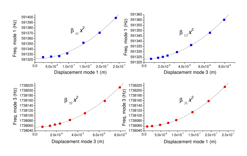
Figure 7: Nonlinear βi,jsubscript𝛽𝑖𝑗\beta_{i,j} coefficients. Measurements of the βi,jsubscript𝛽𝑖𝑗\beta_{i,j} for device 300μ𝜇\leavevmode\nobreak\ \mum-n1. The full lines correspond to quadratic fits enabling to extract the numerical values quoted in the paper.

The experimental definition of the βi,jsubscript𝛽𝑖𝑗\beta_{i,j} coefficients needed is shown in Fig. 7, for device 300μ𝜇\leavevmode\nobreak\ \mum-n1. βn,nsubscript𝛽𝑛𝑛\beta_{n,n} is obtained by measuring the position of the resonance maximum as a function of its amplitude squared, for mode n𝑛n. Driving mode n𝑛n with a strong sine-wave signal, we measure the quadratic frequency shift induced on mode m𝑚m detected with a weak sine-wave drive (such that βm,msubscript𝛽𝑚𝑚\beta_{m,m} can be neglected) [40, 39, 49]. The fit leads to coefficient βm,nsubscript𝛽𝑚𝑛\beta_{m,n}. Reversing the procedure, one obtains βn,msubscript𝛽𝑛𝑚\beta_{n,m}.

The parameters knsubscript𝑘𝑛k_{n}, mnsubscript𝑚𝑛m_{n} and βm,nsubscript𝛽𝑚𝑛\beta_{m,n} can be compared to the theoretical expectations given in Sec. 8. Typically, knsubscript𝑘𝑛k_{n} and mnsubscript𝑚𝑛m_{n} match within at most ±10plus-or-minus10\pm 10\leavevmode\nobreak\ % while the βi,jsubscript𝛽𝑖𝑗\beta_{i,j}s match within ±20plus-or-minus20\pm 20\leavevmode\nobreak\ % (which accounts for a total error on calibrations of order 10  %). In some (rare) cases, discrepancies of about ±50plus-or-minus50\pm 50\leavevmode\nobreak\ % for the nonlinear coefficients have been seen between experiment and theory. Note also that device 300μ𝜇\leavevmode\nobreak\ \mum-n1 has a frequency noticeably lower than 300μ𝜇\leavevmode\nobreak\ \mum-n2: its parameters are consistent with a slightly larger mass, certainly due to an imperfection of the beam (e.g. etching residue of silicon, inhomogeneity in shape). Typical parameters taken for the theoretical evaluation are ρSiN=3subscript𝜌𝑆𝑖𝑁3\rho_{SiN}=3\leavevmode\nobreak\ g/cm3, ESiN=200subscript𝐸𝑆𝑖𝑁200E_{SiN}=200\leavevmode\nobreak\ GPa, and in-built stress 0.90.90.9\leavevmode\nobreak\ GPa (high-stress sample), 120120120\leavevmode\nobreak\ MPa (low-stress). Note that mathematically, both types of samples are in the so-called high-stress (or string) limit. We take for the metal ρAl=2.7subscript𝜌𝐴𝑙2.7\rho_{Al}=2.7\leavevmode\nobreak\ g/cm3, EAl=50subscript𝐸𝐴𝑙50E_{Al}=50\leavevmode\nobreak\ GPa. The stess term includes thermal expansion mismatch. Computed average parameters for the composite beams are obtained from textbook results, e.g. Timoshenko’s. We summarize the experimental modal parameters in Tab. 1.

sping knsubscript𝑘𝑛k_{n} freq. ωn/2πsubscript𝜔𝑛2𝜋\omega_{n}/2\pi FWHH Δωn/2πΔsubscript𝜔𝑛2𝜋\Delta\omega_{n}/2\pi at 0.840.840.84\leavevmode\nobreak\ T non-lin. βn,m/2πsubscript𝛽𝑛𝑚2𝜋\beta_{n,m}/2\pi
n=1𝑛1n=1 device 300μ𝜇\leavevmode\nobreak\ \mum-n1 0.400.400.40\leavevmode\nobreak\ N/m 0.590.590.59\leavevmode\nobreak\ MHz 100100100\leavevmode\nobreak\ Hz β1,1=1.35 1015subscript𝛽11superscript1.351015\beta_{1,1}=1.35\,10^{15}\leavevmode\nobreak\ Hz/m2
n=1𝑛1n=1 device 300μ𝜇\leavevmode\nobreak\ \mum-n2 0.450.450.45\leavevmode\nobreak\ N/m 0.660.660.66\leavevmode\nobreak\ MHz 140140140\leavevmode\nobreak\ Hz β1,1=1.70 1015subscript𝛽11superscript1.701015\beta_{1,1}=1.70\,10^{15}\leavevmode\nobreak\ Hz/m2
n=1𝑛1n=1 device 15μ𝜇\leavevmode\nobreak\ \mum-n1 1.21.21.2\leavevmode\nobreak\ N/m 6.96.96.9\leavevmode\nobreak\ MHz 550550550\leavevmode\nobreak\ Hz β1,1=5.0 1019subscript𝛽11superscript5.01019\beta_{1,1}=5.0\,10^{19}\leavevmode\nobreak\ Hz/m2
n=3𝑛3n=3 device 300μ𝜇\leavevmode\nobreak\ \mum-n1 3.43.43.4\leavevmode\nobreak\ N/m 1.741.741.74\leavevmode\nobreak\ MHz 404040\leavevmode\nobreak\ Hz β3,1=2.75 1015subscript𝛽31superscript2.751015\beta_{3,1}=2.75\,10^{15}\leavevmode\nobreak\ Hz/m2
n=1𝑛1n=1 device 250μ𝜇\leavevmode\nobreak\ \mum-n1 0.450.450.45\leavevmode\nobreak\ N/m 0.90.90.9\leavevmode\nobreak\ MHz 190190190\leavevmode\nobreak\ Hz β1,1=8.5 1015subscript𝛽11superscript8.51015\beta_{1,1}=8.5\,10^{15}\leavevmode\nobreak\ Hz/m2
n=3𝑛3n=3 device 250μ𝜇\leavevmode\nobreak\ \mum-n1 4.04.04.0\leavevmode\nobreak\ N/m 2.72.72.7\leavevmode\nobreak\ MHz 252525\leavevmode\nobreak\ Hz β3,1=1.6 1016subscript𝛽31superscript1.61016\beta_{3,1}=1.6\,10^{16}\leavevmode\nobreak\ Hz/m2
Table 1: Measured mode parameters relevant to the data presented here. All agree fairly well with analytic computation (see text).
Refer to caption
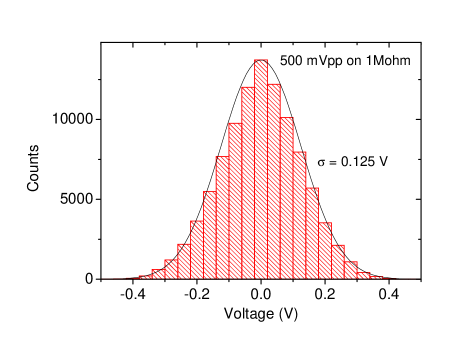
Figure 8: Gaussian noise. Characterization of Gaussian voltage noise. Histogram obtained with a large bandwidth scope; with 1  MΩΩ\Omega input. The apparatus was the HP34401A, with 0.5  Vpp/50  ΩΩ\Omega settings (delivering thus 1  Vpp on 1  MΩΩ\Omega). The line is a Gaussian fit with σ=0.125𝜎0.125\sigma=0.125\leavevmode\nobreak\ V.

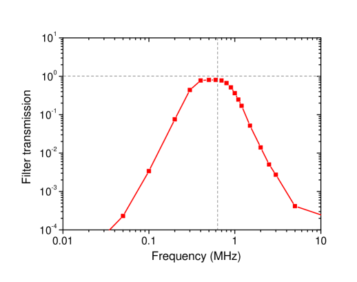
A key in our work is the careful calibration of the noise level. We used two voltage AWG (Agilent HP34401A and Tektronix AFG3252), in noise mode, which were both calibrated. The case of the HP34401A is presented in Fig. 8. We first check that the noise is indeed Gaussian, and centered, with a large bandwidth scope. We find the conversion factor from applied voltage (in Vpp) to standard deviation σ𝜎\sigma. This is performed in high-impedance mode, since the setup itself is high impedance (as opposed to 50  ΩΩ\Omega). We then verify with a spectrum analyser (and our lock-in technique, see below) that the spectrum is flat up to the generator cutoff frequency ωcsubscript𝜔𝑐\omega_{c} (about 2π×2\pi\times 10  MHz for the Agilent and 150  MHz for the Tektronix). By definition, this cutoff is chosen such that the noise spectrum writes SV(ω)=π×σ2/ωcsubscript𝑆𝑉𝜔𝜋superscript𝜎2subscript𝜔𝑐S_{V}(\omega)=\pi\times\sigma^{2}/\omega_{c} in V2/(Rad/s) (the π𝜋\pi comes from standard Fourier Transform (FT) definitions). However, typically from DC to MegaHertz there is a tiny slope which accounts for about 5  % losses in amplitude. The home made filter is also measured experimentally using a sine-wave signal and both the scope and the lock-in (Fig. 9). It is essentially flat from 0.4  MHz to 0.75  MHz, with an insertion loss of -10  % in amplitude (for our 0.6  MHz devices; similar properties apply to the shorter beam resonating around 7  MHz using another filter [11]).
Refer to caption
Figure 9: Home made filter. Transmission through our home-made filter. The curve is obtained from the ratio of input sine-wave drive amplitude to output sine-wave signal amplitude, in high-impedance mode. The dashed vertical represents the frequency of mode n=1𝑛1n=1 of our 300μ𝜇\leavevmode\nobreak\ \mum beams. Note that the mode linewidth Δω1Δsubscript𝜔1\Delta\omega_{1} is much smaller than the bandwidth of the filter.

We can easily convert the noise voltage drive into a noise current δI(t)𝛿𝐼𝑡\delta I(t), and then in turn into a noise force δFn(t)=ζnLBδI(t)𝛿subscript𝐹𝑛𝑡subscript𝜁𝑛𝐿𝐵𝛿𝐼𝑡\delta F_{n}(t)=\zeta_{n}LB\delta I(t) onto mode n𝑛n. The force noise correlator is then CFn(τ)=δFn(t)δFn(t+τ)superscriptsubscript𝐶𝐹𝑛𝜏delimited-⟨⟩𝛿subscript𝐹𝑛𝑡𝛿subscript𝐹𝑛𝑡𝜏C_{F}^{n}(\tau)=\left\langle\delta F_{n}(t)\delta F_{n}(t+\tau)\right\rangle and the spectrum SFn(ω)=FT[CFn](ω)superscriptsubscript𝑆𝐹𝑛𝜔FTdelimited-[]superscriptsubscript𝐶𝐹𝑛𝜔S_{F}^{n}(\omega)=\mathrm{FT}[C_{F}^{n}](\omega), thus SFn(ω)=(ζnLB)2SI(ω)superscriptsubscript𝑆𝐹𝑛𝜔superscriptsubscript𝜁𝑛𝐿𝐵2subscript𝑆𝐼𝜔S_{F}^{n}(\omega)=(\zeta_{n}LB)^{2}\,S_{I}(\omega). By construction, we only need to evaluate SI(ω)subscript𝑆𝐼𝜔S_{I}(\omega) within the bandwidth of the filter, where mode n=1𝑛1n=1 is excited. Elsewhere, the current is almost zero thus SFm(ω)0superscriptsubscript𝑆𝐹𝑚𝜔0S_{F}^{m}(\omega)\approx 0 for mn𝑚𝑛m\neq n.

In order to measure the Brownian motion, we designed a straightforward technique converting our lock-in into a (phase-resolved) spectrum analyser. The aim of this technique is to be able to keep all our calibrations methods the same from sine-wave measurements to noise measurements, enabling us to be as quantitative as possible. Furthermore, this noise measurement being phase-resolved, it should enable to detect any deviation from perfectly Gaussian statistics. The signal δU(t)𝛿𝑈𝑡\delta U(t) that arrives at the level of the lock-in is in fact composed of four terms: (1) the actual δV(t)=ζnLBδvn(t)𝛿𝑉𝑡subscript𝜁𝑛𝐿𝐵𝛿subscript𝑣𝑛𝑡\delta V(t)=-\zeta_{n}LB\,\delta v_{n}(t) to be studied generated by δFn(t)𝛿subscript𝐹𝑛𝑡\delta F_{n}(t), (2) an Ohmic component ReqδI(t)subscript𝑅𝑒𝑞𝛿𝐼𝑡R_{eq}\delta I(t) plus (3) a capacitive component δI(t)/Ceq𝑑t𝛿𝐼𝑡subscript𝐶𝑒𝑞differential-d𝑡\int\delta I(t)/C_{eq}\,dt, and finally (4) all other sources of noise δUnoise(t)𝛿subscript𝑈𝑛𝑜𝑖𝑠𝑒𝑡\delta U_{noise}(t) at the level of the detection which are not correlated to the current δI(t)𝛿𝐼𝑡\delta I(t). The three last components of the signal are called backgrounds, and arise from the wiring of the experiment (the resistive metallic layer, the transmission line itself from 4.2  K to room temperature and the amplifier noise). Reqsubscript𝑅𝑒𝑞R_{eq} and Ceqsubscript𝐶𝑒𝑞C_{eq} are the series transform of the actual setup as seen from the lock-in, and can be estimated from known circuit parameters. Making a RWT on the noise current, we write δI(t)=δIc(t)cos(ωt)δIs(t)sin(ωt)𝛿𝐼𝑡𝛿superscript𝐼𝑐𝑡𝜔𝑡𝛿superscript𝐼𝑠𝑡𝜔𝑡\delta I(t)=\delta I^{c}(t)\cos(\omega t)-\delta I^{s}(t)\sin(\omega t) and similarly for other variables. δvn(t)𝛿subscript𝑣𝑛𝑡\delta v_{n}(t) is readily calculated from the mechanical susceptibility relation δxn(t)=χn(t)δFn(t)𝛿subscript𝑥𝑛𝑡subscript𝜒𝑛𝑡𝛿subscript𝐹𝑛𝑡\delta x_{n}(t)=\chi_{n}(t)\ast\delta F_{n}(t). The total signal δU(t)𝛿𝑈𝑡\delta U(t) is thus:

δU(t)𝛿𝑈𝑡\displaystyle\delta U(t) =\displaystyle= ((ζnLB)2[+ωIm[χn(ω)]δIc(t)ωRe[χn(ω)]δIs(t)]+ReqδIc(t)+δIs(t)Ceqω+δUnoisec)cos(ωt)superscriptsubscript𝜁𝑛𝐿𝐵2delimited-[]𝜔𝐼𝑚delimited-[]subscript𝜒𝑛𝜔𝛿superscript𝐼𝑐𝑡𝜔𝑅𝑒delimited-[]subscript𝜒𝑛𝜔𝛿superscript𝐼𝑠𝑡subscript𝑅𝑒𝑞𝛿superscript𝐼𝑐𝑡𝛿superscript𝐼𝑠𝑡subscript𝐶𝑒𝑞𝜔𝛿superscriptsubscript𝑈𝑛𝑜𝑖𝑠𝑒𝑐𝜔𝑡\displaystyle\left(-(\zeta_{n}LB)^{2}\,\left[+\omega Im[\chi_{n}(\omega)]\delta I^{c}(t)-\omega Re[\chi_{n}(\omega)]\delta I^{s}(t)\right]+R_{eq}\delta I^{c}(t)+\frac{\delta I^{s}(t)}{C_{eq}\omega}+\delta U_{noise}^{c}\right)\cos(\omega t) (8)
\displaystyle\!\!\!\!\!\!\!\!\!\!\!\!\!\!\!\!\!\!\!\!\!- ((ζnLB)2[+ωRe[χn(ω)]δIc(t)+ωIm[χn(ω)]δIs(t)]+ReqδIs(t)δIc(t)Ceqω+δUnoises)sin(ωt),superscriptsubscript𝜁𝑛𝐿𝐵2delimited-[]𝜔𝑅𝑒delimited-[]subscript𝜒𝑛𝜔𝛿superscript𝐼𝑐𝑡𝜔𝐼𝑚delimited-[]subscript𝜒𝑛𝜔𝛿superscript𝐼𝑠𝑡subscript𝑅𝑒𝑞𝛿superscript𝐼𝑠𝑡𝛿superscript𝐼𝑐𝑡subscript𝐶𝑒𝑞𝜔𝛿superscriptsubscript𝑈𝑛𝑜𝑖𝑠𝑒𝑠𝜔𝑡\displaystyle\!\!\!\!\!\!\!\!\!\!\!\!\!\!\left(-(\zeta_{n}LB)^{2}\,\left[+\omega Re[\chi_{n}(\omega)]\delta I^{c}(t)+\omega Im[\chi_{n}(\omega)]\delta I^{s}(t)\right]+R_{eq}\delta I^{s}(t)-\frac{\delta I^{c}(t)}{C_{eq}\omega}+\delta U_{noise}^{s}\right)\sin(\omega t),

neglecting the derivatives of slow terms δI˙c(t)𝛿superscript˙𝐼𝑐𝑡\delta\dot{I}^{c}(t), δI˙s(t)𝛿superscript˙𝐼𝑠𝑡\delta\dot{I}^{s}(t) with respect to ωδIc(t)𝜔𝛿superscript𝐼𝑐𝑡\omega\delta I^{c}(t), ωδIs(t)𝜔𝛿superscript𝐼𝑠𝑡\omega\delta I^{s}(t). By definition the susceptibility terms write Re[χn(ω)]=1mn(ωn2ω2)/[(ωn2ω2)2+(Δωnω)2]𝑅𝑒delimited-[]subscript𝜒𝑛𝜔1subscript𝑚𝑛superscriptsubscript𝜔𝑛2superscript𝜔2delimited-[]superscriptsuperscriptsubscript𝜔𝑛2superscript𝜔22superscriptΔsubscript𝜔𝑛𝜔2Re[\chi_{n}(\omega)]=\frac{1}{m_{n}}(\omega_{n}^{2}-\omega^{2})/\left[(\omega_{n}^{2}-\omega^{2})^{2}+(\Delta\omega_{n}\,\omega)^{2}\right] and Im[χn(ω)]=1mn(Δωnω)/[(ωn2ω2)2+(Δωnω)2]𝐼𝑚delimited-[]subscript𝜒𝑛𝜔1subscript𝑚𝑛Δsubscript𝜔𝑛𝜔delimited-[]superscriptsuperscriptsubscript𝜔𝑛2superscript𝜔22superscriptΔsubscript𝜔𝑛𝜔2Im[\chi_{n}(\omega)]=\frac{1}{m_{n}}(-\Delta\omega_{n}\,\omega)/\left[(\omega_{n}^{2}-\omega^{2})^{2}+(\Delta\omega_{n}\,\omega)^{2}\right] in the linear response limit, when the Duffing term can be neglected. Calling δUc(t)𝛿superscript𝑈𝑐𝑡\delta U^{c}(t) and δUs(t)𝛿superscript𝑈𝑠𝑡\delta U^{s}(t) the two components in parenthesis in Eq. (8), it is straightforward to compute the correlators δUc(t)δUc(t+τ)delimited-⟨⟩𝛿superscript𝑈𝑐𝑡𝛿superscript𝑈𝑐𝑡𝜏\left\langle\delta U^{c}(t)\delta U^{c}(t+\tau)\right\rangle, δUs(t)δUs(t+τ)delimited-⟨⟩𝛿superscript𝑈𝑠𝑡𝛿superscript𝑈𝑠𝑡𝜏\left\langle\delta U^{s}(t)\delta U^{s}(t+\tau)\right\rangle and δUc(t)δUs(t+τ)delimited-⟨⟩𝛿superscript𝑈𝑐𝑡𝛿superscript𝑈𝑠𝑡𝜏\left\langle\delta U^{c}(t)\delta U^{s}(t+\tau)\right\rangle and take their Fourier Transform. One readily obtains:

Sc,c(ω)superscript𝑆𝑐𝑐𝜔\displaystyle S^{c,c}(\omega) =\displaystyle= +(ζnLB)4ω2[Re[χn(ω)]2+Im[χn(ω)]2]SI(ω)superscriptsubscript𝜁𝑛𝐿𝐵4superscript𝜔2delimited-[]𝑅𝑒superscriptdelimited-[]subscript𝜒𝑛𝜔2𝐼𝑚superscriptdelimited-[]subscript𝜒𝑛𝜔2subscript𝑆𝐼𝜔\displaystyle+(\zeta_{n}LB)^{4}\omega^{2}\left[Re[\chi_{n}(\omega)]^{2}+Im[\chi_{n}(\omega)]^{2}\right]\,S_{I}(\omega) (9)
+\displaystyle+ (ζnLB)2ω[2ReqIm[χn(ω)]+21CeqωRe[χn(ω)]]SI(ω)superscriptsubscript𝜁𝑛𝐿𝐵2𝜔delimited-[]2subscript𝑅𝑒𝑞𝐼𝑚delimited-[]subscript𝜒𝑛𝜔21subscript𝐶𝑒𝑞𝜔𝑅𝑒delimited-[]subscript𝜒𝑛𝜔subscript𝑆𝐼𝜔\displaystyle(\zeta_{n}LB)^{2}\omega\left[-2R_{eq}Im[\chi_{n}(\omega)]+2\frac{1}{C_{eq}\omega}Re[\chi_{n}(\omega)]\right]\,S_{I}(\omega)
+\displaystyle+ [(Req)2+(1Ceqω)2]SI(ω)+SδUnoise(ω),delimited-[]superscriptsubscript𝑅𝑒𝑞2superscript1subscript𝐶𝑒𝑞𝜔2subscript𝑆𝐼𝜔subscript𝑆𝛿subscript𝑈𝑛𝑜𝑖𝑠𝑒𝜔\displaystyle\left[\left(R_{eq}\right)^{2}+\left(\frac{1}{C_{eq}\omega}\right)^{2}\right]\,S_{I}(\omega)+S_{\delta U_{noise}}(\omega),
Ss,s(ω)superscript𝑆𝑠𝑠𝜔\displaystyle S^{s,s}(\omega) =\displaystyle= Sc,c(ω),superscript𝑆𝑐𝑐𝜔\displaystyle S^{c,c}(\omega), (10)
Sc,s(ω)superscript𝑆𝑐𝑠𝜔\displaystyle S^{c,s}(\omega) =\displaystyle= 0,0\displaystyle 0, (11)

having used the properties of the injected noise current, of spectrum SI(ω)subscript𝑆𝐼𝜔S_{I}(\omega), white and uncorrelated between the two identical quadratures (the amplifier noise is also assumed regular, of spectrum SδUnoise[ω]subscript𝑆𝛿subscript𝑈𝑛𝑜𝑖𝑠𝑒delimited-[]𝜔S_{\delta U_{noise}}[\omega]). The sought information is in Eq. (9), first term, with |χn(ω)|2=Re[χn(ω)]2+Im[χn(ω)]2superscriptsubscript𝜒𝑛𝜔2𝑅𝑒superscriptdelimited-[]subscript𝜒𝑛𝜔2𝐼𝑚superscriptdelimited-[]subscript𝜒𝑛𝜔2\left|\chi_{n}(\omega)\right|^{2}=Re[\chi_{n}(\omega)]^{2}+Im[\chi_{n}(\omega)]^{2}. But the measurement contains also a cross-term between mechanics and background (second term), and a pure background component (last term). Eq. (9) can be rewritten:

Sc,c(ω)superscript𝑆𝑐𝑐𝜔\displaystyle S^{c,c}(\omega) =\displaystyle= {+(ζnLB)4ω2|χn(ω)|22Req(ζnLB)2ωIm[χn(ω)]}SI(ω)superscriptsubscript𝜁𝑛𝐿𝐵4superscript𝜔2superscriptsubscript𝜒𝑛𝜔22subscript𝑅𝑒𝑞superscriptsubscript𝜁𝑛𝐿𝐵2𝜔𝐼𝑚delimited-[]subscript𝜒𝑛𝜔subscript𝑆𝐼𝜔\displaystyle\left\{+(\zeta_{n}LB)^{4}\omega^{2}\left|\chi_{n}(\omega)\right|^{2}-2R_{eq}(\zeta_{n}LB)^{2}\omega\,Im[\chi_{n}(\omega)]\right\}\,S_{I}(\omega) (12)
+\displaystyle+ {21Ceqω(ζnLB)2ωRe[χn(ω)]}SI(ω)21subscript𝐶𝑒𝑞𝜔superscriptsubscript𝜁𝑛𝐿𝐵2𝜔𝑅𝑒delimited-[]subscript𝜒𝑛𝜔subscript𝑆𝐼𝜔\displaystyle\left\{2\frac{1}{C_{eq}\omega}(\zeta_{n}LB)^{2}\omega\,Re[\chi_{n}(\omega)]\right\}\,S_{I}(\omega)
+\displaystyle+ [(Req)2+(1Ceqω)2]SI(ω)+SδUnoise(ω).delimited-[]superscriptsubscript𝑅𝑒𝑞2superscript1subscript𝐶𝑒𝑞𝜔2subscript𝑆𝐼𝜔subscript𝑆𝛿subscript𝑈𝑛𝑜𝑖𝑠𝑒𝜔\displaystyle\left[\left(R_{eq}\right)^{2}+\left(\frac{1}{C_{eq}\omega}\right)^{2}\right]\,S_{I}(\omega)+S_{\delta U_{noise}}(\omega).

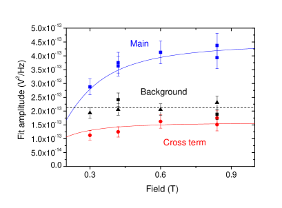
The first term is a peak, maximum at resonance, that we call the main term. The second is an imprint of the quadrature signal which is zero on resonance (we call it cross term). Finally the last term is a true background, non-mechanical, independent of field. Note that because of the loading effect which generates a peak width B2proportional-toabsentsuperscript𝐵2\propto B^{2}, the two first components tend towards a constant for large fields, with the main contribution having a stronger B4superscript𝐵4B^{4} growth.

Refer to caption
Figure 10: Fit of spectral components vs field. Data taken on sample 300μ𝜇\leavevmode\nobreak\ \mum-n2, for a noise drive current of 2.8 1019superscript2.810192.8\,10^{-19}\leavevmode\nobreak\ A2/Hz. Fit parameters are discussed below, and can be related to circuit parameters.

These components are fit on the data in Fig. 10. The fit is consistent with a model circuit of a 500ΩΩ\leavevmode\nobreak\ \Omega NEMS series resistance in parallel with 500  pF of coaxial line capacitance. These values are within a factor of 222 from actual circuit parameters, as is the overall measured background magnitude. This discrepancy is expected in the present wiring of the setup, because of the direct cross-talk (distributed along the lines) from injection signal to detection signal that affects the background detection level. At large fields, the main contribution is thus essentially |χn(ω)|2proportional-toabsentsuperscriptsubscript𝜒𝑛𝜔2\propto\left|\chi_{n}(\omega)\right|^{2}, which defines the position spectra S(ω)𝑆𝜔S(\omega) presented in this work.

Refer to caption
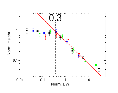
Figure 11: Measured peak height versus lock-in bandwidth. Height of the motion spectra normalized to its maximum value, with respect to the bandwidth of the lock-in detection normalized to the mechanical linewidth (Sample 300μ𝜇\leavevmode\nobreak\ \mum-n2 same current noise as Fig. 10). The different colors correspond to different field loadings: black 0.84  T, blue 0.6  T, green 0.42  T and red 0.3  T. Over this range the resonance FWHH changes from 140  Hz to 20  Hz. The lines are guides, with a crossover around 0.3.

In practice, the lock-in measurement is simply equivalent to a phase-resolved spectrum analyser. As such, the bandwidth BW𝐵𝑊BW with which the data is acquired is a key parameter. We proceed by digitizing for each given settings (drive, frequency) both X and Y signals demodulated at ω𝜔\omega on a Ni-DAQ card which is much faster than the lock-in filter itself (typ. 100  kHz). We take rather long traces (typ. few thousand points N𝑁N) from which we can calculate the auto-correlators CX(j)=<XiXi+j>subscript𝐶𝑋𝑗expectationsubscript𝑋𝑖subscript𝑋𝑖𝑗C_{X}(j)=<X_{i}\,X_{i+j}>, CY(j)=<YiYi+j>subscript𝐶𝑌𝑗expectationsubscript𝑌𝑖subscript𝑌𝑖𝑗C_{Y}(j)=<Y_{i}\,Y_{i+j}>, and the cross-correlator CXY(j)=<XiYi+j>subscript𝐶𝑋𝑌𝑗expectationsubscript𝑋𝑖subscript𝑌𝑖𝑗C_{XY}(j)=<X_{i}\,Y_{i+j}> (with <>=i/Nexpectationsubscript𝑖𝑁<\cdots>=\sum_{i}\cdots/N using cyclic index notations when i+j>N𝑖𝑗𝑁i+j>N). The Stanford SR 844 filter is used with the 242424\leavevmode\nobreak\ dB/oct. option, and from the chosen time-constant we compute the effective bandwidth BW𝐵𝑊BW of the detector. By definition SX(ω)=πCX(0)/BWsubscript𝑆𝑋𝜔𝜋subscript𝐶𝑋0𝐵𝑊S_{X}(\omega)=\pi\,C_{X}(0)/BW, SY(ω)=πCY(0)/BWsubscript𝑆𝑌𝜔𝜋subscript𝐶𝑌0𝐵𝑊S_{Y}(\omega)=\pi\,C_{Y}(0)/BW and SXY(ω)=πCXY(0)/BWsubscript𝑆𝑋𝑌𝜔𝜋subscript𝐶𝑋𝑌0𝐵𝑊S_{XY}(\omega)=\pi\,C_{XY}(0)/BW. When the statistics is regular, we find SX(ω)=SY(ω)subscript𝑆𝑋𝜔subscript𝑆𝑌𝜔S_{X}(\omega)=S_{Y}(\omega) and SXY(ω)=0subscript𝑆𝑋𝑌𝜔0S_{XY}(\omega)=0 as we should (see Section 7).

Refer to caption
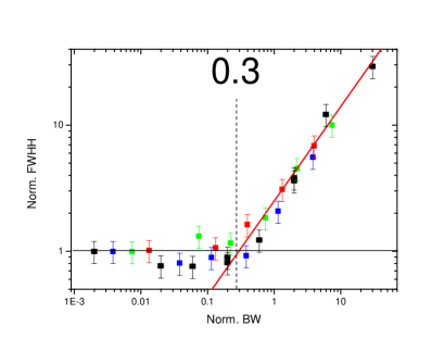
Figure 12: Measured peak width versus lock-in bandwidth. FWHH of the motion spectra normalized to its minimum value, with respect to the bandwidth of the lock-in detection normalized to the mechanical linewidth (same conditions as Fig. 11). Conventions are the same as in the previous graph.

The effect of the bandwidth BW𝐵𝑊BW is twofold: on one hand (1) the larger it is, the more noise is collected by the lock-in and thus the larger the detected signal CX(0)subscript𝐶𝑋0C_{X}(0) is. However, (2) when the bandwidth is large compared to the width of the mechanical resonance, then the true mechanical signal is “diluted” within the background. As a result, the measured peak height decreases with respect to the background, and broadens; this is shown on both Figs. 11 and 12. At the same time, the background simply scales as the bandwith, as it should for a white noise. On these graphs, we represent the heights and FWHH of the resonance peak normalized to their actual value with respect to the BW𝐵𝑊BW of the lock-in detection normalized to the mechanical resonance linewidth ΔωΔ𝜔\Delta\omega. We see that the best trade-off is around BW0.3Δωn𝐵𝑊0.3Δsubscript𝜔𝑛BW\approx 0.3\leavevmode\nobreak\ \Delta\omega_{n}, where signal is rather large without a strong impact on the measured peak.

Refer to caption
Figure 13: Measured Brownian motion versus applied stochastic force. Measured standard deviation Δx12Δsuperscriptsubscript𝑥12\Delta x_{1}^{2} for sample 300μ𝜇\leavevmode\nobreak\ \mum-n2 at 0.84  T with respect to applied force noise (varying the noise current intensity). The line is the theoretical calculation (see text). On the right vertical axis, the motion is converted into effective temperature for mode n=1𝑛1n=1.

When the noise is not too large on mode n𝑛n, the Duffing non-linearity is negligible and the mechanical spectrum is a Lorentzian peak. Its area is proportional to Height×\leavevmode\nobreak\ \times\leavevmode\nobreak\ FWHH, and is directly related to the standard deviation Δxn2Δsuperscriptsubscript𝑥𝑛2\Delta x_{n}^{2} of the mode position fluctuations. Furthermore, Δxn2Δsuperscriptsubscript𝑥𝑛2\Delta x_{n}^{2} is directly linked to the applied force noise through Δxn2=SFnQnωn/(2kn2)Δsuperscriptsubscript𝑥𝑛2superscriptsubscript𝑆𝐹𝑛subscript𝑄𝑛subscript𝜔𝑛2superscriptsubscript𝑘𝑛2\Delta x_{n}^{2}=S_{F}^{n}\,Q_{n}\omega_{n}/(2k_{n}^{2}). This relation is shown in Fig. 13, together with computed effective temperatures.

When the force noise becomes large, then the Duffing term is not negligible anymore: the spectrum becomes a “Duffing spectrum” (Fig. 2 of paper and Fig. 14 below). However, for high-Q devices one can show solving the Fokker-Planck equation that the statistics remains Gaussian [45]. Indeed, no anomalies are seen on the measured spectra (we still have SX(ω)=SY(ω)subscript𝑆𝑋𝜔subscript𝑆𝑌𝜔S_{X}(\omega)=S_{Y}(\omega) and SXY(ω)=0subscript𝑆𝑋𝑌𝜔0S_{XY}(\omega)=0, see Section 7). Furthermore, since the measured peak is nothing but the convolution of the mechanical susceptibility with a “distribution” generated by the fluctuations, see Section 6, the area of this peak is preserved: thus the above proportionality relation between measured Δxn2Δsuperscriptsubscript𝑥𝑛2\Delta x_{n}^{2} and force spectrum SFnsuperscriptsubscript𝑆𝐹𝑛S_{F}^{n} still applies for the distorted spectra. This can be seen experimentally at very large effective temperatures in Fig. 13. Physically, this simply comes from the fact that the induced frequency noise by the non-linear term is purely dispersive, and no extra energy is transferred from the mode to the environment. Note that even though the line distorts, the Height×\leavevmode\nobreak\ \times\leavevmode\nobreak\ FWHH remains a rather good estimate of the area of the peak. For the sake of completeness, we should mention that for noise levels above about Δx124. 1014Δsuperscriptsubscript𝑥12superscript4.1014\Delta x_{1}^{2}\approx 4.\,10^{-14}\leavevmode\nobreak\ m2, we do see a Joule heating of the structure due to the large currents injected in the aluminum layer. It is easy to correct for this effect, which produces here only a tiny negative frequency shift which is calibrated in the first place [43].

Finally, let us comment the range of effective temperatures explored in this experiment. Even though the smallest stochastic drives already correspond to about 100 000100000100\,000\leavevmode\nobreak\ Kelvin, they lie within the “motional narrowing” limit (see analytical expansions in Section 6, Figs. 3 & 17 and final discussion on actual thermal bath Section 8). On the other hand, the highest levels of noise used are extremely high and lie in the “inhomogeneous broadening” range: nonetheless, the basic properties of position fluctuations are not altered (Gaussianity, preserved stored energy in the resonance i.e. the expression of the equipartition theorem here). One needs quite peculiar conditions to destroy these properties, and e.g. create squeezed statistics. This is what can be achieved by adding a large sine-wave excitation force on the same mode where large fluctuations are present (see Section 7).

5 Non-linear mode coupling

The basic starting point is the Euler-Bernoulli equation in which the non-linear effect of tensioning has been incorporated [49]. It has been discussed extensively in the literature already [40, 39], and we just remind the maths here. The equation writes:

ρbeamA2u(z,t)t2+η[u(z,t)]t+EbeamIz4u(z,t)z4[T0+EbeamA2L0L(u(z,t)z)2𝑑z]2u(z,t)z2=F(z,t)z,subscript𝜌𝑏𝑒𝑎𝑚𝐴superscript2𝑢𝑧𝑡superscript𝑡2𝜂delimited-[]𝑢𝑧𝑡𝑡subscript𝐸𝑏𝑒𝑎𝑚subscript𝐼𝑧superscript4𝑢𝑧𝑡superscript𝑧4delimited-[]subscript𝑇0subscript𝐸𝑏𝑒𝑎𝑚𝐴2𝐿subscriptsuperscript𝐿0superscript𝑢𝑧𝑡𝑧2differential-d𝑧superscript2𝑢𝑧𝑡superscript𝑧2𝐹𝑧𝑡𝑧\!\!\!\!\!\rho_{beam}A\frac{\partial^{2}u(z,t)}{\partial t^{2}}+\eta\frac{\partial{\cal L}\left[u(z,t)\right]}{\partial t}+E_{beam}\,I_{z}\frac{\partial^{4}u(z,t)}{\partial z^{4}}-\left[T_{0}+\frac{E_{beam}\,A}{2L}\int^{L}_{0}\left(\frac{\partial u(z,t)}{\partial z}\right)^{\!\!2}dz\right]\frac{\partial^{2}u(z,t)}{\partial z^{2}}=\frac{\partial F(z,t)}{\partial z}\,, (13)

with z𝑧\vec{z} the axis along the beam, L𝐿L the length, A=we𝐴𝑤𝑒A=we its cross section (w𝑤w is the width and e𝑒e the thickness), Izsubscript𝐼𝑧I_{z} its second moment of area. T0subscript𝑇0T_{0} is the stored tension, ρbeamsubscript𝜌𝑏𝑒𝑎𝑚\rho_{beam} the mass density and Ebeamsubscript𝐸𝑏𝑒𝑎𝑚E_{beam} the Young’s modulus. The parameters can be adapted to the case of a bilayer system (here Al on SiN, see e.g. Timoshenko’s textbook).

In Eq. (13), F(z,t)/z𝐹𝑧𝑡𝑧\partial F(z,t)/\partial z is the overall external force per unit length applied to the beam, and u(z,t)𝑢𝑧𝑡u(z,t) its motion in the x𝑥\vec{x} direction. We do not mention any explicit model of mechanical dissipation, and just assume that the friction force is proportional to the time-derivative of some linear functional {\cal L} of the local displacement u(z,t)𝑢𝑧𝑡u(z,t). We will limit the discussion to two modes, the extension to more being straitghforward, following the works of Refs. [39, 40, 38, 49]. Let u(z,t)=xn(t)Ψn(z)+xm(t)Ψm(z)𝑢𝑧𝑡subscript𝑥𝑛𝑡subscriptΨ𝑛𝑧subscript𝑥𝑚𝑡subscriptΨ𝑚𝑧u(z,t)=x_{n}(t)\Psi_{n}(z)+x_{m}(t)\Psi_{m}(z) with Ψn(z),Ψm(z)subscriptΨ𝑛𝑧subscriptΨ𝑚𝑧\Psi_{n}(z),\Psi_{m}(z) the mode shapes of mode n𝑛n and m𝑚m. In this modal decomposition, we take the Ψn,ΨmsubscriptΨ𝑛subscriptΨ𝑚\Psi_{n},\Psi_{m} functions to be normalized at 1 at their maximum. This defines our (time-dependent) amplitude parameters xn(t),xm(t)subscript𝑥𝑛𝑡subscript𝑥𝑚𝑡x_{n}(t),x_{m}(t).

Replacing u(z,t)𝑢𝑧𝑡u(z,t) into Eq. (13) and projecting on one of the modes (i.e. multiplying by Ψn(z)subscriptΨ𝑛𝑧\Psi_{n}(z) or Ψm(z)subscriptΨ𝑚𝑧\Psi_{m}(z) and integrating over the beam), we obtain:

ρbeamALJn,nx¨n(t)+ρbeamALJn,mx¨m(t)+ηKn,nx˙n(t)+ηKn,mx˙m(t)+ρbeamAL[(ωn0)2Jn,nx¨n(t)+(ωm0)2Jn,mx¨m(t)]subscript𝜌𝑏𝑒𝑎𝑚𝐴𝐿subscript𝐽𝑛𝑛subscript¨𝑥𝑛𝑡subscript𝜌𝑏𝑒𝑎𝑚𝐴𝐿subscript𝐽𝑛𝑚subscript¨𝑥𝑚𝑡𝜂subscript𝐾𝑛𝑛subscript˙𝑥𝑛𝑡𝜂subscript𝐾𝑛𝑚subscript˙𝑥𝑚𝑡subscript𝜌𝑏𝑒𝑎𝑚𝐴𝐿delimited-[]superscriptsuperscriptsubscript𝜔𝑛02subscript𝐽𝑛𝑛subscript¨𝑥𝑛𝑡superscriptsuperscriptsubscript𝜔𝑚02subscript𝐽𝑛𝑚subscript¨𝑥𝑚𝑡\displaystyle\!\!\!\!\!\!\!\!\!\!\!\!\!\!\!\!\!\!\!\!\!\!\!\!\!\!\!\!\!\!\!\!\!\!\!\!\!\!\rho_{beam}ALJ_{n,n}\,\ddot{x}_{n}(t)+\rho_{beam}ALJ_{n,m}\,\ddot{x}_{m}(t)+\eta K_{n,n}\,\dot{x}_{n}(t)+\eta K_{n,m}\,\dot{x}_{m}(t)+\rho_{beam}AL\left[\left(\omega_{n}^{0}\right)^{2}J_{n,n}\,\ddot{x}_{n}(t)+\left(\omega_{m}^{0}\right)^{2}J_{n,m}\,\ddot{x}_{m}(t)\right] (14)
+\displaystyle\!\!\!\!\!\!\!\!\!\!\!\!\!\!\!\!\!\!\!\!\!\!\!\!\!\!\!\!\!\!\!\!\!\!\!\!\!\!\!\!\!\!\!\!\!\!\!\!\!\!\!\!\!\!\!+ EbeamA2L3[xn(t)3In,n2+xm(t)3Im,mIn,m+xn(t)2xm(t)(3In,nIn,m)+xm(t)2xn(t)(In,nIm,m+2In,m2)]subscript𝐸𝑏𝑒𝑎𝑚𝐴2superscript𝐿3delimited-[]subscript𝑥𝑛superscript𝑡3superscriptsubscript𝐼𝑛𝑛2subscript𝑥𝑚superscript𝑡3subscript𝐼𝑚𝑚subscript𝐼𝑛𝑚subscript𝑥𝑛superscript𝑡2subscript𝑥𝑚𝑡3subscript𝐼𝑛𝑛subscript𝐼𝑛𝑚subscript𝑥𝑚superscript𝑡2subscript𝑥𝑛𝑡subscript𝐼𝑛𝑛subscript𝐼𝑚𝑚2superscriptsubscript𝐼𝑛𝑚2\displaystyle\!\!\!\!\!\!\!\!\!\!\!\!\!\!\!\!\!\!\!\!\!\!\!\!\!\!\!\!\!\!\!\frac{E_{beam}\,A}{2L^{3}}\!\!\left[x_{n}(t)^{3}I_{n,n}^{2}+x_{m}(t)^{3}I_{m,m}I_{n,m}+x_{n}(t)^{2}x_{m}(t)\left(3I_{n,n}I_{n,m}\right)+x_{m}(t)^{2}x_{n}(t)\left(I_{n,n}I_{m,m}+2I_{n,m}^{2}\right)\right]
=\displaystyle= F0Lζncos(ωt),subscript𝐹0𝐿subscript𝜁𝑛𝜔𝑡\displaystyle F_{0}L\,\zeta_{n}\,\cos(\omega t),

having assumed F(z,t)/z=F0cos(ωt)𝐹𝑧𝑡𝑧subscript𝐹0𝜔𝑡\partial F(z,t)/\partial z=F_{0}\cos(\omega t) independent of z𝑧z, and used the modal relation EbeamIzΨi′′′′T0Ψi′′=ρbeamA(ωi0)2Ψisubscript𝐸𝑏𝑒𝑎𝑚subscript𝐼𝑧superscriptsubscriptΨ𝑖′′′′subscript𝑇0superscriptsubscriptΨ𝑖′′subscript𝜌𝑏𝑒𝑎𝑚𝐴superscriptsuperscriptsubscript𝜔𝑖02subscriptΨ𝑖E_{beam}I_{z}\Psi_{i}^{{}^{\prime\prime\prime\prime}}-T_{0}\Psi_{i}^{{}^{\prime\prime}}=\rho_{beam}A\,\left(\omega_{i}^{0}\right)^{2}\Psi_{i}. ωi0superscriptsubscript𝜔𝑖0\omega_{i}^{0} is the natural resonance frequency of mode i𝑖i. The parameters introduced above are ζn=0LΨn(z)𝑑z/Lsubscript𝜁𝑛subscriptsuperscript𝐿0subscriptΨ𝑛𝑧differential-d𝑧𝐿\zeta_{n}=\int^{L}_{0}\Psi_{n}(z)dz/L, Jn,m=0LΨn(z)Ψm(z)𝑑z/Lsubscript𝐽𝑛𝑚subscriptsuperscript𝐿0subscriptΨ𝑛𝑧subscriptΨ𝑚𝑧differential-d𝑧𝐿J_{n,m}=\int^{L}_{0}\Psi_{n}(z)\Psi_{m}(z)dz/L, Kn,m=0LΨn(z)[Ψm(z)]𝑑zsubscript𝐾𝑛𝑚subscriptsuperscript𝐿0subscriptΨ𝑛𝑧delimited-[]subscriptΨ𝑚𝑧differential-d𝑧K_{n,m}=\int^{L}_{0}\Psi_{n}(z){\cal L}\left[\Psi_{m}(z)\right]dz and In,m=L0LΨn(z)Ψm(z)𝑑zsubscript𝐼𝑛𝑚𝐿subscriptsuperscript𝐿0subscriptΨ𝑛superscript𝑧subscriptΨ𝑚superscript𝑧differential-d𝑧I_{n,m}=L\int^{L}_{0}\Psi_{n}(z)^{{}^{\prime}}\Psi_{m}(z)^{{}^{\prime}}dz. Eq. (14) applies to the projection on mode n𝑛n; the projection on m𝑚m is obtained by inverting nm𝑛𝑚n\leftrightarrow m. In the ideal case, the modes are orthogonal and Jn,m=Kn,m=In,m=0subscript𝐽𝑛𝑚subscript𝐾𝑛𝑚subscript𝐼𝑛𝑚0J_{n,m}=K_{n,m}=I_{n,m}=0 when nm𝑛𝑚n\neq m. In the real case, orthogonality is not perfect; however, writing xi(t)=xi0cos(ωt+ϕ)subscript𝑥𝑖𝑡superscriptsubscript𝑥𝑖0𝜔𝑡italic-ϕx_{i}(t)=x_{i}^{0}\cos(\omega t+\phi) and using a RWT one immediately sees that many terms in Eq. (14) are off-resonant with respect to mode n𝑛n. It is thus perfectly enough to recast the above result into:

mnx¨n(t)+2λnx˙n(t)+mn(ωn0)2xn(t)+kn,nxn(t)3+kn,mxn(t)xm(t)2=Fn(t),subscript𝑚𝑛subscript¨𝑥𝑛𝑡2subscript𝜆𝑛subscript˙𝑥𝑛𝑡subscript𝑚𝑛superscriptsuperscriptsubscript𝜔𝑛02subscript𝑥𝑛𝑡subscript𝑘𝑛𝑛subscript𝑥𝑛superscript𝑡3subscript𝑘𝑛𝑚subscript𝑥𝑛𝑡subscript𝑥𝑚superscript𝑡2subscript𝐹𝑛𝑡m_{n}\,\ddot{x}_{n}(t)+2\lambda_{n}\,\dot{x}_{n}(t)+m_{n}\left(\omega_{n}^{0}\right)^{2}\,x_{n}(t)+k_{n,n}\,x_{n}(t)^{3}+k_{n,m}\,x_{n}(t)x_{m}(t)^{2}=F_{n}(t), (15)

for mode n𝑛n. An equivalent expression holds for mode m𝑚m. We have defined the mode parameters mn=ρbeamALJn,nsubscript𝑚𝑛subscript𝜌𝑏𝑒𝑎𝑚𝐴𝐿subscript𝐽𝑛𝑛m_{n}=\rho_{beam}ALJ_{n,n}, λn=ηKn,n/2subscript𝜆𝑛𝜂subscript𝐾𝑛𝑛2\lambda_{n}=\eta K_{n,n}/2 together with kn=mn(ωn0)2subscript𝑘𝑛subscript𝑚𝑛superscriptsuperscriptsubscript𝜔𝑛02k_{n}=m_{n}\left(\omega_{n}^{0}\right)^{2}. The projection of the force on the mode is Fn(t)=Fn0cos(ωt)subscript𝐹𝑛𝑡superscriptsubscript𝐹𝑛0𝜔𝑡F_{n}(t)=F_{n}^{0}\cos(\omega t) with Fn0=F0Lζnsuperscriptsubscript𝐹𝑛0subscript𝐹0𝐿subscript𝜁𝑛F_{n}^{0}=F_{0}L\zeta_{n}. Finally, the non-linear coefficients write kn,n=EbeamA2L3In,n2subscript𝑘𝑛𝑛subscript𝐸𝑏𝑒𝑎𝑚𝐴2superscript𝐿3superscriptsubscript𝐼𝑛𝑛2k_{n,n}=\frac{E_{beam}\,A}{2L^{3}}I_{n,n}^{2} and kn,m=EbeamA2L3(In,nIm,m+2In,m2)subscript𝑘𝑛𝑚subscript𝐸𝑏𝑒𝑎𝑚𝐴2superscript𝐿3subscript𝐼𝑛𝑛subscript𝐼𝑚𝑚2superscriptsubscript𝐼𝑛𝑚2k_{n,m}=\frac{E_{beam}\,A}{2L^{3}}\left(I_{n,n}I_{m,m}+2I_{n,m}^{2}\right) for nm𝑛𝑚n\neq m. Eq. (15) is noting but the driven Duffing equation (for mode n𝑛n), with an extra coupling term to mode m𝑚m. This is the formalism developed in Refs. [39, 40, 38, 49].

We turn now to the situation where Fn(t)=Fn0cos(ωt)+δFn(t)subscript𝐹𝑛𝑡superscriptsubscript𝐹𝑛0𝜔𝑡𝛿subscript𝐹𝑛𝑡F_{n}(t)=F_{n}^{0}\cos(\omega t)+\delta F_{n}(t) and Fm(t)=Fm0cos(ωt)+δFm(t)subscript𝐹𝑚𝑡superscriptsubscript𝐹𝑚0𝜔𝑡𝛿subscript𝐹𝑚𝑡F_{m}(t)=F_{m}^{0}\cos(\omega t)+\delta F_{m}(t), introducing the stochastic variables δFn(t),δFm(t)𝛿subscript𝐹𝑛𝑡𝛿subscript𝐹𝑚𝑡\delta F_{n}(t),\delta F_{m}(t). These are taken as being white, Gaussian, and uncorrelated. The obvious ansatz solving Eq. (15) consists in writing xi(t)=xi0(t)+δxi(t)subscript𝑥𝑖𝑡superscriptsubscript𝑥𝑖0𝑡𝛿subscript𝑥𝑖𝑡x_{i}(t)=x_{i}^{0}(t)+\delta x_{i}(t) for i=n,m𝑖𝑛𝑚i=n,m, with xi0(t)superscriptsubscript𝑥𝑖0𝑡x_{i}^{0}(t) a certain (and eventually sinusoidal) component and δxi(t)𝛿subscript𝑥𝑖𝑡\delta x_{i}(t) a random motion. Replacing in the above equation, we obtain:

x¨n0(t)+Δωnx˙n0(t)+(ωn0)2xn0(t)+2ωn043βn,nxn0(t)3superscriptsubscript¨𝑥𝑛0𝑡Δsubscript𝜔𝑛superscriptsubscript˙𝑥𝑛0𝑡superscriptsuperscriptsubscript𝜔𝑛02superscriptsubscript𝑥𝑛0𝑡2superscriptsubscript𝜔𝑛043subscript𝛽𝑛𝑛superscriptsubscript𝑥𝑛0superscript𝑡3\displaystyle\ddot{x}_{n}^{0}(t)+\Delta\omega_{n}\,\dot{x}_{n}^{0}(t)+\left(\omega_{n}^{0}\right)^{2}\,x_{n}^{0}(t)+2\omega_{n}^{0}\frac{4}{3}\beta_{n,n}\,x_{n}^{0}(t)^{3} (16)
+\displaystyle+ 2ωn0[+2βn,mxm0(t)2xn0(t)+4βn,nδxn(t)2xn0(t)+2βn,mδxm(t)2xn0(t)]2superscriptsubscript𝜔𝑛0delimited-[]2subscript𝛽𝑛𝑚superscriptsubscript𝑥𝑚0superscript𝑡2superscriptsubscript𝑥𝑛0𝑡4subscript𝛽𝑛𝑛𝛿subscript𝑥𝑛superscript𝑡2superscriptsubscript𝑥𝑛0𝑡2subscript𝛽𝑛𝑚𝛿subscript𝑥𝑚superscript𝑡2superscriptsubscript𝑥𝑛0𝑡\displaystyle 2\omega_{n}^{0}\left[+2\beta_{n,m}\,x_{m}^{0}(t)^{2}x_{n}^{0}(t)+4\beta_{n,n}\,\delta x_{n}(t)^{2}x_{n}^{0}(t)+2\beta_{n,m}\,\delta x_{m}(t)^{2}x_{n}^{0}(t)\right]
+\displaystyle+ δx¨n(t)+Δωnδx˙n(t)+(ωn0)2δxn(t)+2ωn043βn,nδxn(t)3𝛿subscript¨𝑥𝑛𝑡Δsubscript𝜔𝑛𝛿subscript˙𝑥𝑛𝑡superscriptsuperscriptsubscript𝜔𝑛02𝛿subscript𝑥𝑛𝑡2superscriptsubscript𝜔𝑛043subscript𝛽𝑛𝑛𝛿subscript𝑥𝑛superscript𝑡3\displaystyle\delta\ddot{x}_{n}(t)+\Delta\omega_{n}\,\delta\dot{x}_{n}(t)+\left(\omega_{n}^{0}\right)^{2}\,\delta x_{n}(t)+2\omega_{n}^{0}\frac{4}{3}\beta_{n,n}\,\delta x_{n}(t)^{3}
+\displaystyle+ 2ωn0[+2βn,mxm0(t)2δxn(t)+4βn,nxn0(t)2δxn(t)+2βn,mδxm(t)2δxn(t)]2superscriptsubscript𝜔𝑛0delimited-[]2subscript𝛽𝑛𝑚superscriptsubscript𝑥𝑚0superscript𝑡2𝛿subscript𝑥𝑛𝑡4subscript𝛽𝑛𝑛superscriptsubscript𝑥𝑛0superscript𝑡2𝛿subscript𝑥𝑛𝑡2subscript𝛽𝑛𝑚𝛿subscript𝑥𝑚superscript𝑡2𝛿subscript𝑥𝑛𝑡\displaystyle 2\omega_{n}^{0}\left[+2\beta_{n,m}x_{m}^{0}(t)^{2}\delta x_{n}(t)+4\beta_{n,n}x_{n}^{0}(t)^{2}\delta x_{n}(t)+2\beta_{n,m}\delta x_{m}(t)^{2}\delta x_{n}(t)\right]
=\displaystyle= Fn0mncos(ωt)+δFn(t)mn,superscriptsubscript𝐹𝑛0subscript𝑚𝑛𝜔𝑡𝛿subscript𝐹𝑛𝑡subscript𝑚𝑛\displaystyle\frac{F_{n}^{0}}{m_{n}}\cos(\omega t)+\frac{\delta F_{n}(t)}{m_{n}},

with Δωn=2λn/mnΔsubscript𝜔𝑛2subscript𝜆𝑛subscript𝑚𝑛\Delta\omega_{n}=2\lambda_{n}/m_{n} the linewidth parameter associated to mode n𝑛n. We introduced the Duffing parameters βn,n=34kn,n/mn2ωn0subscript𝛽𝑛𝑛34subscript𝑘𝑛𝑛subscript𝑚𝑛2superscriptsubscript𝜔𝑛0\beta_{n,n}=\frac{3}{4}\frac{k_{n,n}/m_{n}}{2\omega_{n}^{0}} and βn,m=12kn,m/mn2ωn0subscript𝛽𝑛𝑚12subscript𝑘𝑛𝑚subscript𝑚𝑛2superscriptsubscript𝜔𝑛0\beta_{n,m}=\frac{1}{2}\frac{k_{n,m}/m_{n}}{2\omega_{n}^{0}}. Note that kn,m=km,nsubscript𝑘𝑛𝑚subscript𝑘𝑚𝑛k_{n,m}=k_{m,n} but βn,mβm,nsubscript𝛽𝑛𝑚subscript𝛽𝑚𝑛\beta_{n,m}\neq\beta_{m,n}. The first line and the third line of Eq. (16) correspond to the Duffing equation written for the certain component and the stochastic one respectively. The first bracket is the non-linear coupling onto the certain dynamics: the first element xm0(t)2xn0(t)proportional-toabsentsuperscriptsubscript𝑥𝑚0superscript𝑡2superscriptsubscript𝑥𝑛0𝑡\propto x_{m}^{0}(t)^{2}x_{n}^{0}(t) is nothing but the standard mode-coupling term between mode m𝑚m and n𝑛n, while the two others correspond to the coupling of the fluctuations to the certain position variable. Note the factor of 2 between the coupling to mode m𝑚m fluctuations, and to the same mode n𝑛n. The second bracket is the equivalent mode-coupling term onto the random motion of mode n𝑛n: the two first elements depend on the certain components of m𝑚m and n𝑛n, while the last one is due to the fluctuations of mode m𝑚m. Note again the factor of 2 between “inter-mode coupling” and “self-coupling” (or “intra-mode coupling”). In the next section, we explain how to solve Eq. (16) for small sine-wave drives and give the explicit theoretical results relevant to the present work, taken from Ref. [41].

6 Adiabatic description of the noise coupling: from “motional narrowing” to “inhomogeneous broadening”

The theoretical analysis we use is the one developed in Ref. [41]. Here, we quickly describe the maths leading to the analytic solution of the problem studied. The first step is to write the dynamics equation Eq. (16) in the frame rotating at the speed of the mode’s oscillation. The transformed motion variable x~n0(t)superscriptsubscript~𝑥𝑛0𝑡\tilde{x}_{n}^{0}(t) writes xn0(t)=(x~n0(t)Exp[iωn0t]+x~n0(t)Exp[iωn0t])/2superscriptsubscript𝑥𝑛0𝑡superscriptsubscript~𝑥𝑛0𝑡Expdelimited-[]𝑖superscriptsubscript𝜔𝑛0𝑡superscriptsubscript~𝑥𝑛0𝑡Expdelimited-[]𝑖superscriptsubscript𝜔𝑛0𝑡2x_{n}^{0}(t)=(\tilde{x}_{n}^{0}(t)\mathrm{Exp}[i\omega_{n}^{0}t]+\tilde{x}_{n}^{0\,\ast}(t)\mathrm{Exp}[-i\omega_{n}^{0}t])/2. Making a Rotating Wave Approximation (RWA), the component of the frequency fluctuations δxn(t)2proportional-toabsent𝛿subscript𝑥𝑛superscript𝑡2\propto\delta x_{n}(t)^{2} at 2ωn2subscript𝜔𝑛2\omega_{n} is removed, keeping only its slow dynamics (and static average). Note that this high-frequency term corresponds somehow to a “random parametric pumping” for the certain dynamics xn0superscriptsubscript𝑥𝑛0x_{n}^{0} of mode n𝑛n; but one can show nonetheless that its impact is negligible, and can be safely neglected.

Thus, the dynamics of the certain component adiabatically follows the slow fluctuations, which can be interpreted as phase diffusion for the resonator. As such, the final result of the averaging of this phase diffusion can be written in time-domain as a multiplication of the mode’s decay function by an expression which Fourier Transform we call a “frequency distribution” (in frequency-domain). This is not strictly speaking a frequency distribution, since in the “motional narrowing” limit it is complex-valued.

Let us briefly remind the reader of the approach followed by Zhang and Dykman in Ref. [41]. To simplify the discussion, we neglect for the time being the intra-mode non-linearity. Nonetheless, the following approach can be extended without loss of generality to the intra-mode case, provided that the driven motion is not too high. Under this assumption, the fluctuations of the driven mode and its certain component can be linearly separated. The linearized NEMS’ dynamics equations for modes n𝑛n (driven, i.e. the probe mode) and m𝑚m (noisy, undriven) in the RWA, are then:

δx~˙m(t)+Δωm2δx~m(t)=δFm(t)eiωmt2mmωm,subscript˙𝛿~𝑥𝑚𝑡Δsubscript𝜔𝑚2𝛿subscript~𝑥𝑚𝑡𝛿subscript𝐹𝑚𝑡superscript𝑒𝑖subscript𝜔𝑚𝑡2subscript𝑚𝑚subscript𝜔𝑚\dot{\delta\tilde{x}}_{m}(t)+\frac{\Delta\omega_{m}}{2}\delta\tilde{x}_{m}(t)=\frac{\delta F_{m}(t)e^{-i\omega_{m}t}}{2m_{m}\omega_{m}}, (17)
x~˙n0(t)+(Δωn2+i[ωωnδω(t)])x~n0(t)=Fn0eiϕ4mnωn,superscriptsubscript˙~𝑥𝑛0𝑡Δsubscript𝜔𝑛2𝑖delimited-[]𝜔subscript𝜔𝑛𝛿𝜔𝑡superscriptsubscript~𝑥𝑛0𝑡superscriptsubscript𝐹𝑛0superscript𝑒𝑖italic-ϕ4subscript𝑚𝑛subscript𝜔𝑛\dot{\tilde{x}}_{n}^{0}(t)+\left(\frac{\Delta\omega_{n}}{2}+i[\omega-\omega_{n}-\delta\omega(t)]\right)\tilde{x}_{n}^{0}(t)=\frac{F_{n}^{0}e^{i\phi}}{4m_{n}\omega_{n}}, (18)

with δωn(t)=βn,m|δx~m0(t)|2=βn,m[δXm(t)2+δYm(t)2]𝛿subscript𝜔𝑛𝑡subscript𝛽𝑛𝑚superscript𝛿superscriptsubscript~𝑥𝑚0𝑡2subscript𝛽𝑛𝑚delimited-[]𝛿subscript𝑋𝑚superscript𝑡2𝛿subscript𝑌𝑚superscript𝑡2\delta\omega_{n}(t)=\beta_{n,m}|\delta\tilde{x}_{m}^{0}(t)|^{2}=\beta_{n,m}\left[\delta X_{m}(t)^{2}+\delta Y_{m}(t)^{2}\right], where δXm,δYm𝛿subscript𝑋𝑚𝛿subscript𝑌𝑚\delta X_{m},\delta Y_{m} are the quadratures of the fluctuating mode’s motion. Integrating Eq.(18), we obtain the response of the slow variable in the time domain, which is stochastic:

x~n0(t)=tFn0eiϕ4mnωnexp([Δωn2+i(ωωn)](tt)+ittδω(t′′)dt′′)dt.superscriptsubscript~𝑥𝑛0𝑡superscriptsubscript𝑡superscriptsubscript𝐹𝑛0superscript𝑒𝑖italic-ϕ4subscript𝑚𝑛subscript𝜔𝑛delimited-[]Δsubscript𝜔𝑛2𝑖𝜔subscript𝜔𝑛𝑡superscript𝑡𝑖superscriptsubscriptsuperscript𝑡𝑡𝛿𝜔superscript𝑡′′differential-dsuperscript𝑡′′differential-dsuperscript𝑡\tilde{x}_{n}^{0}(t)=\int_{-\infty}^{t}\frac{F_{n}^{0}e^{i\phi}}{4m_{n}\omega_{n}}\exp\left(-\left[\frac{\Delta\omega_{n}}{2}+i(\omega-\omega_{n})\right](t-t^{\prime})+i\int_{t^{\prime}}^{t}\delta\omega(t^{\prime\prime})\mathrm{d}t^{\prime\prime}\right)\mathrm{d}t^{\prime}. (19)

The exponential term is nothing but a stochastic susceptibility in the time domain χsl(t,t)subscript𝜒𝑠𝑙𝑡superscript𝑡\chi_{sl}(t,t^{\prime}):

x~n0(t)=tFn0eiϕ4mnωnχsl(t,t)dt,superscriptsubscript~𝑥𝑛0𝑡superscriptsubscript𝑡superscriptsubscript𝐹𝑛0superscript𝑒𝑖italic-ϕ4subscript𝑚𝑛subscript𝜔𝑛superscriptsubscript𝜒𝑠𝑙𝑡superscript𝑡differential-dsuperscript𝑡\tilde{x}_{n}^{0}(t)=\int_{-\infty}^{t}\frac{F_{n}^{0}e^{i\phi}}{4m_{n}\omega_{n}}\chi_{sl}^{*}(t,t^{\prime})\mathrm{d}t^{\prime}, (20)

such that the susceptibility in the frequency domain, i.e. the one that is measured, is:

χ(ω)=i2mnωn0+χsl(t,0)dt.𝜒𝜔𝑖2subscript𝑚𝑛subscript𝜔𝑛superscriptsubscript0delimited-⟨⟩subscript𝜒𝑠𝑙𝑡0differential-d𝑡\chi(\omega)=\frac{i}{2m_{n}\omega_{n}}\int_{0}^{+\infty}\langle\chi_{sl}(t,0)\rangle\mathrm{d}t. (21)

The time-domain susceptibility is made stochastic only by the accumulated random phase created by the nonlinearly coupled Brownian motion of the noisy mode. We are then left with averaging over the slow susceptibility:

χsl(t,0)=exp([Δωn2+i(ωωn)](tt))ei0tδω(t′′)dt′′.delimited-⟨⟩subscript𝜒𝑠𝑙𝑡0delimited-[]Δsubscript𝜔𝑛2𝑖𝜔subscript𝜔𝑛𝑡superscript𝑡delimited-⟨⟩superscript𝑒𝑖superscriptsubscript0𝑡𝛿𝜔superscript𝑡′′differential-dsuperscript𝑡′′\langle\chi_{sl}(t,0)\rangle=\exp\left(-\left[\frac{\Delta\omega_{n}}{2}+i(\omega-\omega_{n})\right](t-t^{\prime})\right)\left\langle e^{\displaystyle i\int_{0}^{t}\delta\omega(t^{\prime\prime})\mathrm{d}t^{\prime\prime}}\right\rangle. (22)

This averaging procedure is not trivial. The integral is made over a variable which is random at any time between 00 and t𝑡t, with a finite correlation time, meaning that this frequency noise is highly structured. Thus, to take into account the correlations, one has to average over every path accessible for the accumulated phase in the quadrature space of the fluctuating mode between 00 and t𝑡t. Assuming that the thermal bath is Markovian, the corresponding probability density functional is obtained through Eq. (17). The different phase paths interfere, with an efficiency set by the noisy mode dynamics that appears in the probability density. This so-called path integral approach is detailed in Ref. [41]. Using a discretization procedure for the time interval [0,t]0𝑡[0,t], the averaging is then reduced to a cumbersome yet fully analytical calculation of Gaussian integrals, which is performed in Ref. [41]. A similar computation, also detailed in Ref. [41] leads to the averaging of the position spectrum.

In frequency-space these calculations thus lead to convolutions, which are explicitly given from Ref. [41] as:

SXn(ω)superscriptsubscript𝑆𝑋𝑛𝜔\displaystyle\!\!\!\!\!\!S_{X}^{n}(\omega) =\displaystyle= SLorentzn(ω)FT[exp(+2Γnt)[cosh(ant)+Γnan(1+2iαn)sinh(ant)]2](ω)Noise on n, measure noise on nsuperscriptsubscript𝑆𝐿𝑜𝑟𝑒𝑛𝑡𝑧𝑛𝜔𝐹𝑇delimited-[]2subscriptΓ𝑛𝑡superscriptdelimited-[]subscript𝑎𝑛𝑡subscriptΓ𝑛subscript𝑎𝑛12𝑖subscript𝛼𝑛subscript𝑎𝑛𝑡2𝜔Noise on n, measure noise on n\displaystyle S_{Lorentz}^{n}(\omega)\ast FT\left[\frac{\exp(+2\Gamma_{n}t)}{\left[\cosh(a_{n}t)+\frac{\Gamma_{n}}{a_{n}}\left(1+2i\alpha_{n}\right)\sinh(a_{n}t)\right]^{2}}\right]\left(\omega\right)\,\,\,\,\,\mbox{Noise on $n$, measure noise on $n$}
x~m0superscriptsubscript~𝑥𝑚0\displaystyle\!\!\!\!\!\!\tilde{x}_{m}^{0} =\displaystyle= XLorentzm(ω)FT[exp(+Γmt)cosh(amt)+Γmam(1+2iαm)sinh(amt)](ω)Noise on m, measure sine on msuperscriptsubscript𝑋𝐿𝑜𝑟𝑒𝑛𝑡𝑧𝑚𝜔𝐹𝑇delimited-[]subscriptΓ𝑚𝑡subscript𝑎𝑚𝑡subscriptΓ𝑚subscript𝑎𝑚12𝑖subscript𝛼𝑚subscript𝑎𝑚𝑡𝜔Noise on m, measure sine on m\displaystyle X_{Lorentz}^{m}(\omega)\ast FT\left[\frac{\exp(+\Gamma_{m}t)}{\cosh(a_{m}t)+\frac{\Gamma_{m}}{a_{m}}\left(1+2i\alpha_{m}\right)\sinh(a_{m}t)}\right]\left(\omega\right)\,\,\,\,\,\mbox{Noise on $m$, measure sine on $m$}
x~m0superscriptsubscript~𝑥𝑚0\displaystyle\!\!\!\!\!\!\tilde{x}_{m}^{0} =\displaystyle= XLorentzm(ω)FT[exp(+Γnt)cosh(am,nt)+Γnam,n(1+2iαm,n)sinh(am,nt)](ω)Noise on n, measure sine on m,superscriptsubscript𝑋𝐿𝑜𝑟𝑒𝑛𝑡𝑧𝑚𝜔𝐹𝑇delimited-[]subscriptΓ𝑛𝑡subscript𝑎𝑚𝑛𝑡subscriptΓ𝑛subscript𝑎𝑚𝑛12𝑖subscript𝛼𝑚𝑛subscript𝑎𝑚𝑛𝑡𝜔Noise on n, measure sine on m\displaystyle X_{Lorentz}^{m}(\omega)\ast FT\left[\frac{\exp(+\Gamma_{n}t)}{\cosh(a_{m,n}t)+\frac{\Gamma_{n}}{a_{m,n}}\left(1+2i\alpha_{m,n}\right)\sinh(a_{m,n}t)}\right]\left(\omega\right)\,\,\,\,\,\mbox{Noise on $n$, measure sine on $m$},

FT𝐹𝑇FT meaning Fourier Transform, with:

ΓnsubscriptΓ𝑛\displaystyle\Gamma_{n} =\displaystyle= Δωn/2Δsubscript𝜔𝑛2\displaystyle\Delta\omega_{n}/2
ΓmsubscriptΓ𝑚\displaystyle\Gamma_{m} =\displaystyle= Δωm/2Δsubscript𝜔𝑚2\displaystyle\Delta\omega_{m}/2
ansubscript𝑎𝑛\displaystyle a_{n} =\displaystyle= Γn1+4iαnsubscriptΓ𝑛14𝑖subscript𝛼𝑛\displaystyle\Gamma_{n}\sqrt{1+4i\alpha_{n}}
amsubscript𝑎𝑚\displaystyle a_{m} =\displaystyle= Γm1+4iαmsubscriptΓ𝑚14𝑖subscript𝛼𝑚\displaystyle\Gamma_{m}\sqrt{1+4i\alpha_{m}}
am,nsubscript𝑎𝑚𝑛\displaystyle a_{m,n} =\displaystyle= Γn1+4iαm,nsubscriptΓ𝑛14𝑖subscript𝛼𝑚𝑛\displaystyle\Gamma_{n}\sqrt{1+4i\alpha_{m,n}}
αnsubscript𝛼𝑛\displaystyle\alpha_{n} =\displaystyle= βn,nΔxn2Γnsubscript𝛽𝑛𝑛Δsuperscriptsubscript𝑥𝑛2subscriptΓ𝑛\displaystyle\frac{\beta_{n,n}\Delta x_{n}^{2}}{\Gamma_{n}}
αmsubscript𝛼𝑚\displaystyle\alpha_{m} =\displaystyle= 2βm,mΔxm2Γm2subscript𝛽𝑚𝑚Δsuperscriptsubscript𝑥𝑚2subscriptΓ𝑚\displaystyle\frac{2\beta_{m,m}\Delta x_{m}^{2}}{\Gamma_{m}}
αm,nsubscript𝛼𝑚𝑛\displaystyle\alpha_{m,n} =\displaystyle= βm,nΔxn2Γn,subscript𝛽𝑚𝑛Δsuperscriptsubscript𝑥𝑛2subscriptΓ𝑛\displaystyle\frac{\beta_{m,n}\Delta x_{n}^{2}}{\Gamma_{n}},

with SXnsuperscriptsubscript𝑆𝑋𝑛S_{X}^{n} the Brownian motion spectrum of mode n𝑛n, and the measured quadratures X=Im[x~m0]𝑋𝐼𝑚delimited-[]superscriptsubscript~𝑥𝑚0X=Im[\tilde{x}_{m}^{0}] and Y=Re[x~m0]𝑌𝑅𝑒delimited-[]superscriptsubscript~𝑥𝑚0Y=-Re[\tilde{x}_{m}^{0}] of mode m𝑚m using our definitions (matching the phase of the magnetomotive scheme detection). We write SLorentzn(ω)superscriptsubscript𝑆𝐿𝑜𝑟𝑒𝑛𝑡𝑧𝑛𝜔S_{Lorentz}^{n}(\omega) and XLorentzm(ω)superscriptsubscript𝑋𝐿𝑜𝑟𝑒𝑛𝑡𝑧𝑚𝜔X_{Lorentz}^{m}(\omega) the standard Brownian motion spectrum and (complex-valued) response function when no noise is applied. In the RWA (high-Q𝑄Q limit) these are simple Lorentzian peaks. In these formula, the impact of the stochastic motion is given by the “motional narrowing parameter” αλsubscript𝛼𝜆\alpha_{\lambda} (with λ=n𝜆𝑛\lambda=n, m𝑚m or n,m𝑛𝑚n,m). This index describes the different situations encountered, respectively: the effect of the Brownian motion on the spectrum itself (“Duffing spectrum”), the coupling of the noise on mode n𝑛n to the sine-wave response on the same mode n𝑛n (“self-coupling”) and the coupling of the noise on one mode n𝑛n to the sine-wave response of another mode m𝑚m (“mode-coupling”).

Refer to caption
Refer to caption
Figure 14: Brownian spectra in non-linear regime (Color online). Measured displacement spectra SXn(ω)subscriptsuperscript𝑆𝑛𝑋𝜔S^{n}_{X}(\omega) for mode n=1𝑛1n=1 (first flexure, no sine-wave drive) on sample 300μ𝜇\leavevmode\nobreak\ \mum-n2. The standard deviation Δx12Δsuperscriptsubscript𝑥12\Delta x_{1}^{2} (i.e Brownian motion level) is increased from top-left to bottom-right, and the lineshape distorts from a pure Lorentzian peak to a “Duffing spectrum”. Lines are theoretical calculations (see text).

These expressions are used in Fig. 2 of the main article to reproduce the data. We present in Fig. 14 a broader set of measured spectral peaks, and in Fig. 15 a broader set of “intra-mode” coupling data (putting noise and measuring with a sine wave the same n=1𝑛1n=1 flexure). Below in Fig. 16 more resonance lines are presented in the case of “inter-mode” coupling, having the noise on mode n=1𝑛1n=1 and measuring with the sine-wave response mode m=3𝑚3m=3.

Refer to caption
Refer to caption
Figure 15: Intra-coupling fits (Color online). In phase (X) and quadrature (Y) components measured for mode n=1𝑛1n=1 (first flexure) on sample 300μ𝜇\leavevmode\nobreak\ \mum-n2. The sinusoidal force is kept at F1=91subscript𝐹191F_{1}=91\leavevmode\nobreak\ fN, while the standard deviation Δx12Δsuperscriptsubscript𝑥12\Delta x_{1}^{2} (i.e Brownian motion level) is increased (from top to bottom). Lines are theoretical calculations (see text).
Refer to caption
Refer to caption
Figure 16: Inter-coupling fits. Data taken on sample 300μ𝜇\leavevmode\nobreak\ \mum-n1, measuring mode m=3𝑚3m=3 while driving fluctuations on mode n=1𝑛1n=1. The applied field is 0.84  T for a force F30=0.6superscriptsubscript𝐹300.6F_{3}^{0}=0.6\leavevmode\nobreak\ pN; the actual mode 1 position fluctuations are quoted in inset. Calculations (full green line) are explained in the text.

To prove the robustness of the effect, the same measurements have been performed on different devices: some rather similar (two high-stress 300μ𝜇\leavevmode\nobreak\ \mum beams, and a 250μ𝜇\leavevmode\nobreak\ \mum) but one quite different (a low-stress 15μ𝜇\leavevmode\nobreak\ \mum beam). Indeed, the parameter αλsubscript𝛼𝜆\alpha_{\lambda} depends strongly on the non-linear coefficients βn,msubscript𝛽𝑛𝑚\beta_{n,m} (and these depend strongly on the length, see Tab. 1). The agreement between data and theory in Fig. 17 using these extra devices is effectively as good as in Fig. 3. Note that the range explored in the “mode-coupling” case is smaller than for “self-coupling” for pure experimental reasons: the height of the detected peak is smaller, and does not allow to use as high noise intensities.
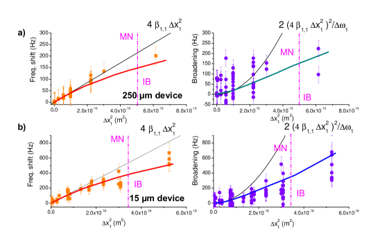
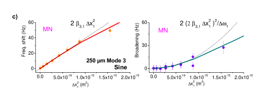
Refer to caption
Refer to caption
Figure 17: Characteristics for 15μ𝜇\leavevmode\nobreak\ \mum and 250μ𝜇\leavevmode\nobreak\ \mum. Same data as Fig. 3 of the paper, for 2 other devices (see tabular 1). a) “self-coupling” on 250μ𝜇\leavevmode\nobreak\ \mum device. b) “self-coupling” on 15μ𝜇\leavevmode\nobreak\ \mum device. c) “mode-coupling” on 250μ𝜇\leavevmode\nobreak\ \mum device. Note that home-made filter and setup characteristics were different, and had to be calibrated following the same procedure as for 300μ𝜇\leavevmode\nobreak\ \mum devices.

All data show the same behavior, which is driven simply by the product of the frequency fluctuation amplitude (ΣδωsubscriptΣ𝛿𝜔\Sigma_{\delta\omega}) with the fluctuation correlation time (1/Δωn1Δsubscript𝜔𝑛1/\Delta\omega_{n}, the position fluctuation’s correlation time being 2/Δωn2Δsubscript𝜔𝑛2/\Delta\omega_{n}): this is precisely the parameter αλsubscript𝛼𝜆\alpha_{\lambda} called “motional narrowing parameter” in Ref. [41].

If this parameter is small, we are in the “motional narrowing” limit: the fluctuations are too fast to resolve the full frequency distribution. As such, the function with which we have to convolve the linear response is not strictly speaking a distribution of frequency realization, since it is complex-valued. The result of the phase-diffusion process is actually to shift the resonance frequency (by the average of the frequency fluctuations, βm,nΔxn2proportional-toabsentsubscript𝛽𝑚𝑛Δsuperscriptsubscript𝑥𝑛2\propto\beta_{m,n}\Delta x_{n}^{2}) at first order. At second order, it slightly broadens the resonance line without changing its shape: the effect is thus (βm,nΔxn2)2proportional-toabsentsuperscriptsubscript𝛽𝑚𝑛Δsuperscriptsubscript𝑥𝑛22\propto(\beta_{m,n}\Delta x_{n}^{2})^{2}. The first term is simply the “dressing” of the mode by the interaction with all the others, while the second one is truly the “decoherence” effect; the first one is a certain quantity, while the second one quantifies by how much the frequency of the measured mode fluctuates.

If the motional narrowing parameter αλsubscript𝛼𝜆\alpha_{\lambda} is large, then we are in the “inhomogeneous broadening” limit. This is the case of Ref. [34] for instance. Note that with an artificial telegraph frequency noise generated by a gate electrode, in Ref. [32] Chan and co-workers could switch from one limit to the other not by tuning the amplitude of the noise, but its correlation time instead. In this limit, the full range of fluctuations is spanned by the oscillating mode, and one simply measures the averaged motion over all frequency realizations (assuming that the acquisition time is slow enough to capture all fluctuations) [50]. In this case, the resonance expressions can also be simply described by a convolution with ρλ(δω)subscript𝜌𝜆𝛿𝜔\rho_{\lambda}(\delta\omega), λ=n,m𝜆𝑛𝑚\lambda=n,m or n,m𝑛𝑚n,m:

SXn(ω)superscriptsubscript𝑆𝑋𝑛𝜔\displaystyle S_{X}^{n}(\omega) =\displaystyle= SLorentzn(ω)ρn(ω)Noise on n, measure noise on nsuperscriptsubscript𝑆𝐿𝑜𝑟𝑒𝑛𝑡𝑧𝑛𝜔subscript𝜌𝑛𝜔Noise on n, measure noise on n\displaystyle S_{Lorentz}^{n}(\omega)\ast\rho_{n}(\omega)\,\,\,\,\,\mbox{Noise on $n$, measure noise on $n$}
x~m0superscriptsubscript~𝑥𝑚0\displaystyle\tilde{x}_{m}^{0} =\displaystyle= XLorentzm(ω)ρm(ω)Noise on m, measure sine on msuperscriptsubscript𝑋𝐿𝑜𝑟𝑒𝑛𝑡𝑧𝑚𝜔subscript𝜌𝑚𝜔Noise on m, measure sine on m\displaystyle X_{Lorentz}^{m}(\omega)\ast\rho_{m}(\omega)\,\,\,\,\,\mbox{Noise on $m$, measure sine on $m$}
x~m0superscriptsubscript~𝑥𝑚0\displaystyle\tilde{x}_{m}^{0} =\displaystyle= XLorentzm(ω)ρm,n(ω)Noise on n, measure sine on m,superscriptsubscript𝑋𝐿𝑜𝑟𝑒𝑛𝑡𝑧𝑚𝜔subscript𝜌𝑚𝑛𝜔Noise on n, measure sine on m\displaystyle X_{Lorentz}^{m}(\omega)\ast\rho_{m,n}(\omega)\,\,\,\,\,\mbox{Noise on $n$, measure sine on $m$},

with ρλ(δω)subscript𝜌𝜆𝛿𝜔\rho_{\lambda}(\delta\omega) the frequency distributions directly obtained from ρ(δr)𝜌𝛿𝑟\rho(\delta r) the distribution of position amplitudes. They simply write:

ρ(δr)𝜌𝛿𝑟\displaystyle\rho(\delta r) =\displaystyle= 1Δxn2δrexp[12Δxn2δr2]Θ[δr],1Δsuperscriptsubscript𝑥𝑛2𝛿𝑟12Δsuperscriptsubscript𝑥𝑛2𝛿superscript𝑟2Θdelimited-[]𝛿𝑟\displaystyle\frac{1}{\Delta x_{n}^{2}}\delta r\exp\left[-\frac{1}{2\,\Delta x_{n}^{2}}\delta r^{2}\right]\,\Theta\left[\delta r\right],
ρn(δω)subscript𝜌𝑛𝛿𝜔\displaystyle\rho_{n}(\delta\omega) =\displaystyle= 1Σδωnexp(δωΣδωn),1superscriptsubscriptΣ𝛿𝜔𝑛𝛿𝜔superscriptsubscriptΣ𝛿𝜔𝑛\displaystyle\frac{1}{\Sigma_{\delta\omega}^{n}}\exp\left(-\frac{\delta\omega}{\Sigma_{\delta\omega}^{n}}\right),
ρm(δω)subscript𝜌𝑚𝛿𝜔\displaystyle\rho_{m}(\delta\omega) =\displaystyle= 1Σδωmexp(δωΣδωm),1superscriptsubscriptΣ𝛿𝜔𝑚𝛿𝜔superscriptsubscriptΣ𝛿𝜔𝑚\displaystyle\frac{1}{\Sigma_{\delta\omega}^{m}}\exp\left(-\frac{\delta\omega}{\Sigma_{\delta\omega}^{m}}\right),
ρm,n(δω)subscript𝜌𝑚𝑛𝛿𝜔\displaystyle\rho_{m,n}(\delta\omega) =\displaystyle= 1Σδωm,nexp(δωΣδωm,n),1superscriptsubscriptΣ𝛿𝜔𝑚𝑛𝛿𝜔superscriptsubscriptΣ𝛿𝜔𝑚𝑛\displaystyle\frac{1}{\Sigma_{\delta\omega}^{m,n}}\exp\left(-\frac{\delta\omega}{\Sigma_{\delta\omega}^{m,n}}\right),

with the standard deviations of the frequency noises defined by:

ΣδωnsuperscriptsubscriptΣ𝛿𝜔𝑛\displaystyle\Sigma_{\delta\omega}^{n} =\displaystyle= 2βn,nΔxn2,2subscript𝛽𝑛𝑛Δsuperscriptsubscript𝑥𝑛2\displaystyle 2\beta_{n,n}\Delta x_{n}^{2},
ΣδωmsuperscriptsubscriptΣ𝛿𝜔𝑚\displaystyle\Sigma_{\delta\omega}^{m} =\displaystyle= 4βm,mΔxn2,4subscript𝛽𝑚𝑚Δsuperscriptsubscript𝑥𝑛2\displaystyle 4\beta_{m,m}\Delta x_{n}^{2},
Σδωm,nsuperscriptsubscriptΣ𝛿𝜔𝑚𝑛\displaystyle\Sigma_{\delta\omega}^{m,n} =\displaystyle= 2βm,nΔxn2.2subscript𝛽𝑚𝑛Δsuperscriptsubscript𝑥𝑛2\displaystyle 2\beta_{m,n}\Delta x_{n}^{2}.

Above, Θ[x]Θdelimited-[]𝑥\Theta[x] is the Heaviside step function. The position distribution is a 2D-Gaussian, while the frequency distributions are exponentials; only the couplings are different in the above expressions, and in the paper we simply quote ΣδωsubscriptΣ𝛿𝜔\Sigma_{\delta\omega} without index.

The simple averaging procedure works well for large αλsubscript𝛼𝜆\alpha_{\lambda} [34]. However, even for moderate motional narrowing parameters it seems to reproduce not too badly the shapes measured (over estimating a bit the broadening); but it fails to capture the certain frequency shift, by construction. For very high Q𝑄Q and small noise levels, the resolution of the measurement can nonetheless be good enough to demonstrate the difference between the two approaches: this is shown in Fig. 18. Again, we demonstrate very good agreement with the exact theoretical calculation [41]: the “motional narrowing” effect reduces the impact of the asymmetry of the actual frequency-distribution.
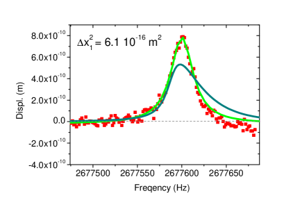
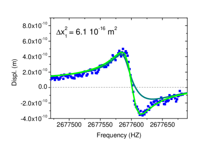
Refer to caption
Refer to caption
Figure 18: Comparing fits. Data taken on sample 250μ𝜇\leavevmode\nobreak\ \mum-n1, measuring mode m=3𝑚3m=3 while driving fluctuations on mode n=1𝑛1n=1 (X quadrature on the left, and Y on the right). The applied field is 1  T for a force F30=0.13superscriptsubscript𝐹300.13F_{3}^{0}=0.13\leavevmode\nobreak\ pN; the actual mode n=1𝑛1n=1 position fluctuations is quoted in inset. The full green line is the exact theoretical fit, while the dark grey corresponds to the simple average (“inhomogeneous broadening” theory, here peak shifted by about 15  Hz to match data, see text).

7 Measured correlators and noise spectra

The theory applied from Ref. [41] is valid for small sine wave excitations: one should remain in the linear response limit. In this limit, there should be no back-action of the sinusoidal drive onto the statistics of the fluctuations, even though their spectra can be altered.

So, from the experimental point of view, it is important to check that this limit is satisfied. We thus first show in Fig. 19 the raw spectra obtained with no sine wave excitation applied for both small and large noise amplitudes. We see that even if the spectrum is distorted at large Brownian motion levels, we still confirm that X and Y quadratures are equivalent; no cross correlations are detected either. The physical situation is perfectly normal, as it should be for a high Q𝑄Q device [45].

Refer to caption
Refer to caption
Figure 19: Raw spectra, no sine-wave drive. Raw spectra for mode n=1 measured for small (left, Δx12=2.2 1017Δsuperscriptsubscript𝑥12superscript2.21017\Delta x_{1}^{2}=2.2\,10^{-17}\leavevmode\nobreak\ m2) and large (right, Δx12=4. 1015Δsuperscriptsubscript𝑥12superscript4.1015\Delta x_{1}^{2}=4.\,10^{-15}\leavevmode\nobreak\ m2) noise levels, with no sine-wave drive. Data from sample 250μ𝜇\leavevmode\nobreak\ \mum-n1 taken at 1  T, with X quadrature in red, and Y in blue. The green inset is the cross-correlation spectrum. Acquisition bandwidth 787878\leavevmode\nobreak\ Hz.

But we expect new phenomena to show up if a strong sine-wave signal is applied, like e.g. noise squeezing [44]. In Fig. 20 we show raw spectra obtained with a rather strong sinusoidal force applied onto mode m=1𝑚1m=1 or m=3𝑚3m=3, compared to smaller ones (or none). Of course, the data presented in the main part of the paper are obtained with the smallest possible drive levels. What we see is that when mode m=3𝑚3m=3 is excited, the noise spectrum measured on n=1𝑛1n=1 simply shifts with the amplitude of the sine wave motion. This is nothing but the usual “mode-coupling” effect [39], but seen on a noise spectrum. From β1,3=4. 1016subscript𝛽13superscript4.1016\beta_{1,3}=4.\,10^{16}\leavevmode\nobreak\ Hz/m2, we compute a shift of the order of 300300300\leavevmode\nobreak\ Hz consistent with Fig. 20. No correlations between X and Y are detected, and the two spectra are equivalent.
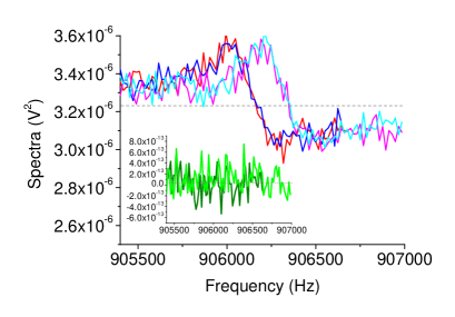
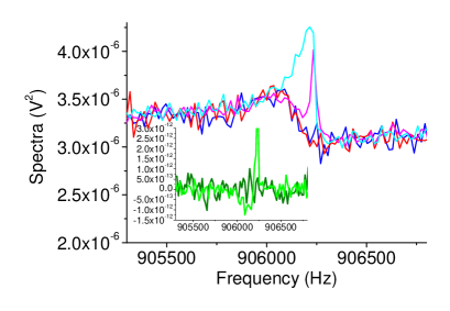
Refer to caption
Refer to caption
Figure 20: Raw spectra, with sine-wave drive. Raw spectra of Brownian motion of mode n=1𝑛1n=1 measured with a sinusoidal drive on the third mode m=3𝑚3m=3 (left), and on the first m=1𝑚1m=1 (right). Data from sample 250μ𝜇\leavevmode\nobreak\ \mum-n1 taken at 1  T, with X quadrature in red, and Y in blue. The green inset is the cross-correlation spectrum. The dark color lines are the references with small (or none) sine-wave drive, while the light color corresponds to the strongly driven case. F30=0superscriptsubscript𝐹300F_{3}^{0}=0\leavevmode\nobreak\ pN and F30=3.1superscriptsubscript𝐹303.1F_{3}^{0}=3.1\leavevmode\nobreak\ pN (left), and F10=2.7superscriptsubscript𝐹102.7F_{1}^{0}=2.7\leavevmode\nobreak\ pN, F10=11superscriptsubscript𝐹1011F_{1}^{0}=11\leavevmode\nobreak\ pN (right) for small and large settings respectively. For all graphs the motional noise level was Δx12=2.2 1017Δsuperscriptsubscript𝑥12superscript2.21017\Delta x_{1}^{2}=2.2\,10^{-17}\leavevmode\nobreak\ m2. Acquisition bandwidth 787878\leavevmode\nobreak\ Hz.

The situation becomes more interesting when one drives strongly with a sine-wave the same mode where the noise is. We see a peak appearing in the XY𝑋𝑌XY correlation, and now spectra measured on X and Y are clearly different. We interpret these features as signatures of noise squeezing, as measured in Ref. [44]. We illustrate empirically the effect of large sinusoidal excitation levels on the measured response in Fig. 4 of the paper. The amplitude of the detected mechanical peak lies below the calculation, as if the impact of frequency noise was stronger than expected. Both the usual Duffing non-linearity of the mode and the altered statistics are responsible for the apparent saturation of the peak height. A new and difficult theoretical work would be needed to further investigate this very interesting regime.

8 Extension to thermally induced Brownian noise

When the stochastic driving force is a real thermal bath, the system is always in the “motional narrowing” limit. In this case, the response is Lorentzian with a “dressed” frequency, and an additional “thermal decoherence”. These can be written at lowest order with the simple expansions, respectively, reproducing the results of Ref. [41]:

ωnsubscript𝜔𝑛\displaystyle\omega_{n} =\displaystyle= ωn0+4βn,nΔxn2+mn2βn,mΔxm2+m2barβn,mΔym2,superscriptsubscript𝜔𝑛04subscript𝛽𝑛𝑛Δsuperscriptsubscript𝑥𝑛2subscript𝑚𝑛2subscript𝛽𝑛𝑚Δsuperscriptsubscript𝑥𝑚2subscriptsuperscript𝑚2barsubscript𝛽𝑛superscript𝑚Δsuperscriptsubscript𝑦superscript𝑚2\displaystyle\omega_{n}^{0}+4\beta_{n,n}\Delta x_{n}^{2}+\sum_{m\neq n}2\beta_{n,m}\Delta x_{m}^{2}+\sum_{m^{\prime}}2\mathrm{bar}{\beta}_{n,m^{\prime}}\Delta y_{m^{\prime}}^{2},
ΔωnΔsubscript𝜔𝑛\displaystyle\Delta\omega_{n} =\displaystyle= Δωn0+2(4βn,nΔxn2)2Δωn0+mn2(2βn,mΔxm2)2Δωm0+m2(2barβn,mΔym2)2Δbarωm0.Δsuperscriptsubscript𝜔𝑛02superscript4subscript𝛽𝑛𝑛Δsuperscriptsubscript𝑥𝑛22Δsuperscriptsubscript𝜔𝑛0subscript𝑚𝑛2superscript2subscript𝛽𝑛𝑚Δsuperscriptsubscript𝑥𝑚22Δsuperscriptsubscript𝜔𝑚0subscriptsuperscript𝑚2superscript2barsubscript𝛽𝑛superscript𝑚Δsuperscriptsubscript𝑦superscript𝑚22Δbarsuperscriptsubscript𝜔superscript𝑚0\displaystyle\Delta\omega_{n}^{0}+2\frac{\left(4\beta_{n,n}\Delta x_{n}^{2}\right)^{2}}{\Delta\omega_{n}^{0}}+\sum_{m\neq n}2\frac{\left(2\beta_{n,m}\Delta x_{m}^{2}\right)^{2}}{\Delta\omega_{m}^{0}}+\sum_{m^{\prime}}2\frac{\left(2\mathrm{bar}{\beta}_{n,m^{\prime}}\Delta y_{m^{\prime}}^{2}\right)^{2}}{\Delta\mathrm{bar}{\omega}_{m^{\prime}}^{0}}.

These are Eqs. (4) and (5) of the main paper, on which the thermal bath discussion is based. The validity of these expansions has been experimentally verified in the present work for two modes only, Figs. 3 & 17. They can be extended in this simple way to many modes since the Brownian motion between nm𝑛𝑚n\neq m is uncorrelated. For the sake of completeness, we also added the sum over the other family of transverse modes (in y𝑦\vec{y} direction), which coefficients are designed with a bar, and the index with a prime (the position standard deviation simply writes Δym2Δsuperscriptsubscript𝑦superscript𝑚2\Delta y_{m^{\prime}}^{2}). The nonlinear coupling between flexural modes of different family has been studied recently [D. Cadeddu et al. Nano Letters 16, 926 (2016)]. The calculation of Section 5 is easily adapted with u(z,t)=xn(t)Ψn(z)+ym(t)barΨm(z)𝑢𝑧𝑡subscript𝑥𝑛𝑡subscriptΨ𝑛𝑧subscript𝑦superscript𝑚𝑡barsubscriptΨsuperscript𝑚𝑧u(z,t)=x_{n}(t)\Psi_{n}(z)+y_{m^{\prime}}(t)\mathrm{bar}{\Psi}_{m^{\prime}}(z). Note that the mode shapes (and mode numbers) can be a bit different along the x𝑥\vec{x}, y𝑦\vec{y} axes because the beam may not be a perfect square; the second moment of area Izsubscript𝐼𝑧I_{z} is a bit different for the two families. Hence the bar notation introduced above.

Using the integrals In,msubscript𝐼𝑛𝑚I_{n,m} over mode shapes introduced in Section 5, and the simple equipartition result Δxn2=kBT/knΔsuperscriptsubscript𝑥𝑛2subscript𝑘𝐵𝑇subscript𝑘𝑛\Delta x_{n}^{2}=k_{B}T/k_{n}, Δym2=kBT/barkmΔsuperscriptsubscript𝑦superscript𝑚2subscript𝑘𝐵𝑇barsubscript𝑘superscript𝑚\Delta y_{m^{\prime}}^{2}=k_{B}T/\mathrm{bar}{k}_{m^{\prime}} we can rewrite these expressions such that:

ωnωn0ωn0subscript𝜔𝑛superscriptsubscript𝜔𝑛0superscriptsubscript𝜔𝑛0\displaystyle\!\!\!\!\!\!\!\!\!\!\!\!\!\!\frac{\omega_{n}-\omega_{n}^{0}}{\omega_{n}^{0}} =\displaystyle\!\!\!\!\!\!= (EbeamA2L3)(kBT)(2kn2)[m(In,nIm,m+2In,m2)(km/kn)+m(In,nbarIm,m+2I~n,m2)(barkm/kn)],subscript𝐸𝑏𝑒𝑎𝑚𝐴2superscript𝐿3subscript𝑘𝐵𝑇2superscriptsubscript𝑘𝑛2delimited-[]subscript𝑚subscript𝐼𝑛𝑛subscript𝐼𝑚𝑚2superscriptsubscript𝐼𝑛𝑚2subscript𝑘𝑚subscript𝑘𝑛subscriptsuperscript𝑚subscript𝐼𝑛𝑛barsubscript𝐼superscript𝑚superscript𝑚2superscriptsubscript~𝐼𝑛superscript𝑚2barsubscript𝑘superscript𝑚subscript𝑘𝑛\displaystyle\!\!\!\!\!\!\left(\frac{E_{beam}A}{2L^{3}}\right)\frac{(k_{B}T)}{(2k_{n}^{2})}\left[\sum_{m}\frac{(I_{n,n}I_{m,m}+2I_{n,m}^{2})}{(k_{m}/k_{n})}+\sum_{m^{\prime}}\frac{(I_{n,n}\mathrm{bar}{I}_{m^{\prime},m^{\prime}}+2\tilde{I}_{n,m^{\prime}}^{2})}{(\mathrm{bar}{k}_{m^{\prime}}/k_{n})}\right]\!\!, (23)
ΔωnΔωn0Δωn0Δsubscript𝜔𝑛Δsuperscriptsubscript𝜔𝑛0Δsuperscriptsubscript𝜔𝑛0\displaystyle\!\!\!\!\!\!\!\!\!\!\!\!\!\!\!\!\!\frac{\Delta\omega_{n}-\Delta\omega_{n}^{0}}{\Delta\omega_{n}^{0}} =\displaystyle\!\!\!\!\!\!\!= (EbeamA2L3)2(kBT)2(2kn4)Qn2[mQmQn(In,nIm,m+2In,m2)2(km/kn)2(ωm0/ωn0)+mbarQmQn(In,nbarIm,m+2I~n,m2)2(barkm/kn)2(barωm0/ωn0)],superscriptsubscript𝐸𝑏𝑒𝑎𝑚𝐴2superscript𝐿32superscriptsubscript𝑘𝐵𝑇22superscriptsubscript𝑘𝑛4superscriptsubscript𝑄𝑛2delimited-[]subscript𝑚subscript𝑄𝑚subscript𝑄𝑛superscriptsubscript𝐼𝑛𝑛subscript𝐼𝑚𝑚2superscriptsubscript𝐼𝑛𝑚22superscriptsubscript𝑘𝑚subscript𝑘𝑛2superscriptsubscript𝜔𝑚0superscriptsubscript𝜔𝑛0subscriptsuperscript𝑚barsubscript𝑄superscript𝑚subscript𝑄𝑛superscriptsubscript𝐼𝑛𝑛barsubscript𝐼superscript𝑚superscript𝑚2superscriptsubscript~𝐼𝑛superscript𝑚22superscriptbarsubscript𝑘superscript𝑚subscript𝑘𝑛2barsuperscriptsubscript𝜔superscript𝑚0superscriptsubscript𝜔𝑛0\displaystyle\!\!\!\!\!\!\!\left(\frac{E_{beam}A}{2L^{3}}\right)^{2}\frac{(k_{B}T)^{2}}{(2k_{n}^{4})}Q_{n}^{2}\left[\sum_{m}\frac{Q_{m}}{Q_{n}}\frac{(I_{n,n}I_{m,m}+2I_{n,m}^{2})^{2}}{(k_{m}/k_{n})^{2}(\omega_{m}^{0}/\omega_{n}^{0})}+\sum_{m^{\prime}}\frac{\mathrm{bar}{Q}_{m^{\prime}}}{Q_{n}}\frac{(I_{n,n}\mathrm{bar}{I}_{m^{\prime},m^{\prime}}+2\tilde{I}_{n,m^{\prime}}^{2})^{2}}{(\mathrm{bar}{k}_{m^{\prime}}/k_{n})^{2}(\mathrm{bar}{\omega}_{m^{\prime}}^{0}/\omega_{n}^{0})}\right]\!\!, (24)

having introduced equivalent integrals with bar and tilde applying to the other mode family (and cross term):

In,msubscript𝐼𝑛𝑚\displaystyle I_{n,m} =\displaystyle= L0LΨn(z)Ψm(z)𝑑z,𝐿subscriptsuperscript𝐿0subscriptΨ𝑛superscript𝑧subscriptΨ𝑚superscript𝑧differential-d𝑧\displaystyle L\int^{L}_{0}\Psi_{n}(z)^{{}^{\prime}}\Psi_{m}(z)^{{}^{\prime}}dz,
barIn,mbarsubscript𝐼superscript𝑛superscript𝑚\displaystyle\mathrm{bar}{I}_{n^{\prime},m^{\prime}} =\displaystyle= L0LbarΨn(z)barΨm(z)𝑑z,𝐿subscriptsuperscript𝐿0barsubscriptΨsuperscript𝑛superscript𝑧barsubscriptΨsuperscript𝑚superscript𝑧differential-d𝑧\displaystyle L\int^{L}_{0}\mathrm{bar}{\Psi}_{n^{\prime}}(z)^{{}^{\prime}}\mathrm{bar}{\Psi}_{m^{\prime}}(z)^{{}^{\prime}}dz,
I~n,msubscript~𝐼𝑛superscript𝑚\displaystyle\tilde{I}_{n,m^{\prime}} =\displaystyle= L0LΨn(z)barΨm(z)𝑑z.𝐿subscriptsuperscript𝐿0subscriptΨ𝑛superscript𝑧barsubscriptΨsuperscript𝑚superscript𝑧differential-d𝑧\displaystyle L\int^{L}_{0}\Psi_{n}(z)^{{}^{\prime}}\mathrm{bar}{\Psi}_{m^{\prime}}(z)^{{}^{\prime}}dz.

The terms in brackets in Eqs. (23-24) have no dimensions and can be calculated from mode parameters. This is what we describe below. The prefactor gives the strength of the effect from materials properties and geometry.

Up to date, there is no universal microscopic model explaining nano-mechanical damping, even though many theories exist. They are however phenomenological descriptions of experimental results on SiN beams, e.g. Quirin P. Unterreithmeier et al., PRL 105, 027205 (2010) and A. Suhel et al. APL 100, 173111 (2012). For our devices, we have verified that these approaches apply rather well, see M. Defoort, PhD thesis Université de Grenoble (2014). To make our estimates of “thermal decoherence”, we thus use the lowest order expression representing a damping proportional to the bending energy Qn(Ebending+Etension)/Ebendingproportional-tosubscript𝑄𝑛subscript𝐸𝑏𝑒𝑛𝑑𝑖𝑛𝑔subscript𝐸𝑡𝑒𝑛𝑠𝑖𝑜𝑛subscript𝐸𝑏𝑒𝑛𝑑𝑖𝑛𝑔Q_{n}\propto(E_{bending}+E_{tension})/E_{bending}. The formulas are summarized in Tab. 2, computed from the mode shapes Ψn(z)subscriptΨ𝑛𝑧\Psi_{n}(z) in the two limits of interest: low-stress and high-stress (see discussion below). While these expressions of Qnsubscript𝑄𝑛Q_{n} are clearly not enough to fit perfectly the experimental findings (it overestimates the Q𝑄Qs at high n𝑛n), it is a good starting point since it does not involve any fit parameter in the computation of the bracket of Eq. (24), and leads to the proper tendency for the sums involved. This will at least produce a very reasonable upper bound for our estimates.

The resonance frequencies verify (ωn0)2=kn/mnsuperscriptsuperscriptsubscript𝜔𝑛02subscript𝑘𝑛subscript𝑚𝑛(\omega_{n}^{0})^{2}=k_{n}/m_{n}, and both knsubscript𝑘𝑛k_{n} and mnsubscript𝑚𝑛m_{n} can be readily computed from the mode shapes Ψn(z)subscriptΨ𝑛𝑧\Psi_{n}(z). The mass writes mn=ρbeamA0LΨn(z)2𝑑zsubscript𝑚𝑛subscript𝜌𝑏𝑒𝑎𝑚𝐴subscriptsuperscript𝐿0subscriptΨ𝑛superscript𝑧2differential-d𝑧m_{n}=\rho_{beam}A\int^{L}_{0}\Psi_{n}(z)^{2}dz, and the spring constant kn=EbeamIz0L(2Ψn[z]/z2)2𝑑z+T00L(2Ψn[z]/z2)Ψn(z)𝑑zsubscript𝑘𝑛subscript𝐸𝑏𝑒𝑎𝑚subscript𝐼𝑧subscriptsuperscript𝐿0superscriptsuperscript2subscriptΨ𝑛delimited-[]𝑧superscript𝑧22differential-d𝑧subscript𝑇0subscriptsuperscript𝐿0superscript2subscriptΨ𝑛delimited-[]𝑧superscript𝑧2subscriptΨ𝑛𝑧differential-d𝑧k_{n}=E_{beam}I_{z}\int^{L}_{0}(\partial^{2}\Psi_{n}[z]/\partial z^{2})^{2}dz+T_{0}\int^{L}_{0}(\partial^{2}\Psi_{n}[z]/\partial z^{2})\Psi_{n}(z)dz (first term stands for bending energy, second for tensioning; the same integrals are used for the estimate of the Q𝑄Qs). We limit the discussion to perfectly clamped beams. The mode shapes Ψn(z)subscriptΨ𝑛𝑧\Psi_{n}(z) (and barΨn[z]barsubscriptΨ𝑛delimited-[]𝑧\mathrm{bar}{\Psi}_{n}[z]) are then obtained by solving the (linear) Euler-Bernoulli equation.
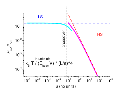
Refer to caption
Figure 21: Thermal frequency “dressing” coefficient vs in-built stress. Calculated sum in the bracket of Eq. (23) for a single family of modes. Here, numerics corresponding to mode n=1𝑛1n=1. The overall prefactor is given in inset (same definitions as for Fig. 22). The two limits are depicted (low-stress LS and high-stress HS), with their asymptotic behaviors (dashed lines).

A full analytical solution of the Euler-Bernoulli equation does not exist. However, two limiting cases can be described: low-stress u1much-less-than𝑢1u\ll 1 and high-stress u~1much-less-than~𝑢1\tilde{u}\ll 1 where we define u=T0L2/(EbeamIz)𝑢subscript𝑇0superscript𝐿2subscript𝐸𝑏𝑒𝑎𝑚subscript𝐼𝑧u=T_{0}L^{2}/(E_{beam}I_{z}) and u~=EbeamIz/(|T0|L2)~𝑢subscript𝐸𝑏𝑒𝑎𝑚subscript𝐼𝑧subscript𝑇0superscript𝐿2\tilde{u}=E_{beam}I_{z}/(\left|T_{0}\right|L^{2}). Our definitions are u<0𝑢0u<0 for tensile, and u~>0~𝑢0\tilde{u}>0. In these regimes, analytic shapes can be found as Taylor expansions of u𝑢u (and u~~𝑢\sqrt{\tilde{u}}), and integrated to obtain all the required parameters. We summarize the results in Tabs. 3 and 4 respectively (and Tab. 2 for Q𝑄Q factors). In the low-stress case, we fit analytic functions that reproduce rather well the numerical results, and have the proper asymptotic dependence for large n𝑛n. For high-stress, the expansion is exact at the lowest orders in u~~𝑢\tilde{u}. This is the limit that applies to all our SiN beams. Note that if all modes would be perfectly orthogonal, the In,msubscript𝐼𝑛𝑚I_{n,m} terms would be 0 for nm𝑛𝑚n\neq m (and barIn,mbarsubscript𝐼superscript𝑛superscript𝑚\mathrm{bar}{I}_{n^{\prime},m^{\prime}}, I~n,msubscript~𝐼𝑛superscript𝑚\tilde{I}_{n,m^{\prime}} as well). This is not strictly the case, as shown in Tab. 5.

n𝑛n 𝒬n0superscriptsubscript𝒬𝑛0{\cal Q}_{n}^{0} 𝒬n1superscriptsubscript𝒬𝑛1{\cal Q}_{n}^{1} 𝒬n0superscriptsubscript𝒬𝑛0{\cal Q}_{n}^{0} 𝒬n1superscriptsubscript𝒬𝑛1{\cal Q}_{n}^{1} 𝒬n2superscriptsubscript𝒬𝑛2{\cal Q}_{n}^{2}
1 111 0.030270.03027-0.03027\cdots 111 222 17.87017.87017.870\cdots
2 111 0.0150.015-0.015\cdots 111 222 47.48047.48047.480\cdots
3 111 0.007600.00760-0.00760\cdots \cdots \cdots \cdots
4 111 0.00450.0045-0.0045\cdots \cdots \cdots \cdots
5 111 0.003000.00300-0.00300\cdots \cdots \cdots \cdots
\cdots \cdots \cdots \cdots \cdots \cdots
n𝑛n 111 0.0161+0.0322n+0.101n2n3(n+2.2)0.01610.0322𝑛0.101superscript𝑛2superscript𝑛3𝑛2.2-\frac{0.0161\cdots+0.0322\cdots n+0.101\cdots n^{2}}{n^{3}(n+2.2)} 111 2 2[4+(nπ)22]2delimited-[]4superscript𝑛𝜋222\left[4+\frac{(n\pi)^{2}}{2}\right]
±plus-or-minus\pm1  % n4𝑛4n\geq 4
Table 2: Numerical results for estimates of Q𝑄Q factors of low-stress beams (left, Qn=Q0×[𝒬n0+u𝒬n1]subscript𝑄𝑛subscript𝑄0delimited-[]superscriptsubscript𝒬𝑛0𝑢superscriptsubscript𝒬𝑛1Q_{n}=Q_{0}\times[{\cal Q}_{n}^{0}+u\,{\cal Q}_{n}^{1}]) and high-stress beams (right, Qn=Q0×[𝒬n0+u~𝒬n1+u~𝒬n2]/[u~𝒬n1+u~𝒬n2]subscript𝑄𝑛subscript𝑄0delimited-[]superscriptsubscript𝒬𝑛0~𝑢superscriptsubscript𝒬𝑛1~𝑢superscriptsubscript𝒬𝑛2delimited-[]~𝑢superscriptsubscript𝒬𝑛1~𝑢superscriptsubscript𝒬𝑛2Q_{n}=Q_{0}\times[{\cal Q}_{n}^{0}+\sqrt{\tilde{u}}\,{\cal Q}_{n}^{1}+\tilde{u}\,{\cal Q}_{n}^{2}]/[\sqrt{\tilde{u}}\,{\cal Q}_{n}^{1}+\tilde{u}\,{\cal Q}_{n}^{2}]), assuming losses proportional to bending energy (see text). Tensile means u<0𝑢0u<0, and u~>0~𝑢0\tilde{u}>0 by construction. Q0subscript𝑄0Q_{0} is a fit parameter corresponding to the bending-limited Q𝑄Q factor. Expansions are exact for high-stress, and the fit error to numerics is specified for low-stress.

In Figs. 21 and 22 we show the u𝑢u-dependence of the brackets in Eqs. (23-24) calculated from the Tabulars for mode n=1𝑛1n=1 (first flexure). We compute only a single sum, the one on the same family of modes; for a perfectly squared (monolithic) beam, taking into account the second sum simply amounts to multiply the result by 2. In the more generic case of a bilayer and rectangular beam, the barIn,mbarsubscript𝐼superscript𝑛superscript𝑚\mathrm{bar}{I}_{n^{\prime},m^{\prime}}, I~n,msubscript~𝐼𝑛superscript𝑚\tilde{I}_{n,m^{\prime}} should be computed correctly. Thanks to the denominator in the sums, they converge reasonably quickly (much before the high-frequency cut-off that should delimit the validity range of the Euler-Bernoulli equation; namely the atomic size for the wavelength associated to high-frequency modes or the phonon correlation time, whichever comes first).
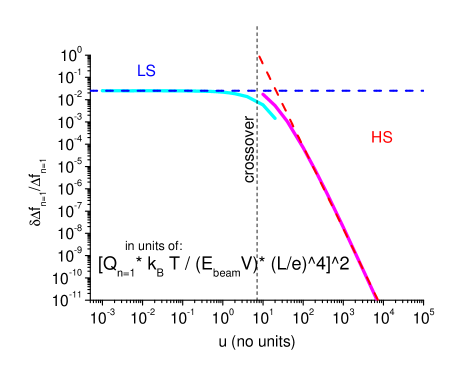
Refer to caption
Figure 22: Thermal “dephasing” coefficient vs in-built stress. Calculated sum in the bracket of Eq. (24) for a single family of modes. Here, numerics corresponding to mode n=1𝑛1n=1. The overall prefactor is given in inset (see text). The two limits are depicted (low-stress LS and high-stress HS), with their asymptotic behaviors (dashed lines).

The exact numerical values obtained in Figs. 21 and 22 are of order 0.1absent0.1\approx 0.1 for low-stress, but fall very quickly with increasing stress. Clearly, only for low-stress devices shall this effect be relevant. The “dressing” of the resonance frequency is a certain value if T𝑇T is fixed; any temperature instability will translate into a frequency noise which can be calculated from Fig. 21. Furthermore, the strength of “thermal decoherence” for low-stress devices is essentially given by the prefactor (EbeamA2L3)2(kBT)2(2kn4)Qn2superscriptsubscript𝐸𝑏𝑒𝑎𝑚𝐴2superscript𝐿32superscriptsubscript𝑘𝐵𝑇22superscriptsubscript𝑘𝑛4superscriptsubscript𝑄𝑛2\left(\frac{E_{beam}A}{2L^{3}}\right)^{2}\frac{(k_{B}T)^{2}}{(2k_{n}^{4})}Q_{n}^{2}. It goes quadratically with temperature, and since knEbeam(we3/L3)proportional-tosubscript𝑘𝑛subscript𝐸𝑏𝑒𝑎𝑚𝑤superscript𝑒3superscript𝐿3k_{n}\propto E_{beam}(we^{3}/L^{3}) it depends very strongly on the aspect ratio e/L𝑒𝐿e/L of the structure (see inset of Fig. 22, (kBT)2Qn2/(EbeamV)2×(L/e)8proportional-toabsentsuperscriptsubscript𝑘𝐵𝑇2superscriptsubscript𝑄𝑛2superscriptsubscript𝐸𝑏𝑒𝑎𝑚𝑉2superscript𝐿𝑒8\propto(k_{B}T)^{2}Q_{n}^{2}/(E_{beam}V)^{2}\times(L/e)^{8} with V=weL𝑉𝑤𝑒𝐿V=weL the volume of the beam). It becomes obvious that low-stress bottom-up structures, especially with high-Q𝑄Q, shall be very sensitive to this effect. In practice, it means that an unstressed doubly-clamped nanotube can display a poor spectral Q𝑄Q even if its intrinsic one is high, limiting thus sensing applications. A conclusion also reached by different means in Ref. [30].

n𝑛n n0superscriptsubscript𝑛0{\cal L}_{n}^{0} n1superscriptsubscript𝑛1{\cal L}_{n}^{1} 𝒦n0superscriptsubscript𝒦𝑛0{\cal K}_{n}^{0} 𝒦n1superscriptsubscript𝒦𝑛1{\cal K}_{n}^{1} n0superscriptsubscript𝑛0{\cal M}_{n}^{0} n1superscriptsubscript𝑛1{\cal M}_{n}^{1} n0superscriptsubscript𝑛0{\cal I}_{n}^{0} n1superscriptsubscript𝑛1{\cal I}_{n}^{1}
1 4.730044.730044.73004\cdots 0.029060.02906-0.02906\cdots 198.46198.46198.46\cdots 5.094945.09494-5.09494\cdots 0.3964780.3964780.396478\cdots 0.00043400.0004340-0.0004340\cdots 4.87774.87774.8777\cdots 0.00063610.00063610.0006361\cdots
2 7.853207.853207.85320\cdots 0.023770.02377-0.02377\cdots 1 669.91669.91\,669.9\cdots 20.217320.2173-20.2173\cdots 0.4390280.4390280.439028\cdots 0.00011600.0001160-0.0001160\cdots 20.21720.21720.217\cdots 0.0034490.0034490.003449\cdots
3 10.995610.995610.9956\cdots 0.018600.01860-0.01860\cdots 7 394.57394.57\,394.5\cdots 42.499742.4997-42.4997\cdots 0.5058600.5058600.505860\cdots 0.000515280.000515280.00051528\cdots 50.03250.03250.032\cdots 0.055010.055010.05501\cdots
4 14.137214.137214.1372\cdots 0.0151820.015182-0.015182\cdots 20 082.820082.820\,082.8\cdots 77.671377.6713-77.6713\cdots 0.5027770.5027770.502777\cdots 0.000215250.000215250.00021525\cdots 86.27086.27086.270\cdots 0.039450.039450.03945\cdots
5 17.278817.278817.2788\cdots 0.0127940.012794-0.012794\cdots 44 545.444545.444\,545.4\cdots 123.614123.614-123.614\cdots 0.4997500.4997500.499750\cdots 0.000093260.000093260.00009326\cdots 131.93131.93131.93\cdots 0.027260.027260.02726\cdots
6 20.420320.420320.4203\cdots 0.011040.01104-0.01104\cdots 86 919.886919.886\,919.8\cdots 178.034178.034-178.034\cdots 0.4998800.4998800.499880\cdots 0.000057480.000057480.00005748\cdots 189.12189.12189.12\cdots 0.022820.022820.02282\cdots
7 23.561923.561923.5619\cdots 0.009710.00971-0.00971\cdots 154 107.5154107.5154\,107.5\cdots 242.210242.210-242.210\cdots 0.5000110.5000110.500011\cdots 0.000038340.000038340.00003834\cdots 254.02254.02254.02\cdots 0.020320.020320.02032\cdots
\cdots \cdots \cdots \cdots \cdots \cdots \cdots \cdots \cdots
n𝑛n nπ[1+12n]𝑛𝜋delimited-[]112𝑛n\pi\left[1+\frac{1}{2n}\right] 14πn[11n]14𝜋𝑛delimited-[]11𝑛-\frac{1}{4\pi n}\left[1-\frac{1}{n}\right] (nπ)42[1+2.2n]superscript𝑛𝜋42delimited-[]12.2𝑛\frac{(n\pi)^{4}}{2}\left[1+\frac{2.2\cdots}{n}\right] (nπ)22superscript𝑛𝜋22-\frac{(n\pi)^{2}}{2} 1212\frac{1}{2} 00 (n+12)2π22(n+12)π2superscript𝑛122superscript𝜋22𝑛12𝜋2\frac{(n+\frac{1}{2})^{2}\pi^{2}-2(n+\frac{1}{2})\pi}{2} 12(n+12)π1(n+12)2π212𝑛12𝜋1superscript𝑛122superscript𝜋2\frac{1}{2}\frac{(n+\frac{1}{2})\pi-1}{(n+\frac{1}{2})^{2}\pi^{2}}
±plus-or-minus\pm0.5  % n1𝑛1n\geq 1 ±plus-or-minus\pm1  % n5𝑛5n\geq 5 ±plus-or-minus\pm1.6  % n5𝑛5n\geq 5 ±plus-or-minus\pm1  % n1𝑛1n\geq 1 ±plus-or-minus\pm0.6  % n4𝑛4n\geq 4 Negligible ±plus-or-minus\pm1  % n3𝑛3n\geq 3 ±plus-or-minus\pm2  % n5𝑛5n\geq 5
Table 3: Numerical results for low-stress beams (see text). The coefficients listed stand for ωn0=(n0+un1)2EbeamIz/L3/(ρbeamAL)superscriptsubscript𝜔𝑛0superscriptsuperscriptsubscript𝑛0𝑢superscriptsubscript𝑛12subscript𝐸𝑏𝑒𝑎𝑚subscript𝐼𝑧superscript𝐿3subscript𝜌𝑏𝑒𝑎𝑚𝐴𝐿\omega_{n}^{0}=({\cal L}_{n}^{0}+u\,{\cal L}_{n}^{1})^{2}\sqrt{E_{beam}I_{z}/L^{3}/(\rho_{beam}AL)}, kn=(EbeamIz/L3)(𝒦n0+u𝒦n1)subscript𝑘𝑛subscript𝐸𝑏𝑒𝑎𝑚subscript𝐼𝑧superscript𝐿3superscriptsubscript𝒦𝑛0𝑢superscriptsubscript𝒦𝑛1k_{n}=(E_{beam}I_{z}/L^{3})({\cal K}_{n}^{0}+u\,{\cal K}_{n}^{1}), mn=(ρbeamAL)(n0+un1)subscript𝑚𝑛subscript𝜌𝑏𝑒𝑎𝑚𝐴𝐿superscriptsubscript𝑛0𝑢superscriptsubscript𝑛1m_{n}=(\rho_{beam}AL)({\cal M}_{n}^{0}+u\,{\cal M}_{n}^{1}), and In,n=n0+un1subscript𝐼𝑛𝑛superscriptsubscript𝑛0𝑢superscriptsubscript𝑛1I_{n,n}={\cal I}_{n}^{0}+u\,{\cal I}_{n}^{1}. We remind that our definition of motion amplitude xnsubscript𝑥𝑛x_{n} is the maximum value along the beam; and tensile means u<0𝑢0u<0. We give fits to these coefficients as a function of n𝑛n, with the stated accuracy in the last line.
n𝑛n n0superscriptsubscript𝑛0{\cal L}_{n}^{0} n1superscriptsubscript𝑛1{\cal L}_{n}^{1} n2superscriptsubscript𝑛2{\cal L}_{n}^{2} 𝒦n0superscriptsubscript𝒦𝑛0{\cal K}_{n}^{0} 𝒦n1superscriptsubscript𝒦𝑛1{\cal K}_{n}^{1} 𝒦n2superscriptsubscript𝒦𝑛2{\cal K}_{n}^{2} n0superscriptsubscript𝑛0{\cal M}_{n}^{0} n1superscriptsubscript𝑛1{\cal M}_{n}^{1} n2superscriptsubscript𝑛2{\cal M}_{n}^{2} n0superscriptsubscript𝑛0{\cal I}_{n}^{0} n1superscriptsubscript𝑛1{\cal I}_{n}^{1} n2superscriptsubscript𝑛2{\cal I}_{n}^{2}
1 1.77241.77241.7724\cdots 1.77241.77241.7724\cdots 7.03207.03207.0320\cdots 4.93484.93484.9348\cdots 9.86969.86969.8696\cdots 68.443768.443768.4437\cdots 0.50.50.5 11-1 00 4.93484.93484.9348\cdots 00 19.73919.739-19.739\cdots
\cdots \cdots \cdots \cdots \cdots \cdots \cdots \cdots \cdots \cdots \cdots \cdots \cdots
n𝑛n nπ𝑛𝜋\sqrt{n\pi} nπ𝑛𝜋\sqrt{n\pi} nπ[6+(nπ)24]𝑛𝜋delimited-[]6superscript𝑛𝜋24\sqrt{n\pi}\left[\frac{6+(n\pi)^{2}}{4}\right] (nπ)22superscript𝑛𝜋22\frac{(n\pi)^{2}}{2} (nπ)2superscript𝑛𝜋2(n\pi)^{2} 2(nπ)2+(nπ)422superscript𝑛𝜋2superscript𝑛𝜋422(n\pi)^{2}+\frac{(n\pi)^{4}}{2} 1212\frac{1}{2} 11-1 00 (nπ)22superscript𝑛𝜋22\frac{(n\pi)^{2}}{2} 0 2(nπ)22superscript𝑛𝜋2-2(n\pi)^{2}
Table 4: Numerical results for high-stress beams (see text). The coefficients listed stand for ωn0=(n0+u~n1+u~n2)2|T0|/L/(ρbeamAL)superscriptsubscript𝜔𝑛0superscriptsuperscriptsubscript𝑛0~𝑢superscriptsubscript𝑛1~𝑢superscriptsubscript𝑛22subscript𝑇0𝐿subscript𝜌𝑏𝑒𝑎𝑚𝐴𝐿\omega_{n}^{0}=({\cal L}_{n}^{0}+\sqrt{\tilde{u}}\,{\cal L}_{n}^{1}+\tilde{u}\,{\cal L}_{n}^{2})^{2}\sqrt{\left|T_{0}\right|/L/(\rho_{beam}AL)}, kn=(|T0|/L)(𝒦n0+u~𝒦n1+u~𝒦n2)subscript𝑘𝑛subscript𝑇0𝐿superscriptsubscript𝒦𝑛0~𝑢superscriptsubscript𝒦𝑛1~𝑢superscriptsubscript𝒦𝑛2k_{n}=(\left|T_{0}\right|/L)({\cal K}_{n}^{0}+\sqrt{\tilde{u}}\,{\cal K}_{n}^{1}+\tilde{u}\,{\cal K}_{n}^{2}), mn=(ρbeamAL)(n0+u~n1+u~n2)subscript𝑚𝑛subscript𝜌𝑏𝑒𝑎𝑚𝐴𝐿superscriptsubscript𝑛0~𝑢superscriptsubscript𝑛1~𝑢superscriptsubscript𝑛2m_{n}=(\rho_{beam}AL)({\cal M}_{n}^{0}+\sqrt{\tilde{u}}\,{\cal M}_{n}^{1}+\tilde{u}\,{\cal M}_{n}^{2}), and In,n=n0+u~n1+u~n2subscript𝐼𝑛𝑛superscriptsubscript𝑛0~𝑢superscriptsubscript𝑛1~𝑢superscriptsubscript𝑛2I_{n,n}={\cal I}_{n}^{0}+\sqrt{\tilde{u}}\,{\cal I}_{n}^{1}+\tilde{u}\,{\cal I}_{n}^{2}. We remind that our definition of motion amplitude xnsubscript𝑥𝑛x_{n} is the maximum value along the beam; and u~>0~𝑢0\tilde{u}>0 by construction. These expansions are exact.
n,m𝑛𝑚n,m n,m0superscriptsubscript𝑛𝑚0{\cal I}_{n,m}^{0} n,m1superscriptsubscript𝑛𝑚1{\cal I}_{n,m}^{1} n,m1superscriptsubscript𝑛𝑚1{\cal I}_{n,m}^{1} n,m2superscriptsubscript𝑛𝑚2{\cal I}_{n,m}^{2}
1,2 00 00 00 00
1,3 4.357864.357864.35786\cdots 0.0461080.0461080.046108\cdots 29.608829.608829.6088\cdots 118.435118.435118.435\cdots
1,4 00 00 \cdots \cdots
1,5 3.389853.38985-3.38985\cdots 0.0178250.017825-0.017825\cdots \cdots \cdots
1,6 00 00 \cdots \cdots
1,7 2.719582.719582.71958\cdots 0.00794370.00794370.0079437\cdots \cdots \cdots
1,8 00 00 \cdots \cdots
1,9 2.25582.2558-2.2558\cdots 0.003740.00374-0.00374\cdots \cdots \cdots
\cdots \cdots \cdots \cdots \cdots
2,3 00 00 00 00
2,4 8.047558.047558.04755\cdots 0.024380.024380.02438\cdots 78.95778.95778.957\cdots 315.83315.83315.83\cdots
2,5 00 00 \cdots \cdots
2,6 7.118167.11816-7.11816\cdots 0.0059670.005967-0.005967\cdots \cdots \cdots
\cdots \cdots \cdots \cdots \cdots
3,4 00 00 00 00
3,5 12.24312.24312.243\cdots 0.03220.03220.0322\cdots \cdots \cdots
3,6 00 00 \cdots \cdots
3,7 11.559411.5594-11.5594\cdots 0.016510.01651-0.01651\cdots \cdots \cdots
\cdots \cdots \cdots \cdots \cdots
4,5 00 00 00 00
4,6 15.679715.679715.6797\cdots Negligible \cdots \cdots
4,7 00 00 \cdots \cdots
4,8 15.331815.3318-15.3318\cdots Negligible \cdots \cdots
\cdots \cdots \cdots \cdots \cdots
n,m𝑛𝑚n,m 8π(n+12)2(m+12)2(n+m+1)[(n+m+1)2+(nm)2]×-\frac{8\pi(n+\frac{1}{2})^{2}(m+\frac{1}{2})^{2}}{(n+m+1)[(n+m+1)^{2}+(n-m)^{2}]}\times 00 nmπ2×-nm\pi^{2}\times 4nmπ2×-4nm\pi^{2}\times
(1+(1)n+m)2(1)C[(n1)2](1)C[(m1)2]1superscript1𝑛𝑚2superscript1𝐶delimited-[]𝑛12superscript1𝐶delimited-[]𝑚12\frac{(1+(-1)^{n+m})}{2}(-1)^{C[\frac{(n-1)}{2}]}(-1)^{C[\frac{(m-1)}{2}]} (1+(1)n+m)2(1)C[(n1)2](1)C[(m1)2]1superscript1𝑛𝑚2superscript1𝐶delimited-[]𝑛12superscript1𝐶delimited-[]𝑚12\frac{(1+(-1)^{n+m})}{2}(-1)^{C[\frac{(n-1)}{2}]}(-1)^{C[\frac{(m-1)}{2}]} (1+(1)n+m)2(1)C[(n1)2](1)C[(m1)2]1superscript1𝑛𝑚2superscript1𝐶delimited-[]𝑛12superscript1𝐶delimited-[]𝑚12\frac{(1+(-1)^{n+m})}{2}(-1)^{C[\frac{(n-1)}{2}]}(-1)^{C[\frac{(m-1)}{2}]}
±plus-or-minus\pm11  % n=1,m9formulae-sequence𝑛1𝑚9n=1,m\geq 9 Negligible
±plus-or-minus\pm6  % n2,m>2formulae-sequence𝑛2𝑚2n\geq 2,m>2
Table 5: Numerical results for cross term In,msubscript𝐼𝑛𝑚I_{n,m} (nm𝑛𝑚n\neq m) for low-stress beams (n,m0+un,m1superscriptsubscript𝑛𝑚0𝑢superscriptsubscript𝑛𝑚1{\cal I}_{n,m}^{0}+u\,{\cal I}_{n,m}^{1}, left) and high-stress beams (u~n,m1+u~n,m2~𝑢superscriptsubscript𝑛𝑚1~𝑢superscriptsubscript𝑛𝑚2\sqrt{\tilde{u}}\,{\cal I}_{n,m}^{1}+\tilde{u}\,{\cal I}_{n,m}^{2}, right). Note that In,m=Im,nsubscript𝐼𝑛𝑚subscript𝐼𝑚𝑛I_{n,m}=I_{m,n}. Expansions are exact for high-stress, and the fit error to numerics is specified for low-stress. C[x]𝐶delimited-[]𝑥C[x] stands for the Integer part function (Ceil). Tensile means u<0𝑢0u<0, and u~>0~𝑢0\tilde{u}>0 by construction.