Flare-induced changes of the photospheric magnetic field in a $\delta$-spot deduced from ground-based observations

Abstract

Aims. Changes of the magnetic field and the line-of-sight velocities in the photosphere are being reported for an M-class flare that originated at a $\delta$-spot belonging to active region NOAA 11865.

Methods. High-resolution ground-based near-infrared spectropolarimetric observations were acquired simultaneously in two photospheric spectral lines, Fe i 10783 Å and Si i 10786 Å, with the Tenerife Infrared Polarimeter at the Vacuum Tower Telescope (VTT) in Tenerife on 2013 October 15. The observations covered several stages of the M-class flare. Inversions of the full-Stokes vector of both lines were carried out and the results were put into context using (extreme)-ultraviolet filtergrams from the Solar Dynamics Observatory (SDO).

Results. The active region showed high flaring activity during the whole observing period. After the M-class flare, the longitudinal magnetic field did not show significant changes along the polarity inversion line (PIL). However, an enhancement of the transverse magnetic field of approximately 550 G was found that bridges the PIL and connects umbrae of opposite polarities in the $\delta$-spot. At the same time, a newly formed system of loops appeared co-spatially in the corona as seen in 171 Å filtergrams of the Atmospheric Imaging Assembly (AIA) on board SDO. However, we cannot exclude that the magnetic connection between the umbrae already existed in the upper atmosphere before the M-class flare and became visible only later when it was filled with hot plasma. The photospheric Doppler velocities show a persistent upflow pattern along the PIL without significant changes due to the flare.

Conclusions. The increase of the transverse component of the magnetic field after the flare together with the newly formed loop system in the corona support recent predictions of flare models and flare observations.

1 Introduction

Sunspots of complex magnetic configuration harboring both magnetic polarities within one penumbra are called $\delta$-spots (Künzel 1960, 1965). According to Zirin & Liggett (1987), they can form in three main ways: i) a single structure emerges with reverse polarity with respect to the Hale-Nicholson rules; ii) satellite dipoles emerge close to existing spots and the emerging flux region expands, converting a preceding (in the sense of solar rotation) spot into a following spot (or vice versa); and iii) a collision between two dipoles may occur so that opposite polarities are pushed together.

$\delta$-spots are often associated with flares, but not always. Takizawa et al. (2012) observed downflows of 1.5 – 1.7 km s^-1 in a decaying $\beta\gamma\delta$ active region with a lifetime of 12 hours, and no flares happened during this phase. Balthasar et al. (2014a, b) observed a $\delta$-spot in a quiet phase and found that the magnetic field showed a smooth transition from the main umbra to that of opposite polarity ($\delta$-umbra). The $\delta$-umbra developed its own Evershed flow, which stopped at a dividing line separating the spot into two parts. Next to the $\delta$-umbra, this line falls together with the polarity inversion line (PIL), but at some distance from the $\delta$-umbra, this dividing line separates from the PIL. Along the dividing line, the infrared line Ca ii 8542 Å exhibited a central emission, and in some locations along this dividing line strong chromospheric up- and downflows of approximately 8  km s^-1 were seen. A shear flow was detected along the dividing line. Balthasar et al. (2014a) explain these results with emerging bipolar flux at the edge of the already existing spot (‘scenario 2’ of Zirin & Liggett 1987). Cristaldi et al. (2014) studied the magnetic configuration and dynamics along the PIL of a $\delta$-spot observed with the CRISP instrument at the Swedish Solar Telescope (SST) shortly after a C4.1 flare was produced in the target region. Their results show upflows and downflows of around $\pm$3 km s^-1 in the proximity of the PIL, and also horizontal motions along the PIL of the order of $\approx$1 km s^-1.

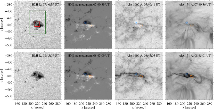
Figure 1: Overview images showing AR 11865 shortly before (top panels) and during (bottom panels) observations. The first two panels of each row show the HMI continuum intensity and line-of-sight magnetic field (values are clipped at $\pm$1500 G), respectively. The last two panels are AIA filtergrams taken in the 1600 Å and 171 Å channels. They are displayed on logarithmic scale and a reversed intensity scaling is used. The times listed in the upper right corner of each panel correspond to the midpoint of the particular HMI or AIA exposure time. The light-blue and orange contours represent the umbrae of opposite polarity within the $\delta$-spot. The green rectangle outlines the full field-of-view of the TIP-II instrument. The red square shows the area displayed in Figs. 6, 7, and 9.

It is often assumed that flares are triggered when shear flows along the PIL build up magnetic shear or twist. Flow fields in a complex and highly active sunspot group were investigated by Deng et al. (2006). They found a shear flow at the PIL of approximately 1 km s^-1 persisting for five hours before an X10 flare occurred. However, after the flare these flows were enhanced and the gradient of the magnetic field changed. Tan et al. (2009) observed a shear flow of 0.6 km s^-1 in a $\delta$-spot between the two umbrae of opposite polarity. After an X3.4 flare, this flow reduced to 0.3 km s^-1. During flaring activity in a $\delta$-spot, Fischer et al. (2012) detected Doppler velocities of $\pm$10 km s^-1. Martinez Pillet et al. (1994) found velocities up to 14 km s^-1. Lites et al. (2002) reported converging flows towards the PIL in the penumbra of a $\delta$-spot. However, Denker et al. (2007) showed that the magnetic shear was not changed significantly by a photospheric shear flow.

Flares are associated with a sudden change in the magnetic field topology. Nevertheless, there are only a few observations which allow us to analyze topological changes of the magnetic field within a $\delta$-spot which are related to a flare. Lately, several studies reported changes in the magnetic field vector during flares. Hudson et al. (2008) predicted that the magnetic field vector changes into horizontal fields during the flare. This is supported by recent findings of Wang et al. (2012) who found a significant increase of the horizontal magnetic field along the PIL related to flare activity. In contrast, Kuckein et al. (2015a, b) reported a strong decrease of the magnetic field strength during the flare, that is, a decrease of both horizontal and vertical components.

Here, we present an analysis of changes of the magnetic field topology of a $\delta$-spot caused by an M-class flare using a unique ground-based data set acquired with the VTT. The data consist of three spectro-polarimetric scans of an area covering a $\delta$-spot during high flaring activity. We focus on variations of the transverse and longitudinal components of the magnetic field. The spectro-polarimetric findings are discussed in the context of high-cadence (E)UV imaging by SDO/AIA.

2 Data and data reduction

Active region (AR) NOAA 11865 was observed on 2013 October 15. The ground-based observations were performed with the Tenerife Infrared Polarimeter (TIP-II; Collados et al. 2007) at the Vacuum Tower Telescope (VTT; von der Lühe 1998) on Tenerife (Spain). As context data, we also used co-temporal (E)UV filtergrams provided by the Atmospheric Imaging Assembly (AIA; Lemen et al. 2012) and line-of-sight magnetograms, Dopplergrams, and continuum intensity images obtained by the Helioseismic and Magnetic Imager (HMI; Scherrer et al. 2012; Schou et al. 2012). Both these instruments are on board the Solar Dynamics Observatory (SDO; Pesnell et al. 2012). The disk-center coordinates of the target were $(x,y)=(220\arcsec,-440\arcsec)$, and the cosine of the heliocentric angle was $\mu=0.86$. The global overview of the observed area shortly before and during the measurements is shown in Figure 1.

2.1 VTT data

The TIP-II instrument was operated in spectropolarimetric mode and measured combinations of the four Stokes parameters along the spectrograph slit. The chosen 1 $\mu$m spectral window comprised two photospheric spectral lines which are formed at slightly different photospheric layers and are sensitive to the magnetic field: Fe i 10783 Å and Si i 10786 Å. For details about these spectral lines we refer to Balthasar & Gömöry (2008), for example.

Three scans (hereafter scans 1, 2, and 3) of 140 steps each with a step size of 0$\aas@@fstack{\prime\prime}$35 were taken between 07:45 and 08:09 UT, 08:10 and 08:33 UT, and 08:37 and 09:00 UT. The exposure time for the infrared camera of TIP-II was 250 ms and the number of accumulations was set to eight. The data calibration included dark-current subtraction, flat-field correction, and the standard polarimetric calibration including a residual cross-talk correction (Collados 1999, 2003; Schlichenmaier & Collados 2002). Data were binned by a factor of two in spectral and spatial directions. Thus, the resulting pixel size along the slit was 0$\aas@@fstack{\prime\prime}$36. The observed spectrum was compared with the near infrared Fourier transform spectrometer atlas (Wallace et al. 1993), and a spectral sampling of 22.17 mÅ per pixel was determined. The inversion procedure requires a normalization of the Stokes profiles to the quiet-Sun intensity at disk center. Thus, we multiplied the data with a limb darkening factor of 0.971 that we obtained from Eq. 2 of Pierce et al. (1977).

Inversions of the full Stokes profiles recorded by the TIP-II instrument were computed with the Stokes Inversions based on Response functions code (SIR; Ruiz Cobo & del Toro Iniesta 1992). The two spectral lines were inverted independently with a one-component model atmosphere. The temperature stratification of this model corresponds to the Harvard Smithsonian Reference Atmosphere (HSRA, Gingerich et al. 1971) and covers the range $-4.4<\log\tau<1.0$. The inversions were performed in three cycles. For the temperature we use one node in the first cycle and three nodes in the second and third cycles. Magnetic field strength, inclination, and azimuth as well as the Doppler velocity were treated as height independent (one node was used for each cycle). We subtracted a fixed amount of 7.5% dispersed stray light from the quiet Sun, and applied a macro turbulence of 1.75 km s^-1.

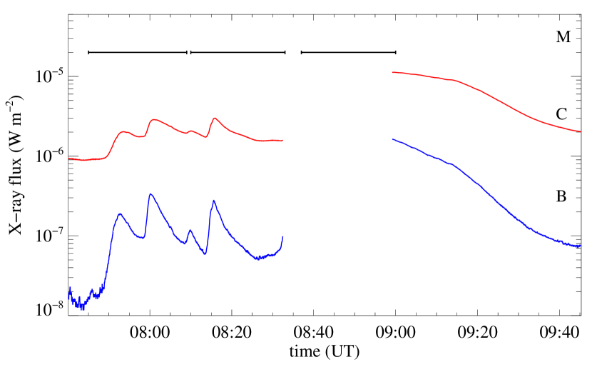
Figure 2: GOES 1–8 Å (red line) and 0.5–4.0 Å (blue line) light curves showing the temporal evolution of the X-ray flux during ground-based observations. We note the gap in the data during the occurrence of the strongest event. The three horizontal black lines correspond to the time of scans 1, 2, and 3 of the VTT.

We tried to solve the magnetic azimuth ambiguity with different methods such as the azimuth center method (see Balthasar 2006), and the method of Leka et al. (2009), but for this complex case we could not find a satisfying solution. Therefore, we consider only the total magnetic field strength and its longitudinal and transverse components in the following.

2.2 SDO data

The SDO/AIA instrument provides multiple, high-resolution full-Sun images (field of view $\sim$1.3 $R_{\odot}$). It carries four telescopes and quasi-simultaneously observes solar transition region and corona at a 12-second cadence in seven different EUV filters, and at a 24-second cadence in two UV filters. The spatial resolution of the acquired filtergrams is $\sim$1$\aas@@fstack{\prime\prime}$5 with a corresponding pixel size of 0$\aas@@fstack{\prime\prime}$6 $\times$ 0$\aas@@fstack{\prime\prime}$6.

The SDO/HMI instrument takes full-disk observations of the Sun at six wavelength positions distributed at $\pm$34.4 mÅ, $\pm$103.2 mÅ, and $\pm$172 Å around the center of the photospheric Fe i 6173.34 Å absorption line. The acquired filtergrams are combined to form simultaneous continuum intensity images, line-of-sight magnetograms and Dopplergrams at a 45-second temporal cadence and with an image scale of 0$\aas@@fstack{\prime\prime}$5 per pixel. The longitudinal magnetograms are obtained with a noise level of 10 G.

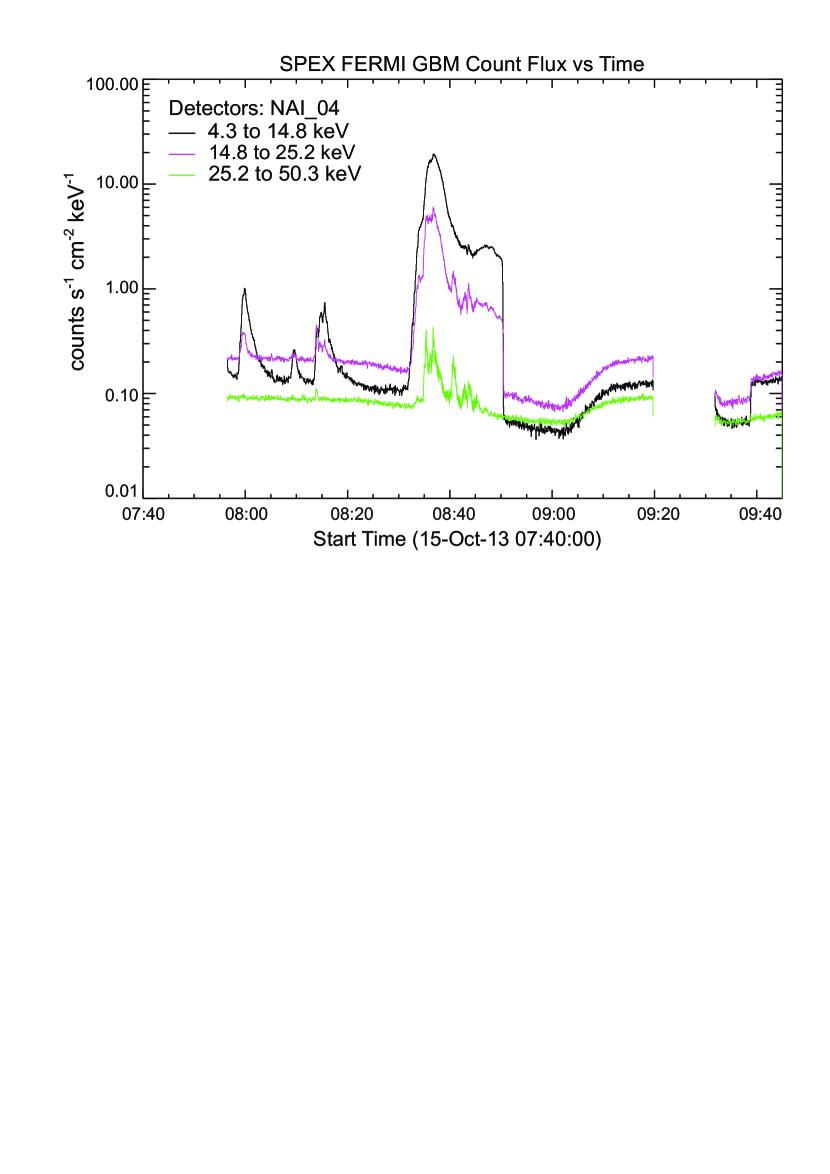
Figure 3: FERMI (4–50 keV, color-coded lines) X-ray light curves covering the same time range as shown in Fig. 2. The displayed data provide complementary information as they fill the gap in the GOES measurements.

AIA and HMI data were downloaded from the Virtual Solar Observatory (VSO) in level 1.0 and 1.5 format, respectively. In this format the data from both instruments have already been partially processed. For AIA data, the pre-processing includes: bad-pixel removal, despiking and flat-fielding. But the data were not exposure-time corrected. In case of HMI data, they were also photometrically corrected. Moreover, images of the physical observables (i.e., continuum images, magnetograms, and Dopplergrams) were already created from individual filtergrams. All data were then processed using aia$\_$prep.pro which is part of the SolarSoft software library implemented within the Interactive Data Language (IDL). This adjusts all of the different AIA filter images as well as HMI data products to a common plate scale so that they share the same centers, rotation angles, and image scales. At the end, all data were spatially derotated to the same reference frame in order to compensate the differential solar rotation.

As the plasma parameters can evolve quickly in active regions, the observation times have to be stated very precisely when comparing data from different instruments. Therefore, we always use the midpoint of the particular exposure (given in UT) if we refer to individual exposures of AIA and HMI data products.

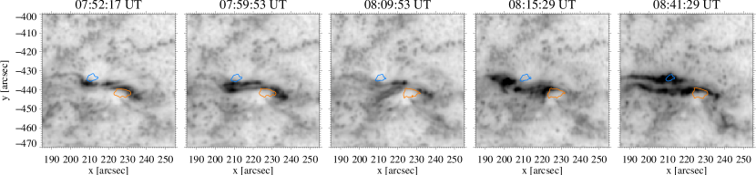
Figure 4: Sequence of AIA 1600 Å filtergrams showing almost continuous flaring activity within the $\delta$-spot of the AR 11865 during observations. The logarithmic scale and a reversed intensity scaling is used to display the data. The midpoint of the recording time of the particular images is presented above each panel. The light-blue and orange contours represent the umbrae of negative and positive polarity within the spot, respectively. The full time resolution animation of the displayed wavelength channel is shown in the online movie.

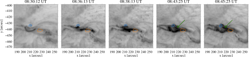
Figure 5: AIA 171 Å filtergrams at five different times showing temporal changes of coronal structures during the observed M-class flare. In particular, the images show the temporal evolution of flare loops (marked by the green arrows) which connect the umbrae within the $\delta$-spot. This feature was not visible before, during the impulsive phase and the peak time of the flare (first three panels) but appeared shortly after the flare’s X-ray flux reached its maximum (last two panels). The logarithmic scale and a reversed intensity scaling is used again. The times above each panel correspond to the midpoint of the particular recording time. The contours have the same meaning as in Fig. 4. The full time resolution animation at this wavelength is also available as a part of the online movie.

3 Results

3.1 Activity in AR 11865

The NOAA AR 11865 was initially detected on the visible part of the solar disk on 2013 October 9 and was classified as $\beta$-type according to the Hale classification. However, already on the next day, the $\delta$-configuration of the leading spot developed. Since that time, the AR 11865 activated and produced C-class flares every day and also, exceptionally, M-class events. On the day of our observations (2013 October 15), the active region became highly active and produced eight C- and one M-class flares.

The recorded GOES data (see Fig. 2) shows that four C-class flares of slightly different magnitude as well as one M-class flare appeared during our ground-based observations. There is a gap in the GOES data exactly at the moment when the strongest flare appeared because the satellite entered the Earth’s shadow. Thus, we cannot identify its real amplitude. The existing data cover only the declining phase of that flare and indicate that the flare level was at least M1.8. Therefore, we refer to it as an M-class event in the following text.

Fortunately, the FERMI satellite (Atwood et al. 2009), captured the temporal evolution of the X-ray emission during this event. Figure 3 shows the light curves in three FERMI energy bands for the same time range as displayed in Fig. 2. The time between 07:55 UT and 08:50 UT is well covered by FERMI measurements, thus showing four out of five events detected by GOES (only the first event is missed). More importantly, the impulsive as well as peak phase of the main M-class event (but not its decay) is detected. Thus, the combination of the FERMI and GOES measurements allow us to also determine precise timing for the strongest event. It started at 08:31 UT, peaked at 08:38 UT (there is also secondary peak visible at 08:48 UT) and lasted longer than the ground-based observations. At 08:50 UT, FERMI also entered Earth’s shadow, and the signals dropped suddenly. Our ground-based observations did not cover the main impulsive phase of the flare very well.

The very high activity related to the studied $\delta$-spot during its observations is demonstrated also in Fig. 4 (see attached movie). It shows a series of the AIA 1600 Å images taken at the moments when the flares indicated by GOES and FERMI X-ray light curves occurred (cf. Figs. 2 and 3). The activity is mostly visible along the PIL which separates opposite magnetic polarities within the $\delta$-spot but some of the stronger C-class eruptions also show a typical two-ribbon structure with the ribbons parallel to the PIL.

The origin of the largest event is also located in the $\delta$-spot of AR 11865 but in this case it extensively expands to its surroundings reaching also AR 11864. The AIA 1600 Å filtergrams show two clearly discernible bright ribbons starting on 08:39 UT, which separate in opposite directions. Their roots are at the PIL of the $\delta$-spot. The two ribbons are seen in all AIA wavelength bands.

Flaring activity related to the $\delta$-spot was also visible in the corona. For example, the AIA 171 Å channel, which probes coronal temperatures, exhibited lots of flare-related dynamics. The activity occurred mainly along the PIL (i.e., co-spatially with the flare brightenings observed in the 1600 Å channel) and only very sporadic and short-lived magnetic loops bridging the neutral magnetic line were detected during four C-class events (for details see online movie). Then, a significant new system of hot loops, which connected the umbrae within the $\delta$-spot, appeared during the strongest flare.

The evolution of this coronal structure is shown in Fig. 5. The first three panels of Fig. 5 represent moments slightly before and during the impulsive phase, and during the peak time of the M-class flare. Here the flare related dynamics started to be obvious again with increasing time but the brightenings were still localized mainly along the PIL. Then, at 08:41 UT, a new system of loops centered at around $(x,y)\approx$ ($219$″, $-438$″), which connects the umbrae of opposite polarities, became visible for the first time (see online movie). This coronal structure became more clear at 08:43 UT and was best visible at 08:45 UT (see last two panels of Fig. 5). The indications of the observed loops remained detectable at least until 08:51 UT. Thus, their appearance is co-temporal with scan 3 from the VTT. However, we cannot exclude that the loop system was present in the upper atmosphere much earlier than discussed above and became temporarily visible later when it was filled with plasma heated by the M-class flare. We note that this structure was not visible in the AIA 1600 Å and 1700 Å images, which map a lower height in the atmosphere.

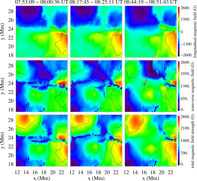
Figure 6: From top to bottom: longitudinal, transverse, and total magnetic field strength inferred from the Fe i 10783 Å inversions. Cutouts from scans 1, 2, and 3 showing internal area of the $\delta$-spot related to the observed changes of the magnetic field are displayed from left to right. The axes in $Mm$ are used in order to allow easier verification of determined parameters listed in the text (e.g., values entering Equation 1). The red arrow marks an enhanced patch of transverse magnetic field detected in scan 3 (i.e., during the M-class flare). The black lines represent umbrae of the $\delta$-spot.

The strongest flare was also associated with the eruption of a filament and coronal loop system as observed in AIA, and a slow and faint CME (v $\approx$ 220 km s^-1) observed by SOHO/LASCO (for more details see LASCO CME catalog: https://cdaw.gsfc.nasa.gov/).

3.2 Magnetic field

The SIR results provide the magnetic field strength inferred from the Stokes parameters. The longitudinal and transverse components of the magnetic field are computed by multiplying the magnetic field strength by $\cos\theta$ and $\sin\theta$, respectively, where $\theta$ is the line-of-sight (LOS) inclination of the magnetic field lines. We were limited to this approach as we were not able to solve the azimuth ambiguity because of the complicated magnetic structure of the observed $\delta$-spot.

The Si i spectral line forms roughly 100–150 km higher compared to Fe i. Both lines sample very low atmospheric heights (Balthasar & Gömöry 2008). Therefore, the overall inferred magnetic field strength is similar at both heights, but as expected, it is slightly weaker in the Si i line (see Figs. 6 and 7).

In all three scans, the longitudinal component of the magnetic field does not show any significant changes. In general, only small and spatially very localized variations (i.e., small increases as well as decreases) were detected. Thus, probably the only noteworthy change is the appearance of the negative longitudinal field inside the northern part of PIL. This is seen as a slight downward deformation of the negative polarity patch visible at coordinates around $(x,y)\approx$ ($15-20$ Mm, $23-24$ Mm) in the top-rightmost panels (corresponding to scan 3) of Figs. 6 and 7.

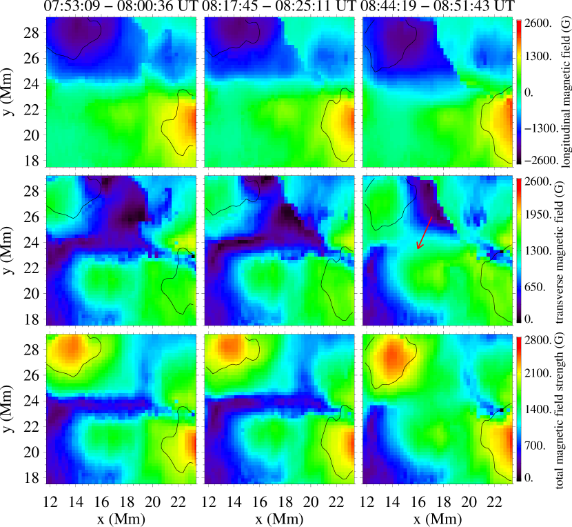
Figure 7: As in Fig. 6 but for the inversions of Si i 10786 Å spectral line.

However, a significant patch of the transverse component appeared at the PIL at around $(x,y)\approx$ ($14-20$ Mm, $20-25$ Mm) (see the red arrow in Figs. 6 and 7) in the last scan (after the flare). This patch bridges the PIL and connects the umbrae within the $\delta$-spot. Fig. 8 shows the observed and calculated Stokes profiles for one pixel next to the PIL where we encounter the increase of the horizontal magnetic field during the flare. In general we see a reasonable agreement of observed and inverted profiles. Therefore, a one-component inversion applied to data is justified. Only for the few cases of anomalous but weak Stokes-$V$ profiles could a two component inversion yield better fits. Nevertheless, there is an obvious increase of the Stokes-$U$ amplitude after the flare.

An increase of approximately 550 G with respect to scans 1 and 2 is visible in Figs. 6 and 7 in the area marked by the red arrow. The bottom panels show the total magnetic field, which in turn also shows an increase in the above mentioned area.

The newly occurred patch of increased transverse magnetic field is co-spatial and co-temporal with the newly formed system of hot flare loops visible in the AIA 171 Å images, which also connects umbrae within the observed spot (cf. Fig. 5). Thus, the natural question is whether these two magnetic structures visible at very different temperatures (and also heights) are related to each other or not.

An inspection of the HMI magnetograms between 07:45 and 09:00 UT (co-temporal to the VTT observations) shows that both polarities were close together in the $\delta$-spot, only separated by a thin PIL. As the M-class flare approached in time, the positive polarity next to the PIL gradually vanished, that is, LOS magnetic flux slowly disappeared. This visually produces a widening of the PIL. Most of the positive polarity close to the border of the PIL disappeared once the flare happened.

3.3 Doppler velocities

The LOS velocities derived from the Fe i and Si i inversions are shown in Fig. 9. The same small cutout of the $\delta$-spot as in Figs. 6 and 7 is shown. The panels representing scan 1 show an extended redshifted area bridging both umbrae. Moreover, there is a patch of strong redshifts (visible mainly in Fe i) close to the umbra of positive polarity. However, this patch disappears already in the second scan and only blueshifts are seen along almost the whole PIL. These significant changes are probably caused by the high flaring activity during the observations. On the other hand, blueshifts at the PIL are clearly visible also in the panels corresponding to scan 3. Thus, this structure was not significantly affected by the M-class flare and surprisingly also not by a newly formed patch of the transverse magnetic component. This is also supported by HMI Dopplergrams (not shown here), which show predominantly blueshifted PIL during the whole M-class flare.

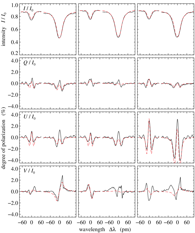
Figure 8: Observed Stokes profiles for a selected location near the PIL displayed as solid black lines, and the results from the SIR-inversion overlaid as red dashed lines. In the left part of each panel, Fe i 10783 Å is shown, and in the right part, Si i 10786 Å. The columns stand for the three scans, and from top to bottom, Stokes $I/I_{0}$, $Q/I_{0}$, $U/I_{0}$ and $V/I_{0}$ are shown.

4 Discussion

The $\delta$-spot was embedded in an active region that produced many flares over its lifetime (see Figs. 2, 3, and 4). All AIA wavelength bands showed eruptive events during our ground-based observations. The HMI magnetograms showed a widening of the PIL, especially after the eruption of an M-class flare, revealing that the magnetic field topology was undergoing changes. Supporting evidence for this can be found in the inferred magnetic field vector from the two low-lying photospheric Fe i 10783 Å and Si i 10786 Å spectral lines. After the flare, a patch of transverse magnetic field developed at the PIL (see Figs. 6 and 7), which increased the total magnetic field in the corresponding region as well.

This result fits well into recent predictions (e.g., Hudson et al. 2008) and observations (e.g., Wang et al. 2012) where the photospheric magnetic field tilts toward a more horizontal configuration after a flare, that is, parallel to the surface. Flare-associated changes of the magnetic field in observations and simulations were also studied by Li et al. (2011) who similarly reported an enhancement in the horizontal magnetic field near the flaring PIL. They explain these changes as a natural consequence of the lift-off of the pre-existing coronal flux rope, and the subsequent implosion of the magnetic field with inward collapsing post-reconnection loops above the PIL. The topical M-class flare was followed by the appearance of a new system of coronal loops connecting umbrae within the $\delta$-spot as seen in the lower rightmost panel of Fig. 1 and in Fig. 5. They may correspond to the lifted-off flux rope described in Li et al. (2011). A comprehensive study of flare-induced changes in the photospheric and chromospheric magnetic field is presented in Kleint (2017). The author found that the changes of the photospheric magnetic field due to an X1 flare are located near the PIL.

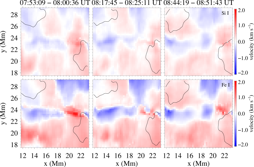
Figure 9: LOS velocities inferred using SIR inversions of Fe i (bottom panels) and Si i (top panels) spectral lines. The velocities are clipped between $\pm 2$ km s^-1. The black contours represent the umbrae of the $\delta$-spot.

A detailed inspection of our results suggests that the changes of the photospheric magnetic field closely coincide with the PIL and seem to follow its shape (Figs. 1, 6, and 7). These results also suggests that the field topology suffered the changes mostly in an elongated PIL-aligned area centered at $(x,y)\approx(15,24)$ Mm with an approximate size of $5$ Mm (region marked by the red arrow in Figs. 6 and 7), where the area-averaged changes of both the transverse field $\left<\delta B_{TR}\right>$ and total magnetic field increased, on average, by approximately 550 G. The changes of the longitudinal magnetic field $\left<\delta B_{LOS}\right>$ do not reach more than 200 G in the area close to or within the PIL.

Fisher et al. (2012) used the concept of momentum conservation and assessed the Lorentz-force changes due to the release of energy associated with the rapid evolution of the coronal magnetic field. They argue that a back-reaction following flares could push the photospheric magnetic fields to become more horizontal near the flaring PIL. These authors estimated the changes of the radial Lorentz force $\delta F_{r}$ (LF) exerted on the photosphere from the corona to be

$$\delta F_{r}=\frac{1}{8\pi}\int_{A_{ph}}\left(\delta B_{LOS}^{2}-\delta B_{TR}^{2}\right)dA\approx\frac{1}{8\pi}\left\{\left<\delta B_{LOS}\right>^{2}-\left<\delta B_{TR}\right>^{2}\right\}A_{ph}.$$ (1)

The surface integral involves the photospheric domain experiencing the magnetic field changes. From its estimated area $A_{ph}\approx 5$ Mm² and the values given before follows $\delta F_{r}\approx 5.3\times 10^{20}$ dyn. This value is almost one order of magnitude smaller than the downward LF change of $3.2\times 10^{21}$ dyn estimated in Su et al. (2013) for the B4.2-class flare in AR NOAA 8027 on 1997 April 9, which was caused by a tiny negative feature invading its surrounding positive polarity region. Our estimate is also almost two orders of magnitude smaller than the LF change of $1.6\times 10^{22}$ dyn reported in Wang & Liu (2010) for the 2002 July 26 M8.7 flare. They found similar values of the LF change for several other X-class flares. For comparison, Xu et al. (2016) estimated the LF peak value at approximately $1\times 10^{22}$ dyn, which was associated with the X1.1 flare in the $\delta$-configuration region in the following part of AR 11890.

Unfortunately, in our case, the slit did not catch the highest emission of the flare. Therefore, we cannot estimate the changes in the magnetic field during the peak of the flare. Such a study is reported by Kuckein et al. (2015a, b) who showed a huge drop in the photospheric magnetic field during the maximum of the flare.

Remarkably, the LOS velocity maps in Fig. 9 do not show any significant changes of velocity patterns, which might be associated with the observed M-class flare. The area coinciding with the magnetic field changes at $(x,y)\approx$ (15, 24) Mm at the PIL is characterized by a persistent upflow of approximately $-1$ kms^-1. This behavior is confirmed by HMI Dopplergrams, which sample the region with much better temporal resolution.

The quasi-invariability of the upflow could be due to very different optical depths, where the velocity response function and the magnetic field response function have their maxima. Another possibility to explain the ground-based observations would be that the slow scanning simply missed the moment of occurrence of short-living/temporary velocity changes induced by the flare. However, this scenario is excluded by SDO/HMI measurements. On the other hand, we cannot exclude that the spatial resolution of our observation was insufficient to resolve the probably very subtle flare-induced velocity changes. Kuckein et al. (2015a) reported on newly appearing upflows in response to an M3.2 flare. Although their data were taken with the same instrument, the upflows were stronger next to the PIL rather than along it. However, their flare was not related to a $\delta$-spot and might consequently show different properties. Steady, persistent, and subsonic motions were observed along the PIL of a $\delta$-spot also by Cristaldi et al. (2014). They reported a stable pattern of upflows and downflows of $\pm$3 km s^-1 along the PIL detected by ground-based high-resolution observations. The presence of this pattern was confirmed by HMI measurements. Based on satellite data, they estimated that the flows lasted for at least 15 hours.

Finally, we recall that the increase of the transverse photospheric field is cospatial and cotemporal with the new, hot flare loops visible in the AIA 171 Å channel (the lower rightmost panel of Fig. 1 and Fig. 5). Likely, these are only two facets of magnetic field changes cascading across the flaring atmosphere, yet we cannot confirm this hypothesis using our data.

5 Conclusions

We present rare ground-based spectro-polarimetric observations of the flaring $\delta$-spot performed by the TIP-II instrument attached to the spectrograph of the VTT. We found very stable magnetic configuration which remains almost unchanged during a sequence of four C-class flares. However, after the strongest flaring event, we discovered a significant increase of approximately 550 G in the transverse magnetic field in places connecting umbrae of opposite polarities. The observations taken by the SDO/AIA instrument in the 171 Å channel revealed the formation of the new system of magnetic loops which also connects umbrae within the observed $\delta$-spot. This suggests that formation of a new system of loops reaching from photosphere up to corona was induced/triggered by the M-class flare. The Doppler velocities estimated from the spectro-polarimetric scans as well as from measurements provided by the SDO/HMI instrument do not show any significant changes in the plasma flows during formation of the aformentioned magnetic loops.