A Geometric Approach to Covariance Matrix Estimation and its Applications to Radar Problems

A. Aubry, Senior Member, IEEE, A. De Maio Fellow, IEEE, and L. Pallotta, Member, IEEE A. Aubry and A. De Maio (corresponding author) are with Università degli Studi di Napoli “Federico II”, Dipartimento di Ingegneria Elettrica e delle Tecnologie dell’Informazione, Via Claudio 21, I-80125 Napoli, Italy. E-mail: augusto.aubry@unina.it, ademaio@unina.it.L. Pallotta is with CNIT, viale G.P. Usberti, n. 181/A - 43124 Parma, c/o udr Università “Federico II”, via Claudio 21, I-80125 Napoli, Italy. E-mail: luca.pallotta@unina.it.
Abstract

A new class of disturbance covariance matrix estimators for radar signal processing applications is introduced following a geometric paradigm. Each estimator is associated with a given unitary invariant norm and performs the sample covariance matrix projection into a specific set of structured covariance matrices. Regardless of the considered norm, an efficient solution technique to handle the resulting constrained optimization problem is developed. Specifically, it is shown that the new family of distribution-free estimators shares a shrinkage-type form; besides, the eigenvalues estimate just requires the solution of a one-dimensional convex problem whose objective function depends on the considered unitary norm. For the two most common norm instances, i.e., Frobenius and spectral, very efficient algorithms are developed to solve the aforementioned one-dimensional optimization leading to almost closed form covariance estimates. At the analysis stage, the performance of the new estimators is assessed in terms of achievable Signal to Interference plus Noise Ratio (SINR) both for a spatial and a Doppler processing assuming different data statistical characterizations. The results show that interesting SINR improvements with respect to some counterparts available in the open literature can be achieved especially in training starved regimes.

Index Terms:
Adaptive Radar Signal Processing, Structured Covariance Matrix Estimation, Unitary Invariant Matrix Norm, Projection, Condition Number.

I Introduction

Interference covariance matrix estimation is a longstanding and basic problem in adaptive radar signal processing and naturally arises in several areas such as target detection, direction of arrival estimation, sidelobe cancelling, and secondary data selection [1, 2, 3, 4] (just to list a few). Conventional adaptive architectures (such as Sample Matrix Inversion (SMI) Doppler filter [1], Kelly’s receiver [4], and spatial beamformers [5]) resort to the sample covariance matrix of a secondary data set collected from range gates spatially close to the one under test to estimate the interference covariance. These algorithms are often very prohibitive because they lean on the assumption that the environment remains stationary and homogeneous during the adaptation process. Precisely, they provide satisfactory performance when the secondary vectors share the same spectral properties of the interference in the test cell, are statistical independent, and their number is higher than twice the useful signal dimension [1]. These requisites however may represent important limitations since in real environments the number of data where the disturbance is homogeneous (often referred to as sample support) is very limited. Besides, poor training data selection, in such adaptive algorithms, can result in severe radar performance degradation [6] and [7].
A viable means to thwart the lack of a sufficient number of homogeneous secondary data is to capitalize some a-priori information about the radar surrounding environment, namely to realize a knowledge-based/cognitive processing [8] so as to restrict the uncertainty region of the unknown parameters. According to this processing paradigm, several approaches have been pursued in the open literature assuming different structural models as well as statistical distributions of the data. In particular, both homogeneous and heterogeneous interference environments are dealt with. As to the former scenario, the training data are modeled as independent and identically distributed (i.i.d.), zero-mean, circularly symmetric Gaussian vectors. Whereas, the latter context mainly considers clutter power variations within the sample support. Thus, assuming homogeneity, in [9] the Maximum Likelihood (ML) covariance matrix estimator is derived modeling the disturbance as the sum of a coloured interference plus white disturbance; in [10], the ML estimation of an unstructured covariance matrix with a condition number upper bound requirement is considered; in [11], using the same covariance structure as in [9], the ML estimator is derived when a constraint on the condition number is imposed too; in [12], a rank-constrained ML estimator is developed; furthermore, relying on a Mean Square Error (MSE) design criterion, in [13] and [14], some shrinkage estimators are proposed. With reference to heterogeneous scenarios, compound Gaussian statistical models (such as K-distributed or Gamma amplitudes) are usually exploited to account for clutter returns spikiness. In [15], assuming a clutter dominated environment, a unified framework to regularize the ML estimate in scaled Gaussian models (e.g., elliptical distributions, compound-Gaussian processes and spherically invariant random vectors) is developed in order to enhance Tyler’s estimator in the presence of a small sample support exploiting a-priori information on the covariance structure. In [16], Tyler’s robust covariance M-estimator under group symmetry constraints, such as circulant, persymmetric, and proper quaternion matrices, is considered. Precisely, it is provided an iterative fixed point algorithm to compute the constrained estimate. Finally, in [17], an iterative algorithm to estimate, according to the ML approach, both the clutter subspace and the covariance is proposed, assuming the disturbance composed of a low rank compound Gaussian clutter plus a white Gaussian noise contribution. Further technically sound and effective covariance estimators can be found in [18, 19, 20, 21, 22, 23].
These mentioned algorithms lean on specific assumptions about the data statistical characterization and may suffer performance loss in the presence of model mismatches due to for instance quantization effects, constant modulus jamming signals, phase noise [24, 25, 26]. To overcome this shortcoming and endow robustness to the estimation process, some strategies derived from geometric considerations on the metric space of the covariance matrices have been also developed. In this respect, in [27] and [28] techniques based on Riemannian p𝑝p-mean (e.g., Fréchet median and Karcher barycenter) evaluation are developed to estimate suitably structured interference covariance matrices showing that substantial ameliorations over classical algorithms can be attained. In [27] and [29] also an extension of the conventional Ordered Statistic (OS) framework [30] is proposed relying on the Riemannian p𝑝p-mean computation of Toepliz or Toeplitz-Block-Toeplitz space-time covariance matrices. Besides, in [31] and [32], covariance estimates defined through geometric barycenters/medians (associated with specific distances in the space of Hermitian matrices) of structured covariance estimates are exploited both for training data selection and adaptive radar detection highlighting significant gains with respect to the classic sample covariance matrix. Finally, in [33, 34, 35, 36, 37, 38] other interesting geometric-inspired procedures are devised.
In this paper, leveraging on a geometric criterion, a novel class of covariance estimators that do not consider any assumption on the statistical characterization of the secondary data is proposed and analyzed. Each estimator is associated with a given unitary invariant norm and performs the sample covariance matrix projection into a specific set of structured covariance matrices. Precisely, this set encompasses the matrices modeled as the sum of an unknown positive semi-definite matrix (describing coloured interference and clutter) plus a term proportional to the identity matrix (related to white disturbance). Besides, a constraint on the condition number is accounted for so as to control the numerical stability of the resulting adaptive algorithms [5]. Regardless of the considered norm, an efficient solution technique to handle the formulated constrained optimization problem is developed. Precisely, each estimator exhibits a shrinkage-type form and its evaluation requires the sample covariance matrix spectral decomposition as well as the solution of a one-dimensional convex problem whose objective function depends on the considered unitary norm.
At the analysis stage, the performance of the new class of distribution-free estimators is evaluated in terms of achievable Signal-to-Interference-plus-Noise Ratio (SINR) for different sample support sizes, assuming both a spatial and a Doppler processing scenario. The results show that interesting SINR improvements can be achieved with respect to some counterparts available in the open literature also with a reduced computational complexity.
The remainder of this paper is organized as follows. Section II is devoted to the description of the system model as well as the formulation of the covariance matrix estimation problem. In Section III, an efficient procedure to solve the resulting constrained optimization is developed. In Section IV, the performance of the proposed distribution-free estimators is assessed. Finally, Section V concludes the paper and provides some possible future research tracks.

Notation

We adopt the notation of using boldface for vectors 𝒂𝒂a (lower case), and matrices 𝑨𝑨A (upper case). The transpose and the conjugate transpose operators are denoted by the symbols ()Tsuperscript𝑇(\cdot)^{T} and ()superscript(\cdot)^{\dagger} respectively. tr{}tr\mbox{\rm tr}\,\{\cdot\} is the trace of the square matrix argument. 𝑰𝑰I and 𝟎0{\bf 0} denote respectively the identity matrix and the matrix with zero entries (their size is determined from the context). diag(𝒂)diag𝒂\mbox{\boldmath\bf diag}\,(\mbox{\boldmath{$a$}}) indicates the diagonal matrix whose i𝑖i-th diagonal element is the i𝑖i-th entry of 𝒂𝒂a. Nsuperscript𝑁{\mathbb{R}}^{N}, Nsuperscript𝑁{\mathbb{C}}^{N}, N,Ksuperscript𝑁𝐾{\mathbb{C}}^{N,K}, and Nsuperscript𝑁{\mathbb{H}}^{N} are respectively the sets of N𝑁N-dimensional vectors of real numbers, of N𝑁N-dimensional vectors of complex numbers, of N×K𝑁𝐾N\times K matrices of complex numbers, and of N×N𝑁𝑁N\times N Hermitian matrices. The curled inequality symbol succeeds-or-equals\succeq (and its strict form succeeds\succ) is used to denote generalized matrix inequality: for any 𝑨N𝑨superscript𝑁\mbox{\boldmath{$A$}}\in{\mathbb{H}}^{N}, 𝑨𝟎succeeds-or-equals𝑨0\mbox{\boldmath{$A$}}\succeq\mbox{\boldmath{$0$}} means that 𝑨𝑨A is a positive semi-definite matrix (𝑨𝟎succeeds𝑨0\mbox{\boldmath{$A$}}\succ\mbox{\boldmath{$0$}} for positive definiteness). \|\cdot\| denotes an arbitrary unitary invariant matrix norm operator, while the specific spectral and Frobenius instances are indicated by 2\|\cdot\|_{2} and F\|\cdot\|_{F}, respectively. The letter j𝑗j represents the imaginary unit (i.e. j=1𝑗1j=\sqrt{-1}). For any complex number x𝑥x, |x|𝑥|x| represents the modulus of x𝑥x. Finally, 𝔼[]𝔼delimited-[]{\mathbb{E}}\left[\cdot\right] denotes statistical expectation and for any optimization problem 𝒫𝒫{\cal{P}} v(𝒫)𝑣𝒫v({\cal{P}}) represents its optimal value.

II Problem Formulation

In this section, the problem of estimating the covariance matrix 𝑴N𝑴superscript𝑁\mbox{\boldmath{$M$}}\in\mathbb{H}^{N} of K𝐾K secondary data 𝒓1,,𝒓Ksubscript𝒓1subscript𝒓𝐾\mbox{\boldmath{$r$}}_{1},\ldots,\mbox{\boldmath{$r$}}_{K} modeled as N𝑁N-dimensional, circularly symmetric, zero-mean random vectors, is addressed. It is assumed that these vectors share the same second order statistical characterization, i.e.,

𝔼[𝒓i𝒓i]=𝑴,for i=1,,K,formulae-sequence𝔼delimited-[]subscript𝒓𝑖superscriptsubscript𝒓𝑖𝑴for 𝑖1𝐾{\mathbb{E}}[\mbox{\boldmath{$r$}}_{i}\mbox{\boldmath{$r$}}_{i}^{\dagger}]=\mbox{\boldmath{$M$}},\quad\text{for }i=1,\ldots,K, (1)

but are drawn from an arbitrary and unknown joint probability distribution.

According to the previous assumptions, classic estimation approaches such as the ML or the minimum MSE strategies can be no longer pursued since they need the data statistical distribution knowledge. Hence, in this work a new family of covariance estimators based on geometric considerations is introduced. Specifically, the idea is to estimate the data covariance matrix performing the projection111Notice that, the projection operator is usually defined assuming the reference set being convex and closed as well as the norm being induced by an inner product. Nevertheless, with a slight abuse of notation, in this paper we continue to define as projection the point 𝒙psubscript𝒙𝑝\mbox{\boldmath{$x$}}_{p} minimizing the distance (based on a specific metric) between a given point 𝒙𝒙x and the reference set as long as the point 𝒙psubscript𝒙𝑝\mbox{\boldmath{$x$}}_{p} can be uniquely identified., as induced by a specific metric, of the sample covariance matrix

𝑺^=1Ki=1K𝒓i𝒓i,^𝑺1𝐾superscriptsubscript𝑖1𝐾subscript𝒓𝑖superscriptsubscript𝒓𝑖\widehat{\mbox{\boldmath{$S$}}}=\frac{1}{K}\sum_{i=1}^{K}\mbox{\boldmath{$r$}}_{i}\mbox{\boldmath{$r$}}_{i}^{\dagger}, (2)

into the set

{𝑴=𝑹+σn2𝑰,𝑹𝟎,σn2σ2,λmax(𝑴)λmin(𝑴)κM,casesmissing-subexpression𝑴𝑹superscriptsubscript𝜎𝑛2𝑰missing-subexpressionsucceeds-or-equals𝑹0missing-subexpressionsuperscriptsubscript𝜎𝑛2superscript𝜎2missing-subexpressionsubscript𝜆𝑚𝑎𝑥𝑴subscript𝜆𝑚𝑖𝑛𝑴subscript𝜅𝑀\left\{\begin{array}[c]{ll}&\mbox{\boldmath{$M$}}=\mbox{\boldmath{$R$}}+\sigma_{n}^{2}\mbox{\boldmath{$I$}},\\ &\mbox{\boldmath{$R$}}\succeq{\bf 0},\\ &\sigma_{n}^{2}\geq\sigma^{2},\\ &\frac{\lambda_{max}\left(\mbox{\boldmath{$M$}}\right)}{\lambda_{min}\left(\mbox{\boldmath{$M$}}\right)}\leq\kappa_{M},\end{array}\right. (3)

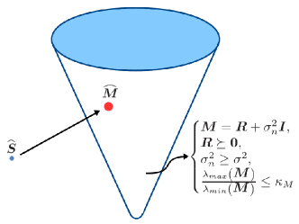
where σ2>0superscript𝜎20\sigma^{2}>0 is a lower bound to the white interference power, 𝑹𝑹R accounts for the colored interfering contribution, and κM1subscript𝜅𝑀1\kappa_{M}\geq 1 is an upper bound to the covariance condition number. This uncertainty set accounts for an interference covariance structure that is commonly met in adaptive radar signal processing applications and ensures a well conditioned estimate necessary to compute the adaptive radar weight vector. The effectiveness of this model has already been proved in [11], where the training data are assumed i.i.d., zero-mean, circularly symmetric Gaussian vectors and the ML estimate is derived. Hence, the main goal of this work is the development of a distribution-free approach which provides a robust alternative to [11] when inference on the interference statistics is not possible. A pictorial representation of the geometric-based estimation process is reported in Fig. 1.
Refer to caption
Figure 1: Projection of the sample covariance matrix into a specific set through a unitary invariant matrix norm.

Following the above guidelines, the covariance matrix estimate 𝑴^^𝑴\widehat{\mbox{\boldmath{$M$}}} is obtained as solution to the following optimization problem

𝒫{min𝑴𝑴𝑺^||s.t.λmax(𝑴)λmin(𝑴)κMσn2𝑰+𝑹=𝑴𝑹𝟎σn2σ2,{\cal{P}}\left\{\begin{array}[c]{ll}\underset{\mbox{\boldmath{$M$}}}{\min}&\begin{array}[c]{c}\|\mbox{\boldmath{$M$}}-\widehat{\mbox{\boldmath{$S$}}}||\end{array}\\ \mbox{s.t.}&\begin{array}[t]{l}\frac{\lambda_{max}\left(\mbox{\boldmath{$M$}}\right)}{\lambda_{min}\left(\mbox{\boldmath{$M$}}\right)}\leq\kappa_{M}\\ \sigma_{n}^{2}\mbox{\boldmath{$I$}}+\mbox{\boldmath{$R$}}=\mbox{\boldmath{$M$}}\\ \mbox{\boldmath{$R$}}\succeq{\bf 0}\\ \sigma_{n}^{2}\geq\sigma^{2}\end{array}\end{array}\right., (4)

where \|\cdot\| refers to an arbitrary but given unitary invariant matrix norm [39] that induces a specific metric in the space of the positive semi-definite matrices over which performing the projection. Examples of norms that can be considered in the estimation process are the Frobenius, the spectral, and the Ky Fan norms. In this respect, observe that the first two instances are the most common and widely used norms in the space of Hermitian matrices corroborating the interest toward the family of unitary invariant norms. Remarkably, different estimators can be jointly exploited within a bank/battery of adaptive receivers. More in detail, each detector may resort to a specific norm and the presence of a prospective target is established by means of a suitable fusion logic, such as binary integration or m𝑚m-of-n𝑛n detection [40].

Before concluding this section, it is also worth pointing out that the proposed estimators possess the consistency property as long as the secondary data vectors are statistically independent. Indeed,

𝑴𝑴^norm𝑴^𝑴\displaystyle\|\mbox{\boldmath{$M$}}-\widehat{\mbox{\boldmath{$M$}}}\| \displaystyle\leq 𝑴𝑺^+𝑺^𝑴^norm𝑴^𝑺norm^𝑺^𝑴\displaystyle\|\mbox{\boldmath{$M$}}-\widehat{\mbox{\boldmath{$S$}}}\|+\|\widehat{\mbox{\boldmath{$S$}}}-\widehat{\mbox{\boldmath{$M$}}}\| (5)
\displaystyle\leq 2𝑴𝑺^,2norm𝑴^𝑺\displaystyle 2\|\mbox{\boldmath{$M$}}-\widehat{\mbox{\boldmath{$S$}}}\|, (6)

where the first equation stems from the triangular inequality, while the second inequality follows from the definition of 𝑴^^𝑴\widehat{\mbox{\boldmath{$M$}}}, i.e., it is a minimizer. Now, provided that 𝑴^^𝑴\widehat{\mbox{\boldmath{$M$}}} is a measurable function of the secondary data222A sufficient condition for estimator measurability is reported in the supplementary material., it follows that

𝔼[𝑴𝑴^2]𝔼delimited-[]superscriptnorm𝑴^𝑴2\displaystyle{\mathbb{E}}[\|\mbox{\boldmath{$M$}}-\widehat{\mbox{\boldmath{$M$}}}\|^{2}] \displaystyle\leq 2𝔼[𝑴𝑺^2]2𝔼delimited-[]superscriptnorm𝑴^𝑺2\displaystyle 2{\mathbb{E}}[\|\mbox{\boldmath{$M$}}-\widehat{\mbox{\boldmath{$S$}}}\|^{2}] (7)
\displaystyle\leq 2α2𝔼[𝑴𝑺^F2]0,2𝛼2𝔼delimited-[]superscriptsubscriptnorm𝑴^𝑺𝐹20\displaystyle 2\alpha 2{\mathbb{E}}[\|\mbox{\boldmath{$M$}}-\widehat{\mbox{\boldmath{$S$}}}\|_{F}^{2}]\rightarrow 0, (8)

where the second inequality results from the finite dimension of the space Nsuperscript𝑁\mathcal{H}^{N}, α𝛼\alpha is a specific constant linking the considered norm with the Frobenius one [39, Corollary 5.4.5], and finally the convergence to zero comes from the consistency of the sample covariance estimator. Based on Chebyshev’s inequality [41], the estimation error converges to zero also in probability which is often invoked as the classic definition of consistency.

III Derivation of the Structured Covariance Matrix Estimators Based on Unitary Invariant Norm Projection

This section deals with the development of an efficient procedure to solve Problem 𝒫𝒫{\cal{P}} almost in closed form regardless of the considered norm. Specifically, it is proved that any sample covariance projector belongs to the class of the shrinkage estimators333A shrinkage covariance estimator 𝑴^^𝑴\widehat{\mbox{\boldmath{$M$}}} is a matrix sharing the same eigenvectors as the sample covariance matrix 𝑺𝟎succeeds-or-equals𝑺0\mbox{\boldmath{$S$}}\succeq{\bf 0}, but transforming the eigenvalues, i.e. 𝑴^=𝑼Sdiag([g1(d1,d2,,dN),g2(d1,d2,,dN),,gN(d1,d2,,dN)])𝑼S𝟎^𝑴subscript𝑼𝑆diagsubscript𝑔1subscript𝑑1subscript𝑑2subscript𝑑𝑁subscript𝑔2subscript𝑑1subscript𝑑2subscript𝑑𝑁subscript𝑔𝑁subscript𝑑1subscript𝑑2subscript𝑑𝑁superscriptsubscript𝑼𝑆succeeds-or-equals0\widehat{\mbox{\boldmath{$M$}}}=\mbox{\boldmath{$U$}}_{S}\,\mbox{\boldmath\bf diag}\,([g_{1}(d_{1},d_{2},\ldots,d_{N}),g_{2}(d_{1},d_{2},\ldots,d_{N}),\ldots,\\ g_{N}(d_{1},d_{2},\ldots,d_{N})])\,\mbox{\boldmath{$U$}}_{S}^{\dagger}\succeq{\bf 0}. and the eigenvalues estimate is obtained solving a one-dimensional convex problem whose objective function is tied up to the considered unitary norm. In general, this optimization problem can be solved in polynomial-time using convex solvers such as CVX [42]. In addition, for the two most relevant norm instances, i.e., Frobenius and spectral, very efficient algorithms are provided to tackle the associated one-dimensional optimizations.

As first step toward the solution of 𝒫𝒫{\cal{P}}, let us observe that it is equivalent to the solvable convex problem

𝒫1{min𝑿𝑿𝑺s.t.𝑿𝑰λmax(𝑿)λmin(𝑿)κM,subscript𝒫1cases𝑿norm𝑿𝑺s.t.succeeds-or-equals𝑿𝑰subscript𝜆𝑚𝑎𝑥𝑿subscript𝜆𝑚𝑖𝑛𝑿subscript𝜅𝑀{\cal{P}}_{1}\left\{\begin{array}[c]{ll}\underset{\mbox{\boldmath{$X$}}}{\min}&\begin{array}[c]{c}\|\mbox{\boldmath{$X$}}-\mbox{\boldmath{$S$}}\|\end{array}\\ \mbox{s.t.}&\begin{array}[t]{l}\mbox{\boldmath{$X$}}\succeq\mbox{\boldmath{$I$}}\\ \frac{\lambda_{max}\left(\mbox{\boldmath{$X$}}\right)}{\lambda_{min}\left(\mbox{\boldmath{$X$}}\right)}\leq\kappa_{M}\\ \end{array}\end{array}\right., (9)

where444The interested reader may refer to the supplementary material for the proof. 𝑺=𝑺^/σ2𝑺^𝑺superscript𝜎2\mbox{\boldmath{$S$}}=\widehat{\mbox{\boldmath{$S$}}}/\sigma^{2} and 𝑿=𝑴/σ2𝑿𝑴superscript𝜎2\mbox{\boldmath{$X$}}=\mbox{\boldmath{$M$}}/\sigma^{2}. Next, let us indicate with 𝑺=𝑼S𝚲S𝑼S𝑺subscript𝑼𝑆subscript𝚲𝑆subscriptsuperscript𝑼𝑆{\mbox{\boldmath{$S$}}}={\mbox{\boldmath{$U$}}}_{S}{\mbox{\boldmath{$\Lambda$}}}_{S}{\mbox{\boldmath{$U$}}}^{{\dagger}}_{S} the spectral decomposition of the normalized sample covariance matrix, where 𝚲S=diag([d1,d2,,dN]T)subscript𝚲𝑆diagsuperscriptsubscript𝑑1subscript𝑑2subscript𝑑𝑁𝑇{\mbox{\boldmath{$\Lambda$}}}_{S}=\mbox{\boldmath\bf diag}\,(\left[d_{1},d_{2},\cdots,d_{N}\right]^{T}), with d1d2dNsubscript𝑑1subscript𝑑2subscript𝑑𝑁d_{1}\geq d_{2}\geq\cdots\geq d_{N} the eigenvalues of 𝑺𝑺S arranged in decreasing order, and 𝑼Ssubscript𝑼𝑆{\mbox{\boldmath{$U$}}}_{S} is the unitary matrix whose columns contain the corresponding eigenvectors. Hence, the following lemma holds true.

Lemma III.1

An optimal solution to 𝒫1subscript𝒫1{\cal{P}}_{1} is a shrinkage estimator 𝐗=𝐔S𝚲𝐔Ssuperscript𝐗subscript𝐔𝑆superscript𝚲superscriptsubscript𝐔𝑆\mbox{\boldmath{$X$}}^{\star}={\mbox{\boldmath{$U$}}}_{S}{\mbox{\boldmath{$\Lambda$}}}^{\star}{\mbox{\boldmath{$U$}}}_{S}^{{\dagger}} where 𝚲=diag([λ1,λ2,,λN]T)superscript𝚲diagsuperscriptsuperscriptsubscript𝜆1superscriptsubscript𝜆2superscriptsubscript𝜆𝑁𝑇\mbox{\boldmath{$\Lambda$}}^{\star}=\mbox{\boldmath\bf diag}\,\left(\left[\lambda_{1}^{\star},\lambda_{2}^{\star},\cdots,\lambda_{N}^{\star}\right]^{T}\right) is a solution to the following optimization problem

𝒫2{min𝚲𝚲𝚲Ss.t.𝚲𝑰λmax(𝚲)λmin(𝚲)κM,subscript𝒫2cases𝚲norm𝚲subscript𝚲𝑆s.t.succeeds-or-equals𝚲𝑰missing-subexpressionsubscript𝜆𝑚𝑎𝑥𝚲subscript𝜆𝑚𝑖𝑛𝚲subscript𝜅𝑀{\cal{P}}_{2}\left\{\begin{array}[c]{ll}\underset{\mbox{\boldmath{$\Lambda$}}}{\min}&\|\mbox{\boldmath{$\Lambda$}}-\mbox{\boldmath{$\Lambda$}}_{S}\|\\ \mbox{s.t.}&\mbox{\boldmath{$\Lambda$}}\succeq\mbox{\boldmath{$I$}}\\ &\frac{\lambda_{max}(\mbox{\boldmath{$\Lambda$}})}{\lambda_{min}(\mbox{\boldmath{$\Lambda$}})}\leq{\kappa_{M}}\end{array}\right., (10)

with 𝚲=diag([λ1,λ2,,λN]T)𝚲diagsuperscriptsubscript𝜆1subscript𝜆2subscript𝜆𝑁𝑇\mbox{\boldmath{$\Lambda$}}=\mbox{\boldmath\bf diag}\,\left(\left[\lambda_{1},\lambda_{2},\cdots,\lambda_{N}\right]^{T}\right).

Proof:

See Appendix -A. ∎

To proceed further, let us introduce the auxiliary variable u>0𝑢0u>0 and cast 𝒫2subscript𝒫2{\cal{P}}_{2} as555The interested reader may refer to the supplementary material for the proof.

𝒫2(u){min𝚲,u𝚲𝚲Ss.t.λi1,uλiκMu,u1κM,i=1,,N.formulae-sequencesuperscriptsubscript𝒫2𝑢cases𝚲𝑢norm𝚲subscript𝚲𝑆s.t.subscript𝜆𝑖1missing-subexpression𝑢subscript𝜆𝑖subscript𝜅𝑀𝑢missing-subexpression𝑢1subscript𝜅𝑀𝑖1𝑁{\cal{P}}_{2}^{\prime}(u)\left\{\begin{array}[c]{ll}\underset{\mbox{\boldmath{$\Lambda$}},u}{\min}&\|\mbox{\boldmath{$\Lambda$}}-\mbox{\boldmath{$\Lambda$}}_{S}\|\\ \mbox{s.t.}&\lambda_{i}\geq 1,\\ &u\leq{\lambda_{i}}\leq{\kappa_{M}u},\\ &u\geq{\frac{1}{\kappa_{M}}},\end{array}\right.\quad i=1,\ldots,N. (11)

This formulation paves the way for an efficient solution of 𝒫2subscript𝒫2{\cal{P}}_{2}. Indeed, for any fixed u𝑢u a closed form optimal matrix can be derived as shown in the following lemma.

Lemma III.2

For any u¯1κM¯𝑢1subscript𝜅𝑀\bar{u}\geq\frac{1}{\kappa_{M}}, an optimal solution 𝚲(u¯)superscript𝚲¯𝑢\mbox{\boldmath{$\Lambda$}}^{\star}(\bar{u}) to 𝒫2(u¯)superscriptsubscript𝒫2¯𝑢{\cal{P}}_{2}^{\prime}(\bar{u}), is

𝚲(u¯)=diag(𝝀(u¯)),superscript𝚲¯𝑢diagsuperscript𝝀¯𝑢\mbox{\boldmath{$\Lambda$}}^{\star}(\bar{u})=\mbox{\boldmath\bf diag}\,(\mbox{\boldmath{$\lambda$}}^{\star}(\bar{u})), (12)

where

𝝀(u)=[λ1(u),λ2(u),,λN(u)]TN,superscript𝝀𝑢superscriptsubscript𝜆1𝑢subscript𝜆2𝑢subscript𝜆𝑁𝑢𝑇superscript𝑁\begin{split}\mbox{\boldmath{$\lambda$}}^{\star}(u)=&\left[\lambda_{1}(u),\lambda_{2}(u),\ldots,\lambda_{N}(u)\right]^{T}\in\mathbb{R}^{N},\end{split} (13)

with

λi(u)=min(κMu,max(di,max(1,u))),i=1,,N.formulae-sequencesubscript𝜆𝑖𝑢subscript𝜅𝑀𝑢subscript𝑑𝑖1𝑢𝑖1𝑁\lambda_{i}(u)={\min}(\kappa_{M}u,\max(d_{i},\max(1,u))),\,\,i=1,\ldots,N.
Proof:

See Appendix -B. ∎

Leveraging on Lemmas III.1 and III.2, and denoting by g()𝑔g(\cdot) the gauge function associated with the considered unitary invariant norm [39], the following fundamental result can be shown.

Theorem III.3

Let usuperscript𝑢u^{\star} be the lowest optimal solution to the convex optimization problem

𝒫3{min𝑢g(h1(u),h2(u),,hN(u))s.t.u1κM,subscript𝒫3cases𝑢𝑔subscript1𝑢subscript2𝑢subscript𝑁𝑢s.t.𝑢1subscript𝜅𝑀{\cal{P}}_{3}\left\{\begin{array}[c]{ll}\underset{u}{\min}&g(h_{1}(u),h_{2}(u),\ldots,h_{N}(u))\\ \mbox{s.t.}&u\geq{\frac{1}{\kappa_{M}}}\\ \end{array}\right., (14)

where hi(u)=|λi(u)di|subscript𝑖𝑢superscriptsubscript𝜆𝑖𝑢subscript𝑑𝑖h_{i}(u)=\left|\lambda_{i}^{\star}(u)-d_{i}\right|, i=1,,N𝑖1𝑁i=1,\ldots,N. Then, an optimal solution to 𝒫1subscript𝒫1{\cal{P}}_{1} is

𝑿=𝑼Sdiag(𝝀(u))𝑼S.superscript𝑿subscript𝑼𝑆diagsuperscript𝝀superscript𝑢superscriptsubscript𝑼𝑆\mbox{\boldmath{$X$}}^{\star}={\mbox{\boldmath{$U$}}}_{S}\,\mbox{\boldmath\bf diag}\,(\mbox{\boldmath{$\lambda$}}^{\star}(u^{\star})){\mbox{\boldmath{$U$}}}_{S}^{\dagger}. (15)
Proof:

See Appendix -C. ∎

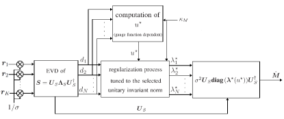
According to Theorem III.3, a unique solution to 𝒫1subscript𝒫1{\cal{P}}_{1} can be constructed in almost closed form. Consequently, this new class of estimators effectively performs specific unitary invariant norm-based projections. It is also worth pointing out that the functional dependence over the selected norm is concentrated in the optimal value of the auxiliary u𝑢u that accounts for the corresponding gauge function. In Fig. 2, a schematic illustration of the steps involved in the proposed procedure for the computation of 𝑴^^𝑴\widehat{\mbox{\boldmath{$M$}}} is reported. As already highlighted, 𝑴^^𝑴\widehat{\mbox{\boldmath{$M$}}} is a shrinkage estimator which regularizes the sample covariance matrix according to the specific unitary invariant norm and explicitly accounting for a condition number constraint so as to provide a well-conditioned structured estimate.
Refer to caption
Figure 2: Block scheme associated with the proposed estimation procedure.

Before continue further, it is worth observing that the functions hi(u)subscript𝑖𝑢h_{i}(u), i=1,,N𝑖1𝑁i=1,\ldots,N, involved in 𝒫3subscript𝒫3{\cal{P}}_{3} can be expressed in closed form666The interested reader may refer to the supplementary material for the proof.. This is a useful result in general and more important it lays the ground for the derivation of specialized procedures to handle 𝒫3subscript𝒫3{\cal{P}}_{3} assuming either the Frobenius or the spectral norm (see Subsections III-A and III-B). Precisely, if di>1subscript𝑑𝑖1d_{i}>1

hi(u)={diκMuif1κMu<diκM0ifdiκMu<diudiifudi,subscript𝑖𝑢casessubscript𝑑𝑖subscript𝜅𝑀𝑢if1subscript𝜅𝑀𝑢subscript𝑑𝑖subscript𝜅𝑀0ifsubscript𝑑𝑖subscript𝜅𝑀𝑢subscript𝑑𝑖𝑢subscript𝑑𝑖if𝑢subscript𝑑𝑖h_{i}(u)=\left\{\begin{array}[c]{ll}d_{i}-\kappa_{M}u&\mbox{if}\quad\frac{1}{\kappa_{M}}\leq u<\frac{d_{i}}{\kappa_{M}}\\ 0&\mbox{if}\quad\frac{d_{i}}{\kappa_{M}}\leq u<d_{i}\\ u-d_{i}&\mbox{if}\quad u\geq d_{i}\\ \end{array}\right., (16)

otherwise di1subscript𝑑𝑖1d_{i}\leq 1 and

hi(u)={1diif1κMu<1udiifu1.subscript𝑖𝑢cases1subscript𝑑𝑖if1subscript𝜅𝑀𝑢1𝑢subscript𝑑𝑖if𝑢1h_{i}(u)=\left\{\begin{array}[c]{ll}1-d_{i}&\mbox{if}\quad\frac{1}{\kappa_{M}}\leq u<1\\ u-d_{i}&\mbox{if}\quad u\geq 1\\ \end{array}\right.. (17)

III-A Frobenius Norm

The gauge function associated with the Frobenius norm is given by

g(h1(u),h2(u),,hN(u))=i=1N(hi(u))2𝑔subscript1𝑢subscript2𝑢subscript𝑁𝑢superscriptsubscript𝑖1𝑁superscriptsubscript𝑖𝑢2g(h_{1}(u),h_{2}(u),\ldots,h_{N}(u))=\sqrt{\displaystyle{\sum_{i=1}^{N}}{(h_{i}(u)})^{2}}

and the problem to solve boils down to

𝒫4{min𝑢G1(u)s.t.u1κM,subscript𝒫4cases𝑢subscript𝐺1𝑢s.t.𝑢1subscript𝜅𝑀{\cal{P}}_{4}\left\{\begin{array}[c]{ll}\underset{u}{\min}&G_{1}(u)\\ \mbox{s.t.}&u\geq\frac{1}{\kappa_{M}}\\ \end{array}\right., (18)

where G1(u)=i=1N(hi(u))2subscript𝐺1𝑢superscriptsubscript𝑖1𝑁superscriptsubscript𝑖𝑢2G_{1}(u)=\displaystyle{\sum_{i=1}^{N}}{(h_{i}(u))^{2}}. To proceed further, let us observe that the optimal solution to problem 𝒫4subscript𝒫4{\cal{P}}_{4} is u=max{1,d1}κMsuperscript𝑢1subscript𝑑1subscript𝜅𝑀u^{\star}=\frac{\max\{1,d_{1}\}}{\kappa_{M}} if d1κMsubscript𝑑1subscript𝜅𝑀d_{1}\leq\kappa_{M}, otherwise, the optimal solution to 𝒫4subscript𝒫4{\cal{P}}_{4} lies within the interval777The interested reader may refer to the supplementary material for the proof. [1,d1]1subscript𝑑1[1,d_{1}]. In this last case, as shown in supplementary material, G1(u)subscript𝐺1𝑢G_{1}(u) is a convex function with a continuous derivative function within the interval of interest [1,d1]1subscript𝑑1\left[1,d_{1}\right]. Hence, denoting by N¯¯𝑁\bar{N} the number of sample eigenvalues disubscript𝑑𝑖d_{i} greater than 111, i.e. di>1subscript𝑑𝑖1d_{i}>1, i=1,,N¯𝑖1¯𝑁i=1,\ldots,\bar{N}, and defining the vector

𝒗=[d1,d2,,dN¯,1]TN¯+1,𝒗superscriptsubscript𝑑1subscript𝑑2subscript𝑑¯𝑁1𝑇superscript¯𝑁1\mbox{\boldmath{$v$}}=\left[d_{1},d_{2},\ldots,d_{\bar{N}},1\right]^{T}\in\mathbb{R}^{\bar{N}+1},

the following theorem holds true.

Theorem III.4

Assuming d1>κM>1subscript𝑑1subscript𝜅𝑀1d_{1}>\kappa_{M}>1, the optimal solution usuperscript𝑢u^{\star} to 𝒫4subscript𝒫4{\cal{P}}_{4} is

  1. 1.

    u=1superscript𝑢1u^{\star}=1, if dG1(u)du|u=10evaluated-at𝑑subscript𝐺1𝑢𝑑𝑢𝑢10\frac{dG_{1}(u)}{du}\Big{|}_{u=1}\geq 0;

  2. 2.

    u=d1superscript𝑢subscript𝑑1u^{\star}=d_{1}, if dG1(u)du|u=d10evaluated-at𝑑subscript𝐺1𝑢𝑑𝑢𝑢subscript𝑑10\frac{dG_{1}(u)}{du}\Big{|}_{u=d_{1}}\leq 0;

  3. 3.

    u=d1κMsuperscript𝑢subscript𝑑1subscript𝜅𝑀u^{\star}=\frac{d_{1}}{\kappa_{M}}, if d1κMdNsubscript𝑑1subscript𝜅𝑀subscript𝑑𝑁\frac{d_{1}}{\kappa_{M}}\leq d_{N};

  4. 4.

    if 1)1), 2)2), and 3)3) are not satisfied, usuperscript𝑢u^{\star} is the optimal solution if and only if

    u=i=1βκMdi+i=αNdiNα+1+βκM2,superscript𝑢superscriptsubscript𝑖1𝛽subscript𝜅𝑀subscript𝑑𝑖superscriptsubscript𝑖𝛼𝑁subscript𝑑𝑖𝑁𝛼1𝛽superscriptsubscript𝜅𝑀2u^{\star}=\frac{\displaystyle{\sum_{i=1}^{\beta}}\kappa_{M}d_{i}+\displaystyle{\sum_{i=\alpha}^{N}}d_{i}}{N-\alpha+1+{\beta}\kappa_{M}^{2}}, (19)

    with α{1,2,,N¯,N¯+1}𝛼12¯𝑁¯𝑁1\alpha\in\{1,2,\ldots,\bar{N},\bar{N}+1\} the smallest index such that vα<usubscript𝑣𝛼superscript𝑢v_{\alpha}<u^{\star}, and β{1,2,,N¯,N¯+1}𝛽12¯𝑁¯𝑁1\beta\in\{1,2,\ldots,\bar{N},\bar{N}+1\} the largest index such that vβκM>usubscript𝑣𝛽subscript𝜅𝑀superscript𝑢\frac{v_{\beta}}{\kappa_{M}}>u^{\star}.

Proof:

See Appendix -D. ∎

Theorem III.4 provides the guidelines to find usuperscript𝑢u^{\star}. Indeed, the selection of the integers α𝛼\alpha and β𝛽\beta such that

uα,β=i=1βκMdi+i=αNdiNα+1+βκM2,subscript𝑢𝛼𝛽superscriptsubscript𝑖1𝛽subscript𝜅𝑀subscript𝑑𝑖superscriptsubscript𝑖𝛼𝑁subscript𝑑𝑖𝑁𝛼1𝛽superscriptsubscript𝜅𝑀2u_{\alpha,\beta}=\frac{\displaystyle{\sum_{i=1}^{\beta}}\kappa_{M}d_{i}+\displaystyle{\sum_{i=\alpha}^{N}}d_{i}}{N-\alpha+1+\beta\kappa_{M}^{2}}, (20)

with

vα<uα,βvα1andvβ+1κMuα,β<vβκM,formulae-sequencesubscript𝑣𝛼subscript𝑢𝛼𝛽subscript𝑣𝛼1andsubscript𝑣𝛽1subscript𝜅𝑀subscript𝑢𝛼𝛽subscript𝑣𝛽subscript𝜅𝑀v_{\alpha}<u_{\alpha,\beta}\leq v_{\alpha-1}\quad\mbox{and}\quad\frac{v_{\beta+1}}{\kappa_{M}}\leq u_{\alpha,\beta}<\frac{v_{\beta}}{\kappa_{M}}, (21)

is required. To this end, an efficient procedure is now described. Precisely, the strategy consists in iteratively verifying the conditions (20) and (21) once the values of α𝛼\alpha and β𝛽\beta have been efficiently fixed. In this respect, notice that, if the intersection of the intervals (21) is empty, then uα,βsubscript𝑢𝛼𝛽u_{\alpha,\beta} cannot be the optimal solution. On the contrary, the intersection is given by one of the following sub-intervals ]vα,vα1],]vα,vβκM[,[vβ+1κM,vα1],[vβ+1κM,vβκM[\Big{]}v_{\alpha},v_{\alpha-1}\Big{]},\left]v_{\alpha},\frac{v_{\beta}}{\kappa_{M}}\right[,\left[\frac{v_{\beta+1}}{\kappa_{M}},v_{\alpha-1}\right],\left[\frac{v_{\beta+1}}{\kappa_{M}},\frac{v_{\beta}}{\kappa_{M}}\right[, and the optimal point must belong to one of them. According to this line of reasoning, the procedure follows these simple steps:

  1. 1.

    Set β=1𝛽1\beta=1, α=2𝛼2\alpha=2, and increase α𝛼\alpha until vαvβκMsubscript𝑣𝛼subscript𝑣𝛽subscript𝜅𝑀v_{\alpha}\geq\frac{v_{\beta}}{\kappa_{M}}.

  2. 2.

    Compute uα,βsubscript𝑢𝛼𝛽u_{\alpha,\beta}. If uα,βsubscript𝑢𝛼𝛽u_{\alpha,\beta} belongs to the current intersection, let u=uα,βsuperscript𝑢subscript𝑢𝛼𝛽u^{\star}=u_{\alpha,\beta} and exit; otherwise go to step 3)3).

  3. 3.

    If vβ+1κM<vαsubscript𝑣𝛽1subscript𝜅𝑀subscript𝑣𝛼\frac{v_{\beta+1}}{\kappa_{M}}<v_{\alpha}, increase α𝛼\alpha and go to step 2)2), otherwise increase β𝛽\beta and go to step 2)2).

It is worth pointing out that this algorithm provides the optimal solution to problem 𝒫4subscript𝒫4{\cal{P}}_{4} with a linear computational complexity with the number of the sample covariance matrix eigenvalues greater than 111.

III-B Spectral Norm

In this case, the gauge function is

g(h1(u),h2(u),,hN(u))=maxi=1,,N{hi(u)}𝑔subscript1𝑢subscript2𝑢subscript𝑁𝑢subscript𝑖1𝑁subscript𝑖𝑢g(h_{1}(u),h_{2}(u),\ldots,h_{N}(u))=\displaystyle{\max_{i=1,\ldots,N}}\left\{{h_{i}(u)}\right\}

and 𝒫3subscript𝒫3{\cal{P}}_{3} can be specialized as

𝒫¯3{min𝑢G2(u)s.t.u1κM,subscript¯𝒫3cases𝑢subscript𝐺2𝑢s.t.𝑢1subscript𝜅𝑀\bar{{\cal{P}}}_{3}\left\{\begin{array}[c]{ll}\underset{u}{\min}&G_{2}(u)\\ \mbox{s.t.}&u\geq\frac{1}{\kappa_{M}}\\ \end{array}\right., (22)

with G2(u)=max𝑖{hi(u)}subscript𝐺2𝑢𝑖subscript𝑖𝑢G_{2}(u)=\underset{i}{\max}\left\{h_{i}(u)\right\}.

The following proposition provides an efficient procedure to solve 𝒫¯3subscript¯𝒫3\bar{{\cal{P}}}_{3}.

Theorem III.5

Let usuperscript𝑢u^{\star} the lowest optimal solution to 𝒫¯3subscript¯𝒫3\bar{{\cal{P}}}_{3}. Then

  1. 1.

    u=1κMsuperscript𝑢1subscript𝜅𝑀u^{\star}=\frac{1}{\kappa_{M}}, if d11subscript𝑑11d_{1}\leq 1.

  2. 2.

    u=max{d1+dN1κM,1κM}superscript𝑢subscript𝑑1subscript𝑑𝑁1subscript𝜅𝑀1subscript𝜅𝑀u^{\star}=\max\left\{\frac{d_{1}+d_{N}-1}{\kappa_{M}},\frac{1}{\kappa_{M}}\right\}, if 1<d1κM1subscript𝑑1subscript𝜅𝑀1<d_{1}\leq\kappa_{M} and dN1subscript𝑑𝑁1d_{N}\leq 1.

  3. 3.

    u=d1κMsuperscript𝑢subscript𝑑1subscript𝜅𝑀u^{\star}=\frac{d_{1}}{\kappa_{M}}, if 1<d1κM1subscript𝑑1subscript𝜅𝑀1<d_{1}\leq\kappa_{M} and dN>1subscript𝑑𝑁1d_{N}>1. In this case, the covariance estimate reduces to 𝐒𝐒S.

  4. 4.

    If d1>κMsubscript𝑑1subscript𝜅𝑀d_{1}>\kappa_{M} and dN1subscript𝑑𝑁1d_{N}\leq 1, then

    • u=max{η1,1κM}superscript𝑢subscript𝜂11subscript𝜅𝑀u^{\star}=\max\left\{\eta_{1},\frac{1}{\kappa_{M}}\right\}, if η1=d1+dN1κM1subscript𝜂1subscript𝑑1subscript𝑑𝑁1subscript𝜅𝑀1\eta_{1}=\frac{d_{1}+d_{N}-1}{\kappa_{M}}\leq 1;

    • otherwise, u=d1+dN1+κM>1superscript𝑢subscript𝑑1subscript𝑑𝑁1subscript𝜅𝑀1u^{\star}=\frac{d_{1}+d_{N}}{1+\kappa_{M}}>1.

  5. 5.

    If d1>κMsubscript𝑑1subscript𝜅𝑀d_{1}>\kappa_{M} and dN>1subscript𝑑𝑁1d_{N}>1, then

    • u=d1+dN1+κMsuperscript𝑢subscript𝑑1subscript𝑑𝑁1subscript𝜅𝑀u^{\star}=\frac{d_{1}+d_{N}}{1+\kappa_{M}}. if dNd1κMsubscript𝑑𝑁subscript𝑑1subscript𝜅𝑀d_{N}\leq\frac{d_{1}}{\kappa_{M}};

    • otherwise, u=d1κMsuperscript𝑢subscript𝑑1subscript𝜅𝑀u^{\star}=\frac{d_{1}}{\kappa_{M}}. Besides, in this case, the estimate coincides with 𝐒𝐒S.

Proof:

See Appendix -E. ∎

Based on Theorem III.5, the optimal solution to 𝒫¯3subscript¯𝒫3\bar{{\cal{P}}}_{3} is substantially available in closed form. Indeed, just the comparison between some linear functions of the highest and the lowest sample covariance eigenvalues with some fixed thresholds is required. It is also worth pointing out that, usuperscript𝑢u^{\star} is a continuous function of d1,,dNsubscript𝑑1subscript𝑑𝑁d_{1},\ldots,d_{N} implying that 𝑿superscript𝑿\mbox{\boldmath{$X$}}^{\star} is a continuous function of 𝑺𝑺S.

IV Performance Analysis

This section is devoted to the analysis of the proposed covariance estimators. The average SINR is adopted as performance metric and some counterparts available in the open literature are considered for comparison purposes. Two typical radar signal processing scenarios are studied: the former focuses on spatial processing with wideband jammers impairing the received data, the latter considers Doppler processing with the interfering returns originated by clutter. More formally, the average SINR (over MC𝑀𝐶MC i.i.d. realizations888In the numerical results the number of Monte Carlo trials is set to MC=500𝑀𝐶500MC=500. of K𝐾K secondary data) is given by

SINRav=1MCi=1MC|𝒘^i𝒔(x)|2(𝒘^i𝑴𝒘^i),subscriptSINR𝑎𝑣1𝑀𝐶superscriptsubscript𝑖1𝑀𝐶superscriptsuperscriptsubscript^𝒘𝑖𝒔𝑥2superscriptsubscript^𝒘𝑖𝑴subscript^𝒘𝑖\mbox{SINR}_{av}=\frac{1}{MC}\sum_{i=1}^{MC}\frac{|\widehat{\mbox{\boldmath{$w$}}}_{i}^{{\dagger}}\mbox{\boldmath{$s$}}(x)|^{2}}{\left(\widehat{\mbox{\boldmath{$w$}}}_{i}^{{\dagger}}\mbox{\boldmath{$M$}}\widehat{\mbox{\boldmath{$w$}}}_{i}\right)}, (23)

where 𝒔(x)𝒔𝑥\mbox{\boldmath{$s$}}(x) is the N𝑁N-dimensional target steering vector whose expression depends on:

  • the considered processing scenario (spatial/temporal);

  • the radar configuration (array type, Pulse Repetition Time (PRT), etc.);

  • the target state x𝑥x (angle of arrival θ𝜃\theta/normalized Doppler frequency ν𝜈\nu).

Moreover, 𝒘^i=𝑴^i1𝒔(x)subscript^𝒘𝑖superscriptsubscript^𝑴𝑖1𝒔𝑥\widehat{\mbox{\boldmath{$w$}}}_{i}=\widehat{\mbox{\boldmath{$M$}}}_{i}^{-1}\mbox{\boldmath{$s$}}(x) is the adaptive estimate of the optimal weight vector, where 𝑴^isubscript^𝑴𝑖\widehat{\mbox{\boldmath{$M$}}}_{i} is the data-dependent estimate of 𝑴𝑴M at the i𝑖i-th run.

In the following analysis, it is assumed σ2=0superscript𝜎20\sigma^{2}=0 dB and κM=λmax(𝑴)/λmin(𝑴)subscript𝜅𝑀subscript𝜆𝑚𝑎𝑥𝑴subscript𝜆𝑚𝑖𝑛𝑴\kappa_{M}=\lambda_{max}(\mbox{\boldmath{$M$}})/\lambda_{min}(\mbox{\boldmath{$M$}}). Furthermore, for each case study two different values of the actual white noise power level are considered, i.e., σa2=0superscriptsubscript𝜎𝑎20\sigma_{a}^{2}=0 and σa2=10superscriptsubscript𝜎𝑎210\sigma_{a}^{2}=10 dB, so as to account for both a matched and a mismatched scenario.

IV-A Spatial Processing

A radar system equipped with a uniform linear array of N=8𝑁8N=8 elements (with a spacing between the antennas of d=λ0/2𝑑subscript𝜆02d=\lambda_{0}/2 where λ0subscript𝜆0\lambda_{0} is the radar operating wavelength) pointing in the boresight direction is considered. The interference covariance matrix is given by 𝑴=𝑴s+σa2𝑰𝑴subscript𝑴𝑠superscriptsubscript𝜎𝑎2𝑰\mbox{\boldmath{$M$}}=\mbox{\boldmath{$M$}}_{s}+\sigma_{a}^{2}\mbox{\boldmath{$I$}} [9] where σa2superscriptsubscript𝜎𝑎2\sigma_{a}^{2} is the actual power level of the white disturbance term, whereas 𝑴ssubscript𝑴𝑠\mbox{\boldmath{$M$}}_{s} is the covariance matrix associated to J𝐽J (possibly wideband) jammers. Specifically, (n,m){1,,N}2for-all𝑛𝑚superscript1𝑁2\forall\left(n,m\right)\in\left\{1,\ldots,N\right\}^{2},

𝑴s(n,m)=i=1Jσi2sinc[0.5Bf(nm)ϕi]ej(nm)ϕi,subscript𝑴𝑠𝑛𝑚superscriptsubscript𝑖1𝐽superscriptsubscript𝜎𝑖2sincdelimited-[]0.5subscript𝐵𝑓𝑛𝑚subscriptitalic-ϕ𝑖superscript𝑒𝑗𝑛𝑚subscriptitalic-ϕ𝑖\begin{split}\mbox{\boldmath{$M$}}_{s}\left(n,m\right)=\displaystyle{\sum_{i=1}^{J}}&\sigma_{i}^{2}\mbox{sinc}\left[0.5B_{f}(n-m)\phi_{i}\right]e^{j(n-m)\phi_{i}},\\ \end{split} (24)

with Bf=B/f0subscript𝐵𝑓𝐵subscript𝑓0B_{f}=B/f_{0} the fractional bandwidth, B𝐵B the instantaneous bandwidth of the desired signal (coinciding with the jammer’s bandwidth), f0=c/λ0subscript𝑓0𝑐subscript𝜆0f_{0}=c/\lambda_{0}, σi2superscriptsubscript𝜎𝑖2\sigma_{i}^{2} the power associated with the i𝑖i-th jammer, and ϕisubscriptitalic-ϕ𝑖\phi_{i} the jammer phase angle with respect to the antenna phase center. Precisely, ϕi=2πd(sinθi)/λ0subscriptitalic-ϕ𝑖2𝜋𝑑subscript𝜃𝑖subscript𝜆0\phi_{i}=2\pi d(\sin\theta_{i})/\lambda_{0}, with θisubscript𝜃𝑖\theta_{i} the angle off-boresight of the jammer. Finally, according to the specified system model, the steering vector (23) reduces to

𝒔(θ)=[1,exp(jπsin(θ)),,exp(jπsin(θ)(N1))]T.𝒔𝜃superscript1𝑗𝜋𝜃𝑗𝜋𝜃𝑁1𝑇\mbox{\boldmath{$s$}}(\theta)=\left[1,\exp\left(j\pi\sin(\theta)\right),\ldots,\exp\left(j\pi\sin(\theta)(N-1)\right)\right]^{T}.

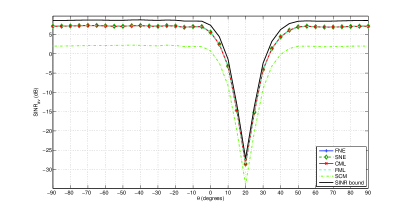
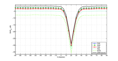
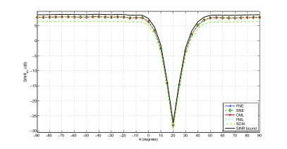
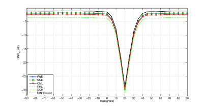
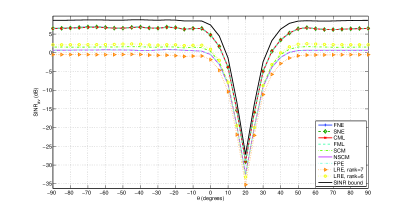
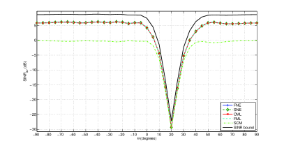
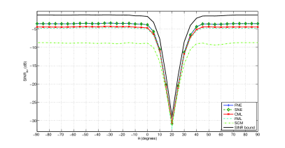
As case study, it is considered a wideband jammer with a fractional bandwidth Bf1=0.3subscript𝐵subscript𝑓10.3B_{f_{1}}=0.3, a power σ12=30superscriptsubscript𝜎1230\sigma_{1}^{2}=30 dB, and a direction of arrival θ1=20subscript𝜃120\theta_{1}=20 deg that impinges of the radar receive array. In Fig. 3, the average SINR is plotted versus the Direction Of Arrival (DOA) θ𝜃\theta for both the Frobenius Norm based Estimator (FNE) and the Spectral Norm based Estimator (SNE). Therein, the secondary data are modeled as i.i.d., zero-mean, circularly symmetric Gaussian random vectors. For comparison purposes, the SINR behavior associated with the Constrained ML estimator (CML) [11], the Fast Maximum Likelihood estimator (FML) [9], and the classic Sample Covariance Matrix (SCM)999Notice that, when K<N𝐾𝑁K<N the pseudo inverse of the sample matrix is utilized in place of its inverse [1]. is displayed too. Besides, the SINR upper bound 𝒔𝑴1𝒔superscript𝒔superscript𝑴1𝒔\mbox{\boldmath{$s$}}^{{\dagger}}\mbox{\boldmath{$M$}}^{-1}\mbox{\boldmath{$s$}} is reported as benchmark. Figs. 3(a), 3(c), 3(e) assume a matched condition, i.e. σa2=σ2=0superscriptsubscript𝜎𝑎2superscript𝜎20\sigma_{a}^{2}=\sigma^{2}=0 dB, with K=4𝐾4K=4, K=8𝐾8K=8, and K=16𝐾16K=16 secondary data, respectively. Figs. 3(b), 3(d), 3(e) account for a mismatched situation, i.e. σa2=10superscriptsubscript𝜎𝑎210\sigma_{a}^{2}=10 dB and σ2=0superscript𝜎20\sigma^{2}=0 dB.

The results show that FNE and SNE substantially exhibit the same performance in terms of average SINR regardless of the considered DOA and scenario. In the matched cases the curves of the new devised estimators almost overlap with those of FML and CML (the maximum gain of FNE and SNE over CML and FML is 0.08 dB) and significantly dominate the SCM performance. Besides, FNE and SNE outperform all the counterparts in the mismatched scenario with gains (with respect to CML, FML, and SCM) of: 0.930.930.93 dB, 1.261.261.26 dB, and 5.655.655.65 dB for K=4𝐾4K=4; 0.800.800.80 dB, 2.402.402.40 dB, and 5.455.455.45 dB for K=8𝐾8K=8; 0.450.450.45 dB, 1.601.601.60 dB, and 1.601.601.60 dB for K=16𝐾16K=16. As expected, increasing the sample support size the gain reduces since all the curves tend to approach the SINR upper bound due to the consistency of the estimators.
Refer to caption
(a) σa2=0superscriptsubscript𝜎𝑎20\sigma_{a}^{2}=0 dB, K=4𝐾4K=4
Refer to caption
(b) σa2=10superscriptsubscript𝜎𝑎210\sigma_{a}^{2}=10 dB, K=4𝐾4K=4
Refer to caption
(c) σa2=0superscriptsubscript𝜎𝑎20\sigma_{a}^{2}=0 dB, K=8𝐾8K=8
Refer to caption
(d) σa2=10superscriptsubscript𝜎𝑎210\sigma_{a}^{2}=10 dB, K=8𝐾8K=8
Refer to caption
(e) σa2=0superscriptsubscript𝜎𝑎20\sigma_{a}^{2}=0 dB, K=16𝐾16K=16
Refer to caption
(f) σa2=10superscriptsubscript𝜎𝑎210\sigma_{a}^{2}=10 dB, K=16𝐾16K=16
Figure 3: Spatial processing in the presence of Gaussian secondary data for different numbers of training data. SINRavsubscriptSINR𝑎𝑣\mbox{SINR}_{av} versus θ𝜃\theta (blue curve ++-marked FNE, green dashed curve SNE, red ×\times-marked curve CML, cyan dashed curve FML, green dot-dashed curve SCM, and the black curve ideal SINR bound). A wideband jammer with Bf1=0.3subscript𝐵subscript𝑓10.3B_{f_{1}}=0.3, σ12=30subscriptsuperscript𝜎2130\sigma^{2}_{1}=30 dB and θ1=20subscript𝜃120\theta_{1}=20 deg is present. Subplots (a), (c), and (e) refer to the case σa2=0superscriptsubscript𝜎𝑎20\sigma_{a}^{2}=0 dB, whereas subplots (b), (d), and (f) to σa2=10superscriptsubscript𝜎𝑎210\sigma_{a}^{2}=10 dB.

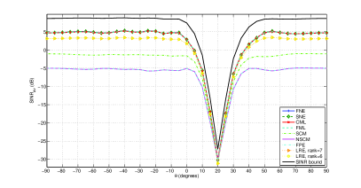
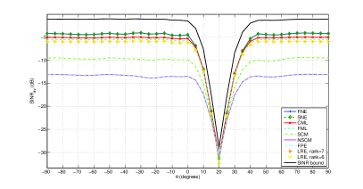
In Fig. 4, the same spatial processing scenario as in Fig. 3 is analyzed, but for a different secondary data statistical distribution that is no longer Gaussian. Specifically,

𝒓i=𝒏i+τi𝒙ii=1,,K,formulae-sequencesubscript𝒓𝑖subscript𝒏𝑖subscript𝜏𝑖subscript𝒙𝑖𝑖1𝐾\mbox{\boldmath{$r$}}_{i}=\mbox{\boldmath{$n$}}_{i}+\sqrt{\tau_{i}}\mbox{\boldmath{$x$}}_{i}\,\quad i=1,\ldots,K,

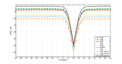
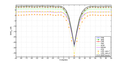
where 𝒏i𝒞𝒩(0,σa2𝑰)similar-tosubscript𝒏𝑖𝒞𝒩0superscriptsubscript𝜎𝑎2𝑰\mbox{\boldmath{$n$}}_{i}\sim\mathcal{CN}(0,\sigma_{a}^{2}\mbox{\boldmath{$I$}}), 𝒙i𝒞𝒩(0,𝑴s)similar-tosubscript𝒙𝑖𝒞𝒩0subscript𝑴𝑠\mbox{\boldmath{$x$}}_{i}\sim\mathcal{CN}(0,\mbox{\boldmath{$M$}}_{s}), and τiΓ(1/μτ,μτ)similar-tosubscript𝜏𝑖Γ1subscript𝜇𝜏subscript𝜇𝜏\tau_{i}\sim\Gamma(1/\mu_{\tau},\mu_{\tau}) (μτ=2subscript𝜇𝜏2\mu_{\tau}=2), i=1,,K𝑖1𝐾i=1,\ldots,K, are statistically independent random variables/vectors. Otherwise stated, a compound Gaussian jamming is now accounted for. As in Fig. 3, the average SINR versus θ𝜃\theta is reported for three different sample support sizes, i.e., K=4𝐾4K=4, K=8𝐾8K=8, and K=16𝐾16K=16. Moreover, the subplots on the left refer to the matched scenario (σa2=σ2=0superscriptsubscript𝜎𝑎2superscript𝜎20\sigma_{a}^{2}=\sigma^{2}=0 dB) whereas the plot on the right address the mismatched case (σa2=10superscriptsubscript𝜎𝑎210\sigma_{a}^{2}=10 dB and σ2=0superscript𝜎20\sigma^{2}=0 dB).

For comparison purposes, other than the FML, CML, and SCM estimators, three additional strategies designed to operate in compound Gaussian clutter are considered. Specifically,

  • the Normalized Sample Covariance Matrix estimator (NSCM), [43]

    𝑴^NSCM=NKi=1K𝒓i𝒓i𝒓i𝒓i;subscript^𝑴NSCM𝑁𝐾superscriptsubscript𝑖1𝐾subscript𝒓𝑖superscriptsubscript𝒓𝑖superscriptsubscript𝒓𝑖subscript𝒓𝑖\widehat{\mbox{\boldmath{$M$}}}_{\text{NSCM}}=\frac{N}{K}\sum_{i=1}^{K}\frac{\mbox{\boldmath{$r$}}_{i}\mbox{\boldmath{$r$}}_{i}^{{\dagger}}}{\mbox{\boldmath{$r$}}_{i}^{{\dagger}}\mbox{\boldmath{$r$}}_{i}};
  • the Fixed-Point Estimator (FPE) [44, 45, 46] 𝑴^FPEsubscript^𝑴FPE\widehat{\mbox{\boldmath{$M$}}}_{\text{FPE}}, that is obtained iteratively solving a fixed point equation;

  • the Low Rank clutter Estimator (LRE), [17], addressing a mixed Gaussian/compound Gaussian disturbance model. The covariance estimate can be computed as

    𝑴^LRE=(1Kk=1Kτ^k)𝚺^+𝑰,subscript^𝑴LRE1𝐾superscriptsubscript𝑘1𝐾subscript^𝜏𝑘^𝚺𝑰\widehat{\mbox{\boldmath{$M$}}}_{\text{LRE}}=\left(\frac{1}{K}\sum_{k=1}^{K}\widehat{\tau}_{k}\right)\widehat{\mbox{\boldmath{$\Sigma$}}}+\mbox{\boldmath{$I$}},

    where τ^ksubscript^𝜏𝑘\widehat{\tau}_{k} is the estimated texture of the k𝑘k-th clutter datum and 𝚺^^𝚺\widehat{\mbox{\boldmath{$\Sigma$}}} is the covariance estimate of the speckle obtained through the iterative algorithm proposed in [17].

Inspection of Fig. 4 reveals that FNE and SNE are basically equivalent and outperform in terms of average SINR all the counterparts, included those specific for compound Gaussian disturbance101010As to the LRE, the clutter covariance matrix rank is evaluated as the number of the eigenvalues greater than tr(𝑴s)/105104trsubscript𝑴𝑠superscript105superscript104\mbox{\rm tr}\,(\mbox{\boldmath{$M$}}_{s})/10^{5}\geq 10^{-4}. Hence, the estimators exploiting the true rank, i.e., 6 (LRE-6) and rank 7 (LRE-7) are displayed.. Precisely, in the matched condition, as already observed in Fig. 3, FNE, SNE, FML, and CML are almost coincident. Besides, compared to NSCM, FPE, LRE-6, LRE-7, and SCM, they provide SINR gains up to: 111111 dB, 111111 dB, 1.891.891.89 dB, 1.901.901.90 dB, and 6.936.936.93 dB for K=4𝐾4K=4; 6.276.276.27 dB, 6.276.276.27 dB, 4.744.744.74 dB, 7.507.507.50 dB, and 5.385.385.38 dB for K=8𝐾8K=8; 4.774.774.77 dB, 2.012.012.01 dB, 6.656.656.65 dB, 9.209.209.20 dB, 1.631.631.63 dB for K=16𝐾16K=16. Without surprise, LRE-6 outperforms LRE-7 reflecting the presence of a mismatch loss. Finally, in the mismatched scenario, FNE and SNE also grant better performance than FML and CML with gains of 1.351.351.35 dB and 0.940.940.94 dB for K=4𝐾4K=4, 2.352.352.35 dB and 0.840.840.84 dB, for K=8𝐾8K=8, 1.511.511.51 dB and 0.420.420.42 dB, for K=16𝐾16K=16, clearly highlighting the effectiveness of the new devised strategies. As to the comparisons with the other estimators, considerations similar to those for the matched scenario holds true.
Refer to caption
(a) σa2=0superscriptsubscript𝜎𝑎20\sigma_{a}^{2}=0 dB, K=4𝐾4K=4
Refer to caption
(b) σa2=10superscriptsubscript𝜎𝑎210\sigma_{a}^{2}=10 dB, K=4𝐾4K=4
Refer to caption
(c) σa2=0superscriptsubscript𝜎𝑎20\sigma_{a}^{2}=0 dB, K=8𝐾8K=8
Refer to caption
(d) σa2=10superscriptsubscript𝜎𝑎210\sigma_{a}^{2}=10 dB, K=8𝐾8K=8
Refer to caption
(e) σa2=0superscriptsubscript𝜎𝑎20\sigma_{a}^{2}=0 dB, K=16𝐾16K=16
Refer to caption
(f) σa2=10superscriptsubscript𝜎𝑎210\sigma_{a}^{2}=10 dB, K=16𝐾16K=16
Figure 4: Spatial processing in the presence of mixed Gaussian and compound Gaussian data. SINRavsubscriptSINR𝑎𝑣\mbox{SINR}_{av} versus θ𝜃\theta (blue curve ++-marked FNE, green dashed curve SNE, red ×\times-marked curve CML, cyan dashed curve FML, green dot-dashed curve SCM, magenta curve NSCM, cyan dot-dashed curve FPE, orange dotted curve \triangleright-marked LRE-7 , yellow dotted curve \circ-marked LRE-6, and black curve ideal SINR bound). A wideband jammer with Bf1=0.3subscript𝐵subscript𝑓10.3B_{f_{1}}=0.3, σ12=30subscriptsuperscript𝜎2130\sigma^{2}_{1}=30 dB and θ1=20subscript𝜃120\theta_{1}=20 deg is present. Subplots (a), (c), and (e) refer to the case σa2=0superscriptsubscript𝜎𝑎20\sigma_{a}^{2}=0 dB, whereas subplots (b), (d), and (f) to σa2=10superscriptsubscript𝜎𝑎210\sigma_{a}^{2}=10 dB.

IV-B Doppler Processing

A radar system transmitting a coherent burst of N=16𝑁16N=16 pulses is considered. In this case x𝑥x refers to the normalized Doppler frequency of the target, i.e. ν[1/2,1/2[\nu\in[-1/2,1/2[ and the steering vector in (23) reduces to

𝒔(ν)=[1,exp(j2πν),,exp(j2πν(N1))]TN.𝒔𝜈superscript1𝑗2𝜋𝜈𝑗2𝜋𝜈𝑁1𝑇superscript𝑁\displaystyle\mbox{\boldmath{$s$}}(\nu)=\left[1,\exp\left(j2\pi\nu\right),\ldots,\exp\left(j2\pi\nu(N-1)\right)\right]^{T}\in\mathbb{C}^{N}.

As to the interference environment, it is assumed that the radar operates in the presence of both ground and sea clutter in addition to white noise [47]. Therefore the overall disturbance covariance matrix is

𝑴=𝑴t+σa2𝑰,𝑴subscript𝑴𝑡superscriptsubscript𝜎𝑎2𝑰\mbox{\boldmath{$M$}}=\mbox{\boldmath{$M$}}_{t}+\sigma_{a}^{2}\mbox{\boldmath{$I$}}, (25)

where, (n,m){1,,N}2for-all𝑛𝑚superscript1𝑁2\forall\left(n,m\right)\in\left\{1,\ldots,N\right\}^{2},

𝑴t(n,m)=CNRSρS(nm)2ej2π(nm)fS+CNRGρG|nm|,subscript𝑴𝑡𝑛𝑚subscriptCNR𝑆superscriptsubscript𝜌𝑆superscript𝑛𝑚2superscript𝑒𝑗2𝜋𝑛𝑚subscript𝑓𝑆subscriptCNR𝐺superscriptsubscript𝜌𝐺𝑛𝑚\begin{split}\mbox{\boldmath{$M$}}_{t}(n,m)=&\text{CNR}_{S}\rho_{S}^{(n-m)^{2}}e^{j2\pi(n-m)f_{S}}+\text{CNR}_{G}\rho_{G}^{|n-m|},\\ \end{split} (26)

with

  • CNRSsubscriptCNR𝑆\text{CNR}_{S} and CNRGsubscriptCNR𝐺\text{CNR}_{G} the power of the sea and ground clutter, respectively;

  • ρSsubscript𝜌𝑆\rho_{S} and ρGsubscript𝜌𝐺\rho_{G} the one-lag correlation coefficients of the sea and the ground clutter, respectively;

  • fSsubscript𝑓𝑆f_{S} the normalized Doppler frequency of the sea clutter.

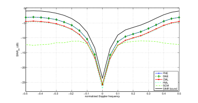
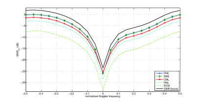
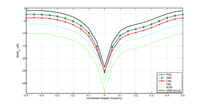
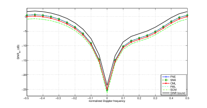
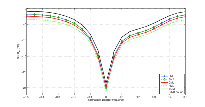
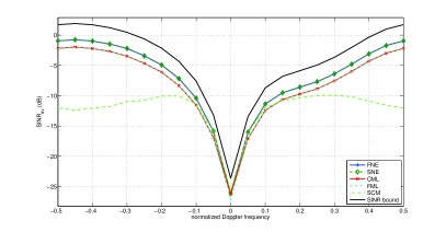
In Fig. 5, the average SINR versus ν𝜈\nu is reported for FNE, SNE, FML, CML, and SCM estimators. The training data are drawn from a complex circular Gaussian distribution and the parameters in (26) are CNRS=10subscriptCNR𝑆10\text{CNR}_{S}=10 dB, CNRG=25subscriptCNR𝐺25\text{CNR}_{G}=25 dB, ρS=0.8subscript𝜌𝑆0.8\rho_{S}=0.8, ρG=0.95subscript𝜌𝐺0.95\rho_{G}=0.95, and fS=0.2subscript𝑓𝑆0.2f_{S}=0.2. Figs. 5(a), 5(c), and 5(e) refer to K=8𝐾8K=8, K=16𝐾16K=16, and K=32𝐾32K=32, respectively and assume σa2=0superscriptsubscript𝜎𝑎20\sigma_{a}^{2}=0 dB. The mismatched analysis, i.e., σa2=10superscriptsubscript𝜎𝑎210\sigma_{a}^{2}=10 dB, is instead reported in Figs. 5(b), 5(d), and 5(f).

The plots clearly illustrate the effectiveness of the new devised estimators. Indeed, both in the matched and in mismatched scenario, FNE and SNE achieve higher SINR values than the counterparts at each target Doppler frequency. Interestingly, unlike the spatial-processing, in this case FNE and SNE also outperform CML and FML in the matched conditions. Precisely, the SINR gains with respect to the CML, that is the major competitor, are, for K=8,16,32𝐾81632K=8,16,32, respectively: 1.291.291.29 dB, 1.381.381.38 dB, and 0.520.520.52 dB in the matched case and 1.431.431.43 dB, 1.421.421.42 dB, and 0.610.610.61 dB in mismatched situation. As expected, the gains are lower and lower as K𝐾K increases, due to the consistency of all the involved estimators.
Refer to caption
(a) σa2=0superscriptsubscript𝜎𝑎20\sigma_{a}^{2}=0 dB, K=8𝐾8K=8
Refer to caption
(b) σa2=10superscriptsubscript𝜎𝑎210\sigma_{a}^{2}=10 dB, K=8𝐾8K=8
Refer to caption
(c) σa2=0superscriptsubscript𝜎𝑎20\sigma_{a}^{2}=0 dB, K=16𝐾16K=16
Refer to caption
(d) σa2=10superscriptsubscript𝜎𝑎210\sigma_{a}^{2}=10 dB, K=16𝐾16K=16
Refer to caption
(e) σa2=0superscriptsubscript𝜎𝑎20\sigma_{a}^{2}=0 dB, K=32𝐾32K=32
Refer to caption
(f) σa2=10superscriptsubscript𝜎𝑎210\sigma_{a}^{2}=10 dB, K=32𝐾32K=32
Figure 5: Doppler processing in the presence of Gaussian data for different numbers of training data. SINRavsubscriptSINR𝑎𝑣\mbox{SINR}_{av} versus normalized Doppler frequency (blue curve ++-marked FNE, green dashed curve SNE, red ×\times-marked curve CML, cyan dashed curve FML, green dot-dashed curve SCM, and black curve ideal SINR bound). The analyzed environment comprises a bimodal clutter composed of sea and ground clutter with CNRS=10subscriptCNR𝑆10\text{CNR}_{S}=10 dB, CNRG=25subscriptCNR𝐺25\text{CNR}_{G}=25, ρS=0.8subscript𝜌𝑆0.8\rho_{S}=0.8, ρG=0.95subscript𝜌𝐺0.95\rho_{G}=0.95, and fS=0.2subscript𝑓𝑆0.2f_{S}=0.2. Subplots (a), (c), and (e) refer to the case σa2=0superscriptsubscript𝜎𝑎20\sigma_{a}^{2}=0 dB, whereas subplots (b), (d), and (f) to σa2=10superscriptsubscript𝜎𝑎210\sigma_{a}^{2}=10 dB.

V Conclusions

The disturbance covariance matrix estimation problem for radar signal processing applications has been addressed according to a geometric approach. Specifically, a new family of distribution-free covariance estimators has been introduced performing the sample covariance matrix projection, according to a specific unitary invariant norm, into a structured covariance set of practical relevance.

To tackle the resulting constrained optimization problem an efficient solution technique has been designed which represents the main technical contribution of this paper. In particular, it has been proved that each estimator exhibits a shrinkage-type form with the eigenvalues estimate obtained via the solution of a one-dimensional convex problem tuned to the considered unitary norm. Furthermore, almost closed form covariance estimates have been provided assuming either Frobenius or spectral norms at the design stage. Remarkably, the proposed estimators possess the consistency property as long as the training vectors are statistically independent.

Some interesting case studies have been considered to illustrate the effectiveness of the new proposed framework. The results have shown that the new estimators may provide better SINR values than some structured estimators available in the open literature. Precisely, the lower the sample support the higher the gain. Additionally, accounting for the computational efforts as well as the SINR performance, the best estimator appears that based on spectral norm.

As possible future research tracks, it might be worth analyzing the performance of the new family of estimators on real radar data as well as to account for other unitary invariant constraint at the design stage such as an upper bound on the clutter rank.

-A Proof of Lemma III.1

Proof:

Let 𝑿1=𝑼1𝚲1𝑼1superscriptsubscript𝑿1subscript𝑼1superscriptsubscript𝚲1subscriptsuperscript𝑼1{\mbox{\boldmath{$X$}}}_{1}^{\star}={\mbox{\boldmath{$U$}}}_{1}{\mbox{\boldmath{$\Lambda$}}}_{1}^{\star}{\mbox{\boldmath{$U$}}}^{{\dagger}}_{1} be the spectral decomposition of an optimal solution to 𝒫1subscript𝒫1{\cal{P}}_{1}, where 𝚲1=diag(λ1,λ2,,λN)superscriptsubscript𝚲1diagsuperscriptsubscript𝜆1superscriptsubscript𝜆2superscriptsubscript𝜆𝑁{\mbox{\boldmath{$\Lambda$}}}_{1}^{\star}=\mbox{\boldmath\bf diag}\,(\lambda_{1}^{\star},\lambda_{2}^{\star},\cdots,\lambda_{N}^{\star}), with λ1λ2λNsuperscriptsubscript𝜆1superscriptsubscript𝜆2superscriptsubscript𝜆𝑁\lambda_{1}^{\star}\geq\lambda_{2}^{\star}\geq\cdots\geq\lambda_{N}^{\star}. Based on [39, Theorem 7.4.51]

𝑿1𝑺𝚲1𝚲S.normsuperscriptsubscript𝑿1𝑺normsuperscriptsubscript𝚲1subscript𝚲𝑆\|{\mbox{\boldmath{$X$}}}_{1}^{\star}-\mbox{\boldmath{$S$}}\|\geq\|{\mbox{\boldmath{$\Lambda$}}}_{1}^{\star}-{\mbox{\boldmath{$\Lambda$}}}_{S}\|. (27)

Besides,

𝚲1𝚲S=𝑼S(𝚲1𝚲S)𝑼S=𝑿𝑺,normsuperscriptsubscript𝚲1subscript𝚲𝑆normsubscript𝑼𝑆superscriptsubscript𝚲1subscript𝚲𝑆superscriptsubscript𝑼𝑆normsuperscript𝑿𝑺\|{\mbox{\boldmath{$\Lambda$}}}_{1}^{\star}-{\mbox{\boldmath{$\Lambda$}}}_{S}\|=\|{\mbox{\boldmath{$U$}}}_{S}({\mbox{\boldmath{$\Lambda$}}}_{1}^{\star}-{\mbox{\boldmath{$\Lambda$}}}_{S}){\mbox{\boldmath{$U$}}}_{S}^{{\dagger}}\|=\|\mbox{\boldmath{$X$}}^{\star}-\mbox{\boldmath{$S$}}\|, (28)

due to the unitary invariance of the norm. Hence, 𝑿=𝑼S𝚲1𝑼Ssuperscript𝑿subscript𝑼𝑆superscriptsubscript𝚲1superscriptsubscript𝑼𝑆\mbox{\boldmath{$X$}}^{\star}={\mbox{\boldmath{$U$}}}_{S}{\mbox{\boldmath{$\Lambda$}}}_{1}^{\star}{\mbox{\boldmath{$U$}}}_{S}^{{\dagger}} is an optimal solution to 𝒫1subscript𝒫1{\cal{P}}_{1} since it is a feasible point achieving the minimum value. Finally, 𝒫2subscript𝒫2{\cal{P}}_{2} is obtained replacing 𝑿𝑿X with 𝑼S𝚲𝑼Ssubscript𝑼𝑆superscriptsubscript𝚲𝑼𝑆{\mbox{\boldmath{$U$}}}_{S}{\mbox{\boldmath{$\Lambda$}}}{\mbox{\boldmath{$U$}}}_{S}^{{\dagger}} in 𝒫1subscript𝒫1{\cal{P}}_{1}. ∎

-B Proof of Lemma III.2

Proof:

Let g()𝑔g(\cdot) be the gauge function associated with the considered unitary invariant norm \|\cdot\| (see [39, Theorem 7.4.24]). According to [39, Property 7.4.21],

𝚲𝚲S=g(|λ1d1|,|λ2d2|,,|λNdN|),norm𝚲subscript𝚲𝑆𝑔subscript𝜆1subscript𝑑1subscript𝜆2subscript𝑑2subscript𝜆𝑁subscript𝑑𝑁\|\mbox{\boldmath{$\Lambda$}}-\mbox{\boldmath{$\Lambda$}}_{S}\|=g(|\lambda_{1}-d_{1}|,|\lambda_{2}-d_{2}|,\ldots,|\lambda_{N}-d_{N}|),

implying that 𝒫2(u)superscriptsubscript𝒫2𝑢{\cal{P}}_{2}^{\prime}({u}) can be cast as

{min𝝀g(|λ1d1|,|λ2d2|,,|λNdN|)s.t.λi1,i=1,,NuλiκMu,i=1,,Nu1κM.cases𝝀𝑔subscript𝜆1subscript𝑑1subscript𝜆2subscript𝑑2subscript𝜆𝑁subscript𝑑𝑁s.t.formulae-sequencesubscript𝜆𝑖1𝑖1𝑁missing-subexpressionformulae-sequence𝑢subscript𝜆𝑖subscript𝜅𝑀𝑢𝑖1𝑁missing-subexpression𝑢1subscript𝜅𝑀\left\{\begin{array}[c]{ll}\underset{\mbox{\boldmath{$\lambda$}}}{\min}&g(|\lambda_{1}-d_{1}|,|\lambda_{2}-d_{2}|,\ldots,|\lambda_{N}-d_{N}|)\\ \mbox{s.t.}&\lambda_{i}\geq 1,\quad i=1,\ldots,N\\ &{u}\leq{\lambda_{i}}\leq{\kappa_{M}{u}},\quad i=1,\ldots,N\\ &{u}\geq{\frac{1}{\kappa_{M}}}\end{array}\right..

To proceed further, let us observe that g()𝑔g(\cdot) is a monotone norm on Nsuperscript𝑁\mathbb{C}^{N} [39, Theorem 5.5.10]. As a consequence, given two vectors 𝒙N𝒙superscript𝑁\mbox{\boldmath{$x$}}\in\mathbb{C}^{N} and 𝒚N𝒚superscript𝑁\mbox{\boldmath{$y$}}\in\mathbb{C}^{N} such that |xi||yi|,i=1,,Nformulae-sequencesubscript𝑥𝑖subscript𝑦𝑖𝑖1𝑁|x_{i}|\leq|y_{i}|,i=1,\ldots,N, g(𝒙)g(𝒚)𝑔𝒙𝑔𝒚{g(\mbox{\boldmath{$x$}})}\leq{g(\mbox{\boldmath{$y$}})}. Additionally, for any fixed u=u¯𝑢¯𝑢u=\bar{u} the constraints on the variables λisubscript𝜆𝑖\lambda_{i}, i=1,,N𝑖1𝑁i=1,\ldots,N are not coupled. Thus, an optimal solution to

{min𝝀g(|λ1d1|,|λ2d2|,,|λNdN|)s.t.λi1,i=1,,Nu¯λiκMu¯,i=1,,Ncases𝝀𝑔subscript𝜆1subscript𝑑1subscript𝜆2subscript𝑑2subscript𝜆𝑁subscript𝑑𝑁s.t.formulae-sequencesubscript𝜆𝑖1𝑖1𝑁missing-subexpressionformulae-sequence¯𝑢subscript𝜆𝑖subscript𝜅𝑀¯𝑢𝑖1𝑁\left\{\begin{array}[c]{ll}\underset{\mbox{\boldmath{$\lambda$}}}{\min}&g(|\lambda_{1}-d_{1}|,|\lambda_{2}-d_{2}|,\ldots,|\lambda_{N}-d_{N}|)\\ \mbox{s.t.}&\lambda_{i}\geq 1,\quad i=1,\ldots,N\\ &\bar{u}\leq{\lambda_{i}}\leq{\kappa_{M}\bar{u}},\quad i=1,\ldots,N\\ \end{array}\right.

can be found solving the following N𝑁N scalar optimization problems

𝒫3i(u¯){minλi|λidi|s.t.λi1u¯λiκMu¯,i=1,,N.formulae-sequencesuperscriptsubscript𝒫3𝑖¯𝑢casessubscript𝜆𝑖subscript𝜆𝑖subscript𝑑𝑖s.t.subscript𝜆𝑖1missing-subexpression¯𝑢subscript𝜆𝑖subscript𝜅𝑀¯𝑢𝑖1𝑁{\cal{P}}_{3}^{i}(\bar{u})\left\{\begin{array}[c]{ll}\underset{\lambda_{i}}{\min}&|\lambda_{i}-d_{i}|\\ \mbox{s.t.}&\lambda_{i}\geq 1\\ &\overline{u}\leq{\lambda_{i}}\leq{\kappa_{M}\bar{u}}\\ \end{array},\right.\quad i=1,\ldots,N. (29)

The closed form solution to 𝒫3i(u¯)superscriptsubscript𝒫3𝑖¯𝑢{\cal{P}}_{3}^{i}(\bar{u}) can be obtained analyzing

𝒫~3{min𝑥|xy|s.t.axb,subscript~𝒫3cases𝑥𝑥𝑦s.t.𝑎𝑥𝑏\tilde{{\cal{P}}}_{3}\left\{\begin{array}[c]{ll}\underset{x}{\min}&|x-y|\\ \mbox{s.t.}&a\leq{x}\leq{b}\\ \end{array}\right., (30)

where the variables x,y,a,b𝑥𝑦𝑎𝑏x,y,a,b are given by

x=λi,y=di,a=max(1,u¯),b=κMu¯.formulae-sequence𝑥subscript𝜆𝑖formulae-sequence𝑦subscript𝑑𝑖formulae-sequence𝑎1¯𝑢𝑏subscript𝜅𝑀¯𝑢x=\lambda_{i},\quad y=d_{i},\quad a=\max(1,\bar{u}),\quad b=\kappa_{M}\bar{u}. (31)

Since |xy|𝑥𝑦|x-y| is a monotonically decreasing function if xy𝑥𝑦x\leq y and a monotonically increasing function if xy𝑥𝑦x\geq y, it follows that the optimal solution is xmin=ysubscript𝑥𝑚𝑖𝑛𝑦x_{min}=y if ayb𝑎𝑦𝑏a\leq y\leq b. If yab𝑦𝑎𝑏y\leq a\leq b xmin=asubscript𝑥𝑚𝑖𝑛𝑎x_{min}=a. Thus, xmin=max(y,a)subscript𝑥𝑚𝑖𝑛𝑦𝑎x_{min}=\max(y,a) as long as yb𝑦𝑏y\leq b. Moreover, xmin=bsubscript𝑥𝑚𝑖𝑛𝑏x_{min}=b if yb𝑦𝑏y\geq b implying that the optimal solution to 𝒫~3subscript~𝒫3\tilde{{\cal{P}}}_{3} can be written in closed form as

xmin=min(b,max(y,a)).subscript𝑥𝑚𝑖𝑛𝑏𝑦𝑎x_{min}=\min(b,\max(y,a)). (32)

Replacing (31) in (32), the optimal solution to 𝒫3i(u¯)superscriptsubscript𝒫3𝑖¯𝑢{\cal{P}}_{3}^{i}(\bar{u}) is

λi(u¯)=min(κMu¯,max(di,max(1,u¯))).subscriptsuperscript𝜆𝑖¯𝑢subscript𝜅𝑀¯𝑢subscript𝑑𝑖1¯𝑢\lambda^{\star}_{i}(\bar{u})={\min}(\kappa_{M}\bar{u},\max(d_{i},\max(1,\bar{u}))).

-C Proof of Theorem III.3

Proof:

Let 𝚲(u¯)superscript𝚲¯𝑢\mbox{\boldmath{$\Lambda$}}^{\star}(\bar{u}) be an optimal solution to problem 𝒫2(u¯)superscriptsubscript𝒫2¯𝑢{\cal{P}}_{2}^{\prime}(\bar{u}) in (11) as provided by Lemma III.2. Hence, a minimizer of 𝒫2subscript𝒫2{\cal{P}}_{2} is 𝚲=𝚲(u1)superscript𝚲superscript𝚲superscriptsubscript𝑢1\mbox{\boldmath{$\Lambda$}}^{\star}=\mbox{\boldmath{$\Lambda$}}^{\star}(u_{1}^{\star}) with u1superscriptsubscript𝑢1u_{1}^{\star} an optimal solution to the one-dimensional problem

𝒫3{min𝑢𝚲(u)𝚲Ss.t.u1κM.superscriptsubscript𝒫3cases𝑢normsuperscript𝚲𝑢subscript𝚲𝑆s.t.𝑢1subscript𝜅𝑀{\cal{P}}_{3}^{\prime}\left\{\begin{array}[c]{ll}\underset{u}{\min}&\|\mbox{\boldmath{$\Lambda$}}^{\star}(u)-\mbox{\boldmath{$\Lambda$}}_{S}\|\\ \mbox{s.t.}&u\geq\frac{1}{\kappa_{M}}\end{array}\right.. (33)

Based on [39, Property 7.4.21] 𝒫3superscriptsubscript𝒫3{\cal{P}}_{3}^{\prime} can be reformulated as

𝒫3{min𝑢g(|λ1(u)d1|,,|λN(u)dN|)s.t.u1κM,subscript𝒫3cases𝑢𝑔superscriptsubscript𝜆1𝑢subscript𝑑1superscriptsubscript𝜆𝑁𝑢subscript𝑑𝑁s.t.𝑢1subscript𝜅𝑀{\cal{P}}_{3}\left\{\begin{array}[c]{ll}\underset{u}{\min}&g\left(|\lambda_{1}^{\star}(u)-d_{1}|,\ldots,|\lambda_{N}^{\star}(u)-d_{N}|\right)\\ \mbox{s.t.}&u\geq\frac{1}{\kappa_{M}}\end{array}\right., (34)

where g()𝑔g(\cdot) is the gauge function associated with the considered unitary invariant norm and λi(u)superscriptsubscript𝜆𝑖𝑢\lambda_{i}^{\star}(u), i=1,,N𝑖1𝑁i=1,\ldots,N, are the entries of the vectorial function 𝝀(u)superscript𝝀𝑢\mbox{\boldmath{$\lambda$}}^{\star}(u) given in (13). Now, notice that, g(|λ1(u)d1|,,|λN(u)dN|)𝑔superscriptsubscript𝜆1𝑢subscript𝑑1superscriptsubscript𝜆𝑁𝑢subscript𝑑𝑁g\left(|\lambda_{1}^{\star}(u)-d_{1}|,\ldots,|\lambda_{N}^{\star}(u)-d_{N}|\right) is a continuous function since obtained as the composition of continuous functions. Besides, due to [48, p. 88], the objective function in 𝒫3subscript𝒫3{\cal{P}}_{3} is convex. Hence, an optimal solution to 𝒫1subscript𝒫1{\cal{P}}_{1} just requires the solution of the convex optimization problem 𝒫3subscript𝒫3{\cal{P}}_{3}. Additionally, the set of the optimal solutions to 𝒫3subscript𝒫3{\cal{P}}_{3} defines a closed convex interval bounded below ensuring the existence of the lowest optimal solution usuperscript𝑢u^{\star}. ∎

-D Proof of Theorem III.4

Proof:

The proof is organized in four different parts accordingly to the provided claims.

  1. 1.

    As proved in the supplementary material, G1(u)subscript𝐺1𝑢G_{1}(u) is a convex and differentiable function within the interval u[1,d1]𝑢1subscript𝑑1u\in[1,d_{1}]. Recalling that a differentiable function is convex if and only if its derivative is an increasing function, it can be claimed that dG1(u)du𝑑subscript𝐺1𝑢𝑑𝑢\frac{dG_{1}(u)}{du} is increasing within u[1,d1]𝑢1subscript𝑑1u\in[1,d_{1}]. Since dG1(u)du|u=10evaluated-at𝑑subscript𝐺1𝑢𝑑𝑢𝑢10\frac{dG_{1}(u)}{du}\Big{|}_{u=1}\geq 0, then

    dG1(u)du0,u[1,d1],formulae-sequence𝑑subscript𝐺1𝑢𝑑𝑢0𝑢1subscript𝑑1\frac{dG_{1}(u)}{du}\geq 0,\quad\quad u\in[1,d_{1}],

    namely G1(u)subscript𝐺1𝑢G_{1}(u) is an increasing function in u[1,d1]𝑢1subscript𝑑1u\in[1,d_{1}]. Hence, the minimum to 𝒫4subscript𝒫4{\cal{P}}_{4} is attained in u=1superscript𝑢1u^{\star}=1.

  2. 2.

    Assume that

    dG1(u)du|u=1<0anddG1(u)du|u=d10.evaluated-at𝑑subscript𝐺1𝑢𝑑𝑢𝑢1subscriptbra0and𝑑subscript𝐺1𝑢𝑑𝑢𝑢subscript𝑑10\frac{dG_{1}(u)}{du}\Big{|}_{u=1}<0\quad\mbox{and}\quad\frac{dG_{1}(u)}{du}\Big{|}_{u=d_{1}}\leq 0. (35)

    Since, G1(u)subscript𝐺1𝑢G_{1}(u) is a convex and differentiable function within the interval u[1,d1]𝑢1subscript𝑑1u\in[1,d_{1}],

    dG1(u)du0,u[1,d1],formulae-sequence𝑑subscript𝐺1𝑢𝑑𝑢0𝑢1subscript𝑑1\frac{dG_{1}(u)}{du}\leq 0,\quad\quad u\in[1,d_{1}],

    therefore G1(u)subscript𝐺1𝑢G_{1}(u) is decreasing in [1,d1]1subscript𝑑1[1,d_{1}] and u1=d1superscriptsubscript𝑢1subscript𝑑1u_{1}^{\star}=d_{1} is the optimal solution as long as111111Without loss of generality, it is assumed that vivjsubscript𝑣𝑖subscript𝑣𝑗v_{i}\neq v_{j} and viκMvjsubscript𝑣𝑖subscript𝜅𝑀subscript𝑣𝑗v_{i}\neq\kappa_{M}v_{j} for all ij𝑖𝑗i\neq j with 1i,jN¯+1formulae-sequence1𝑖𝑗¯𝑁11\leq i,j\leq\bar{N}+1. d1>dNsubscript𝑑1subscript𝑑𝑁d_{1}>d_{N}. Indeed, if there exists u<d1superscript𝑢subscript𝑑1u^{\star}<d_{1}, G1(u)subscript𝐺1𝑢G_{1}(u) would be constant over [u,u1]superscript𝑢superscriptsubscript𝑢1[u^{\star},u_{1}^{\star}] but this is not possible since d1>dNsubscript𝑑1subscript𝑑𝑁d_{1}>d_{N}.

  3. 3.

    If d1κMdNsubscript𝑑1subscript𝜅𝑀subscript𝑑𝑁\frac{d_{1}}{\kappa_{M}}\leq d_{N}, G1(u)subscript𝐺1𝑢G_{1}(u) is strictly decreasing up to d1κMsubscript𝑑1subscript𝜅𝑀\frac{d_{1}}{\kappa_{M}} and increasing after this point implying that u=d1κMsuperscript𝑢subscript𝑑1subscript𝜅𝑀u^{\star}=\frac{d_{1}}{\kappa_{M}}.

  4. 4.

    Finally, if d1κM>dNsubscript𝑑1subscript𝜅𝑀subscript𝑑𝑁\frac{d_{1}}{\kappa_{M}}>d_{N}, the optimal solution is unique. Indeed, if G1(u)subscript𝐺1𝑢G_{1}(u) is constant over an interval its second order derivative is null in this set. Now, observe that G1(u)subscript𝐺1𝑢G_{1}(u) is composed of convex functions whose second order derivative exists except for a finite number of points. Additionally, in any regular interval there is at least one of such functions that is strictly convex due to the assumption d1κM>dNsubscript𝑑1subscript𝜅𝑀subscript𝑑𝑁\frac{d_{1}}{\kappa_{M}}>d_{N}, and hence the initial claim is contradicted. Now, owing to

    dG1(u)du|u=1<0anddG1(u)du|u=d1>0,evaluated-at𝑑subscript𝐺1𝑢𝑑𝑢𝑢1subscriptbra0and𝑑subscript𝐺1𝑢𝑑𝑢𝑢subscript𝑑10\frac{dG_{1}(u)}{du}\Big{|}_{u=1}<0\quad\mbox{and}\quad\frac{dG_{1}(u)}{du}\Big{|}_{u=d_{1}}>0,

    the optimal point belongs to ]1,d1[]1,d_{1}[. Since G1(u)subscript𝐺1𝑢G_{1}(u) is a convex and differentiable function, usuperscript𝑢u^{\star} is the optimal point if and only if

    dG1(u)du|u=u=0.evaluated-at𝑑subscript𝐺1𝑢𝑑𝑢𝑢superscript𝑢0\frac{dG_{1}(u)}{du}\Big{|}_{u=u^{\star}}=0. (36)

    Let us now fully characterize condition (36). To this end, let α{1,2,,N¯,N¯+1}𝛼12¯𝑁¯𝑁1\alpha\in\{1,2,\ldots,\bar{N},\bar{N}+1\} be the smallest index such that vα<usubscript𝑣𝛼superscript𝑢v_{\alpha}<u^{\star} (α2𝛼2\alpha\geq 2 since u<d1=v1superscript𝑢subscript𝑑1subscript𝑣1u^{\star}<d_{1}=v_{1}; moreover αN¯+1𝛼¯𝑁1\alpha\leq\bar{N}+1 because u>1=vN¯+1superscript𝑢1subscript𝑣¯𝑁1u^{\star}>1=v_{\bar{N}+1}). Besides, let β{1,2,,N¯,N¯+1}𝛽12¯𝑁¯𝑁1\beta\in\{1,2,\ldots,\bar{N},\bar{N}+1\} be the largest index such that vβκM>usubscript𝑣𝛽subscript𝜅𝑀superscript𝑢\frac{v_{\beta}}{\kappa_{M}}>u^{\star} (β1𝛽1\beta\geq 1 because121212dG1(u)du|u=d1κM>0evaluated-at𝑑subscript𝐺1𝑢𝑑𝑢𝑢subscript𝑑1subscript𝜅𝑀0\frac{dG_{1}(u)}{du}\Big{|}_{u=\frac{d_{1}}{\kappa_{M}}}>0 since each term composing G1(u)subscript𝐺1𝑢G_{1}(u) is an increasing function over ud1κM𝑢subscript𝑑1subscript𝜅𝑀u\geq\frac{d_{1}}{\kappa_{M}} and at least the term associated with dNsubscript𝑑𝑁d_{N} has a strictly positive derivative. u<d1κMsuperscript𝑢subscript𝑑1subscript𝜅𝑀u^{\star}<\frac{d_{1}}{\kappa_{M}} and βN¯𝛽¯𝑁\beta\leq\bar{N} since u>1>1κM=vN¯+1κMsuperscript𝑢11subscript𝜅𝑀subscript𝑣¯𝑁1subscript𝜅𝑀u^{\star}>1>\frac{1}{\kappa_{M}}=\frac{v_{\bar{N}+1}}{\kappa_{M}}). Notice that, α>β𝛼𝛽\alpha>\beta, otherwise vαvβ>vβκM>usubscript𝑣𝛼subscript𝑣𝛽subscript𝑣𝛽subscript𝜅𝑀superscript𝑢v_{\alpha}\geq v_{\beta}>\frac{v_{\beta}}{\kappa_{M}}>u^{\star}, which contradicts u>vαsuperscript𝑢subscript𝑣𝛼u^{\star}>v_{\alpha}. Therefore, it will exist a neighborhood BuB_{u{{}^{\star}}} of usuperscript𝑢u^{\star}, contained within the interval [vα,vβκM]subscript𝑣𝛼subscript𝑣𝛽subscript𝜅𝑀[v_{\alpha},\frac{v_{\beta}}{\kappa_{M}}], such that G1(u)subscript𝐺1𝑢G_{1}(u) can be expressed as

    G1(u)=i=1β(diκMu)2+i=αN(udi)2,uBu.formulae-sequencesubscript𝐺1𝑢superscriptsubscript𝑖1𝛽superscriptsubscript𝑑𝑖subscript𝜅𝑀𝑢2superscriptsubscript𝑖𝛼𝑁superscript𝑢subscript𝑑𝑖2for-all𝑢subscript𝐵superscript𝑢G_{1}(u)=\displaystyle{\sum_{i=1}^{\beta}}\left(d_{i}-\kappa_{M}u\right)^{2}+\displaystyle{\sum_{i=\alpha}^{N}}\left(u-d_{i}\right)^{2},\;\forall\,u\in B_{u^{\star}}. (37)

    Computing the derivative of (37) with respect to u𝑢u, and imposing the optimality condition (36), the minimizer usuperscript𝑢u^{\star} is given by

    u=i=1βκMdi+i=αNdiNα+1+βκM2.superscript𝑢superscriptsubscript𝑖1𝛽subscript𝜅𝑀subscript𝑑𝑖superscriptsubscript𝑖𝛼𝑁subscript𝑑𝑖𝑁𝛼1𝛽superscriptsubscript𝜅𝑀2u^{\star}=\frac{\displaystyle{\sum_{i=1}^{\beta}}\kappa_{M}d_{i}+\displaystyle{\sum_{i=\alpha}^{N}}d_{i}}{N-\alpha+1+\beta\kappa_{M}^{2}}. (38)

    On the other hand, let u¯¯𝑢\bar{u} a value such that

    u¯=i=1β¯κMdi+i=α¯NdiNα¯+1+β¯κM2,¯𝑢superscriptsubscript𝑖1¯𝛽subscript𝜅𝑀subscript𝑑𝑖superscriptsubscript𝑖¯𝛼𝑁subscript𝑑𝑖𝑁¯𝛼1¯𝛽superscriptsubscript𝜅𝑀2\bar{u}=\frac{\displaystyle{\sum_{i=1}^{\bar{\beta}}}\kappa_{M}d_{i}+\displaystyle{\sum_{i=\bar{\alpha}}^{N}}d_{i}}{N-\bar{\alpha}+1+\bar{\beta}\kappa_{M}^{2}}, (39)

    with α¯{1,2,,N¯,N¯+1}¯𝛼12¯𝑁¯𝑁1\bar{\alpha}\in\{1,2,\ldots,\bar{N},\bar{N}+1\} the smallest indexes such that vα¯<u¯subscript𝑣¯𝛼¯𝑢v_{\bar{\alpha}}<\bar{u} and β¯{1,2,,N¯,N¯+1}¯𝛽12¯𝑁¯𝑁1\bar{\beta}\in\{1,2,\ldots,\bar{N},\bar{N}+1\} the largest indexes such that vβ¯κM>u¯subscript𝑣¯𝛽subscript𝜅𝑀¯𝑢\frac{v_{\bar{\beta}}}{\kappa_{M}}>\bar{u}. This means that it exists a neighborhood Bu¯subscript𝐵¯𝑢B_{\bar{u}} of u¯¯𝑢\bar{u} contained within the interval [vα¯,vβ¯κM]subscript𝑣¯𝛼subscript𝑣¯𝛽subscript𝜅𝑀\left[v_{\bar{\alpha}},\frac{v_{\bar{\beta}}}{\kappa_{M}}\right], such that uBu¯for-all𝑢subscript𝐵¯𝑢\forall u\in B_{\bar{u}}, G1(u)subscript𝐺1𝑢G_{1}(u) is given by

    G1(u)=i=1β¯(diκMu)2+i=α¯N(udi)2.subscript𝐺1𝑢superscriptsubscript𝑖1¯𝛽superscriptsubscript𝑑𝑖subscript𝜅𝑀𝑢2superscriptsubscript𝑖¯𝛼𝑁superscript𝑢subscript𝑑𝑖2G_{1}(u)=\displaystyle{\sum_{i=1}^{\bar{\beta}}}\left(d_{i}-\kappa_{M}u\right)^{2}+\displaystyle{\sum_{i=\bar{\alpha}}^{N}}\left(u-d_{i}\right)^{2}. (40)

    Now, computing the derivative of (40), condition (39) implies that dG1(u)du|u=u¯=0evaluated-at𝑑subscript𝐺1𝑢𝑑𝑢𝑢¯𝑢0\frac{dG_{1}(u)}{du}\Big{|}_{u=\bar{u}}=0, i.e., u¯=u¯𝑢superscript𝑢\bar{u}=u^{\star}.

-E Proof of Theorem III.5

Proof:

The proof is organized in five different parts accordingly to the provided claims.

  1. 1.

    If di1subscript𝑑𝑖1d_{i}\leq 1, i=1,,N𝑖1𝑁i=1,\ldots,N, the functions hi(u)subscript𝑖𝑢h_{i}(u), i=1,,N𝑖1𝑁i=1,\ldots,N, in (17) are monotonically increasing over u1κM𝑢1subscript𝜅𝑀u\geq\frac{1}{\kappa_{M}}. Hence, G2(u)subscript𝐺2𝑢G_{2}(u) is monotonically increasing implying that u=1κMsuperscript𝑢1subscript𝜅𝑀u^{\star}=\frac{1}{\kappa_{M}}.

  2. 2.

    Let q={i:di1}subscript𝑞conditional-set𝑖subscript𝑑𝑖1\mathcal{I}_{q}=\{i\,:\,\,d_{i}\leq 1\} and p={i:di>1}subscript𝑝conditional-set𝑖subscript𝑑𝑖1\mathcal{I}_{p}=\{i\,:\,\,d_{i}>1\}; by assumption, 1<d1κM1subscript𝑑1subscript𝜅𝑀1<d_{1}\leq\kappa_{M} and qsubscript𝑞\mathcal{I}_{q}\neq\emptyset. Now, observe that

    G2(u)=maxi=1,,N{hi(u)}=max{hq(u),hp(u)},subscript𝐺2𝑢𝑖1𝑁subscript𝑖𝑢superscript𝑞𝑢superscript𝑝𝑢G_{2}(u)=\underset{i=1,\ldots,N}{\max}\left\{h_{i}(u)\right\}={\max}\left\{h^{q}(u),h^{p}(u)\right\},

    where

    hq(u)=maxiq{hi(u)},hp(u)=maxip{hi(u)}.formulae-sequencesuperscript𝑞𝑢𝑖subscript𝑞subscript𝑖𝑢superscript𝑝𝑢𝑖subscript𝑝subscript𝑖𝑢h^{q}(u)=\underset{i\in\mathcal{I}_{q}}{\max}\left\{h_{i}(u)\right\},\quad h^{p}(u)=\underset{i\in\mathcal{I}_{p}}{\max}\left\{h_{i}(u)\right\}.

    To proceed further, notice that

    hp(u)={h1(u)if1κMu1hpmax(u)if1ud1superscript𝑝𝑢casessubscript1𝑢if1subscript𝜅𝑀𝑢1subscriptsubscript𝑝𝑚𝑎𝑥𝑢if1𝑢subscript𝑑1h^{p}(u)=\left\{\begin{array}[c]{ll}h_{1}(u)&\mbox{if}\quad\frac{1}{\kappa_{M}}\leq u\leq 1\\ h_{p_{max}}(u)&\mbox{if}\quad 1\leq u\leq d_{1}\\ \end{array}\right.

    where pmax=max{jp}subscript𝑝𝑚𝑎𝑥𝑗subscript𝑝p_{max}=\max\{j\in\mathcal{I}_{p}\}. In fact,

    max{d1κMu,0}max{djκMu,0},jp,formulae-sequencesubscript𝑑1subscript𝜅𝑀𝑢0subscript𝑑𝑗subscript𝜅𝑀𝑢0𝑗subscript𝑝\max\left\{d_{1}-\kappa_{M}u,0\right\}\geq\max\left\{d_{j}-\kappa_{M}u,0\right\},\,\,j\in\mathcal{I}_{p},

    implying that

    hp(u)=h1(u)over[1κM,1][1κM,dpmax];superscript𝑝𝑢subscript1𝑢over1subscript𝜅𝑀11subscript𝜅𝑀subscript𝑑subscript𝑝𝑚𝑎𝑥h^{p}(u)=h_{1}(u)\,\,\mbox{over}\,\,\left[\frac{1}{\kappa_{M}},1\right]\subseteq\left[\frac{1}{\kappa_{M}},d_{p_{max}}\right];

    moreover, jpfor-all𝑗subscript𝑝\forall j\in\mathcal{I}_{p}, djκM<1subscript𝑑𝑗subscript𝜅𝑀1\frac{d_{j}}{\kappa_{M}}<1 and

    max{udpmax,0}max{udj,0},𝑢subscript𝑑subscript𝑝𝑚𝑎𝑥0𝑢subscript𝑑𝑗0\max\left\{u-d_{p_{max}},0\right\}\geq\max\left\{u-d_{j},0\right\},

    thus hp(u)=hpmax(u)superscript𝑝𝑢subscriptsubscript𝑝𝑚𝑎𝑥𝑢h^{p}(u)=h_{p_{max}}(u) over u1𝑢1u\geq 1. Finally, since hq(u)=hN(u)superscript𝑞𝑢subscript𝑁𝑢h^{q}(u)=h_{N}(u) if u1κM𝑢1subscript𝜅𝑀u\geq\frac{1}{\kappa_{M}},

    G2(u)={max{hN(u),h1(u)}if1κMu1max{hN(u),hpmax(u)}if1ud1.subscript𝐺2𝑢casessubscript𝑁𝑢subscript1𝑢if1subscript𝜅𝑀𝑢1subscript𝑁𝑢subscriptsubscript𝑝𝑚𝑎𝑥𝑢if1𝑢subscript𝑑1G_{2}(u)=\left\{\begin{array}[c]{ll}{\max}\left\{h_{N}(u),h_{1}(u)\right\}&\mbox{if}\quad\frac{1}{\kappa_{M}}\leq u\leq 1\\ {\max}\left\{h_{N}(u),h_{p_{max}}(u)\right\}&\mbox{if}\quad 1\leq u\leq d_{1}\\ \end{array}\right..

    To proceed further, observe that

    max{hN(u),hpmax(u)}=hN(u)u1,formulae-sequencesubscript𝑁𝑢subscriptsubscript𝑝𝑚𝑎𝑥𝑢subscript𝑁𝑢𝑢1{\max}\left\{h_{N}(u),h_{p_{max}}(u)\right\}=h_{N}(u)\quad u\geq 1,

    since udNmax{udpmax,0}𝑢subscript𝑑𝑁𝑢subscript𝑑subscript𝑝𝑚𝑎𝑥0u-d_{N}\geq\max\left\{u-d_{p_{max}},0\right\}, u1𝑢1u\geq 1. Now, let η=d1+dN1κM𝜂subscript𝑑1subscript𝑑𝑁1subscript𝜅𝑀\eta=\frac{d_{1}+d_{N}-1}{\kappa_{M}} be the point such that 1dN=d1ηκM1subscript𝑑𝑁subscript𝑑1𝜂subscript𝜅𝑀1-d_{N}=d_{1}-\eta\kappa_{M}, where ηd1κM1𝜂subscript𝑑1subscript𝜅𝑀1\eta\leq\frac{d_{1}}{\kappa_{M}}\leq 1 since dN1subscript𝑑𝑁1d_{N}\leq 1. If η1κM𝜂1subscript𝜅𝑀\eta\leq\frac{1}{\kappa_{M}}, G2(u)=hN(u)subscript𝐺2𝑢subscript𝑁𝑢G_{2}(u)=h_{N}(u), u1κM𝑢1subscript𝜅𝑀u\geq\frac{1}{\kappa_{M}}, implying that u=1κMsuperscript𝑢1subscript𝜅𝑀u^{\star}=\frac{1}{\kappa_{M}}. Otherwise,

    G2(u)={h1(u)if1κMuηhN(u)ifuηsubscript𝐺2𝑢casessubscript1𝑢if1subscript𝜅𝑀𝑢𝜂subscript𝑁𝑢if𝑢𝜂G_{2}(u)=\left\{\begin{array}[c]{ll}h_{1}(u)&\mbox{if}\quad\frac{1}{\kappa_{M}}\leq u\leq\eta\\ h_{N}(u)&\mbox{if}\quad u\geq\eta\\ \end{array}\right.

    and u=ηsuperscript𝑢𝜂u^{\star}=\eta since G2(u)subscript𝐺2𝑢G_{2}(u) is a strictly decreasing function up to η𝜂\eta and it monotonically increases if uη𝑢𝜂u\geq\eta. Thus, u=max{η,1κM}superscript𝑢𝜂1subscript𝜅𝑀u^{\star}=\max\left\{\eta,\frac{1}{\kappa_{M}}\right\}.

  3. 3.

    Assume 1<d1κM1subscript𝑑1subscript𝜅𝑀1<d_{1}\leq\kappa_{M} and dN>1subscript𝑑𝑁1d_{N}>1. Since, di>1subscript𝑑𝑖1d_{i}>1, i=1,,N𝑖1𝑁i=1,\ldots,N, G2(u)=h1(u)subscript𝐺2𝑢subscript1𝑢G_{2}(u)=h_{1}(u) as 1κMudN1subscript𝜅𝑀𝑢subscript𝑑𝑁\frac{1}{\kappa_{M}}\leq u\leq d_{N}; hence, G2(u)subscript𝐺2𝑢G_{2}(u), is a strictly decreasing function over 1κMud1κM1subscript𝜅𝑀𝑢subscript𝑑1subscript𝜅𝑀\frac{1}{\kappa_{M}}\leq u\leq\frac{d_{1}}{\kappa_{M}} and G2(d1κM)=0subscript𝐺2subscript𝑑1subscript𝜅𝑀0G_{2}(\frac{d_{1}}{\kappa_{M}})=0 since d1κM1<dNsubscript𝑑1subscript𝜅𝑀1subscript𝑑𝑁\frac{d_{1}}{\kappa_{M}}\leq 1<d_{N}. As a consequence u=d1κMsuperscript𝑢subscript𝑑1subscript𝜅𝑀u^{\star}=\frac{d_{1}}{\kappa_{M}} and 𝑿=𝑺superscript𝑿𝑺\mbox{\boldmath{$X$}}^{\star}=\mbox{\boldmath{$S$}}.

  4. 4.

    Consider d1>κMsubscript𝑑1subscript𝜅𝑀d_{1}>\kappa_{M} and dN1subscript𝑑𝑁1d_{N}\leq 1. In this case,

    G2(u)={max{hN(u),h1(u)}if1κMu1max{hN(u),h1(u),hpmax(u)}if 1ud1subscript𝐺2𝑢casessubscript𝑁𝑢subscript1𝑢if1subscript𝜅𝑀𝑢1subscript𝑁𝑢subscript1𝑢subscriptsubscript𝑝𝑚𝑎𝑥𝑢if1𝑢subscript𝑑1G_{2}(u)\!\!=\!\!\left\{\begin{array}[c]{ll}\!\!\!\!{\max}\left\{h_{N}(u),h_{1}(u)\right\}\!\!\!\!&\mbox{if}\,\frac{1}{\kappa_{M}}\leq u\leq 1\\ \!\!\!\!{\max}\left\{h_{N}(u),h_{1}(u),h_{p_{max}}(u)\right\}\!\!\!\!&\mbox{if}\,1\leq u\leq d_{1}\\ \end{array}\right. (41)

    where, as in item 2), pmaxsubscript𝑝𝑚𝑎𝑥p_{max} is the index of the lowest eigenvalue higher than 1. To proceed further, let η=d1+dN1κM𝜂subscript𝑑1subscript𝑑𝑁1subscript𝜅𝑀\eta=\frac{d_{1}+d_{N}-1}{\kappa_{M}}; if η1𝜂1\eta\leq 1,

    hN(u)1dNh1(u),max{η,1κM}ud1.formulae-sequencesubscript𝑁𝑢1subscript𝑑𝑁subscript1𝑢𝜂1subscript𝜅𝑀𝑢subscript𝑑1h_{N}(u)\geq 1-d_{N}\geq h_{1}(u),\,\,\max\left\{\eta,\frac{1}{\kappa_{M}}\right\}\leq u\leq d_{1}. (42)

    Furthermore

    h1(u)subscript1𝑢\displaystyle h_{1}(u) \displaystyle\geq hpmax(u),  1udpmax,subscriptsubscript𝑝𝑚𝑎𝑥𝑢1𝑢subscript𝑑subscript𝑝𝑚𝑎𝑥\displaystyle h_{p_{max}}(u),\,\,1\leq u\leq d_{p_{max}}, (43)
    hN(u)subscript𝑁𝑢\displaystyle h_{N}(u) \displaystyle\geq hpmax(u),dpmaxud1.subscriptsubscript𝑝𝑚𝑎𝑥𝑢subscript𝑑subscript𝑝𝑚𝑎𝑥𝑢subscript𝑑1\displaystyle h_{p_{max}}(u),\,\,d_{p_{max}}\leq u\leq d_{1}. (44)

    Hence, based on (42), (43), and (44)

    max{hN(u),h1(u),hpmax(u)}=h1(u),  1ud1,formulae-sequencesubscript𝑁𝑢subscript1𝑢subscriptsubscript𝑝𝑚𝑎𝑥𝑢subscript1𝑢1𝑢subscript𝑑1\max\{h_{N}(u),h_{1}(u),h_{p_{max}}(u)\}=h_{1}(u),\,\,1\leq u\leq d_{1},

    implying that u=max{1κM,η1}superscript𝑢1subscript𝜅𝑀subscript𝜂1u^{\star}=\max\left\{\frac{1}{\kappa_{M}},\eta_{1}\right\}.

    Now, assume η>1𝜂1\eta>1 and let η1=d1+dN1+κMsubscript𝜂1subscript𝑑1subscript𝑑𝑁1subscript𝜅𝑀\eta_{1}=\frac{d_{1}+d_{N}}{1+\kappa_{M}}, where 1η1d1κM1subscript𝜂1subscript𝑑1subscript𝜅𝑀1\leq\eta_{1}\leq\frac{d_{1}}{\kappa_{M}}. According to (41), G2(u)=h1(u)subscript𝐺2𝑢subscript1𝑢G_{2}(u)=h_{1}(u), if 1κMu11subscript𝜅𝑀𝑢1\frac{1}{\kappa_{M}}\leq u\leq 1. Additionally,

    h1(u)subscript1𝑢\displaystyle h_{1}(u) \displaystyle\geq hN(u),  1uη1,subscript𝑁𝑢1𝑢subscript𝜂1\displaystyle h_{N}(u),\,\,1\leq u\leq\eta_{1},
    h1(u)subscript1𝑢\displaystyle h_{1}(u) \displaystyle\leq hN(u),η1ud1.subscript𝑁𝑢subscript𝜂1𝑢subscript𝑑1\displaystyle h_{N}(u),\,\,\eta_{1}\leq u\leq d_{1}. (45)

    Besides,

    • if dpmaxκM1subscript𝑑subscript𝑝𝑚𝑎𝑥subscript𝜅𝑀1\frac{d_{p_{max}}}{\kappa_{M}}\leq 1

      hpmax(u)hN(u),  1ud1;formulae-sequencesubscriptsubscript𝑝𝑚𝑎𝑥𝑢subscript𝑁𝑢1𝑢subscript𝑑1h_{p_{max}}(u)\leq h_{N}(u),\,\,1\leq u\leq d_{1};
    • otherwise, dpmaxκM>1subscript𝑑subscript𝑝𝑚𝑎𝑥subscript𝜅𝑀1\frac{d_{p_{max}}}{\kappa_{M}}>1 and

      hpmax(u)subscriptsubscript𝑝𝑚𝑎𝑥𝑢\displaystyle h_{p_{max}}(u) \displaystyle\leq h1(u),  1udpmaxκM,subscript1𝑢1𝑢subscript𝑑subscript𝑝𝑚𝑎𝑥subscript𝜅𝑀\displaystyle h_{1}(u),\,\,1\leq u\leq\frac{d_{p_{max}}}{\kappa_{M}},
      hpmax(u)subscriptsubscript𝑝𝑚𝑎𝑥𝑢\displaystyle h_{p_{max}}(u) \displaystyle\leq hN(u),dpmaxκMud1.subscript𝑁𝑢subscript𝑑subscript𝑝𝑚𝑎𝑥subscript𝜅𝑀𝑢subscript𝑑1\displaystyle h_{N}(u),\,\,\frac{d_{p_{max}}}{\kappa_{M}}\leq u\leq d_{1}. (46)

    Summarizing,

    G2(u)={h1(u)if1κMu1max{hN(u),h1(u)}if1ud1.subscript𝐺2𝑢casessubscript1𝑢if1subscript𝜅𝑀𝑢1subscript𝑁𝑢subscript1𝑢if1𝑢subscript𝑑1G_{2}(u)=\left\{\begin{array}[c]{ll}h_{1}(u)&\mbox{if}\quad\frac{1}{\kappa_{M}}\leq u\leq 1\\ {\max}\left\{h_{N}(u),h_{1}(u)\right\}&\mbox{if}\quad 1\leq u\leq d_{1}\\ \end{array}\right.. (47)

    As a consequence, G2(u)subscript𝐺2𝑢G_{2}(u) is a strictly decreasing function over 1κMuη11subscript𝜅𝑀𝑢subscript𝜂1\frac{1}{\kappa_{M}}\leq u\leq\eta_{1} and monotonically increases over η1ud1subscript𝜂1𝑢subscript𝑑1\eta_{1}\leq u\leq d_{1}. Thus, u=η1superscript𝑢subscript𝜂1u^{\star}=\eta_{1}.

  5. 5.

    Let d1>κMsubscript𝑑1subscript𝜅𝑀d_{1}>\kappa_{M} and dN>1subscript𝑑𝑁1d_{N}>1.

    • If dNd1κMsubscript𝑑𝑁subscript𝑑1subscript𝜅𝑀d_{N}\leq{\frac{d_{1}}{\kappa_{M}}}, let η1=d1+dN1+κMd1κMsubscript𝜂1subscript𝑑1subscript𝑑𝑁1subscript𝜅𝑀subscript𝑑1subscript𝜅𝑀\eta_{1}=\frac{d_{1}+d_{N}}{1+\kappa_{M}}\leq{\frac{d_{1}}{\kappa_{M}}}. Hence, G2(u)=h1(u)subscript𝐺2𝑢subscript1𝑢G_{2}(u)=h_{1}(u), if 1κMuη11subscript𝜅𝑀𝑢subscript𝜂1\frac{1}{\kappa_{M}}\leq u\leq\eta_{1}. In fact, within this interval, i{1,,N}for-all𝑖1𝑁\forall i\in\{1,\ldots,N\}

      d1uκMsubscript𝑑1𝑢subscript𝜅𝑀\displaystyle d_{1}-u\kappa_{M}\!\! \displaystyle\geq max{diuκM,0},subscript𝑑𝑖𝑢subscript𝜅𝑀0\displaystyle\!\!\!\!\max\left\{d_{i}-u\kappa_{M},0\right\},
      d1uκMsubscript𝑑1𝑢subscript𝜅𝑀\displaystyle d_{1}-u\kappa_{M}\!\! \displaystyle\geq max{udN,0}max{udi,0}.𝑢subscript𝑑𝑁0𝑢subscript𝑑𝑖0\displaystyle\!\!\!\!\max\left\{u-d_{N},0\right\}\geq\max\left\{u-d_{i},0\right\}.

      Moreover, η1dNsubscript𝜂1subscript𝑑𝑁\eta_{1}\geq d_{N}, since d1+dN1+κMdN=d1/κMdNκM(1+κM)0subscript𝑑1subscript𝑑𝑁1subscript𝜅𝑀subscript𝑑𝑁subscript𝑑1subscript𝜅𝑀subscript𝑑𝑁subscript𝜅𝑀1subscript𝜅𝑀0\frac{d_{1}+d_{N}}{1+\kappa_{M}}-d_{N}=\frac{d_{1}/\kappa_{M}-d_{N}}{\kappa_{M}(1+\kappa_{M})}\geq 0 and consequently G2(u)=hN(u)subscript𝐺2𝑢subscript𝑁𝑢G_{2}(u)=h_{N}(u) if η1ud1subscript𝜂1𝑢subscript𝑑1\eta_{1}\leq u\leq d_{1}. As a result, u=d1+dN1+κMsuperscript𝑢subscript𝑑1subscript𝑑𝑁1subscript𝜅𝑀u^{\star}=\frac{d_{1}+d_{N}}{1+\kappa_{M}};

    • otherwise, dN>d1κMsubscript𝑑𝑁subscript𝑑1subscript𝜅𝑀d_{N}>\frac{d_{1}}{\kappa_{M}} and following the same line of reasoning as in item 3) it follows that u=d1κMsuperscript𝑢subscript𝑑1subscript𝜅𝑀u^{\star}=\frac{d_{1}}{\kappa_{M}} as well as 𝑿=𝑺superscript𝑿𝑺\mbox{\boldmath{$X$}}^{\star}=\mbox{\boldmath{$S$}}.

References

  • [1] I. S. Reed, J. D. Mallett, and L. E. Brennan, “Rapid Convergence Rate in Adaptive Arrays,” IEEE Transactions on Aerospace and Electronic Systems, pp. 853–863, February 1974.
  • [2] F. C. Robey, D. R. Fuhrmann, E. J. Kelly, and R. Nitzberg, “A CFAR Adaptive Matched Filter Detector,” IEEE Transactions on Aerospace and Electronic Systems, vol. 28, pp. 208–216, January 1992.
  • [3] P. Chen, W. L. Melvin, and M. C. Wicks, “Screening Among Multivariate Normal Data,” Journal of Multivariate Analysis, vol. 69, pp. 10–29, April 1999.
  • [4] E. J. Kelly, “An Adaptive Detection Algorithm,” IEEE Transactions on Aerospace and Electronic Systems, pp. 115–127, March 1986.
  • [5] A. Farina, “Antenna-Based Signal Processing Techniques for Radar Systems,” Norwood, MA: Artech House, 1992.
  • [6] B. C. Armstrong, H. D. Griffiths, C. J. Baker, and R. G. White, “Performance of Adaptive Optimal Doppler Processors in Heterogeneous Clutter,” Proc. IEE Radar Sonar Navigation, vol. 142, pp. 179–190, August 1995.
  • [7] B. Himed and W. L. Melvin, “Analyzing Space-Time Adaptive Processors Using Measured Data,” in Conference Record of the Thirty-First Asilomar Conference on Signals, Systems and Computers (Cat. No.97CB36136), vol. 1, pp. 930–935, November 1997.
  • [8] F. Gini and M. Rangaswamy, Knowledge Based Radar Detection, Tracking and Classification, vol. 52. John Wiley & Sons, 2008.
  • [9] M. Steiner and K. Gerlach, “Fast Converging Adaptive Processor or a Structured Covariance Matrix,” IEEE Transactions on Aerospace and Electronic Systems, vol. 36, pp. 1115–1126, August 2000.
  • [10] J. H. Won and S. J. Kim, “Maximum Likelihood Covariance Estimation with a Condition Number Constraint,” tech. rep., Statistics Dept., Stanford Univ., Stanford, CA, August 2009. [Online].
  • [11] A. Aubry, A. De Maio, L. Pallotta, and A. Farina, “Maximum Likelihood Estimation of a Structured Covariance Matrix with a Condition Number Constraint,” IEEE Transactions on Signal Processing, vol. 60, pp. 3004–3021, March 2012.
  • [12] B. Kang, V. Monga, and M. Rangaswamy, “Rank-Constrained Maximum Likelihood Estimation of Structured Covariance Matrices,” IEEE Transactions on Aerospace and Electronic Systems, vol. 50, pp. 501–515, January 2014.
  • [13] O. Ledoit and M. Wolf, “A Well-Conditioned Estimator for Large-Dimensional Covariance Matrices,” Journal of Multivariate Analysis, vol. 88, pp. 365–411, February 2004.
  • [14] Y. Chen, A. Wiesel, Y. C. Eldar, and A. O. Hero, “Shrinkage Algorithms for MMSE Covariance Estimation,” IEEE Transactions on Signal Processing, vol. 58, pp. 5016–5029, October 2010.
  • [15] A. Wiesel, “Unified Framework to Regularized Covariance Estimation in Scaled Gaussian Models,” IEEE Transactions on Signal Processing, vol. 60, pp. 29–38, January 2012.
  • [16] I. Soloveychik, D. Trushin, and A. Wiesel, “Group Symmetric Robust Covariance Estimation,” IEEE Transactions on Signal Processing, vol. 64, pp. 244–257, January 2016.
  • [17] Y. Sun, A. Breloy, P. Babu, D. P. Palomar, F. Pascal, and G. Ginolhac, “Low-Complexity Algorithms for Low Rank Clutter Parameters Estimation in Radar Systems,” IEEE Transactions on Signal Processing, vol. 64, pp. 1986–1998, April 2016.
  • [18] H. Li, P. Stoica, and J. Li, “Computationally Efficient Maximum Likelihood Estimation of Structured Covariance Matrices,” IEEE Transactions on Signal Processing, vol. 47, pp. 1314–1323, May 1999.
  • [19] P. R. Gurram and N. A. Goodman, “Spectral-Domain Covariance Estimation with a Priori Knowledge,” IEEE Transactions on Aerospace and Electronic Systems, vol. 42, pp. 1010–1020, July 2006.
  • [20] P. Wang, H. Li, and B. Himed, “A Bayesian Parametric Test for Multichannel Adaptive Signal Detection in Nonhomogeneous Environments,” IEEE Signal Processing Letters, vol. 17, pp. 351–354, April 2010.
  • [21] A. Aubry, V. Carotenuto, A. D. Maio, and G. Foglia, “Exploiting Multiple a Priori Spectral Models for Adaptive Radar Detection,” IET Radar, Sonar Navigation, vol. 8, pp. 695–707, August 2014.
  • [22] Y. Sun, P. Babu, and D. P. Palomar, “Robust Estimation of Structured Covariance Matrix for Heavy-Tailed Elliptical Distributions,” IEEE Transactions on Signal Processing, vol. 64, pp. 3576–3590, July 2016.
  • [23] A. De Maio, “Maximum Likelihood Estimation of Structured Persymmetric Covariance Matrices,” Signal Processing, vol. 83, no. 3, pp. 633–640, 2003.
  • [24] G. W. Stimson, Introduction to Airborne Radar. SciTech Publishing, 1998.
  • [25] A. Aubry, A. D. Maio, V. Carotenuto, and A. Farina, “Radar Phase Noise Modeling and Effects-Part I : MTI Filters,” IEEE Transactions on Aerospace and Electronic Systems, vol. 52, pp. 698–711, April 2016.
  • [26] A. Aubry, V. Carotenuto, A. D. Maio, and A. Farina, “Radar Phase Noise Modeling and Effects-Part II: Pulse Doppler Processors and Sidelobe Blankers,” IEEE Transactions on Aerospace and Electronic Systems, vol. 52, pp. 712–725, April 2016.
  • [27] F. Barbaresco, “Information Geometry of Covariance Matrix: Cartan-Siegel Homogeneous Bounded Domains, Mostow/Berger Fibration and Fréchet Median,” in Matrix Information Geometry, pp. 199–255, Springer, 2013.
  • [28] B. Balaji, F. Barbaresco, and A. Decurninge, “Information Geometry and Estimation of Toeplitz Covariance Matrices,” in International Radar Conference, pp. 1–4, IEEE, October 2014.
  • [29] F. Barbaresco, “Robust Statistical Radar Processing in Fréchet Metric Space: OS-HDR-CFAR and OS-STAP Processing in Siegel Homogeneous Bounded Domains,” in 2011 12th International Radar Symposium (IRS), (Leipzig, Germany), pp. 639–644, September 2011.
  • [30] M. A. Richards, J. A. Scheer, and W. A. Holm, Principles of Modern Radar. SciTech, 2010.
  • [31] A. Aubry, A. De Maio, L. Pallotta, and A. Farina, “Covariance Matrix Estimation via Geometric Barycenters and its Application to Radar Training Data Selection,” IET Radar, Sonar & Navigation, vol. 7, pp. 600–614, August 2013.
  • [32] A. Aubry, A. De Maio, L. Pallotta, and A. Farina, “Median Matrices and their Application to Radar Training Data Selection,” IET Radar, Sonar & Navigation, vol. 8, pp. 265–274, June 2014.
  • [33] B. Balaji, F. Barbaresco, and A. Decurninge, “Information Geometry and Estimation of Toeplitz Covariance Matrices,” in 2014 International Radar Conference, pp. 1–4, October 2014.
  • [34] A. Aubry, A. D. Maio, and V. Carotenuto, “Optimality Claims for the FML Covariance Estimator with respect to Two Matrix Norms,” IEEE Transactions on Aerospace and Electronic Systems, vol. 49, pp. 2055–2057, July 2013.
  • [35] D. A. Bini, B. Iannazzo, B. Jeuris, and R. Vandebril, “Geometric Means of Structured Matrices,” BIT Numerical Mathematics, vol. 54, no. 1, pp. 55–83, 2014.
  • [36] F. Barbaresco and A. Decurninge, “Median Burg Robust Spectral Estimation for Inhomogeneous and Stationary Segments,” in 2016 IEEE Sensor Array and Multichannel Signal Processing Workshop (SAM), pp. 1–5, July 2016.
  • [37] A. Decurninge and F. Barbaresco, “Robust Burg Estimation of Radar Scatter Matrix for Autoregressive Structured SIRV Based on Fréchet Medians,” IET Radar, Sonar Navigation, May 2016.
  • [38] I. L. Dryden, A. Koloydenko, and D. Zhou, “Non-Euclidean Statistics for Covariance Matrices, with Applications to Diffusion Tensor Imaging,” The Annals of Applied Statistics, vol. 3, no. 3, pp. 1102–1123, 2009.
  • [39] R. A. Horn and C. R. Johnson, Matrix Analysis. Cambridge University Press, 2012.
  • [40] M. A. Richards, J. A. Scheer, and W. A. Holm, Principles of Modern Radar: Basic Principles. Citeseer, 2010.
  • [41] P. Billingsley, Probability and Measure. John Wiley & Sons, 2012.
  • [42] M. Grant and S. Boyd, “CVX: Matlab Software for Disciplined Convex Programming (web page and software),” http://stanford.edu/boyd/cvx, December 2008.
  • [43] F. Gini, “Performance Analysis of Two Structured Covariance Matrix Estimators in Compound-Gaussian Clutter,” Signal Processing, vol. 80, pp. 365–371, February 2000.
  • [44] F. Pascal, Y. Chitour, J. P. Ovarlez, P. Forster, and P. Larzabal, “Covariance Structure Maximum-Likelihood Estimates in Compound Gaussian Noise: Existence and Algorithm Analysis,” IEEE Transactions on Signal Processing, vol. 56, pp. 34–48, January 2008.
  • [45] Y. Chitour and F. Pascal, “Exact Maximum Likelihood Estimates for SIRV Covariance Matrix: Existence and Algorithm Analysis,” IEEE Transactions on Signal Processing, vol. 56, pp. 4563–4573, October 2008.
  • [46] E. Conte, A. De Maio, and G. Ricci, “Recursive Estimation of the Covariance Matrix of A Compound-Gaussian Process and Its Application to Adaptive CFAR Detection,” IEEE Transactions on Signal Processing, vol. 50, pp. 1908–1915, August 2002.
  • [47] A. Farina, F. Gini, M. Greco, and P. Lee, “Improvement Factor for Real Sea-Clutter Doppler Frequency Spectra,” IEE proceedings Radar, Sonar and Navigation, vol. 143, pp. 341–344, August 1996.
  • [48] S. Boyd and L. Vandenberghe, Convex Optimization. Cambridge University Press, 2004.
  • [49] A. Aubry, A. D. Maio, Y. Huang, and M. Piezzo, “Robust Design of Radar Doppler Filters,” IEEE Transactions on Signal Processing, vol. 64, pp. 5848–5860, November 2016.

SUPPLEMENTARY MATERIAL ORGANIZATION

The following additional appendices contain supplementary material for this paper. More specifically, the following sections provide detailed proofs of some claims within the manuscript.

APPENDIX S1. Suffiecient condition for estimator measurability

Proof:

Let us show that the estimator 𝑴^^𝑴\widehat{\mbox{\boldmath{$M$}}} is a continuous (thus measurable) function of 𝑺^^𝑺\widehat{\mbox{\boldmath{$S$}}} if \|\cdot\| is strictly convex. To this end, let 𝑺^iNsubscript^𝑺𝑖superscript𝑁\widehat{\mbox{\boldmath{$S$}}}_{i}\in\mathbb{H}^{N}, i=1,2𝑖12i=1,2\ldots be a sequence of positive semi-definite matrices converging to 𝑺^superscript^𝑺\widehat{\mbox{\boldmath{$S$}}}^{\star} as i𝑖i\rightarrow\infty (e.g., 𝑺^i𝑺^subscript^𝑺𝑖superscript^𝑺\widehat{\mbox{\boldmath{$S$}}}_{i}\rightarrow\widehat{\mbox{\boldmath{$S$}}}^{\star}) and 𝑴^isubscript^𝑴𝑖\widehat{\mbox{\boldmath{$M$}}}_{i} the resulting sequence of covariance estimates. Now, the goal is to show that 𝑴^i𝑴^subscript^𝑴𝑖superscript^𝑴\widehat{\mbox{\boldmath{$M$}}}_{i}\rightarrow\widehat{\mbox{\boldmath{$M$}}}^{\star} with 𝑴^superscript^𝑴\widehat{\mbox{\boldmath{$M$}}}^{\star} the estimate associated with 𝑺^superscript^𝑺\widehat{\mbox{\boldmath{$S$}}}^{\star}. Based on [49, Lemma IV.1], limimin𝑴^𝑺^i𝑴^=min𝑴^𝑺^𝑴^subscript𝑖subscript^𝑴normsubscript^𝑺𝑖^𝑴subscript^𝑴normsuperscript^𝑺^𝑴\displaystyle{\lim_{i\rightarrow\infty}}\displaystyle{\min_{\widehat{\mbox{\boldmath{$M$}}}\in\mathcal{M}}}\|\widehat{\mbox{\boldmath{$S$}}}_{i}-\widehat{\mbox{\boldmath{$M$}}}\|=\displaystyle{\min_{\widehat{\mbox{\boldmath{$M$}}}\in\mathcal{M}}}\|\widehat{\mbox{\boldmath{$S$}}}^{\star}-\widehat{\mbox{\boldmath{$M$}}}\|, where \mathcal{M} is a compact set contained in (3) that encompasses the optimal solutions associated with 𝑺^superscript^𝑺\widehat{\mbox{\boldmath{$S$}}}^{\star} and all the 𝑺^isubscript^𝑺𝑖\widehat{\mbox{\boldmath{$S$}}}_{i}. Now, let (𝑺^i,𝑴^i)subscript^𝑺superscript𝑖subscript^𝑴superscript𝑖\left(\widehat{\mbox{\boldmath{$S$}}}_{i^{\prime}},\widehat{\mbox{\boldmath{$M$}}}_{i^{\prime}}\right) be a sequence extracted from (𝑺^i,𝑴^i)subscript^𝑺𝑖subscript^𝑴𝑖\left(\widehat{\mbox{\boldmath{$S$}}}_{i},\widehat{\mbox{\boldmath{$M$}}}_{i}\right) that converges to a point (𝑺^,𝑴^1)superscript^𝑺superscriptsubscript^𝑴1\left(\widehat{\mbox{\boldmath{$S$}}}^{\star},\widehat{\mbox{\boldmath{$M$}}}_{1}^{\star}\right). Due to the continuity of \|\cdot\|, 𝑺^𝑴^1=limimin𝑴^𝑺^i𝑴^=min𝑴^𝑺^𝑴^normsuperscript^𝑺superscriptsubscript^𝑴1subscriptsuperscript𝑖subscript^𝑴normsubscript^𝑺superscript𝑖^𝑴subscript^𝑴normsuperscript^𝑺^𝑴\|\widehat{\mbox{\boldmath{$S$}}}^{\star}-\widehat{\mbox{\boldmath{$M$}}}_{1}^{\star}\|=\displaystyle{\lim_{i^{\prime}\rightarrow\infty}}\displaystyle{\min_{\widehat{\mbox{\boldmath{$M$}}}\in\mathcal{M}}}\|\widehat{\mbox{\boldmath{$S$}}}_{i^{\prime}}-\widehat{\mbox{\boldmath{$M$}}}\|=\displaystyle{\min_{\widehat{\mbox{\boldmath{$M$}}}\in\mathcal{M}}}\|\widehat{\mbox{\boldmath{$S$}}}^{\star}-\widehat{\mbox{\boldmath{$M$}}}\|, namely 𝑴^1=𝑴^superscriptsubscript^𝑴1superscript^𝑴\widehat{\mbox{\boldmath{$M$}}}_{1}^{\star}=\widehat{\mbox{\boldmath{$M$}}}^{\star} is the optimal solution. Finally, if 𝑴^isubscript^𝑴𝑖\widehat{\mbox{\boldmath{$M$}}}_{i} does not converge to 𝑴^superscript^𝑴\widehat{\mbox{\boldmath{$M$}}}^{\star} there exists at least one extract sequence 𝑴^i1subscript^𝑴superscriptsubscript𝑖1\widehat{\mbox{\boldmath{$M$}}}_{i_{1}^{\prime}} such that 𝑴^i1𝑴^2𝑴^subscript^𝑴superscriptsubscript𝑖1superscriptsubscript^𝑴2superscript^𝑴\widehat{\mbox{\boldmath{$M$}}}_{i_{1}^{\prime}}\rightarrow\widehat{\mbox{\boldmath{$M$}}}_{2}^{\star}\neq\widehat{\mbox{\boldmath{$M$}}}^{\star}, which is an absurd since the optimal solution is unique. ∎

APPENDIX S2. Proof of the equivalence between problems 𝒫𝒫{\cal{P}} and 𝒫1subscript𝒫1{\cal{P}}_{1}

Proof:

Let 𝑴¯¯𝑴\bar{\mbox{\boldmath{$M$}}} be a feasible solution to 𝒫𝒫{\cal{P}} and (𝑹¯,σ¯n2)¯𝑹superscriptsubscript¯𝜎𝑛2\left(\bar{\mbox{\boldmath{$R$}}},\bar{\sigma}_{n}^{2}\right) be such that (𝑴¯,𝑹¯,σ¯n2)¯𝑴¯𝑹superscriptsubscript¯𝜎𝑛2\left(\bar{\mbox{\boldmath{$M$}}},\bar{\mbox{\boldmath{$R$}}},\bar{\sigma}_{n}^{2}\right) satisfies the constraints in (3). Since (𝑴¯,𝑹¯+(σ¯n2σ2)𝑰,σ2)¯𝑴¯𝑹superscriptsubscript¯𝜎𝑛2superscript𝜎2𝑰superscript𝜎2\left(\bar{\mbox{\boldmath{$M$}}},\bar{\mbox{\boldmath{$R$}}}+(\bar{\sigma}_{n}^{2}-{\sigma^{2}})\mbox{\boldmath{$I$}},{\sigma^{2}}\right) is also feasible to (3), 𝒫𝒫{\cal{P}} is equivalent to

𝒫{min𝑴𝑴𝑺^s.t.λmax(𝑴)λmin(𝑴)κMσ2𝑰+𝑹=𝑴𝑹𝟎.superscript𝒫cases𝑴norm𝑴^𝑺s.t.subscript𝜆𝑚𝑎𝑥𝑴subscript𝜆𝑚𝑖𝑛𝑴subscript𝜅𝑀superscript𝜎2𝑰𝑹𝑴succeeds-or-equals𝑹0{\cal{P}^{\prime}}\left\{\begin{array}[c]{ll}\underset{\mbox{\boldmath{$M$}}}{\min}&\begin{array}[c]{c}\|\mbox{\boldmath{$M$}}-\widehat{\mbox{\boldmath{$S$}}}\|\end{array}\\ \mbox{s.t.}&\begin{array}[t]{l}\frac{\lambda_{max}\left(\mbox{\boldmath{$M$}}\right)}{\lambda_{min}\left(\mbox{\boldmath{$M$}}\right)}\leq\kappa_{M}\\ \sigma^{2}\mbox{\boldmath{$I$}}+\mbox{\boldmath{$R$}}=\mbox{\boldmath{$M$}}\\ \mbox{\boldmath{$R$}}\succeq{\bf 0}\end{array}\end{array}\right.. (48)

Next, observe that the set

{σ2𝑰+𝑹=𝑴𝑹𝟎,casessuperscript𝜎2𝑰𝑹𝑴missing-subexpressionsucceeds-or-equals𝑹0missing-subexpression\left\{\begin{array}[c]{ll}\sigma^{2}\mbox{\boldmath{$I$}}+\mbox{\boldmath{$R$}}=\mbox{\boldmath{$M$}}\\ \mbox{\boldmath{$R$}}\succeq{\bf 0}\end{array}\right.,

can be recast as

{𝑹=𝑴σ2𝑰𝑴σ2𝑰.cases𝑹𝑴superscript𝜎2𝑰succeeds-or-equals𝑴superscript𝜎2𝑰\left\{\begin{array}[c]{l}\mbox{\boldmath{$R$}}=\mbox{\boldmath{$M$}}-\sigma^{2}\mbox{\boldmath{$I$}}\\ \mbox{\boldmath{$M$}}\succeq\sigma^{2}\mbox{\boldmath{$I$}}\end{array}\right..

Hence, defining 𝑿=𝑴σ2𝑿𝑴superscript𝜎2\mbox{\boldmath{$X$}}=\frac{\mbox{\boldmath{$M$}}}{\sigma^{2}}, 𝒫superscript𝒫{\cal{P}^{\prime}} boils down to

𝒫1{min𝑿𝑿𝑺s.t.𝑿𝑰λmax(𝑿)λmin(𝑿)κM,subscript𝒫1cases𝑿norm𝑿𝑺s.t.succeeds-or-equals𝑿𝑰subscript𝜆𝑚𝑎𝑥𝑿subscript𝜆𝑚𝑖𝑛𝑿subscript𝜅𝑀{\cal{P}}_{1}\left\{\begin{array}[c]{ll}\underset{\mbox{\boldmath{$X$}}}{\min}&\begin{array}[c]{c}\|\mbox{\boldmath{$X$}}-\mbox{\boldmath{$S$}}\|\end{array}\\ \mbox{s.t.}&\begin{array}[t]{l}\mbox{\boldmath{$X$}}\succeq\mbox{\boldmath{$I$}}\\ \frac{\lambda_{max}\left(\mbox{\boldmath{$X$}}\right)}{\lambda_{min}\left(\mbox{\boldmath{$X$}}\right)}\leq\kappa_{M}\\ \end{array}\end{array}\right., (49)

where 𝑺=𝑺^σ2𝑺^𝑺superscript𝜎2\mbox{\boldmath{$S$}}=\frac{\widehat{\mbox{\boldmath{$S$}}}}{\sigma^{2}}. Since λmax(𝑿)λmin(𝑿)subscript𝜆𝑚𝑎𝑥𝑿subscript𝜆𝑚𝑖𝑛𝑿\frac{\lambda_{max}(\mbox{\boldmath{$X$}})}{\lambda_{min}(\mbox{\boldmath{$X$}})} is quasi-convex function over the set 𝑿𝑰succeeds-or-equals𝑿𝑰\mbox{\boldmath{$X$}}\succeq\mbox{\boldmath{$I$}}, 𝒫1subscript𝒫1{\cal{P}}_{1} is a convex problem. Finally, notice that Problem 𝒫1subscript𝒫1{\cal{P}}_{1} is equivalent to

𝒫1{min𝑿𝑿𝑺s.t.𝑿𝑰𝑿𝑺𝑰𝑺λmax(𝑿)λmin(𝑿)κM.superscriptsubscript𝒫1cases𝑿norm𝑿𝑺s.t.succeeds-or-equals𝑿𝑰missing-subexpressionprecedes-or-equalsnorm𝑿𝑺norm𝑰𝑺missing-subexpressionsubscript𝜆𝑚𝑎𝑥𝑿subscript𝜆𝑚𝑖𝑛𝑿subscript𝜅𝑀{\cal{P}}_{1}^{\prime}\left\{\begin{array}[c]{ll}\underset{\mbox{\boldmath{$X$}}}{\min}&\|\mbox{\boldmath{$X$}}-\mbox{\boldmath{$S$}}\|\\ \mbox{s.t.}&\mbox{\boldmath{$X$}}\succeq\mbox{\boldmath{$I$}}\\ &\|\mbox{\boldmath{$X$}}-\mbox{\boldmath{$S$}}\|\preceq\|\mbox{\boldmath{$I$}}-\mbox{\boldmath{$S$}}\|\\ &\frac{\lambda_{max}(\mbox{\boldmath{$X$}})}{\lambda_{min}(\mbox{\boldmath{$X$}})}\leq{\kappa_{M}}\end{array}\right.. (50)

Now, since the objective in 𝒫1superscriptsubscript𝒫1{\cal{P}}_{1}^{\prime} is a continuous function and the feasible set is a compact set, Weierstrass theorem ensures the existence of a feasible point 𝑿superscript𝑿\mbox{\boldmath{$X$}}^{\star} to 𝒫1superscriptsubscript𝒫1{\cal{P}}_{1}^{\prime} such that v(𝒫1)=v(𝒫1)=𝑿𝑺𝑣subscript𝒫1𝑣superscriptsubscript𝒫1normsuperscript𝑿𝑺v({\cal{P}}_{1})=v({\cal{P}}_{1}^{\prime})=\|\mbox{\boldmath{$X$}}^{\star}-\mbox{\boldmath{$S$}}\|, which concludes the proof. ∎

APPENDIX S3. Proof of the equivalence between 𝒫2subscript𝒫2{\cal{P}}_{2} and 𝒫2(u)superscriptsubscript𝒫2𝑢{\cal{P}}_{2}^{\prime}(u)

Proof:

Let us observe that the constraint set

{𝚲𝑰λmax(𝚲)λmin(𝚲)κM𝚲=diag([λ1,,λN]T),casessucceeds-or-equals𝚲𝑰subscript𝜆𝑚𝑎𝑥𝚲subscript𝜆𝑚𝑖𝑛𝚲subscript𝜅𝑀𝚲diagsuperscriptsubscript𝜆1subscript𝜆𝑁𝑇\left\{\begin{array}[c]{l}\mbox{\boldmath{$\Lambda$}}\succeq\mbox{\boldmath{$I$}}\\ \frac{\lambda_{max}(\mbox{\boldmath{$\Lambda$}})}{\lambda_{min}(\mbox{\boldmath{$\Lambda$}})}\leq{\kappa_{M}}\\ {\mbox{\boldmath{$\Lambda$}}}=\mbox{\boldmath\bf diag}\,\left([\lambda_{1},\ldots,\lambda_{N}]^{T}\right)\end{array}\right., (51)

is equivalent to

{λi1,i=1,,NλiκMminh{λh},i=1,,N.casesformulae-sequencesubscript𝜆𝑖1𝑖1𝑁formulae-sequencesubscript𝜆𝑖subscript𝜅𝑀subscriptsubscript𝜆𝑖1𝑁\left\{\begin{array}[c]{l}\lambda_{i}\geq 1,i=1,\ldots,N\\ \lambda_{i}\leq{\kappa_{M}}\displaystyle{\min_{h}}\{\lambda_{h}\},i=1,\ldots,N\end{array}\right.. (52)

Now, introducing an auxiliary variable u>0𝑢0u>0, the set (52) can be cast as

{λi1,i=1,,NuλiκMu,i=1,,Nu>0.casesformulae-sequencesubscript𝜆𝑖1𝑖1𝑁formulae-sequence𝑢subscript𝜆𝑖subscript𝜅𝑀𝑢𝑖1𝑁𝑢0\left\{\begin{array}[c]{l}\lambda_{i}\geq 1,i=1,\ldots,N\\ u\leq{\lambda_{i}}\leq\kappa_{M}u,i=1,\ldots,N\\ u>0\end{array}\right.. (53)

Indeed, if 𝝀¯¯𝝀\bar{\mbox{\boldmath{$\lambda$}}} is a feasible point to (52), (𝝀¯,min{𝝀¯})¯𝝀¯𝝀\left(\bar{\mbox{\boldmath{$\lambda$}}},\min\left\{\bar{\mbox{\boldmath{$\lambda$}}}\right\}\right) is a feasible point to (53). On the other hand, if (𝝀¯1,u¯1)superscript¯𝝀1superscript¯𝑢1\left(\bar{\mbox{\boldmath{$\lambda$}}}^{1},\bar{u}^{1}\right) is a feasible point to (53),

0<λ¯i1minh{λ¯h1}u¯1κMminh{λ¯h1}u¯1κMu¯1=κM.0subscriptsuperscript¯𝜆1𝑖subscriptsuperscriptsubscript¯𝜆1superscript¯𝑢1subscript𝜅𝑀subscriptsuperscriptsubscript¯𝜆1superscript¯𝑢1subscript𝜅𝑀superscript¯𝑢1subscript𝜅𝑀0<\frac{\bar{\lambda}^{1}_{i}}{\displaystyle{\min_{h}}\left\{\bar{\lambda}_{h}^{1}\right\}}\leq\frac{\bar{u}^{1}\kappa_{M}}{\displaystyle{\min_{h}}\left\{\bar{\lambda}_{h}^{1}\right\}}\leq\frac{\bar{u}^{1}\kappa_{M}}{\bar{u}^{1}}=\kappa_{M}.

As a result, 𝝀¯1subscript¯𝝀1\bar{\mbox{\boldmath{$\lambda$}}}_{1} is a feasible point to (52). Finally, since (53) is empty if u<1κM𝑢1subscript𝜅𝑀u<\frac{1}{\kappa_{M}}, 𝒫2(u)superscriptsubscript𝒫2𝑢{\cal{P}}_{2}^{\prime}(u) follows. ∎

APPENDIX S4. Proof of the results in equations (16) and (17)

Proof:

To prove equations (16) and (17), let us introduce the following notation

α1=max(1,u),β1=max(di,α).formulae-sequencesubscript𝛼11𝑢subscript𝛽1subscript𝑑𝑖𝛼\alpha_{1}=\max(1,u),\quad\beta_{1}=\max(d_{i},\alpha).

Hence, λi(u)=min(κMu,β1)subscript𝜆𝑖𝑢subscript𝜅𝑀𝑢subscript𝛽1\lambda_{i}(u)=\min(\kappa_{M}u,\beta_{1}). Now, assuming di>1subscript𝑑𝑖1d_{i}>1:

  • if 1κMu<diκM1subscript𝜅𝑀𝑢subscript𝑑𝑖subscript𝜅𝑀\frac{1}{\kappa_{M}}\leq u<\frac{d_{i}}{\kappa_{M}}, then u<di𝑢subscript𝑑𝑖u<d_{i} and β1=disubscript𝛽1subscript𝑑𝑖\beta_{1}=d_{i}. Moreover, uκM<di𝑢subscript𝜅𝑀subscript𝑑𝑖\quad u\kappa_{M}<d_{i}, implying that λi(u)=uκMsubscript𝜆𝑖𝑢𝑢subscript𝜅𝑀\lambda_{i}(u)=u\kappa_{M} as well as hi(u)=|uκMdi|=diuκMsubscript𝑖𝑢𝑢subscript𝜅𝑀subscript𝑑𝑖subscript𝑑𝑖𝑢subscript𝜅𝑀h_{i}(u)=|u\kappa_{M}-d_{i}|=d_{i}-u\kappa_{M};

  • if diκMu<disubscript𝑑𝑖subscript𝜅𝑀𝑢subscript𝑑𝑖\frac{d_{i}}{\kappa_{M}}\leq u<d_{i}, as in the previous item β1=disubscript𝛽1subscript𝑑𝑖\beta_{1}=d_{i}. Now, uκMdi𝑢subscript𝜅𝑀subscript𝑑𝑖{u\kappa_{M}}\geq{d_{i}}, and thus λi(u)=disubscript𝜆𝑖𝑢subscript𝑑𝑖\lambda_{i}(u)=d_{i}, i.e., hi(u)=0subscript𝑖𝑢0h_{i}(u)=0;

  • if udi𝑢subscript𝑑𝑖u\geq d_{i}, then α1=usubscript𝛼1𝑢\alpha_{1}=u and β1=usubscript𝛽1𝑢\beta_{1}=u; thus, λi(u)=usubscript𝜆𝑖𝑢𝑢\lambda_{i}(u)=u and hi(u)=udisubscript𝑖𝑢𝑢subscript𝑑𝑖h_{i}(u)=u-d_{i}.

Instead, when di1subscript𝑑𝑖1d_{i}\leq 1:

  • if 1κMu<11subscript𝜅𝑀𝑢1\frac{1}{\kappa_{M}}\leq u<1, then α1=1subscript𝛼11\alpha_{1}=1 and β1=1subscript𝛽11\beta_{1}=1; hence, λi(u)=1subscript𝜆𝑖𝑢1\lambda_{i}(u)=1 and hi(u)=1disubscript𝑖𝑢1subscript𝑑𝑖h_{i}(u)=1-d_{i};

  • if u1𝑢1u\geq 1, then β1=usubscript𝛽1𝑢\beta_{1}=u; thus, λi(u)=usubscript𝜆𝑖𝑢𝑢\lambda_{i}(u)=u and hi(u)=udisubscript𝑖𝑢𝑢subscript𝑑𝑖h_{i}(u)=u-d_{i}.

APPENDIX S5. Proof of the claims concerning G1(u)subscript𝐺1𝑢G_{1}(u)

Proof:

Let us start assuming d11subscript𝑑11d_{1}\leq 1. This implies that di1subscript𝑑𝑖1d_{i}\leq 1, i=1,,N𝑖1𝑁i=1,\ldots,N and

(hi(u))2={(1di)2if1κMu<1(udi)2ifu1.superscriptsubscript𝑖𝑢2casessuperscript1subscript𝑑𝑖2if1subscript𝜅𝑀𝑢1superscript𝑢subscript𝑑𝑖2if𝑢1(h_{i}(u))^{2}=\left\{\begin{array}[c]{ll}(1-d_{i})^{2}&\mbox{if}\quad\frac{1}{\kappa_{M}}\leq u<1\\ (u-d_{i})^{2}&\mbox{if}\quad u\geq 1\\ \end{array}\right.. (54)

Consequently, for i=1,,N𝑖1𝑁i=1,\ldots,N, each G1(u)subscript𝐺1𝑢G_{1}(u) is a constant function over u[1κM,1[𝑢1subscript𝜅𝑀1u\in\left[\frac{1}{\kappa_{M}},1\right[ and it is monotonically increasing in u[1,+]𝑢1u\in\left[1,+\infty\right]. Thus, u=1κMsuperscript𝑢1subscript𝜅𝑀u^{\star}=\frac{1}{\kappa_{M}}.

Consider now 1<d1κM1subscript𝑑1subscript𝜅𝑀1<d_{1}\leq\kappa_{M}. Let p={i:di>1}subscript𝑝conditional-set𝑖subscript𝑑𝑖1\mathcal{I}_{p}=\{i:d_{i}>1\} be the set of indexes corresponding to the eigenvalues greater than 111. Since d1κM1<dpmaxsubscript𝑑1subscript𝜅𝑀1subscript𝑑subscript𝑝𝑚𝑎𝑥\frac{d_{1}}{\kappa_{M}}\leq 1<d_{p_{max}}, where pmaxpsubscript𝑝𝑚𝑎𝑥subscript𝑝p_{max}\in\mathcal{I}_{p} is the index associated with the lowest eigenvalue greater than 1,

iI(hi(u))2subscript𝑖𝐼superscriptsubscript𝑖𝑢2\displaystyle{\sum_{i\in I}}(h_{i}(u))^{2} (55)

is monotonically decreasing over 1κMud1κM1subscript𝜅𝑀𝑢subscript𝑑1subscript𝜅𝑀\frac{1}{\kappa_{M}}\leq u\leq\frac{d_{1}}{\kappa_{M}}. Moreover, (55) is constant over d1κMudpmaxsubscript𝑑1subscript𝜅𝑀𝑢subscript𝑑subscript𝑝𝑚𝑎𝑥\frac{d_{1}}{\kappa_{M}}\leq u\leq d_{p_{max}} and monotonically increases for udpmax𝑢subscript𝑑subscript𝑝𝑚𝑎𝑥u\geq d_{p_{max}}. Furthermore, if di1subscript𝑑𝑖1d_{i}\leq 1, (hi(u))2superscriptsubscript𝑖𝑢2(h_{i}(u))^{2} is a constant function over 1κMu<11subscript𝜅𝑀𝑢1\frac{1}{\kappa_{M}}\leq u<1 and monotonically increases over u1𝑢1u\geq 1. Hence, u=d1κMsuperscript𝑢subscript𝑑1subscript𝜅𝑀u^{\star}=\frac{d_{1}}{\kappa_{M}}.

Finally, if d1>κMsubscript𝑑1subscript𝜅𝑀d_{1}>\kappa_{M} G1(u)subscript𝐺1𝑢G_{1}(u) is a strictly decreasing function over 1κMu<11subscript𝜅𝑀𝑢1\frac{1}{\kappa_{M}}\leq u<1, whereas it is a strictly increasing function within d1u<+subscript𝑑1𝑢d_{1}\leq u<+\infty. Hence, any minimum belongs to the interval [1,d1]1subscript𝑑1\left[1,d_{1}\right].

Let us now focus on the differentiability of G1(u)subscript𝐺1𝑢G_{1}(u). If di1subscript𝑑𝑖1d_{i}\leq 1, the derivative of (hi(u))2superscriptsubscript𝑖𝑢2(h_{i}(u))^{2} is

d(hi(u))2du={0if1κMu<12(udi)ifu>1.𝑑superscriptsubscript𝑖𝑢2𝑑𝑢cases0if1subscript𝜅𝑀𝑢12𝑢subscript𝑑𝑖if𝑢1\frac{d(h_{i}(u))^{2}}{du}=\left\{\begin{array}[c]{ll}0&\mbox{if}\quad\frac{1}{\kappa_{M}}\leq u<1\\ 2(u-d_{i})&\mbox{if}\quad u>1\\ \end{array}\right.. (56)

Hence, d(hi(u))2du𝑑superscriptsubscript𝑖𝑢2𝑑𝑢\frac{d(h_{i}(u))^{2}}{du} is continuous over u1𝑢1u\geq 1 where in u=1𝑢1u=1 the right derivative is considered. If di>1subscript𝑑𝑖1d_{i}>1,

d(hi(u))2du={2(uκM2diκM)if1κMu<diκM0ifdiκM<u<di2(udi)ifu>di.𝑑superscriptsubscript𝑖𝑢2𝑑𝑢cases2𝑢superscriptsubscript𝜅𝑀2subscript𝑑𝑖subscript𝜅𝑀if1subscript𝜅𝑀𝑢subscript𝑑𝑖subscript𝜅𝑀0ifsubscript𝑑𝑖subscript𝜅𝑀𝑢subscript𝑑𝑖2𝑢subscript𝑑𝑖if𝑢subscript𝑑𝑖\frac{d(h_{i}(u))^{2}}{du}=\left\{\begin{array}[c]{ll}2(u\kappa_{M}^{2}-d_{i}\kappa_{M})&\mbox{if}\quad\frac{1}{\kappa_{M}}\leq u<\frac{d_{i}}{\kappa_{M}}\\ 0&\mbox{if}\quad\frac{d_{i}}{\kappa_{M}}<u<d_{i}\\ 2(u-d_{i})&\mbox{if}\quad u>d_{i}\end{array}\right.. (57)

Hence, in each of the sub-intervals [1κM,diκM[1subscript𝜅𝑀subscript𝑑𝑖subscript𝜅𝑀\left[\frac{1}{\kappa_{M}},\frac{d_{i}}{\kappa_{M}}\right[, ]diκM,di[subscript𝑑𝑖subscript𝜅𝑀subscript𝑑𝑖\left]\frac{d_{i}}{\kappa_{M}},d_{i}\right[, and ]di,+[subscript𝑑𝑖\left]d_{i},+\infty\right[, d(hi(u))2du𝑑superscriptsubscript𝑖𝑢2𝑑𝑢\frac{d(h_{i}(u))^{2}}{du} is continuous; moreover, in correspondence of the points u=diκM𝑢subscript𝑑𝑖subscript𝜅𝑀u=\frac{d_{i}}{\kappa_{M}} and u=di𝑢subscript𝑑𝑖u=d_{i}, the right and left derivatives coincide implying that the overall derivative is continuous over u1κM𝑢1subscript𝜅𝑀u\geq\frac{1}{\kappa_{M}}. Since 1κM11subscript𝜅𝑀1\frac{1}{\kappa_{M}}\leq 1, the function dG1(u)du=i=1Nd(hi(u))2du𝑑subscript𝐺1𝑢𝑑𝑢superscriptsubscript𝑖1𝑁𝑑superscriptsubscript𝑖𝑢2𝑑𝑢\frac{dG_{1}(u)}{du}=\displaystyle{\sum_{i=1}^{N}}\frac{d(h_{i}(u))^{2}}{du}, is continuous over u[1,d1]𝑢1subscript𝑑1u\in\left[1,d_{1}\right].

As to the convexity of G1(u)subscript𝐺1𝑢G_{1}(u), it easily follows from the convexity of each term. ∎