Ferrimagnetism in the Spin-1/2 Heisenberg Antiferromagnet on a Distorted Triangular Lattice

Abstract

The ground state of the spin-$1/2$ Heisenberg antiferromagnet on a distorted triangular lattice is studied using a numerical-diagonalization method. The network of interactions is the $\sqrt{3}\times\sqrt{3}$ type; the interactions are continuously controlled between the undistorted triangular lattice and the dice lattice. We find new states between the nonmagnetic 120-degree-structured state of the undistorted triangular case and the up-up-down state of the dice case. The intermediate states show spontaneous magnetizations that are smaller than one third of the saturated magntization corresponding to the up-up-down state.

Frustration is becoming considerably more relevant in modern condensed-matter physics because nontrivial and fascinating phenomena often occur owing to the quantum nature in systems including frustrations. A typical frustrated magnet is the triangular-lattice antiferromagnet. This system includes regular triangles composed of bonds of antiferromagnetic interaction between nearest-neighbor spins. A few decades ago, the quantum Heisenberg antiferromagnet on the triangular lattice became one of the central issues as a candidate system of the spin liquid stateAnderson_tri ; extensive studies have long been carried outHuse_Elser ; Jolicour_LGuillou ; Singh_Huse ; Bernu1992 ; Bernu1994 ; Leung_Runge ; Richter_lecture2004 ; Sakai_HN_PRBR ; DYamamoto2013 . Further, good experimental realizations were reportedShirata_S1tri_2011 ; Shirata_Shalf_PRL2012 . Distortion effects along one directionWeihong1999 ; Yunoki2006 ; Starykh2007 ; Heidarian2009 ; Reuther2011 ; Weichselbaum2011 ; Ghamari2011 ; Harada2011 ; s1tri_LRO and randomness effectsKWatanabe_JPSJ2015 ; Shimokawa_JPSJ2015 have also been investigated.

Recently, it is widely believed that the ground state of the triangular-lattice antiferromagnet reveals a spin-ordered state of the so-called 120-degree structure without a magnetic field. If a magnetic field is applied to this system, it is well known that a magnetization plateau appears at one-third of the saturation magnetization in the zero-temperature magnetization curve, although the corresponding classical case does not show this plateau. The spins at the plateau are considered to be collinear, and the state is called the up-up-down state. In the magnetization curves, this system shows a Y-shaped spin state between the 120-degree-structured state under no field, and the up-up-down state in the magnetization plateau under a field.

On the other hand, a similar up-up-down state is also realized in the spin model on the dice lattice as its ground state without a magnetic fieldDice_Jagannathan . The dice lattice is a bipertite one; frustration disappears and the Lieb-Mattis (LM) theorem holdsLieb_Mattis . Therefore, the up-up-down state of this model is the ferrimagnetic one based on the LM theorem. It is worth emphasizing that this state originates only from the lattice structure in spite of the fact that a field is not applied. Note additionally that the dice lattice is obtained by the removal of parts of the interaction bonds in the triangular lattice.

Under these circumstances, we are faced with a question: what is the spin state in the Heisenberg antiferromagnet when one continuously controls the interaction bonds between triangular and dice lattices? Note here that the controlling of the bonds corresponds to the $\sqrt{3}\times\sqrt{3}$ distortion in the triangular lattice. The purpose of this letter is to clarify the behavior of the change in the spin state in the $\sqrt{3}\times\sqrt{3}$-distorted triangular lattice. The present numerical-diagonalization results provide us with a new route to change a spin state from the 120-degree-structured state to the up-up-down spin state without applying a magnetic field.

The Hamiltonian studied in this letter is given by

$${\cal H} = \sum_{i\in\mbox{B},j\in\mbox{B}^{\prime}}J_{1}\mbox{\boldmath$S$}_{i}\cdot\mbox{\boldmath$S$}_{j}$$ (1)

$$+\sum_{i\in\mbox{A},j\in\mbox{B}}J_{2}\mbox{\boldmath$S$}_{i}\cdot\mbox{\boldmath$S$}_{j}+\sum_{i\in\mbox{A},j\in\mbox{B}^{\prime}}J_{2}\mbox{\boldmath$S$}_{i}\cdot\mbox{\boldmath$S$}_{j}.$$

Here, $\mbox{\boldmath$S$}_{i}$ denotes the $S=1/2$ spin operator at site $i$. In this study, we consider the case of isotropic interaction in spin space. The site $i$ is assumed to be the vertices of the lattice illustrated in Fig. 1. The number of spin sites is denoted by $N_{\rm s}$. The vertices are divided into three sublattices A, B, and B^′; each site $i$ in the A sublattice is linked by six interaction bonds $J_{2}$ denoted by thick lines; each site $i$ in the B or B^′ sublattice is linked by three interaction bonds $J_{2}$ and three interaction bonds $J_{1}$, denoted by thin lines. We denote the ratio of $J_{2}/J_{1}$ by $r$. We consider that all interactions are antiferromagnetic, namely, $J_{1}>0$ and $J_{2}>0$. Energies are measured in units of $J_{1}$; hereafter, we set $J_{1}=1$ and examine the case of $J_{2}\geq J_{1}$. Note that for $J_{1}=J_{2}$, namely, $r=1$, the present lattice is identical to the triangular lattice, where the ground state is well known as a nonmagnetic state. For $J_{1}\rightarrow 0$, namely, $r\rightarrow\infty$, on the other hand, the network of the vertices becomes the dice lattice.

The finite-size clusters that we treat in the present study are depicted in Fig. 1(c)-(f). We examine the cases of $N_{\rm s}=9$, 12, 21, 27, and 36 under the periodic boundary condition and the case of $N_{\rm s}=37$ under the open boundary condition. In the former cases, $N_{\rm s}/3$ is an integer; therefore, the number of spin sites in a sublattice is the same irrespective of sublattices. The clusters in the former cases are rhombic and have an inner angle $\pi/3$; this shape allows us to capture two dimensionality well.

We calculate the lowest energy of ${\cal H}$ in the subspace belonging to $\sum_{j}S_{j}^{z}=M$ by numerical diagonalizations based on the Lanczos algorithm and/or the Householder algorithm. The numerical-diagonalization calculations are unbiased against any approximations; one can therefore obtain reliable information of the system. The energy is denoted by $E(N_{\rm s},M)$, where $M$ takes an integer or a half odd integer up to the saturation value $M_{\rm sat}$ ($=N_{\rm s}/2$). We define $M_{\rm spo}$ as the largest value of $M$ among the lowest-energy states, because we focus our attention on spontaneous magnetization. Note, first, that for cases of odd $N_{\rm s}$, the smallest $M_{\rm spo}$ cannot vanish; the result of $M_{\rm spo}=1/2$ in the ground state indicates that the system is nonmagnetic. We also use the normalized magnetization $m=M_{\rm spo}/M_{\rm sat}$. Part of the Lanczos diagonalizations were carried out using a MPI-parallelized code, which was originally developed in the study of Haldane gapsHN_Terai . The usefulness of our program was confirmed in large-scale parallelized calculationskgm_gap ; s1tri_LRO ; HN_TSakai_kgm_1_3 ; HN_TSakai_kgm_S ; HN_YHasegawa_TSakai_dist_shuriken .

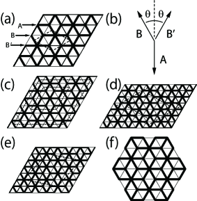
Figure 1: Distorted triangular lattice and finite-size clusters. Panel (a) illustrates sites A, B, and B^′ as well as the unit cell of the system. Panel (b) depicts the classical picture. The rhombuses in panel (c) illustrate finite-size clusters for $N_{\rm s}=9$ and 36 under the periodic boundary condition; rhombuses in panel (d) for $N_{\rm s}=12$ and 27; rhombus in panel (e) for $N_{\rm s}=21$. Panel (f) illustrates the $N_{\rm s}=37$ cluster under the open boundary condition.

Before observing our diagonalization results for the quantum case, let us consider the classical case composed of classical vectors with length $S$. A probable spin state is depicted in Fig. 1(b). For a given $r$, minimizing the energy determines the angle $\theta$ related to $M_{\rm spo}$. One obtains $M_{\rm spo}/M_{\rm sat}=1/3$ for $r\geq 2$ and $M_{\rm spo}/M_{\rm sat}=(r-1)/3$ for $1<r\leq 2$. The same spin state was discussed in ref. References.

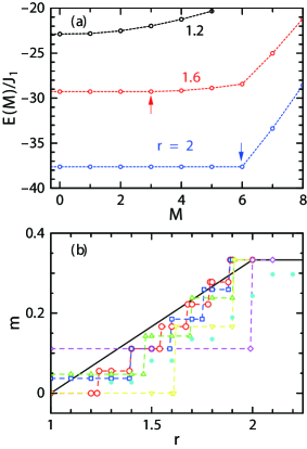
Figure 2: (Color) (a) $M$-dependence of the ground-state energy for $N_{\rm s}=36$. (b) $r$-dependence of the spontaneous magnetization for various system sizes. Violet diamonds, yellow reversed triangles, green triangles, blue squares, and red circles denote results for $N_{\rm s}=9$, 12, 21, 27, and 36 under the periodic boundary condition. Light blue closed circles denote results for $N_{\rm s}=37$ under the open boundary condition.

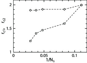
Figure 3: System-size dependence of the critical ratios for various system sizes. The squares and diamonds denote the results for $r_{\rm c1}$ and $r_{\rm c2}$, respectively.

Now, we present our results for the quantum case. First, our data for the lowest energy in each subspace of $M$ is shown in Fig. 2(a), which depicts the case for $N_{\rm s}=36$. This figure reveals whether a spontaneous magnetization occurs, and its magnitude if it occurs. For $r=1.2$, the energy for $M=0$ is lower than the energies for a larger $M$, which indicates that the ground state is nonmagnetic. For $r=1.6$, on the other hand, the energies for $M=0$ to 3 are numerically identical, which means that the system shows a spontaneous magnetization, and this magnetization is $M_{\rm spo}=3$. For $r=2$, the energies for $M=0$ to 6 are numerically identical, and the spontaneous magnetization $M_{\rm spo}=6$. Since the saturation is $M_{\rm sat}=18$ in the $N_{\rm s}=36$ system, $m=1/3$ suggests that the LM ferrimagnetic state is realized. Figure 2(a) strongly suggests that the present system shows gradual magnetization owing to the distortion $r>1$ between the nonmagnetic state and the LM ferrimagnetic state. These intermediate states may be interpreted as a collapse of ferrimagnetism occurring in the dice-lattice antiferromagnet. Note that we have so far investigated a collapse of ferrimagnetism occurring in the Lieb-lattice antiferromagnet by various distortions. The distorted kagome-lattice antiferromagnet shows a similar intermediate statecollapse_ferri2d ; Shimokawa_JPSJ , which will be compared to later. In other various distortions, such intermediate states were not detected so farshuriken_lett ; HN_kgm_dist ; HNakano_Cairo_lt ; Isoda_Cairo_full ; HN_TSakai_JJAP_RC .

Next, we examine the intermediate state in detail. Our results are depicted in Fig. 2(b). For $N_{\rm s}=9$, the nonmagnetic state of $M_{\rm spo}=1/2$ and the LM ferrimagnetic state of $M_{\rm spo}=3/2=(1/3)M_{\rm sat}$ are neighboring with each other without an intermediate $M_{\rm spo}$; however, this behavior comes from the smallness of $N_{\rm s}$. For a larger $N_{\rm s}$, there appear intermediate-$M_{\rm spo}$ states between the nonmagnetic state of $M_{\rm spo}=0$ or 1/2 and the LM ferrimagnetic state of $M_{\rm spo}=(1/3)M_{\rm sat}$. Note here that the states of all possible $M_{\rm spo}$ are realized between the smallest $M_{\rm spo}$ and $(1/3)M_{\rm sat}$ irrespective of $N_{\rm s}\geq 12$. Another marked behavior is that the range of the ratio $r$ of the intermediate $M_{\rm spo}$ gradually widens as $N_{\rm s}$ is increased. In order to clarify this behavior, we plot the $N_{\rm s}$-dependences of the critical ratios depicted in Fig. 3. Here, we define $r_{\rm c1}$ as the value of $r$ at which the ground state changes from $M_{\rm spo}=0$ or 1/2 to the next $M_{\rm spo}$, and $r_{\rm c2}$ as the value of $r$ at which the ground state changes to $M_{\rm spo}=(1/3)M_{\rm sat}$ from $M_{\rm spo}=(1/3)M_{\rm sat}-1$. Note that for $N_{\rm s}=9$, $r_{\rm c1}=r_{\rm c2}$ as mentioned above. One can easily observe that $r_{\rm c2}$ shows a very weak system size dependence. It is expected that an extrapolated value is $r_{\rm c2}\sim 1.9$. On the other hand, $r_{\rm c1}$ gradually decreases as $N_{\rm s}$ is increased. Although the dependence is not smooth, our numerical data suggest that an extrapolated value of $r_{\rm c1}$ is very close to $r=1$ corresponding to the case of the undistorted triangular lattice. It is difficult to determine $\lim_{N_{\rm s}\rightarrow\infty}r_{\rm c1}$ precisely from the present samples of finite sizes. To determine a reliable consequence concerning whether this limit is equal to 1 or different from 1, further investigations will be required. Note that even if this limit equals 1, such a consequence is consistent with the modern understanding of the triangular-lattice antiferromagnet, revealing the 120-degree spin structure in the ground state.

Let us compare the $r$-dependence of $M_{\rm spo}$ with the classical case, shown in Fig. 2(b). Our numerical data under the periodic boundary condition agree well with the solid line in the classical case illustrated in Fig. 1(b). This agreement seems to suggest that the intermediate-$M_{\rm spo}$ spin states in the quantum case can be understood based on the classical picture. In the following, let us examine whether this classical picture is valid in the quantum case from the viewpoint of the local magnetization $\langle S_{i}^{z}\rangle$. Here, the symbol $\langle{\cal O}\rangle$ represents the expectation value of the operator ${\cal O}$ with respect to the lowest-energy state within the subspace characterized by a magnetization $M_{\rm spo}$.

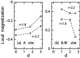
Figure 4: Site-dependence of the local magnetizations $\langle S_{i}^{z}\rangle$ for the system of $N_{\rm s}=37$. Distance $d$ is the distance between site $i$ and the center of the system with the open boundary, measured in units of the distance between two nearest-neighbor sites in the triangular lattice for $r=1$.

Figure 4 depicts the site-dependence of the local magnetizations for the system of $N_{\rm s}=37$ under the open boundary condition. Owing to this boundary condition, spin sites in each sublattice are not equivalent. The sites are divided into groups of equivalent sites characterized by the distance from the center of the cluster. Thus, we present our results in Fig. 4 as a function of the distance. We study the results for the case under the open boundary condition to compare a similar intermediate-$M_{\rm spo}$ state reported in the distorted kagome-lattice antiferromagnetcollapse_ferri2d ; Shimokawa_JPSJ , in which the local magnetizations show a nontrivial incommensurate modulation suggesting non-Lieb-Mattis ferrimagnetism. Note that the realizations of such incommensurate-modulation states were originally reported in several one-dimensional systems Ivanov_Richter ; Yoshikawa_Miya_JPSJ2005 ; Hida_JPSJ2007 ; Hida_JPCM2007 ; Hida_Takano_PRB2008 ; Montenegro_Coutinho_PRB2008 ; Hida_Takano_Suzuki_JPSJ2010 ; Shimokawa_Nakano_JPSJ2011 ; Furuya_Giamarchi_PRB2014 ; Hida_JPSJ2016 . Therefore, in this study, we focus on identifying the relationship between these incommensurate-modulation states and the intermediate states. We confirm that the intermediate-$M_{\rm spo}$ states appear in the case under the open boundary condition as depicted in the results in Fig. 2(b). Note that $m$ corresponding to the LM ferrimagnetism does not agree with 1/3 when $N_{\rm s}/3$ is not an integer. For $r=2.2$ in the present system, no significant behavior corresponding to incommensurate modulation is observed in our numerical data away from the boundary of the cluster when one excludes results on the open boundary, although a small boundary effect penetrates into the inside of the cluster. This is consistent with the fact that in this case, the LM ferrimagnetic state is realized. For $r=1.8$ in the present system, on the other hand, an intermediate-$M_{\rm spo}$ state appears. Even in such a state, our numerical data away from the boundary of the cluster do not show the behavior of incommensurate modulation. Therefore, our present results do not detect a direct evidence of the intermediate-$M_{\rm spo}$ state in the present system showing non-Lieb-Mattis ferrimagnetism. However, future studies under open boundary conditions should be carried out to clarify the relationship between these incommensurate-modulation states and the intermediate states in the present study.

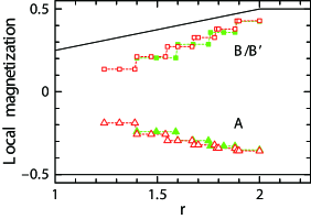
Figure 5: (Color) $r$-dependence of local magnetizations for $r\gtrsim r_{\rm c1}$. Solid lines represent the local magnetization from the classical picture. Squares denote the numerical results for the local magnetizations of B or B^′ sites; triangles denote those for A sites. Green closed symbols and red open symbols are for $N_{\rm s}=27$ and 36, respectively.

Next, we examine the $r$-dependence of the local magnetizations under the periodic boundary condition. Our numerical results for $N_{\rm s}=27$ and 36 in the region of $r\gtrsim r_{\rm c1}$ are depicted in Fig. 5. Note first that under this boundary condition, all spin sites in each sublattice are equivalent. Therefore, the numerical results of $\langle S_{i}^{z}\rangle$ at equivalent sites agree with each other within numerical errors. This is why how to present the numerical results of $\langle S_{i}^{z}\rangle$ is different between Figs. 4 and 5. A significant feature in Fig. 5 is that the results from the two sizes agree well with each other although our numerical results show step-like behaviors, which originate from a finite-size effect, as in Fig. 2(b). Owing to this serious finite-size effect, it is quite difficult to extrapolate finite-size $\langle S_{i}^{z}\rangle$ for a given fixed $r$ to the limit of $N_{\rm s}\rightarrow\infty$. Let us consider why we limit the region to be $r\gtrsim r_{\rm c1}$, in which our date are presented in Fig. 5. In this region, spontaneous magnetization occurs; therefore, the $z$-axis has a specific role, which means that the examination of the local magnetizations in Fig. 5 contributes considerably to our understanding of the magnetic structure of the intermediate states. If the spontaneously magnetized intermediate states show the same structure as the Y-shaped classical one, A-sublattice spins are supposed to be antiparallel to external field and B/B^′-sublattice spins are supposed to have components that are opposite to the A-sublattice spins. In Fig. 5, the lines from the Y-shaped classical picture are also illustrated. A marked behavior in the classical picture is that the down spin at an A-sublattice site maintains its local magnetization to be $-1/2$. On the other hand, in our numerical data, the local magnetization of an A-sublattice spin for the quantum systems gradually increase when $r$ is decreased from $r=2$ to $r=r_{\rm c1}$. Certainly, we have to be careful when the comparison is carried out between the classical system and the present behaviors of the finite-size quantum systems. This causes the mixing effect of magnetized states from a quantum nature just at $r=1$, which makes it difficult to detect a difference in the local magnetizations between the classical and quantum cases. However, for $r\gtrsim r_{\rm c1}$ away from $r=1$; such a difficulty does not occurs. An important difference of the quantum case from the classical one is that the local magnetization of an A-sublattice spin shows a significant dependence on $r$ in the quantum case. Generally speaking, there are two sources for changes of the local magnetization; one is a deviation of the spin amplitude and the other is the spin angle measured from the axis of the spontaneous magnetization. In the Y-shaped spin state within the classical picture, an A-sublattice spin is antiparallel to the axis of the spontaneous magnetization; namely, the spin angle vanishes. Recall here the spin amplitude of the 120-degree structure of the undistorted-triangular-lattice antiferromagnet from the spin-wave theoryJolicour_LGuillou , namely $\langle S_{z}\rangle=0.239$. In the present cases for $r\gtrsim r_{\rm c1}$, we are approaching the unfrustrated case of the dice lattice; therefore the possibility that the spin amplitude becomes smaller than $\langle S_{z}\rangle=0.239$ is quite low. Under this circumstance, we focus our attention on the numerical results of $N_{s}=36$ around $r=1.3$; we have $|\langle S_{i}^{z}\rangle|\sim 0.19$ for the A-sublattice spin. Such a small value of $|\langle S_{i}^{z}\rangle|$ cannot be explained only from the deviated spin amplitude without a change of the spin angle. Therefore, the spin state around $r=1.3$ of the quantum case is considered to be different from the Y-shaped spin state within the classical picture. The present analysis of the spin structure in the intermediate state is only the first step. For a deeper understanding of the spin structure, future investigations including a two-point correlation function and a chirality of the intermediate state are necessary.

Finally, we would like to comment on the experimental situation. Tanaka and Kakurai reported magnetic phase transitions of RbVBr₃, which shows a structure of a distorted triangular lattice, although the ratio of the interactions is consequently considered to be $r<1$Tanaka_Kakurai . Nishiwaki et al. studied RbFeBr₃, which also shows $r<1$Nishiwaki_jpsj2011 . A discovery of a new material with $1<r<2$ would give useful information concerning the intermediate state of ferrimagnetism from experiments.

In summary, we investigated the ground-state properties of the spin-$1/2$ Heisenberg antiferromagnet on the triangular lattice with a distortion by the numerical-diagonalization method. Under the conditions that the undistorted case is common with the triangular-lattice antiferromagnet without a magnetic field, and that the same up-up-down spin state is commonly realized both in the distorted case of the present model and in the $m$=1/3-plateau state of the triangular-lattice antiferromagnet under a magnetic field, we find that spontaneous magnetization grows along a new route to the $m$=1/3 up-up-down state due to the distortion of the lattice, which is different from the well-known route in the magnetization process of the triangular-lattice antiferromagnet. We are now examining this new state with intermediate spontaneous magnetization in more detail; the results will be published elsewhere.

We wish to thank Professors H. Sato, K. Yoshimura, N. Todoroki, and Miss A. Shimada for fruitful discussions. We wish to thank Dr. James Harries for his critical reading of our manuscript. This work was partly supported by JSPS KAKENHI Grant Numbers 16K05418, 16K05419, and 16H01080(JPhysics). Nonhybrid thread-parallel calculations in numerical diagonalizations were based on TITPACK version 2 coded by H. Nishimori. Some of the computations were performed using facilities of the Department of Simulation Science, National Institute for Fusion Science; Institute for Solid State Physics, The University of Tokyo; and Supercomputing Division, Information Technology Center, The University of Tokyo. This work was partly supported by the Strategic Programs for Innovative Research; the Ministry of Education, Culture, Sports, Science and Technology of Japan; and the Computational Materials Science Initiative, Japan.

References

- (1) P. W. Anderson, Mater. Res. Bull. 8, 153 (1973).
- (2) D. A. Huse and V. Elser, Phys. Rev. Lett. 60, 2531 (1988).
- (3) Th. Jolicour and J. C. Le Guillou, Phys. Rev. B 40, 2727 (1989).
- (4) R. R. P. Singh and D. A. Huse, Phys. Rev. Lett. 68, 1766 (1992).
- (5) B. Bernu, C. Lhuillier, and L. Pierre, Phys. Rev. Lett. 69, 2590 (1992).
- (6) B. Bernu, P. Lecheminant, C. Lhuillier, and L. Pierre, Phys. Rev. B 50, 10048 (1994).
- (7) P. W. Leung and K. J. Runge, Phys. Rev. B 47, 5861 (1993).
- (8) J. Richter, J. Schulenburg, and A. Honecker, Lecture Notes in Physics (Springer, Heidelberg, 2004) Vol. 645, p. 85.
- (9) T. Sakai and H. Nakano, Phys. Rev. B 83, 100405(R) (2011).
- (10) D. Yamamoto, G. Marmorini, and I. Danshita, Phys. Rev. Lett. 112, 127203 (2014)
- (11) Y. Shirata, H. Tanaka, T. Ono, A. Matsuo, K. Kindo, and H. Nakano: J. Phys. Soc. Jpn. 80 (2011) 093702.
- (12) Y. Shirata, H. Tanaka, A. Matsuo, K. Kindo, Phys. Rev. Lett. 108, 057205 (2012).
- (13) Z. Weihong, R. H. McKenzie, and R. R. P. Singh, Phys. Rev. B 59, 14367 (1999).
- (14) S. Yunoki and S. Sollera, Phys. Rev. B 74, 014408 (2006).
- (15) O. A. Starykh and L. Balents, Phys. Rev. Lett. 98, 077205 (2007).
- (16) D. Heidarian, S. Sollera, and F. Becca, Phys. Rev. B 80, 012404 (2009).
- (17) J. Reuther and R. Thomale, Phys. Rev. B 83, 024402 (2011).
- (18) A. Weichselbaum and S. R. White, Phys. Rev. B 84, 245130 (2011).
- (19) S. Ghamari, C. Kallin, S. S. Lee, and E. S. Sorensen, Phys. Rev. B 84, 174415 (2011).
- (20) K. Harada, Phys. Rev. B 86, 184421 (2012).
- (21) H. Nakano, S. Todo, and T. Sakai, J. Phys. Soc. Jpn. 82, 043715 (2013).
- (22) K. Watanabe, H. Kawamura, H. Nakano, and T. Sakai, J. Phys. Soc. Jpn. 83, 034714 (2014).
- (23) T. Shimokawa, K. Watanabe, and H. Kawamura, Phys. Rev. B 92, 134407 (2015).
- (24) A. Jagannathan and A. Szallas, Eur. Phys. J. B 86, 76 (2013).
- (25) E. Lieb and D. Mattis, J. Math. Phys. (N.Y.) 3, 749 (1962).
- (26) H. Nakano and A. Terai, J. Phys. Soc. Jpn. 78, 014003 (2009).
- (27) H. Nakano and T. Sakai, J. Phys. Soc. Jpn. 80, 053704 (2011).
- (28) H. Nakano and T. Sakai, J. Phys. Soc. Jpn. 83, 104710 (2014).
- (29) H. Nakano and T. Sakai, J. Phys. Soc. Jpn. 84, 063705 (2015).
- (30) H. Nakano, Y. Hasegawa, and T. Sakai, J. Phys. Soc. Jpn. 84, 114703 (2015).
- (31) Y. Nishiwaki, A. Osawa, K. Kakurai, K. Kaneko, M. Tokunaga, and T. Kato, J. Phys. Soc. Jpn. 80, 084711 (2011).
- (32) H. Nakano, T. Shimokawa, and T. Sakai, J. Phys. Soc. Jpn. 80, 033709 (2011).
- (33) T. Shimokawa and H. Nakano, J. Phys. Soc. Jpn. 81, 084710 (2012).
- (34) H. Nakano and T. Sakai, J. Phys. Soc. Jpn. 82, 083709 (2013).
- (35) H. Nakano, T. Sakai, and Y. Hasegawa, J. Phys. Soc. Jpn. 83, 084709 (2014).
- (36) H. Nakano, M. Isoda, and T. Sakai, J. Phys. Soc. Jpn. 83, 053702 (2014).
- (37) M. Isoda, H. Nakano, and T. Sakai, J. Phys. Soc. Jpn. 83, 084710 (2014).
- (38) H. Nakano and T. Sakai, Jpn. J. Appl. Phys. 54, 030305 (2015).
- (39) N. B. Ivanov and J. Richter: Phys. Rev. B 69, 214420 (2004).
- (40) S. Yoshikawa and S. Miyashita, Statistical Physics of Quantum Systems: novel orders and dynamics, J. Phys. Soc. Jpn. 74, (2005) Suppl., p. 71.
- (41) K. Hida, J. Phys. Soc. Jpn. 76, 024714 (2007).
- (42) K. Hida, J. Phys.: Condens. Matter 19, 145225 (2007).
- (43) K. Hida and K. Takano, Phys. Rev. B 78, 064407 (2008).
- (44) R. R. Montenegro-Filho and M. D. Coutinho-Filho, Phys. Rev. B 78, 014418 (2008).
- (45) K. Hida, K. Takano, and H. Suzuki, J. Phys. Soc. Jpn. 79, 114703 (2010).
- (46) T. Shimokawa and H. Nakano, J. Phys. Soc. Jpn. 80, 043703 (2011).
- (47) S. C. Furuya and T. Giamarchi, Phys. Rev. B 89, 205131 (2014).
- (48) K. Hida, J. Phys. Soc. Jpn. 85, 024705 (2016).
- (49) H. Tanaka and K. Kakurai, J. Phys. Soc. Jpn. 63, 3412 (1994).