Great Optically Luminous Dropout Research Using Subaru HSC (GOLDRUSH). I.
UV Luminosity Functions at $z\sim 4-7$
Derived with the Half-Million Dropouts
on the 100 deg² Sky

Abstract

We study the UV luminosity functions (LFs) at $z\sim 4$, $5$, $6,$ and $7$ based on the deep large-area optical images taken by the Hyper Suprime-Cam (HSC) Subaru strategic program (SSP). On the 100 deg² sky of the HSC SSP data available to date, we make enormous samples consisting of a total of 579,565 dropout candidates at $z\sim 4-7$ by the standard color selection technique, 358 out of which are spectroscopically confirmed by our follow-up spectroscopy and other studies. We obtain UV LFs at $z\sim 4-7$ that span a very wide UV luminosity range of $\sim 0.002$ – $100\,L_{\rm UV}^{\ast}$ ($-26<M_{\rm UV}<-14$ mag) by combining LFs from our program and the ultra-deep Hubble Space Telescope legacy surveys. We derive three parameters of the best-fit Schechter function, $\phi^{\ast}$, $M_{\rm UV}^{\ast}$, and $\alpha$, of the UV LFs in the magnitude range where the AGN contribution is negligible, and find that $\alpha$ and $\phi^{\ast}$ decrease from $z\sim 4$ to $7$ with no significant evolution of $M_{\rm UV}^{\ast}$. Because our HSC SSP data bridge the LFs of galaxies and AGNs with great statistical accuracy, we carefully investigate the bright end of the galaxy UV LFs that are estimated by the subtraction of the AGN contribution either aided with spectroscopy or the best-fit AGN UV LFs. We find that the bright end of the galaxy UV LFs cannot be explained by the Schechter function fits at $>2\sigma$ significance, and require either double power-law functions or modified Schechter functions that consider a magnification bias due to gravitational lensing.

1 Introduction

One of the important observables to study the formation and evolution of galaxies is the galaxy luminosity function (LF), which is the measure of the number of galaxies per unit volume as a function of luminosity. The form of the LF in the rest-frame UV is of significant interest, since it is closely related to ongoing star formation and contains key information about the physical processes that shape galaxies.

Great progress has been made in determining the faint end of the UV LFs (see the recent review of [Stark (2016)]). Analyses of sources in deep blank fields including the Hubble Ultra Deep field (HUDF) have resulted in identifying $z\sim 4-10$ galaxy candidates down to $\sim-17$ mag ([Ellis et al. (2013)]; [Schenker et al. (2013)]; [McLure et al. (2013)]; [Bouwens et al. (2015)]; [Finkelstein et al. (2015)]). Recently, it becomes possible to probe even fainter sources with the Hubble Frontier Fields (HFF) project, which takes advantage of the gravitational lens magnification effects of galaxy clusters ([Ishigaki et al. (2015)]; [Atek et al. (2015)]; [Kawamata et al. (2016)]; [Castellano et al. (2016)]; [McLeod et al. (2016)]; [Livermore et al. (2017)]; [Ishigaki et al. (2017)]). They have investigated the shape of the UV LF down to $\sim-14$ mag, at around which many cosmological hydrodynamic simulations of galaxy formation predict a flattening (e.g., [Muñoz & Loeb (2011)]; [Krumholz & Dekel (2012)]; [Kuhlen et al. (2013)]; [Jaacks et al. (2013)]; [Wise et al. (2014)]; [O’Shea et al. (2015)]; [Liu et al. (2016)]; [Gnedin (2016)]; [Ocvirk et al. (2016)]; [Finlator et al. (2017)]), although it has been pointed out that the analyses for the lensing fields would be significantly affected by systematic errors such as the one from the assumed size distribution of faint galaxies (Bouwens et al., 2017a) and the constructed magnification maps (Bouwens et al., 2017b).

Together with studying the faint end of the UV LFs, it is important to investigate their bright-end shapes. Previous studies have shown that the UV LF of low-$z$ galaxies has an exponential cutoff (e.g., Loveday et al. (2012); Kelvin et al. (2014)), which is thought to be caused by several different mechanisms such as heating from an active galactic nucleus (AGN; Binney (2004); Scannapieco & Oh (2004); Granato et al. (2004); Croton et al. (2006); Bower et al. (2006)), inefficiency of gas cooling in high-mass dark matter haloes (e.g., Binney (1977); Rees & Ostriker (1977); Silk (1977); Benson et al. (2003)), and dust attenuation, which becomes substantial for the most luminous galaxies (e.g., Wang & Heckman (1996); Adelberger & Steidel (2000); Martin et al. (2005)). However, at very high redshifts where typical dark matter halo masses are small, these processes may be ineffective yet (e.g., Bouwens et al. (2008)). Interestingly, recent studies by Bowler et al. (2015) and Bowler et al. (2017) using a $1.7$ deg² imaging survey have claimed an overabundance of galaxies at the bright end of the $z\geq 6$ LF over the best-fit Schechter function. It may indicate different astrophysical conditions in high-$z$ and low-$z$ galaxies. Another possible explanation for the overabundance at the bright end is contribution of light from AGNs. At a lower redshift of $z\sim 3$, around the peak of the quasar number density, there is evidence that the UV LF at the absolute UV magnitude $M_{\rm UV}\lesssim-24$ mag has a significant contribution from faint quasars (Bian et al., 2013). Gravitational lensing magnification bias also needs to be considered (Wyithe et al., 2011; Takahashi et al., 2011; Mason et al., 2015; Barone-Nugent et al., 2015). It is also possible that merger systems are blended at ground-based resolution and appear as bright extended objects (Bowler et al., 2017). Due to the small number densities of these luminous galaxies, previous studies lack information on the most luminous $z\gtrsim 4$ galaxies with $M_{\rm UV}\lesssim-23$ mag (e.g., Ouchi et al. (2004); Shimasaku et al. (2005); Sawicki & Thompson (2006); Yoshida et al. (2006); Iwata et al. (2007); McLure et al. (2009); Ouchi et al. (2009); Castellano et al. (2010); van der Burg et al. (2010); Willott et al. (2013); Bowler et al. (2015); Bowler et al. (2017); Stefanon et al. (2017)). To study a possible deviation from the commonly used Schechter functional form, it is necessary to construct a sample of rare luminous high-$z$ galaxies down to very low space densities based on wider multi-wavelength deep imaging surveys. In addition, spectroscopic redshifts for a subsample are vital to estimate the contaminant fraction for LF calculation.

In this study, we present results from our systematic search for very luminous galaxies at $z\sim 4-7$ based on wide and deep optical Hyper Suprime-Cam (HSC; Miyazaki et al. (2012); see also Miyazaki et al. (2017); Komiyama et al. (2017); Furusawa et al. (2017); Kawanomoto et al. (2017)) images obtained by the Subaru Strategic Program (HSC SSP; Aihara et al. (2017b)). With a large field of view of about $1.8$ deg² and excellent sensitivity, HSC is one of the best ground-based instruments for searching for intrinsically luminous but apparently faint rare sources such as luminous high-$z$ galaxies. The HSC SSP survey was awarded 300 nights of Subaru observing time over 5 years from 2014. The survey consists of three layers: Wide (W), Deep (D), and UltraDeep (UD). The W layer will cover $1400$ deg² with five broadband filters of $g$, $r$, $i$, $z$, and $y$ down to $5\sigma$ limits of about $26$ mag ($24-25$ mag) in $gri$ ($zy$). The D (UD) layers will cover $27$ ($3.5$) deg² with the five broadband filters down to $5\sigma$ limits of about $27$ ($28$) mag in $gri$ and $25-26$ ($26-27$) mag in $zy$. The D (UD) layers will also be observed with three narrowband filters of NB387 (NB101), NB816, and NB921. Public versions of the reduced HSC SSP images and source catalogs are available to the community on the HSC SSP website. This wide-field deep survey will enable us to cover an unprecedentedly large cosmic volume at $z\gtrsim 4$ and to identify a large number of very rare bright sources that reside at the bright end of the UV LF, which has been poorly explored by previous high-$z$ galaxy studies. The present paper is one in a series of papers from twin continuing programs devoted to scientific results on high-$z$ galaxies based on the HSC SSP survey data products. One program is Great Optically Luminous Dropout Research Using Subaru HSC (GOLDRUSH). This program provides precise determinations of the the very bright end of the galaxy UV LFs at $z\sim 4-7$, which are presented in this paper, robust clustering measurements of luminous galaxy candidates at $z\sim 4-6$ (Harikane et al., 2017), and construction of a sizable sample of $z\sim 4$ galaxy protocluster candidates (Toshikawa et al., 2017). The other program is Systematic Identification of LAEs for Visible Exploration and Reionization Research Using Subaru HSC (SILVERRUSH; Ouchi et al. (2017); Shibuya et al. (2017a); Shibuya et al. (2017b); Konno et al. (2017); R. Higuchi et al. in preparation). Data products from these programs such as catalogs of dropouts and LAEs will be provided on our project webpage at http://cos.icrr.u-tokyo.ac.jp/rush.html.

This paper is organized as follows. In the next section, we describe our HSC SSP data and spectroscopic follow-up observations. The sample selection and analyses for measuring UV LF are described in Section 3. We show the results of our UV LF measurements and discuss the shapes of the UV LFs in Section 4. A summary is presented in Section 5. Throughout this paper, we use magnitudes in the AB system (Oke & Gunn, 1983) and assume a flat universe with $\Omega_{\rm m}=0.3$, $\Omega_{\Lambda}=0.7$, and $H_{0}=70$ km s^-1 Mpc^-1.

ccccccccc HSC SSP data used in this study. (1) Field name. (2) Right ascension. (3) Declination. (4) Effective area in deg². (5)–(9) $5\sigma$ limiting magnitude measured with $1\farcs 5$ diameter circular apertures in $g$, $r$, $i$, $z$, and $y$. Field R.A. Decl. Area $g$ $r$ $i$ $z$ $y$
(J2000) (J2000) (deg²) (ABmag) (ABmag) (ABmag) (ABmag) (ABmag)
(1) (2) (3) (4) (5) (6) (7) (8) (9)
UltraDeep (UD)
UD-SXDS 02:18:00.00 $-$05:00:00.00 $1.1$ $27.15$ $26.68$ $26.53$ $25.96$ $25.15$
UD-COSMOS 10:00:28.60 02:12:21.00 $1.3$ $27.13$ $26.84$ $26.46$ $26.10$ $25.28$
Deep (D)
D-XMM-LSS 02:16:51.57 $-$03:43:08.43 $2.4$ $26.73$ $26.30$ $25.88$ $25.42$ $24.40$
D-COSMOS 10:00:59.50 02:13:53.06 $6.5$ $26.56$ $26.19$ $26.04$ $25.58$ $24.76$
D-ELAIS-N1 16:10:00.00 54:17:51.07 $3.3$ $26.77$ $26.13$ $25.87$ $25.16$ $24.25$
D-DEEP2-3 23:30:22.22 $-$00:44:37.69 $5.5$ $26.69$ $26.25$ $25.96$ $25.29$ $24.56$
Wide (W)
W-XMM 02:16:51.57 $-$03:43:08.43 $28.5$ $26.43$ $25.93$ $25.71$ $25.00$ $24.25$
W-GAMA09H 09:05:11.11 00:44:37.69 $12.4$ $26.35$ $25.88$ $25.65$ $25.07$ $24.45$
W-WIDE12H 11:57:02.22 00:44:37.69 $15.2$ $26.38$ $25.95$ $25.82$ $25.15$ $24.23$
W-GAMA15H 14:31:06.67 $-$00:44:37.69 $16.6$ $26.39$ $25.96$ $25.81$ $25.11$ $24.31$
W-HECTOMAP 16:08:08.14 43:53:03.47 $4.8$ $26.47$ $26.04$ $25.82$ $25.09$ $24.07$
W-VVDS 22:37:02.22 00:44:37.69 $5.1$ $26.31$ $25.87$ $25.74$ $24.98$ $24.23$
Total — — $102.7$ — — — — —

llcl The selection criteria for our source catalog construction. Parameter Value Band Comment
detect_is_primary True — Object is a primary one with no deblended children.
flags_pixel_edge False $grizy$ Locate within images
flags_pixel_interpolated_center False $grizy$ None of the central $3\times 3$ pixels of an object is interpolated.
flags_pixel_saturated_center False $grizy$ None of the central $3\times 3$ pixels of an object is saturated.
flags_pixel_cr_center False $grizy$ None of the central $3\times 3$ pixels of an object is masked as cosmic ray.
flags_pixel_bad False $grizy$ None of the pixels in the footprint of an object is labelled as bad.
flags_pixel_bright_object_any False $grizy$ None of the pixels in the footprint of an object is close to bright sources.
centroid_sdss_flags False $ri$ for $g$-drop Object centroid measurement has no problem.
False $iz$ for $r$-drop
False $zy$ for $i$-drop
False $y$ for $z$-drop
cmodel_flux_flags False $gri$ for $g$-drop Cmodel flux measurement has no problem.
False $riz$ for $r$-drop
False $izy$ for $i$-drop
False $zy$ for $z$-drop
merge_peak True $ri$ for $g$-drop Detected in $r$ and $i$
False/True $g$/$iz$ for $r$-drop Undetected in $g$ and detected in $r$ and $i$
False/True $gr$/$zy$ for $i$-drop Undetected in $g$ and $r$, and detected in $z$ and $y$
False/True $gri$/$y$ for $z$-drop Undetected in $g$, $r$ and $i$, and detected in $y$
blendedness_abs_flux $<0.2$ $ri$ for $g$-drop The target photometry is not significantly affected by neighbors.
$<0.2$ $iz$ for $r$-drop
$<0.2$ $zy$ for $i$-drop
$<0.2$ $y$ for $z$-drop

2 Data

2.1 Imaging Data

In this study, we use early data products of the HSC SSP that are obtained in 2014–2016 (Aihara et al., 2017a). Specifically, we use the internal data release of S16A, where additional data taken in 2016 January – April have been merged with the version of Public Data Release 1. The HSC images were reduced with version 4.0.2 of the HSC pipeline, hscPipe (Bosch et al., 2017), which uses codes from the Large Synoptic Survey Telescope (LSST) software pipeline (Ivezic et al., 2008; Axelrod et al., 2010; Jurić et al., 2015). The HSC pipeline performs CCD-by-CCD reduction, calibration for astrometry, and photometric zero point determination. The pipeline then conducts mosaic-stacking that combines reduced CCD images into a large stacked image, and creates source catalogs by detecting and measuring sources on the stacked images. The HSC astrometry and photometry are calibrated with the Pan-STARRS $3\pi$ catalog (Tonry et al., 2012; Schlafly et al., 2012; Magnier et al., 2013). Full details of the HSC observations, data reduction, and object detection and photometric catalog creation are provided in Aihara et al. (2017a). In this study, we estimate total magnitudes and colors of sources by using the cmodel magnitude, which is a weighted combination of exponential and de Vaucouleurs fits to the light profile of each object (Abazajian et al. (2004); Bosch et al. (2017)). The source colors are measured through forced photometry. We correct all the magnitudes for Galactic extinction by using the dust map of Schlegel et al. (1998).

The current HSC SSP survey data cover $6$ distinct areas on the sky in the W layer, $4$ areas in the D layer, and $2$ areas in the UD layer. To obtain uniform data sets, we mask regions which are affected by bright source halos (Coupon et al., 2017). We also mask regions where exposure times are relatively short by using the hscPipe parameter countinputs $N_{\rm c}$, which denotes the number of exposures at a source position for a given filter. For the W-layer data, regions where $N_{\rm c}\geq(3,\,3,\,5,\,5,\,5)$ for $(g,\,r,\,i,\,z,\,y)$ are used. For the D-layer data, regions where $N_{\rm c}\geq(3,\,3,\,5,\,5,\,5)$ for $(g,\,r,\,i,\,z,\,y)$ are used. For the UD-COSMOS data, regions where $N_{\rm c}\geq(17,\,16,\,27,\,47,\,62)$ for $(g,\,r,\,i,\,z,\,y)$ are used. For the UD-SXDS data, regions where $N_{\rm c}\geq(13,\,13,\,27,\,42,\,38)$ for $(g,\,r,\,i,\,z,\,y)$ are used. After the masks are applied, the total effective area is about $100$ deg². Thanks to the large volumes that we probe, the influence of cosmic variance on the shape of the estimated LF is expected to be small (Trenti & Stiavelli, 2008). Table 1 summarizes the effective areas and the $5\sigma$ limiting magnitudes of our data.

First, we select isolated or cleanly deblended sources from the detected source catalog available on the database (Takata et al., 2017) that is provided by the HSC SSP survey team. We then require that none of the pixels in their footprint are interpolated, none of the central $3\times 3$ pixels are saturated, none of the central $3\times 3$ pixels are affected by cosmic rays, and there are no bad pixels in their footprint. We also require that there are no problems in measuring cmodel fluxes in $gri$ images for $g$-dropouts, in $riz$ images for $r$-dropouts, in $izy$ images for $i$-dropouts, and in $zy$ images for $z$-dropouts. In addition, we remove sources if there are any problems in measuring their centroid positions in $ri$ images for $g$-dropouts, in $iz$ images for $r$-dropouts, in $zy$ images for $i$-dropouts, and in $y$ images for $z$-dropouts. The selection criteria for our source catalog construction are listed in Table 1.

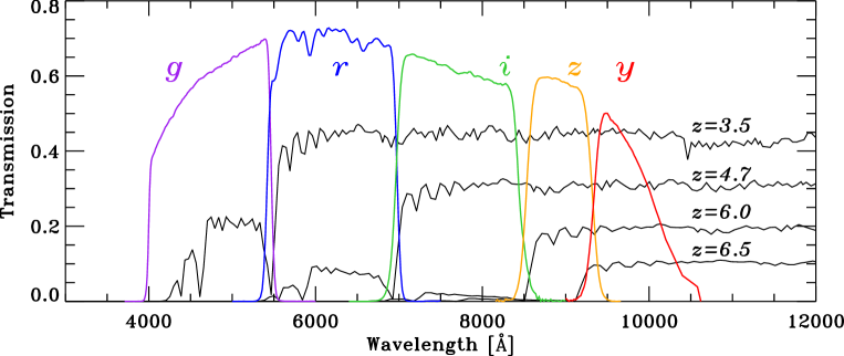
Figure 1: Transmissions of the five HSC broadband filters used in this study (purple: $g$, blue: $r$, green: $i$, orange: $z$, and red: $y$) together with four spectra of star-forming galaxies at $z=3.5$, $4.7$, $6.0$, and $6.5$ from the Bruzual & Charlot (2003) library (black lines).

2.2 Spectroscopic Data

We carried out spectroscopic follow-up observations for sources in our catalogs with the Faint Object Camera and Spectrograph (FOCAS; Kashikawa et al. (2002)) on the Subaru Telescope on 2015 September 7 (S15B-188S, PI: Y. Ono), December 2, 4 (S15B-059, PI: S. Yuma), and 12 (S16A-211S, PI: Y. Ono), and with the Low Dispersion Survey Spectrograph 3 (LDSS3) on the Magellan II Clay telescope in 2015 November (PI: M. Rauch). Our sources were filler targets in the FOCAS observations of S15B-059 and the LDSS observations. In the FOCAS observations, we used the $300$ line mm^-1 grism and the VPH900 grism with the SO58 order-cut filter. The spectroscopic observations were made in the long slit mode or multi-object slit mode. Slit widths were 0$\farcs$8. The integration times were 2,000–6,000 sec. Flux calibration was carried out with spectra of the spectroscopic standard stars G191B2B, Feige 34, and GD153. In the LDSS3 observations, the VPH RED grism and the OG590 filter were used. The spectroscopic observations were made in the long slit mode. Slit widths were $1\farcs 0$. The integration times were 3,600–5,400 sec. Flux calibration was carried out with spectra of the spectroscopic standard star LTT 9239. Note that we have also been awarded observing time with the Gemini Multi-Object Spectrographs (GMOS; Hook et al. (2004)) on the Gemini South telescope (PI: M. Sawicki), but at the time of writing this paper, no useful data had yet been obtained from this program.

In addition to the observations described above, we include results of our observations with the Inamori Magellan Areal Camera and Spectrograph (IMACS; Dressler et al. (2011)) on the Magellan I Baade telescope in 2007 – 2011 (PI: M. Ouchi). The IMACS observations were carried out on 2007 November 11–14, 2008 November 29–30, December 1–2, December 18–20, 2009 October 11–13, 2010 February 8–9, July 9–10, and 2011 January 3–4. In these observations, main targets were high-$z$ Ly$\alpha$ emitter (LAE) candidates found in the deep Subaru Suprime-Cam narrowband images obtained in the SXDS (Ouchi et al., 2008, 2010) and COSMOS fields (Murayama et al., 2007; Shioya et al., 2009), and high-$z$ dropout galaxy candidates selected from the deep broadband images in these two fields (Furusawa et al., 2008; Capak et al., 2007) were also observed as mask fillers. The data are reduced with the Carnegie Observatories System for MultiObject Spectroscopy (cosmos) pipeline. Details of the IMACS observations and data reduction will be presented elsewhere.

Number of Sources in our $z\sim 4$, $z\sim 5$, $z\sim 6$, and $z\sim 7$ Galaxy Candidate Samples. Field $z\sim 4$ $z\sim 5$ $z\sim 6$ $z\sim 7$ # # # # UltraDeep (UD) UD-SXDS $9916$ $1209$ $36$ —^† UD-COSMOS $10644$ $1990$ $50$ —^† Deep (D) D-XMM-LSS $6730$ $711$ $6$ $0$ D-COSMOS $45767$ $6282$ $64$ $4$ D-ELAIS-N1 $19631$ $612$ $15$ $1$ D-DEEP2-3 $35963$ $1498$ $47$ $5$ Wide (W) W-XMM $113582$ $6371$ $81$ $7$ W-GAMA09H $44670$ $5989$ $98$ $16$ W-WIDE12H $94544$ $5243$ $36$ $8$ W-GAMA15H $104224$ $6457$ $73$ $14$ W-HECTOMAP $30663$ $1082$ $11$ $7$ W-VVDS $23677$ $1500$ $20$ $11$ Total $540011$ $38944$ $537$ 73 ^† Our $z\sim 7$ dropout search focuses on the W and D layers. See Section 3.1 for details.

ccccccccc Spectroscopically identified galaxies and AGNs in our dropout samples. (1) Object ID. (2) Right ascension. (3) Declination. (4) Spectroscopic redshift. (5) Apparent magnitude. (6) UV absolute magnitude. (7) The dropout sample in which the source is selected: 1 = $g$-dropout, 2 = $r$-dropout, 3 = $i$-dropout, and 4 = $z$-dropout. (8) Galaxy/AGN flag (1 = galaxy; 2 = AGN). (9) Reference of spectroscopic redshift. S08 = Saito et al. (2008), O08 = Ouchi et al. (2008), W10 = Willott et al. (2010a), C12 = Curtis-Lake et al. (2012), Mas12 = Masters et al. (2012), M12 = Mallery et al. (2012), W13 = Willott et al. (2013), L13 = Le Fèvre et al. (2013), K15 = Kashikawa et al. (2015), Kr15 = Kriek et al. (2015), W16 = Wang et al. (2016), T16 = Toshikawa et al. (2016), Mo16 = Momcheva et al. (2016), M16 = Matsuoka et al. (2016), P17 = Pâris et al. (2017), T17 = Tasca et al. (2017), Y17 = Yang et al. (2017), Mas17 = Masters et al. (2017), M17 = Matsuoka et al. (2017), S17 = Shibuya et al. (2017b), and H17 = R. Higuchi et al. in preparation. ID R.A. Decl. $z_{\rm spec}$ $m$ $M_{\rm UV}$ Sample Flag Reference
(J2000) (J2000) (mag) (mag)
(1) (2) (3) (4) (5) (6) (7) (8) (9)
Galaxies
HSC J015949–035945 01:59:49.36 $-$03:59:45.24 $5.770$ $24.0$ $-22.7$ 3 1 M17
HSC J021033–052304 02:10:33.82 $-$05:23:04.28 $5.890$ $23.7$ $-23.0$ 3 1 M16
HSC J021041–055917 02:10:41.28 $-$05:59:17.87 $5.820$ $24.3$ $-22.4$ 3 1 M16
HSC J021545–055529 02:15:45.20 $-$05:55:29.03 $5.740$ $23.9$ $-22.7$ 3 1 M16
HSC J021551–050938 02:15:51.21 $-$05:09:38.49 $4.848$ $24.5$ $-21.8$ 2 1 This Study
HSC J021624–045516 02:16:24.70 $-$04:55:16.55 $5.706$ $25.7$ $-20.9$ 2 1 H17
HSC J021640–050129 02:16:40.67 $-$05:01:29.43 $3.699$ $24.4$ $-21.5$ 1 1 O08
HSC J021654–050216 02:16:54.14 $-$05:02:16.50 $4.284$ $25.7$ $-20.5$ 1 1 This Study
HSC J021658–053419 02:16:58.03 $-$05:34:19.17 $3.790$ $25.4$ $-20.5$ 1 1 S08
HSC J021704–045215 02:17:04.17 $-$04:52:15.69 $4.826$ $24.9$ $-21.4$ 2 1 This Study
HSC J021708–043301 02:17:08.19 $-$04:33:01.45 $5.005$ $25.2$ $-21.2$ 2 1 This Study
HSC J021711–050806 02:17:11.20 $-$05:08:06.44 $4.084$ $22.8$ $-23.3$ 1 1 Mo16
HSC J021712–051041 02:17:12.45 $-$05:10:41.44 $4.371$ $24.9$ $-21.3$ 1 1 Mo16
HSC J021714–044510 02:17:14.01 $-$04:45:10.77 $3.988$ $25.6$ $-20.5$ 1 1 This Study
HSC J021714–052516 02:17:14.71 $-$05:25:16.07 $3.729$ $25.6$ $-20.3$ 1 1 O08
HSC J021715–044418 02:17:15.29 $-$04:44:18.21 $3.980$ $25.2$ $-20.8$ 1 1 This Study
HSC J021715–044751 02:17:15.98 $-$04:47:51.54 $3.700$ $24.6$ $-21.3$ 1 1 This Study
HSC J021716–044336 02:17:16.54 $-$04:43:36.90 $4.808$ $25.0$ $-21.3$ 2 1 This Study
HSC J021718–044945 02:17:18.33 $-$04:49:45.29 $4.356$ $25.4$ $-20.8$ 1 1 This Study
HSC J021719–044853 02:17:19.13 $-$04:48:53.46 $4.239$ $25.8$ $-20.3$ 1 1 This Study
HSC J021721–050046 02:17:21.96 $-$05:00:46.83 $3.666$ $24.8$ $-21.0$ 1 1 This Study
HSC J021722–053059 02:17:22.01 $-$05:30:59.58 $3.798$ $24.6$ $-21.3$ 1 1 This Study
HSC J021723–044315 02:17:23.74 $-$04:43:15.81 $4.034$ $24.5$ $-21.6$ 1 1 This Study
HSC J021726–051839 02:17:26.07 $-$05:18:39.38 $4.077$ $24.5$ $-21.5$ 1 1 This Study
HSC J021727–044202 02:17:27.49 $-$04:42:02.31 $3.971$ $24.0$ $-22.0$ 1 1 This Study
HSC J021727–044413 02:17:27.70 $-$04:44:13.81 $3.683$ $25.7$ $-20.2$ 1 1 O08
HSC J021734–050514 02:17:34.38 $-$05:05:14.53 $3.986$ $23.3$ $-22.7$ 1 1 This Study
HSC J021734–044558 02:17:34.57 $-$04:45:58.95 $5.702$ $25.4$ $-21.2$ 2 1 H17
HSC J021735–051032 02:17:35.33 $-$05:10:32.42 $6.120$ $24.8$ $-21.9$ 3 1 C12
HSC J021736–043334 02:17:36.06 $-$04:33:34.87 $4.293$ $25.9$ $-20.3$ 1 1 This Study
HSC J021736–044549 02:17:36.39 $-$04:45:49.10 $4.019$ $24.9$ $-21.1$ 1 1 This Study
HSC J021737–044650 02:17:37.85 $-$04:46:50.35 $3.899$ $24.9$ $-21.0$ 1 1 This Study
HSC J021738–052057 02:17:38.93 $-$05:20:57.91 $4.110$ $26.2$ $-19.9$ 1 1 S08
HSC J021739–044832 02:17:39.78 $-$04:48:32.82 $3.889$ $25.3$ $-20.7$ 1 1 This Study
HSC J021739–053253 02:17:39.89 $-$05:32:53.68 $4.487$ $24.5$ $-21.7$ 2 1 This Study
HSC J021740–045103 02:17:40.34 $-$04:51:03.55 $4.545$ $25.4$ $-20.8$ 1 1 This Study
HSC J021742–043608 02:17:42.73 $-$04:36:08.80 $4.397$ $25.6$ $-20.6$ 1 1 This Study
HSC J021744–050642 02:17:44.56 $-$05:06:42.41 $4.549$ $24.6$ $-21.7$ 1 1 This Study
HSC J021744–044401 02:17:44.63 $-$04:44:01.64 $4.377$ $26.0$ $-20.2$ 1 1 This Study
HSC J021745–052735 02:17:45.37 $-$05:27:35.55 $3.648$ $24.5$ $-21.3$ 1 1 O08
HSC J021746–051553 02:17:46.01 $-$05:15:53.54 $4.037$ $24.8$ $-21.2$ 1 1 This Study
HSC J021746–045045 02:17:46.14 $-$04:50:45.67 $4.039$ $25.1$ $-20.9$ 1 1 This Study
HSC J021747–045229 02:17:47.71 $-$04:52:29.85 $3.648$ $23.8$ $-22.0$ 1 1 O08
HSC J021748–044935 02:17:48.97 $-$04:49:35.64 $4.221$ $26.3$ $-19.8$ 1 1 This Study
HSC J021749–043753 02:17:49.54 $-$04:37:53.04 $4.212$ $25.4$ $-20.8$ 1 1 This Study
HSC J021750–043230 02:17:50.86 $-$04:32:30.52 $4.095$ $26.1$ $-20.0$ 1 1 This Study
HSC J021751–052637 02:17:51.00 $-$05:26:37.54 $4.920$ $24.2$ $-22.2$ 2 1 This Study
HSC J021751–045627 02:17:51.01 $-$04:56:27.44 $3.701$ $25.7$ $-20.2$ 1 1 This Study
HSC J021752–053120 02:17:52.06 $-$05:31:20.93 $4.109$ $24.9$ $-21.2$ 1 1 This Study
HSC J021752–050700 02:17:52.78 $-$05:07:00.15 $3.700$ $25.9$ $-19.9$ 1 1 This Study
HSC J021754–050913 02:17:54.87 $-$05:09:13.80 $3.704$ $26.2$ $-19.7$ 1 1 This Study
HSC J021755–043203 02:17:55.30 $-$04:32:03.70 $4.626$ $24.5$ $-21.7$ 1 1 This Study
HSC J021756–053352 02:17:56.82 $-$05:33:52.97 $3.986$ $25.1$ $-21.0$ 1 1 This Study
HSC J021758–052135 02:17:58.22 $-$05:21:35.54 $4.646$ $25.7$ $-20.6$ 1 1 This Study
HSC J021758–043417 02:17:58.42 $-$04:34:17.68 $4.082$ $24.6$ $-21.5$ 1 1 This Study
HSC J021759–052507 02:17:59.47 $-$05:25:07.57 $3.820$ $26.1$ $-19.9$ 1 1 S08
HSC J021800–052410 02:18:00.11 $-$05:24:10.46 $4.470$ $25.7$ $-20.5$ 1 1 S08
HSC J021803–022029 02:18:03.42 $-$02:20:29.73 $5.900$ $24.0$ $-22.7$ 3 1 M17
HSC J021807–052048 02:18:07.74 $-$05:20:48.03 $3.638$ $25.0$ $-20.8$ 1 1 O08
HSC J021808–044845 02:18:08.12 $-$04:48:45.54 $4.852$ $25.1$ $-21.3$ 2 1 This Study
HSC J021813–051505 02:18:13.31 $-$05:15:05.25 $4.270$ $25.5$ $-20.7$ 1 1 S08
HSC J021813–051841 02:18:13.53 $-$05:18:41.03 $3.572$ $23.9$ $-21.9$ 1 1 This Study
HSC J021813–043057 02:18:13.56 $-$04:30:57.07 $3.668$ $25.6$ $-20.3$ 1 1 O08
HSC J021813–051840 02:18:13.79 $-$05:18:40.91 $5.013$ $24.2$ $-22.2$ 2 1 This Study
HSC J021814–043904 02:18:14.15 $-$04:39:04.39 $4.469$ $24.9$ $-21.3$ 1 1 This Study
HSC J021817–051027 02:18:17.08 $-$05:10:27.32 $3.702$ $25.6$ $-20.3$ 1 1 This Study
HSC J021823–051121 02:18:23.76 $-$05:11:21.32 $3.681$ $25.9$ $-20.0$ 1 1 This Study
HSC J021825–044429 02:18:25.06 $-$04:44:29.20 $4.023$ $25.2$ $-20.8$ 1 1 This Study
HSC J021826–051003 02:18:26.22 $-$05:10:03.47 $3.699$ $25.0$ $-20.9$ 1 1 O08
HSC J021827–051947 02:18:27.71 $-$05:19:47.18 $3.677$ $25.8$ $-20.1$ 1 1 O08
HSC J021828–042956 02:18:28.94 $-$04:29:56.05 $4.344$ $26.0$ $-20.1$ 1 1 This Study
HSC J021830–052808 02:18:30.79 $-$05:28:08.55 $3.579$ $23.8$ $-22.1$ 1 1 This Study
HSC J021832–043827 02:18:32.62 $-$04:38:27.68 $4.212$ $25.9$ $-20.2$ 1 1 This Study
HSC J021835–053550 02:18:35.18 $-$05:35:50.45 $3.671$ $25.1$ $-20.7$ 1 1 O08
HSC J021835–042321 02:18:35.94 $-$04:23:21.63 $5.755$ $24.9$ $-21.7$ 2 1 S17
HSC J021836–043906 02:18:36.29 $-$04:39:06.85 $3.797$ $25.3$ $-20.6$ 1 1 This Study
HSC J021837–044603 02:18:37.70 $-$04:46:03.47 $4.635$ $24.7$ $-21.5$ 1 1 This Study
HSC J021838–052023 02:18:38.50 $-$05:20:23.05 $3.678$ $25.1$ $-20.7$ 1 1 This Study
HSC J021838–050943 02:18:38.90 $-$05:09:43.94 $6.190$ $25.0$ $-21.8$ 3 1 C12
HSC J021842–052340 02:18:42.06 $-$05:23:40.24 $4.722$ $23.8$ $-22.5$ 2 1 This Study
HSC J021845–052718 02:18:45.54 $-$05:27:18.72 $3.676$ $25.3$ $-20.6$ 1 1 This Study
HSC J021845–044139 02:18:45.56 $-$04:41:39.19 $4.016$ $25.1$ $-20.9$ 1 1 This Study
HSC J021848–043755 02:18:48.15 $-$04:37:55.06 $3.659$ $24.9$ $-20.9$ 1 1 This Study
HSC J021848–050224 02:18:48.77 $-$05:02:24.22 $4.599$ $26.1$ $-20.1$ 1 1 This Study
HSC J021851–052228 02:18:51.24 $-$05:22:28.39 $3.671$ $24.6$ $-21.3$ 1 1 This Study
HSC J021851–043022 02:18:51.31 $-$04:30:22.86 $4.353$ $25.6$ $-20.6$ 1 1 This Study
HSC J021852–043832 02:18:52.25 $-$04:38:32.69 $3.769$ $26.1$ $-19.9$ 1 1 This Study
HSC J021852–053008 02:18:52.93 $-$05:30:08.02 $3.819$ $23.7$ $-22.3$ 1 1 This Study
HSC J021853–044628 02:18:53.62 $-$04:46:28.14 $3.894$ $25.6$ $-20.3$ 1 1 This Study
HSC J021856–044556 02:18:56.66 $-$04:45:56.37 $4.125$ $24.8$ $-21.3$ 1 1 This Study
HSC J021911–045646 02:19:11.65 $-$04:56:46.72 $5.009$ $24.8$ $-21.6$ 2 1 This Study
HSC J021915–045511 02:19:15.37 $-$04:55:11.87 $3.672$ $25.4$ $-20.5$ 1 1 O08
HSC J021917–050739 02:19:17.32 $-$05:07:39.26 $3.693$ $25.0$ $-20.9$ 1 1 O08
HSC J021921–045712 02:19:21.19 $-$04:57:12.51 $4.790$ $24.9$ $-21.5$ 2 1 This Study
HSC J021930–050915 02:19:30.57 $-$05:09:15.86 $4.580$ $22.8$ $-23.5$ 2 1 This Study
HSC J021938–045405 02:19:38.21 $-$04:54:05.18 $4.914$ $25.1$ $-21.3$ 2 1 This Study
HSC J021942–045525 02:19:42.18 $-$04:55:25.51 $4.226$ $25.3$ $-20.8$ 1 1 This Study
HSC J021944–045055 02:19:44.67 $-$04:50:55.56 $3.669$ $25.5$ $-20.4$ 1 1 O08
HSC J021948–045606 02:19:48.60 $-$04:56:06.79 $5.074$ $25.2$ $-21.2$ 2 1 This Study
HSC J021950–050845 02:19:50.63 $-$05:08:45.75 $4.316$ $24.3$ $-21.9$ 1 1 This Study
HSC J022001–050446 02:20:01.52 $-$05:04:46.36 $5.237$ $25.1$ $-21.3$ 2 1 This Study
HSC J022006–050413 02:20:06.67 $-$05:04:13.60 $4.242$ $25.7$ $-20.4$ 1 1 This Study
HSC J022424–041931 02:24:24.65 $-$04:19:31.64 $3.555$ $25.5$ $-20.3$ 1 1 T16
HSC J022429–042143 02:24:29.52 $-$04:21:43.05 $3.550$ $25.6$ $-20.2$ 1 1 T16
HSC J022444–041935 02:24:44.62 $-$04:19:35.53 $3.463$ $24.8$ $-21.0$ 1 1 T16
HSC J022511–041620 02:25:11.52 $-$04:16:20.44 $4.276$ $25.5$ $-20.6$ 1 1 T16
HSC J022517–041402 02:25:17.28 $-$04:14:02.38 $3.738$ $24.8$ $-21.1$ 1 1 T16
HSC J022520–042219 02:25:20.56 $-$04:22:19.22 $3.886$ $24.1$ $-21.9$ 1 1 L13
HSC J022530–041515 02:25:30.08 $-$04:15:15.78 $3.827$ $24.6$ $-21.4$ 1 1 T16
HSC J022533–041445 02:25:33.01 $-$04:14:45.29 $3.766$ $24.8$ $-21.1$ 1 1 T16
HSC J022533–041541 02:25:33.69 $-$04:15:41.51 $3.699$ $23.6$ $-22.3$ 1 1 L13
HSC J022533–042236 02:25:33.89 $-$04:22:36.90 $4.259$ $24.8$ $-21.4$ 1 1 L13
HSC J022539–041420 02:25:39.70 $-$04:14:20.79 $3.754$ $24.6$ $-21.3$ 1 1 T16
HSC J022541–041606 02:25:41.75 $-$04:16:06.74 $3.843$ $25.0$ $-21.0$ 1 1 T16
HSC J022545–043737 02:25:45.60 $-$04:37:37.76 $3.417$ $23.9$ $-21.8$ 1 1 L13
HSC J022549–042215 02:25:49.89 $-$04:22:15.00 $3.865$ $24.6$ $-21.4$ 1 1 L13
HSC J022607–042617 02:26:07.71 $-$04:26:17.51 $4.636$ $24.4$ $-21.9$ 2 1 L13
HSC J022611–041921 02:26:11.54 $-$04:19:21.60 $3.755$ $25.3$ $-20.6$ 1 1 T16
HSC J022619–042225 02:26:19.92 $-$04:22:25.65 $3.309$ $24.2$ $-21.5$ 1 1 L13
HSC J022626–043219 02:26:26.45 $-$04:32:19.94 $3.428$ $24.6$ $-21.1$ 1 1 L13
HSC J022632–042749 02:26:32.79 $-$04:27:49.34 $3.251$ $24.0$ $-21.6$ 1 1 L13
HSC J022636–043701 02:26:36.93 $-$04:37:01.94 $3.450$ $24.6$ $-21.2$ 1 1 L13
HSC J022644–042147 02:26:44.46 $-$04:21:47.41 $3.395$ $24.3$ $-21.4$ 1 1 L13
HSC J022646–041822 02:26:46.51 $-$04:18:22.49 $3.438$ $24.4$ $-21.4$ 1 1 L13
HSC J022658–041019 02:26:58.54 $-$04:10:19.61 $3.406$ $23.6$ $-22.1$ 1 1 L13
HSC J022659–041832 02:26:59.60 $-$04:18:32.95 $3.873$ $23.7$ $-22.3$ 1 1 L13
HSC J022717–042824 02:27:17.06 $-$04:28:24.67 $3.703$ $23.5$ $-22.4$ 1 1 L13
HSC J022723–041841 02:27:23.07 $-$04:18:41.83 $3.289$ $24.2$ $-21.5$ 1 1 L13
HSC J022727–042226 02:27:27.97 $-$04:22:26.11 $3.521$ $23.4$ $-22.4$ 1 1 L13
HSC J022728–042302 02:27:28.81 $-$04:23:02.80 $3.512$ $24.6$ $-21.2$ 1 1 L13
HSC J022746–041527 02:27:46.84 $-$04:15:27.77 $3.672$ $23.5$ $-22.4$ 1 1 L13
HSC J022754–042637 02:27:54.45 $-$04:26:37.88 $3.835$ $22.4$ $-23.6$ 1 1 L13
HSC J084818+004509 08:48:18.34 00:45:09.33 $5.80$ $23.7$ $-22.9$ 3 1 This Study
HSC J084021+010311 08:40:21.29 01:03:11.41 $5.61$ $24.1$ $-22.5$ 3 1 This Study
HSC J085723+014254 08:57:23.95 01:42:54.56 $5.820$ $23.9$ $-22.8$ 3 1 M16
HSC J090704+002624 09:07:04.05 00:26:24.79 $5.96$ $24.3$ $-22.4$ 3 1 This Study
HSC J095820+021658 09:58:20.93 02:16:58.61 $4.916$ $25.4$ $-21.0$ 2 1 M12
HSC J095830+020630 09:58:30.62 02:06:30.91 $4.891$ $25.5$ $-20.9$ 2 1 M12
HSC J095835+020454 09:58:35.24 02:04:54.92 $4.092$ $25.2$ $-20.8$ 1 1 M12
HSC J095839+020519 09:58:39.44 02:05:19.89 $4.093$ $24.9$ $-21.1$ 1 1 M12
HSC J095842+021523 09:58:42.78 02:15:23.95 $3.933$ $24.7$ $-21.3$ 1 1 M12
HSC J095847+020700 09:58:47.48 02:07:00.79 $4.155$ $25.8$ $-20.3$ 1 1 M12
HSC J095901+020303 09:59:01.50 02:03:03.19 $3.855$ $24.7$ $-21.3$ 1 1 M12
HSC J095902+020902 09:59:02.11 02:09:02.51 $5.305$ $24.1$ $-22.4$ 2 1 M12
HSC J095902+021742 09:59:02.18 02:17:42.57 $4.158$ $26.0$ $-20.1$ 1 1 M12
HSC J095904+021843 09:59:04.31 02:18:43.36 $4.802$ $24.8$ $-21.5$ 2 1 M12
HSC J095907+020721 09:59:07.26 02:07:21.31 $5.181$ $24.1$ $-22.4$ 2 1 M12
HSC J095910+024623 09:59:10.84 02:46:23.54 $3.515$ $23.5$ $-22.3$ 1 1 Mas17
HSC J095910+021700 09:59:10.96 02:17:00.92 $4.248$ $24.5$ $-21.6$ 1 1 This Study
HSC J095916+020714 09:59:16.24 02:07:14.84 $3.867$ $24.3$ $-21.7$ 1 1 M12
HSC J095928+015342 09:59:28.34 01:53:42.03 $4.719$ $24.6$ $-21.7$ 2 1 M12
HSC J095929+022950 09:59:29.35 02:29:50.15 $4.840$ $25.7$ $-20.6$ 2 1 M12
HSC J095932+014205 09:59:32.47 01:42:05.98 $4.483$ $24.6$ $-21.6$ 1 1 M12
HSC J095934+024015 09:59:34.78 02:40:15.40 $4.097$ $25.8$ $-20.2$ 1 1 M12
HSC J095936+024309 09:59:36.29 02:43:09.72 $4.420$ $24.7$ $-21.5$ 1 1 M12
HSC J095936+020218 09:59:36.62 02:02:18.24 $4.720$ $25.2$ $-21.1$ 2 1 M12
HSC J095944+013817 09:59:44.36 01:38:17.10 $4.285$ $24.9$ $-21.3$ 1 1 M12
HSC J095945+020325 09:59:45.91 02:03:25.78 $4.150$ $24.6$ $-21.5$ 1 1 M12
HSC J095946+020642 09:59:46.02 02:06:42.47 $4.894$ $24.7$ $-21.7$ 2 1 M12
HSC J095946+014840 09:59:46.36 01:48:40.48 $4.653$ $25.1$ $-21.2$ 1 1 M12
HSC J095946+024215 09:59:46.70 02:42:15.85 $4.849$ $25.4$ $-20.9$ 2 1 M12
HSC J095947+022232 09:59:47.07 02:22:32.84 $4.414$ $25.1$ $-21.0$ 1 1 M12
HSC J095948+022720 09:59:48.52 02:27:20.37 $4.582$ $25.3$ $-21.0$ 1 1 M12
HSC J095952+022424 09:59:52.83 02:24:24.33 $4.185$ $25.2$ $-20.9$ 1 1 M12
HSC J095953+023411 09:59:53.99 02:34:11.79 $4.953$ $24.7$ $-21.7$ 2 1 M12
HSC J095954+021516 09:59:54.52 02:15:16.50 $5.688$ $25.9$ $-20.7$ 2 1 M12
HSC J095954+021039 09:59:54.77 02:10:39.26 $5.662$ $25.6$ $-21.0$ 2 1 M12
HSC J095955+023808 09:59:55.17 02:38:08.18 $4.541$ $24.7$ $-21.5$ 2 1 M12
HSC J095956+023557 09:59:56.02 02:35:57.82 $3.919$ $24.8$ $-21.2$ 1 1 M12
HSC J095956+021227 09:59:56.54 02:12:27.12 $5.983$ $24.6$ $-22.1$ 3 1 W13
HSC J095957+023113 09:59:57.26 02:31:13.02 $4.542$ $24.9$ $-21.3$ 1 1 M12
HSC J100000+015956 10:00:00.82 01:59:56.61 $5.655$ $24.9$ $-21.6$ 3 1 M12
HSC J100001+022750 10:00:01.49 02:27:50.06 $4.085$ $25.1$ $-20.9$ 1 1 M12
HSC J100002+022103 10:00:02.09 02:21:03.24 $4.270$ $25.1$ $-21.0$ 1 1 M12
HSC J100002+022523 10:00:02.32 02:25:23.98 $5.053$ $24.7$ $-21.8$ 2 1 M12
HSC J100004+023735 10:00:04.06 02:37:35.77 $5.158$ $24.3$ $-22.2$ 2 1 M12
HSC J100004+020845 10:00:04.17 02:08:45.68 $4.840$ $25.1$ $-21.2$ 2 1 M12
HSC J100005+020312 10:00:05.11 02:03:12.23 $5.240$ $25.1$ $-21.4$ 2 1 M12
HSC J100007+023414 10:00:07.36 02:34:14.42 $4.550$ $24.9$ $-21.4$ 1 1 M12
HSC J100008+021136 10:00:08.78 02:11:36.46 $5.866$ $24.9$ $-21.8$ 3 1 M12
HSC J100016+022005 10:00:16.25 02:20:05.07 $4.301$ $24.3$ $-21.9$ 1 1 T17
HSC J100016+022149 10:00:16.58 02:21:49.73 $3.433$ $24.8$ $-20.9$ 1 1 T17
HSC J100016+022117 10:00:16.95 02:21:17.18 $3.617$ $24.5$ $-21.4$ 1 1 Kr15
HSC J100017+015807 10:00:17.68 01:58:07.18 $4.994$ $24.9$ $-21.5$ 2 1 M12
HSC J100018+022840 10:00:18.01 02:28:40.11 $3.374$ $24.8$ $-20.9$ 1 1 T17
HSC J100018+021247 10:00:18.42 02:12:47.00 $4.386$ $25.0$ $-21.2$ 1 1 M12
HSC J100018+022814 10:00:18.83 02:28:14.16 $4.756$ $24.7$ $-21.6$ 2 1 M12
HSC J100019+021539 10:00:19.74 02:15:39.73 $4.065$ $25.1$ $-20.9$ 1 1 T17
HSC J100022+024103 10:00:22.51 02:41:03.25 $5.661$ $25.3$ $-21.3$ 2 1 M12
HSC J100023+023244 10:00:23.35 02:32:44.91 $3.614$ $24.6$ $-21.2$ 1 1 T17
HSC J100023+020304 10:00:23.36 02:03:04.36 $4.518$ $24.5$ $-21.7$ 1 1 M12
HSC J100023+021520 10:00:23.44 02:15:20.22 $3.558$ $24.6$ $-21.2$ 1 1 T17
HSC J100024+023309 10:00:24.05 02:33:09.48 $3.357$ $24.9$ $-20.9$ 1 1 T17
HSC J100024+023136 10:00:24.11 02:31:36.58 $4.016$ $24.7$ $-21.4$ 1 1 M12
HSC J100024+022911 10:00:24.21 02:29:11.02 $3.836$ $25.5$ $-20.5$ 1 1 T17
HSC J100025+022224 10:00:25.73 02:22:24.18 $3.422$ $24.5$ $-21.2$ 1 1 Kr15
HSC J100028+022327 10:00:28.26 02:23:27.93 $3.685$ $25.3$ $-20.6$ 1 1 T17
HSC J100030+015143 10:00:30.68 01:51:43.57 $4.278$ $24.4$ $-21.7$ 1 1 M12
HSC J100032+022909 10:00:32.42 02:29:09.61 $4.815$ $25.1$ $-21.2$ 2 1 T17
HSC J100032+021528 10:00:32.61 02:15:28.34 $4.450$ $24.8$ $-21.4$ 1 1 M12
HSC J100032+022856 10:00:32.84 02:28:56.95 $4.007$ $25.0$ $-21.1$ 1 1 T17
HSC J100033+015023 10:00:33.54 01:50:23.89 $4.375$ $23.8$ $-22.4$ 1 1 This Study
HSC J100034+015921 10:00:34.30 01:59:21.23 $4.466$ $23.8$ $-22.5$ 1 1 M12
HSC J100034+022655 10:00:34.31 02:26:55.43 $3.332$ $25.4$ $-20.3$ 1 1 Kr15
HSC J100034+021524 10:00:34.33 02:15:24.53 $5.121$ $24.9$ $-21.5$ 2 1 M12
HSC J100034+013616 10:00:34.62 01:36:16.43 $4.902$ $25.1$ $-21.2$ 2 1 M12
HSC J100035+023310 10:00:35.08 02:33:10.48 $3.414$ $24.8$ $-21.0$ 1 1 T17
HSC J100035+022729 10:00:35.82 02:27:29.43 $3.398$ $24.6$ $-21.1$ 1 1 T17
HSC J100037+022540 10:00:37.73 02:25:40.32 $3.989$ $24.2$ $-21.8$ 1 1 T17
HSC J100038+015534 10:00:38.91 01:55:34.32 $4.325$ $25.5$ $-20.7$ 1 1 M12
HSC J100039+021444 10:00:39.01 02:14:44.94 $4.385$ $24.9$ $-21.2$ 1 1 T17
HSC J100039+020414 10:00:39.36 02:04:14.14 $4.107$ $24.8$ $-21.3$ 1 1 M12
HSC J100041+022637 10:00:41.08 02:26:37.31 $4.867$ $25.5$ $-20.8$ 2 1 M12
HSC J100041+021714 10:00:41.17 02:17:14.12 $4.578$ $24.9$ $-21.4$ 2 1 T17
HSC J100041+022817 10:00:41.43 02:28:17.22 $3.709$ $24.9$ $-21.0$ 1 1 T17
HSC J100042+022230 10:00:42.59 02:22:30.79 $4.386$ $24.6$ $-21.6$ 1 1 T17
HSC J100042+021811 10:00:42.64 02:18:11.44 $4.588$ $24.3$ $-21.9$ 2 1 T17
HSC J100043+022241 10:00:43.23 02:22:41.93 $4.930$ $24.4$ $-22.0$ 2 1 M12
HSC J100044+022244 10:00:44.85 02:22:44.77 $3.740$ $24.4$ $-21.5$ 1 1 T17
HSC J100047+022856 10:00:47.01 02:28:56.99 $4.032$ $25.0$ $-21.0$ 1 1 T17
HSC J100047+021802 10:00:47.67 02:18:02.08 $4.586$ $24.4$ $-21.9$ 1 1 M12
HSC J100047+023243 10:00:47.93 02:32:43.19 $3.990$ $24.4$ $-21.6$ 1 1 T17
HSC J100048+022224 10:00:48.45 02:22:24.71 $3.475$ $24.1$ $-21.7$ 1 1 T17
HSC J100049+021543 10:00:49.22 02:15:43.79 $3.898$ $24.4$ $-21.5$ 1 1 T17
HSC J100055+021309 10:00:55.44 02:13:09.19 $4.872$ $25.9$ $-20.4$ 2 1 M12
HSC J100056+015746 10:00:56.04 01:57:46.38 $4.740$ $25.4$ $-20.9$ 2 1 M12
HSC J100101+020531 10:01:01.05 02:05:31.51 $4.938$ $24.9$ $-21.4$ 2 1 M12
HSC J100101+022358 10:01:01.20 02:23:58.15 $4.930$ $24.9$ $-21.5$ 2 1 M12
HSC J100102+013526 10:01:02.70 01:35:26.56 $4.324$ $25.2$ $-21.0$ 1 1 M12
HSC J100105+020920 10:01:05.28 02:09:20.56 $4.110$ $25.7$ $-20.4$ 1 1 M12
HSC J100105+015502 10:01:05.35 01:55:02.46 $3.772$ $24.2$ $-21.7$ 1 1 M12
HSC J100105+020948 10:01:05.96 02:09:48.65 $4.562$ $24.6$ $-21.6$ 1 1 M12
HSC J100109+021513 10:01:09.72 02:15:13.45 $5.712$ $25.9$ $-20.7$ 2 1 M12
HSC J100109+020430 10:01:09.87 02:04:30.12 $4.217$ $25.4$ $-20.8$ 1 1 M12
HSC J100110+021956 10:01:10.14 02:19:56.29 $4.534$ $24.4$ $-21.8$ 1 1 M12
HSC J100110+020729 10:01:10.99 02:07:29.47 $4.057$ $26.0$ $-20.0$ 1 1 M12
HSC J100111+023805 10:01:11.35 02:38:05.14 $4.802$ $24.9$ $-21.4$ 2 1 M12
HSC J100114+021842 10:01:14.25 02:18:42.46 $4.584$ $25.6$ $-20.7$ 1 1 M12
HSC J100116+021030 10:01:16.94 02:10:30.55 $4.658$ $24.8$ $-21.5$ 2 1 M12
HSC J100117+015719 10:01:17.11 01:57:19.23 $4.488$ $24.4$ $-21.8$ 2 1 M12
HSC J100119+023022 10:01:19.11 02:30:22.88 $4.375$ $24.7$ $-21.5$ 1 1 M12
HSC J100119+021150 10:01:19.69 02:11:50.41 $3.788$ $24.6$ $-21.4$ 1 1 M12
HSC J100120+022408 10:01:20.61 02:24:08.53 $5.249$ $24.8$ $-21.7$ 2 1 M12
HSC J100121+021621 10:01:21.90 02:16:21.83 $4.301$ $24.2$ $-21.9$ 1 1 M12
HSC J100122+015907 10:01:22.25 01:59:07.24 $3.813$ $24.6$ $-21.4$ 1 1 M12
HSC J100122+022502 10:01:22.60 02:25:02.95 $4.530$ $25.0$ $-21.3$ 1 1 M12
HSC J100123+015600 10:01:23.84 01:56:00.46 $5.726$ $25.9$ $-20.8$ 2 1 M12
HSC J100125+020508 10:01:25.06 02:05:08.31 $5.032$ $24.7$ $-21.7$ 2 1 M12
HSC J100126+014526 10:01:26.66 01:45:26.30 $4.527$ $23.8$ $-22.5$ 1 1 M12
HSC J100136+015517 10:01:36.81 01:55:17.02 $4.432$ $24.9$ $-21.3$ 1 1 M12
HSC J100145+015712 10:01:45.12 01:57:12.36 $4.909$ $24.9$ $-21.5$ 2 1 M12
HSC J100147+015505 10:01:47.05 01:55:05.59 $4.020$ $25.4$ $-20.6$ 1 1 M12
HSC J100148+015727 10:01:48.56 01:57:27.89 $4.919$ $25.0$ $-21.4$ 2 1 M12
HSC J100151+014729 10:01:51.47 01:47:29.56 $4.357$ $25.1$ $-21.1$ 1 1 This Study
HSC J100154+023226 10:01:54.14 02:32:26.77 $4.268$ $25.2$ $-20.9$ 1 1 M12
HSC J100155+015803 10:01:55.03 01:58:03.38 $4.173$ $24.2$ $-21.9$ 1 1 M12
HSC J100159+015612 10:01:59.47 01:56:12.95 $4.441$ $24.6$ $-21.6$ 1 1 M12
HSC J100216+023438 10:02:16.25 02:34:38.56 $5.657$ $25.2$ $-21.4$ 2 1 This Study
HSC J100218+021940 10:02:18.85 02:19:40.04 $4.663$ $24.5$ $-21.8$ 2 1 This Study
HSC J100219+015736 10:02:19.12 01:57:36.65 $4.098$ $24.0$ $-22.0$ 1 1 M12
HSC J100223+015351 10:02:23.12 01:53:51.29 $3.807$ $24.6$ $-21.4$ 1 1 M12
HSC J100226+021750 10:02:26.84 02:17:50.25 $5.045$ $23.9$ $-22.5$ 2 1 This Study
HSC J100233+023539 10:02:33.86 02:35:39.50 $4.487$ $25.5$ $-20.7$ 1 1 This Study
HSC J100234+022922 10:02:34.16 02:29:22.39 $4.515$ $24.9$ $-21.3$ 1 1 This Study
HSC J100242+015649 10:02:42.92 01:56:49.69 $4.004$ $25.2$ $-20.8$ 1 1 M12
HSC J100245+015535 10:02:45.66 01:55:35.91 $5.633$ $25.4$ $-21.2$ 2 1 M12
HSC J100332+024552 10:03:32.98 02:45:52.97 $5.957$ $25.2$ $-21.5$ 3 1 This Study
HSC J162833+431210 16:28:33.02 43:12:10.56 $6.030$ $23.9$ $-22.8$ 3 1 M17
HSC J163026+431558 16:30:26.36 43:15:58.60 $6.020$ $24.0$ $-22.7$ 3 1 M17
HSC J232558+002557 23:25:58.43 00:25:57.53 $5.703$ $25.3$ $-21.3$ 2 1 S17
AGNs
HSC J020258–025153 02:02:58.21 $-$02:51:53.59 $6.030$ $23.1$ $-23.6$ 3 2 M17
HSC J020402–034319 02:04:02.55 $-$03:43:19.67 $3.820$ $20.7$ $-25.2$ 1 2 P15
HSC J020423–051323 02:04:23.83 $-$05:13:23.40 $3.768$ $20.8$ $-25.1$ 1 2 P15
HSC J020429–031257 02:04:29.27 $-$03:12:57.41 $3.615$ $20.4$ $-25.4$ 1 2 P15
HSC J020611–025537 02:06:11.20 $-$02:55:37.82 $6.030$ $21.7$ $-25.0$ 3 2 M17
HSC J020630–032847 02:06:30.47 $-$03:28:47.13 $3.527$ $20.7$ $-25.1$ 1 2 P15
HSC J021013–045620 02:10:13.19 $-$04:56:20.79 $6.438$ $22.3$ $-24.5$ 3 2 W10
HSC J021131–042126 02:11:31.07 $-$04:21:26.74 $3.875$ $21.0$ $-25.0$ 1 2 P15
HSC J021527–060359 02:15:27.28 $-$06:03:59.82 $4.065$ $21.2$ $-24.8$ 1 2 P15
HSC J021712–054109 02:17:12.98 $-$05:41:09.66 $4.563$ $21.5$ $-24.7$ 1 2 W16
HSC J021831–044354 02:18:31.37 $-$04:43:54.41 $3.724$ $22.0$ $-23.9$ 1 2 O08
HSC J021844–044824 02:18:44.46 $-$04:48:24.62 $4.564$ $19.8$ $-26.4$ 1 2 W16
HSC J021952–055957 02:19:52.67 $-$05:59:57.17 $3.863$ $19.1$ $-26.9$ 1 2 P15
HSC J022156–055148 02:21:56.57 $-$05:51:48.73 $3.847$ $21.1$ $-24.9$ 1 2 P15
HSC J022307–030840 02:23:07.95 $-$03:08:40.16 $3.675$ $19.7$ $-26.2$ 1 2 P15
HSC J022320–031824 02:23:20.70 $-$03:18:24.18 $3.865$ $19.4$ $-26.6$ 1 2 P15
HSC J022413–052724 02:24:13.40 $-$05:27:24.79 $3.779$ $20.5$ $-25.4$ 1 2 P15
HSC J022527–042631 02:25:27.23 $-$04:26:31.22 $3.853$ $21.4$ $-24.6$ 1 2 L13
HSC J022550–042142 02:25:50.66 $-$04:21:42.21 $3.860$ $22.1$ $-23.9$ 1 2 L13
HSC J022739–041216 02:27:39.95 $-$04:12:16.48 $4.520$ $22.9$ $-23.4$ 1 2 L13
HSC J022754–044535 02:27:54.62 $-$04:45:35.35 $3.741$ $20.4$ $-25.5$ 1 2 P15
HSC J023002–043119 02:30:02.46 $-$04:31:19.70 $3.658$ $20.9$ $-25.0$ 1 2 P15
HSC J023058–041357 02:30:58.66 $-$04:13:57.91 $4.014$ $21.7$ $-24.3$ 1 2 P15
HSC J023519–042855 02:35:19.65 $-$04:28:55.59 $4.154$ $21.4$ $-24.6$ 1 2 P15
HSC J084455+001848 08:44:55.08 00:18:48.58 $3.692$ $20.1$ $-25.8$ 1 2 P15
HSC J085051–002437 08:50:51.89 $-$00:24:37.92 $3.718$ $20.3$ $-25.6$ 1 2 P15
HSC J085135+011300 08:51:35.61 01:13:00.59 $3.607$ $19.6$ $-26.3$ 1 2 P15
HSC J085151+020756 08:51:51.27 02:07:56.11 $4.278$ $19.1$ $-27.0$ 1 2 P15
HSC J085828+021214 08:58:28.62 02:12:14.85 $3.527$ $20.8$ $-25.1$ 1 2 P15
HSC J085907+002255 08:59:07.19 00:22:55.92 $6.390$ $22.8$ $-24.0$ 3 2 M16
HSC J090042+002415 09:00:42.11 00:24:15.88 $3.637$ $21.3$ $-24.6$ 1 2 P15
HSC J090242+014525 09:02:42.95 01:45:25.11 $3.685$ $19.9$ $-26.0$ 1 2 P15
HSC J090254+015510 09:02:54.87 01:55:10.85 $6.010$ $24.1$ $-22.6$ 3 2 M17
HSC J090314+021128 09:03:14.68 02:11:28.27 $5.920$ $23.6$ $-23.1$ 3 2 M17
HSC J090701+003745 09:07:01.95 00:37:45.15 $3.675$ $20.9$ $-24.9$ 1 2 P15
HSC J090833+014805 09:08:33.49 01:48:05.14 $3.738$ $21.2$ $-24.7$ 1 2 P15
HSC J095856+021047 09:58:56.69 02:10:47.78 $4.200$ $23.8$ $-22.3$ 1 2 Mas12
HSC J095901+024418 09:59:01.30 02:44:18.76 $3.520$ $23.1$ $-22.7$ 1 2 Mas12
HSC J095908+022707 09:59:08.11 02:27:07.52 $5.070$ $23.8$ $-22.6$ 2 2 Mas12
HSC J095928+015258 09:59:28.99 01:52:58.00 $4.606$ $24.0$ $-22.3$ 2 2 M12
HSC J095931+021332 09:59:31.01 02:13:32.89 $3.650$ $22.8$ $-23.1$ 1 2 Mas12
HSC J100025+014533 10:00:25.77 01:45:33.29 $4.140$ $22.6$ $-23.5$ 1 2 Mas12
HSC J100027+015750 10:00:27.95 01:57:50.15 $3.410$ $23.8$ $-21.9$ 1 2 Mas12
HSC J100051+023457 10:00:51.61 02:34:57.50 $5.300$ $23.6$ $-22.9$ 2 2 Mas12
HSC J100112+015107 10:01:12.62 01:51:07.57 $3.840$ $24.8$ $-21.2$ 1 2 Mas12
HSC J100144+013857 10:01:44.89 01:38:57.44 $3.890$ $23.3$ $-22.7$ 1 2 Mas12
HSC J100156+015218 10:01:56.55 01:52:18.94 $4.450$ $22.2$ $-24.0$ 1 2 Mas12
HSC J100233+022328 10:02:33.23 02:23:28.81 $3.650$ $22.6$ $-23.3$ 1 2 Mas12
HSC J100320+022930 10:03:20.90 02:29:30.03 $4.412$ $20.6$ $-25.6$ 1 2 P15
HSC J100338+015641 10:03:38.71 01:56:41.44 $3.680$ $20.7$ $-25.2$ 1 2 L13
HSC J100346+011911 10:03:46.33 01:19:11.15 $3.557$ $21.2$ $-24.6$ 1 2 L13
HSC J100426+022444 10:04:26.84 02:24:44.86 $4.461$ $22.2$ $-24.0$ 1 2 L13
HSC J114608–001745 11:46:08.95 $-$00:17:45.60 $3.921$ $21.0$ $-25.0$ 1 2 P15
HSC J114706–010958 11:47:06.42 $-$01:09:58.20 $5.310$ $19.4$ $-27.1$ 2 2 Y17
HSC J115122–000152 11:51:22.87 $-$00:01:52.87 $3.877$ $20.8$ $-25.2$ 1 2 P15
HSC J115221+005536 11:52:21.27 00:55:36.56 $6.370$ $21.8$ $-25.0$ 3 2 M16
HSC J120138+010336 12:01:38.57 01:03:36.37 $3.859$ $19.9$ $-26.0$ 1 2 P15
HSC J120210–005425 12:02:10.09 $-$00:54:25.52 $3.596$ $19.1$ $-26.8$ 1 2 P15
HSC J120246–005701 12:02:46.37 $-$00:57:01.63 $5.930$ $23.7$ $-22.9$ 3 2 M16
HSC J120312–001118 12:03:12.65 $-$00:11:18.77 $4.592$ $19.3$ $-26.9$ 1 2 W16
HSC J120621+002141 12:06:21.74 00:21:41.23 $3.665$ $19.9$ $-26.0$ 1 2 P15
HSC J120637–010424 12:06:37.95 $-$01:04:24.71 $3.728$ $20.7$ $-25.2$ 1 2 P15
HSC J120754–000553 12:07:54.14 $-$00:05:53.18 $6.010$ $23.9$ $-22.8$ 3 2 M16
HSC J120823+001027 12:08:23.84 00:10:27.68 $5.273$ $20.5$ $-26.0$ 2 2 W16
HSC J142046–011054 14:20:46.84 $-$01:10:54.77 $3.992$ $20.2$ $-25.9$ 1 2 P15
HSC J142205–012812 14:22:05.63 $-$01:28:12.36 $3.909$ $20.8$ $-25.2$ 1 2 P15
HSC J142329+004138 14:23:29.99 00:41:38.57 $3.770$ $19.4$ $-26.5$ 1 2 P15
HSC J142517–001540 14:25:17.72 $-$00:15:40.88 $6.180$ $22.9$ $-23.9$ 3 2 M17
HSC J142548–002538 14:25:48.07 $-$00:25:38.07 $3.741$ $20.9$ $-25.0$ 1 2 P15
HSC J142647+002740 14:26:47.82 00:27:40.07 $3.692$ $19.3$ $-26.6$ 1 2 P15
HSC J142920–000207 14:29:20.22 $-$00:02:07.44 $6.040$ $23.0$ $-23.7$ 3 2 M17
HSC J143619–004855 14:36:19.27 $-$00:48:55.34 $4.001$ $20.9$ $-25.1$ 1 2 P15
HSC J143634+005111 14:36:34.50 00:51:11.92 $3.686$ $21.3$ $-24.6$ 1 2 P15
HSC J144001–010702 14:40:01.30 $-$01:07:02.17 $6.130$ $23.7$ $-23.0$ 3 2 M17
HSC J144137–001324 14:41:37.20 $-$00:13:24.89 $3.622$ $21.4$ $-24.5$ 1 2 P15
HSC J144407–010152 14:44:07.64 $-$01:01:52.65 $4.540$ $19.3$ $-27.0$ 1 2 W16
HSC J161143+553157 16:11:43.23 55:31:57.31 $3.583$ $20.1$ $-25.8$ 1 2 P15
HSC J162445+440410 16:24:45.39 44:04:10.04 $3.639$ $20.0$ $-25.9$ 1 2 P15
HSC J221644–001650 22:16:44.47 $-$00:16:50.05 $6.100$ $22.8$ $-23.9$ 3 2 M16
HSC J221705–001307 22:17:05.71 $-$00:13:07.67 $4.668$ $20.2$ $-26.0$ 1 2 L13
HSC J221917+010249 22:19:17.22 01:02:49.00 $6.156$ $23.5$ $-23.2$ 3 2 K15
HSC J222032+002537 22:20:32.50 00:25:37.64 $4.193$ $20.0$ $-26.1$ 1 2 L13
HSC J222221+011017 22:22:21.13 01:10:17.52 $3.658$ $21.0$ $-24.9$ 1 2 P15
HSC J222306+003118 22:23:06.94 00:31:18.65 $3.780$ $19.8$ $-26.1$ 1 2 P15
HSC J232522–002438 23:25:22.84 $-$00:24:38.89 $3.659$ $20.6$ $-25.3$ 1 2 P15
HSC J232808–002757 23:28:08.99 $-$00:27:57.28 $4.131$ $21.6$ $-24.5$ 1 2 P15
HSC J232850+004059 23:28:50.03 00:40:59.20 $3.637$ $21.5$ $-24.4$ 1 2 P15
HSC J233101–010604 23:31:01.64 $-$01:06:04.15 $3.498$ $20.6$ $-25.2$ 1 2 P15

3 Sample Selection

3.1 Source Selection

From the source catalogs created in Section 2.1, we construct $z\sim 4-7$ dropout candidate catalogs based on the Lyman break color selection technique (e.g., Steidel et al. (1996); Giavalisco (2002)), i.e., by selecting sources which show clear Lyman break and blue UV continuum in their optical $grizy$ broadband spectral energy distributions (SEDs). As demonstrated in Figure 1, $z\sim 4$, $z\sim 5$, $z\sim 6$, and $z\sim 7$ galaxy candidates can be selected based on their $gri$, $riz$, $izy$, and $zy$ colors, respectively.

First, we select sources with signal-to-noise ratio (S/N) $>5$ within $1\farcs 5$ diameter apertures in $i$ for $g$-dropouts, in $z$ for $r$-dropouts and $i$-dropouts, and in $y$ for $z$-dropouts. In addition, we require a $4.0\sigma$ detection in $y$ for $i$-dropouts. We then select dropout galaxy candidates by using their broadband SED colors. Following the previous work that have used a similar filter set (Hildebrandt et al., 2009), we adopt

$$g-r > 1.0,$$ (1)

$$r-i < 1.0,$$ (2)

$$g-r > 1.5(r-i)+0.8,$$ (3)

for $g$-dropouts, and

$$r-i > 1.2,$$ (4)

$$i-z < 0.7,$$ (5)

$$r-i > 1.5(i-z)+1.0,$$ (6)

for $r$-dropouts. For $i$-dropouts, we apply the following criteria,

$$i-z > 1.5,$$ (7)

$$z-y < 0.5,$$ (8)

$$i-z > 2.0(z-y)+1.1.$$ (9)

For $z$-dropouts, we use

$$z-y > 1.6.$$ (10)

To remove low-$z$ source contaminations, we also require that sources be undetected ($<2\sigma$) within $1\farcs 5$ diameter apertures in $g$-band data for $r$-dropouts, in $g$- and $r$-band data for $i$-dropouts, and in $g$, $r$, and $i$-band data for $z$-dropouts. Since our $z$-dropout candidates are detected only in $y$-band images, we carefully check the single epoch observation images of the selected candidates to remove spurious sources and moving objects. Since this single epoch screening makes it difficult to find relatively faint $z$-dropouts in the UD layer, we focus on the D- and W-layer data in our $z$-dropout search. A detailed analysis for $z$-dropouts in the UD layer by using the latest available multiwavelength data sets, which is beyond the scope of this paper, will be presented in a forthcoming publication (Y. Harikane et al. in preparation).

Using the selection criteria described above, we select 540,011 $g$-dropouts, 38,944 $r$-dropouts, $537$ $i$-dropouts, and 73 $z$-dropouts. Table 2.2 summarizes our dropout galaxy candidate samples. The differences in the numbers of the selected candidates mainly come from the differences in the survey areas and depths.

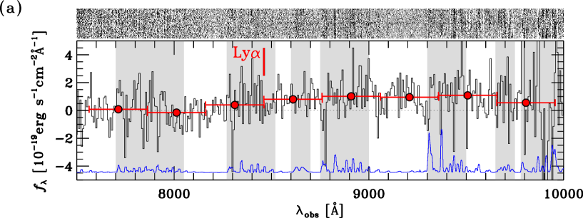
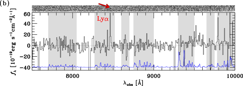
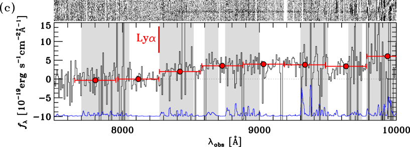
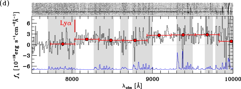
Figure 2: Optical spectra of $z\sim 6$ $i$-dropout galaxies: (a) HSC J090704+002624, (b) HSC J100332+024552, (c) HSC J084818+004509, and (d) HSC J084021+010311. In each figure, the top panel shows the two-dimensional spectrum (black is positive) and the bottom panel shows the one-dimensional spectrum. In the top panel, our dropout galaxy is located at the center in the spatial direction. The size along the spatial axis is $12\farcs 7$ for (a)–(c) and $16\farcs 8$ for (d). In the spectrum of (b), the Ly$\alpha$ emission line is marked with a red arrow. In the bottom panel, the object spectrum is shown with black histogram. All the spectra are smoothed by $8$–$9$ pixels ($11$–$12$ Å). For the sources without Ly$\alpha$ in emission, we also plot the averaged spectra over about $300$ Å bins with red filled circles and mark the wavelength of the Ly$\alpha$ transition with red vertical solid lines. The horizontal dotted line corresponds to zero flux density. The sky spectrum with an arbitrary normalization is plotted in blue (offset from zero).

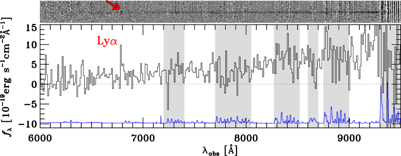
Figure 3: Same as Figure 2, but for a $z\sim 5$ $r$-dropout galaxy, HSC J021930–050915. In the top panel, the size along the spatial axis is $12\farcs 7$.

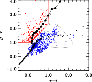
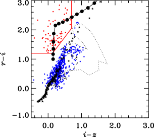
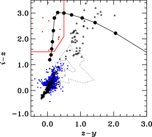
Figure 4: Left: $g-r$ vs. $r-i$ two color diagram. The red circles are the spectroscopically identified galaxies in our $g$-dropout sample, and the blue circles are sources in the UD-COSMOS field with spectroscopic redshifts of $z=0-3$ measured by the VVDS survey. The black solid line indicates the track of young star-forming galaxy spectra produced with the Bruzual & Charlot (2003) model. The black filled circles on the black solid line show their redshift from $z=3.1$ to $z=4.5$ with an interval of $\Delta z=0.1$. The red solid lines show the color selection criteria for our $g$-dropouts. The dotted, dashed, and dot-dashed lines are typical spectra of elliptical, Sbc, and irregular galaxies (Coleman et al., 1980) redshifted from $z=0$ to $z=2$. The filled and open stars indicate Galactic stars taken from Gunn & Stryker (1983) and L /T dwarfs from Knapp et al. (2004). Middle: $r-i$ vs. $i-z$ two color diagram. The red circles are the spectroscopically identified galaxies in our $r$-dropout sample. The redshift range of the black filled circles are from $z=4.2$ to $z=5.5$. The redshift ranges of the dotted, dashed, and dot-dashed lines are from $z=0$ to $z=3$. The other symbols are the same as in the left panel. Right: $i-z$ vs. $z-y$ two color diagram. The red circles are the spectroscopically identified galaxies in our $i$-dropout sample. The redshift range of the black filled circles are from $z=5.4$ to $z=6.5$. The other symbols are the same as in the middle panel.

In our samples, five sources are identified through our spectroscopic follow-up observations with FOCAS (Section 2.2). We find the five LBG candidates, HSC J090704+002624, HSC J100332+024552, HSC J084818+004509, HSC J084021+010311, and HSC J021930–050915, are real high-$z$ galaxies at $z\simeq 5.96$, $z=5.957$, $z\simeq 5.80$, $z\simeq 5.61$, and $z=4.580$. The first four galaxies are included in our $i$-dropout sample, and the last one is in our $r$-dropout sample. The first and the last three galaxies were selected for our follow-up targets because they are relatively bright among sources in our samples that could be targeted during our observing runs and had not been spectroscopically observed. The second galaxy was a mask filler source that was randomly chosen from our $i$-dropout candidates within the field-of-view of FOCAS centered on a primary target, a bright LAE. Figures 2 and 3 show the one-dimensional and two-dimensional spectra of the five identified galaxies. For HSC J100332+024552 and HSC J021930–050915, we detect an emission line that shows an asymmetric profile with a steeply rising edge at the shorter wavelength of the peak and a slowly decaying red tail, which are characteristic features of Ly$\alpha$ at high redshift (Kashikawa et al., 2006; Shimasaku et al., 2006). Their redshifts are determined based on the Ly$\alpha$ emission line. For the other three sources, their Ly$\alpha$ break feature and low-S/N absorption line features in their continua are used for their redshift determinations, although their uncertainties are relatively large. Since we have taken only two exposures for HSC J084818+004509 due to a technical problem in our observations, the reduced spectrum is severely affected by cosmic rays. This source has also been observed with LDSS3. However, the number of exposures with LDSS3 is also only two and it is difficult to remove cosmic rays in its reduced spectrum, although the Ly$\alpha$ break feature in its continuum is confirmed. Note that HSC J084818+004509 has been reported as a $z=5.78$ galaxy by the Subaru high-$z$ exploration of low-luminosity quasars (SHELLQs) survey (Matsuoka et al., 2016), whose redshift determination result is broadly consistent with our result. Although these five sources are likely to be high-$z$ galaxies because of these observational results, it should be noted that it is difficult to completely rule out the possibilities that they are foreground sources such as Galactic brown dwarfs based on these low-S/N spectra. The nature of these sources will be checked by future follow-up observations.

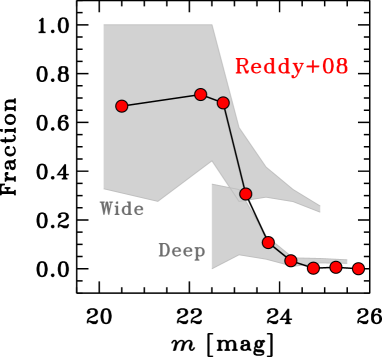
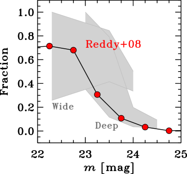
Figure 5: Estimated contamination fractions as a function of apparent magnitude for our $g$-dropout (top) and $r$-dropout (bottom) samples. The gray shaded regions represent the $1\sigma$ uncertainties of the estimated contamination fractions for the Wide and Deep layers. For the apparent magnitude, $i$- and $z$-band magnitudes are used for $g$-dropouts and $r$-dropouts, respectively. The red filled circles are the results of Reddy et al. (2008) for their LBG sample.

Estimated contamination fractions for the $z\sim 4$ and $z\sim 5$ samples selected from the W- and D-layer data. magnitude fraction magnitude fraction $z\sim 4$ in D $z\sim 5$ in D 22.5 $0.08^{+0.27}_{-0.08}$ 23.0 $0.94^{+0.06}_{-0.59}$ 23.1 $0.16^{+0.17}_{-0.10}$ 23.5 $0.34^{+0.46}_{-0.22}$ 23.7 $0.08^{+0.05}_{-0.04}$ 24.0 $0.10^{+0.10}_{-0.06}$ 24.3 $0.03^{+0.02}_{-0.02}$ 24.5 $0.06^{+0.04}_{-0.03}$ 24.9 $0.03^{+0.01}_{-0.01}$ — — 25.5 $0.03^{+0.01}_{-0.01}$ — — $z\sim 4$ in W $z\sim 5$ in W 20.1 $0.91^{+0.09}_{-0.59}$ 22.3 $0.73^{+0.27}_{-0.47}$ 21.3 $0.79^{+0.21}_{-0.51}$ 23.5 $0.59^{+0.25}_{-0.18}$ 22.5 $0.68^{+0.32}_{-0.23}$ 24.0 $0.41^{+0.09}_{-0.08}$ 23.1 $0.41^{+0.17}_{-0.13}$ — — 23.7 $0.35^{+0.07}_{-0.06}$ — — 24.3 $0.30^{+0.03}_{-0.02}$ — — 24.9 $0.24^{+0.01}_{-0.01}$ — —

In addition, we incorporate the results of our spectroscopic observations for high-$z$ galaxies with Magellan/IMACS (Section 2.2). We also check the spectroscopic catalogs shown in other studies (Saito et al. (2008); Ouchi et al. (2008); Willott et al. (2010a); Curtis-Lake et al. (2012); Masters et al. (2012); Mallery et al. (2012); Willott et al. (2013); Le Fèvre et al. (2013); Kashikawa et al. (2015); Kriek et al. (2015); Wang et al. (2016); Toshikawa et al. (2016); Momcheva et al. (2016); Matsuoka et al. (2016); Pâris et al. (2017); Tasca et al. (2017); Yang et al. (2017); Masters et al. (2017); Matsuoka et al. (2017); Shibuya et al. (2017b); R. Higuchi et al. in preparation; see also Bañados et al. (2016)). We adopt their classifications between galaxies and AGNs in their catalogs. For the catalogs of the VIMOS VLT Deep Survey (VVDS; Le Fèvre et al. (2013)) and the VIMOS Ultra Deep Survey (VUDS; Tasca et al. (2017)), we take into account sources whose redshifts are $>70-75$% correct, i.e., sources with redshift reliability flags of 2, 3, 4, 9, 12, 13, 14, and 19. Here we focus on sources with spectroscopic redshifts $z_{\rm spec}>3$ in these catalogs. Our contamination estimates with sources at $z_{\rm spec}<3$ are presented in the next section.

In total, 358 dropouts in our sample have been spectroscopically identified by our observations and the other studies. Among these identified sources, 270 sources are found to be galaxies at $z_{\rm spec}>3$, and the other 88 sources are AGNs. These sources are listed in Table 2.2.

Figure 4 shows the distributions of the spectroscopically identified galaxies at $z_{\rm spec}>3$ in our dropout samples in the two-color diagrams. We also plot sources in the UD-COSMOS field with spectroscopic redshifts of $z_{\rm spec}<3$ that are measured by the VVDS. In addition, the tracks of model spectra of young star-forming galaxies that are produced with the stellar population synthesis code galaxev (Bruzual & Charlot, 2003) are shown. As model parameters a Salpeter initial mass function (Salpeter, 1955), an age of $70$ Myr after the initial star formation, and metallicity of $Z/Z_{\odot}=0.2$ are adopted. We use the Calzetti et al. (2000) dust extinction formula with reddening of $E(B-V)=0.16$. The IGM absorption is considered following the prescription of Madau (1995). The colors of the spectroscopically identified galaxies are broadly consistent with those expected from the model spectra.

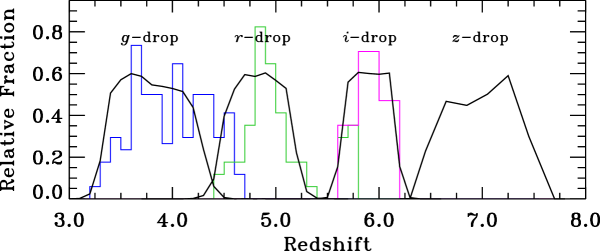
Figure 6: Selection completeness estimates for our $z\sim 4$, $z\sim 5$, $z\sim 6$, and $z\sim 7$ samples The black curves correspond to the results of our Monte Carlo calculations averaged over the W, D, and UD layers described in Section 3.3. The average redshifts of these samples are roughly $3.8$, $4.9$, $5.9$, and $6.9$. The blue, green, and magenta histograms are the redshift distributions of the spectroscopically identified galaxies in $g$-, $r$-, and $i$-dropout samples, respectively.

3.2 Contamination

Some foreground objects such as red galaxies at intermediate redshifts can satisfy our color criteria by photometric errors, although intrinsically they do not enter the color selection window. To estimate the numbers of such contaminants in our dropout samples, we use shallower HSC data of COSMOS that are created with a subset of the real HSC data for the UD-COSMOS field. We use two shallower data sets whose depths are comparable with those in the W layer and D layer. We assume that the UD-COSMOS data are sufficiently deep and the contamination rates in our dropout selections for the UD-COSMOS are small. First, we select objects which do not satisfy our selection criteria from the UD-COSMOS catalog. We then regard them as foreground interlopers in the W-layer-depth and D-layer-depth COSMOS samples if they satisfy our selection criteria for the W-layer and D-layer dropouts, respectively, and calculate their number counts. Based on comparisons between the surface number densities of interlopers and those of the selected dropouts, we estimate the fractions of foreground interlopers, which are shown in Figure 5 and Table 3.1. The fractions of foreground interlopers at magnitude fainter than $24.0$ mag are estimated to be less than about $10$% for the D-layer samples and less than about $30-40$% for the W-layer samples. At the brighter magnitude bins, our dropout samples in the wide and deep layers are more contaminated by the foreground interlopers. Note that similar results have been obtained by Reddy et al. (2008). We subtract the number counts of foreground interlopers from the number counts of our dropouts and consider both of the uncertainties in Section 4.1. For a sanity check, we derive the interloper fraction in the W-layer samples by using the spec-$z$ catalog of VVDS, which covers a small portion of our W-layer fields. Although the number of objects which are included in both our samples and the VVDS catalog is small, the interloper fraction for the $z\sim 4$ W-layer sample is estimated to be about 40%, which is consistent with the results estimated from the shallower HSC data.

For the $z\sim 6-7$ dropout samples, we cannot estimate the surface number densities of interlopers by adopting this method, since the number densities of such sources in the shallower depth COSMOS field data are too low. Instead, we make use of the spectroscopic observation results taken by our study as well as in the literature. Based on the spectroscopic redshift catalog created in Section 3.1, 31 sources in our $z\sim 6$ dropout sample are spectroscopically identified in our follow-up observations and in the other studies and all the sources are at $z>5.5$. Although it is unclear whether the other candidates are real high-$z$ sources or foreground interlopers, we assume that the contamination fraction of interlopers is negligibly small based on the limited spectroscopy results. For $z\sim 7$ dropout sample, none of our candidates have been followed up with spectroscopy. We will carry out follow-up spectroscopy for our $z$-dropout candidates in the near future.

It should be noted that our sample is contaminated not only by low-$z$ interlopers but also by high-$z$ AGNs. We take into account the AGN contamination in our samples in Section 4.

3.3 Selection Completeness

We estimate the selection completeness of our dropout galaxies by running a suite of Monte Carlo simulations with an input mock catalog of high-$z$ galaxies. In the mock catalog, the size distribution of galaxies follows recent results of galaxy log-normal size distributions and size-luminosity relations as a function of redshift based on Hubble legacy data sets (Shibuya et al. (2015); see also Oesch et al. (2010); Mosleh et al. (2012); Ono et al. (2013); Kawamata et al. (2015); Curtis-Lake et al. (2016); Ribeiro et al. (2016)). The Sersic index $n$ is fixed at $n=1.5$, which is also suggested from the results of Shibuya et al. (2015). A uniform distribution of the intrinsic ellipticities in the range of $0.0$–$0.8$ is assumed, since the observational results of $z\sim 3-5$ dropout galaxies have roughly uniform distributions (Ravindranath et al., 2006). Position angles are randomly chosen. To produce galaxy SEDs, we use the stellar population synthesis model of galaxev (Bruzual & Charlot, 2003). We adopt the Salpeter initial mass function (Salpeter, 1955) with lower and upper mass cutoffs of $0.1M_{\odot}$ and $100M_{\odot}$, a constant rate of star formation, age of $25$ Myr, metallicity of $Z/Z_{\odot}=0.2$, and Calzetti et al. (2000) dust extinction ranging from $E(B-V)=0.0$–$0.4$ so that we can cover from very blue continua with $\beta\simeq-3.0$ to moderately red ones with $\beta\simeq-1.0$. The IGM absorption is taken into account by using the prescription of Madau (1995).

Different simulations are carried out for the W, D, and UD layers by using the SynPipe software (Huang et al., 2017; Murata et al., 2017), which utilizes GalSim v1.4 (Rowe et al., 2015) and the HSC pipeline. We insert large numbers of artificial sources into HSC images of individual CCDs at the single exposure level. Next we stack the single exposure images and create source catalogs in the same manner as the real ones. We then select high-$z$ galaxy candidates with the same selection criteria and calculate the selection completeness as a function of magnitude and redshift, $C(m,z)$, averaged over UV slope $\beta$ weighted with the $\beta$ distribution of Bouwens et al. (2014). For the $\beta$ distribution of very bright sources at $M_{\rm UV}\lesssim-22$ mag where Bouwens et al. (2014) do not probe, we extrapolate their results for fainter magnitudes.

Figure 6 shows the results of our selection completeness estimates as a function of redshift. The average redshift values are roughly $z\sim 3.8$ for $g$-dropouts, $z\sim 4.9$ for $r$-dropouts, $z\sim 5.9$ for $i$-dropouts, and $z\sim 6.9$ for $z$-dropouts. In Figure 6, we also show the redshift distributions of the spectroscopically identified galaxies in our samples (Section 3.1). The redshift distributions of the spectroscopically identified galaxies are broadly consistent with the results of our selection completeness simulations, although the distributions of the spectroscopically identified galaxies in the $g$- and $r$-dropout samples appear to be shifted toward slightly higher redshift. This is probably because the spectroscopically identified galaxies are biased to ones with strong Ly$\alpha$ emission. In particular, the redshift distribution of the spectroscopically identified $r$-dropouts has a secondary peak at around $z=5.7$, which is caused by $z=5.7$ Ly$\alpha$ emitters found by Subaru Suprime-Cam and HSC narrowband surveys in the literature.

4 Results and Discussion

4.1 The UV Luminosity Functions

Estimated galaxy UV LFs at $z\sim 4$, $z\sim 5$, $z\sim 6$, and $z\sim 7$ based on the HSC SSP data. $M_{\rm UV}$ $\Phi$ $M_{\rm UV}$ $\Phi$ (mag) ($10^{-4}$ mag^-1 Mpc^-3) (mag) ($10^{-4}$ mag^-1 Mpc^-3) $z\sim 4$ $z\sim 6$ $-23.837$ $0.00055^{+0.00156}_{-0.00055}$ $-24.244$ $0.00001^{+0.00019}_{-0.00001}$ $-23.637$ $0.00113^{+0.00205}_{-0.00103}$ $-23.944$ $0.00002^{+0.00019}_{-0.00002}$ $-23.437$ $0.00325^{+0.00380}_{-0.00197}$ $-23.644$ $0.00007^{+0.00026}_{-0.00007}$ $-23.237$ $0.00630^{+0.00474}_{-0.00286}$ $-23.344$ $0.00016^{+0.00025}_{-0.00011}$ $-23.037$ $0.00885^{+0.00490}_{-0.00333}$ $-23.044$ $0.00147^{+0.00107}_{-0.00066}$ $-22.837$ $0.02171^{+0.00827}_{-0.00702}$ $-22.744$ $0.00621^{+0.00292}_{-0.00231}$ $-22.637$ $0.04771^{+0.01277}_{-0.01343}$ $-22.444$ $0.02553^{+0.00360}_{-0.00243}$ $-22.437$ $0.10648^{+0.02046}_{-0.02616}$ $-22.144$ $0.05615^{+0.01242}_{-0.00777}$ $-22.237$ $0.19365^{+0.02885}_{-0.04072}$ $-21.844$ $0.21313^{+0.05322}_{-0.04056}$ $-22.037$ $0.37561^{+0.04174}_{-0.06703}$ $-21.544$ $0.49479^{+0.11521}_{-0.08826}$ $-21.837$ $0.72645^{+0.05566}_{-0.10819}$ — — $-21.637$ $1.30260^{+0.05961}_{-0.15856}$ — — $-21.437$ $2.27743^{+0.05760}_{-0.23933}$ — — $-21.237$ $3.71089^{+0.07428}_{-0.40147}$ — — $-21.037$ $5.60696^{+0.08491}_{-0.62452}$ — — $-20.837$ $7.96770^{+0.10421}_{-0.91524}$ — — $-20.637$ $10.05840^{+0.10550}_{-1.18857}$ — — $-20.437$ $12.74950^{+0.25563}_{-0.24866}$ — — $-20.237$ $16.72980^{+0.30374}_{-0.29621}$ — — $-20.037$ $23.61950^{+0.41061}_{-0.40085}$ — — $-19.837$ $29.82960^{+0.57881}_{-0.56363}$ — — $z\sim 5$ $z\sim 7$ $-24.241$ $0.00003^{+0.00013}_{-0.00003}$ $-24.165$ $0.00001^{+0.00019}_{-0.00001}$ $-23.491$ $0.00012^{+0.00190}_{-0.00012}$ $-23.665$ $0.00010^{+0.00039}_{-0.00009}$ $-22.991$ $0.00397^{+0.00422}_{-0.00258}$ $-23.165$ $0.00091^{+0.00080}_{-0.00044}$ $-22.741$ $0.02156^{+0.00813}_{-0.00692}$ — — $-22.491$ $0.06576^{+0.01501}_{-0.01736}$ — — $-22.241$ $0.16906^{+0.02681}_{-0.03629}$ — — $-21.991$ $0.40066^{+0.04266}_{-0.06929}$ — — $-21.741$ $0.81996^{+0.05653}_{-0.11351}$ — — $-21.491$ $1.44029^{+0.09020}_{-0.16802}$ — — $-21.241$ $2.50578^{+0.12027}_{-0.28970}$ — — $-20.991$ $3.91303^{+0.15802}_{-0.46063}$ — —

We derive the rest-frame UV luminosity functions of $z\sim 4-7$ galaxies by applying the effective volume method (Steidel et al., 1999). Based on the results of the selection completeness simulations, we estimate the effective survey volume per unit area as a function of apparent magnitude,

$$V_{\rm eff}(m)=\int C(m,z)\frac{dV(z)}{dz}dz,$$ (11)

where $C(m,z)$ is the selection completeness estimated in Section 3.3, i.e., the probability that a galaxy with apparent magnitude $m$ at redshift $z$ is detected and satisfies the selection criteria, and $dV(z)/dz$ is the differential comoving volume as a function of redshift (e.g., Hogg (1999)).

The space number densities of dropouts that are corrected for incompleteness and contamination effects are obtained by calculating

$$\psi(m)=\frac{n_{\rm raw}(m)-n_{\rm con}(m)}{V_{\rm eff}(m)},$$ (12)

where $n_{\rm raw}(m)$ is the surface number density of selected dropouts in an apparent magnitude bin of $m$, and $n_{\rm con}(m)$ is the surface number density of interlopers in the magnitude bin estimated in Section 3.2. To calculate the surface number densities, we use the effective area values summarized in Table 1. The $1\sigma$ uncertainties are calculated by taking account of Poisson confidence limits (Gehrels, 1986) on the numbers of the sources. To calculate the $1\sigma$ uncertainties of the space number densities of dropouts, we consider the uncertainties of the surface number densities of selected dropouts and those of interlopers. We restrict our analysis for the $z\sim 4-5$ D- and W-layer samples to the magnitude ranges where the contamination rate estimates are available. Note that the $z\sim 4$ UD-layer sample includes several very bright candidates with magnitude brighter than $22.0$ mag. However, three of them have been spectroscopically observed and all of the three are at $z_{\rm spec}<1$ (Lilly et al., 2009), while many fainter sources have been identified at $z_{\rm spec}>3$ as checked in Section 3.1. Although the number of observed very bright sources is small, we do not use dropout candidates with magnitude brighter than $22.0$ mag in the $z\sim 4$ UD-layer sample.

We convert the number densities of dropouts as a function of apparent magnitude, $\psi(m)$, into the UV LFs, $\Phi[M_{\rm UV}(m)]$, i.e., the number densities of dropouts as a function of rest-frame UV absolute magnitude. We calculate the absolute UV magnitudes of dropouts from their apparent magnitudes using their average redshifts $\bar{z}$:

$$M_{\rm UV}=m+2.5\log(1+\bar{z})-5\log\left(\frac{d_{\rm L}(\bar{z})}{10\,{\rm pc}}\right)+(m_{\rm UV}-m),$$ (13)

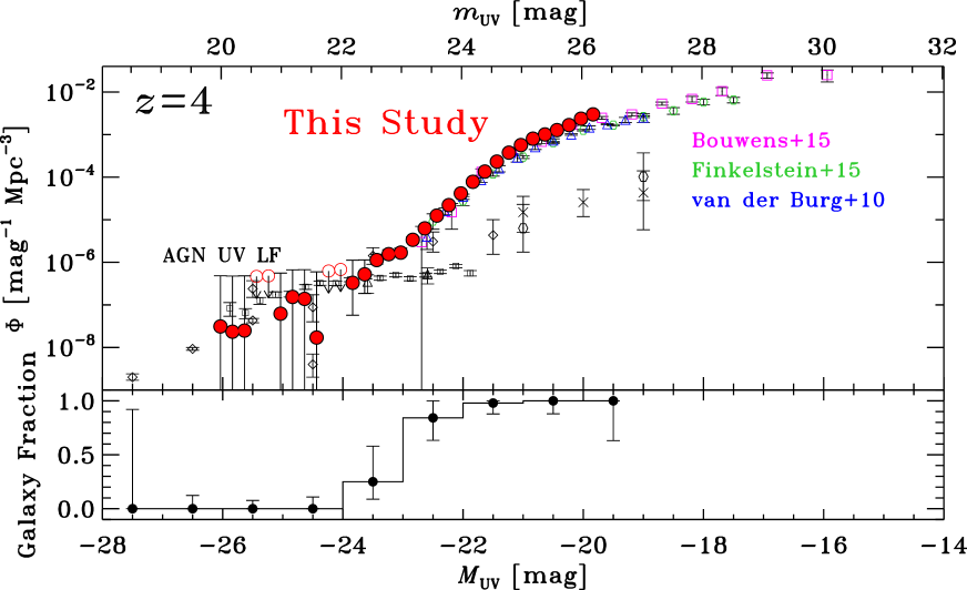
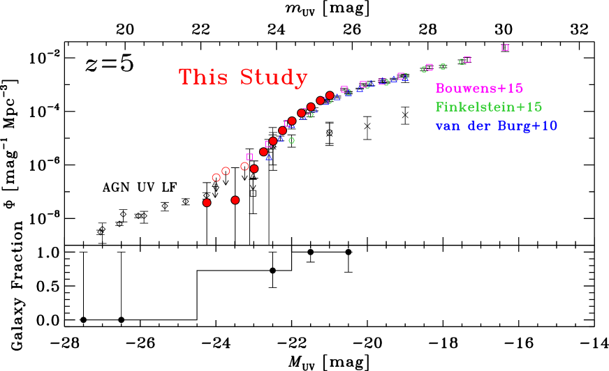
Figure 7: Top: rest-frame UV luminosity functions of dropouts before quasar contamination correction at $z\sim 4$ and $z\sim 5$. The red circles show our results based on the HSC SSP survey data. The red open circles with a downward arrow denote the $1\sigma$ upper limits. For comparison, we also show previous results for galaxies taken from 2015ApJ…803…34B (2015ApJ…803…34B; open magenta squares) at $z\sim 4-5$, 2015ApJ…810…71F (2015ApJ…810…71F; open green hexagons) at $z\sim 4-5$, and 2010AA…523A..74V (2010AA…523A..74V; open blue triangles) at $z\sim 4-5$. Our LF estimates are broadly in agreement with previous results in the magnitude range where previous results are available. In addition, we plot previous results for quasars taken from 2011ApJ…728L..26G (2011ApJ…728L..26G; open black diamonds) at $z\sim 4$, 2015AA…578A..83G (2015AA…578A..83G; black crosses) at $z\sim 4-5$, 2017arXiv170407750P (2017arXiv170407750P; open black hexagons) at $z\sim 4-5$, 2016ApJ…832..208N (2016ApJ…832..208N; open black triangle) at $z\sim 4-5$, 2017arXiv170405996A (2017arXiv170405996A; open black squares) at $z=4$, 2013ApJ…768..105M (2013ApJ…768..105M; open black diamonds) at $z\sim 5$, and 2012ApJ…756..160I (2012ApJ…756..160I; open black squares) at $z\sim 5$. Bottom: fraction of galaxies in our $z\sim 4-5$ dropout samples based on spectroscopy results. For the denominator of the fraction, the sum of the numbers of galaxies and quasars is used.

where $d_{\rm L}$ is the luminosity distance in units of parsecs and $(m_{\rm UV}-m)$ is the $K$-correction term between the magnitude at rest-frame UV and the magnitude in the bandpass that we use. We set the $K$-correction term to be $0$ by assuming that dropout galaxies have flat UV continua, i.e., constant $f_{\nu}$ in the rest-frame UV (e.g., Figure 3 of Sawicki & Thompson (2006) and Figure 7 of van der Burg et al. (2010)). For the apparent magnitude $m$, we use $i$-band magnitudes for $g$-dropouts, $z$-band magnitudes for $r$- and $i$-dropouts, and $y$-band magnitudes for $z$-dropouts. The central wavelength of the $i$-band corresponds to $\sim 1600$ Å in the rest-frame of $g$-dropouts, and that of the $z$-band is $\sim 1300-1500$ Å in the rest-frame of $r$- and $i$-dropouts, on average. Note that the $y$-band probes slightly shorter wavelength in the rest-frame of $z$-dropouts, about $1230$ Å.

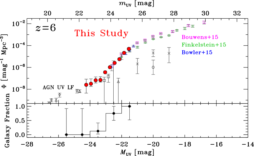
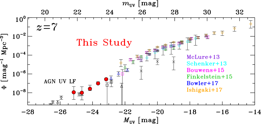
Figure 8: Same as Figure 7, but for $z\sim 6$ and $z\sim 7$. For comparison, we also show previous results for galaxies taken from 2013MNRAS.432.2696M (2013MNRAS.432.2696M; open purple pendagons) at $z\sim 7$, 2013ApJ…768..196S (2013ApJ…768..196S; open cyan circles) at $z\sim 7$, 2015ApJ…803…34B (2015ApJ…803…34B; open magenta squares) at $z\sim 6-7$, 2015ApJ…810…71F (2015ApJ…810…71F; open green hexagons) at $z\sim 6-7$, 2015MNRAS.452.1817B (2015MNRAS.452.1817B; open blue triangles) at $z\sim 6$, 2017MNRAS.466.3612B (2017MNRAS.466.3612B; open blue triangles) at $z\sim 7$, and 2017arXiv170204867I (2017arXiv170204867I; open orange diamonds) at $z\sim 7$. In addition, we plot previous results for quasars taken from 2015AA…578A..83G (2015AA…578A..83G; black crosses) at $z\sim 6$, 2017arXiv170407750P (2017arXiv170407750P; open black hexagons) at $z\sim 6$, 2010AJ….139..906W (2010AJ….139..906W; open black triangles) at $z\sim 6$, 2015ApJ…798…28K (2015ApJ…798…28K; open black squares) at $z\sim 6$, and 2016ApJ…833..222J (2016ApJ…833..222J; open black diamonds) at $z\sim 6$.

The top panel of Figure 7 shows our derived LF for dropouts at $z\sim 4$ and those taken from the previous galaxy work of Bouwens et al. (2015) and Finkelstein et al. (2015), which are based on the Hubble legacy survey data, and that of van der Burg et al. (2010), which is based on the CFHT deep legacy survey data. The previous studies have derived their UV LF estimates in the UV magnitude range of $M_{\rm UV}>-23$ mag. Our results are broadly consistent with the previous results in this magnitude range. However, at $M_{\rm UV}<-23$ mag, where no previous high-$z$ galaxy studies have probed, our results appear to have a hump and follow a shallower slope than the extrapolation of the exponential cutoff from the fainter bins. Figure 7 also shows our LF results for the $z\sim 5$ dropout sample and the results of the previous galaxy studies. We find that the situation is similar to that for the $z\sim 4$ dropout sample. In Figure 8, we present the results of our LF estimates for the $z\sim 6-7$ dropout samples. For $z\sim 6$, we also plot the previous results taken from Bouwens et al. (2015), Finkelstein et al. (2015), and Bowler et al. (2015). For $z\sim 7$, the previous estimates by McLure et al. (2013), Schenker et al. (2013), Bouwens et al. (2015), Finkelstein et al. (2015), Bowler et al. (2017), and Ishigaki et al. (2017) are shown for comparison. These previous work has presented their estimates in the magnitude range of $M_{\rm UV}>-22.5$ ($-23.0$) mag at $z\sim 6$ ($z\sim 7$). Our results are in good agreement with the previous results in these magnitude ranges. However, at the brighter magnitude ranges, our LF results seem to have a hump compared to the simple extrapolation of the exponentially declining shape. Note that the effect of the Eddington bias (Eddington, 1913), which can cause an apparent increase of the number of bright sources due to photometric scatter from sources in fainter bins, should be small at these bright-end hump features. This is because their magnitude ranges are much brighter than the limiting magnitudes of the samples.

To investigate the bright-end hump features, we plot the UV LFs of AGNs taken from the literature in Figure 7. We find that the bright-end hump features in our LF results for dropouts are broadly consistent with the UV LFs of AGNs obtained by Glikman et al. (2011). Our LF results are also consistent with those of Akiyama et al. (2017) at the very bright end of $M_{\rm UV}\sim-25$ mag, but our results are larger at $M_{\rm UV}\sim-23$ mag than their results as well as those of Niida et al. (2016). This is probably because they focus on $z\sim 4$ quasars with stellar morphology while the selection of ours and Glikman et al. (2011) can also identify galaxies with faint AGNs whose morphology is extended (see also Akiyama et al. (2017)). In Figure 7, we also compare our bright-end LF results with those of AGNs at $z\sim 5$ obtained by Ikeda et al. (2012), McGreer et al. (2013), and Niida et al. (2016). Although the uncertainties of our estimates are large, our results are in agreement with these AGN results. In addition, Figure 8 shows that our bright-end LF results for dropouts are broadly consistent with those of AGNs at $z\sim 6$ taken from Willott et al. (2010b), Kashikawa et al. (2015), and Jiang et al. (2016).

In our dropout selection, we probe redshifted Ly$\alpha$ break features of high-$z$ galaxies. However, high-$z$ AGNs also have similar Ly$\alpha$ break features. It is thus expected that our dropout sample is contaminated by AGNs (e.g., for $i$-dropout selection, see Figure 1 of Matsuoka et al. (2016)). Actually, as described in Section 3.1, our dropout samples include spectroscopically confirmed AGNs. Based on our spectroscopy results as well as those in the literature, we derive the galaxy fraction of spectroscopically confirmed dropouts, i.e., the number of spectroscopically confirmed high-$z$ galaxies divided by the sum of the numbers of spectroscopically confirmed high-$z$ galaxies and AGNs, in our $z\sim 4-6$ samples in each magnitude bin (Figures 7 and 8). As shown in Figure 7, the $z\sim 4$ galaxy fraction is smaller than $20$% at $M_{\rm UV}<-23$ mag, but it increases with increasing magnitude and it reaches about $100$% at $M_{\rm UV}>-22$ mag. Similarly, in Figure 8, the galaxy fraction for the $z\sim 6$ sample is less (more) than $50$% at $M_{\rm UV}<-23$ mag ($M_{\rm UV}>-23$ mag). These results suggest that our bright-end LF estimates are significantly contaminated by AGNs. The very wide area of the HSC SSP allows us to bridge the UV LFs of high-$z$ galaxies and AGNs, both of which can be selected with redshifted Ly$\alpha$ break features. Note that we also show the results of the faint end of the AGN UV LFs (Giallongo et al. (2015); Parsa et al. (2017)) in the magnitude range of $M_{\rm UV}\gtrsim-22$ mag in Figures 7 and 8. We find that our results are much larger than their results, which also suggests that the AGN contamination is not significant in this faint magnitude range.

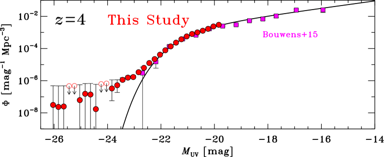
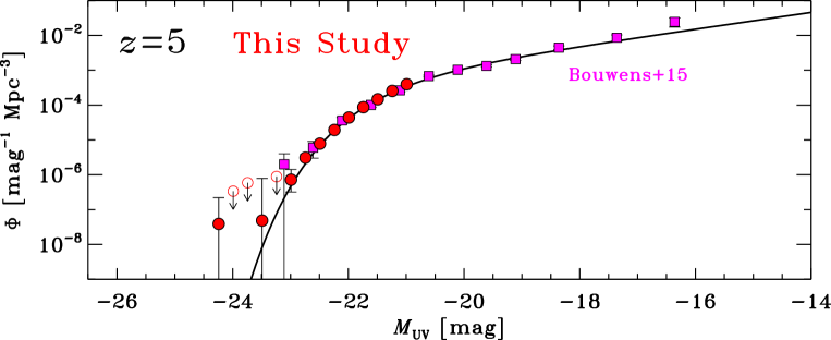
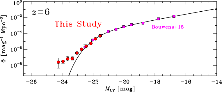
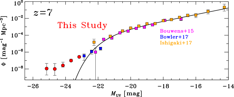
Figure 9: Rest-frame UV luminosity functions of dropouts at $z\sim 4$, $z\sim 5$, $z\sim 6$, and $z\sim 7$ from top to bottom. The red circles show our results based on the HSC SSP survey data. The red open circles with a downward arrow are the $1\sigma$ upper limits. For comparison, we also show previous results for galaxies taken from 2015ApJ…803…34B (2015ApJ…803…34B; filled magenta squares) at $z\sim 4-7$, 2017MNRAS.466.3612B (2017MNRAS.466.3612B; filled blue squares) at $z\sim 7$, and 2017arXiv170204867I (2017arXiv170204867I; filled orange squares) at $z\sim 7$. The solid lines are the best-fit Schechter functions.

Because it is not easy to distinguish galaxies from AGNs in our dropout samples solely based on the ground-based optical imaging data, we first investigate the shape of the UV LFs of dropouts by focusing on the magnitude range where the galaxy fraction is large. Figure 9 shows the UV LFs of dropouts at $z\sim 4-7$ based on our Subaru HSC results, previous Hubble results (Bouwens et al. (2015); Ishigaki et al. (2017)), and other ground-based telescope results (Bowler et al., 2017). The combination of our results with the previous work reveals the shapes of the UV LFs for high-$z$ dropout sources in a very wide magnitude range of $-26\lesssim M_{\rm UV}\lesssim-14$ mag for the first time. Our wide area survey reveals that the UV LFs of dropouts have bright end humps that are related to the significant contribution of light from AGNs. To characterize the UV LFs of dropout galaxies, we focus on the LF estimates at $M_{\rm UV}>-23$ mag, where the galaxy fraction is significantly large. We fit a Schechter function (Schechter, 1976) to the data points,

$$\phi(L)dL=\phi^{\ast}\left(\frac{L}{L^{\ast}}\right)^{\alpha}\exp\left(-\frac{L}{L^{\ast}}\right)d\left(\frac{L}{L^{\ast}}\right),$$ (14)

where $\phi^{\ast}$ is the overall normalization, $L^{\ast}$ is the characteristic luminosity, and $\alpha$ is the faint-end slope. We define a Schechter function expressed in terms of absolute magnitude $\Phi(M_{\rm UV})$ as $\phi(L)dL=\Phi(M_{\rm UV})dM_{\rm UV}$, i.e.,

$$\Phi(M_{\rm UV}) = \frac{\ln 10}{2.5}\phi^{\ast}10^{-0.4(M_{\rm UV}-M_{\rm UV}^{\ast})(\alpha+1)}$$ (15)

$$\times\exp\left(-10^{-0.4(M_{\rm UV}-M_{\rm UV}^{\ast})}\right),$$

where $M^{\ast}_{\rm UV}$ is the characteristic magnitude. We fit this function to the observed LFs derived from the results of our observations and the previous Hubble results of Bouwens et al. (2015) and Ishigaki et al. (2017). Varying the three parameters, we search for the best-fit set of ($\phi^{\ast}$, $M^{\ast}_{\rm UV}$, $\alpha$) that minimizes $\chi^{2}$. The best-fit parameters are summarized in Table 4.2 and the best-fit Schechter function is plotted in Figure 9.

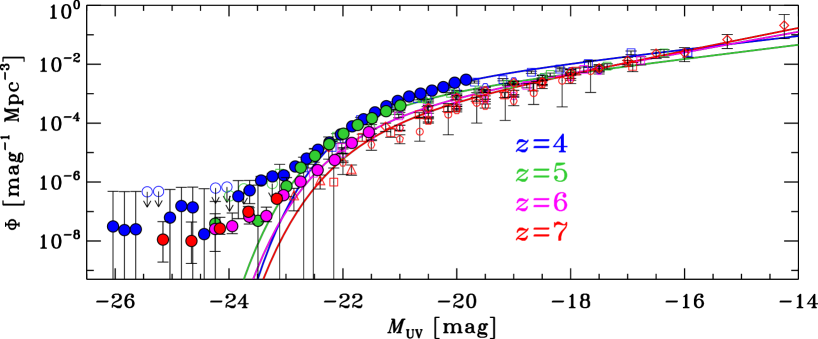
Figure 10: Rest-frame UV luminosity functions of dropouts and the best-fit Schechter functions at $z\sim 4$ (blue), $z\sim 5$ (green), $z\sim 6$ (magenta), and $z\sim 7$ (red). The filled circles and open circles with an arrow correspond to our results, and the pentagons, the small open circles, the squares, the hexagons, the triangles, and the diamonds are the results of McLure et al. (2013), Schenker et al. (2013), Bouwens et al. (2015), Finkelstein et al. (2015), Bowler et al. (2017), and Ishigaki et al. (2017), respectively.

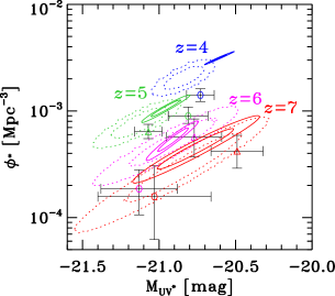
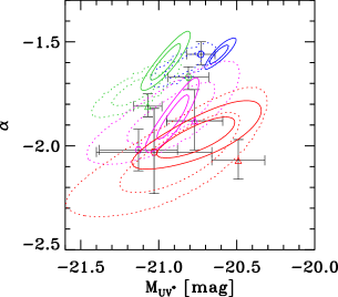
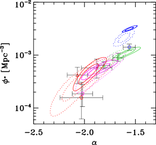
Figure 11: $1\sigma$ and $2\sigma$ confidence intervals on the Schechter parameters, $M_{\rm UV}^{\ast}$, $\phi^{\ast}$, and $\alpha$. The blue, green, magenta, and red solid contours correspond to our results for the galaxy UV LFs at $z\sim 4$, $z\sim 5$, $z\sim 6$, and $z\sim 7$, respectively. The dotted contours correspond to the results of Bouwens et al. (2015). The hexagons show the results of Finkelstein et al. (2015) and the triangles are those of Bowler et al. (2015) and Bowler et al. (2017).

Figure 10 summarizes the UV LF estimates at $z\sim 4-7$ and their best-fit Schechter functions. In Figure 11, we show the $1\sigma$ and $2\sigma$ confidence intervals for the combinations of the Schechter parameters. We find that $M_{\rm UV}^{\ast}$ shows little evolution while the other two parameters decrease with increasing redshift as already pointed out in the previous work (e.g., Bouwens et al. (2015); Bowler et al. (2015); Finkelstein et al. (2015)).

Note that there are on-going projects in our HSC SSP collaboration to search for high-$z$ quasars by using selection techniques that are optimized for quasars. The exact shapes of the quasar UV LFs at $z\sim 4$, $z\sim 5$, and $z\sim 6-7$ are presented in Akiyama et al. (2017), M. Niida et al. in preparation, and Y. Matsuoka et al. in preparation, respectively.

4.2 The Galaxy UV Luminosity Functions

In what follows, we estimate the galaxy UV LFs in as wide a magnitude range as possible by taking into account the contributions of AGNs in our LF estimates, although the associated uncertainties are not small. To subtract the AGN contributions, we take advantage of the galaxy fraction estimates based on the spectroscopy results shown in Figures 7 and 8; we multiply the UV LFs by the spectroscopic galaxy fraction, both of which are derived in Section 4.1. Since the number of spectroscopically confirmed sources in our $z\sim 5$ and $z\sim 7$ samples are not large, we apply the same galaxy fraction values for $z\sim 5$ ($z\sim 7$) as those for the $z\sim 4$ ($z\sim 6$) sample, assuming that the galaxy fraction has little evolution.

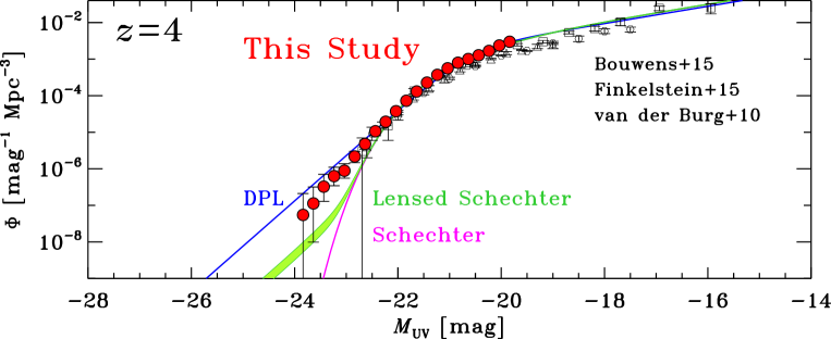
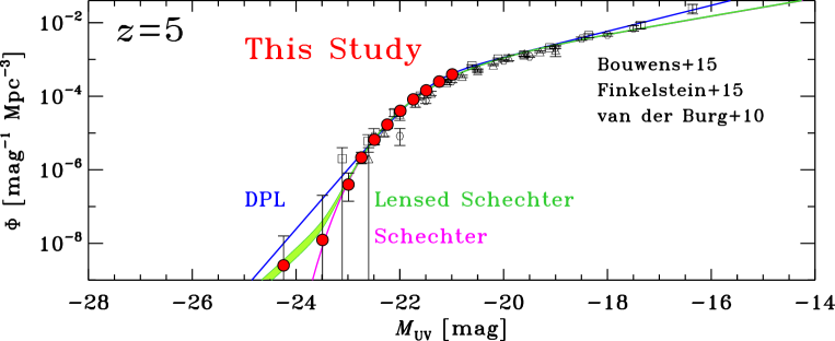
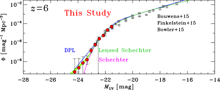
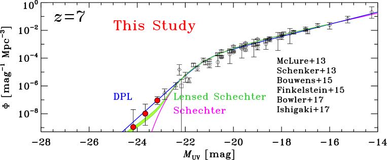
Figure 12: Rest-frame UV luminosity functions of galaxies that take into account quasar contamination correction at $z\sim 4$, $z\sim 5$, $z\sim 6$, and $z\sim 7$ from top to bottom. The green shaded region corresponds to the best-fit Schechter functions that take into account the effect of gravitational lensing with the two cases of the optical depth estimates (Takahashi et al., 2011; Barone-Nugent et al., 2015). The magenta curve is the best-fit Schechter function without considering the lensing effect and the blue curve is the best-fit DPL function. For comparison, we also show previous results for galaxies taken from 2013MNRAS.432.2696M (2013MNRAS.432.2696M; open pendagons) at $z\sim 7$, 2013ApJ…768..196S (2013ApJ…768..196S; open circles) at $z\sim 7$, 2015ApJ…803…34B (2015ApJ…803…34B; open squares) at $z\sim 4-7$, 2015ApJ…810…71F (2015ApJ…810…71F; open hexagons) at $z\sim 4-7$, 2017MNRAS.466.3612B (2017MNRAS.466.3612B; open triangles) at $z\sim 7$, and 2017arXiv170204867I (2017arXiv170204867I; open diamonds) at $z\sim 7$.

Figure 12 and Table 4.1 show our estimates of the galaxy UV LFs from $z\sim 4$ to $z\sim 7$. We confirm that our results are consistent with the previous results in the UV magnitude range fainter than $-23$ mag, as is also the case with our results before considering the contribution of AGNs. This is because the number densities of AGNs are negligibly small compared with galaxies in this magnitude range. In the brighter magnitude range of $M_{\rm UV}<-23$ mag, we find that our LF estimates for $z\sim 4$, $6$, and $7$ still appear to have a hump, although the uncertainties are large. To characterize the derived galaxy UV LFs, we compare the following three functions.

One form is a Schechter function (Equation 15). We adopt the best-fit Schechter functions that are obtained for the magnitude range where the galaxy fraction is large (Section 4.1). Table 4.2 summarizes the adopted parameter values and the reduced $\chi^{2}$.

Another functional form is a double power-law (DPL) function (e.g., Bowler et al. (2012)),

$$\phi(L)dL=\phi^{\ast}\left[\left(\frac{L}{L^{\ast}}\right)^{-\alpha}+\left(\frac{L}{L^{\ast}}\right)^{-\beta}\right]^{-1}\frac{dL}{L^{\ast}},$$ (16)

where the definitions of $\phi^{\ast}$, $M^{\ast}_{\rm UV}$, and $\alpha$ are the same as those in Equation (15), and $\beta$ is the bright-end power-law slope. We define a DPL function as a function of absolute magnitude $\Phi(M_{\rm UV})$ as $\phi(L)dL=\Phi(M_{\rm UV})dM_{\rm UV}$,

$$\Phi(M_{\rm UV}) = \frac{\ln 10}{2.5}\phi^{\ast}$$ (17)

$$\times\left[10^{0.4(\alpha+1)(M_{\rm UV}-M_{\rm UV}^{\ast})}+10^{0.4(\beta+1)(M_{\rm UV}-M_{\rm UV}^{\ast})}\right]^{-1}.$$

We derive the best-fit parameters of Equation (17) by a $\chi^{2}$ minimization fit to the observed galaxy UV LFs obtained in this study and and the previous Hubble studies by Bouwens et al. (2015) and Ishigaki et al. (2017). Table 4.2 shows the best-fit set of the parameters.

The other form is a modified Schechter function that considers the effect of gravitational lens magnification by foreground sources (e.g., Wyithe et al. (2011); Takahashi et al. (2011); Mason et al. (2015); Barone-Nugent et al. (2015)). To take into account the magnification effect on the observed shape of the galaxy UV LFs, we basically follow the method presented by Wyithe et al. (2011). A gravitationally lensed Schechter function can be estimated with the convolution between the intrinsic Schechter function and the magnification distribution of a Singular Isothermal Sphere (SIS), $dP/d\mu$, weighted by the strong lensing optical depth $\tau_{\rm m}$, which is the fraction of strongly lensed random lines of sight. The overall magnification distribution can be modeled by using the probability distribution for magnification of multiply imaged sources over a fraction $\tau_{\rm m}$ of the sky. To conserve total flux on the cosmic sphere centered on an observer, we need to consider the de-magnification of unlensed sources:

$$\mu_{\rm demag}=\frac{1-\left\langle\mu_{\rm mult}\right\rangle\tau_{\rm m}}{1-\tau_{\rm m}},$$ (18)

where $\left\langle\mu_{\rm mult}\right\rangle=4$ is the mean magnification of multiply imaged sources. For a given LF $\phi(L)$, a gravitationally lensed LF $\phi_{\rm lensed}(L)$ can then be obtained by

$$\phi_{\rm lensed}(L) = (1-\tau_{\rm m})\frac{1}{\mu_{\rm demag}}\phi\left(\frac{L}{\mu_{\rm demag}}\right)$$ (19)

$$+\tau_{\rm m}\int^{\infty}_{0}d\mu\frac{1}{\mu}\left(\frac{dP_{\rm m,1}}{d\mu}+\frac{dP_{\rm m,2}}{d\mu}\right)\phi\left(\frac{L}{\mu}\right),$$

where

$$\frac{dP_{\rm m,1}}{d\mu}=\left\{\begin{array}[]{ll}\frac{2}{(\mu-1)^{3}}&({\rm for}\,\,\,\mu>2)\\ 0&({\rm for}\,\,\,0<\mu<2)\end{array}\right.$$ (20)

is the magnification distribution as a function of magnification factor $\mu$ for the brighter image in a strongly lensed system given for an SIS and

$$\frac{dP_{\rm m,2}}{d\mu}=\frac{2}{(\mu+1)^{3}}\,\,\,({\rm for}\,\,\,\mu>0)$$ (21)

is the magnification probability distribution of the second image. We consider two cases of optical depth estimate results to cover a possible range of systematic uncertainties. One is based on the high-resolution ray-tracing simulations of Takahashi et al. (2011). From their results of the probability distribution function of lensing magnification, the optical depth values are estimated to be $\tau_{\rm m}=(0.00231,\,0.00315,\,0.00380,\,0.00446)$ at $z=(4,\,5,\,6,\,7)$. The other is based on a calibrated Faber-Jackson relation (Faber & Jackson, 1976) obtained by Barone-Nugent et al. (2015): $\tau_{\rm m}=(0.0041,\,0.0054,\,0.0065,\,0.0072)$ at $z=(4,\,5,\,6,\,7)$. Note that these optical depth estimates would correspond to upper limits, because some fraction of lensed dropouts might be too close to foreground lensing galaxies to be selected as dropouts in our samples. For the Schechter function parameters, we adopt the best-fit values obtained in Section 4.1. The adopted parameters and the reduced $\chi^{2}$ values are summarized in Table 4.2.

In Figure 12, we show the best-fit functions of these three functional forms with the derived galaxy UV LF results. We find that the bright-end shapes of the observed galaxy UV LFs cannot be explained by the Schechter functions, although the excess at $z\sim 5$ is not significant. The significance values of the excesses from the Schechter functions are $5.2\sigma$, $0.4\sigma$, $2.3\sigma$, and $2.5\sigma$ at $z\sim 4$, $5$, $6$, and $7$, respectively. Because the AGN UV LFs are constrained relatively well at $z\sim 4$, we check whether the bright-end shape of the galaxy UV LF has an excess if we use the best-fit AGN UV LF for subtraction of the AGN contribution. We confirm that similar results are obtained if we use the best-fit AGN UV LFs taken from Akiyama et al. (2017) and Glikman et al. (2011). In Figure 12, it seems that the DPL and the lensed Schechter functional forms provide better fits to the observed galaxy UV LFs than the original Schechter functional form. If this is the case, the results would suggest that bright-end galaxies are significantly affected by gravitational lensing, a high fraction of apparently bright galaxies are blended merging galaxies, and/or negative feedback for star formation in massive galaxies might be inefficient. Note that the observed galaxy UV LF data points at $z\sim 4$ are better described with the DPL and the significance of the hump feature at $M_{\rm UV}<-22.5$ mag from the lensed Schechter function is about $4.7\sigma$. At higher redshifts, the significance values of the excess from the lensed Schechter function are $<1\sigma$ at $z\sim 5-6$ and about $1.6\sigma$ at $z\sim 7$. The bright-end LFs at $z\sim 5-7$ could be explained solely by the gravitational lensing effect, unless a significant number of lensed dropouts are missed due to their foreground galaxies that are too close to them on the sky. To investigate whether our bright-end dropout galaxies are strongly affected by gravitational lensing, we will check their environments and identify foreground sources around them which can act as lenses (e.g., Barone-Nugent et al. (2015)) in future analyses. To examine the possibility that a fraction of our bright-end galaxies are blended merging galaxies, higher resolution imaging data taken with Hubble are needed (e.g., Bowler et al. (2017)). The Hubble data will also be useful for determining the quasar contamination rate, because quasars should show up as point sources with Hubble.

It should be noted, however, that there remain not only statistical uncertainties but also systematic ones in our LF estimates particularly at the bright end. For example, in our selection completeness estimates for bright-end sources, we have extrapolated the UV slope $\beta$ distribution in the literature and have not taken into account the effect of Ly$\alpha$ emission because of lack of appropriate references. However, our effective volume estimates would not be correct if the real $\beta$ or Ly$\alpha$ equivalent width (EW) distribution is significantly different from the used ones, as may already be implied in Figure 6. To check these possibilities directly, we will derive the $\beta$ distribution of $z\sim 4-5$ bright dropout galaxies by using our multi-band HSC data and will derive the Ly$\alpha$ EW distributions based on spectroscopy results. Here we investigate the robustness of our results against possible uncertainties in the selection completeness estimates by simply assuming that the uncertainty is $15$%. We repeat the Schechter and DPL function fittings for the $z\sim 4$ galaxy UV LF with the larger uncertainties. The best-fit Schechter parameters are found to be ($M_{\rm UV}^{\ast}$ [mag], $\phi^{\ast}$ [$10^{-3}$ Mpc^-3], $\alpha$) $=$ ($-20.83^{+0.05}_{-0.03}$, $1.96^{+0.22}_{-0.18}$, $-1.62^{+0.04}_{-0.04}$) and the best-fit DPL function parameters are ($M_{\rm UV}^{\ast}$ [mag], $\phi^{\ast}$ [$10^{-3}$ Mpc^-3], $\alpha$, $\beta$) $=$ ($-21.16^{+0.08}_{-0.08}$, $0.88^{+0.12}_{-0.11}$, $-1.80^{+0.04}_{-0.03}$, $-4.74^{+0.14}_{-0.16}$), both of which are slightly different from those listed in Tables 4.2 and 4.2. However, even in this case, the bright-end excess feature is confirmed. The significance value of the excess from the best-fit Schechter function is $3.8\sigma$, and that from the lensed Schechter function is $3.4\sigma$. There are also other possible sources of systematic uncertainties. The galaxy fraction estimates based on the spectroscopy results still have large uncertainties, particularly for $z\sim 5-7$, because the number of sources with spectroscopic redshifts is limited. In addition, although we carefully construct our dropout samples by checking their detections in the multi-band stacked images for the $z\sim 4-6$ samples and in the single epoch observation images for the $z\sim 7$ sample, they may still include some transient objects such as supernovae. This is because, if transient objects are bright in our observations with long wavelength bands but faint in the observations with short ones, they can mimic Ly$\alpha$ break features. Improved constraints on the form of the bright end based on follow-up spectroscopic observations and wider area imaging from the on-going HSC SSP will reduce the remaining uncertainties on the UV LF estimates in the near future.

Best-fit parameters of the Schechter functions for the rest-frame UV LFs at $z\sim 4-7$. (1) Average redshift. (2) Characteristic magnitude. (3) Normalization. (4) Faint end slope. (5) Reduced $\chi^{2}$. Dropout Sample $\left\langle z\right\rangle$ $M_{\rm UV}^{\ast}$ $\phi^{\ast}$ $\alpha$ $\chi^{2}_{\nu}$ (mag) ($10^{-3}$ Mpc^-3) (1) (2) (3) (4) (5) $g$ $4$ $-20.63^{+0.05}_{-0.02}$ $3.04^{+0.23}_{-0.10}$ $-1.57^{+0.03}_{-0.02}$ $7.0$ $r$ $5$ $-20.96^{+0.06}_{-0.05}$ $1.06^{+0.13}_{-0.11}$ $-1.60^{+0.06}_{-0.05}$ $1.3$ $i$ $6$ $-20.91^{+0.07}_{-0.06}$ $0.54^{+0.10}_{-0.08}$ $-1.87^{+0.07}_{-0.06}$ $0.8$ $z$ $7$ $-20.77^{+0.16}_{-0.15}$ $0.438^{+0.150}_{-0.107}$ $-1.97^{+0.07}_{-0.05}$ $2.0$

$\chi^{2}$ values of the best-fit Schechter and DPL functions for the rest-frame UV LFs at $z\sim 4-7$. (1) Average redshift. (2) Characteristic magnitude. (3) Normalization. (4) Faint end slope. (5) Bright end power-law slope for the DPL function. (6) Reduced $\chi^{2}$. Dropout Sample $\left\langle z\right\rangle$ $M_{\rm UV}^{\ast}$ $\phi^{\ast}$ $\alpha$ $\beta$ $\chi^{2}_{\nu}$ (mag) ($10^{-3}$ Mpc^-3) (1) (2) (3) (4) (5) (6) Schechter function $g$ $4$ $-20.63$ $3.04$ $-1.57$ — $6.4$ $r$ $5$ $-20.96$ $1.06$ $-1.60$ — $1.1$ $i$ $6$ $-20.91$ $0.54$ $-1.87$ — $0.9$ $z$ $7$ $-20.77$ $0.438$ $-1.97$ — $2.5$ DPL function $g$ $4$ $-20.58^{+0.06}_{-0.07}$ $2.31^{+0.22}_{-0.23}$ $-1.59^{+0.04}_{-0.05}$ $-4.10^{+0.06}_{-0.07}$ $5.4$ $r$ $5$ $-21.44^{+0.07}_{-0.07}$ $0.36^{+0.05}_{-0.05}$ $-1.88^{+0.05}_{-0.04}$ $-5.07^{+0.17}_{-0.18}$ $1.0$ $i$ $6$ $-21.40^{+0.09}_{-0.10}$ $0.175^{+0.039}_{-0.036}$ $-2.08^{+0.05}_{-0.06}$ $-5.43^{+0.20}_{-0.23}$ $0.8$ $z$ $7$ $-21.10^{+0.25}_{-0.25}$ $0.156^{+0.086}_{-0.059}$ $-2.10^{+0.11}_{-0.10}$ $-4.90^{+0.38}_{-0.42}$ $1.1$ Lensed Schechter function with the optical depth estimates of Takahashi et al. (2011) $g$ $4$ $-20.63$ $3.04$ $-1.57$ — $6.3$ $r$ $5$ $-20.96$ $1.06$ $-1.60$ — $1.1$ $i$ $6$ $-20.91$ $0.54$ $-1.87$ — $0.6$ $z$ $7$ $-20.77$ $0.438$ $-1.97$ — $2.2$ Lensed Schechter function with the optical depth estimates of Barone-Nugent et al. (2015) $g$ $4$ $-20.63$ $3.04$ $-1.57$ — $6.2$ $r$ $5$ $-20.96$ $1.06$ $-1.60$ — $1.1$ $i$ $6$ $-20.91$ $0.54$ $-1.87$ — $0.6$ $z$ $7$ $-20.77$ $0.438$ $-1.97$ — $2.1$

5 Summary

In this paper, we have identified 579,565 dropout candidates at $z\sim 4-7$ by the standard color selection technique from the $100$ deg² deep optical imaging data of the HSC SSP survey. Among these dropout candidates, 358 dropouts have spectroscopic redshifts obtained by our follow-up observations and in the literature. Combining our bright-end UV LF estimates with those from the complementary ultra-deep Hubble legacy surveys, we have derived the UV LFs of dropouts from $z\sim 7$ to $z\sim 4$ in a very wide UV magnitude range of $-26<M_{\rm UV}<-14$ mag, which corresponds to the luminosity range of $\sim 0.002$ – $100\,L_{\rm UV}^{\ast}$. We have derived the best-fit Schechter parameters of $M_{\rm UV}^{\ast}$, $\alpha$, and $\phi^{\ast}$, by fitting Schechter functions to the UV LFs in the magnitude range of $M_{\rm UV}>-23$ mag, where the contribution of high-$z$ galaxies is dominant according to the spectroscopic results. We have found that there is little evolution in $M_{\rm UV}^{\ast}$ and the other Schechter function parameters, $\alpha$ and $\phi^{\ast}$, decrease with increasing redshift, as the previous work has already pointed out. Since our HSC SSP data bridge the LFs of galaxies and AGNs with great statistical accuracies, we have carefully subtracted the contribution of high-$z$ AGNs to investigate the bright end of the galaxy UV LFs by making use of the galaxy fraction as a function of UV magnitude that is derived from the spectroscopic results. To characterize the shapes of the derived galaxy UV LFs, we have compared the three functional forms: a Schechter function, a DPL function, and a modified Schechter function that takes into account the effect of gravitational lens magnification by foreground sources. We have found that the Schechter function cannot explain the shapes of the bright-end galaxy UV LFs at $>2\sigma$ significance. Instead, the galaxy UV LFs are better described with either the DPL or the lensed Schechter function. If this is true, the results would indicate that bright-end galaxies are significantly affected by gravitational lensing magnification, a significant number of bright-end galaxies are merger systems that are apparently blended at ground-based resolution, and/or AGN feedback for star formation suppression at high redshift is inefficient.

We thank the anonymous referee for valuable comments and suggestions that improved the manuscript. We greatly appreciate the support of the HSC pipeline team, particularly Jim Bosch, Hisanori Furusawa, Michitaro Koike, Robert Lupton, Paul Price, Tadafumi Takata, Yoshihiko Yamada, and Naoki Yasuda. We acknowledge Song Huang, Naoki Yasuda, Ryoma Murata, and Hiroko Niikura for their helpful advices to make use of SynPipe. We thank Rychard Bouwens and Masafumi Ishigaki for providing us with the machine-readable tables of their results, and Alex Hagen for checking the acronym of our program name. The HSC collaboration includes the astronomical communities of Japan and Taiwan, and Princeton University. The HSC instrumentation and software were developed by the National Astronomical Observatory of Japan (NAOJ), the Kavli Institute for the Physics and Mathematics of the Universe (Kavli IPMU), the University of Tokyo, the High Energy Accelerator Research Organization (KEK), the Academia Sinica Institute for Astronomy and Astrophysics in Taiwan (ASIAA), and Princeton University. Funding was contributed by the FIRST program from Japanese Cabinet Office, the Ministry of Education, Culture, Sports, Science and Technology (MEXT), the Japan Society for the Promotion of Science (JSPS), Japan Science and Technology Agency (JST), the Toray Science Foundation, NAOJ, Kavli IPMU, KEK, ASIAA, and Princeton University. This paper makes use of software developed for the Large Synoptic Survey Telescope. We thank the LSST Project for making their code available as free software at http://dm.lsst.org. This work was partially performed using the computer facilities of the Institute for Cosmic Ray Research, The University of Tokyo. This work was supported by JSPS KAKENHI Grant Number JP15K17602.

Appendix A The UV Luminosity Function Results for Different Layers

In this appendix, we present the UV LF determination results for the W, D, and UD layers separately. The obtained UV LFs of $z\sim 4-7$ dropouts for each of the three layers is shown in Figure 13. We confirm that our LF results for the different layers are consistent with each other mostly within a factor of $1.5$. Although our $z\sim 4$ LF results between these layers show larger differences in the bright magnitude range from $M_{\rm UV}=-24$ mag to $-23$ mag, the significances of the differences are still $\lesssim 2\sigma$ due to the large uncertainties.

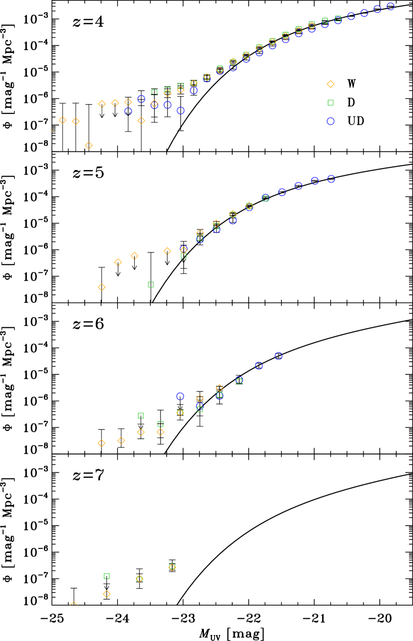
Figure 13: Rest-frame UV luminosity functions of dropouts at $z\sim 4$, $z\sim 5$, $z\sim 6$, and $z\sim 7$ derived for our dropout samples in the W (orange diamonds), D (green squares), and UD (blue circles) layers separately, where the quasar contamination correction is not taken into account. The symbols with a downward arrow denote the $1\sigma$ upper limits. The solid lines denote the best-fit Schechter functions shown in Figure 9.

References

- Abazajian et al. (2004) Abazajian, K., Adelman-McCarthy, J. K., Agüeros, M. A., et al. 2004, AJ, 128, 502
- Adelberger & Steidel (2000) Adelberger, K. L., & Steidel, C. C. 2000, ApJ, 544, 218
- Aihara et al. (2017a) Aihara, H., Armstrong, R., Bickerton, S., et al. 2017a, ArXiv e-prints, arXiv:1702.08449
- Aihara et al. (2017b) Aihara, H., Arimoto, N., Armstrong, R., et al. 2017b, ArXiv e-prints, arXiv:1704.05858
- Akiyama et al. (2017) Akiyama, M., He, W., Ikeda, H., et al. 2017, ArXiv e-prints, arXiv:1704.05996
- Atek et al. (2015) Atek, H., Richard, J., Jauzac, M., et al. 2015, ApJ, 814, 69
- Axelrod et al. (2010) Axelrod, T., Kantor, J., Lupton, R. H., & Pierfederici, F. 2010, in Proc. SPIE, Vol. 7740, Software and Cyberinfrastructure for Astronomy, 774015
- Bañados et al. (2016) Bañados, E., Venemans, B. P., Decarli, R., et al. 2016, ApJS, 227, 11
- Barone-Nugent et al. (2015) Barone-Nugent, R. L., Wyithe, J. S. B., Trenti, M., et al. 2015, MNRAS, 450, 1224
- Benson et al. (2003) Benson, A. J., Bower, R. G., Frenk, C. S., et al. 2003, ApJ, 599, 38
- Bian et al. (2013) Bian, F., Fan, X., Jiang, L., et al. 2013, ApJ, 774, 28
- Binney (1977) Binney, J. 1977, ApJ, 215, 483
- Binney (2004) —. 2004, MNRAS, 347, 1093
- Bosch et al. (2017) Bosch, J., Armstrong, R., Bickerton, S., et al. 2017, ArXiv e-prints, arXiv:1705.06766
- Bouwens et al. (2008) Bouwens, R. J., Illingworth, G. D., Franx, M., & Ford, H. 2008, ApJ, 686, 230
- Bouwens et al. (2017a) Bouwens, R. J., Illingworth, G. D., Oesch, P. A., et al. 2017a, ApJ, 843, 41
- Bouwens et al. (2017b) Bouwens, R. J., Oesch, P. A., Illingworth, G. D., Ellis, R. S., & Stefanon, M. 2017b, ApJ, 843, 129
- Bouwens et al. (2014) Bouwens, R. J., Illingworth, G. D., Oesch, P. A., et al. 2014, ApJ, 793, 115
- Bouwens et al. (2015) —. 2015, ApJ, 803, 34
- Bower et al. (2006) Bower, R. G., Benson, A. J., Malbon, R., et al. 2006, MNRAS, 370, 645
- Bowler et al. (2017) Bowler, R. A. A., Dunlop, J. S., McLure, R. J., & McLeod, D. J. 2017, MNRAS, 466, 3612
- Bowler et al. (2012) Bowler, R. A. A., Dunlop, J. S., McLure, R. J., et al. 2012, MNRAS, 426, 2772
- Bowler et al. (2015) —. 2015, MNRAS, 452, 1817
- Bruzual & Charlot (2003) Bruzual, G., & Charlot, S. 2003, MNRAS, 344, 1000
- Calzetti et al. (2000) Calzetti, D., Armus, L., Bohlin, R. C., et al. 2000, ApJ, 533, 682
- Capak et al. (2007) Capak, P., Aussel, H., Ajiki, M., et al. 2007, ApJS, 172, 99
- Castellano et al. (2010) Castellano, M., Fontana, A., Boutsia, K., et al. 2010, A&A, 511, A20
- Castellano et al. (2016) Castellano, M., Yue, B., Ferrara, A., et al. 2016, ApJ, 823, L40
- Coleman et al. (1980) Coleman, G. D., Wu, C.-C., & Weedman, D. W. 1980, ApJS, 43, 393
- Coupon et al. (2017) Coupon, J., Czakon, N., Bosch, J., et al. 2017, ArXiv e-prints, arXiv:1705.00622
- Croton et al. (2006) Croton, D. J., Springel, V., White, S. D. M., et al. 2006, MNRAS, 365, 11
- Curtis-Lake et al. (2012) Curtis-Lake, E., McLure, R. J., Pearce, H. J., et al. 2012, MNRAS, 422, 1425
- Curtis-Lake et al. (2016) Curtis-Lake, E., McLure, R. J., Dunlop, J. S., et al. 2016, MNRAS, 457, 440
- Dressler et al. (2011) Dressler, A., Bigelow, B., Hare, T., et al. 2011, PASP, 123, 288
- Eddington (1913) Eddington, A. S. 1913, MNRAS, 73, 359
- Ellis et al. (2013) Ellis, R. S., McLure, R. J., Dunlop, J. S., et al. 2013, ApJ, 763, L7
- Faber & Jackson (1976) Faber, S. M., & Jackson, R. E. 1976, ApJ, 204, 668
- Finkelstein et al. (2015) Finkelstein, S. L., Ryan, Jr., R. E., Papovich, C., et al. 2015, ApJ, 810, 71
- Finlator et al. (2017) Finlator, K., Prescott, M. K. M., Oppenheimer, B. D., et al. 2017, MNRAS, 464, 1633
- Furusawa et al. (2008) Furusawa, H., Kosugi, G., Akiyama, M., et al. 2008, ApJS, 176, 1
- Furusawa et al. (2017) Furusawa, H., et al. 2017, submitted to PASJ
- Gehrels (1986) Gehrels, N. 1986, ApJ, 303, 336
- Giallongo et al. (2015) Giallongo, E., Grazian, A., Fiore, F., et al. 2015, A&A, 578, A83
- Giavalisco (2002) Giavalisco, M. 2002, ARA&A, 40, 579
- Glikman et al. (2011) Glikman, E., Djorgovski, S. G., Stern, D., et al. 2011, ApJ, 728, L26
- Gnedin (2016) Gnedin, N. Y. 2016, ApJ, 825, L17
- Granato et al. (2004) Granato, G. L., De Zotti, G., Silva, L., Bressan, A., & Danese, L. 2004, ApJ, 600, 580
- Gunn & Stryker (1983) Gunn, J. E., & Stryker, L. L. 1983, ApJS, 52, 121
- Harikane et al. (2017) Harikane, Y., Ouchi, M., Ono, Y., et al. 2017, ArXiv e-prints, arXiv:1704.06535
- Hildebrandt et al. (2009) Hildebrandt, H., Pielorz, J., Erben, T., et al. 2009, A&A, 498, 725
- Hogg (1999) Hogg, D. W. 1999, ArXiv Astrophysics e-prints, astro-ph/9905116
- Hook et al. (2004) Hook, I. M., Jørgensen, I., Allington-Smith, J. R., et al. 2004, PASP, 116, 425
- Huang et al. (2017) Huang, S., Leauthaud, A., Murata, R., et al. 2017, ArXiv e-prints, arXiv:1705.01599
- Ikeda et al. (2012) Ikeda, H., Nagao, T., Matsuoka, K., et al. 2012, ApJ, 756, 160
- Ishigaki et al. (2017) Ishigaki, M., Kawamata, R., Ouchi, M., Oguri, M., & Shimasaku, K. 2017, ArXiv e-prints, arXiv:1702.04867
- Ishigaki et al. (2015) Ishigaki, M., Kawamata, R., Ouchi, M., et al. 2015, ApJ, 799, 12
- Ivezic et al. (2008) Ivezic, Z., Tyson, J. A., Abel, B., et al. 2008, ArXiv e-prints, arXiv:0805.2366
- Iwata et al. (2007) Iwata, I., Ohta, K., Tamura, N., et al. 2007, MNRAS, 376, 1557
- Jaacks et al. (2013) Jaacks, J., Thompson, R., & Nagamine, K. 2013, ApJ, 766, 94
- Jiang et al. (2016) Jiang, L., McGreer, I. D., Fan, X., et al. 2016, ApJ, 833, 222
- Jurić et al. (2015) Jurić, M., Kantor, J., Lim, K., et al. 2015, ArXiv e-prints, arXiv:1512.07914
- Kashikawa et al. (2002) Kashikawa, N., Aoki, K., Asai, R., et al. 2002, PASJ, 54, 819
- Kashikawa et al. (2006) Kashikawa, N., Shimasaku, K., Malkan, M. A., et al. 2006, ApJ, 648, 7
- Kashikawa et al. (2015) Kashikawa, N., Ishizaki, Y., Willott, C. J., et al. 2015, ApJ, 798, 28
- Kawamata et al. (2015) Kawamata, R., Ishigaki, M., Shimasaku, K., Oguri, M., & Ouchi, M. 2015, ApJ, 804, 103
- Kawamata et al. (2016) Kawamata, R., Oguri, M., Ishigaki, M., Shimasaku, K., & Ouchi, M. 2016, ApJ, 819, 114
- Kawanomoto et al. (2017) Kawanomoto, S., et al. 2017, to be submitted to PASJ
- Kelvin et al. (2014) Kelvin, L. S., Driver, S. P., Robotham, A. S. G., et al. 2014, MNRAS, 439, 1245
- Knapp et al. (2004) Knapp, G. R., Leggett, S. K., Fan, X., et al. 2004, AJ, 127, 3553
- Komiyama et al. (2017) Komiyama, Y., et al. 2017, submitted to PASJ
- Konno et al. (2017) Konno, A., Ouchi, M., Shibuya, T., et al. 2017, ArXiv e-prints, arXiv:1705.01222
- Kriek et al. (2015) Kriek, M., Shapley, A. E., Reddy, N. A., et al. 2015, ApJS, 218, 15
- Krumholz & Dekel (2012) Krumholz, M. R., & Dekel, A. 2012, ApJ, 753, 16
- Kuhlen et al. (2013) Kuhlen, M., Madau, P., & Krumholz, M. R. 2013, ApJ, 776, 34
- Le Fèvre et al. (2013) Le Fèvre, O., Cassata, P., Cucciati, O., et al. 2013, A&A, 559, A14
- Lilly et al. (2009) Lilly, S. J., Le Brun, V., Maier, C., et al. 2009, ApJS, 184, 218
- Liu et al. (2016) Liu, C., Mutch, S. J., Angel, P. W., et al. 2016, MNRAS, 462, 235
- Livermore et al. (2017) Livermore, R. C., Finkelstein, S. L., & Lotz, J. M. 2017, ApJ, 835, 113
- Loveday et al. (2012) Loveday, J., Norberg, P., Baldry, I. K., et al. 2012, MNRAS, 420, 1239
- Madau (1995) Madau, P. 1995, ApJ, 441, 18
- Magnier et al. (2013) Magnier, E. A., Schlafly, E., Finkbeiner, D., et al. 2013, ApJS, 205, 20
- Mallery et al. (2012) Mallery, R. P., Mobasher, B., Capak, P., et al. 2012, ApJ, 760, 128
- Martin et al. (2005) Martin, D. C., Seibert, M., Buat, V., et al. 2005, ApJ, 619, L59
- Mason et al. (2015) Mason, C. A., Treu, T., Schmidt, K. B., et al. 2015, ApJ, 805, 79
- Masters et al. (2012) Masters, D., Capak, P., Salvato, M., et al. 2012, ApJ, 755, 169
- Masters et al. (2017) Masters, D. C., Stern, D. K., Cohen, J. G., et al. 2017, ApJ, 841, 111
- Matsuoka et al. (2016) Matsuoka, Y., Onoue, M., Kashikawa, N., et al. 2016, ApJ, 828, 26
- Matsuoka et al. (2017) —. 2017, ArXiv e-prints, arXiv:1704.05854
- McGreer et al. (2013) McGreer, I. D., Jiang, L., Fan, X., et al. 2013, ApJ, 768, 105
- McLeod et al. (2016) McLeod, D. J., McLure, R. J., & Dunlop, J. S. 2016, MNRAS, 459, 3812
- McLure et al. (2009) McLure, R. J., Cirasuolo, M., Dunlop, J. S., Foucaud, S., & Almaini, O. 2009, MNRAS, 395, 2196
- McLure et al. (2013) McLure, R. J., Dunlop, J. S., Bowler, R. A. A., et al. 2013, MNRAS, 432, 2696
- Miyazaki et al. (2012) Miyazaki, S., Komiyama, Y., Nakaya, H., et al. 2012, in Proc. SPIE, Vol. 8446, Ground-based and Airborne Instrumentation for Astronomy IV, 84460Z
- Miyazaki et al. (2017) Miyazaki, S., et al. 2017, PASJ in press
- Momcheva et al. (2016) Momcheva, I. G., Brammer, G. B., van Dokkum, P. G., et al. 2016, ApJS, 225, 27
- Mosleh et al. (2012) Mosleh, M., Williams, R. J., Franx, M., et al. 2012, ApJ, 756, L12
- Muñoz & Loeb (2011) Muñoz, J. A., & Loeb, A. 2011, ApJ, 729, 99
- Murata et al. (2017) Murata, R., et al. 2017, to be submitted to PASJ
- Murayama et al. (2007) Murayama, T., Taniguchi, Y., Scoville, N. Z., et al. 2007, ApJS, 172, 523
- Niida et al. (2016) Niida, M., Nagao, T., Ikeda, H., et al. 2016, ApJ, 832, 208
- Ocvirk et al. (2016) Ocvirk, P., Gillet, N., Shapiro, P. R., et al. 2016, MNRAS, 463, 1462
- Oesch et al. (2010) Oesch, P. A., Bouwens, R. J., Carollo, C. M., et al. 2010, ApJ, 709, L21
- Oke & Gunn (1983) Oke, J. B., & Gunn, J. E. 1983, ApJ, 266, 713
- Ono et al. (2013) Ono, Y., Ouchi, M., Curtis-Lake, E., et al. 2013, ApJ, 777, 155
- O’Shea et al. (2015) O’Shea, B. W., Wise, J. H., Xu, H., & Norman, M. L. 2015, ApJ, 807, L12
- Ouchi et al. (2004) Ouchi, M., Shimasaku, K., Okamura, S., et al. 2004, ApJ, 611, 660
- Ouchi et al. (2008) Ouchi, M., Shimasaku, K., Akiyama, M., et al. 2008, ApJS, 176, 301
- Ouchi et al. (2009) Ouchi, M., Mobasher, B., Shimasaku, K., et al. 2009, ApJ, 706, 1136
- Ouchi et al. (2010) Ouchi, M., Shimasaku, K., Furusawa, H., et al. 2010, ApJ, 723, 869
- Ouchi et al. (2017) Ouchi, M., Harikane, Y., Shibuya, T., et al. 2017, ArXiv e-prints, arXiv:1704.07455
- Pâris et al. (2017) Pâris, I., Petitjean, P., Ross, N. P., et al. 2017, A&A, 597, A79
- Parsa et al. (2017) Parsa, S., Dunlop, J. S., & McLure, R. J. 2017, ArXiv e-prints, arXiv:1704.07750
- Ravindranath et al. (2006) Ravindranath, S., Giavalisco, M., Ferguson, H. C., et al. 2006, ApJ, 652, 963
- Reddy et al. (2008) Reddy, N. A., Steidel, C. C., Pettini, M., et al. 2008, ApJS, 175, 48
- Rees & Ostriker (1977) Rees, M. J., & Ostriker, J. P. 1977, MNRAS, 179, 541
- Ribeiro et al. (2016) Ribeiro, B., Le Fèvre, O., Tasca, L. A. M., et al. 2016, A&A, 593, A22
- Rowe et al. (2015) Rowe, B. T. P., Jarvis, M., Mandelbaum, R., et al. 2015, Astronomy and Computing, 10, 121
- Saito et al. (2008) Saito, T., Shimasaku, K., Okamura, S., et al. 2008, ApJ, 675, 1076
- Salpeter (1955) Salpeter, E. E. 1955, ApJ, 121, 161
- Sawicki & Thompson (2006) Sawicki, M., & Thompson, D. 2006, ApJ, 642, 653
- Scannapieco & Oh (2004) Scannapieco, E., & Oh, S. P. 2004, ApJ, 608, 62
- Schechter (1976) Schechter, P. 1976, ApJ, 203, 297
- Schenker et al. (2013) Schenker, M. A., Robertson, B. E., Ellis, R. S., et al. 2013, ApJ, 768, 196
- Schlafly et al. (2012) Schlafly, E. F., Finkbeiner, D. P., Jurić, M., et al. 2012, ApJ, 756, 158
- Schlegel et al. (1998) Schlegel, D. J., Finkbeiner, D. P., & Davis, M. 1998, ApJ, 500, 525
- Shibuya et al. (2015) Shibuya, T., Ouchi, M., & Harikane, Y. 2015, ApJS, 219, 15
- Shibuya et al. (2017a) Shibuya, T., Ouchi, M., Konno, A., et al. 2017a, ArXiv e-prints, arXiv:1704.08140
- Shibuya et al. (2017b) Shibuya, T., Ouchi, M., Harikane, Y., et al. 2017b, ArXiv e-prints, arXiv:1705.00733
- Shimasaku et al. (2005) Shimasaku, K., Ouchi, M., Furusawa, H., et al. 2005, PASJ, 57, 447
- Shimasaku et al. (2006) Shimasaku, K., Kashikawa, N., Doi, M., et al. 2006, PASJ, 58, 313
- Shioya et al. (2009) Shioya, Y., Taniguchi, Y., Sasaki, S. S., et al. 2009, ApJ, 696, 546
- Silk (1977) Silk, J. 1977, ApJ, 211, 638
- Stark (2016) Stark, D. P. 2016, ARA&A, 54, 761
- Stefanon et al. (2017) Stefanon, M., Labbé, I., Bouwens, R. J., et al. 2017, ArXiv e-prints, arXiv:1706.04613
- Steidel et al. (1999) Steidel, C. C., Adelberger, K. L., Giavalisco, M., Dickinson, M., & Pettini, M. 1999, ApJ, 519, 1
- Steidel et al. (1996) Steidel, C. C., Giavalisco, M., Pettini, M., Dickinson, M., & Adelberger, K. L. 1996, ApJ, 462, L17
- Takahashi et al. (2011) Takahashi, R., Oguri, M., Sato, M., & Hamana, T. 2011, ApJ, 742, 15
- Takata et al. (2017) Takata, T., et al. 2017, to be submitted to PASJ
- Tasca et al. (2017) Tasca, L. A. M., Le Fèvre, O., Ribeiro, B., et al. 2017, A&A, 600, A110
- Tonry et al. (2012) Tonry, J. L., Stubbs, C. W., Lykke, K. R., et al. 2012, ApJ, 750, 99
- Toshikawa et al. (2016) Toshikawa, J., Kashikawa, N., Overzier, R., et al. 2016, ApJ, 826, 114
- Toshikawa et al. (2017) Toshikawa, J., et al. 2017, PASJ in press
- Trenti & Stiavelli (2008) Trenti, M., & Stiavelli, M. 2008, ApJ, 676, 767
- van der Burg et al. (2010) van der Burg, R. F. J., Hildebrandt, H., & Erben, T. 2010, A&A, 523, A74
- Wang & Heckman (1996) Wang, B., & Heckman, T. M. 1996, ApJ, 457, 645
- Wang et al. (2016) Wang, F., Wu, X.-B., Fan, X., et al. 2016, ApJ, 819, 24
- Willott et al. (2010a) Willott, C. J., Albert, L., Arzoumanian, D., et al. 2010a, AJ, 140, 546
- Willott et al. (2010b) Willott, C. J., Delorme, P., Reylé, C., et al. 2010b, AJ, 139, 906
- Willott et al. (2013) Willott, C. J., McLure, R. J., Hibon, P., et al. 2013, AJ, 145, 4
- Wise et al. (2014) Wise, J. H., Demchenko, V. G., Halicek, M. T., et al. 2014, MNRAS, 442, 2560
- Wyithe et al. (2011) Wyithe, J. S. B., Yan, H., Windhorst, R. A., & Mao, S. 2011, Nature, 469, 181
- Yang et al. (2017) Yang, J., Fan, X., Wu, X.-B., et al. 2017, AJ, 153, 184
- Yoshida et al. (2006) Yoshida, M., Shimasaku, K., Kashikawa, N., et al. 2006, ApJ, 653, 988