On the Success Probability of the Box-Constrained Rounding and Babai Detectors

Abstract

In communications, one frequently needs to detect a parameter vector ${\hat{{\boldsymbol{x}}}}$ in a box from a linear model. The box-constrained rounding detector ${\boldsymbol{x}}^{\scriptscriptstyle\text{BR}}$ and Babai detector ${\boldsymbol{x}}^{\scriptscriptstyle\text{BB}}$ are often used to detect ${\hat{{\boldsymbol{x}}}}$ due to their high probability of correct detection, which is referred to as success probability, and their high efficiency of implimentation. It is generally believed that the success probability $P^{\scriptscriptstyle\text{BR}}$ of ${\boldsymbol{x}}^{\scriptscriptstyle\text{BR}}$ is not larger than the success probability $P^{\scriptscriptstyle\text{BB}}$ of ${\boldsymbol{x}}^{\scriptscriptstyle\text{BB}}$. In this paper, we first present formulas for $P^{\scriptscriptstyle\text{BR}}$ and $P^{\scriptscriptstyle\text{BB}}$ for two different situations: ${\hat{{\boldsymbol{x}}}}$ is deterministic and ${\hat{{\boldsymbol{x}}}}$ is uniformly distributed over the constraint box. Then, we give a simple example to show that $P^{\scriptscriptstyle\text{BR}}$ may be strictly larger than $P^{\scriptscriptstyle\text{BB}}$ if ${\hat{{\boldsymbol{x}}}}$ is deterministic, while we rigorously show that $P^{\scriptscriptstyle\text{BR}}\leq P^{\scriptscriptstyle\text{BB}}$ always holds if ${\hat{{\boldsymbol{x}}}}$ is uniformly distributed over the constraint box.

I Introduction

Suppose that we have the following box-constrained linear model:

$${\boldsymbol{y}}=\boldsymbol{A}{\hat{{\boldsymbol{x}}}}+\boldsymbol{v},\quad\boldsymbol{v}\sim\mathcal{N}(\boldsymbol{0},\sigma^{2}\boldsymbol{I}),$$ (1)

$${\hat{{\boldsymbol{x}}}}\in\mathcal{B}\equiv\{{\boldsymbol{x}}\in\mathbb{Z}^{n}:\boldsymbol{\ell}\leq{\boldsymbol{x}}\leq\boldsymbol{u},\;\boldsymbol{\ell},\boldsymbol{u}\in\mathbb{Z}^{n}\},$$ (2)

where ${\boldsymbol{y}}\in\mathbb{R}^{m}$ is an observation vector, $\boldsymbol{A}\in\mathbb{R}^{m\times n}$ is a deterministic full column rank model matrix, ${\hat{{\boldsymbol{x}}}}$ which can be deterministic or random is an unknown integer parameter vector in the box $\mathcal{B}$, $\boldsymbol{v}\in\mathbb{R}^{m}$ is a noise vector following the Gaussian distribution $\mathcal{N}(\boldsymbol{0},\sigma^{2}\boldsymbol{I})$ with given $\sigma$. This model arises from lots of applications including wireless communications, see e.g., [1].

Since $\boldsymbol{v}\sim\mathcal{N}(\boldsymbol{0},\sigma^{2}\boldsymbol{I})$, a commonly used method to detect ${\hat{{\boldsymbol{x}}}}$ is to solve the following box-constrained integer least squares (BILS) problem:

$$\min_{{\boldsymbol{x}}\in\mathcal{B}}\|{\boldsymbol{y}}-\boldsymbol{A}{\boldsymbol{x}}\|_{2}^{2},$$ (3)

whose solution is the maximum likelihood detector of ${\hat{{\boldsymbol{x}}}}$.

If ${\hat{{\boldsymbol{x}}}}\in{\mathbb{Z}}^{n}$ in (1) is not subject to any constraint, then (1) is called as an ordinary linear model. In this case, to get the maximum likelihood estimator of ${\hat{{\boldsymbol{x}}}}$, we solve the following ordinary integer least squares (OILS) problem:

$$\min_{{\boldsymbol{x}}\in\mathbb{Z}^{n}}\|{\boldsymbol{y}}-\boldsymbol{A}{\boldsymbol{x}}\|_{2}^{2}.$$ (4)

In communications, one of the widely used methods for solving (3) and (4) is sphere decoding. Although some column reordering strategies, such as V-BLAST [2], SQRD [3], and those proposed in [4] which use not only the information of $\boldsymbol{A}$, but also the information of ${\boldsymbol{y}}$ and $\mathcal{B}$, can usually reduce the computational cost of solving (3) by sphere decoding, solving (3) is still time-consuming especially when $\boldsymbol{A}$ is ill conditioned, $\sigma$ or $n$ is large [5]. Moreover, it has been shown in [6] that (4) is an NP-hard problem. Therefore, in practical applications, especially for some real-time applications, a suboptimal detector, which can be obtained efficiently, is often used to detect ${\hat{{\boldsymbol{x}}}}$ instead of solving (3) or (4) to get the optimal detector.

For the OILS problem, the ordinary rounding detector ${\boldsymbol{x}}^{\scriptscriptstyle\text{OR}}$ and the Babai detector ${\boldsymbol{x}}^{\scriptscriptstyle\text{OB}}$, which are respectively obtained by the Babai rounding off and nearest plane algorithms [7], are often used suboptimal detectors for ${\hat{{\boldsymbol{x}}}}$. By taking the box constraint (2) into account, one can easily modify the algorithms for ${\boldsymbol{x}}^{\scriptscriptstyle\text{OR}}$ and ${\boldsymbol{x}}^{\scriptscriptstyle\text{OB}}$ to get box-constrained rounding detectors ${\boldsymbol{x}}^{\scriptscriptstyle\text{BR}}$ and box-constrained Babai detectors ${\boldsymbol{x}}^{\scriptscriptstyle\text{BB}}$ for ${\hat{{\boldsymbol{x}}}}$ satisfying both (1) and (2). Rounding and Babai detectors are respectively the outputs of zero-forcing and successive interference cancellation decoders which are widely used suboptimal detection algorithms in communications.

To characterize how good a detector is, we use its success probability, i.e., the probability of the detector being equal to ${\hat{{\boldsymbol{x}}}}$, see e.g., [8, 9].

For the estimation of ${\hat{{\boldsymbol{x}}}}$ in the ordinary linear model (1), the formulas of the success probability $P^{\scriptscriptstyle\text{OR}}$ of the rounding detector ${\boldsymbol{x}}^{\scriptscriptstyle\text{OR}}$ and the success probability $P^{\scriptscriptstyle\text{OB}}$ of the Babai detector ${\boldsymbol{x}}^{\scriptscriptstyle\text{OB}}$ have been given in [10] and [8], respectively. Equivalent formulas of $P^{\scriptscriptstyle\text{OR}}$ and $P^{\scriptscriptstyle\text{OB}}$ were given earlier in [11], which considers the OILS problem in different formats in the application of GPS. It is shown in [11] that $P^{\scriptscriptstyle\text{OR}}\leq P^{\scriptscriptstyle\text{OB}}$.

For the detection of ${\hat{{\boldsymbol{x}}}}$ satisfying both (1) and (2), it is also generally believed that the success probability $P^{\scriptscriptstyle\text{BR}}$ of the rounding detector ${\boldsymbol{x}}^{\scriptscriptstyle\text{BR}}$ is not larger than the success probability $P^{\scriptscriptstyle\text{BB}}$ of the Babai detector ${\boldsymbol{x}}^{\scriptscriptstyle\text{BB}}$.

In this paper, we develop formulas for the success probability $P_{\scriptscriptstyle\text{D}}^{\scriptscriptstyle\text{BR}}$ and $P_{\scriptscriptstyle\text{R}}^{\scriptscriptstyle\text{BR}}$ of ${\boldsymbol{x}}^{\scriptscriptstyle\text{BR}}$ which respectively corresponding to the case that ${\hat{{\boldsymbol{x}}}}$ is a deterministic parameter vector and ${\hat{{\boldsymbol{x}}}}$ is uniformly distributed over $\mathcal{B}$. We also give a formula for the success probability $P_{\scriptscriptstyle\text{D}}^{\scriptscriptstyle\text{BB}}$ of the box-constrained Babai detector ${\boldsymbol{x}}^{\scriptscriptstyle\text{BB}}$ for the case that ${\hat{{\boldsymbol{x}}}}$ is deterministic. Note that the success probability $P_{\scriptscriptstyle\text{R}}^{\scriptscriptstyle\text{BB}}$ of ${\boldsymbol{x}}^{\scriptscriptstyle\text{BB}}$ for the case that ${\hat{{\boldsymbol{x}}}}$ is uniformly distributed over $\mathcal{B}$ has been given in [9]. We would like to point out that the assumption that ${\hat{{\boldsymbol{x}}}}$ follows the uniformly distribution is often made for MIMO applications, see, e.g., [5]. For the deterministic case, we give a simple example to show that $P_{\scriptscriptstyle\text{D}}^{\scriptscriptstyle\text{BR}}>P_{\scriptscriptstyle\text{D}}^{\scriptscriptstyle\text{BB}}$, contrary to what we have suspected. For the uniform random case, however, we rigorously show that the common belief is indeed true, i.e., $P_{\scriptscriptstyle\text{R}}^{\scriptscriptstyle\text{BR}}\leq P_{\scriptscriptstyle\text{R}}^{\scriptscriptstyle\text{BB}}$.

The rest of the paper is organized as follows. In Section II, we present formulas for $P_{\scriptscriptstyle\text{D}}^{\scriptscriptstyle\text{BR}}$, $P_{\scriptscriptstyle\text{R}}^{\scriptscriptstyle\text{BR}}$, $P_{\scriptscriptstyle\text{D}}^{\scriptscriptstyle\text{BB}}$ and $P_{\scriptscriptstyle\text{R}}^{\scriptscriptstyle\text{BB}}$. In Section III, we study the relationship between $P_{\scriptscriptstyle\text{D}}^{\scriptscriptstyle\text{BR}}$ and $P_{\scriptscriptstyle\text{D}}^{\scriptscriptstyle\text{BB}}$, and rigorously show that $P_{\scriptscriptstyle\text{R}}^{\scriptscriptstyle\text{BR}}\leq P_{\scriptscriptstyle\text{R}}^{\scriptscriptstyle\text{BB}}$. In Section IV, we do simulation tests to illustrate our main results. Finally we summarize this paper in Section V.

Notation. Throughout this paper, for ${\boldsymbol{x}}\in\mathbb{R}^{n}$, we use $\lfloor{\boldsymbol{x}}\rceil$ to denote its nearest integer vector, i.e., each entry of ${\boldsymbol{x}}$ is rounded to its nearest integer (if there is a tie, the one with smaller magnitude is chosen). For a vector ${\boldsymbol{x}}$, ${\boldsymbol{x}}_{i:j}$ denotes the subvector of ${\boldsymbol{x}}$ formed by entries $i,i+1,\ldots,j$. For a matrix $\boldsymbol{A}$, $\boldsymbol{A}_{i:j,i:j}$ denotes the submatrix of $\boldsymbol{A}$ formed by rows and columns $i,i+1,\ldots,j$.

II Success probability of box-constrained rounding and Babai detectors

In this section, we derive formulas for $P_{\scriptscriptstyle\text{D}}^{\scriptscriptstyle\text{BR}}$, $P_{\scriptscriptstyle\text{R}}^{\scriptscriptstyle\text{BR}}$ and $P_{\scriptscriptstyle\text{D}}^{\scriptscriptstyle\text{BB}}$. Note that the formula for $P_{\scriptscriptstyle\text{R}}^{\scriptscriptstyle\text{BB}}$ has been derived in [9, Th.1].

Let $\boldsymbol{A}$ in (1) have the QR factorization

$$\boldsymbol{A}=[\boldsymbol{Q}_{1},\boldsymbol{Q}_{2}]\begin{bmatrix}\boldsymbol{R}\\ {\boldsymbol{0}}\end{bmatrix},$$ (5)

where $[\underset{n}{\boldsymbol{Q}_{1}},\underset{m-n}{\boldsymbol{Q}_{2}}]\in{\mathbb{R}}^{m\times m}$ is orthogonal and $\boldsymbol{R}\in{\mathbb{R}}^{n\times n}$ is upper triangular. Without loss of generality, we assume that $r_{ii}>0$ for $i=1,\ldots,n$ throughout the paper.

Define ${\tilde{{\boldsymbol{y}}}}=\boldsymbol{Q}_{1}^{T}{\boldsymbol{y}}$ and $\tilde{\boldsymbol{v}}=\boldsymbol{Q}_{1}^{T}\boldsymbol{v}$. Then, left multiplying both sides of (1) with $\boldsymbol{Q}_{1}^{T}$ yields

$${\tilde{{\boldsymbol{y}}}}=\boldsymbol{R}{\hat{{\boldsymbol{x}}}}+\tilde{\boldsymbol{v}},\quad\tilde{\boldsymbol{v}}\sim\mathcal{N}({\boldsymbol{0}},\sigma^{2}\boldsymbol{I}).$$ (6)

Let $\boldsymbol{d}=\boldsymbol{R}^{-1}{\tilde{{\boldsymbol{y}}}}$, then the box-constrained rounding detector ${\boldsymbol{x}}^{\scriptscriptstyle\text{BR}}$ and box-constrained Babai detector ${\boldsymbol{x}}^{\scriptscriptstyle\text{BB}}$ of (6) can be respectively computed as follows:

$$\begin{split}x_{i}^{\scriptscriptstyle\text{BR}}=\begin{cases}\ell_{i},\quad\mbox{ if }\lfloor d_{i}\rceil\leq\ell_{i},\\ \lfloor d_{i}\rceil,\mbox{ if }\ell_{i}<\lfloor d_{i}\rceil<u_{i},\quad i=1,\ldots,n\\ u_{i},\quad\mbox{ if }\lfloor d_{i}\rceil\geq u_{i},\end{cases}\end{split}$$ (7)

and

$$\begin{split}&c_{i}=({\tilde{y}}_{i}-\sum_{j=i+1}^{n}r_{ij}x_{j}^{\scriptscriptstyle\text{BB}})/r_{ii},\\ &x_{i}^{\scriptscriptstyle\text{BB}}=\begin{cases}\ell_{i},&\mbox{ if }\ \lfloor c_{i}\rceil\leq\ell_{i},\\ \lfloor c_{i}\rceil,&\mbox{ if }\ \ell_{i}<\lfloor c_{i}\rceil<u_{i},\,\;i=n,\ldots,1.\\ u_{i},&\mbox{ if }\ \lfloor c_{i}\rceil\geq u_{i},\end{cases}\end{split}$$ (8)

where $\sum_{j=n+1}^{n}r_{nj}x_{j}^{\scriptscriptstyle\text{BB}}=0$.

II-A Success probability of the box-constrained rounding detector

In this subsection, we develop formulas for $P_{\scriptscriptstyle\text{D}}^{\scriptscriptstyle\text{BR}}$ and $P_{\scriptscriptstyle\text{R}}^{\scriptscriptstyle\text{BR}}$. Since $P_{\scriptscriptstyle\text{D}}^{\scriptscriptstyle\text{BR}}$ depends on the position of ${\hat{{\boldsymbol{x}}}}$ in the box $\mathcal{B}$, we also give a lower bound on $P_{\scriptscriptstyle\text{D}}^{\scriptscriptstyle\text{BR}}$.

Theorem 1

Let ${\hat{{\boldsymbol{x}}}}$ in (1) be a deterministic vector, then

$$P_{\scriptscriptstyle\text{D}}^{\scriptscriptstyle\text{BR}}=\frac{\det(\boldsymbol{R})}{(2\pi\sigma^{2})^{n/2}}\int_{I_{n}}\cdots\int_{I_{1}}\exp\left(-\frac{\|\boldsymbol{R}\boldsymbol{\xi}\|^{2}_{2}}{2\sigma^{2}}\right)d\xi_{1}\cdots d\xi_{n},$$ (9)

where

$$I_{i}=\begin{cases}(-\infty,\frac{1}{2}],\quad\mbox{ if }{\hat{x}}_{i}=\ell_{i}\quad\\ [-\frac{1}{2},\frac{1}{2}],\quad\,\;\mbox{ if }\ell_{i}<{\hat{x}}_{i}<u_{i}.\\ [-\frac{1}{2},\infty),\quad\mbox{ if }{\hat{x}}_{i}=u_{i}\end{cases}$$ (10)

Proof. Since ${\hat{{\boldsymbol{x}}}}$ is deterministic and $\tilde{\boldsymbol{v}}\sim\mathcal{N}({\boldsymbol{0}},\sigma^{2}\boldsymbol{I})$, by (6), we have

$$\boldsymbol{d}-{\hat{{\boldsymbol{x}}}}=\boldsymbol{R}^{-1}{\tilde{{\boldsymbol{y}}}}-{\hat{{\boldsymbol{x}}}}=\boldsymbol{R}^{-1}\tilde{\boldsymbol{v}}\sim\mathcal{N}({\boldsymbol{0}},\sigma^{2}(\boldsymbol{R}^{T}\boldsymbol{R})^{-1}).$$

By the definition of $\lfloor{\boldsymbol{x}}\rceil$, (7) and (10),

$${\boldsymbol{x}}^{\scriptscriptstyle\text{BR}}={\hat{{\boldsymbol{x}}}}\Leftrightarrow d_{i}-\hat{x}_{i}\in I_{i},\ \ i=1,\ldots,n.$$

Therefore, (9) holds.   $\Box$

From (9), $P_{\scriptscriptstyle\text{D}}^{\scriptscriptstyle\text{BR}}$ depends on the positions of the entries of ${\hat{{\boldsymbol{x}}}}$, thus we also write $P_{\scriptscriptstyle\text{D}}^{\scriptscriptstyle\text{BR}}$ as $P_{\scriptscriptstyle\text{D}}^{\scriptscriptstyle\text{BR}}({\hat{{\boldsymbol{x}}}})$.

According to (9), to compute $P_{\scriptscriptstyle\text{D}}^{\scriptscriptstyle\text{BR}}$, we need to know the positions of $\hat{x}_{i}$ on $[\ell_{i},u_{i}]$ for $i=1,\ldots,n$. In practice this information is unknown. However, it is easy to observe from (9) that $P_{\scriptscriptstyle\text{D}}^{\scriptscriptstyle\text{BR}}$ has a lower bound which does not rely on the position of ${\hat{{\boldsymbol{x}}}}$ in the box.

Corollary 1

Let ${\hat{{\boldsymbol{x}}}}$ in (1) be a deterministic vector, then

$$\ P_{\scriptscriptstyle\text{D}}^{\scriptscriptstyle\text{BR}}\geq \frac{\det(\boldsymbol{R})}{(2\pi\sigma^{2})^{n/2}}$$

$$\times\int_{-1/2}^{1/2}\cdots\int_{-1/2}^{1/2}\exp\left(-\frac{\|\boldsymbol{R}\boldsymbol{\xi}\|^{2}_{2}}{2\sigma^{2}}\right)d\xi_{1}\cdots d\xi_{n},$$

where the lower bound is reached if and only if $\ell_{i}<{\hat{x}}_{i}<u_{i}$ for $i=1,\ldots,n$.

The lower bound is actually the success probability of the ordinary rounding detector, i.e., $P^{\scriptscriptstyle\text{OR}}$, see [10, Th. 1]. It is easy to understand this. In fact, the ordinary case can be regarded as a special situation of the box-constrained case: $\ell_{i}=-\infty$ and $u_{i}=\infty$, thus, $\ell_{i}<{\hat{x}}_{i}<u_{i}$ for $i=1,\ldots,n$. Then, the lower bound is reached and it is just $P^{\scriptscriptstyle\text{OR}}$.

The following theorem gives a formula for $P_{\scriptscriptstyle\text{R}}^{\scriptscriptstyle\text{BR}}$.

Theorem 2

Suppose that ${\hat{{\boldsymbol{x}}}}$ in (1) is uniformly distributed over $\mathcal{B}$, and ${\hat{{\boldsymbol{x}}}}$ and $\boldsymbol{v}$ are independent, then

$$P_{\scriptscriptstyle\text{R}}^{\scriptscriptstyle\text{BR}}=\frac{1}{\prod_{i=1}^{n}(u_{i}-\ell_{i}+1)}\sum_{\forall\bar{{\boldsymbol{x}}}\in\mathcal{B}}P_{\scriptscriptstyle\text{D}}^{\scriptscriptstyle\text{BR}}(\bar{{\boldsymbol{x}}}).$$ (11)

Proof. Notice that

$$\Pr({\boldsymbol{x}}^{\scriptscriptstyle\text{BR}}={\hat{{\boldsymbol{x}}}}) =\sum_{\forall\bar{{\boldsymbol{x}}}\in\mathcal{B}}\Pr({\boldsymbol{x}}^{\scriptscriptstyle\text{BR}}={\hat{{\boldsymbol{x}}}}|{\hat{{\boldsymbol{x}}}}={\bar{{\boldsymbol{x}}}})\Pr({\hat{{\boldsymbol{x}}}}={\bar{{\boldsymbol{x}}}})$$

$$=\sum_{\forall\bar{{\boldsymbol{x}}}\in\mathcal{B}}\Pr({\boldsymbol{x}}^{\scriptscriptstyle\text{BR}}={\bar{{\boldsymbol{x}}}})\Pr({\hat{{\boldsymbol{x}}}}={\bar{{\boldsymbol{x}}}}).$$

Since ${\hat{{\boldsymbol{x}}}}$ is uniformly distributed over $\mathcal{B}$, for each $\bar{{\boldsymbol{x}}}\in\mathcal{B}$,

$$\Pr({\hat{{\boldsymbol{x}}}}=\bar{{\boldsymbol{x}}})=\frac{1}{\prod_{i=1}^{n}(u_{i}-\ell_{i}+1)}.$$

Therefore, (11) holds.   $\Box$

Note that $P_{\scriptscriptstyle\text{R}}^{\scriptscriptstyle\text{BR}}$ can be computed, although the computational cost may be high as the number of integer points in ${\cal B}$ can be large.

II-B Success probability of the box-constrained Babai detector

In this subsection, we give formulas for $P_{\scriptscriptstyle\text{D}}^{\scriptscriptstyle\text{BB}}$ and $P_{\scriptscriptstyle\text{R}}^{\scriptscriptstyle\text{BB}}$. Since $P_{\scriptscriptstyle\text{D}}^{\scriptscriptstyle\text{BB}}$ depends on the position of ${\hat{{\boldsymbol{x}}}}$ in the box $\mathcal{B}$, we also give a lower bound on $P_{\scriptscriptstyle\text{D}}^{\scriptscriptstyle\text{BB}}$.

We first consider the deterministic situation.

Theorem 3

Let ${\hat{{\boldsymbol{x}}}}$ in (1) be a deterministic vector, then

$$P_{\scriptscriptstyle\text{D}}^{\scriptscriptstyle\text{BB}}=\prod_{i=1}^{n}\omega_{i}(r_{ii}),$$ (12)

where

$$\omega_{i}(r_{ii})=\begin{cases}\frac{1}{2}\big{[}1+\phi_{\sigma}(r_{ii})\big{]},&\mbox{ if }\ {\hat{x}}_{i}=\ell_{i}\mbox{ or }{\hat{x}}_{i}=u_{i}\\ \phi_{\sigma}(r_{ii}),&\mbox{ if }\ \ell_{i}<{\hat{x}}_{i}<u_{i}\end{cases}$$ (13)

with

$$\phi_{\sigma}(\zeta) :=\frac{2}{\sqrt{2\pi}}\int_{0}^{\frac{\zeta}{2\sigma}}\exp\big{(}-\frac{1}{2}t^{2}\big{)}dt$$

$$=\frac{\zeta}{\sqrt{2\pi}\sigma}\int_{-\frac{1}{2}}^{\frac{1}{2}}\exp\big{(}\!-\frac{\zeta^{2}t^{2}}{2\sigma^{2}}\big{)}dt.$$ (14)

Proof. From (6), for $i=n,\ldots,1$,

$${\tilde{y}}_{i}=r_{ii}{\hat{x}}_{i}+\sum_{j=i+1}^{n}r_{ij}{\hat{x}}_{j}+{\tilde{v}}_{i}.$$

Then, using (8), we obtain

$$c_{i}={\hat{x}}_{i}+\sum_{j=i+1}^{n}\frac{r_{ij}}{r_{ii}}({\hat{x}}_{j}-x_{j}^{\scriptscriptstyle\text{BB}})+\frac{{\tilde{v}}_{i}}{r_{ii}}.$$ (15)

Therefore, if $x_{j}^{\scriptscriptstyle\text{BB}}={\hat{x}}_{j}$ for $j=i+1,\ldots,n$, then

$$c_{i}\sim\mathcal{N}({\hat{x}}_{i},\sigma^{2}/r_{ii}^{2}).$$

To simplify notation, denote events

$$E_{i}=(x_{i}^{\scriptscriptstyle\text{BB}}={\hat{x}}_{i},\ldots,x_{n}^{\scriptscriptstyle\text{BB}}={\hat{x}}_{n}),\quad i=1,\ldots,n.$$

Then by the chain rule of conditional probabilities,

$$P_{\scriptscriptstyle\text{D}}^{\scriptscriptstyle\text{BB}}=\Pr(E_{1})=\prod_{i=1}^{n}\Pr(x_{i}^{\scriptscriptstyle\text{BB}}={\hat{x}}_{i}|E_{i+1}),$$ (16)

where $E_{n+1}$ is the sample space $\Omega$.

Now we consider $\Pr(x_{i}^{\scriptscriptstyle\text{BB}}={\hat{x}}_{i}|E_{i+1})$ for three different cases.

Case 1: ${\hat{x}}_{i}=\ell_{i}$. In this case, by (8),

$$\Pr(x_{i}^{\scriptscriptstyle\text{BB}}={\hat{x}}_{i}\,|\,E_{i+1})$$

$$= \Pr(c_{i}\leq\ell_{i}+1/2\,|\,E_{i+1})$$

$$= \frac{1}{\sqrt{2\pi(\frac{\sigma}{r_{ii}})^{2}}}\int_{-\infty}^{\ell_{i}+\frac{1}{2}}\exp\Big{(}-\frac{(t-\ell_{i})^{2}}{2(\frac{\sigma}{r_{ii}})^{2}}\Big{)}dt$$

$$= \frac{1}{\sqrt{2\pi}}\int_{-\infty}^{\frac{r_{ii}}{2\sigma}}\exp\big{(}-\frac{t^{2}}{2}\big{)}dt=\frac{1}{2}[1+\phi_{\sigma}(r_{ii})].$$

Case 2: $\ell_{i}<{\hat{x}}_{i}<u_{i}$. In this case, by (8),

$$\Pr(x_{i}^{\scriptscriptstyle\text{BB}}={\hat{x}}_{i}\,|\,E_{i+1})$$

$$= \Pr({\hat{x}}_{i}-1/2\leq c_{i}\leq{\hat{x}}_{i}+1/2\,|\,E_{i+1})$$

$$= \frac{1}{\sqrt{2\pi(\frac{\sigma}{r_{ii}})^{2}}}\int^{{\hat{x}}_{i}+\frac{1}{2}}_{{\hat{x}}_{i}-\frac{1}{2}}\exp\Big{(}-\frac{(t-{\hat{x}}_{i})^{2}}{2(\frac{\sigma}{r_{ii}})^{2}}\Big{)}dt=\phi_{\sigma}(r_{ii}).$$

Case 3: ${\hat{x}}_{i}=u_{i}$. In this case, by (8),

$$\Pr(x_{i}^{\scriptscriptstyle\text{BB}}={\hat{x}}_{i}\,|\,E_{i+1})$$

$$= \Pr(u_{i}-1/2\leq c_{i}\,|\,E_{i+1})$$

$$= \frac{1}{\sqrt{2\pi(\frac{\sigma}{r_{ii}})^{2}}}\int_{u_{i}-\frac{1}{2}}^{\infty}\exp\Big{(}-\frac{(t-u_{i})^{2}}{2(\frac{\sigma}{r_{ii}})^{2}}\Big{)}dt$$

$$= \frac{1}{2}[1+\phi_{\sigma}(r_{ii})].$$

Therefore, from (16), this theorem holds.   $\Box$

The formula (12) was originally given in the MSc thesis [12], supervised by the second author of this paper. The proof given here is easier to follow than that given in [12]. Note that the main idea of its proof is similar to that of [9, Th. 1].

From Theorem 3, similarly to $P_{\scriptscriptstyle\text{D}}^{\scriptscriptstyle\text{BR}}$, to compute $P_{\scriptscriptstyle\text{D}}^{\scriptscriptstyle\text{BB}}$, we need to know the locations of $\hat{x}_{i}$ in the box $\mathcal{B}$. But, these information is usually unknown in practice. However, by (12) and (13), the following corollary which gives a lower bound and an upper bound on $P_{\scriptscriptstyle\text{D}}^{\scriptscriptstyle\text{BB}}$, that do not need priori information on ${\hat{{\boldsymbol{x}}}}$, clearly holds.

Corollary 2

Let ${\hat{{\boldsymbol{x}}}}$ in (1) be a deterministic vector, then

$$\prod_{i=1}^{n}\phi_{\sigma}(r_{ii})\leq P_{\scriptscriptstyle\text{D}}^{\scriptscriptstyle\text{BB}}\leq\frac{1}{2^{n}}\prod_{i=1}^{n}(1+\phi_{\sigma}(r_{ii})),$$ (17)

where the lower bound is reached if and only if $\ell_{i}<{\hat{x}}_{i}<u_{i}$ for $i=1,\ldots,n$, and the upper bound is reached if and only if ${\hat{x}}_{i}=\ell_{i}$ or ${\hat{x}}_{i}=u_{i}$ for $i=1,\ldots,n$.

The lower bound given in the corollary is actually the success probability of the ordinary Babai detector, see [8, eq. (11)].

For the random situation, we have the following theorem for computing $P_{\scriptscriptstyle\text{R}}^{\scriptscriptstyle\text{BB}}$, see [9, Th. 1].

Theorem 4

Suppose that ${\hat{{\boldsymbol{x}}}}$ in (1) is uniformly distributed over $\mathcal{B}$, and ${\hat{{\boldsymbol{x}}}}$ and $\tilde{\boldsymbol{v}}$ are independent, then

$$P_{\scriptscriptstyle\text{R}}^{\scriptscriptstyle\text{BB}}=\prod_{i=1}^{n}\Big{[}\frac{1}{u_{i}-\ell_{i}+1}+\frac{u_{i}-\ell_{i}}{u_{i}-\ell_{i}+1}\phi_{\sigma}(r_{ii})\Big{]},$$ (18)

where $\phi_{\sigma}(\zeta)$ is defined in (3).

III Relationship between $P^{\scriptscriptstyle\text{BR}}$ and $P^{\scriptscriptstyle\text{BB}}$

It has been showed in [11, eq. (20)] that the success probability of the ordinary rounding detector cannot be larger than that of the ordinary Babai detector. For the box-constrained case, in this section, we will show that the conclusion does not hold any more when the parameter vector is deterministic while it still holds when the parameter vector is uniformly distributed.

Simulations show that, in general, $P_{\scriptscriptstyle\text{D}}^{\scriptscriptstyle\text{BR}}\leq P_{\scriptscriptstyle\text{D}}^{\scriptscriptstyle\text{BB}}$. However, the following example shows that for the deterministic case it is possible that $P_{\scriptscriptstyle\text{D}}^{\scriptscriptstyle\text{BR}}>P_{\scriptscriptstyle\text{D}}^{\scriptscriptstyle\text{BB}}$.

Example 1

Let $\sigma=1$, $\boldsymbol{R}=\begin{bmatrix}2&-1\\ 0&1\end{bmatrix}$, ${\hat{x}}_{1}=\ell_{1}$ and ${\hat{x}}_{2}=\ell_{2}$. Then, by Theorems and 1 and 3, we have

$$P_{\scriptscriptstyle\text{D}}^{\scriptscriptstyle\text{BB}}=\frac{1}{4}(1+\phi_{1}(1))(1+\phi_{1}(2))=0.5818$$

and

$$P_{\scriptscriptstyle\text{D}}^{\scriptscriptstyle\text{BR}}=\frac{2}{2\pi}\int_{-\infty}^{1/2}\int_{-\infty}^{1/2}\exp(-\frac{1}{2}\|\boldsymbol{R}\boldsymbol{\xi}\|^{2}_{2})d\xi_{2}d\xi_{1}=0.6192.$$

Thus, $P_{\scriptscriptstyle\text{D}}^{\scriptscriptstyle\text{BR}}>P_{\scriptscriptstyle\text{D}}^{\scriptscriptstyle\text{BB}}$.

However, if ${\hat{{\boldsymbol{x}}}}$ is uniformly distributed over $\mathcal{B}$, then $P_{\scriptscriptstyle\text{D}}^{\scriptscriptstyle\text{BR}}<P_{\scriptscriptstyle\text{D}}^{\scriptscriptstyle\text{BB}}$. To prove this, we introduce a lemma.

Lemma 1

Suppose that $a>0$ and $s_{2},\ldots,s_{n}$ are intervals, then for any $\sigma>0$,

$$\int_{s_{n}}\cdots\int_{s_{2}}\int_{-a}^{a}\exp\left(-\frac{\|\boldsymbol{R}\boldsymbol{\xi}\|^{2}}{2\sigma^{2}}\right)d\xi_{1}\cdots d\xi_{n}$$

$$\leq \int_{-a}^{a}\exp\left(-\frac{r_{11}^{2}t^{2}}{2\sigma^{2}}\right)dt$$

$$\times\int_{s_{n}}\cdots\int_{s_{2}}\exp\left(-\frac{\|\boldsymbol{R}_{2:n,2:n}\boldsymbol{\xi}_{2:n}\|^{2}}{2\sigma^{2}}\right)d\xi_{2}\cdots d\xi_{n}.$$ (19)

Proof. We prove (1) by changing variables in the integral.

Let

$$\boldsymbol{T}=\begin{bmatrix}1&-\frac{1}{r_{11}}\boldsymbol{R}_{1,2:n}\\ {\boldsymbol{0}}&\boldsymbol{I}_{n-1}\end{bmatrix}.$$

Then

$$\boldsymbol{R}\boldsymbol{T}=\begin{bmatrix}r_{11}&0\\ {\boldsymbol{0}}&\boldsymbol{R}_{2:n,2:n}\end{bmatrix}.$$

Define $\boldsymbol{\xi}=\boldsymbol{T}\boldsymbol{\eta}$, then with

$$s_{1}:=\big{\{}\eta_{1}|-a\leq\eta_{1}-\sum_{j=2}^{n}\frac{r_{1j}}{r_{11}}\eta_{j}\leq a,\eta_{2}\in s_{2},\ldots,\eta_{n}\in s_{n}\big{\}}.$$

we have

$$\int_{s_{n}}\cdots\int_{s_{2}}\int_{-a}^{a}\exp\left(-\frac{\|\boldsymbol{R}\boldsymbol{\xi}\|^{2}}{2\sigma^{2}}\right)d\xi_{1}\cdots d\xi_{n}$$

$$= \int_{s_{n}}\cdots\int_{s_{1}}\exp\left(-\frac{r_{11}^{2}\eta^{2}_{1}+\|\boldsymbol{R}_{2:n,2:n}\boldsymbol{\eta}_{2:n}\|^{2}}{2\sigma^{2}}\right)d\eta_{1}\cdots d\eta_{n}$$

$$= \int_{s_{n}}\cdots\int_{s_{2}}\left(\int_{s_{1}}\exp\left(-\frac{r_{11}^{2}\eta^{2}_{1}}{2\sigma^{2}}\right)d\eta_{1}\right)$$

$$\times\exp\left(-\frac{\|\boldsymbol{R}_{2:n,2:n}\boldsymbol{\eta}_{2:n}\|^{2}}{2\sigma^{2}}\right)d\eta_{2}\cdots d\eta_{n}.$$

According to [9, eq. (68)], we have

$$\int_{s_{1}}\exp\left(-\frac{r_{11}^{2}\eta^{2}_{1}}{2\sigma^{2}}\right)d\eta_{1}\leq\int_{-a}^{a}\exp\left(-\frac{r_{11}^{2}t^{2}}{2\sigma^{2}}\right)dt.$$ (20)

Thus, (1) holds. Note that (20) can be easily observed from the graph of the density function of the normally distributed random variable with 0 mean. $\Box$

Here we make a remark. It is easy to see from the lemma that if $a_{i}>0$ for $i=1,\ldots,n$, then

$$\int_{-a_{n}}^{a_{n}}\cdots\int_{-a_{1}}^{a_{1}}\exp\left(-\frac{\|\boldsymbol{R}\boldsymbol{\xi}\|^{2}_{2}}{2\sigma^{2}}\right)d\xi_{1}\cdots d\xi_{n}$$

$$\leq \prod_{i=1}^{n}\int_{-a_{i}}^{a_{i}}\exp\left(-\frac{r_{ii}^{2}t^{2}}{2\sigma^{2}}\right)dt.$$

If $a_{i}=1/2$ for $i=1,\ldots,n$, the above inequality leads to [11, eq. (20)], which shows that the success probability of ordinary rounding detectors cannot be larger than the success probability of ordinary Babai detectors, but our proof is much simpler.

The following theorem characterizes the relationship between $P_{\scriptscriptstyle\text{R}}^{\scriptscriptstyle\text{BR}}$ and $P_{\scriptscriptstyle\text{R}}^{\scriptscriptstyle\text{BB}}$.

Theorem 5

Suppose that ${\hat{{\boldsymbol{x}}}}$ is uniformly distributed over $\mathcal{B}$ and ${\hat{{\boldsymbol{x}}}}$ and $\boldsymbol{v}$ are independent, then

$$P_{\scriptscriptstyle\text{R}}^{\scriptscriptstyle\text{BR}}\leq P_{\scriptscriptstyle\text{R}}^{\scriptscriptstyle\text{BB}}.$$ (21)

Proof. We prove (21) by induction. Clearly, (21) holds if $n=1$ since ${\boldsymbol{x}}^{\scriptscriptstyle\text{BR}}={\boldsymbol{x}}^{\scriptscriptstyle\text{BB}}$ in this case.

In the following, we assume that (21) holds for $n=k$ for any positive integer $k$, then by induction, we show that it also holds for $n=k+1$.

Denote $\mathcal{\tilde{B}}=\{\tilde{{\boldsymbol{x}}}\in\mathbb{Z}^{k}:\boldsymbol{\ell}_{2:k+1}\leq\tilde{{\boldsymbol{x}}}\leq\boldsymbol{u}_{2:k+1}\},$ where $\boldsymbol{\ell}$ and $\boldsymbol{u}$ are defined in (2). Write ${\bar{{\boldsymbol{x}}}}=\begin{bmatrix}{\bar{x}}_{1}\\ \tilde{{\boldsymbol{x}}}\end{bmatrix}$. Then,

$$\sum_{\forall\bar{{\boldsymbol{x}}}\in\mathcal{B}}P_{\scriptscriptstyle\text{D}}^{\scriptscriptstyle\text{BR}}(\bar{{\boldsymbol{x}}})= \sum_{\forall\tilde{{\boldsymbol{x}}}\in\mathcal{\tilde{B}}}P_{\scriptscriptstyle\text{D}}^{\scriptscriptstyle\text{BR}}\left(\begin{bmatrix}\ell_{1}\\ \tilde{{\boldsymbol{x}}}\end{bmatrix}\right)+\sum_{\forall\tilde{{\boldsymbol{x}}}\in\mathcal{\tilde{B}}}P_{\scriptscriptstyle\text{D}}^{\scriptscriptstyle\text{BR}}\left(\begin{bmatrix}u_{1}\\ \tilde{{\boldsymbol{x}}}\end{bmatrix}\right)$$

$$+\sum_{i=1}^{u_{1}-\ell_{1}-1}\sum_{\forall\tilde{{\boldsymbol{x}}}\in\mathcal{\tilde{B}}}P_{\scriptscriptstyle\text{D}}^{\scriptscriptstyle\text{BR}}\left(\begin{bmatrix}\ell_{1}+i\\ \tilde{{\boldsymbol{x}}}\end{bmatrix}\right).$$

By Theorem 1, Lemma 1 and (3), we have

$$\sum_{\forall\tilde{{\boldsymbol{x}}}\in\mathcal{\tilde{B}}}P_{\scriptscriptstyle\text{D}}^{\scriptscriptstyle\text{BR}}\left(\begin{bmatrix}\ell_{1}\\ \tilde{{\boldsymbol{x}}}\end{bmatrix}\right)+\sum_{\forall\tilde{{\boldsymbol{x}}}\in\mathcal{\tilde{B}}}P_{\scriptscriptstyle\text{D}}^{\scriptscriptstyle\text{BR}}\left(\begin{bmatrix}u_{1}\\ \tilde{{\boldsymbol{x}}}\end{bmatrix}\right)$$

$$\leq \left[\frac{r_{11}}{\sqrt{2\pi\sigma^{2}}}\int_{-\infty}^{\infty}\exp\left(-\frac{r_{11}^{2}t^{2}}{2\sigma^{2}}\right)dt\right.$$

$$\left.+\frac{r_{11}}{\sqrt{2\pi\sigma^{2}}}\int_{-\frac{1}{2}}^{\frac{1}{2}}\exp\left(-\frac{r_{11}^{2}t^{2}}{2\sigma^{2}}\right)dt\right]\sum_{\forall\tilde{{\boldsymbol{x}}}\in\mathcal{\tilde{B}}}P_{\scriptscriptstyle\text{D}}^{\scriptscriptstyle\text{BR}}(\tilde{{\boldsymbol{x}}})$$

$$= (1+\phi_{\sigma}(r_{11}))\sum_{\forall\tilde{{\boldsymbol{x}}}\in\mathcal{\tilde{B}}}P_{\scriptscriptstyle\text{D}}^{\scriptscriptstyle\text{BR}}(\tilde{{\boldsymbol{x}}}).$$

Similarly, we obtain

$$\sum_{i=1}^{u_{1}-\ell_{1}-1}\sum_{\forall\tilde{{\boldsymbol{x}}}\in\mathcal{\tilde{B}}}P_{\scriptscriptstyle\text{D}}^{\scriptscriptstyle\text{BR}}\left(\begin{bmatrix}\ell_{1}+i\\ \tilde{{\boldsymbol{x}}}\end{bmatrix}\right)$$

$$\leq \ (u_{1}-\ell_{1}-1)\frac{r_{11}}{\sqrt{2\pi\sigma^{2}}}\int_{-\frac{1}{2}}^{\frac{1}{2}}\exp\left(-\frac{r_{11}^{2}t^{2}}{2\sigma^{2}}\right)dt$$

$$\times\sum_{\forall\tilde{{\boldsymbol{x}}}\in\mathcal{\tilde{B}}}P_{\scriptscriptstyle\text{D}}^{\scriptscriptstyle\text{BR}}(\tilde{{\boldsymbol{x}}})$$

$$= \ (u_{1}-\ell_{1}-1)\phi_{\sigma}(r_{11})\sum_{\forall\tilde{{\boldsymbol{x}}}\in\mathcal{\tilde{B}}}P_{\scriptscriptstyle\text{D}}^{\scriptscriptstyle\text{BR}}(\tilde{{\boldsymbol{x}}}).$$

Therefore, by the above inequalities, we obtain

$$\sum_{\forall\bar{{\boldsymbol{x}}}\in\mathcal{B}}P_{\scriptscriptstyle\text{D}}^{\scriptscriptstyle\text{BR}}(\bar{{\boldsymbol{x}}})\leq[1+(u_{1}-\ell_{1})\phi_{\sigma}(r_{11})]\sum_{\forall\tilde{{\boldsymbol{x}}}\in\mathcal{\tilde{B}}}P_{\scriptscriptstyle\text{D}}^{\scriptscriptstyle\text{BR}}(\tilde{{\boldsymbol{x}}}).$$

Then, by Theorem 2 and Theorem 4, we have

$$P_{\scriptscriptstyle\text{R}}^{\scriptscriptstyle\text{BR}}\leq \ \Big{[}\frac{1}{u_{1}-\ell_{1}+1}+\frac{(u_{1}-\ell_{1})}{u_{1}-\ell_{1}+1}\phi_{\sigma}(r_{11})\Big{]}$$

$$\times\frac{1}{\prod_{i=2}^{n}(u_{i}-\ell_{i}+1)}\sum_{\forall\tilde{{\boldsymbol{x}}}\in\mathcal{\tilde{B}}}P_{\scriptscriptstyle\text{D}}^{\scriptscriptstyle\text{BR}}(\tilde{{\boldsymbol{x}}})$$

$$\leq \ \Big{[}\frac{1}{u_{1}-\ell_{1}+1}+\frac{(u_{1}-\ell_{1})}{u_{1}-\ell_{1}+1}\phi_{\sigma}(r_{11})\Big{]}$$

$$\times\prod_{i=2}^{n}\Big{[}\frac{1}{u_{i}-\ell_{i}+1}+\frac{u_{i}-\ell_{i}}{u_{i}-\ell_{i}+1}\phi_{\sigma}(r_{ii})\Big{]}$$

$$= \ P_{\scriptscriptstyle\text{R}}^{\scriptscriptstyle\text{BB}}$$

where the second inequality follows from the induction hypothesis. $\Box$

IV Numerical Simulations

In this section, we do numerical tests to illustrate Theorems 2, 4 and 5. We let $n=8$ and generated 100 different $\boldsymbol{A}$’s by letting $\boldsymbol{A}=\text{randn}(n)$. For each generated $\boldsymbol{A}$, we generated 1000 ${\hat{{\boldsymbol{x}}}}$’s with each of them being uniformly distributed over $\mathcal{B}=[0,3]^{n}$ and 1000 $\boldsymbol{v}$’s with $\boldsymbol{v}=\sigma\,\text{randn}(n,1)$, where $\sigma=0.05:0.05:0.4$. For each generated $\boldsymbol{A}$, we use Theorems 2 and 4 to compute $P_{\scriptscriptstyle\text{R}}^{\scriptscriptstyle\text{BR}}$ and $P_{\scriptscriptstyle\text{R}}^{\scriptscriptstyle\text{BB}}$, take their average values and denote them as “Theo. $P_{\scriptscriptstyle\text{R}}^{\scriptscriptstyle\text{BR}}$” and “Theo. $P_{\scriptscriptstyle\text{R}}^{\scriptscriptstyle\text{BB}}$”, respectively. We compute the experimental $P_{\scriptscriptstyle\text{R}}^{\scriptscriptstyle\text{BR}}$ and $P_{\scriptscriptstyle\text{R}}^{\scriptscriptstyle\text{BB}}$ which are the number of events ${\boldsymbol{x}}^{\scriptscriptstyle\text{BR}}={\hat{{\boldsymbol{x}}}}$ and ${\boldsymbol{x}}^{\scriptscriptstyle\text{BB}}={\hat{{\boldsymbol{x}}}}$ divided by $10^{5}$, and respectively denote them as “Exp. $P_{\scriptscriptstyle\text{R}}^{\scriptscriptstyle\text{BR}}$” and “Exp. $P_{\scriptscriptstyle\text{R}}^{\scriptscriptstyle\text{BB}}$”.

Figure 1 shows the average success probabilities of the box-constrained rounding and Babai detects versus $\sigma$ for $n=8$ and $\mathcal{B}=[0,3]^{n}$. From Figure 1, one can see that the experimental success probabilities of these two detectors are closely consistent with the success probabilities computed via Theorems 2 and 4, and Theorem 5 holds.

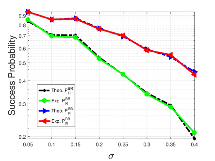
Figure 1: Average success probabilities versus $\sigma$ for $n=8$ and $\mathcal{B}=[0,3]^{n}$

V Summary

In this paper, we investigated the success probability of box-constrained rounding detectors ${\boldsymbol{x}}^{\scriptscriptstyle\text{BR}}$ and box-constrained Babai detectors ${\boldsymbol{x}}^{\scriptscriptstyle\text{BB}}$, and studied their relationship. We first proposed formulas for the success probability $P_{\scriptscriptstyle\text{D}}^{\scriptscriptstyle\text{BR}}$ and $P_{\scriptscriptstyle\text{R}}^{\scriptscriptstyle\text{BR}}$ for ${\boldsymbol{x}}^{\scriptscriptstyle\text{BR}}$, and the success probability $P_{\scriptscriptstyle\text{D}}^{\scriptscriptstyle\text{BB}}$ for ${\boldsymbol{x}}^{\scriptscriptstyle\text{BB}}$. Then, we gave an example which shows that $P_{\scriptscriptstyle\text{D}}^{\scriptscriptstyle\text{BR}}$ may strictly larger than $P_{\scriptscriptstyle\text{D}}^{\scriptscriptstyle\text{BB}}$. Finally, we rigorously showed that $P_{\scriptscriptstyle\text{R}}^{\scriptscriptstyle\text{BR}}\leq P_{\scriptscriptstyle\text{R}}^{\scriptscriptstyle\text{BB}}$ always holds if ${\hat{{\boldsymbol{x}}}}$ is uniformly distributed over the constraint box $\mathcal{B}$.