Re-interpretation of Skyrme Theory: New Topological structures

Abstract

Recently it has been pointed out that the skyrmions carry two independent topology, the baryon topology and the monopole topology. We provide more evidence to support this. In specific, we prove that the baryon number $B$ can be decomposed to the monopole number $m$ and the shell number $n$, so that $B$ is given by $B=mn$. This tells that the skyrmions may more conveniently be classified by two integers $(m,n)$. This is because the rational map which determines the baryon number in the popular multi-skyrmion solutions actually describes the monopole topology $\pi_{2}(S^{2})$ which is different from the baryon topology $\pi_{3}(S^{3})$. Moreover, we show that the baby skyrmions can also be generalized to have two topology, $\pi_{1}(S^{1})$ and $\pi_{2}(S^{2})$, and thus should be classified by two topological numbers $(m,n)$. Furthermore, we show that the vacuum of the Skyrme theory can be classified by two topological numbers $(p,q)$, the $\pi_{1}(S^{1})$ of the sigma-field and the $\pi_{3}(S^{2})$ of the normalized pion-field. This means that the Skyrme theory has multiple vacua similar to the Sine-Gordon theory and QCD combined together. This puts the Skyrme theory in a totally new perspective. We discussthe physical implications of our results.

I Introduction

The Skyrme theory has played an important role in physics. Originally it was proposed as a theory of pion physics in strong interaction where the skyrmion, a topological soliton made of pions, appears as the baryon sky . Soon after, the theory has been interpreted as a low energy effective theory of QCD in which the massless pion fields emerge as the Nambu-Goldstone field of the spontaneous chiral symmetry breaking witt ; rho ; bogo ; prep . This view has become popular and very successful.

After the Skyrme’s proposal novel way to obtain multi-skyrmions without the spherical symmetry was developed, and the skyrmions with baryon number up to 9 based on the rational map have been constructed and associated with real nuclei bat ; man . Moreover, a systematic approach utilizing the shell structure which made the numerical construction of skyrmions with large baryon number possible has been developed houg ; sut ; piet1 ; piet2 . This, with the improved computational power has made people construct skyrmions with the baryon number up to 108 sky108 .

With the new development the Skyrme theory has been able to provide a quantitative understanding of the spectrum of rotational excitations of carbon-12, including the Hoyle state which is essential for the generation of heavy nuclear elements in early universe hoyle ; epel ; lau . And the spin-orbit interaction which is essential for the magic number of nuclei is investigated within the framework of Skyrme theory hal . Moreover, a method to reduce the binding energy of skyrmions to a realistic level to improve the Skyrme model has been developed adam . So by now in principle one could construct all nuclei as multi-baryon skyrmions and discuss the phenomenology of nuclear physics.

But the Skyrme theory has multiple faces which has other topological objects. In addition to the well known skyrmion it has the (helical) baby skyrmion and the Faddeev-Niemi knot. Most importantly, it has the monopole which plays the fundamental role. In fact it can be viewed as a theory of monopole which has a built-in Meissner effect prl01 ; plb04 ; ijmpa08 . In this view all finite energy topological objects in the theory could be viewed either as dressed monopoles or as confined magnetic flux of the monopole-antimonopole pair. The skyrmion can be viewed as a dressed monopole, the baby skyrmion as a magnetic vortex created by the monopole-antimonopole pair infinitely separated apart, and the Faddeev-Niemi knot as a twisted magnetic vortex ring made of the helical baby skyrmion.

This tells that the theory can be interpreted as a theory of monopole in which the magnetic flux of the monopoles are confined and/or screened. Indeed this has made the theory very important not only in high energy physics but also in condensed matter physics, in particular in two-gap superconductor and two-component Bose-Einstein condensates plb04 ; ijmpa08 ; ruo ; pra05 ; manko .

Of course, the fact that the skyrmion is closely related to the monopole has been appreciated for a long time. It has been well known that the rational map which played the crucial role in the construction of the multi-skyrmions is exactly the $\pi_{2}(S^{2})$ mapping which provides the monopole quantum number houg . Nevertheless the skyrmions have always been classified by the baryon number given by $\pi_{3}(S^{3})$, not by the monopole number $\pi_{2}(S^{2})$. This was puzzling.

This raises a serious question on the popular view that the skyrmion can be identified as the baryon. If the skyrmions are dressed monopoles which have the monopole topology, one might wonder what is the role of the monopole in the baryon. More bluntly, we have to explain what is the connection between the monopole topology $\pi_{2}(S^{2})$ and the baryon topology $\pi_{3}(S^{3})$ which defines the baryon number $B$.

Besides, the Faddeev-Niemi knots add another problem. If we adopt the popular view the Faddeev-Niemi knots should be interpreted as topologically stable mesons made of baryon-antibaryon pair, since they could be viewed as the twisted vortex rings made of skyrmion-antiskyrmion pairs. And they are expected to have huge mass, simply because of the geometric shape prl01 ; plb04 ; ijmpa08 . This implies the existence of supermassive topologically stable mesons which might be very difficult to accommodate from the phenomenological point of view.

Recently a new proposal was made which could shed a new light on these problems. First, it was argued that the skyrmions could actually be classified by two topological numbers, the baryon number $b$ and the monopole number $m$ epjc17 . According to this proposal the baryon number could be replaced by the radial (shell) quantum number $n$ which describes the $\pi_{1}(S^{1})$ topology of the radial extension of the skyrmions. This was based on the observation that the $S^{3}$ space (both the compactified 3-dimensional real space and the SU(2) target space) has the Hopf fibering $S^{3}\simeq S^{2}\times S^{1}$, so that the baryon number defined by $\pi_{3}(S^{3})$ can be decomposed to two topological numbers $\pi_{2}(S^{2})$ and $\pi_{1}(S^{1})$.

Moreover, it has been argued that the Skyrme theory in fact has the multiple vacua similar to the Sine-Gordon theory, each of which has the knot topology of the QCD vacuum epjc17 . In other words, the vacuum of the Skyrme theory has the topology of the Sine-Gordon theory and QCD combined together. If so, the vacuum of the Skyrme theory can also be classified by two integers by $(p,q)$, $p$ which represents the $\pi_{1}(S^{1})$ topology and $q$ which represents the $\pi_{3}(S^{2})$ topology.

These new features, in particular the fact that the skyrmions can be classified by two topological quantum numbers, naturally clarifies the relation between the monopole topology and the baryon topology of the skyrmion. As importantly, the fact that the Skyrme theory has a non-trivial vacuum topology strongly suggests that the Skyrme theory really need a totally new interpretation.

On the other hand, these new features are totally unexpected, and many peoples might still be skeptical about this. The purpose of this paper is to provide more evidence to support these new features of Skyrme theory, to clarify them in more detail, and to discuss their physical implications. In particular, we present new solutions of baby skyrmion, and show that (not only the skyrmion but also) the baby skyrmion has two topology, the shell (radial) topology $\pi_{1}(S^{1})$ and the monopole topology $\pi_{2}(S^{2})$. This means that the baby skyrmion should also be classified by two topological numbers. This is really remarkable, which strongly support that the skyrmion does carry two topology.

The paper is organized as follows. In Section II we briefly review the old skyrmions for later purpose. In Section III we reveal the hidden connection between the Skyrme theory and QCD, and emphasize that the skyrmion is the dressed Wu-Yang monopole of QCD transplanted in the Skyrme theory. In Section IV we show that the skyrmions carry two topological quantum numbers, the baryon number $b$ and the monopole number $m$. Moreover, we show that the baryon number can be replaced by the radial (shell) quantum number $n$, so that they can be classified by $(m,n)$ In this scheme the baryon number is given by $b=mn$. In Section V we obtain new baby skyrmion solutions, and show how the baby skyrmion can be generalized to carry two topology, the radial topology $\pi_{1}(S^{1})$ and the monopole topology $\pi_{2}(S^{2})$. With this we present the baby skyrmion solutions which carry two topological numbers. In SectionVI we discuss the vacuum structure of the Skyrme theory, and show that it has the structure of the vacuum of the Sine-Gordon theory combined with the vacuum of the SU(2) QCD. This tells that it can be classified by two topological quantum numbers denoted by $(p,q)$, where $p$ and $q$ represent the $\pi_{1}(S^{1})$ topology of the Sine-Gordon theory and the $\pi_{3}(S^{2})$ topology of QCD vacuum. Finally in Section VI we discuss the physical implications of our results.

II Skyrme Theory: A Review

Before we show that the skyrmions can be classified by two quantum numbers, we first review the well known facts in Skyrme theory. Let $\omega$ and $\hat{n}$ (${\hat{n}}^{2}=1$) be the massless scalar field (the “sigma-field”) and the normalized pion-field in Skyrme theory, and write the Skyrme Lagrangian as sky

$${\cal L}=\dfrac{\kappa^{2}}{4}{\rm tr}~{}L_{\mu}^{2}+\dfrac{\alpha}{32}{\rm tr}\left(\left[L_{\mu},L_{\nu}\right]\right)^{2}$$

$$=-\dfrac{\kappa^{2}}{4}\Big{[}\dfrac{1}{2}(\partial_{\mu}\omega)^{2}+2\sin^{2}\dfrac{\omega}{2}(\partial_{\mu}\hat{n})^{2}\Big{]}$$

$$-\dfrac{\alpha}{8}\Big{[}\sin^{2}\dfrac{\omega}{2}\big{(}(\partial_{\mu}\omega)^{2}(\partial_{\nu}\hat{n})^{2}-(\partial_{\mu}\omega\partial_{\nu}\omega)(\partial_{\mu}\hat{n}\cdot\partial_{\nu}\hat{n})\big{)}$$

$$+2\sin^{4}\dfrac{\omega}{2}(\partial_{\mu}\hat{n}\times\partial_{\nu}\hat{n})^{2}\Big{]},$$

$$L_{\mu}=U\partial_{\mu}U^{\dagger},$$

$$U=\exp(\dfrac{\omega}{2i}\vec{\sigma}\cdot\hat{n})=\cos\dfrac{\omega}{2}-i(\vec{\sigma}\cdot\hat{n})\sin\dfrac{\omega}{2},$$ (1)

where $\kappa$ and $\alpha$ are the coupling constants. The Lagrangian has a hidden $U(1)$ gauge symmetry which leaves $\hat{n}$ invariant as well as a global $SU(2)_{L}\times SU(2)_{R}$ symmetry.

Notice that, with

$$\sigma=\cos\dfrac{\omega}{2},~{}~{}~{}\vec{\pi}=\hat{n}\sin\dfrac{\omega}{2},~{}~{}~{}(\sigma^{2}+\vec{\pi}^{2}=1),$$ (2)

the Lagrangian (1) can also be put into the form

$${\cal L}=-\dfrac{\kappa^{2}}{2}\big{(}(\partial_{\mu}\sigma)^{2}+(\partial_{\mu}\vec{\pi})^{2}\big{)}$$

$$-\dfrac{\alpha}{4}\big{(}(\partial_{\mu}\sigma\partial_{\nu}\vec{\pi}-\partial_{\nu}\sigma\partial_{\mu}\vec{\pi})^{2}+(\partial_{\mu}\vec{\pi}\times\partial_{\nu}\vec{\pi})^{2}\big{)}$$

$$+\dfrac{\lambda}{4}(\sigma^{2}+\vec{\pi}^{2}-1),$$ (3)

where $\lambda$ is a Lagrange multiplier. In this form $\sigma$ and $\vec{\pi}$ represent the sigma field and the pion field, so that the theory describes the non-linear sigma model of the pion physics.

The Lagrangian has a hidden $U(1)$ gauge symmetry as well as the global $SU(2)_{L}\times SU(2)_{R}$ symmetry plb04 ; ijmpa08 . The global $SU(2)_{L}\times SU(2)_{R}$ symmetry is obvious, but the hidden $U(1)$ gauge symmetry is not. The hidden $U(1)$ gauge symmetry comes from the $U(1)$ subgroup which leaves $\hat{n}$ invariant. To see this, we reparametrize $\hat{n}$ by the $CP^{1}$ field $\xi$,

$$\vec{n}=\xi^{\dagger}\vec{\sigma}\xi,~{}~{}~{}~{}~{}\xi^{\dagger}\xi=1.$$ (4)

and find that under the $U(1)$ gauge transformation of $\xi$ to

$$\xi\rightarrow\exp(i\theta(x))\xi,$$ (5)

$\hat{n}$ (and $\partial_{\mu}\hat{n}$) remains invariant. Now, we introduce the composite gauge potential $C_{\mu}$ and the covariant derivative $D_{\mu}$ which transforms gauge covariantly under (5) by

$$C_{\mu}=-2i\xi^{\dagger}\partial_{\mu}\xi,~{}~{}~{}D_{\mu}\xi=(\partial_{\mu}-\frac{i}{2}C_{\mu})\xi.$$ (6)

With this we have the following identities,

$$(\partial_{\mu}\hat{n})^{2}=4|D_{\mu}\xi|^{2},$$

$$\partial_{\mu}\hat{n}\times\partial_{\nu}\hat{n}=-2i\Big{[}(\partial_{\mu}\xi^{\dagger})(\partial_{\nu}\xi)-(\partial_{\mu}\xi^{\dagger})(\partial_{\nu}\xi)\Big{]}\hat{n}$$

$$=H_{\mu\nu}\hat{n},$$

$$H_{\mu\nu}=\partial_{\mu}C_{\nu}-\partial_{\nu}C_{\mu}.$$ (7)

Furthermore, with the Fierz’ identity

$$\sigma_{ij}^{a}\sigma_{kl}^{a}=2\delta_{il}\delta_{jk}-\delta_{ij}\delta_{kl},$$ (8)

we have

$$\partial_{\mu}\hat{n}\cdot\partial_{\mu}\hat{n}=2\partial_{\mu}(\xi^{\dagger}_{i}\xi_{j})\partial_{\nu}(\xi^{\dagger}_{j}\xi_{i})$$

$$=2\Big{[}(\partial_{\mu}\xi^{\dagger}\xi)(\partial_{\nu}\xi^{\dagger}\xi)+(\partial_{\mu}\xi^{\dagger})(\partial_{\nu}\xi)+(\partial_{\nu}\xi^{\dagger})(\partial_{\mu}\xi)$$

$$+(\xi^{\dagger}\partial_{\mu}\xi)(\xi^{\dagger}\partial_{\nu}\xi)\Big{]}=2\Big{[}(\partial_{\mu}\xi^{\dagger}+\frac{i}{2}C_{\mu}\xi^{\dagger})(\partial_{\nu}\xi-\frac{i}{2}C_{\nu}\xi)$$

$$+(\partial_{\nu}\xi^{\dagger}+\frac{i}{2}C_{\nu}\xi^{\dagger})(\partial_{\mu}\xi-\frac{i}{2}C_{\mu}\xi)\Big{]}$$

$$=2\Big{[}(D_{\mu}\xi)^{\dagger}(D_{\nu}\xi)+(D_{\nu}\xi)^{\dagger}(D_{\mu}\xi)\Big{]}.$$ (9)

From this we can express (1) by

$${\cal L}=-\dfrac{\kappa^{2}}{4}\Big{[}\dfrac{1}{2}(\partial_{\mu}\omega)^{2}+8\sin^{2}\dfrac{\omega}{2}|D_{\mu}\xi|^{2}\Big{]}$$

$$-\dfrac{\alpha}{2}\sin^{2}\dfrac{\omega}{2}\Big{[}(\partial_{\mu}\omega)^{2}|D_{\mu}\xi|^{2}-(\partial_{\mu}\omega\partial_{\nu}\omega)(D_{\mu}\xi)^{\dagger}(D_{\nu}\xi)$$

$$+\frac{1}{2}\sin^{2}\dfrac{\omega}{2}H_{\mu\nu}^{2}\Big{]},$$ (10)

which is explicitly invariant under the $U(1)$ gauge transformation (5). So replacing $\hat{n}$ by $\xi$ in the Lagrangian we can make the hidden $U(1)$ gauge symmetry explicit. In this form the Skyrme theory becomes a self-interacting $U(1)$ gauge theory of $CP^{1}$ field coupled to a massless scalar field.

The Lagrangian gives the following equations of motion

$$\partial^{2}\omega-\sin\omega(\partial_{\mu}\hat{n})^{2}+\dfrac{\alpha}{8\kappa^{2}}\sin\omega(\partial_{\mu}\omega\partial_{\nu}\hat{n}-\partial_{\nu}\omega\partial_{\mu}\hat{n})^{2}$$

$$+\dfrac{\alpha}{\kappa^{2}}\sin^{2}\dfrac{\omega}{2}\partial_{\mu}\big{[}(\partial_{\mu}\omega\partial_{\nu}\hat{n}-\partial_{\nu}\omega\partial_{\mu}\hat{n})\cdot\partial_{\nu}\hat{n}\big{]}$$

$$-\dfrac{\alpha}{\kappa^{2}}\sin^{2}\dfrac{\omega}{2}\sin\omega(\partial_{\mu}\hat{n}\times\partial_{\nu}\hat{n})^{2}=0,$$

$$\partial_{\mu}\Big{\{}\sin^{2}\dfrac{\omega}{2}\hat{n}\times\partial_{\mu}\hat{n}+\dfrac{\alpha}{4\kappa^{2}}\sin^{2}\dfrac{\omega}{2}\big{[}(\partial_{\nu}\omega)^{2}\hat{n}\times\partial_{\mu}\hat{n}$$

$$-(\partial_{\mu}\omega\partial_{\nu}\omega)\hat{n}\times\partial_{\nu}\hat{n}\big{]}$$

$$+\dfrac{\alpha}{\kappa^{2}}\sin^{4}\dfrac{\omega}{2}(\hat{n}\cdot\partial_{\mu}\hat{n}\times\partial_{\nu}\hat{n})\partial_{\nu}\hat{n}\Big{\}}=0.$$ (11)

Notice that the second equation can be interpreted as the conservation of $SU(2)$ current originating from the global $SU(2)$ symmetry of the theory.

It has two interesting limits. First, when

$$\omega=(2p+1)\pi,$$ (12)

(11) is reduced to

$$\hat{n}\times\partial^{2}\hat{n}-\dfrac{\alpha}{\kappa^{2}}(\partial_{\mu}H_{\mu\nu})\partial_{\nu}\hat{n}=0,$$

$$H_{\mu\nu}=\hat{n}\cdot(\partial_{\mu}\hat{n}\times\partial_{\nu}\hat{n})=\partial_{\mu}C_{\nu}-\partial_{\nu}C_{\mu},$$ (13)

where $C_{\mu}$ is the magnetic potential of $H_{\mu\nu}$ defined by (6). This is the central equation of Skyrme theory which allows the monopole, the baby skyrmion, and the Faddeev-Niemi knot prl01 ; plb04 ; ijmpa08 .

Second, in the spherically symmetric limit

$$\omega=\omega(r),~{}~{}~{}~{}~{}\hat{n}=\pm\hat{r},$$ (14)

(11) is reduced to

$$\dfrac{d^{2}\omega}{dr^{2}}+\dfrac{2}{r}\dfrac{d\omega}{dr}-\dfrac{2\sin\omega}{r^{2}}+\dfrac{2\alpha}{\kappa^{2}}\Big{[}\dfrac{\sin^{2}(\omega/2)}{r^{2}}\dfrac{d^{2}\omega}{dr^{2}}$$

$$+\dfrac{\sin\omega}{4r^{2}}(\dfrac{d\omega}{dr})^{2}-\dfrac{\sin\omega\sin^{2}(\omega/2)}{r^{4}}\Big{]}=0.$$ (15)

This is the equation used by Skyrme to find the original skyrmion. Imposing the boundary condition

$$\omega(0)=2\pi,~{}~{}~{}~{}~{}\omega(\infty)=0,$$ (16)

we have the skyrmion solution which carries the unit baryon number sky

$$B=-\dfrac{1}{24\pi^{2}}{\displaystyle\int}\epsilon_{ijk}~{}{\rm tr}~{}(L_{i}L_{j}L_{k})d^{3}r$$

$$=-\dfrac{1}{8\pi^{2}}\int\epsilon_{ijk}\partial_{i}\omega\big{[}\hat{r}\cdot(\partial_{j}\hat{r}\times\partial_{k}\hat{r})\big{]}\sin^{2}\dfrac{\omega}{2}d^{3}r$$

$$=1,$$ (17)

which represents the non-trivial homotopy $\pi_{3}(S^{3})$ defined by $U$.

The two limits lead us to very interesting physics. To understand the physical meaning of the first limit notice that, with (12) the Skyrme Lagrangian reduces to the Skyrme-Faddeev Lagrangian

$${\cal L}\rightarrow-\dfrac{\kappa^{2}}{2}(\partial_{\mu}\hat{n})^{2}-\dfrac{\alpha}{4}(\partial_{\mu}\hat{n}\times\partial_{\nu}\hat{n})^{2},$$ (18)

whose equation of motion is given by (13). This tells that the Skyrme-Faddeev theory becomes a self-consistent truncation of the Skyrme theory. This assures that the Skyrme-Faddeev theory is an essential ingredient (the backbone) of the Skyrme theory which describes the core dynamics of Skyrme theory prl01 ; plb04 ; ijmpa08 .

A remarkable feature of the Skyrme-Faddeev theory is that it can be viewed as a theory of monopole. In fact, (13) has the singular monopole solution prl01 ; plb04 ; ijmpa08

$$\hat{n}=\pm\hat{r}.$$ (19)

which carries the magnetic charge

$$Q_{m}=\dfrac{\pm 1}{8\pi}\int\epsilon_{ijk}\big{[}\hat{r}\cdot(\partial_{i}\hat{r}\times\partial_{j}\hat{r})\big{]}d\sigma_{k}=\pm 1,$$ (20)

which represents the homotopy $\pi_{2}(S^{2})$ defined by $\hat{n}$. Of course, (19) has a point singularity at the origin which makes the energy divergent. But we can easily regularize the singularity with a non-trivial $\omega$, with the boundary condition (16). And the regularized monopole becomes nothing but the well known skyrmion prl01 ; plb04 ; ijmpa08 .

Moreover, it has the (helical) magnetic vortex solution made of the monopole-antimonopole pair infinitely separated apart, and the knot solution which can be viewed as the twisted magnetic vortex ring made of the helical vortex whose periodic ends are connected together. So the monopole plays an essential role in all these solutions. This shows that the Skyrme-Faddeev theory, and by implication the Skyrme theory itself, can be viewed as a theory of monopole.

But perhaps a most important point of the Skyrme-Faddeev Lagrangian is that it provides a “missing” link between Skyrme theory and QCD, because the Skyrme-Faddeev Lagrangian can actually be derived from QCD prl01 ; plb04 ; ijmpa08 .

III Skyrme Theory and QCD: A Theory of Monopole

To reveal the deep connection between Skyrme theory and QCD, consider the SU(2) QCD

$${\cal L}_{QCD}=-\dfrac{1}{4}\vec{F}_{\mu\nu}^{2}.$$ (21)

Now, we can make the Abelian projection choosing the Abelian direction to be $\hat{n}$ and imposing the Abelian isometry

$$D_{\mu}\hat{n}=0,$$ (22)

to the gauge potential. With this we obtain the restricted potential $\hat{A}_{\mu}$ which describes the color neutral binding gluon (the neuron) prd80 ; prl81

$${\vec{A}}_{\mu}\rightarrow\hat{A}_{\mu}={\cal A}_{\mu}+{\cal C}_{\mu},$$

$${\cal A}_{\mu}=A_{\mu}\hat{n},~{}~{}~{}{\cal C}_{\mu}=-\dfrac{1}{g}\hat{n}\times\partial_{\mu}\hat{n}.$$ (23)

The restricted potential is made of two parts, the naive Abelian (Maxwellian) part ${\cal A}_{\mu}$ and the topological monopole (Diracian) part ${\cal C}_{\mu}$. Moreover, it has the full non-Abelian gauge freedom although the holonomy group of the restricted potential is Abelian.

So we can construct the restricted QCD (RCD) made of the restricted potential which has the full SU(2) gauge freedom prd80 ; prl81

$${\cal L}_{RCD}=-\dfrac{1}{4}\hat{F}^{2}_{\mu\nu}=-\dfrac{1}{4}(F_{\mu\nu}-\dfrac{1}{g}H_{\mu\nu})^{2}$$

$$=-\dfrac{1}{4}F_{\mu\nu}^{2}+\dfrac{1}{2g}F_{\mu\nu}\hat{n}\cdot(\partial_{\mu}\hat{n}\times\partial_{\nu}\hat{n})-\dfrac{1}{4g^{2}}(\partial_{\mu}\hat{n}\times\partial_{\nu}\hat{n})^{2},$$

$$F_{\mu\nu}=\partial_{\mu}A_{\nu}-\partial_{\nu}A_{\mu},~{}~{}~{}H_{\mu\nu}=\partial_{\mu}C_{\nu}-\partial_{\nu}C_{\mu}.$$ (24)

This shows that RCD is a dual gauge theory made of two Abelian gauge potentials, the electric $A_{\mu}$ and magnetic $C_{\mu}$. Nevertheless it has the full non-Abelian gauge symmetry.

Moreover, we can recover the full SU(2) QCD with the Abelian decomposition which decomposes the gluons to the color neutral neuron and colored chromon gauge independently prd80 ; prl81

$${\vec{A}}_{\mu}=\hat{A}_{\mu}+\vec{X}_{\mu},~{}~{}~{}\hat{n}\cdot\vec{X}_{\mu}=0,$$

$$\vec{F}_{\mu\nu}=\hat{F}_{\mu\nu}+{\hat{D}}_{\mu}{\vec{X}}_{\nu}-{\hat{D}}_{\nu}{\vec{X}}_{\mu}+g{\vec{X}}_{\mu}\times{\vec{X}}_{\nu},$$ (25)

where $\vec{X}_{\mu}$ describes the gauge covariant colored chromon. With this we have the Abelian decomposition of QCD

$${\cal L}_{QCD}=-\dfrac{1}{4}\vec{F}^{2}_{\mu\nu}=-\dfrac{1}{4}\hat{F}_{\mu\nu}^{2}-\dfrac{1}{4}({\hat{D}}_{\mu}{\vec{X}}_{\nu}-{\hat{D}}_{\nu}{\vec{X}}_{\mu})^{2}$$

$$-\dfrac{g}{2}{\hat{F}}_{\mu\nu}\cdot({\vec{X}}_{\mu}\times{\vec{X}}_{\nu})-\dfrac{g^{2}}{4}({\vec{X}}_{\mu}\times{\vec{X}}_{\nu})^{2}.$$ (26)

This confirms that QCD can be viewed as RCD made of the binding gluon, which has the colored valence gluon as its source prd80 ; prl81 .

Now we can reveal the connection between the Skyrme theory and QCD. Let us start from RCD and assume that the binding gluon (restricted potential) acquires a mass term after the confinement. In this case (24) becomes

$${\cal L}_{RCD}\rightarrow-\dfrac{1}{4}\hat{F}^{2}_{\mu\nu}-\dfrac{m^{2}}{2}\hat{A}_{\mu}^{2}$$

$$=-\dfrac{1}{4}F_{\mu\nu}^{2}+\dfrac{1}{2g}F_{\mu\nu}\hat{n}\cdot(\partial_{\mu}\hat{n}\times\partial_{\nu}\hat{n})$$

$$-\dfrac{1}{4g^{2}}(\partial_{\mu}\hat{n}\times\partial_{\nu}\hat{n})^{2}-\dfrac{m^{2}}{2}\big{[}A_{\mu}^{2}+(\partial_{\mu}\hat{n})^{2}\big{]}.$$ (27)

Of course, the mass term breaks the gauge symmetry, but this can be justified because the binding gluons could acquire mass after the confinement sets in.

Integrating out the $A_{\mu}$ potential (or simply putting $A_{\mu}=0$), we can reduce (27) to

$${\cal L}_{RCD}\rightarrow-\dfrac{1}{4g^{2}}(\partial_{\mu}\hat{n}\times\partial_{\nu}\hat{n})^{2}-\dfrac{m^{2}}{2}(\partial_{\mu}\hat{n})^{2},$$ (28)

which becomes nothing but the Skyrme-Faddeev Lagrangian (18) when $\kappa^{2}=m^{2}$ and $\alpha=1/g^{2}$. This tells that the Skyrme-Faddeev Lagrangian can actually be derived from RCD. And this is a mathematical derivation. This confirms that the Skyrme theory and QCD is closely related, more closely than it appears.

This has deep consequences. Notice that $\hat{n}$ which provides the Abelian projection in QCD naturally represents the monopole topology $\pi_{2}(S^{2})$, and can describe the monopole. In fact, it is well known that $\hat{n}=\hat{r}$ becomes exactly the Wu-Yang monopole solution prd80 ; prl81 ; prl80 . On the other hand the above exercise tells that this $\hat{n}$ is nothing but the normalized pion field in the Skyrme theory. This strongly implies that $\hat{n}=\hat{r}$ can also describe the monopole solution in the Skyrme theory. Indeed, (19) is precisely the Wu-Yang monopole transplanted in the Skyrme theory.

What is more, the Skyrme theory has more complicated monopole solutions. With $\hat{n}=\hat{r}$ and the boundary condition

$$\omega(0)=\pi,~{}~{}~{}~{}\omega(\infty)=0,~{}~{}~{}~{}({\rm mod}~{}2\pi)$$ (29)

we can find a monopole solution which reduces to the singular solution (19) near the origin. The only difference between this and (19) is the non-trivial dressing of the scalar field $\omega$, so that it could be interpreted as a dressed monopole. This dressing, however, is only partial because this makes the energy finite at the infinity, but not at the origin.

Similarly, with the following boundary condition

$$\omega(0)=2\pi,~{}~{}~{}~{}\omega(\infty)=\pi,~{}~{}~{}~{}({\rm mod}~{}2\pi)$$ (30)

we can obtain another monopole and half-skyrmion solution which approaches the singular solution near the infinity. Here again the partial dressing makes the energy finite at the origin, but not at the infinity. So the partially dressed monopoles still carry an infinite energy.

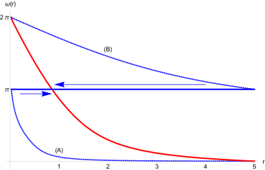
Figure 1: The singular Wu-Yang monopole (the blue line), the two half skyrmions (A) and (B) as partially dressed singular monopoles (blue curves), and the regular skyrmion (red curve) obtained combining the two half skyrmions.

Clearly these solutions carry the unit magnetic charge of the homotopy $\pi_{2}(S^{2})$ defined by $\hat{n}$ ijmpa08

$$M=\dfrac{\pm 1}{8\pi}\int\epsilon_{ijk}\big{[}\hat{r}\cdot(\partial_{i}\hat{r}\times\partial_{j}\hat{r})\big{]}d\sigma_{k}=\pm 1,$$ (31)

but carry a half baryon number

$$B=-\dfrac{1}{8\pi^{2}}\int\epsilon_{ijk}\partial_{i}\omega\big{[}\hat{r}\cdot(\partial_{j}\hat{r}\times\partial_{k}\hat{r})\big{]}\sin^{2}\dfrac{\omega}{2}d^{3}r$$

$$=-\dfrac{1}{\pi}\int\sin^{2}\dfrac{\omega}{2}d\omega=\dfrac{1}{2}.$$ (32)

This is due to the boundary conditions (29) and (30). So it describes a half-skyrmion.

The half-skyrmions have two remarkable features. First, combining the two half-skyrmions we can form a finite energy soliton, the fully dressed skyrmion ijmpa08 . This must be clear because, putting the boundary conditions (29) and (30) together we recover the boundary condition (16) of the skyrmion. So putting the two partially dressed monopoles together we obtain the well known finite energy skyrmion solution.

This is summarized in Fig. 1, where the blue line represents the singular monopole, the dotted curves (A) and (B) represent the singular half skyrmions, and the red curve represents the regular skyrmion. Notice that in all these solutions we have $\hat{n}=\hat{r}$, so that $M=1$. This confirms that the skyrmion is nothing but the Wu-Yang monopole of QCD, transplanted and regularized to have a finite energy by the massless scalar field $\omega$ in the Skyrme theory prl01 ; plb04 ; ijmpa08 .

The other remarkable feature of the half-skyrmions is that the monopole number (31) and the baryon number (32) are different. This is very interesting because, in skyrmions the baryon number is commonly identified by the rational map which defines the monopole number. This suggests that the baryon number and the monopole number are one and the same thing houg . But obviously this is not true for the half-skyrmions. In the following we will argue that this need not be ture, and show that the skyrmions in general have two different topological numbers.

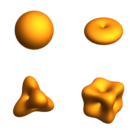
Figure 2: The well known (non spherically symmetric) numerical multi-skyrmion solutions with baryon number 1,2,3,4.

IV A New Classification of Skyrmion

The above argument clearly shows that the skyrmion has the monopole topology. And this monopole topology reappear in all popular non spherically symmetric multi-skyrmion solutions man ; bat ; houg ; sut ; piet1 ; piet2 . Indeed, it is well known that the monopole topology of the rational map $\pi_{2}(S^{2})$ given by $\hat{n}$,

$$M=\dfrac{1}{8\pi}\int\epsilon_{ijk}\big{[}\hat{n}\cdot(\partial_{i}\hat{n}\times\partial_{j}\hat{n})\big{]}d\sigma_{k}=m,$$ (33)

together with the boundary condition (16), has played the fundamental role for many people to construct these multi-skyrmion solutions. Some of these multi-skyrmion solutions are shown in Fig. 2.

On the other hand, these solutions have always been interpreted to have the baryon topology $\pi_{3}(S^{3})$ which have the baryon number given by

$$B=-\dfrac{1}{8\pi^{2}}\int\epsilon_{ijk}\partial_{i}\omega\big{[}\hat{n}\cdot(\partial_{j}\hat{n}\times\partial_{k}\hat{n})\big{]}\sin^{2}\dfrac{\omega}{2}d^{3}r$$

$$=\dfrac{1}{8\pi}\int\epsilon_{ijk}\big{[}\hat{n}\cdot(\partial_{i}\hat{n}\times\partial_{j}\hat{n})\big{]}d\sigma_{k}=m.$$ (34)

But obviously this baryon number is precisely the monopole number shown in (33), so that these solutions have $B=M$. Nevertheless, the monopole topology $\pi_{2}(S^{2})$ and the baryon topology $\pi_{3}(S^{3})$ is clearly different. If so, we may ask what is the relation between the monopole topology and the baryon topology.

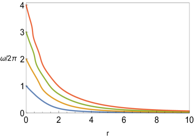
Figure 3: The spherically symmetric skyrmions with baryon number 1,2,3,4, which should be contrasted with the solutions shown in Fig. 2.

The Skyrme equation (15) in the spherically symmetric limit plays an important role to clarify this point. To see this notice that, although the SU(2) matrix $U$ is periodic in $\omega$ variable by $4\pi$, $\omega$ itself can take any value from $-\infty$ to $+\infty$. So we can obtain the spherically symmetric multi-skyrmion solutions generalizing the boundary condition (16) to sky ; witt ; rho ; bogo ; prep

$$\omega(0)=2\pi n,~{}~{}~{}~{}~{}\omega(\infty)=0,$$ (35)

with an arbitrary integer $n$. Some of the spherically symmetric multi-skyrmion solutions are shown in Fig. 3. These are, of course, the solutions that Skyrme originally proposed to identify as the nuclei with baryon number larger than one sky ; rho . But soon after they are dismissed as uninteresting because they have too much energy.

An interesting features of the spherically symmetric solutions is that whenever the curve passes through the values $\omega=2\pi n$, it become a bit steeper. This is because (as we will see soon) these points are the vacua of the theory, and the steep slopes shows that the energy likes to be concentrated around these vacua.

Another interesting feature of the spherically symmetric skyrmions is the energy, which is given by ijmpa08

$$E=\dfrac{\pi\kappa^{2}}{2}{\displaystyle\int}_{0}^{\infty}\Big{\{}\Big{(}r^{2}+\dfrac{2\alpha}{\kappa^{2}}\sin^{2}\dfrac{\omega}{2}\Big{)}\Big{(}\dfrac{d\omega}{dr}\Big{)}^{2}$$

$$+8\Big{(}1+\dfrac{\alpha}{2\kappa^{2}r^{2}}\sin^{2}\dfrac{\omega}{2}\Big{)}\sin^{2}\dfrac{\omega}{2}\Big{\}}dr$$

$$=\pi{\sqrt{\alpha}}\kappa{\displaystyle\int}^{\infty}_{0}\Big{[}x^{2}\left(\dfrac{d\omega}{dx}\right)^{2}+8\sin^{2}{\dfrac{\omega}{2}}\Big{]}dx,$$ (36)

where $x=\kappa r/{\sqrt{\alpha}}$. From this we can easily calculate their energy. This is shown in Fig. 4.

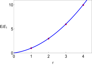
Figure 4: The energy of the spherically symmetric solutions with baryon number 1,2,3,4. The numerical fit (the blue curve) and the $n(n+1)E_{1}/2$ curve (the green curve) are almost indistinguishable.

Numerically the baryon number dependence of the energy is given by rho ; bogo ; prep

$$E_{n}\simeq\dfrac{n(n+1)}{2}E_{1}.$$ (37)

This has two remarkable points. First, the baryon number dependence of the energy is quadratic. This, of course, means that the energy of the skyrmion with baryon number $n$ is bigger than the sum of $n$ lowest energy skyrmion. So the radially excited skyrmions are unstable. This is not the case in the popular multi-skyrmion solutions shown in Fig. 2. They have positive binding energy, so that the energy of the skyrmion with baryon number $B$ becomes smaller than the $B$ sum of the lowest energy skyrmion. This was the main reason why the spherically symmetric solutions have not been considered seriously as the model of heavy nuclei.

But actually (37) makes the spherically symmetric solutions mathematically more interesting, because (37) is almost exact. In fact Fig. 4 shows that the mathematical curve $E_{n}=n(n+1)E_{1}/2$ and the numerical fit is almost indistinguishable. Intuitively this could be understood as follows. Roughly speaking, the kinetic energy (first part) and the potential energy (second part) of (36) become proportional to $n^{2}$ and $n$, and the two terms have an equal contribution due to the equipartition of energy. But the truth is more complicated than this, and we certainly need a mathematical explanation of (37).

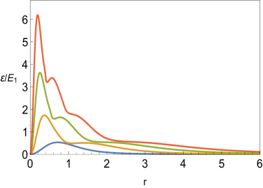
Figure 5: The radial energy density of the spherically symmetric skyrmions with baryon number 1,2,3,4. The density functions are normalized to make the integral of the $B=1$ solution to be the unit.

The energy density of the solutions is shown in Fig. 5. Clearly the $B=n$ solution has $n$ local maxima, which indicates that it is made of n shells of unit skyrmions. Moreover, as we have remarked the energy density has the local maxima at $\omega=2\pi n$. So they describe the shell model of nuclei, made of $n$ shells located at $\omega=2\pi n$. This tells that the spherically symmetric solutions could be viewed as radially extended skyrmions of the original skyrmion. In this interpretation the baryon number $n$ of these skyrmions can be identified as the radial, or more properly the shell, number piet1 ; piet2 . And this baryon number is fixed by the winding number $\pi_{1}(S^{1})$ of the angular variable $\omega$.

The contrast between the popular non spherically symmetric solutions shown in Fi‍g. 2 and the sphrically symmetric solutions shown in Fig. 3 is unmistakable. But the contrast is not just in the appearance. They are fundamentally different. In particular, the spherically symmetric solutions have a very important implication.

To understand this, notice that these solutions have the monopole number given by

$$M=\dfrac{1}{8\pi}\int\epsilon_{ijk}\big{[}\hat{r}\cdot(\partial_{i}\hat{r}\times\partial_{j}\hat{r})\big{]}d\sigma_{k}=1.$$ (38)

On the other hand, their baryon number is given by the winding number $\pi_{1}(S^{1})$ of $\omega$ determined by the boundary condition (35),

$$B=-\dfrac{1}{8\pi^{2}}\int\epsilon_{ijk}\partial_{i}\omega\big{[}\hat{r}\cdot(\partial_{j}\hat{r}\times\partial_{k}\hat{r})\big{]}\sin^{2}\dfrac{\omega}{2}d^{3}r$$

$$=-\dfrac{1}{\pi}\int\sin^{2}\dfrac{\omega}{2}d\omega=n.$$ (39)

So, unlike the popular non spherically symmetric multi-skyrmions shown in Fig. 2, the baryon number and the monopole number of these solutions are different. Moreover, the baryon number is not given by the rational map, but by the winding number.

This confirms that the skyrmions actually do carry two topological numbers, the baryon number of $\pi_{3}(S^{3})$ and the monopole number of $\pi_{2}(S^{2})$ epjc17 . And the spherically symmetric solutions play the crucial role to demonstrate this.

In this scheme the skyrmions are classified by $(m,b)$, by the monopole number $m$ and the baryon number $b$. And the popular (non spherically symmetric) solutions become the $(m,m)$ skyrmions and the spherically symmetric solutions become the $(1,n)$ skyrmions.

This has a deep consequence. Based on this we can actually show that the baryon number can be decomposed to the monopole number and the radial (shell) number and expressed by the product of the two numbers epjc17 . To show this we discuss the characteristic features of the spherically symmetric solutions first.

This implies that we could replace the baryon number with the shell number, and classify the skyrmions by the monopole number $m$ and shell number $n$ by $(m,n)$, instead of $(m,b)$. In other words we could also classify the skyrmions by the monopole topology $\pi_{2}(S^{2})$ of $\hat{n}$ and the U(1) (i.e., shell) topology $\pi_{1}(S^{1})$ of $\omega$. In this scheme the baryon number of the $(m,n)$ skyrmion is given by $B=mn$. This must be clear from (17), which tells that the baryon number is made of two parts, the $\pi_{2}(S^{2})$ of $\hat{n}$ and $\pi_{1}(S^{1})$ of $\omega$.

According to this classification the popular (non spherically symmetric) skyrmions become the $(m,1)$ skyrmions, the radially extended spherically symmetric skyrmions become the $(1,n)$ skyrmions. The justification for this classification comes from the following observation. First, the $S^{3}$ space (both the real space and the target space) in the baryon topology $\pi_{3}(S^{3})$ admits the Hopf fibering $S^{3}\simeq S^{2}\times S^{1}$. Second, the two variables $\hat{n}$ and $\omega$ of the Skyrme theory naturally accommodate the monopole topology $\pi_{2}(S^{2})$ and the shell topology $\pi_{1}(S^{1})$.

Furthermore, in this classification the baryon number is given by the product of the monopole number and the shell number, or $B=mn$. To see this notice that the Hopf fibering of $S^{3}$ has an important property that locally it can be viewed as a Cartesian product of $S^{2}$ and $S^{1}$. So we have

$$B=-\dfrac{1}{8\pi^{2}}{\displaystyle\int}\epsilon_{ijk}\partial_{i}\omega\big{[}\hat{n}\cdot(\partial_{j}\hat{n}\times\partial_{k}\hat{n})\big{]}\sin^{2}\dfrac{\omega}{2}d^{3}r$$

$$=-\dfrac{1}{8\pi^{2}}{\displaystyle\int}\partial_{i}\omega\big{[}\hat{n}\cdot(\partial_{j}\hat{n}\times\partial_{k}\hat{n})\big{]}\sin^{2}\dfrac{\omega}{2}dx^{i}\wedge dx^{j}\wedge dx^{k}$$

$$=-\dfrac{1}{8\pi^{2}}{\displaystyle\int}\sin^{2}\dfrac{\omega}{2}d\omega\times\epsilon_{ijk}\big{[}\hat{n}\cdot(\partial_{i}\hat{n}\times\partial_{j}\hat{n})\big{]}d\Sigma_{k}$$

$$=\dfrac{n}{8\pi}{\displaystyle\int}\epsilon_{ijk}\big{[}\hat{n}\cdot(\partial_{i}\hat{n}\times\partial_{j}\hat{n})\big{]}d\Sigma_{k}=mn,$$ (40)

where $d\Sigma_{k}=\epsilon_{ijk}dx^{i}\wedge dx^{j}/2$. Clearly the last integral is topologically equivalent to (19), which assures the last equality. This shows that the baryon number of the skyrmion is given by the product of the monopole number and the shell number. Obviously both $(m,1)$ and $(1,n)$ skyrmions are the particular examples of this.

Another way to show this is to introduce a generalized coordinates $(\eta,\alpha,\beta)$ for $R^{3}$ whose line element is given by fab

$$ds^{2}=f(\eta)d\eta^{2}+d\Sigma^{2}(\alpha,\beta),$$ (41)

in which $\eta$ represents the radial coordinate $R^{1}$ and $(\alpha,\beta)$ represents the $S^{2}$ such that $\omega=\omega(\eta)$ and $\hat{n}=\hat{n}(\alpha,\beta)$. Again this is possible because the hopf fibering of $S^{3}$ can be expressed by a locally Cartesian product of $S^{2}$ and $S^{1}$. In this coordinates we clearly have

$$B=-\dfrac{1}{8\pi^{2}}{\displaystyle\int}\epsilon_{ijk}\partial_{i}\omega\big{[}\hat{n}\cdot(\partial_{j}\hat{n}\times\partial_{k}\hat{n})\big{]}\sin^{2}\dfrac{\omega}{2}d^{3}x$$

$$=-\dfrac{1}{8\pi^{2}}{\displaystyle\int}\sin^{2}\dfrac{\omega}{2}\frac{d\omega}{d\eta}$$

$$\times 2{\displaystyle\int}\big{[}\hat{n}\cdot(\frac{\partial\hat{n}}{\partial\alpha}\times\frac{\partial\hat{n}}{\partial\beta})\big{]}d\alpha\wedge d\beta$$

$$=-\dfrac{1}{4\pi^{2}}{\displaystyle\int}\sin^{2}\frac{\omega}{2}d\omega{\displaystyle\int}\big{[}\hat{n}\cdot(d\hat{n}\wedge d\hat{n})\big{]}$$

$$=mn.$$ (42)

So in this local direct product coordinates, it is straightforward to prove $B=mn$. Notice that the third equality telles that the baryon number can be expressed in a coodinate independent form.

Clearly the spherically symmetric solutions satisfy this criterion. In this case, $\pi_{3}(S^{3})$ naturally decomposes to $\pi_{2}(S^{2})$ of $\hat{n}$ and $\pi_{1}(S^{1})$ of $\omega$, so that the baryon number $B$ is decomposed to the $S^{2}$ wrapping number $m$ and the $S^{1}$ winding number $n$. But the spherical symmetry requires $\hat{n}=\hat{r}$, and restricts $m=1$.

Again this follows from two facts. First, the fact that the Hopf fibering allows $S^{3}$ to decompose $S^{2}\times S^{1}$, and the fact that in Skurme theory $\omega$ and $\hat{n}$ naturally decompose the target space $S^{3}$ to $S^{1}$ and $S^{2}$. With this we have $\pi_{3}(S^{3})\simeq\pi_{2}(S^{2})\times\pi_{1}(S^{1})$. This strongly support that the baryon topology $\pi_{3}(S^{3})$ can be decomposed to $\pi_{2}(S^{2})$ of $\hat{n}$ and $\pi_{1}(S^{1})$ of $\omega$.

If so, one might wonder whether the popular skyrmions can also be made to carry two different topological numbers. This should be possible. To see this remember that the integer $n$ in the $(1,n)$ skyrmions describes the radial (shell) number which describes the shell structure of the spherically symmetric skyrmions. And this shell structure is provided by the angular variable $\omega$ which allows the radial extension of the original $(1,1)$ skyrmion. So we can generalize the $(m,1)$ skyrmion to have similar shell structure.

In fact, we may obtain the “radially extended” solutions of the non spherically symmetric skyrmions numerically, generalizing the boundary condition (16) to (35), requiring piet1 ; piet2

$$\omega(r_{k})=2\pi k,~{}~{}~{}(k=0,1,2,...n),$$

$$r_{0}=0~{}\langle~{}r_{1}~{}\langle~{}...~{}\langle~{}r_{n}=\infty,$$ (43)

keeping the rational map number $m$ of $\hat{n}$ unchanged. With this we could find new solutions numerically minimizing the energy, varying $r_{k}~{}(k=1,2,...,n-1)$. This way we can add the shell structure and the shell number to the $(m,m)$ skyrmion. In this case the baryon number of the radially extended skyrmions should become $B=mn$.

Obviously the spherically symmetric solutions satisfy this criterion. In this case, $\pi_{3}(S^{3})$ naturally decomposes to $\pi_{2}(S^{2})$ of $\hat{n}$ and $\pi_{1}(S^{1})$ of $\omega$, so that the baryon number $B$ is decomposed to the $S^{2}$ wrapping number $m$ and the $S^{1}$ winding number $n$. But the spherical symmetry requires $\hat{n}=\hat{r}$, and restricts $m=1$.

But the above argument tells that in general (even for non spherically symmetric skyrmions) we may introduce the generalized coordinates such that $\hat{n}=\hat{n}(\alpha,\beta)$ and $\omega=\omega(\gamma)$, and can still make the “radial” extension of the skyrmions to obtain the radially extended $(m,n)$ skyrmions which have $n$ shells numerically, generalizing the boundary condition (16) to (35).

Again this becomes possible because the Skyrme theory is described by two variables $\hat{n}$ and $\omega$ which naturally accommodate the monopole topology $\pi_{2}(S^{2})$ and the shell topology $\pi_{1}(S^{1})$. This is very important, because mathematically there is no way to justify the replacement of the $\pi_{3}(S^{3})$ topology by two independent $\pi_{2}(S^{2})$ topology and $\pi_{1}(S^{1})$ topology.

Now, one may ask about the stability of the $(m,n)$ skyrmions. Clearly an $(m,n)$ skyrmion does not have to be stable, and could decay to lower energy skyrmions as far as the decay is energetically allowed. For example, (37) clearly tells that the $(1,n)$ skyrmion can decay to lower energy skyrmions. This is natural. An interesting and important question here is whether the two topological numbers $m$ and $n$ are conserved independently or not. Certainly the baryon topology and the monopole topology are mathematically independent. This means that the baryon number and the monopole number must be conserved separately. This (with $\delta b=n~{}\delta n+n~{}\delta m$) automatically guarantees that the shell number must also be conserved.

This means that the two numbers $m$ and $n$ must be conserved separately, so that the $(n,m)$ skyrmion could decay to $(n_{1},m_{1})$ and $(n_{2},m_{2})$ skyrmions when $n=n_{1}+n_{2}$ and $m=m_{1}+m_{2}$. But there is no way that the two topological numbers $m$ and $n$ can be transformed to each other. This tells that the skyrmions retains the topological stability of two topology independently, even when they are classified by two topologial numbers.

The above discussions raise another deep question. As we have remarked, when $\omega=(2n+1)\pi$, the Skyrme theory reduces to the Skyrme-Faddeev theory. In this limit the Skyrme theory has the knot solutions described by $\hat{n}$ whose topology is given by $\pi_{3}(S^{2})$ prl01 ; plb04 ; ijmpa08 . And in these knots, $\omega$ is not activated. If so, one might ask if we can dress the knots with $\omega$ and add the shell structure to the knots to have two topological numbers $\pi_{1}(S^{1})$ and $\pi_{3}(S^{2})$. This is a mind boggling question which certainly deserves more study.

V Baby Skyrmions with Two Topological Numbers

In this section we present another evidence which tells that the skyrmion can be generalized to have two topological number, that the baby skyrmion can also be gereralized to have two topological numbers. To do that we first review the old baby skyrmions and obtain some new baby skyrmions first.

Let us choose the cylindrical coordinates $(\varrho,\varphi,z)$ and adopt the ansatz ijmpa08 ; piet

$$\hat{n}=\left(\begin{array}[]{c}\sin{f(\varrho)}\cos{m\varphi}\\ \sin{f(\varrho)}\sin{m\varphi}\\ \cos{f(\varrho)}\end{array}\right).$$ (47)

With this the Skyrme-Faddeev equation (13) is reduced to

$$\big{(}1+\dfrac{\alpha}{\kappa^{2}}\dfrac{m^{2}}{\varrho^{2}}\sin^{2}{f}\big{)}\ddot{f}$$

$$+\dfrac{1}{\varrho}\Big{(}1+\dfrac{\alpha}{\kappa^{2}}\dfrac{m^{2}}{\varrho}\dot{f}\sin{f}\cos{f}-\dfrac{\alpha}{\kappa^{2}}\dfrac{m^{2}}{\varrho^{2}}\sin^{2}{f}\Big{)}\dot{f}$$

$$-\dfrac{m^{2}}{\varrho^{2}}\sin{f}\cos{f}=0.$$ (48)

Solving this with the boundary condition

$$f(0)=(2p+1)\pi,~{}~{}~{}f(\infty)=0,$$ (49)

we obtain the non-Abelian vortex solutions which has the quantized magnetic flux along the $z$-axis

$$\Phi={\displaystyle\int}H_{\varrho\varphi}d\varrho d\varphi=4\pi m,$$ (50)

known as the baby skyrmion ijmpa08 ; piet .

The origin of this quantization of the magnetic flux, of course, is topological. Clearly $\hat{n}$ defines the mapping $\pi_{2}(S^{2})$ from the compactified $xy$-plane $S^{2}$ to the target space $S^{2}$ of SU(2) space defined by $\hat{n}^{2}=1$ piet . And this, of course, is precisely the rational mapping which defines the monopole topology of the skyrmion.

But notice that (48) has the singular vortex solutions given by

$$f(\varrho)=(2p+1)\pi,~{}~{}~{}\hat{n}=\left(\begin{array}[]{c}0\\ 0\\ -1\end{array}\right).$$ (54)

Obviously this becomes solutions of (48). To see the physical content of the solutions, we can express $\hat{n}$ in terms of the $CP^{1}$ field $\xi$ and find that the magnetic potential $C_{\mu}$ of the solution is given by

$$C_{\mu}=-2i\xi^{\dagger}\partial_{\mu}\xi=2m\partial_{\mu}\varphi,$$

$$\xi=\left(\begin{array}[]{c}0\\ e^{im\varphi}\end{array}\right),~{}~{}~{}\hat{n}=\xi^{\dagger}\vec{\sigma}\xi=\left(\begin{array}[]{c}0\\ 0\\ -1\end{array}\right).$$ (60)

Clearly this potential generates vanishing magnetic field everywhere, except the origin. But at the origin the magnetic field becomes singular, and generates the flux

$$\Phi=\oint_{\varrho\rightarrow\infty}C_{\mu}dx^{\mu}=4\pi m.$$ (61)

So they describe the singular magnetic vortex which carry the flux $4\pi m$ along the z-axis. The singular and regularized baby skyrmion solutions are shown in Fig. 6.

One might have difficulty to understand these singular solutions, because (54) tells that all field configurations $\omega$ and $\hat{n}$ are trivial (i.e., constants). But as we have emphasized, the Skyrme theory has a hidden U(1) gauge symmetry. To reveal this symmetry we have to express $\hat{n}$ by the $CP^{1}$ field $\xi$. And in terms of $\xi$, we can show that (54) has a non-trivial U(1) structure, as we have shown in (5). This is why (54) describes the magnetic vortex.

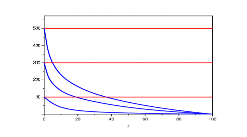
Figure 6: The singular and regularized baby skyrmion solutions which carry the $4\pi m$ magnetic flux for $m=1,2,3$. The red straight lines represent the singular solutions, and the blue curves represent the regularized solutions.

Of course, the quantization of the singular magnetic flux is topological. But the topology is not $\pi_{2}(S^{2})$ of the baby skyrmion, but $\pi_{1}(S^{1})$ of the hidden U(1). To see this notice that $\hat{n}$ of (54) defines the mapping $\pi_{1}(S^{1})$ from the $S^{1}$ circle of constant radius in the $xy$-plane to the target space $S^{1}$ of the U(1) subgroup of SU(2) which leaves $\hat{n}$ invariant ijmpa08 .

The importance of this singular solution is that the popular baby skyrmions can be viewed as the regularized magnetic vortex, regularized by the non-trivial $f(\varrho)$ which satisfies the baby skyrmion equation (48). So, just like the well known skyrmion is nothing but the regularized solution of the singular monopole (19) regularized by $\omega$, the baby skyrmion is the regularized solution of the singular vortex (54).

Actually, there is another type of totally new magnetic vortex solutions. To see this notice that

$$f(\varrho)=(2p+1)\frac{\pi}{2},~{}~{}~{}\hat{n}=\pm\left(\begin{array}[]{c}\cos{m\varphi}\\ \sin{m\varphi}\\ 0\end{array}\right),$$ (65)

also become singular solutions of (48). Clearly this describes the magnetic vortex given by the potential $C_{\mu}$,

$$C_{\mu}=-2i\xi^{\dagger}\partial_{\mu}\xi=m\partial_{\mu}\varphi,$$

$$\xi=\frac{1}{\sqrt{2}}\left(\begin{array}[]{c}1\\ e^{im\varphi}\end{array}\right),~{}~{}~{}\hat{n}=\xi^{\dagger}\vec{\sigma}\xi,$$ (68)

which has the flux

$$\Phi=\oint_{\varrho\rightarrow\infty}C_{\mu}dx^{\mu}=2\pi m.$$ (69)

This should be compared with (61).

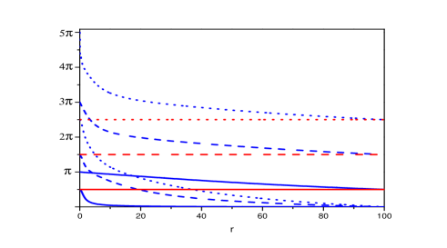
Figure 7: The singular and partly regularized baby skyrmion solutions which carry the $2\pi m$ magnetic flux for $m=1,2,3$. The red straight lines represent the singular solutions, and the blue curves represent the partly regularized solutions.

Moreover, they can also be regularized. To see this we choose the ansatz (47) and the boundary condition

$$f(0)=(2p+1)\frac{\pi}{2},~{}~{}~{}~{}f(\infty)=0.$$ (70)

With this we can solve (48) and obtain the magnetic vortex solutions described by the potential

$$C_{\mu}=-2i\xi^{\dagger}\partial_{\mu}\xi=-m\cos f\partial_{\mu}\varphi,$$

$$\xi=\left(\begin{array}[]{c}\cos\frac{f(\varrho)}{2}e^{-\frac{i}{2}m\varphi}\\ \sin\frac{f(\varrho)}{2}e^{\frac{i}{2}m\varphi}\end{array}\right),~{}~{}~{}\hat{n}=\xi^{\dagger}\vec{\sigma}\xi,$$ (73)

which has the quantized magnetic flux along the $z$-axis

$$\Phi={\displaystyle\int}H_{\varrho\varphi}d\varrho d\varphi=2\pi m.$$ (74)

Notice that, unlike (68), the magnetic potential of (73) is regular at the origin.

Furthermore, we have similar solutions with slightly different boundary condition

$$f(0)=(2p+1)\pi,~{}~{}~{}f(\infty)=(2p+1)\frac{\pi}{2}.$$ (75)

and

$$C_{\mu}=-2i\xi^{\dagger}\partial_{\mu}\xi=-m(\cos f+1)\partial_{\mu}\varphi,$$

$$\xi=\left(\begin{array}[]{c}\cos\frac{f(\varrho)}{2}e^{-im\varphi}\\ \sin\frac{f(\varrho)}{2}\end{array}\right),~{}~{}~{}\hat{n}=\xi^{\dagger}\vec{\sigma}\xi.$$ (78)

Again notice that the magnetic potential of these solutions is regular at the origin, and generates $2\pi m$ flux. These solutions for $p=0,1,2$ are shown in Fig. 7.

The energy functional of these solutions is given by

$$E=2\pi\int\mathcal{E}\varrho d\varrho=\pi\mu^{2}\int_{0}^{\infty}\Big{[}\Big{(}1+\frac{\alpha^{2}}{\mu^{2}}\frac{n^{2}}{\varrho^{2}}\sin^{2}f\Big{)}\dot{f}^{2}$$

$$+\frac{n^{2}}{\varrho^{2}}\sin^{2}f\Big{]}\varrho d\varrho.$$ (79)

So the energy density of the solution (73) is divergent at the orgin, but that of the solution (78) is divergent at the infinity. In this sense both of them are singular.

Notice, however, combining these two solutions with the boundary condition (49) we obtain the well known regular baby skyrmions. This is identical to the observation that the skyrmions are the sum of two half-skyrmions ijmpa08 . This is schematically shown in Fig. 8. The similarity between this figure and. Fig 1 is unmistakable.

Obviously the new solutions have interesting features. But the important lesson that we learn from the above exercise for our purpose in this paper is that the solution (68) is the crux, the building block, of the baby skyrmions. All other solutions stem from this. This point becomes important for us to prove the fact that the baby skyrmion can indeed be generalized to carry two topological numbers.

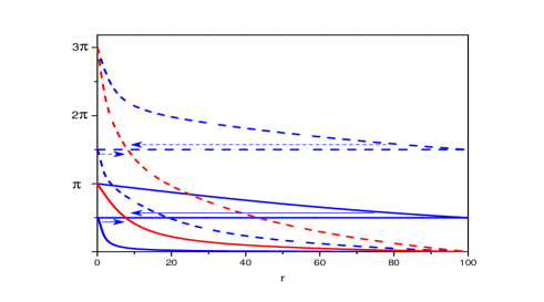
Figure 8: The regularized baby skyrmion solution with $4\pi m$ flux made of two singular baby skyrmions with $2\pi m$ flux. Here we show only $m=1,2$ solutions for simplicity.

To do that, notice first that the baby skyrmions are described by $\hat{n}$, without $\omega$. And they carry only one topological number (the quantized magnetic flux) determined by $\hat{n}$. So, by activating $\omega$, we could obtain the generalized baby skyrmions which have two topological numbers. To show that this is possible, we activate $\omega$ and generalize the ansatz (47) to

$$\omega=\omega(\varrho),~{}~{}~{}\hat{n}=\left(\begin{array}[]{c}\sin{f(\varrho)}\cos{n\varphi}\\ \sin{f(\varrho)}\sin{n\varphi}\\ \cos{f(\varrho)}\end{array}\right).$$ (83)

With this the skyrme equation (11) is reduced to

$$\Big{(}1+\frac{\alpha}{\kappa^{2}}\frac{n^{2}}{\varrho^{2}}\sin^{2}f\sin^{2}\frac{w}{2}\Big{)}\ddot{f}$$

$$+\Big{[}\frac{1}{\varrho}+\frac{\alpha}{\kappa^{2}}\frac{n^{2}}{2\varrho^{2}}\dot{f}\sin 2f\sin^{2}\frac{w}{2}-\frac{\alpha}{\kappa^{2}}\frac{n^{2}}{\varrho^{3}}\sin^{2}f\sin^{2}\frac{w}{2}$$

$$+\Big{(}\cot\frac{w}{2}+\frac{\alpha}{\kappa^{2}}\frac{n^{2}}{\varrho^{2}}\sin^{2}f\sin w\Big{)}\dot{w}\Big{]}\dot{f}$$

$$-\Big{(}\frac{n^{2}}{\varrho^{2}}+\frac{\alpha}{\kappa^{2}}\frac{n^{2}}{4\varrho^{2}}\dot{w}^{2}\Big{)}\sin f\cos f=0,$$

$$\Big{(}1+\frac{\alpha}{\kappa^{2}}\frac{n^{2}}{\varrho^{2}}\sin^{2}f\sin^{2}\frac{w}{2}\Big{)}\ddot{w}$$

$$+\Big{(}\frac{1}{\varrho}+\frac{\alpha}{\kappa^{2}}\frac{n^{2}}{\varrho^{2}}\dot{f}\sin 2f\sin^{2}\frac{w}{2}-\frac{\alpha}{\kappa^{2}}\frac{n^{2}}{\varrho^{3}}\sin^{2}f\sin^{2}\frac{w}{2}$$

$$+\frac{\alpha}{\kappa^{2}}\frac{n^{2}}{4\varrho^{2}}\dot{w}\sin^{2}f\sin w\Big{)}\dot{w}$$

$$-\Big{[}\Big{(}1+\frac{\alpha}{\kappa^{2}}\frac{2n^{2}}{\varrho^{2}}\sin^{2}f\sin^{2}\frac{w}{2}\Big{)}\dot{f}^{2}$$

$$-\frac{n^{2}}{\varrho^{2}}\sin^{2}f\Big{]}\sin w=0.$$ (84)

This is the generalized baby skyrmion equation in Skyrme theory. Notice that, when $w(\varrho)=(2p+1)\pi$, the first equation becomes exactly the baby skrymion equation (48).

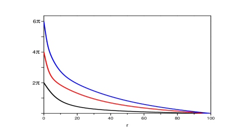
Figure 9: The generalized baby skyrmion solutions which have two topological numbers $(m,n)$. Here $f$ is fixed ($f=(2p+1)\pi/2$), and we show the solutions for $\omega$ for $n=1,2,3$.

This equation has a new set of vortex solutions. To see this, let $f(\varrho)=(2p+1)\pi/2$ as we did in (68). With this, the first equation of (84) is automatically satisfied, and the second equation becomes

$$\Big{(}1+\frac{\alpha}{\kappa^{2}}\frac{n^{2}}{\varrho^{2}}\sin^{2}\frac{w}{2}\Big{)}\ddot{w}$$

$$+\frac{1}{\varrho}\Big{(}1+\frac{\alpha}{\kappa^{2}}\frac{n^{2}}{4\varrho}\dot{w}\sin w-\frac{\alpha}{\kappa^{2}}\frac{n^{2}}{\varrho^{2}}\sin^{2}\frac{w}{2}\Big{)}\dot{w}$$

$$-\frac{n^{2}}{\varrho^{2}}\sin w=0.$$ (85)

Remarkably, this equation becomes exactly the baby skyrmion equation (48), if we identify $w(\varrho)=2f(\varrho)$. So, solving this with the boundary condition

$$\omega(0)=2\pi n,~{}~{}~{}~{}~{}\omega(\infty)=0,$$ (86)

we obtain the new generalized skyrmion solutions shown in Fig. 9.

Clearly they have singular $2\pi m$ magnetic flux, and have the energy

$$E=\frac{\pi}{4}\mu^{2}\int_{0}^{\infty}\Big{[}\Big{(}1+\frac{\alpha^{2}}{\mu^{2}}\frac{n^{2}}{\varrho^{2}}\sin^{2}\frac{w}{2}\Big{)}\dot{w}^{2}$$

$$+4\frac{n^{2}}{\varrho^{2}}\sin^{2}\frac{w}{2}\Big{]}\varrho d\varrho.$$ (87)

This tells that, unlike the singular baby skymion solution shown in (68), this solution becomes regular everywhere.

Notice that asymptotically the baby skyrmion equation (48) can be approximated to

$$\ddot{f}+\frac{1}{\varrho}\dot{f}-\frac{m^{2}}{\varrho^{2}}f\simeq 0,$$ (88)

so that the solutions shown in Figs. 6, 7, 8 (and Fig. 9) have long $1/\varrho^{m}$ (or $1/\varrho^{n}$) tails, with no exponential damping. But this is a generic feature of the baby skyrmion ijmpa08 ; piet .

These solutions are interesting because they are new. But what is really important about these baby skyrmion solutions for our purpose here is that they have two independent topology, the flux topology $\pi_{1}(S^{1})$ fixed by the invariant subgroup of $\hat{n}$ and the shell (radial) topology $\pi_{1}(S^{1})$ fixed by $\omega$.

This means that the baby skyrmions can also be generalized to carry two topological numbers, the monopole number $m$ of the magnetic flux fixed by $\hat{n}$ and the winding number $n$ of the radial excitation $n$ fixed by $\omega$. This confirms that the baby skyrmions (as well as the skyrmions) have two topology, and thus should be classified by two topological numbers.

VI Multiple Vacua of Skyrme Theory

Skyrme theory has been known to have rich topological structures. It has the Wu-Yang type monopoles which have the $\pi_{2}(S^{2})$ topology, the skyrmions which have the $\pi_{3}(S^{3})$ topology, the baby skyrmions which have the $\pi_{1}(S^{1})$ topology, and the Faddeev-Niemi knots which have the $\pi_{3}(S^{2})$ topology prl01 ; plb04 ; ijmpa08 . In the above we have shown that the theory has more topological structure, and proved that the skyrmions can be generalized to have two topological quantum numbers.

Now we show that the Skyrme theory in fact has another very important topological structure, the topologically different multiple vacua. To see this, notice that (11) has the solution

$$\omega=2\pi p,~{}~{}~{}(p;~{}integer),$$ (89)

independent of $\hat{n}$. And obviously this is the vacuum solution.

This tells that the Skyrme theory has multiple vacua classified by the integer $p$ which is similar to the Sine-Gordon theory. But unlike the Sine-Gordon theory, here we have the multiple vacua without any potential. Moreover, the above discussion tells that the spherically symmetric skyrmions connect and occupy the $p+1$ adjacent vacua. This means that we can connect all vacua with the spherically symmetric skyrmions. Of course, one could introduce such vacua in Skyrme theory introducing a potential term in the Lagrangian nitta . This is not what we are doing here. We have these vacua without any potential.

But this is not the end of the story. To see this notice that (89) becomes the vacuum independent of $\hat{n}$. This means that $\hat{n}$ can add the $\pi_{3}(S^{2})$ topology to each of the multiple vacua classified by another integer $q$, because it is completely arbitrary. And this is precisely the knot topology of the QCD vacuum plb07 .

Actually this is not be surprising. As we have already emphasized, there is a deep connection between Skyrme theory and QCD. So it is natural that the Skyrme theory and QCD have similar vacuum structure. To clarify this point we introduce a right-handed unit isotriplet $(\hat{n}_{1},\hat{n}_{2},\hat{n}_{3}=\hat{n})$, and impose the vacuum isometry to the SU(2) gauge potential,

$${}^{\forall_{i}}D_{\mu}\hat{n}_{i}=0,$$ (90)

which assures $\vec{F}_{\mu\nu}=0$. From this we obtain the most general SU(2) QCD vacuum potential plb07

$${\vec{A}}_{\mu}\rightarrow\hat{\Omega}_{\mu}=-\dfrac{1}{2}\epsilon_{ijk}(\hat{n}_{i}\cdot\partial_{\mu}\hat{n}_{j})~{}\hat{n}_{k}$$

$$=\dfrac{1}{2}\epsilon_{ijk}(\hat{n}_{i}\cdot\partial_{\mu}\hat{n}_{j})~{}\hat{e}_{k},$$ (91)

where $\hat{e}_{1}=(1,0,0),\hat{e}_{2}=(0,1,0),\hat{e}_{3}=(0,0,1)$.

This is the QCD vacuum which has the knot topology $\pi_{3}(S^{3})\simeq\pi_{3}(S^{2})$. It is clear that (91) describes the $\pi_{3}(S^{3})$ topology, since $(\hat{n}_{1},\hat{n}_{2},\hat{n})$ defines the mapping $\pi_{3}(S^{3})$ from the compactified 3-dimensional space to the SU(2) group space. But notice that $(\hat{n}_{1},\hat{n}_{2},\hat{n})$ is completely determined by $\hat{n}$, up to the U(1) rotation which leaves $\hat{n}$ invariant, which describes the mapping from the real space $S^{3}$ to the coset space $S^{2}$ of $SU(2)/U(1)$. So the QCD vacuum (91) can also be classified by the knot topology $\pi_{3}(S^{2})$ plb07 .

Now it must be clear why the Skyrme theory has the same knot topology. As we have noticed, the Skyrme theory has the vacuum (89), independent of $\hat{n}$. But this $\hat{n}$ (just as in the SU(2) QCD) defines the mapping $\pi_{3}(S^{2})$, with the $S^{3}$ compactification of $R^{3}$, and thus can be classified by the knot topology. Of course, in the Skyrme theory we do not need the vacuum potential (91) to describe the vacuum. We only need $\hat{n}$ which describes the knot topology.

This tells that the vacuum in Skyrme theory has the topology of the Sine-Gordon theory and QCD combined together. This means that the vacuum of the Skyrme theory can also be classified by two quantum numbers $(p,q)$, the $\pi_{1}(S^{1})$ of $\omega$ and $\pi_{3}(S^{2})$ of $\hat{n}$. And this is so without any extra potential. As far as we know, there is no other theory which has this type of vacuum topology.

At this point we emphasize the followings. First, the knot topology of $\hat{n}$ is different from the monopole topology of $\hat{n}$. The monopole topology $\pi_{2}(S^{2})$ is associated to the isolated singularities of $\hat{n}$, but the knot topology $\pi_{3}(S^{2})$ does not require any singularity for $\hat{n}$. And for a classical vacuum $\hat{n}$ must be completely regular everywhere. So only the knot topology, not the monopole topology, can not describe a classical vacuum. And this is precisely the vacuum topology of QCD.

Second, the knot topology of the vacuum is different from the Faddeev-Niemi knot that we have in the Skyrme theory prl01 . The Faddeev-Niemi knot is a unique and real (i.e., physical) knot which carries energy, which is given by the solution of (13). In particular, we have the knot solution when $\omega=(2n+1)\pi$. On the other hand, we have the knot of the vacuum when $\omega=2\pi p$. Moreover, the vacuum knot has no energy, and is not unique. While the Faddeev-Niemi knot is unique, there are infinitely many $\hat{n}$ which describes the same vacuum knot topology. So obviously they are different.

What is really remarkable is that the same $\hat{n}$ has multiple roles. It describes the monopole topology, the knot topology of Faddeev-Niemi knot, and the knot topology of the vacuum.

The fact that the Skyrme theory has topologically distinct vacua raises more questions. Do we have the vacuum tunneling in Skyrme theory? If so, what instanton do we have in this theory? How different is it from the QCD instanton?

VII Discussions

The Skyrme theory was proposed as a low energy effective theory of strong interaction where the baryons appear as the topological solitons made of pions, the Nambu-Goldstone field of the chiral symmetry breaking sky ; witt ; rho . This view has become the standard view man ; bat ; houg .

But the Skyrme theory has many faces. As we have pointed out, the theory can actually be viewed as a theory of monopole which has the built-in Meissner effect prl01 ; plb04 ; ijmpa08 . In fact all classical objects in Skyrme theory stem from the monopole. Of course, the fact that the skyrmion is closely related to the monopole has been well known. The rational map $\pi_{2}(S^{2})$ of $\hat{n}$ which determines the baryon number in the popular non spherically symmetric skyrmions has been associated to the monopole topology from the beginning man ; bat ; houg . But so far the fact that the skyrmion itself becomes the monopole has not been widely appreciated.

In this paper we have shown that the skyrmions are not just the dressed monopoles but actually carry the monopole number, so that they can be classified by two topological numbers, the baryon number and the monopole number. Moreover, we have shown that here the baryon number could be replaced by the radial (shell) number, so that the skyrmions can be classified by two topological numbers $(m,n)$, the monopole number $m$ which describes the $\pi_{2}(S^{2})$ topology of the $\hat{n}$ field and the radial (shell) number $n$ which describes the $\pi_{1}(S^{1})$ topology of the $\omega$ field. In this scheme the baryon number $B$ is given by the product of two integers $B=mn$. This comes from the following facts. First, the SU(2) space $S^{3}$ admits the Hopf fibering $S^{3}\simeq S^{2}\times S^{1}$. Second, the Skyrme theory has two variables, the angular variable $\omega$ which can represent the $\pi_{1}(S^{1})$ topology and the coset variable $\hat{n}$ which represents the $\pi_{2}(S^{2})$ topology.

In this view the popular (non spherically symmetric) skyrmions are classified as the $(m,1)$ skyrmions, and the radially excited spherically symmetric skyrmions are classified as the $(1,n)$ skyrmions. and we can construct the $(m,n)$ skyrmions adding the shell structure to the $(m,1)$ skyrmions. Moreover, we have shown that the skyrmions, when they are generalized to have two topological numbers, should have the topological stability of the two topology independently.

Furthermore, we have shown that the baby skyrmions can also be generalized to carry two topology. Reactivating the radial variable $\omega$, we have shown that the baby skyrmions in Skyrme-Faddeev theory can be generalized to new baby skyrmions in Skyrme theory. And this generalization naturally introduces a new $\pi_{1}(S^{1})$ topology to the generalized solutions. This means that the new generalized baby skyrmions carry two topology, the shell (radial) topology$\pi_{1}(S^{1})$ of $\omega$ and the monopole topology $\pi_{2}(S^{2})$ of $\hat{n}$, and thus are classified by two topological numbers. This is remarkable.

As importantly, we have shown that the Skyrme theory has multiple vacua. The vacuum of the theory has the structure of the vacuum of the Sine-Gordon theory and at the same time the structure of QCD vacuum. So the vacuum can also be classified by two topological numbers $p$ and $q$ which represent the $\pi_{1}(S^{1})$ topology of the $\omega$ field and the $\pi_{3}(S^{2})$ topology of the $\hat{n}$ field.

The fact that the vacuum of the Skyrme theory has the $\pi_{1}(S^{1})$ topology is not surprising, considering that it has the angular variable $\omega$. Moreover, the fact that the vacuum of the Skyrme theory has the $\pi_{3}(S^{2})$ topology of the QCD vacuum could easily be understood once we understand that the Skyrme theory is closely related to QCD. What is really remarkable is that it has both $\pi_{1}(S^{1})$ and $\pi_{3}(S^{2})$ topology at the same time. As far as we understand there is no other theory which has this feature. This again is closely related to the fact that $S^{3}$ admits the Hofp fibering and that the theory has two variables $\omega$ and $\hat{n}$.

As we have remarked, our results raises more questions. Can we extend the Faddeev-Niemi knots activating $\omega$ to have the shell structure? How can we obtain such solutions? How about the vacuum tunneling in Skyrme theory? What instanton do we have in this theory? The questions continue.

Clearly the above observations put the Skyrme theory in a totally new perspective. Our results in this paper show that the theory has so many new aspects which make the theory more interesting. But most importantly our results put the popular interpretation of the Skyrme theory in an awkward position, and strongly imply that we need a new interpretation of the Skyrme theory.

First of all, our result tells that the skyrmions carry two topological numbers which are conserved independently. So, if the skyrmions become the baryons, the baryons must have two conserved quantities. This is very difficult to accommodate, because the baryons seem to have no conserved quantity other than the baryon number.

Moreover, the Skyrme theory have the (generalized) baby skyrmions which can be viewed as skyrmion-antiskyrmion pair infinitely separated apart. So, if the skyrmions become the baryons, we must have the string-like hadrons. In fact, the theory has too many topological solitons which could be interpreted as strongly interacting particles. It has not only the skyrmions but also the Faddeev-Niemi knots. In this case the knots should be interpreted as mesons made of baryon-antibaryon pair.

But the knots are expected to have huge mass, roughly about 10 times heavier than the proton mass, simply because of the geometricshape plb04 ; ijmpa08 . So, if the skyrmion is treated as the baryon, we must accept the existence of a topologically stable meson 10 times heavier than proton. And we should take this possibility seriously.

All of these evidences strongly suggest that the Skyrme theory need a totally new interpretation. It simply has too many interesting featutres to be considered as a theory of strong interaction. These new features and the questions raised in this paper will be discussed in a separate publication cho .

ACKNOWLEDGEMENT

The work is supported in part by the National Natural Science Foundation of China (Grant 11575254), Chinese Academy of Sciences Visiting Professorship for Senior International Scientists (Grant 2013T2J0010), Chinese Scholarship Council, National Research Foundation of Korea funded by the Ministry of Education (Grants 2015-R1D1A1A0-1057578 and 2015-R1D1A1A0-1059407), and by Konkuk University.

References

- (1) T.H.R. Skyrme, Proc. Roy. Soc. (London) 260, 127 (1961); 262, 237 (1961); Nucl. Phys. 31, 556 (1962).
- (2) G. Adkins, C. Nappi, and E. Witten, Nucl. Phys. B228, 552 (1983).
- (3) A. Jackson and M. Rho, Phys. Rev. Lett. 51, 751 (1983).
- (4) E.B. Bogomol’ny and V.A. Fateev, Soy. J. Nucl. Phys. 37, 134 (1983).
- (5) See, for example, I. Zahed and G. Brown, Phys. Rep. 142, 1 (1986).
- (6) N.S. Manton, Phys. Lett. B192, 177 (1987).
- (7) R.A. Battye and P.M. Sutcliffe, Phys. Rev. Lett. 79, 363 (1997).
- (8) C.J. Houghton, N.S. Manton, and P.M. Sutcliffe, Nucl. Phys. B510,507 (1998).
- (9) R.A. Battye and P.M. Sutcliffe, Phys. Rev. Lett. 86, 3989 (2001); Rev. Math. Phys. 14, 29 (2002).
- (10) N.S. Manton and B. Piette, in Proceedings of the European Congress of Mathematics, Barcelona (2000), edited by C. Casacuberta et al., Progress in Mathematics Vol. 201 (Birkhauser, Basel, 2001).
- (11) B. Piette and G. Probert, Phys. Rev. D75, 125023 (2007).
- (12) D.T.J. Feist, P.H.C. Lau, N.S. Manton, Phys. Rev. D87, 085034 (2013).
- (13) F. Hoyle, Astrophys. J. Suppl. 1, 121 (1954).
- (14) E. Epelbaum, H. Krebs, D. Lee, and U. Meissner, Phys. Rev. Lett. 106, 192501 (2011).
- (15) P.H.C. Lau and N.S. Manton, Phys. Rev. Lett. 113, 232503 (2014).
- (16) C.J. Halcrow and N.S. Manton, JHEP 1501, 016 (2015).
- (17) C. Adam, J. Sanches-Guillen, and A. Wereszczynski, Phys. Lett B691,105 (2010); Phys. Rev. Lett. 111, 232501 (2013).
- (18) Y.M. Cho, Phys. Rev. Lett. 87, 252001 (2001).
- (19) Y.M. Cho, Phys. Lett. B603, 88 (2004).
- (20) Y.M. Cho, B.S. Park, and P.M. Zhang, Int. J. Mod. Phys. A23, 267 (2008).
- (21) J. Ruostekoski and J.R. Anglin, Phys. Rev. Lett. 86, 3934 (2001); R.A. Battye, N.R. Cooper, and P.M. Sutcliffe, Phys. Rev. Lett. 88, 080401 (2002).
- (22) O.V. Manko, N.S. Manton, and S.W. Wood, Phys. Rev. C76, 055203 (2007).
- (23) Y.M. Cho, Hyojoong Khim, and Pengming Zhang, Phys. Rev. A72, 063603 (2005); Y.M. Cho and P.M. Zhang, Euro. Phys. J. B65, 155 (2008).
- (24) Y.M. Cho, Kyoungtae Kimm, J.H. Yoon, and Pengming Zhang, Euro Phys. J. C 77, 88 (2017).
- (25) Y.M. Cho, Phys. Rev. D21, 1080 (1980). See also Y.S. Duan and M.L. Ge, Sci. Sinica 11,1072 (1979).
- (26) Y.M. Cho, Phys. Rev. Lett. 46, 302 (1981); Phys. Rev. D23, 2415 (1981).
- (27) Y.M. Cho, Phys. Rev. Lett. 44, 1115 (1980).
- (28) F. Canfora and G. Tallarita, Phys. Rev. D91, 085033 (2015); D94, 025037 (2016).
- (29) B. Piette, B. Schroers, and W. Zakrzewski, Nucl. Phys. 439, 205 (1995).
- (30) S.B. Gudnason and M. Nitta, Phys. Rev. D90, 085007 (2014).
- (31) Y.M. Cho, Phys. Lett. B644, 208 (2007).
- (32) Liping Zou, B.S. Park, Pengming Zhang, and Y.M. Cho, to be published.