Clustering of galaxies around AGN in the HSC Wide survey

Abstract

We have measured the clustering of galaxies around active galactic nuclei (AGN) for which single-epoch virial masses of the super-massive black hole (SMBH) are available to investigate the relation between the large scale environment of AGNs and the evolution of SMBHs. The AGN samples used in this work were derived from the Sloan Digital Sky Survey (SDSS) observations and the galaxy samples were from 240 deg${}^{2}$ S15b data of the Hyper Suprime-Cam Subaru Strategic Program (HSC-SSP). The investigated redshift range is 0.6–3.0, and the masses of the SMBHs lie in the range $10^{7.5}$–$10^{10}$ M${}_{\solar}$. The absolute magnitude of the galaxy samples reaches to $M_{\lambda 310}$ $\sim$ $-$18 at rest frame wavelength 310 nm for the low-redshift end of the samples. More than 70% of the galaxies in the analysis are blue. We found a significant dependence of the cross-correlation length on redshift, which primarily reflects the brightness dependence of the galaxy clustering. At the lowest redshifts the cross-correlation length increases from 7 $h^{-1}$ Mpc around $M_{\lambda 310}$ $=$ $-19$ mag to $>$10 $h^{-1}$ Mpc beyond $M_{\lambda 310}$ $=$ $-20$ mag. No significant dependence of the cross-correlation length on BH mass was found for whole galaxy samples dominated by blue galaxies, while there was an indication of BH mass dependence in the cross-correlation with red galaxies. These results provides a picture of the environment of AGNs studied in this paper being enriched with blue starforming galaxies, and a fraction of the galaxies are being evolved to red galaxies along with the evolution of SMBHs in that system.

1 Introduction

Most galaxies have a supermassive black hole (SMBH) with mass greater than $\sim$10${}^{6}$ M${}_{\solar}$ at their center (Richstone+98). Observations of the local Universe have revealed that the mass of the SMBH correlates with the several properties of the bulge component of the host galaxy (Magorrian+98; Ferrarese+00; Gebhardt+00; Ho-07). This observational evidence suggests that a SMBH and its host galaxy co-evolve in a coordinated way in spite of the nine orders of difference in their physical size scale (Kormendy+13).

SMBHs grow through the accretion of gas from their host galaxies or large-scale environment. Accretion in a secular mode, which arises through internal dynamical processes such as bar or disk instability or external processes driven by galaxy interaction, is one of the mechanisms to deliver the gas into the SMBH (Kormendy+04). As the mass accretion rate of the secular mode cannot be as high as to maintain the activity seen in bright QSOs (Menci+14), this mode could operate in lower-luminosity AGNs.

A merger of galaxies can induce gravitational torques which drive inflows of cold gas toward the center of galaxies (e.g., Hopkins+08). Observational evidence has been obtained that shows the relation between AGN activity and a galaxy merger (e.g., Sanders+88; Treister+12). The activity of the bright QSOs could be explained by this model. Although the accretion can be the most efficient in this mode, it is also expected that AGN feedback promptly operates and stops the gas inflows when the mass of the SMBH becomes as large as 10${}^{9}$ M${}_{\solar}$ (Fanidakis+13).

As an alternative process to make a SMBH evolve above 10${}^{9}$ M${}_{\solar}$, quiescent gas accretion from the hot halo (Keres+09; Fanidakis+13) and/or recycled gas from evolving stars (Ciotti+01; Ciotti+07) has been proposed. According to the predictions of semi-analytical modeling by Fanidakis+13, AGNs fueled in the hot-halo mode are located in more massive dark matter haloes than the AGNs fueled in the merger-driven starburst mode.

The mass of the host dark matter halo that AGNs reside can be inferred from the auto-correlation function of AGNs at distance scale $>$1 Mpc. According to the analysis of auto-correlation of SDSS QSOs by Ross+09, the halo mass is almost constant at $\sim$2$\times 10^{12}h^{-1}M_{\solar}$ in the redshift range from 0.3 to 2.2. It is also possible to estimate the halo mass from the cross-correlation between AGNs and galaxies if the auto-correlation functions of galaxies are precisely obtained. According to the cross-correlation studies the dark matter halo mass estimated to be $10^{12}$–$10^{13.5}h^{-1}M_{\solar}$ depending on the detection wavelength of the AGNs (e.g. Hickox+09; Krumpe+12). Studies on clustering and/or environments of AGNs have also been reported elsewhere (e.g. Croom+05; Coil+09; Silverman+09; Donoso+10; Allevato+11; Bradshaw+11; Shen+13; Mountrichas+13; Zhang+13; Georgakakis+14; Krumpe+15; Ikeda+15).

In spite of a large number of AGN clustering studies published so far, the studies focused on the relation between the mass of the central BH, which is the most fundamental property on which the history of mass accretion is imprinted, and also the properties of galaxies such as color and luminosity function around it are very limited. Since the interaction in the scale of group or cluster of galaxies can induce concurrent activities of starformation, mass accretion to the central BH, and transition to the red sequence in the constituent galaxies, the contribution of such large-scale phenomena to the evolution of SMBH can be inferred from the surrounding galaxies.

Shen+09 measured the clustering of QSOs for samples divided by their BH mass at redshifts 0.4–2.5 and didn’t find significant dependence except for the most massive sample for which marginally larger clustering was found in $\sim$2$\sigma$ level. Komiya+13 examined dependence of the AGN-galaxy clustering on the BH mass at redshift range from 0.3 to 1.0 using the UKIDSS data for the galaxy samples, and found that the cross-correlation length increases above $10^{8.2}M_{\solar}$. Krolewski+15 also examined the BH mass dependence of the AGN-galaxy clustering at redshift $\sim$0.8 using SDSS and WISE data for the galaxy samples, and found no significant relationship between clustering amplitude and BH mass. Krumpe+15 measured clustering of soft X-ray and optically selected AGNs at redshifts from 0.16 to 0.36 and detected a weak dependence on the mass at significance level of 2.7 $\sigma$, while they didn’t detect significant dependence on the Eddington ratio. They conclude that the mass dependence is the origin of the observed weak X-ray luminosity clustering dependence.

Extending the dataset of Komiya+13, Shirasaki+16 derived, for the first time as derived from statistically significant number of samples, color and absolute magnitude distributions of galaxies around AGNs, and found that the increase of the cross-correlation length found by Komiya+13 is due to the increase in the number density of red galaxies. Those results indicate that the most massive SMBHs are evolved in dark matter haloes more massive than the lower mass SMBHs, and the surrounding galaxies also evolve in a coordinated way with the SMBHs which are mostly located in the center of host halo. To extend further the study given in Shirasaki+16 up to redshifts $\sim$3, which covers the era of the peak of star formation and mass accretion rate to SMBHs, we require a deeper wide multi-band survey.

The Hyper Suprime-Cam Subaru Strategic Program (HSC-SSP) is a multi-band imaging survey conducted with the HSC on the 8.2m Subaru Telescope. The survey consists of three layers: Wide (1400 deg${}^{2}$, r $\sim$26), Deep (27 deg${}^{2}$, r$\sim$27), and UltraDeep (3.5 deg${}^{2}$, r$\sim$28). The HSC-SSP Wide survey provides the first opportunity to investigate the environment of AGNs up to redshift three with unprecedented statistics. Using the unique dataset of HSC-SSP Wide survey, this paper’s purpose is to measure not only the clustering of galaxies around AGNs but also their color and luminosity distribution as a function of SMBH mass at five redshift groups from 0.6 to 3.0. The results obtained in this work would give us a unified picture of evolution of galaxies and SMBHs under the large-scale structure of the Universe at their most important stage.

Throughout this paper, we assume a cosmology with $\Omega_{m}=0.3$, $\Omega_{\lambda}=0.7$, $h=0.7$ and $\sigma_{8}=0.8$. All magnitudes are given in the AB system. All the distances are measured in comoving coordinates. The correlation length is presented in unit of $h^{-1}$Mpc. The group and parameter names that are frequently refereed to in the text are summarized in Table LABEL:tab:param_desc of the Appendix.

2 Datasets

2.1 AGNs

The AGN samples used in this paper were drawn from the QSO properties catalog of Shen+11 (S11) and SDSS DR12 Quasar catalog (DR12Q) of Paris+17. We used S11 catalog as a reference for the black hole (BH) mass estimate to be consistent with the previous studies (Komiya+13; Shirasaki+16), and the BH masses derived from the DR12Q catalog and spectral measurements were calibrated with those derived in S11.

We divided the AGN samples according to their measured redshift and BH mass. The mass used in this analysis is based on the H$\beta$, Mg II, or C IV line width as given in the S11 and DR12Q catalogs. For AGNs drawn from the DR12Q catalog, the mass was calculated according to the formula derived by Mejia-Restrepo+16 as follows:

$$M_{\rm BH,MgII}=8.05\times 10^{6}~{}M_{\solar}\left(\frac{L_{\lambda 300}}{10^{44}~{}{\rm erg~{}s^{-1}}}\right)^{0.609}\left(\frac{\rm FWHM(Mg~{}II)}{\rm km~{}s^{-1}}\right)^{2},$$ (1)

$$M_{\rm BH,CIV}=5.71\times 10^{5}~{}M_{\solar}\left(\frac{L_{\lambda 145}}{10^{44}~{}{\rm erg~{}s^{-1}}}\right)^{0.57}\left(\frac{\rm FWHM(C~{}IV)}{\rm km~{}s^{-1}}\right)^{2}\left(\frac{L_{\rm p}(\rm C~{}III])}{L_{\rm p}(\rm C~{}IV)}\right)^{-2.09},$$ (2)

where $L_{\lambda 300}$ and $L_{\lambda 145}$ are the continuum luminosity at 300 nm and 145 nm respectively, FWHM(Mg II) and FWHM(C IV) are the full width at half-maximum of the Mg II and C IV emission lines respectively, and $L_{p}(\rm C~{}III])$ and $L_{p}(\rm C~{}IV)$ are peak luminosities of the corresponding lines. We measured the continuum luminosities, $L_{\lambda 300}$ and $L_{\lambda 145}$, and the luminosity ratio, $\frac{L_{\rm p}(\rm C~{}III])}{L_{\rm p}(\rm C~{}IV)}$ directly from the SDSS spectra, while the FWHMs of the emission lines were taken from the DR12Q catalog.

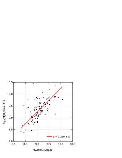
Figure 1: Comparisons of BH masses derived by different methods for the same object. Left panel shows the comparison between the BH masses as given in S11 (Shen+11) and those calculated for the same object in DR12Q (Paris+17) using equation (1). Right panel shows the comparison between the BH masses calculated for an object in DR12Q using equation (1) and (2). The solid lines represent linear expressions fitted to the data points.

To check the consistency between the BH masses derived by different relations, we compared them for the same objects. The left panel in Figure 1 shows the comparison of black hole masses given in S11, M${}_{\rm BH,MgII}$(S11), and those calculated for the same object in DR12Q, M${}_{\rm BH,MgII}$(DR12Q), using equation (1). We found there is a systematic offset of 0.24 dex and scatter of 0.22, so we have corrected for the offset to the mass calculated using equation (1).

The right panel in Figure 1 shows the comparison of black hole masses calculated for objects in DR12Q using equation (1), M${}_{\rm BH,MgII}$(DR12Q), and equation (2), M${}_{\rm BH,CIV}$(DR12Q). Systematic offset of 0.07 dex and scatter of 0.48 dex were found between them. Thus the offset of M${}_{\rm BH,CIV}$(DR12Q) to M${}_{\rm BH,MgII}$(S11) was estimated to be 0.17, and the corresponding correction was made to M${}_{\rm BH,CIV}$(DR12Q). As mentioned in Mejia-Restrepo+16 and apparent from Figure 1, M${}_{\rm BH,CIV}$ has a larger uncertainty than the mass measured based on other emission lines, so we used M${}_{\rm BH,MgII}$, whenever it was available, as a mass estimator in first priority. The AGN samples given the C IV BH mass are mostly at $z\geq 2.3$. The effect of the large uncertainty of the C IV BH mass is limited only to the results for $z\geq 2.0$.

Coatman+16 recently showed that an empirical correction to C IV BH masses based on the blueshift of C IV emission line reduces the uncertainty. To apply the correction requires an accurate measure of the AGN systemic redshift. Thus, we decided to use the relation of equation (2) which does not require precise spectroscopic measurements.

The systematic offset and scatter between $M_{\rm BH,H\beta}$ and $M_{\rm BH,Mg~{}II}$ given in S11 catalog are 0.009 dex and 0.38 dex respectively as shown in Figure 10 of Shen+11. Thus, no correction to $M_{\rm BH,H\beta}$ is required.

For AGNs appearing in both catalogs, we used the redshift and black hole mass of the S11 catalog. The redshift range of the AGNs was chosen to be 0.6–3.0, so that it overlaps with the highest redshift bin ($z$=0.6–1.0) of the previous studies (Komiya+13; Shirasaki+16) to cross check between both the results and extend up to the limit of sensitivity of this analysis. The BH mass range was set to $10^{7}$–$10^{11}$M${}_{\solar}$. We selected 6166 AGNs which are in the redshift and BH mass range and are located within the footprint of HSC-SSP Wide survey.

2.2 Galaxies

The galaxy sample was collected from the Hyper Suprime-Cam Subaru Strategic Program (HSC-SSP) S15b Wide survey dataset. HSC-SSP is a three-layered, multi-band ($grizy$ plus 4 narrow-band filters) imaging survey with the Hyper Suprime-Cam (HSC) (Miyazaki+12; Miyazaki+17) on the 8.2m Subaru Telescope. The total area and the depth of observation will be 1400 deg${}^{2}$ with $r\sim 26$ (Wide layer), 27 deg${}^{2}$ with $r\sim 27$ (Deep layer), and 3.5 deg${}^{2}$ with $r\sim 28$ (UltraDeep layer).

Summary of the survey area Field name Center coordinates $S_{i}$${}^{a}$ $S_{griz}$${}^{b}$ deg${}^{2}$ deg${}^{2}$ XMM-LSS 02${}^{h}$18${}^{m}$ $-$04${}^{\circ}$30’ 51.8 48.9 GAMA09H 09${}^{h}$00${}^{m}$ $+$01${}^{\circ}$00’ 53.0 41.9 WIDE12H 11${}^{h}$58${}^{m}$ $+$00${}^{\circ}$00’ 32.5 24.6 GAMA15H 14${}^{h}$32${}^{m}$ $+$00${}^{\circ}$00’ 38.6 35.4 HECTOMAP 16${}^{h}$24${}^{m}$ $+$43${}^{\circ}$30’ 9.6 9.0 VVDS 22${}^{h}$24${}^{m}$ $+$01${}^{\circ}$00’ 52.0 47.8 AEGIS 20${}^{h}$58${}^{m}$ $+$52${}^{\circ}$30’ 1.9 1.8 ${}^{a}$ Effective area of $i$-band detected samples. ${}^{b}$ Effective area of four-band detected samples.

We used the dataset derived from Wide layer. The observed locations and effective area are summarized in Table 2.2. The typical depths of the observation are 26.8, 26.4, 26.4, 25.5, 24.7 for $g$, $r$, $i$, $z$, and $y$ bands, respectively. The detail of survey itself is described in Aihara+17a, and the content of the S15b dataset is in Aihara+17b. The S15b dataset were analyzed through the HSC pipeline (version 4.0.1) developed by the HSC software team using codes from the Large Synoptic Survey Telescope (LSST) software pipeline (Ivezic+08; Axelrod+10). The photometric and astrometric calibrations are made based on data obtained from the Panoramic Survey Telescope and Rapid Response System (Pan-STARRS) 1 imaging survey (Magnier+13; Schlafly+12; Tonry+12).

The photometric magnitude used in this work is a CModel magnitude. The galactic reddening was corrected according to the dust maps derived by Schlegel+98.

The analysis performed in this paper is based on two galaxy samples; one is the $i$-band detected sample which is drawn from all sources selected by the criteria for $i$-band as described below and measured to be brighter than 27 magnitude in $i$-band regardless of the detection in the other four bands; the other is the four-band detected sample which is selected by enforcing the same criteria for $griz$-bands except for the magnitude cut adapted only to $i$-band data, regardless of the detection in $y$-band. Since the observations in $y$-band are shallower than the others, the detection in $y$-band was not required to avoid the bias to redder galaxies. For the cross-correlation analysis, we used the $i$-band detected sample. When we measure the distribution of galaxy color and luminosity around AGNs, we used the four-band detected sample. The term ”detected” used here means that the source satisfies the criteria defined below and has a non-NULL magnitude.

The criteria used to select $i$-band detected samples are:

   iflags_pixel_edge is not True
   AND iflags_pixel_interpolated_any is not True
   AND iflags_pixel_saturated_any is not True
   AND iflags_pixel_cr_any is not True
   AND iflags_pixel_bad is not True
   AND icmodel_flux_flags is not True
   AND icentroid_sdss_flags is not True
   AND detect_is_tract_inner is True
   AND detect_is_patch_inner is True
   AND deblend_nchild = 0

where iflags_pixel_edge is true if the source is near the edge of the frame; iflags_pixel_interpolated_any is true if any pixels in the source footprint have been interpolated due to saturation or cosmic rays; iflags_pixel_saturated_any is true if any pixels are saturated; iflags_pixel_cr_any is true if any pixels are masked as cosmic rays; iflags_pixel_bad is true if any pixels are masked for non-functioning or in severely vignetted areas; icmodel_flux_flags is false if the cmodel measurement fails; icentroid_sdss_flags is false if the SDSS centroiding algorithm fails; detect_is_tract_inner and detect_is_patch_inner are true if the source is in the inner region of a tract and patch, which is used to select a source of primary detection; deblend_nchild is the number of children this source was deblended into. Similar flag checks were performed for the other bands.

In addition to the above criteria, we adapted a criterion:

    flags_pixel_bright_object_center is not True

to remove the galaxy samples in bright source masks only for those located at $\geq$2 Mpc from the AGN. The bright source masks implemented in this data release are over-conservative in the choice of radius, so it has a drawback that decreases the significance of the clustering. Thus we did not adapt the bright source mask to the galaxy samples located at $<$2 Mpc from the AGN.

We found that there is a non-negligible number of false detections in the deblended sources, especially at larger magnitudes. To remove the false detections, we selected only the deblended sources which are brighter than 27 mag in $i$-band and also brighter than $m_{i,\rm top}+6$ mag, where $m_{i,\rm top}$ is an $i$-band magnitude brightest in the deblended sources which belong to the same parent. To avoid saturation in HSC photometry, no magnitude data brighter than 20 mag were used for any of the five bands.

2.3 AGN dataset selection

In the analysis of this paper, we treated each AGN and its surrounding galaxies as a set. Hereafter, we refer to the unit of the dataset as an AGN dataset. In this section we describe the criteria to include the AGN datasets for analysis.

For each AGN dataset, we measured the surface density of galaxies in annuli spaced by 0.2 Mpc out to 10 Mpc from the position of AGN. We kept only those AGN in which $>$60% of the area of all annuli at $\geq$2 Mpc around it and $>$80% of the area at $<$2Mpc were included in the survey footprint and not masked by bright sources. By this selection, among the original 6166 AGN datasets, 346 datasets were removed for the $i$-band detected sample and 585 were removed for the four-band detected sample. Thus 5820 and 5581 AGN datasets passed this selection for $i$-band and four-band detected samples, respectively.

The spatial uniformity of the galaxy samples in the AGN field was also examined to identify the AGN datasets that are significantly contaminated by nearby galaxies and stellar groups or showing non-uniformity for any other reason. For this purpose, we calculated two parameters for the radial number density distribution of galaxies, $\chi^{2}$ and $\sigma_{\rm max}$, where $\chi^{2}$ is a square sum of the deviation from the number density distribution fitted to the observed data using equation (6), which will be derived in section 3.1, $\sigma_{\rm max}$ is a maximum deviation from the density distribution. Adapted criteria for those parameters are: $\chi^{2}/n\leq 3.0$ and $\sigma_{\rm max}\leq 5$. By this selection, 268 (236) AGN datasets were removed from the 5820 (5581) AGN datasets for the $i$-band (four-band) detected sample. Thus 5552 (5345) AGN datasets passed all the above selections.

Figure 2 shows the mass vs redshift distribution of the AGNs that were selected according to the conditions described above and used in the cross-correlation analysis in this paper. Figures 3 and 4 show histograms of redshift and black hole mass, respectively. We divided the redshift range into five groups as shown in Figure 2, which we call z0, z1, z2, z3 and z4 for $z=$ 0.6–1.0, 1.0–1.5, 1.5–2.0, 2.0–2.5, and 2.5–3.0, respectively. For each redshift group, except for z4, the BH mass range was divided into two groups M8 and M9 so that each group has a similar number of AGNs rather than being divided at the same mass. This is because the effect of sample variance becomes dominant when the number of AGN samples is small and it is difficult to homogenize the samples among different mass groups by the division at constant mass for all the redshifts. The mass group was divided at $\log{(M_{\rm BH}/M_{\solar})}$ = 8.4, 8.8, 9.0, and 8.9 for z0, z1, z2 and z4 redshift groups, respectively, which allows us to make the statistical uncertainties even for both mass groups. The mass dependence for the z4 redshift group was not examined, since the number of samples in the z4 group is too small to do so.

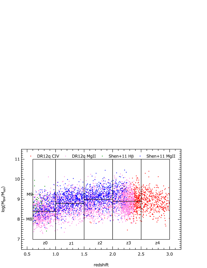
Figure 2: Distribution of redshift and BH mass of 5552 AGNs which are used in cross-correlation analysis using $i$-band detected galaxy samples.

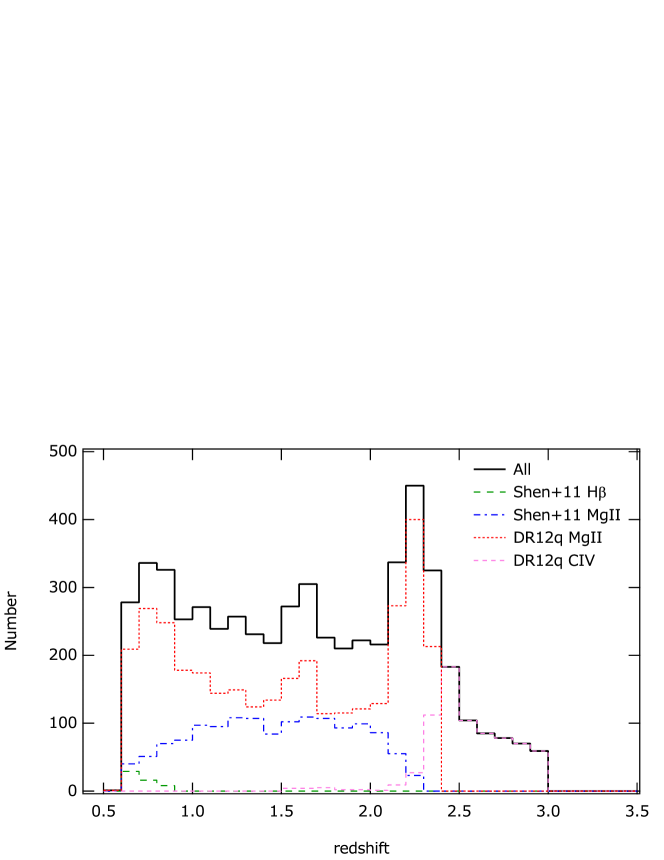
Figure 3: Distribution of BH mass for the samples shown in Figure 2.

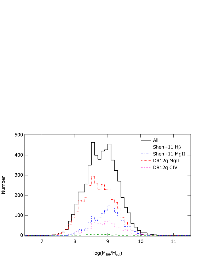
Figure 4: Distribution of redshift for the samples shown in Figure 2.

Table 2.3 shows the number of AGN datasets which passed all the selection criteria described above for each dataset. The $i$-band detected galaxy samples were used for cross-correlation analysis, and the four-band detected samples were used for deriving color distribution and luminosity function of clustering galaxies, and they were also used to measure the dependence of cross-correlation length on galaxy luminosity. The redshift-matched samples were used for examining the BH mass dependence at each redshift.

Number of AGN samples used in the analysis for each dataset. $i$-band detected four-band detected all z-matched${}^{a}$ all z-matched redshift group M8+M9 M8 M9 M8+M9 M8 M9 z0${}^{b}$ 1194 482 482 1181 491 491 z1${}^{b}$ 1216 506 506 1212 500 500 z2${}^{b}$ 1235 534 534 1204 508 508 z2${}^{c}$ 1202 503 503 z3${}^{c}$ 1511 640 640 1385 581 581 z4${}^{c}$ 396 363 ${}^{a}$ redshift-matched samples. ${}^{b}$ $M_{\lambda 310}$ based samples for the four-band detected samples. ${}^{c}$ $M_{\lambda 220}$ based samples for the four-band detected samples.

3 Analysis method

3.1 Cross-correlation length

The cross-correlation function between AGNs and galaxies was calculated using the method described in our previous papers (Shirasaki+11; Komiya+13; Shirasaki+16). The analysis method is briefly described here.

We assumed the power-law form of the cross-correlation function,

$$\xi(r)=\left(\frac{r}{r_{0}}\right)^{-\gamma},$$ (3)

where $r_{0}$ is a cross-correlation length and $\gamma$ is a power-law index fixed to 1.8, which is a typical value found in previous studies on AGN-galaxy cross-correlation studies (e.g., Hickox+09; Coil+09; Krumpe+15). The projected cross-correlation function $\omega(r_{p})$ is expressed in an analytical form as:

$$\omega(r_{p})=r_{p}\left(\frac{r_{0}}{r_{p}}\right)^{\gamma}\frac{\Gamma(\frac{1}{2})\Gamma(\frac{\gamma-1}{2})}{\Gamma(\frac{\gamma}{2})},$$ (4)

where $r_{p}$ is a projected distance from AGN and $\Gamma$ is the Gamma function. $\omega(r_{p})$ is related to the observed average surface number density of galaxies $n(r_{p})$ as:

$$\omega(r_{p})=\frac{n(r_{p})-n_{\rm bg}}{\bar{\rho_{0}}},$$ (5)

where $n_{\rm bg}$ is an average surface number density of background galaxies integrated along the line of sight, and $\bar{\rho_{0}}$ is an average of the number density of galaxies at AGN redshifts. From equations (4) and (5), the observed average surface number density of galaxies around AGNs can be expressed as:

$$n(r_{p})=C(\gamma)\bar{\rho_{0}}r_{p}\left(\frac{r_{0}}{r_{p}}\right)^{\gamma}+n_{\rm bg},$$ (6)

where $C(\gamma)=\Gamma(\frac{1}{2})\Gamma(\frac{\gamma-1}{2})/\Gamma(\frac{\gamma}{2})$. We fitted the model function of equation (6) to the surface number density derived by averaging over a group of AGN datasets, then obtained best fit parameters for the cross-correlation length $r_{0}$ and the background density $n_{\rm bg}$.

In calculating $n(r_{p})$, we masked the central 10” around each AGN to avoid blending problems with the AGN. Around a bright source there is a region where the number density of galaxy selected by the criteria described in section 2.2 is significantly reduced due to blending with the bright source and/or increase in the background noise level. That region needs to be counted as a dead region in calculating an effective area around AGNs.

To estimate the dead region, we adapted a bright source flag to remove the galaxies near bright sources, and the area of the masked region were calculated using the random catalog which was created avoiding the masked region with number density 100 arcmin${}^{-2}$. The random catalog we used is the one included in the S15b database. The bright source mask was applied only for those which are located $\geq$2 Mpc from the AGN as explained in section 2.2. To estimate the dead region at area of $<$2 Mpc, we calculated the correction factor from the average of the ratio of number density derived using masked ($n_{\rm masked}(r)$) and un-masked ($n_{\rm unmasked}(r)$) galaxy samples as follows:

$$c(r)=\frac{n_{\rm unmasked}(r)}{n_{\rm masked}(r)}$$ (7)

$$n_{\rm corrected}(r<{\rm 2Mpc})=\frac{n_{\rm unmasked}(r<{\rm 2Mpc})}{\langle c(r)\rangle_{\rm r=2-10Mpc}}$$ (8)

To estimate $\bar{\rho_{0}}$ in equation (6), $\rho_{0}$ for each AGN dataset was estimated from the luminosity function which was derived by parametrizing the luminosity functions in the literature. The luminosity function is expressed with the Schechter function (Schechter+76):

$$\phi(M)=0.4\times\ln{10}~{}\phi_{*}10^{-0.4(\rm M-M_{*})(\alpha+1)}\exp{\{-10^{-0.4(\rm M-M_{*})}\}}.$$ (9)

The parameters $\phi_{*}$, $M_{*}$, and $\alpha$ were parametrized as a function of redshift $z$ at rest-frame wavelengths 150 nm, 280 nm, SDSS $u^{\prime}$, $g^{\prime}$, and $r^{\prime}$ band so that they approximated the parameters derived in literature (Gabasch+04; Gabasch+06; Dahlen+05; Dahlen+07; Parsa+16) for redshift $z$ = 0.5–3.0. In total 40 sets of luminosity function parameters from the literature were used to determine the parametrization. Then they were interpolated as a function of wavelength.

The redshift parametrization was performed with the following functions:

$$\phi_{*}=\frac{\phi_{-18}}{0.4\times\ln{10}\times 10^{0.4(\rm 18+M_{*})(\alpha+1)}\exp{\{-10^{0.4(\rm 18+M_{*})}\}}},$$ (10)

$$\phi_{-18}=10^{(a_{0}+a_{1}z)},$$ (11)

$$M_{*}=b_{0}+b_{1}z+b_{2}z^{2},$$ (12)

$$\alpha=c_{0}+c_{1}z,$$ (13)

where $\phi_{-18}$ represents luminosity density at $M=-18$. We used $\phi_{-18}$ for the parametrization instead of using $\phi_{*}$, because $\phi_{*}$ correlates with $M_{*}$ parameter and is strongly affected by the uncertainty of $M_{*}$. $\phi_{-18}$, on the other hand, correlates with $M_{*}$ more weakly than $\phi_{*}$, and its dependence on redshift and wavelength is rather small. The coefficients of equations (11)–(13) used in this analysis are summarized in Table 3.1. The comparison of these parametrization with the parameters in literature is shown in Figures 5–7.

The root mean square (RMS) of the difference between parameters from the literature and those calculated by parametrization of equations (10)–(13) are: 0.15, 0.28 mag, and 0.14 for $\log{(\phi_{-18})}$, $M_{*}$, and $\alpha$, respectively. The error of $\log{(\phi_{-18})}$ by 0.15 corresponds to a systematic error of $r_{0}$ by $\sim$20% for $\gamma=1.8$.

The error of $M_{*}$ significantly affects the luminosity densities at the bright end of $M<M_{*}$, as the slope of the luminosity function becomes steeper there. Thus, comparison was made between the number densities at $M<M_{*}$ calculated using the parameters from the literature $\rho_{\rm lit}$ and those calculated with the above parametrization $\rho_{\rm par}$. According to the comparison, RMS of the relative error $(\rho_{\rm lit}-\rho_{\rm par})/\rho_{\rm par}$ is 0.36 for 40 sets of luminosity functions of the literature, which corresponds to an upper deviation of cross-correlation length of $\delta r_{0}=0.28\times r_{0}$, that is 28% of the cross correlation length, and a lower deviation of $\delta r_{0}=0.16\times r_{0}$, i.e. 16%, for $\gamma=1.8$. When the comparison is made by extending to a lower luminosity side as $M>-17$, the RMS of the relative error is 0.16 for 20 sets of luminosity functions of $z<1.5$, which corresponds to upper and lower deviation of 10% and 8% for $r_{0}$, respectively.

The coefficients of equations (11)–(13) used to calculate luminosity function in this analysis. parameter unit wavelength band coefficients $\phi_{-18}$ mag${}^{-1}$Mpc${}^{-3}$ any $a_{0}=-2.0$, $a_{1}=-0.175$ $M_{*}$ mag 150 nm $b_{0}=-16.82$, $b_{1}=-2.437$, $b_{2}=0.378$ $M_{*}$ mag 280 nm $b_{0}=-17.57$, $b_{1}=-2.265$, $b_{2}=0.351$ $M_{*}$ mag $u^{\prime}$ $b_{0}=-18.40$, $b_{1}=-1.932$, $b_{2}=0.294$ $M_{*}$ mag $g^{\prime}$ $b_{0}=-20.38$, $b_{1}=-1.470$, $b_{2}=0.250$ $M_{*}$ mag $r^{\prime}$ $b_{0}=-21.60$, $b_{1}=-0.936$, $b_{2}=0.157$ $\alpha$ any $c_{0}=-1.2$, $c_{1}=0.0$

Figure 5: $\phi_{-18}$ parameters of equation (11) derived from literature (Gabasch+04; Gabasch+06; Dahlen+05; Dahlen+07; Parsa+16). Our parametrization is shown with a thick line.

Figure 6: $M_{*}$ parameter of equation (12) derived from literature (Gabasch+04; Gabasch+06; Dahlen+05; Dahlen+07; Parsa+16). Our parametrization is shown with solid lines.

Figure 7: $\alpha$ parameter of equation (13) derived from literature (Gabasch+04; Gabasch+06; Dahlen+05; Dahlen+07; Parsa+16). Our parametrization is shown with a dotted line.

Then $\rho_{0}$ is calculated as an integral of the product of the luminosity function and a detection efficiency DE($m$) for apparent magnitude $m$. The detection efficiency was modeled with the following function:

$${\rm DE}(m)=\left\{\begin{array}[]{ll}1&(m<m_{\rm th})\\ \exp{(-(m-m_{\rm th})^{2}/\sigma_{m}^{2})}&(m\geq m_{\rm th}),\\ \exp{(-(m-m_{\rm th})^{2}/\sigma_{m}^{2})}\times\exp{(-(m-m_{\rm th2})^{2}/\sigma_{m2}^{2})}&(m\geq m_{\rm th2}\geq m_{\rm th}),\\ \end{array}\right.$$ (14)

where $m_{\rm th}$ and $m_{\rm th2}$ represent the threshold magnitudes for a decrease in the detection efficiency, $\sigma_{m}$ and $\sigma_{m2}$ represent the attenuation widths. Two attenuation functions which have different threshold magnitudes and attenuation widths were required to fit the data accurately.

These parameters were obtained for each AGN dataset by fitting a model function to the observed magnitude distribution, $N_{\rm obs}(m)$ at $m=$ 21–27. We assumed a power law form for the model function of the magnitude distribution which is expected for an ideal observation of 100% detection efficiency at any magnitude:

$$N_{\rm org}(m)=c\times 10^{a(m-23)},$$ (15)

Then the function $N_{\rm org}(m){\rm DE}(m)$ is fitted to the observed magnitude distribution $N_{\rm obs}(m)$. The residuals between them are within the statistical error.

Using the ${\rm DE}(m)$ obtained from the fitting, $\rho_{0}$ is calculated as:

$$\rho_{0}=\int_{m_{\rm low}-{DM}}^{m_{\rm upp}-{DM}}\phi(M){\rm DE}(M+{DM})dM,$$ (16)

where $DM$ represents the distance modulus for the AGN redshift, and $m_{\rm low}$ and $m_{\rm upp}$ represent the magnitude range of the galaxy samples.

3.2 Color and absolute magnitude distributions for galaxies

The color ($D$) and absolute magnitude ($M$) distributions for galaxies around AGNs were derived by subtracting the distribution in an offset region ($n_{\rm off}$) from that at an central region of the AGN field ($n_{\rm cen}$) as follows (Shirasaki+16):

$$n(D)=n_{\rm cen}(D)-n_{\rm off}(D)$$ (17)

$$n(M)=n_{\rm cen}(M)-n_{\rm off}(M)$$ (18)

The offset region in this work is defined as an annular region at a projected distance from 7 to 9.8 Mpc from the AGN, and the central region is from 0.2 to 2 Mpc.

To calculate the color and absolute magnitude for the same rest frame bandpass at different redshifts, we performed SED fitting using the EAZY software developed by Brammer+08 and calculated color and magnitude at fixed bandpasses. For the redshift z0, z1, and z2 groups ($z=$0.6–2.0), the color is defined as $D_{1}=M_{\lambda 270}-M_{\lambda 380}$ and the absolute magnitude is $M_{\lambda 310}$, where $M_{\lambda 270}$, $M_{\lambda 380}$ and $M_{\lambda 310}$ represent absolute magnitudes at wavelengths 270, 380, and 310 nm, respectively. For the redshift z2, z3, and z4 groups ($z=$1.5–3.0), the color is defined as $D_{2}=M_{\lambda 165}-M_{\lambda 270}$ and the absolute magnitude is $M_{\lambda 220}$, where $M_{\lambda 165}$, $M_{\lambda 270}$, and $M_{\lambda 220}$ represent absolute magnitudes at wavelengths 165, 270, and 210 nm, respectively. For redshift z2 group, we calculated the distributions for both definitions for comparison between them.

Although EAZY can be used to estimate photometric redshift (photo-z), it was used here to interpolate the observed SEDs of all the sources assuming its redshift to be the same as the AGN redshift. This is because the photo-z is not well constrained at redshifts explored in this work, as the structure around 400 nm, which is primarily used to determine the photo-z, is out of the observed passband. For this reason, photo-z wasn’t used in our analysis and the clustering of galaxies was measured by stacking the galaxy distribution around AGNs and subtracting the DC offset, which is a contribution from foreground/background galaxies, from the distribution.

4 Results

4.1 Cross-correlation function

First we present the cross-correlation functions derived by using the $i$-band detected galaxy samples for each redshift group. To test also for the dependence on galaxy luminosity, two galaxy samples were constructed with different threshold magnitudes. The threshold magnitudes were chosen to be $M_{90\%}$ and $M_{50\%}$, where $M_{90\%}$ ($M_{50\%}$) represents the absolute magnitude where averaged detection efficiency estimated as described in section 3.1 is 90% (50%). The absolute magnitude is measured in $i$-band observer frame as calculated with $m_{i}-DM$, where $m_{i}$ is $i$-band apparent magnitude and $DM$ is distance modulus for the AGN redshift. The values of $M_{50\%}$ and $M_{90\%}$ are summarized in the second and third columns of Table 4.1.

Absolute magnitude threshold $M_{50\%}$${}^{a}$ and $M_{90\%}$${}^{b}$ for each magnitude definition and each redshift group. $m_{i}-DM$ $M_{\lambda 310}$ $M_{\lambda 220}$ redshift $M_{50\%}$ $M_{90\%}$ $M_{50\%}$ $M_{90\%}$ $M_{50\%}$ $M_{90\%}$ mag mag mag mag mag mag z0 -17.61 -18.40 -17.82 -18.80 z1 -18.77 -19.49 -19.12 -20.01 z2 -19.65 -20.34 -20.17 -21.06 -19.97 -20.85 z3 -20.40 -21.09 -20.74 -21.55 z4 -20.93 -21.62 -21.36 -22.20 ${}^{a}$ absolute magnitudes where the detection efficiency is 50% for a given redshift group, ${}^{b}$ absolute magnitudes where the detection efficiency is 90% for a given redshift group.

Figure 8 shows the distributions of average number density of galaxies with absolute magnitude brighter than $M_{50\%}$ for five redshift groups. The model functions of equation (6) fitted to the observations are also plotted in the same figure. The corresponding projected cross-correlation functions calculated using equation (5) are shown in Figure 9. The estimated fitting parameters are summarized in upper parts of Table 4.1 for each threshold magnitude.

The statistical error of $r_{0}$ was estimated by the jackknife method. Jackknife resamplings were made by omitting, in turn, each of the AGN datasets. Then $r_{0}$ was calculated for each jackknife resampling and its error was estimated from their variance:

$$\sigma_{r_{0}}^{2}=\frac{N-1}{N}\sum_{i=1}^{N}(r_{0,i}-\bar{r}_{0})^{2},$$ (19)

where $r_{0,i}$ is a cross-correlation length obtained for the i-th jackknife sample, $\bar{r}_{0}$ is the average of $r_{0,i}$, and $N$ is the number of jackknife samples.

The cross-correlation lengths are plotted as a function of redshift in Figure 10 for each threshold sample. The result shows that the cross-correlation length increases as the redshift increases, and also is larger for more luminous galaxy samples. Therefore, it is important for examining the BH mass dependence after matching the distribution of redshift and galaxy luminosity for different BH mass groups.

To reduce the effect of redshift dependence in the comparisons between the different BH mass groups, we constructed redshift-matched samples for each redshift group. The redshift-matched samples were constructed by selecting the same number of AGN datasets for each $\mathnormal{\Delta}z=$ 0.02 bin.

The projected cross-correlation functions calculated for the redshift-matched samples are shown in Figure 11 for four redshift groups z0, z1, z2 and z3. The mass dependence for the z4 group was not examined due to poor statistics. In this figure, the circles represent lower BH mass groups (M8) and the squares represent higher BH mass groups (M9). Galaxy samples brighter than $M_{90\%}$ were used. The estimated fitting parameters are summarized in the bottom part of Table 4.1.

The cross-correlation lengths are plotted as a function of BH mass in Figure 12. From these results, no significant difference is seen between the two mass groups.

For comparison with the previous results (Shirasaki+16) derived using UKIDSS and SDSS data for galaxy samples, the result obtained for red galaxy samples ($D_{1}\geq 1.4$) as described in the next subsection are also plotted. In the work of Shirasaki+16, they calculated cross-correlation functions between AGNs and galaxies, which were mostly red galaxies, at redshifts $<$ 1.0, and obtained the result that the cross-correlation length depends on BH mass but does not depend on redshift. Our current result at higher redshifts indicates its strong dependence on redshift and not on BH mass. The different behavior partly comes from the difference in the properties of galaxy samples; that is, the galaxy samples in the previous work are dominated by red-type galaxies and mostly dimmer than $L_{*}$, while those in the current work are dominated by blue-type galaxies and mostly consist of galaxies brighter than $L_{*}$ at higher redshifts. As shown in the following subsection the clustering of galaxies significantly increases above $L_{*}$, which introduces redshift dependence to the cross-correlation length.

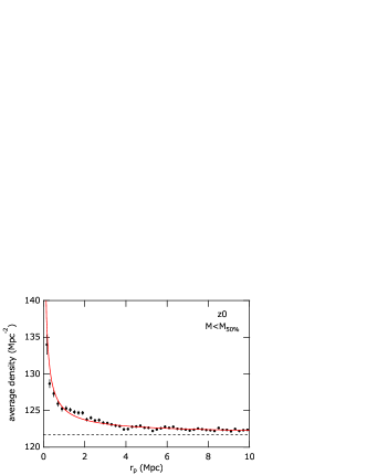
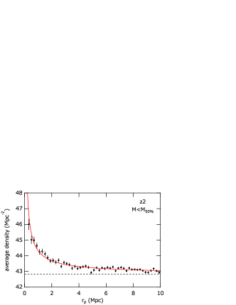
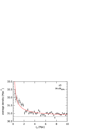
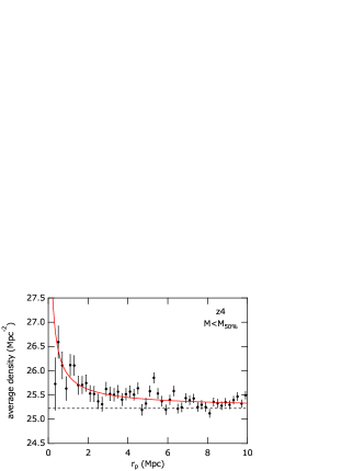
Figure 8: Radial distribution of galaxy surface density around AGNs for each redshift group. $i$-band detected galaxy samples with absolute magnitude brighter than $M_{50\%}$ are used, where $M_{50\%}$ represents the magnitude where detection efficiency is 50%

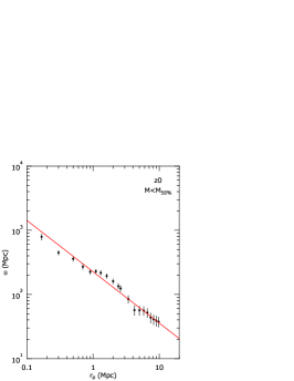
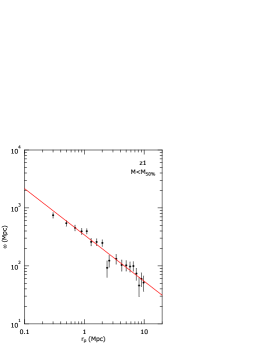
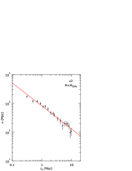
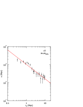
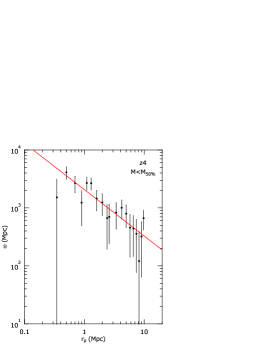
Figure 9: Projected cross-correlation functions derived from data shown in Figure 8. Solid lines represent the power law model fitted to the data.

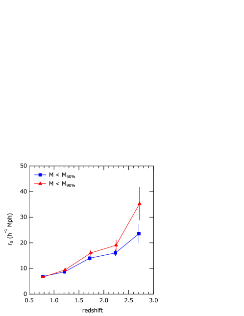
Figure 10: Cross-correlation length as a function of redshift. Squares and triangles represent the cross-correlation length derived using galaxies brighter than $M_{50\%}$ and $M_{90\%}$ respectively, where $M_{50\%}$ ($M_{90\%}$) represents the magnitude where detection efficiency is 50% (90%).

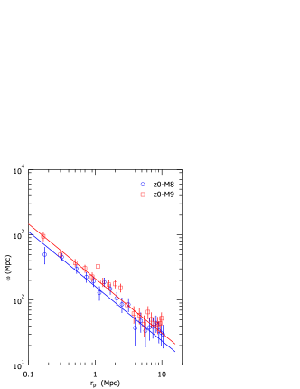
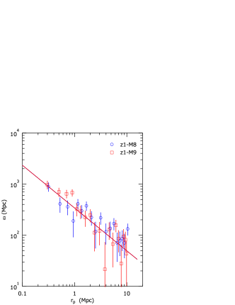
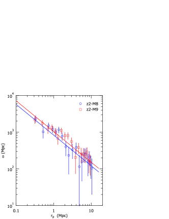
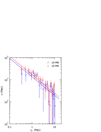
Figure 11: Comparisons of projected cross-correlation functions derived for mass groups of M8 (circles) and M9 (squares). Each panel represents the result for redshift z0, z1, z2, and z3. Redshift-matched AGN samples and galaxy samples brighter than $M_{90\%}$ are used. Solid lines represent the power law model fitted to the data points.

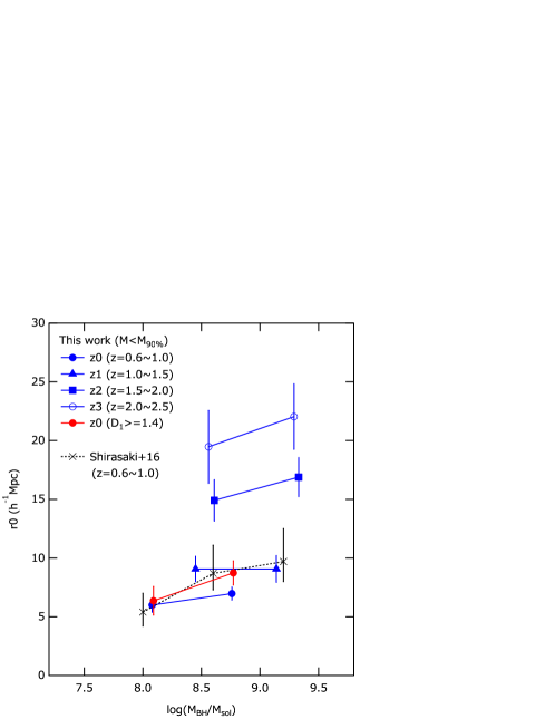
Figure 12: Cross-correlation lengths plotted as a function of average BH mass obtained for data shown in Figure 11 (blue solid markers). Note that the galaxy sample for these datasets are dominated by blue galaxies. The result obtained by Shirasaki+16, for which galaxy samples are dominated by red galaxies contrary to the current dataset, is shown with crosses. The result obtained using the data selected by color to construct a dataset comparable with the result of Shirasaki+16 is shown with open circles.

Fitting result of cross-correlation function. BH mass Redshift $n_{\rm AGN}$${}^{\rm a}$ $\langle\log{M_{\rm BH}/M_{\solar}}\rangle$${}^{\rm b}$ $\langle z\rangle$${}^{\rm c}$ $r_{0}$${}^{\rm d}$ $\langle n_{\rm bg}\rangle$${}^{\rm e}$ $\langle\rho_{0}\rangle$${}^{\rm f}$ $\log{(M_{\rm BH}/M_{\solar})}$ ${h^{-1}{\rm Mpc}}$ Mpc${}^{-2}$ $10^{-3}$Mpc${}^{-3}$ $M<M_{90\%}$ galaxy samples 7.0–11.0 (M8+M9) 0.6–1.0 (z0) 1194 8.45 0.78 6.66$\pm$0.36 76.29$\pm$0.03 11.2 7.0–11.0 (M8+M9) 1.0–1.5 (z1) 1216 8.80 1.22 9.46$\pm$0.69 42.53$\pm$0.02 2.85 7.0–11.0 (M8+M9) 1.5–2.0 (z2) 1235 8.94 1.74 16.05$\pm$1.09 28.73$\pm$0.02 0.886 7.0–11.0 (M8+M9) 2.0–2.5 (z3) 1511 8.96 2.25 19.07$\pm$2.06 20.67$\pm$0.01 0.299 7.0–11.0 2.5–3.0 (z4) 396 8.90 2.72 35.24$\pm$6.41 16.89$\pm$0.02 0.0968 $M<M_{50\%}$ galaxy samples 7.0–11.0 (M8+M9) 0.6–1.0 (z0) 1194 8.45 0.78 6.89$\pm$0.36 121.73$\pm$0.04 15.5 7.0–11.0 (M8+M9) 1.0–1.5 (z1) 1216 8.80 1.22 8.67$\pm$0.58 64.67$\pm$0.03 4.92 7.0–11.0 (M8+M9) 1.5–2.0 (z2) 1235 8.94 1.74 14.02$\pm$0.77 42.82$\pm$0.02 1.85 7.0–11.0 (M8+M9) 2.0–2.5 (z3) 1511 8.96 2.25 16.08$\pm$1.21 30.80$\pm$0.02 0.777 7.0–11.0 2.5–3.0 (z4) 396 8.90 2.72 23.58$\pm$3.62 25.22$\pm$0.03 0.332 Redshift-matched AGN samples & $M<M_{90\%}$ galaxy samples 7.0– 8.4 (M8) 0.6–1.0 (z0) 482 8.08 0.77 6.00$\pm$0.61 75.42$\pm$0.04 11.4 8.4–11.0 (M9) 0.6–1.0 (z0) 482 8.76 0.77 6.98$\pm$0.55 76.44$\pm$0.04 11.4 7.0– 8.8 (M8) 1.0–1.5 (z1) 506 8.45 1.22 9.07$\pm$1.08 42.03$\pm$0.03 2.85 8.8–11.0 (M9) 1.0–1.5 (z1) 506 9.14 1.22 9.07$\pm$1.14 43.05$\pm$0.03 2.86 7.0– 9.0 (M8) 1.5–2.0 (z2) 534 8.61 1.74 14.91$\pm$1.75 28.67$\pm$0.03 0.890 9.0–11.0 (M9) 1.5–2.0 (z2) 534 9.33 1.74 16.89$\pm$1.65 28.95$\pm$0.03 0.887 7.0– 8.9 (M8) 2.0–2.5 (z3) 640 8.56 2.25 19.47$\pm$3.10 20.75$\pm$0.02 0.299 8.9–11.0 (M9) 2.0–2.5 (z3) 640 9.29 2.25 22.04$\pm$2.78 20.61$\pm$0.02 0.300 ${}^{a}$number of AGN datasets, ${}^{b}$average of logarithm of BH mass, ${}^{c}$average redshift, ${}^{d}$cross-correlation length and its error, ${}^{e}$average of projected number density of background galaxies, ${}^{f}$average of the averaged number density of galaxies at the AGN redshift,