SLAM with Objects using a Nonparametric Pose Graph
Abstract
Mapping and self-localization in unknown environments are fundamental capabilities in many robotic applications. These tasks typically involve the identification of objects as unique features or landmarks, which requires the objects both to be detected and then assigned a unique identifier that can be maintained when viewed from different perspectives and in different images. The data association and simultaneous localization and mapping (SLAM) problems are, individually, well-studied in the literature. But these two problems are inherently tightly coupled, and that has not been well-addressed. Without accurate SLAM, possible data associations are combinatorial and become intractable easily. Without accurate data association, the error of SLAM algorithms diverge easily. This paper proposes a novel nonparametric pose graph that models data association and SLAM in a single framework. An algorithm is further introduced to alternate between inferring data association and performing SLAM. Experimental results show that our approach has the new capability of associating object detections and localizing objects at the same time, leading to significantly better performance on both the data association and SLAM problems than achieved by considering only one and ignoring imperfections in the other. 111software is available at https://github.com/BeipengMu/objectSLAM.git 222video is available at https://youtu.be/YANUWdVLJD4
I Introduction
In many robotics applications, such as disaster relief, planetary exploration, and surveillance, robots are required to autonomously explore unknown spaces without an accurate prior map or a global position reference (e.g. GPS). A fundamental challenge faced by the robot is to effectively localize itself using only the information extracted from the environment. For example, the capability of recognizing instances of objects and associating them with unique identifiers will enable the robot to build maps of the environment and localize itself within. The problem of constructing a global map and localizing the robot within is referred as simultaneously localization and mapping (SLAM).
SLAM with various representations of the world and different sensors has been thoroughly studied in the literature. Occupancy grid map with LiDAR or laser range finders is among the early successes that dates back to the 1980s [1, 2, 3, 4]. In occupancy based approaches, the world is represented by 2D/3D grids composed of free spaces and occupied spaces. New scans from the LiDAR or laser range finders are compared and matched with previous scans to incrementally build such maps. This simplified representation of the world facilitates efficient computation, and thus real-time performance can be achieved on relatively large scenes with a single CPU. However, The successful matching of two scans relies on geometric features such as corners. In places that lack such features, like long hallways, SLAM using occupancy grid maps tends to fail. In recent years, SLAM with 3D dense mapping and RGB-D cameras has become more and more popular [5, 6, 7]. This line of work is able to utilize both the geometric information from depth cameras and the color information from RGB cameras to reconstruct environments in dense 3D maps. Incoming depth and color images are converted into volumes or deformation surfaces [5], then matched with previously constructed volumes or surfaces to incrementally build the map. 3D dense maps provide photographic details of the environment with millions of volumes or surfaces. However, they rely heavily on parallel computation enabled by GPUs, and do not scale very well.
A factor graph is a different representation of the SLAM problem [8, 9, 10, 11]. Instead of using small units, such as grids, volumes, or surfaces, to represent the space, a factor graph encodes the poses of the robot and the observed landmarks along the trajectory. In a factor graph, each factor represents a constraint on the relative poses either between two consecutive robot poses or between a robot pose and a landmark. The robot poses and landmark positions are modeled as random variables, and they are optimized by maximizing the joint likelihood. Mechanisms can be designed such that new factors are only added when there are significant pose updates or new object measurements to facilitate concise representation. As a result, Factor graph SLAM scales much better than SLAM with occupancy grid maps or 3D dense maps. However, the convergence of factor graph SLAM algorithms relies heavily on correct data association of the landmarks. Even a single false association can cause the algorithm to diverge [12, 13].
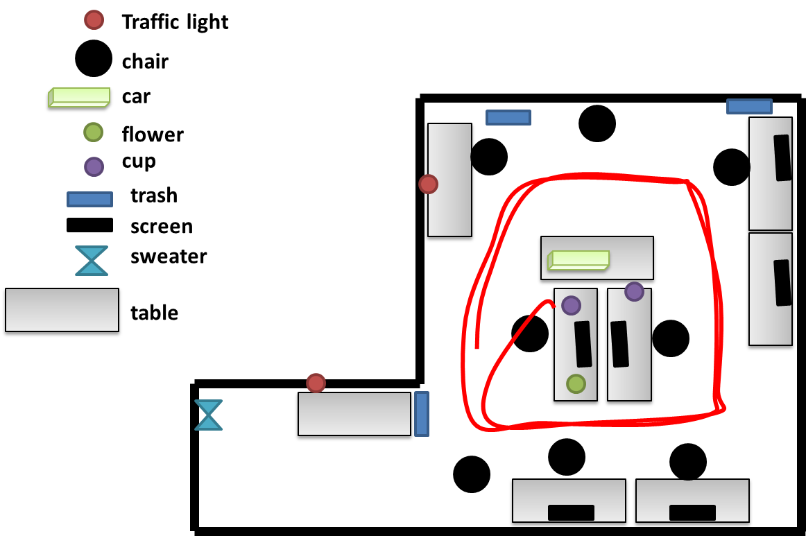
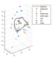
The focus on of this work is on SLAM in unknown environment by recognizing objects and utilizing their positions (object SLAM). A factor graph is the natural representation, as objects can be easily represented as landmarks. A map represented by objects is desirable, as objects are very rich in semantic meanings. By using objects, robots can interact with other agents and perform tasks at semantic level, such as searching for people in a forest, grasping objects, and detecting moving cars on streets. Object SLAM requires the robot to be able to detect objects, generate measurements, and associate these measurements to unique identifiers. In this work, object detection refers to the problem of identifying the occurrence of objects of some predefined object classes within an image. An object measurement is a 3D location of the detected object with respect to the robot pose. Data association refers to the problem of associating object measurements to unique identifiers across images. The problem of object detection has been an important topic in the computer vision community. Deep learning approaches have achieved significant success on object detections within individual images [14, 15, 16, 17, 18]. These approaches also have the ability to generalize: once a detector is trained to recognize a object class, such as chairs, the detector can detect different instances of the same class even in different shape, color, and background settings. Some recent work on Region-based Convolutional Neural Networks [15, 19] gained significant success on training deep learning models to detect multiple objects instances within a single image. However, object detections only suggest the existence of objects of certain predefined object classes in an image, but provide no data association between images. given that an object of a certain class is detected in two images, the object detector provides no information on whether or not the detected objects in the two images are the same object. This is problematic for SLAM especially when there are multiple objects of the same object class in an environment. How reliably SLAM can be achieved using only these ambiguous object detections remains an open question. As illustrated in Figure 1, there are multiple instances of the same object class, such as chairs. The robot would need to establish the data association of object detections across images from different views. Note that data association and SLAM are inherently coupled problems: good data association guarantees the convergence of SLAM algorithms, and good SLAM solution gives good initialization of data association.
This paper proposes a novel world representation, the nonparametric pose graph, to jointly perform data association and SLAM. In the proposed model, factor graphs are used to localize robots and objects, while a Dirichlet process (DP) – a nonparametric model prior – is used to associate detections to unique object identifiers in the scene. The inference of the data associations and the optimization of the the robot and object poses are performed alternatively in this algorithm. This coupled framework achieves better performance for both data association and SLAM.
The contributions of this work are:
-
•
Creating a nonparametric pose graph model that couples data association and SLAM.
-
•
Proposing an algorithm that jointly infers data associations and optimizes robot poses/object locations over nonparametric pose graphs.
-
•
Developing an approach to generate object measurements from RGB and depth images in 3D space via deep learning object detection.
-
•
Demonstrating the performance of the proposed approach via both simulated and real-world data.
II Related Work
Data association of objects and SLAM are typically solved as decoupled problems in the literature. Pillai and Leonard [20] showed that when the SLAM solution is known, and thus there is no uncertainty in robot poses, robot poses provide good prior information about object locations and can achieve better recalls than frame by frame detections. Song et al. [21] used a SLAM solver to build a 3D map of a room, and then fixed the map and manually labeled objects in the room. On the other hand, object detection can improve localization as well. Atanasov et al. [22] pre-mapped doors and chairs as landmarks. During the navigation stage, these pre-mapped objects are detected online and their location information is used to localize the robot.
However, in the scenario considered here, neither data association of objects nor robot poses are perfectly known. The algorithm must associate objects detections and perform SLAM simultaneously. Algorithms that solve object detection and SLAM jointly can be categorized into front-end approaches and back-end approaches.
II-A Front-end Data Association
In front-end approaches, objects detected in new images are compared with previous images. If matches between new and old images are found, then corresponding objects are associated to the same unique identifier. These matches are typically reliable as the disparity between two consecutive images are usually small. When the robot come back to a previously visited place after traversing a long distance, costly global optimization must be performed to achieve global loop closures. These data associations by front-end procedures are taken as reliable and true, and then passed to a SLAM solver [23, 24]. SLAM++ [23] is one such front-end approach. Full 3D scans of chairs and tables are created and used as templates. When new point clouds are observed during testing, they are matched to pre-built templates. Successfully matched detections are often of high credibility. A SLAM solver is then run on these reliable detections to optimize object locations and camera poses. In semantic SLAM [24], Civera et al. created a library of six objects, used SURF features to detect these objects, and then ran an EKF to simultaneously localize robot and map objects.
In this work, instead of creating exact templates for objects, deep learning is used to detect objects in the environment. Deep learning generalizes much better than template-based approaches. It can leverage open source software (millions of images already exist online to create models), scales easily to hundreds of object classes instead of a handful of pre-tuned templates, and does not require the objects in the scene to be exactly the same as the templates. However, the detections have significant ratio of false positives and partial occlusions, thus are very challenging for front-end algorithms to produce reliable data associations.
II-B Back-end Robust SLAM
Robust SLAM is a line of research that explicitly use back-end approaches to deal with outliers in the data [25, 9, 26]. In robust SLAM, most of the object measurements are already correctly associated to unique identifiers. when some measurement is incorrectly associated, it will be inconsistent with other object measurements of the same identifier. Robust SLAM instead maximizes a set of measurements that are consistent with each other in both identifiers and predicted locations. Only the consistent measurements are plugged into a SLAM solver to recover the robot poses and landmark locations.
By nature robust SLAM relies on the assumption that inlier measurements with unique identifier associations are the majority compared to outlier measurements. Under this assumption, eliminating outliers can still give good SLAM results. However, in object SLAM, it is often the case that there are multiple instances of the same object class. If all object measurements with same class are associated to the same identifier, different object instances will always give inconsistent measurements. In other words, in object SLAM, outliers are pervasive. If only one set of consistent measurements for each object class is kept, the algorithm will eliminate the majority of the data and fail to identify any repetitive instances of the same class.
The algorithm presented in this paper is a back-end approach where there are multiple instances of the same object class. The data association of object measurements to unique identifiers are considered unknown and must be established while doing SLAM. We exploit the coupling between data association and SLAM, jointly optimize both, and achieve better performance on both.
III Object Measurements via Deep Learning
This section sets up the approach to generate object measurements via deep learning. The limitations of such an approach are discussed at the end of the section, which highlights the necessity of back-end data association and SLAM algorithms.
III-A Deep Learning Based Object Detection
Object detection refers to the problem of identifying the existence of objects of certain classes and find bounding boxes for them in single images. Object detection in the past decade was mainly based on the use of SIFT and HOG features. Although researchers have developed algorithms that demonstrated good performance for single class object detection (e.g. pedestrians), the multi-class object detection problem remains difficult. In particular, prior to 2012, the state-of-the-art method (deformable part models) achieved 33.4% accuracy on the PASCAL VOC 2010 dataset [15], which contains 20 object classes.
Region-based convolutional neural network (R-CNN) [15] was among the first works on object detection using a CNN. This algorithm uses the selective search [27] algorithm to generate bounding box proposals, and then crops an image patch using each proposal. The image patches are subsequently scaled and run through a CNN model for object detection. This approach achieved 53.7% accuracy on the PASCAL VOC dataset. R-CNN is extremely slow (13 seconds per image) because all patches need to run through the CNN individually.
In Faster R-CNN [19], Ren et. al. ran the full image through the CNN only once, and they only use features in top layer in each bounding box patch for object detection. They further proposed a region proposal network (RPN) that learns how to generate bounding box proposals by looking at the top layer features. This new algorithm achieves 76% accuracy and an average speed of 100 milliseconds per image.
Faster R-CNN [19] uses the VOC dataset for training. Most of the object classes in the VOC dataset [14] are rare in urban or indoor settings, such as cows, horses, sheeps, airplanes, and boats. Our work trained a faster R-CNN model on the ImageNet 2014 dataset [17], which contain categories that are more relevant to indoor/urban settings, including cars, motorcycles, bicycles, traffic lights, televisions, chairs, flowerpots, cups, and keyboards. Note that this framework can be easily modified to parse out any other subset of classes from the ImageNet dataset that are relevant to the specific applications.
III-B Object Measurements
An object measurement refers to a labeled 3D location with respect to the robot pose. To generate such measurements, location information relative to the robot is required in addition to object detection. In this paper, this is done by inquiring the corresponding pixels in the depth images: (1) Crop bounding boxes in the depth image in correspondence with the RGB bounding box. (2) Filter out background pixels that are too far away. (3) Generate point cloud from RGB and depth pairs. (4) Compute the centroid of the point cloud as center of the object.
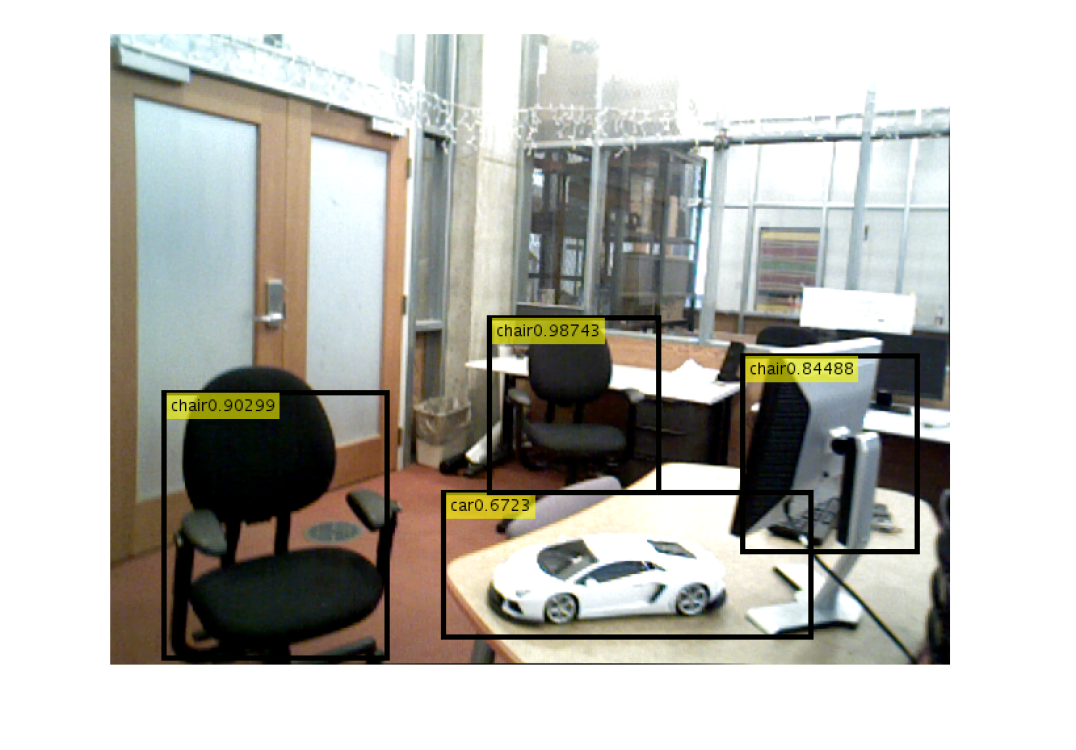
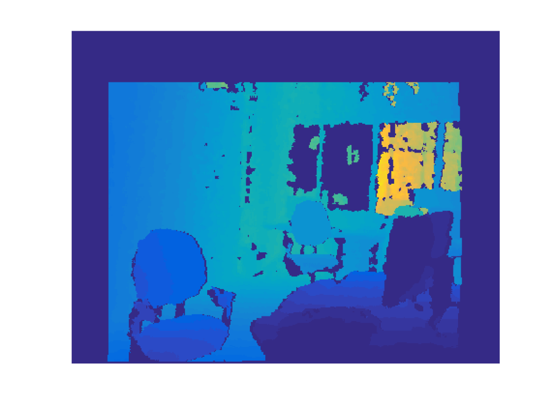
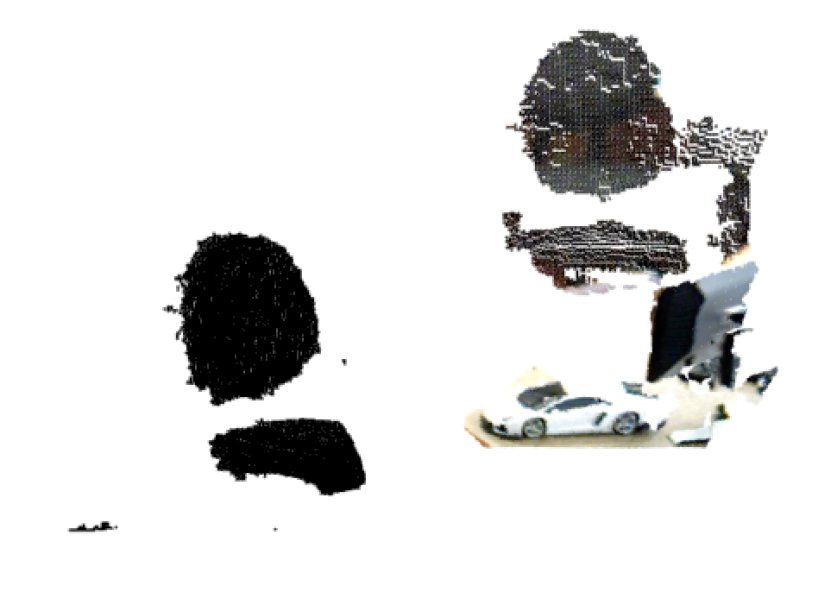
Figure 2(a) shows the detected object with faster R-CNN from a single image of an office environment. Figure 2(b) shows the corresponding depth image, and Fig. 2(c) shows the four point clouds for the four detected objects in 3D space.
It is clear from Fig. 2(a) that object SLAM with deep learning object detection has two major challenges. First, there are multiple instances of the object class, such as “chair” in Fig. 2(a). Without correct data association, it is hard to distinguish different object instances. Standard pose-graph SLAM algorithms can only optimize poses with exact data association, such as g2o[28], isam[10], gtsam[29]. The second challenge is high false positive rates. As the chair detected in Fig. 2(a), deep learning algorithms report objects now and then when there are actually none. Blindly using these unfiltered detections in standard SLAM algorithms will lead to “non-exist” nodes and cause loop closure failures.
Notice that the centroid is used as the center of objects in this case. When objects are looked at from different views, and be partially occluded, centroids would not be a consistent measure of the object locations. In our experience, the error could be 10-20cm. However, we will show that in office settings, our algorithm still converges even under significant occlusion and view point noise.
IV Pose Graph Background
This section sets up the background on graphical models used in SLAM problems. The next section will extend the current pose graph to a novel nonparametric pose graph and introduce an algorithm to perform inference on it.
IV-A Factor Graphs
A graphical model is a probabilistic model that expresses the conditional dependence structure between random variables. Graphical models use a graph-based representation to encode a complete distribution over a high-dimensional space [30]. Commonly used graphical models include Bayesian networks, Markov Random Fields, and factor graphs. Fig. 3 gives an example of such a factor graph. Circles represent random variables and squares represent factors. A factor graph is a graphical model widely used in SLAM problems. Denote as the random variables. Denote as a factor among random variable in set . The the joint probability can be expressed as a product of factors:
| (1) |
where is the set of all factors. Each factor maps the values of random variables to a strictly positive real number representing the likelihood of the variables. It also represents probabilistic dependences among the variables in the factor.
Factor graph is an efficient representation in that it captures sparsity among variables: two variables are independent of each other given all other variables if and only if they do not belong to the same factor. The log likelihood, , can be written in a sum of factors: , where is the set of all factors. Each factor maps the values of random variables to a strictly positive real number representing the log likelihood of the variables. With graphical models, there exist fast algorithms to compute statistical properties such as marginalization, expectation, maximum likelihood [30].
IV-B Factor Graph for SLAM
Factor graphs have gained a lot of success and popularity for SLAM problems [10, 29] due to their efficiency. Fist assume that there exist static landmarks that the robot can identify to localize itself.
Assumption 1
There exists a library of static landmarks to localize the robot in the environment. The number and locations of these landmarks is not known a priori.
With the landmark assumption, when moving in the environment, the robot can obtain measurements of these landmarks. Given a dataset, the robot trajectory is represented as a discrete sequence of poses. Denote as the total number of time steps, and denote as the robot’s trajectory from the start to the end. Each robot pose consists of a position and an orientation. Denote as the space of 2D poses and as the space of 3D poses. Then for 2D cases and in 3D cases. In GPS-denied environments these poses are not directly observable. However, the robot can always measure the incremental change between two sequential poses via an IMU or wheel encoder, which is referred to as odometry. Denote as the odometry measurement between pose and pose . Under the standard assumption that is corrupted by additive Gaussian noise, the odometry measurement at time can be represented as:
| (2) |
where represents an operator that takes two pose and return the relative pose between them in or , and is the odometry noise covariance matrix. The likelihood of given the two poses is then:
| (3) |
During navigation, the robot also observes landmarks from the environment. Assuming that there exist landmarks in the environment, which might be unknown ahead of time. The positions of the landmarks are denoted as . In the 2D case , and in the 3D case . At time , the robot obtains landmark measurements, denoted as . Each measurement is associated to a unique landmark identifiers, the associations are denoted as , where . For example, at time 0, the robot obtained two measurements, . And these 2 measurements are from landmark 5 and 7, then .
Using the standard model that object measurements are corrupted by additive Gaussian noise:
| (4) |
where is the measurement noise matrix. The likelihood of given the robot pose, the landmark association and landmark pose is then:
| (5) |
Combining Equation 2 and and Equation 4, the joint log likelihood of odometry and landmark measurements is:
| (6) |
where and are odometry and landmark factors respectively. Using the probability distribution formula for Gaussian noise, it can be shown that each factor follows a quadratic form:
| (7) |
The pose graph SLAM problem optimizes robot poses and object locations such that the log likelihood is maximized:
| (8) |
Note that the log likelihood is nonlinear in and as is a nonlinear operation in Equation 2 and Equation 4.
A factor graph representation for SLAM is also referred to as a pose graph. Figure 4 illustrates such a pose graph. Variables represent either a robot pose or a landmark. And factors are either odometry or landmark measurements.
V Nonparametric Pose Graph
This section sets up the joint data association and SLAM problem by extending the current pose graph to a novel nonparametric pose graph that tightly couples object association with robot poses. A new algorithm is also introduced to jointly infer the data association and perform SLAM with this new model.
V-A Factor Graph with Multi-class Objects
Before we move into nonparametric factor graph for imperfect data association, first notice in object SLAM, except for measuring the 3D location of objects, we also observe an object class. The observed object class is not always reliable, thus we first establish the probabilistic model for object classes. Assume there are object classes in total. For object , denote as an observation of the object class. The likelihood of is modeled with a Categorical distribution:
| (9) |
Denote , . And if the true object class is , we have for .
Notice , but we especially design to represent the probability of false positives. This design would help the algorithm to filter non-exist object detections in real-world experiments.
In order to have closed form updates, we apply Dirichlet prior to for object :
| (10) |
when there is an observation of class , , the posterior distribution of is:
| (11) |
where represents a unit vector with th element to be 1.
Notice represents the initial likelihood of object to be a false positive. Since observations cannot be 0, when there are more and more observations of object being obtained, the posterior will monotonically decrease. This is consistent with the intuition that if repeated observations are obtained from some object, then it has lower chance to be a false positive.
Combine the multi-class probabilistic setting with the original SLAM problem: each object measurement would be a pair , where continuous variable represents the 3D location measurement, and discrete variable represents the observed object class. Recall that represents that the -th measurement at time is from object . Then is a sample from the posterior distribution .
| (12) |
The joint log likelihood becomes:
| (13) |
The new optimization problem is then
| (14) |
Compared to (8), the observed data in problem (14) further includes object class observations , and the variables to be estimated further include the class of objects . From (V-A), given data association , the joint likelihood can be factorized into the sum of likelihood of and , and the likelihood of . Therefore, the class classes is independent of the robot poses and object positions . Optimizing (14) is equivalent to solving problem (8) and computing the object class posterior independently.
V-B Nonparametric Pose Graph
Now we move to the case that the data association is unknown and must be established. Deep learning-based algorithms label each object to be of some class, but do not distinguish between different objects of the same class. When there are multiple instances of the same object class, such as multiple chairs in a room, possibilities for data association become combinatorial and thus challenging. Instead of relying on a reliable front-end procedure to associate objects, we use a back-end framework to jointly infer the data association and object locations. Note that Because of the ambiguous data association, the total number of objects is unknown ahead of time, and needs to be established as well. Nonparametric models are a set of tools that adapt the model complexity to data. It has the embedded mechanism that the model parameters could grow when there are new data being observed. In particular, Dirichlet Process (DP) is such a nonparametric stochastic process that models discrete distributions but with flexible parameter size. It can be taken as the generalization of a Dirichlet distribution with infinite dimension. Same as Dirichlet distribution is the conjugate prior for a categorical distribution, DP can be viewed as the conjugate prior for infinite, nonparametric discrete distributions [31]. In this work, we use a Dirichlet Process (DP) as the prior for data associations . In particular, assume at any point, there are objects being detected in total, the probability of belongs to object :
| (17) |
where is the number of measurements of object , and is the concentration parameter of DP prior that determines how likely it is to create a new object. The intuition behind this model is that the probability is from some existing object is proportional to the number of measurements of object , and the probability is from a new object is proportional to .
The joint log likelihood of odometry , object measurement and object classes given data association is
The joint log likelihood (V-B) has the same form as (V-A). However, in (V-B), the likelihood of object measurements and object classes are correlated through data association .
The new optimization problem is then over The joint log likelihood of odometry , object measurement and object classes given data association :
| (18) |
Compared with Equation 8, the new optimization problem Equation 18 is more challenging in that data associations are unknown. As a result, log probabilities of object measurements no longer have a simple form, and the problem Equation 18 becomes a mixed integer nonlinear problem. Secondly, the number of true objects in the environment is not necessarily known a priori, problem Equation 18 must infer at the same time.
V-C Nonparametric SLAM
From the last section, for , the generative model for our problem is
| (19a) | ||||
| (19b) | ||||
| (19c) | ||||
| (19d) | ||||
| (19e) | ||||
where , , , and are given parameters. Robot poses , landmark locations , object class distributions and object associations are variables to be estimated. The odometry and object measurements are observed data.
Different from a canonical DP mixture model, the observed data , , and are not independent samples given variables , , and , but are correlated through the factor graph. Therefore, the inference involves computing maximum likelihood over factor graphs. When both associations and variables are to be established, standard approaches alternate between assigning data and optimizing variables. In the case of known object number , K-means has a deterministic data association, while expectation-maximization associates data in a probabilistic way [30]. When the number of objects is not known a priori and DP is used as prior, Markov Chain Monte Carlo methods (e.g. Gibbs sampling) or variational inference algorithms are widely used [30]. However, in these algorithms, the likelihood of each label to be any underlying object needs to be computed and tracked all the time. The algorithm will need to go through all of the data multiple times to converge to a steady state distribution. The large scale and strong dependence of data in our problem make such approaches inappropriate.
It is shown in [32] that under the small variance assumptions, Gibbs sampling can be simplified to DPmeans. Instead of sampling the posterior distribution, is assigned to be the maximum likelihood object if the likelihood is within some certain threshold, otherwise it is assigned to a new object. Intuitively, in this case, small variance means that the noise in odometry, object measurement and object class is relative small, so that the posterior distribution of is peaky.
Assumption 2
Variance in odometry, object measurement and object class is small, so that the posterior distribution of data association has small variance and a unique maximal likelihood value.
The DPmeans algorithm alternates between two steps: maximize likelihood on variables , and assign data association to their maximum likelihood objects. Algorithm 1 shows the overall flow of the approach. And the following explains the algorithm step by step.
Initialization (line 3)
In initialization, all are set to be an object by its own. Robot poses and object locations are initialized by their open loop estimation. The Dirichlet distribution prior for object class are set to be some initial value .
Optimizing data association (line 5)
While executing the main loop, the algorithm alternates between optimizing associations , and variables , , and . When optimizing object association, fix , and , and compute the posterior of as the product of its DP prior (17) and likelihood of measurements (see (2) and (12)).
| (20) |
Then is assigned to the maximum likelihood object
| (21) |
Optimizing poses (line 12)
When optimizing poses, object associations are fixed. The posterior parameters for the Dirichlet distribution of object class can be updated with
| (22) |
where is the hyper parameter for the Dirichlet prior on . Notation represents indicators whether quantity equals quantity . Then is the total number of object detections assigned to object , and represents from the detections of object , how many are class . With Dirichlet prior , the maximum likelihood(ML) of each object class is proportional to parameters :
| (23) |
The maximum likelihood value of robot poses and object locations can then be obtained by standard SLAM solvers (see (8)).
Remove false positive (line 20)
Recall that we set to be the probability that object is a false positive. In initialization, is set to be some positive number. When new measurements of object are obtained and accumulated, gets updated such that , becomes bigger compared to . As a result, decrease monotonically. In the last step, we filter out false positives by simply putting a threshold on .
VI Experiment
VI-A Simulated Dataset
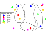
In the simulation, 15 objects are randomly generated in a 2D plane. They are randomly assigned into 5 different object classes: red diamonds, blue circles, green triangles, yellow stars, and magenta squares. The robot trajectory is manually designed and passes through the environment several times. Figure 7(a) shows the ground truth of the generated dataset. At each pose , the robot observes the relative position and class of the objects that are within its field of view. Gaussian noise are added to the odometry measurements as well as object measurements, see (2), and (4). The parameters of the dataset are listed in Table I.
| Distance Traveled | 72.7m |
|---|---|
| field of view | 4m, 120 degree |
| no. of odometry measurements | 766 |
| no. of object measurements | 1098 |
| odometry noise | |
| measurement noise |
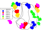
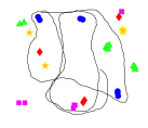
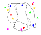
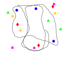
Figure 6(a) shows the object predictions based purely on open-loop odometry. There is significant amount of variance and drift in the distribution of these predicted object locations, which obscures the determination of exactly how many objects there actually are in the environment. The result after the first iteration is shown in figure 6(b); the nonparametric pose graph clusters the measurements and uses it to correct robot poses. The total number of objects is reduced to 33. The result after the second iteration is shown in figure 6(c); the algorithm further reduces the total number of objects to 20. After three iterations(figure 6(d)), the algorithm converges to the true underlying number of objects, which is 15.
The performance of the proposed nonparametric graph (NP-Graph) is compared to three existing methods:
-
1.
Frame by frame detection (FbF): each object in each frame is taken as new, and there are neither SLAM nor data association (see Fig. 6(a)).
-
2.
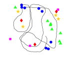
Open-loop Object Detection (OL): use robot odometry to perform data association across images, but do not use data association results to correct robot poses (see Fig. 7(c)).
-
3.
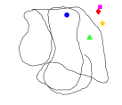
Robust SLAM (R-SLAM): back-end algorithm that finds the maximal set of consistent measurements, but eliminate inconsistent measurements (see Fig. 7(b)).
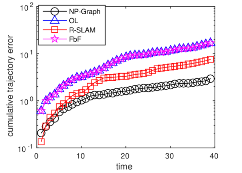
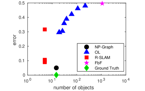
Figure 7 and Table II compare the SLAM performance results of four different algorithms. Figure 8 shows the cumulative position error of the robot trajectory compared to ground truth, while Figure 9 compares the number of objects identified and their localization error with a variety of parameter settings for the R-SLAM and OL approaches. FbF and OL purely rely on odometry and do not correct robot poses, therefore have the biggest error. R-SLAM uses a subset of object measurements to close loops on robot poses, thus the error is smaller. Our NP-graph based approach make use of all the object measurements, thus has the smallest error on both robot poses and object positions. FbF does not do any data association, thus significantly over estimate the number of objects. The OL approach does not optimize robot poses. When the robot comes back to a visited place, the odometry has drifted significantly thus the OL approach could not associate the objects to the same one observed before. As a result, the OL approach also over estimate the total number of objects. R-SLAM only keeps one set of consistent measurements for each object class, therefore it is only able to detect one instance for each object class, and significantly underestimate the total number of objects. NP-Graph, on the other hand, utilize all of the object measurements and jointly infers both robot poses and the data associations, thus can correctly infer the right number of objects.
| mean | cumulative | percent of | number | mean | |
| pose | trajectory | measurements | of | object | |
| error | error | used | objects | error | |
| NP-Graph | 0.07 | 55.1 | 100 | 15 | 0.05 |
| OL | 0.42 | 320.6 | 100 | 39 | 0.39 |
| R-SLAM | 0.20 | 150.5 | 20.2 | 5 | 0.20 |
| FbF | 0.42 | 320.6 | 100 | 1098 | 0.49 |

VI-B Office Environment
To test the performance in real-world scenarios, we collected a dataset of an office environment and used deep learning to detect objects, such as chair, screen, cups etc. The statistics about the office dataset is shown in Table III.
| image resolution | 640480 |
|---|---|
| distance traveled | 28.06m |
| during | 167s |
| no. of odometry | 696 |
| no. of objects | 30 |
| no. of object detections | 1588 |
| odometry noise | |
| measurement noise |
Table IV and Figure 10 compare the performance of FbF, R-SLAM, OL and our approach NP-Graph. While the ground truth for object positions is not available for this dataset, we compare the performance on the number of valid objects, the number of inlier measurements and the variance on object positions. An object is defined as valid when its false positive probability is below a threshold (), otherwise it is marked as a false positive. A measurement is denoted as an inlier when it is associated with a valid object. The object variance is determined from the uncertainty in the predicted location of the object from its associated measurements. From Table IV, the NP-Graph has the highest percentage of inlier measurements, the closest number of objects to truth, and the smallest variance on the object locations.
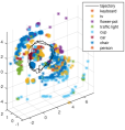
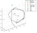
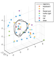
While the ground truth for robot poses is not available, either, we compare the performance qualitatively. Figure 1 shows the floor map of the environment as well as the robot trajectory. Figure 10 compares the results of 4 approaches. FbF and OL estimation are open-loop approaches and over estimate total number of objects. R-SLAM only uses a subset of the object measurements. It can only identify one instance for each object class, and has bad estimates even it closes loops on robot poses. On the other hand, NP-Graph is able to close loops on robot poses and recover the turnings at corners. While there is no ground truth in the office dataset for computing object localization errors, it is worth noting that there is a sweater hanging on the shelf in the far bottom left corner, our algorithm is able to recover its distance while other approaches failed to.
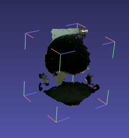
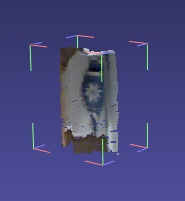
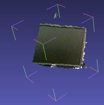
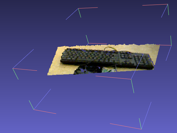
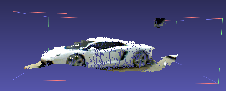
Figure 11 shows a few examples of the detected and well associated objects, which includes chair, screen, keyboard, toy car and the sweater hanging in the back corner. These figures are extracted from point cloud of a single bounding box that is associated to the corresponding object. Note that these point clouds are only for illustration purposes, but not maintained in the algorithm. The algorithm only uses the centroid of these point clouds as object measurements.
| percentage of | number of | number of | variance | |
| measurement | inlier | false positive | on | |
| inliers | objects | objects | objects | |
| NP-Graph | 88.0 | 31 | 88 | 0.058 |
| OL | 82.2 | 36 | 175 | 0.121 |
| R-SLAM | 22.5 | 7 | 0 | 0.225 |
| FbF | 0 | 0 | 1588 | - |
VII conclusion
Object SLAM is challenging as data association is ambiguous and location measurements unknown. Data association and SLAM are inherently coupled problems. This work proposed a novel nonparametric pose graph that tightly couples these two problems, and developed an algorithm to alternative between inferring data association and performing SLAM. Both simulated and real-world datasets show that our new approach has the capability of doing data association and SLAM simultaneously, and achieves better performance on both associating object detections to unique identifiers and localizing objects.
ACKNOWLEDGMENTS
This research is supported in part by ARO MURI grant W911NF-11-1-0391, ONR grant N00014-11-1-0688 and NSF Award IIS-1318392.
References
- [1] A. Elfes. Occupancy grids: A stochastic spatial representation for active robot perception. In Sixth Conference on Uncertainty in AI, pages 7–24, 1990.
- [2] A. Elfes. Using occupancy grids for mobile robot perception and navigation. Computer, 22(6):46–57, june 1989.
- [3] S. Thrun. Learning occupancy grids with forward sensor models. Autonompous Robots, 15:111–127, 2003.
- [4] S. Thrun, W. Burgard, and D. Fox. Probabilistic Robotics. The MIT press, Cambridge, Massachusetts, USA, 2005.
- [5] T. Whelan, S. Leutenegger, R. S. Moreno, B. Glocker, and A. Davison. Elasticfusion: Dense slam without a pose graph. In Proceedings of Robotics: Science and Systems, Rome, Italy, July 2015.
- [6] M. Keller, D. Lefloch, M. Lambers, S. Izadi, T. Weyrich, and A. Kolb. Real-time 3d reconstruction in dynamic scenes using point-based fusion. In 3D Vision - 3DV 2013, 2013 International Conference on, pages 1–8, June 2013.
- [7] R. A. Newcombe, S. Izadi, O. Hilliges, D. Molyneaux, D. Kim, A. J. Davison, P. Kohli, J. Shotton, S. Hodges, and A. Fitzgibbon. Kinectfusion: Real-time dense surface mapping and tracking. In IEEE ISMAR. IEEE, October 2011.
- [8] I. Mahon, S.B. Williams, O. Pizarro, and M. Johnson-Roberson. Efficient view-based SLAM using visual loop closures. Robotics, IEEE Transactions on, 24(5):1002–1014, Oct. 2008.
- [9] M.C. Graham, J.P. How, and D.E. Gustafson. Robust incremental slam with consistency-checking. In Intelligent Robots and Systems (IROS), 2015 IEEE/RSJ International Conference on, pages 117–124, Sept 2015.
- [10] D.M. Rosen, M. Kaess, and J.J. Leonard. An incremental trust-region method for robust online sparse least-squares estimation. In Robotics and Automation (ICRA), 2012 IEEE International Conference on, pages 1262–1269, May 2012.
- [11] M. Kaess, H. Johannsson, R. Roberts, V. Ila, J. J. Leonard, and F. Dellaert. iSAM2: Incremental smoothing and mapping using the Bayes tree. The International Journal of Robotics Research, 31(2):216–235, 2012.
- [12] Michael Montemerlo and Sebastian Thrun. Simultaneous localization and mapping with unknown data association using fastslam. In Robotics and Automation, 2003. Proceedings. ICRA’03. IEEE International Conference on, volume 2, pages 1985–1991. IEEE, 2003.
- [13] M.C. Graham, J.P. How, and D.E. Gustafson. Robust incremental slam with consistency-checking. In Intelligent Robots and Systems (IROS), 2015 IEEE/RSJ International Conference on, pages 117–124, Sept 2015.
- [14] M. Everingham, L. Van Gool, C. K. I. Williams, J. Winn, and A. Zisserman. The pascal visual object classes (voc) challenge. International Journal of Computer Vision, 88(2):303–338, June 2010.
- [15] R. Girshick, J. Donahue, T. Darrell, and J. Malik. Rich feature hierarchies for accurate object detection and semantic segmentation. In Computer Vision and Pattern Recognition (CVPR), 2014 IEEE Conference on, pages 580–587, 2014.
- [16] Christian Szegedy, Alexander Toshev, and Dumitru Erhan. Deep neural networks for object detection. In C.j.c. Burges, L. Bottou, M. Welling, Z. Ghahramani, and K.q. Weinberger, editors, Advances in Neural Information Processing Systems 26, pages 2553–2561. 2013.
- [17] O. Russakovsky, J. Deng, H. Su, J. Krause, S. Satheesh, S. Ma, Z. Huang, A. Karpathy, A. Khosla, M. Bernstein, A. C. Berg, and F. Li. ImageNet Large Scale Visual Recognition Challenge. International Journal of Computer Vision (IJCV), 115(3):211–252, 2015.
- [18] Dumitru Erhan, Christian Szegedy, Alexander Toshev, and Dragomir Anguelov. Scalable object detection using deep neural networks. In Proceedings of the 2014 IEEE Conference on Computer Vision and Pattern Recognition, CVPR ’14, pages 2155–2162, Washington, DC, USA, 2014. IEEE Computer Society.
- [19] S. Ren, K. He, R. Girshick, and J. Sun. Faster R-CNN: Towards real-time object detection with region proposal networks. In Advances in Neural Information Processing Systems (NIPS), 2015.
- [20] S Pillai and J. Leonard. Monocular slam supported object recognition. In Proceedings of Robotics: Science and Systems, Rome, Italy, July 2015.
- [21] S. Song, L. Zhang, and J. Xiao. Robot in a room: Toward perfect object recognition in closed environments. CoRR, abs/1507.02703, 2015.
- [22] N. Atanasov, M. Zhu, K. Daniilidis, and G. Pappas. Semantic localization via the matrix permanent. In Proceedings of Robotics: Science and Systems, Berkeley, USA, July 2014.
- [23] R.F. Salas-Moreno, R.A. Newcombe, H. Strasdat, P.H.J. Kelly, and A.J. Davison. Slam++: Simultaneous localisation and mapping at the level of objects. In Computer Vision and Pattern Recognition (CVPR), 2013 IEEE Conference on, pages 1352–1359, June 2013.
- [24] J. Civera, D. Galvez-Lopez, L. Riazuelo, J.D. Tardos, and J. M. Montiel. Towards semantic slam using a monocular camera. In Intelligent Robots and Systems (IROS), 2011 IEEE/RSJ International Conference on, pages 1277–1284, Sept 2011.
- [25] N. Sunderhauf and P. Protzel. Towards a robust back-end for pose graph slam. In Robotics and Automation (ICRA), 2012 IEEE International Conference on, pages 1254–1261, May 2012.
- [26] Y. Latif, C. Cadena, and J. Neira. Robust loop closing over time for pose graph slam. The International Journal of Robotics Research, 2013.
- [27] Jasper RR Uijlings, Koen EA van de Sande, Theo Gevers, and Arnold WM Smeulders. Selective search for object recognition. International journal of computer vision, 104(2):154–171, 2013.
- [28] g2o: A general framework for graph optimization. https://openslam.org/g2o.html.
- [29] F. Dellaert. Factor graphs and gtsam: A hands-on introduction. Technical Report GT-RIM-CP&R-2012-002, GT RIM, Sept 2012.
- [30] C. M. Bishop. Pattern Recognition and Machine Learning (Information Science and Statistics). Springer, 1st edition, 2007.
- [31] T. Ferguson. A Bayesian Analysis of Some Nonparametric Problems. The Annals of Statistics, 1(2):209–230, 1973.
- [32] B. Kulis and M. I. Jordan. Revisiting k-means: New algorithms via bayesian nonparametrics. In Proceedings of the 29th International Conference on Machine Learning (ICML), pages 513–520, 2012.