The Lyman Continuum Escape and ISM properties in Tololo 1247-232 – New Insights from HST and VLA

Abstract

Low- and intermediate mass galaxies are widely discussed as cause of reionization at redshift $z\sim 10-6$. However, observational proof of galaxies that are leaking ionizing radiation (Lyman continuum; LyC) is a currently ongoing challenge and the list of LyC emitting candidates is still short. Tololo 1247-232 is among those very few galaxies with recently reported leakage. We performed intermediate resolution ultraviolet (UV) spectroscopy with the Cosmic Origins Spectrograph (COS) onboard the Hubble Space Telescope and confirm ionizing radiation emerging from Tololo 1247-232. Adopting an improved data reduction procedure, we find that LyC escapes from the central stellar clusters, with an escape fraction of 1.5$\pm$0.5% only, i.e. the lowest value reported for the galaxy so far. We further make use of FUV absorption lines of Si II and Si IV as a probe of the neutral and ionized interstellar medium. We find that most of the ISM gas is ionized, likely facilitating LyC escape from density bounded regions. Neutral gas covering as a function of line-of-sight velocity is derived using the apparent optical depth method. The ISM is found to be sufficiently clumpy, supporting the direct escape of LyC photons. We further report on broadband UV and optical continuum imaging as well as narrowband imaging of Ly$\upalpha$, H$\upalpha$ and H$\upbeta$. Using stellar population synthesis, a Ly$\upalpha$ escape fraction of 8% was derived. We also performed VLA 21cm imaging. The hydrogen hyperfine transition was not detected, but a deep upper limit atomic gas mass of $\lesssim 10^{9}M_{\odot}$ could be derived. The upper limit gas fraction defined as $\nicefrac{{M_{HI}}}{{M_{*}}}$ is only 20%. Evidence is found that the H I gas halo is relatively small compared to other Lyman Alpha emitters.

1 Introduction

Our current understanding of the cosmological evolution after the Big Bang is well described within the $\Lambda$CDM model which implies two ages of major gas phase changes. The recombination, caused due to the rapid cooling of the Universe after $\sim 400$ thousand years at $z\sim 1090$, and the reionization, that gradually ionized the Universe until $z\sim 6$ (Fan et al., 2001, 2006) corresponding to an age of $\sim 1$ Gyr. As cause of reionization several mechanisms are discussed, such as accreting black holes or Pop III stars (Madau et al., 2004; Trenti & Stiavelli, 2009; Volonteri & Gnedin, 2009; Mirabel et al., 2011; Finlator et al., 2016), but low- and intermediate mass galaxies seem to be the top candidate, given that some fraction of their ionizing radiation was able to escape into the intergalactic medium. However, most of the galaxies observed yet did not show any signs of such Lyman continuum (LyC) emission, but upper limits could be derived by various authors: e.g. Leitherer et al. (1995); Deharveng et al. (2001) for galaxies in the local Universe and Siana et al. (2007); Cowie et al. (2009); Rutkowski et al. (2015) for galaxies at $z\sim 1$. Nevertheless, LyC escape of galaxies at $z\sim 3$ was reported by Iwata et al. (2009); Nestor et al. (2011); Mostardi et al. (2015); Micheva et al. (2015), but could be suffering from foreground contamination (Siana et al., 2007; Vanzella et al., 2010). So far, the most convincing cases of LyC leakage in individual galaxies at high redshift were recently published by Vanzella et al. (2016) and de Barros et al. (2016).

Local galaxies that can be observed at high resolution, exhibiting LyC leakage thus may shed light onto the mechanisms that allow LyC photons to escape. However, despite many observational efforts have been made in the past to detect escaping LyC radiation in galaxies at all redshifts (Bergvall et al., 2013), the list of candidates is still short, in particular at low redshifts where LyC observations are possible only through space-based observatories such as FUSE, the Far-Ultraviolet Spectroscopic Explorer (Moos et al., 2000) or the Hubble Space Telescope (HST). To date, only few local galaxies have confirmed LyC detections. First discoveries were made in Haro11 (Leitet et al., 2011), Mrk 54 (Leitherer et al., 2016), Tololo 1247-232 (Leitet et al., 2013; Leitherer et al., 2016) and J0921+4509 (Borthakur et al., 2014). The published LyC escape fractions are 3.3$\pm$0.7% (Haro11), 2.5$\pm$0.72% (Mrk 54), 4.5$\pm$1.2% (Tololo 1247-232) and 21$\pm$5% (J0921+4509). Recent publications by Izotov et al. (2016a, b) further add five other sources to the list, with the highest measured escape fraction found in J0925+1403 (7.8$\pm$1.1%).

Yet, in order to understand if galaxies could have reionized the Universe, we need to find links between readily accessible observables and the escape of ionizing photons. That way, the number of known LyC leakers could be drastically increased, allowing to disentangle the complex physical processes driving LyC escape. Work done by Zastrow et al. (2011, 2013) suggest that so called indirect tracers such as ionization-parameters can provide such a link. That followed, Jaskot & Oey (2013) suggest that a high [O III]$\uplambda$5007/[O II]$\uplambda$3727 ratio as typically observed in Green Pea galaxies could give rise to leakage of ionizing radiation, because optically thin nebulae should underproduce [O II] (Pellegrini et al., 2012). Hence, high [O III]$\uplambda$5007/[O II]$\uplambda$3727 ratios may also indicate a low LyC optical depth. Another indirect approach was described by Heckman et al. (2011), who argue that non-saturated optically thick FUV metal absorption lines of C II or Si II can be used as a proxy for Lyman continuum, since residual line flux along the absorption spectrum may indicate the presence of channels with low column densities within a medium filled with optically thick clouds, i.e. in agreement with the picket-fence model (Heckman et al., 2001). Since typical H I column densities in galaxies are easily high enough to prevent LyC escape, in the picket-fence model, starbursts could create a sufficiently porous ISM allowing the ionizing radiation from the massive stars to escape through low density areas or voids. Another spectral line discussed in various previous studies that may give rise to Lyman continuum emission, is escaping Ly$\upalpha$ radiation. This is particular interesting, because coupling between Ly$\upalpha$ and LyC (Verhamme et al., 2015) would further mean a big step forward towards understanding the importance of Ly$\upalpha$ emitters (LAEs) during the epoch of reionization, given the large and increasing number of LAEs observed in the early Universe, exactly as needed for reionization (Stark, 2010; Curtis-Lake et al., 2012). In that context the works by e.g. Nakajima & Ouchi (2014) and Henry et al. (2015) seem promising, since they find that the high Ly$\upalpha$ escape fractions in their samples are related to a low H I column density rather than outflow velocity or H I covering fraction.

Luckily, various models and simulations show that the ionizing photon escape increases with decreasing dark matter halo mass (Yajima et al., 2011; Ferrara & Loeb, 2013; Paardekooper et al., 2013; Wise et al., 2014), making LAEs even more promising to be good candidates for LyC leakage. Additionally, cosmological hydrodynamic simulations performed by e.g. Yajima et al. (2014) find a relation between the emergent Ly$\upalpha$ radiation and the ionizing photon emissivity of LAEs. This is further supported by Dijkstra et al. (2016) who performed Monte-Carlo radiative transfer simulations through models of dusty, clumpy interstellar media. The authors find that the ionizing escape fraction is strongly affected by the cloud covering factor, which implies that LyC leakage is closely connected to the observed Ly$\upalpha$ spectral line shape, because the escape of ionizing photons requires that sightlines with low column densities exist, i.e. $N_{HI}\lesssim 10^{17}\,cm^{-2}$. These same channels of low column density then also provide escape routes for Ly$\upalpha$ photons (Behrens et al., 2014; Verhamme et al., 2015); leading to Ly$\upalpha$ halos that are comparably small.

In this paper, using our newly obtained HST FUV spectra of Tololo 1247-232 (see basic parameters in Table 1), along with direct observations of the Lyman continuum, we are able to test the previously described method of Heckman et al. (2011) through FUV Si II absorption lines. Our observation of the Ly$\upalpha$ line allows us to discuss coupling between LyC and Ly$\upalpha$ as proposed by Verhamme et al. (2015) and using VLA 21 cm data, we are further able to make constraints on the atomic gas reservoir of Tololo 1247-232. Additionally, we have obtained HST narrowband imaging. A false-color composite of the galaxy encoding the morphology of Ly$\upalpha$, H$\upalpha$ and UV continuum is shown in Figure 1. Given the amount of high quality data now available, we eventually discuss the driving mechanisms and physical quantities behind the LyC of Tololo 1247-232 (hereafter Tol1247). Throughout the paper, we adopt a cosmology with H${}_{0}=70$, $\Omega_{M}=0.3$ and $\Omega_{vac}=0.7$. The measured redshift of Tol1247 is $z=0.0488\pm 0.0002$, which results in a luminosity distance of 216.8 Mpc.

parameter	value	reference
redshift	$z=0.0488\pm 0.0002$	see caption
luminosity dist.	$216.8\,Mpc$	from $z$ (W06)
stellar mass	$M_{*}=5\times 10^{9}\ M_{\odot}$	L13
atomic gas mass	$M_{HI}\lesssim 10^{9}\ M_{\odot}$	this work 3.10
gas fraction	$\nicefrac{{M_{HI}}}{{M_{*}}}\lesssim 0.2$	this work 4.1
star formation rate	SFR${}_{H\upalpha,0,SB}=36.2\,M_{\odot}\,yr^{-1}$	this work 3.8
metallicity	$12+log\big{(}\nicefrac{{O}}{{H}}\big{)}=8.1\ or\ \approx\nicefrac{{1}}{{4}}Z_{\odot}$	T93

Table 1: Basic parameters of Tololo 1247-232. The redshift was measured from optical emission lines by Emily Freeland (Stockholm University) using ALFOSC slit spectra obtained at the Nordic Optical Telescope. Reference codes are W06 for Ned Wright’s cosmology calculator (Wright, 2006), L13 is Leitet et al. (2013) and T13 is Terlevich et al. (1993).

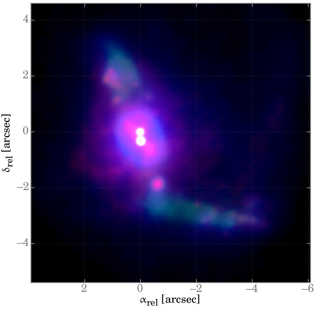
Figure 1: RGB false-color composite showing H$\upalpha$ in $red$, Ly$\upalpha$ in $blue$ and the UV continuum in $green$. Each plane was scaled and smoothed individually to emphasize on morphological differences between the individual components. The coordinates are relative to the center of the COS aperture. North is up, east is left.

2 Observations and Data Reduction

2.1 HST/COS FUV Spectroscopy

FUV spectroscopy was performed using the Cosmic Origins Spectrograph (COS) at the Hubble Space Telescope (HST) during May and July 2013. The observations were carried out in TIME-TAG mode using the G130M grating in two different wavelength regions, the first with a central wavelength of 1055 Å sampling the full wavelength range to target LyC and the second with a central wavelength of 1327 Å targeting the Ly$\upalpha$ as well as a multitude of ISM absorption lines. In order to minimize effects of small scale fixed pattern noise in the detector, individual exposures were taken using the four available grating offset positions (FP-POS) that move the spectrum slightly in the dispersion direction and allow the spectrum to fall on different areas of the detector. The detector consists of two 16384x1024 pixel segments, referred to as FUV segments A and B, or FUVA and FUVB, leaving a small gap inbetween. The total exposure times were 9308s ($\approx$2.6h) and 2352s ($\approx$0.7h) for the LyC and Ly$\upalpha$ part respectively. We have used the circular primary science aperture (PSA) of 2.5" diameter centered on the galaxy’s brightest cluster (as seen at 1500 Å). Since COS is an aperture spectrograph, the spectral resolution $R$ depends on the source’s extent/distribution convolved with the instrumental line spread function (LSF). The COS manual gives $R\approx 20000$ when using grating G130M on a point source. Due to the compactness of the UV continuum emission, the metal absorption line observations such as e.g. Si II (see Figure 2) will thus have a comparably high spectral resolution. However, for a source totally filling the aperture, the spectral resolution decreases to $R\approx 1500$. This value is most likely true for the scattered Ly$\upalpha$ emission in Tol1247.

The data reduction was performed using a modified version of CALCOS 2.21. With the new pipeline, the noise level could be significantly decreased, especially in the FUVB below $\approx$1100 Å, where the COS throughput changes by a factor of $\approx$100; see section 5.1.2 of the COS instrument handbook (Debes & et al., 2015). In the following the improvements of the new pipeline are described. See also Justin Ely’s website. Some of his code examples were used as a template.

2.1.1 Adjusting the Pulse Height Amplitude Limits

With each registered photon event at the detector, a scaled pulse height amplitude (PHA) value between 0 and 31 is saved. Interestingly, noise events typically have very large or very small PHAs. Hence, filtering events using PHA limits can be used to reduce the noise in the final spectrum. Although CALCOS 2.21 already adopts such limits (4 and 30), using tailored values for individual science exposures can still improve the noise reduction. For our Tol1247 data, we found lower and upper PHA thresholds of 2 and 18 respectively, which slightly enhances the final SNR, especially in the FUVB part of the spectrum.

2.1.2 Sun altitude

The following data filtering process was previously described by James et al. (2014). Here, we only briefly review the basic concept and refer to James et al. (2014) for more details. Spectra obtained with the HST are subject to contamination from geocoronal emission lines. The two strongest airglow features are the Ly$\upalpha$ line at 1215.67 Å and the O I feature between 1302 Å and 1306 Å, but a multitude of other weak airglow lines is present in the UV that add up to the background level; see Feldman et al. (2001) for a compilation of airglow lines. These lines strongly vary with the solar activity and the altitude of the sun above the horizon – in case of the HST the geometric horizon. Hence it can be advantageous to use only those photon events that were registered when the sun altitude was below a certain limit (this information is stored in the so called "TIMELINE" extension of the binary fits table with the suffix "corrtag"). Since filtering data in that way at the same time also reduces the exposure time, this strategy might not always improve the result. However, for our Tol1247 exposures we found that using only data with an altitude threshold of 45^∘ significantly lowers the noise level.

2.1.3 Supderdark

Background correction as performed by the unmodified version of CALCOS 2.21, uses a module that estimates the background contribution to the extracted spectrum and subtracts it from the 1D science spectrum. These estimates are based on computations done using two predefined regions above and below the spectral extraction region. However, the actual background level at the spectral position can differ from the background at the locations used for computing the background. This leads to either over- or under-subtraction of the background/dark current in the final spectrum. Hence, an optimized and accurate background correction is needed for faint sources. This task was performed using a modified pipeline version, CALCOS 2.21d (C. Leitherer and S. Hernandez priv. comm; Leitherer et al. (2016)). The new version subtracts a superdark image from the science exposure right before the 1D extraction. The superdark has to be provided by the user as a new reference file. We created this file by combining dark frames from the HST archive (FUV dark monitoring program). Only those darks were chosen that were imaged two weeks before and after the science exposures. In that way, the influence of observed systematic variations of the dark current was minimized. In a final step, the superdark was smoothed using a boxcar filter of size (10,100). This is crucial to find averaged dark current levels for all pixels.

2.1.4 Scaling the Superdark and Spectral Extraction

We have further modified CALCOS 2.21d and implemented the following features:

• The superdark is created on-the-fly from an archive of individual dark frames.

• The mean count rates from both nominal background regions are used to scale the superdark to the science exposure. This makes the dark levels of the superdark and the science frame comparable to each other.

• The scaled superdark is then subtracted from each science frame. Before subtraction, the science frame can be smoothed.

• The central line of the spectral extraction region can be placed at any region of the detector.

• Relative to the central line, an extraction size in pixel can be chosen, i.e. different extraction sizes can be used.

• A slightly modified routine to calculate the final extracted net count rate (from which the flux is derived) was implemented. This was needed since CALCOS 2.21d could not correctly handle negative count rates (see appendix A for more details).

The individual extracted spectra (including different FP-POS) were then combined to a final spectrum using the IRAF/PyRAF task splice and a scalar weighting based on the effective exposure time (after filtering data according to the sun altitude threshold). The final spectra were brought on a equi-distant wavelength vector, using a binning of 0.01Å for all but the LyC part, where a binning of 0.5Å was used.

2.1.5 Error Estimate

The errors reported by CALCOS are based on Gehrels’ variance function (Gehrels, 1986), which offers only an upper limit for the uncertainty regardless of the number of source counts (Fox et al., 2014; Massa & et al., 2013). In order to derive a more realistic error estimate, we experimented with spectral extractions of different locations of the detector, e.g. along the nominal background regions or the different lifetime positions. Without superdark correction, we could identify systematic differences (in the noise level) between the two nominal background regions, which disappear once the superdark subtraction is performed. Finally, we choose to use the noise measured in a set of individual dark frames, that were scaled to our science frames and further treated in exactly the same manner as our set of science frames. The noise was then evaluated exactly at the detector location of the science spectrum, using the same aperture size.

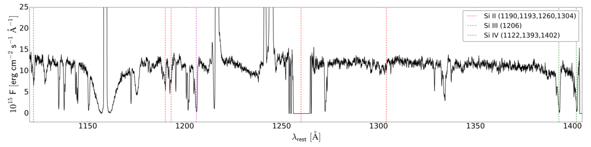
Figure 2: Cutout of the reduced COS spectrum showing the relevant metal absorption lines of Si II and Si IV. Note that the Si II absorption line at 1260Å falls into the gap between the detector segments A and B.

2.2 HST Imaging

Tol1247 was imaged with the HST in the optical using the Wide Field Ultraviolet-Visible Channel (UVIS) of its Wide Field Camera 3 (WFC3). For UV imaging the Advanced Camera for Surveys’ Solar Blind Channel (ACS/SBC) was used. Seven filters were utilized in total, allowing to apply LaXs – the Lyman alpha eXtraction software (Hayes et al., 2009) – to produce continuum-subtracted Ly$\upalpha$, H$\upalpha$ and H$\upbeta$ images, corrected for underlying stellar absorption and contamination from [N II]$\uplambda 6548,6584$. The latter one is based on the spectroscopic line ratio $\nicefrac{{[N\,II]}}{{H\upalpha}}=0.0605$ published by Terlevich et al. (1993). The imaging strategy and data reduction methodology for Tol1247 is very similar to that of the Lyman Alpha Reference Sample (LARS; Hayes et al. (2014); Östlin et al. (2014); Duval et al. (2015)) and the basic data reduction for this data set is done in the same way as for LARS. Flatfield-corrected frames were obtained from the Mikulski Archive for Space Telescope. The Charge Transfer Inefficiency (CTE) correction for the ACS data was performed by the pipeline, whereas CTE losses in WFC3/UVIS (Anderson & Bedin, 2010) were treated manually using the tools supplied by STScI. We then stacked the individual data frames and drizzled them to a pixel scale of 0.04 arcsec/px using DrizzlePac version 1.1.16 (Gonzaga et al., 2012). Further pre-processing of the data includes additional masking of cosmic rays in the drizzled frames and matching the point spread functions (PSFs) for the different filters. In order to match the PSF, we first construct PSF models for all of the filters used in the study. For the optical filters we use TinyTim models (Krist et al., 2011), resampled to a pixel scale of 0.04 arcsec/px. However, for the FUV filters TinyTim is not accurate enough, in particular in the wings. Therefore, the PSF models for the FUV filters are instead built from stacks of stars obtained in calibration observations; see Hayes et al. (2016) for details. All of the PSF models are then normalized by peak flux and stacked by maximum pixel value. We then proceed to calculate convolution kernels that match the PSFs for all of the filters to the maximum width model. Each kernel is built up from a set of delta functions and we find the optimum matching kernel by least squares optimization; see also Becker et al. (2012) and Melinder et al. (in prep). The drizzled and registered images are convolved with the kernel found for each filter, which result in a set of images matched to a common PSF.

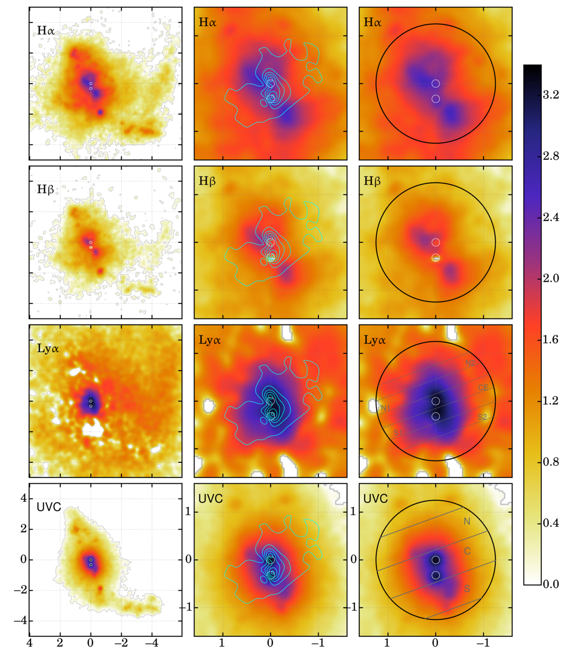
Figure 3: Results from HST imaging. North is up, east is left, with relative coordinates in arcsec. Images shown in the left column have a field of view of 10"x10", the remaining ones are zoomed-in versions that cover the central $\sim$3"x3". The logarithmic color scale is the same for all images and ranges from 0 to $10^{3.4}$ in units of $10^{-18}erg\ s^{-1}\ cm^{-2}$ for H$\upalpha$, H$\upbeta$, Ly$\upalpha$ and units of $10^{-19}erg\ s^{-1}\ cm^{-2}\ \AA^{-1}$ for the UV continuum (UVC). The black circle has a diameter of 2.5 arcsec, the size of the COS aperture, corresponding to 2.6 kpc. The cyan contours show the (smoothed) line ratio of $\nicefrac{{Ly\upalpha_{obs}}}{{H\upalpha_{0}}}$ with $H\upalpha_{0}$, the extinction corrected line flux. Thus, they trace regions of increasing Ly$\upalpha$ escape fractions. Contour levels are: 0.5, 1.5, 2.5, 3.5, 4.5 and 5.5 – corresponding to escape fractions between roughly 5 and 55%. The positions of the two clusters as seen in the UV are overplotted as white circles. The Ly$\upalpha$ and UVC images in the right column further show individual spectral extraction regions (the position angle of the COS PSA was -20^∘).

2.3 Lyman alpha eXtraction software

A galaxy’s spectral energy distribution (SED) can be understood as the sum of contributions from different components: a starburst (current episode of star formation), an underlying old stellar population (field stars) and nebular emission (continuum and lines). In this study, we make use of LaXs (Hayes et al., 2009), the Lyman alpha eXtraction software, which builds up upon the Starburst99 (Leitherer et al., 1999) spectral evolutionary models. As input for the models we assume a Kroupa IMF (Kroupa, 2001) and a SMC extinction law. The models are then constrained through SED fitting using data from our HST imaging in on-line and off-line filters. As a result, stellar ages, the star-formation history, extinction E(B-V) and the ionizing flux could be derived for each pixel.

Continuum subtraction plays a critical role and is performed using a dimensionless quantity, the continuum throughput normalization (CTN), to scale the raw count rate of the observed continuum flux (off-line) to that expected in the on-line filter. Thus, CTN is the only quantity needed when performing continuum subtraction. However, it cannot be estimated without some knowledge of the continuum itself. As shown in Hayes et al. (2005), degeneracies such as the one between age and extinction, can be resolved using (at least) four HST broadband (off-line) filters, chosen to sample the UV slope $\upbeta$, which is sensitive to both age and dust, as well as the Balmer break at 4000 Å, that is primarily sensitive to the age of the stellar population.

Based on the constrained starburst population, LaXs also creates a map of the intrinsic flux density at 900 Å from which the expected average flux density within apertures of varying sizes centered on the position of the COS aperture could be derived. The LyC escape fraction (see section 3.1) is then defined as the ratio between the predicted and observed flux density at 900 Å.

2.4 VLA Data

Tol1247 was observed at 1.4 GHz with the Karl G. Jansky Very Large Array (VLA) under program 14B-194 in September 2014 aiming to quantify the atomic gas mass of the galaxy. The VLA was operated with all 27 antennas in a hybrid DnC configuration, in which the north arm antennas are deployed in the next larger configuration than the SE and SW arm antennas. The hybrid configuration was chosen, because of the low source declination of -23^∘, for which the extended northern arm results in a more circular shaped synthesized beam. The total observing time was roughly 6 hours including overhead. For phase calibration, J1248-1959 was observed regularly and the flux density scale was fixed by observing one standard NRAO flux calibrator, 1331+305 (3C286), for which the standard NRAO flux density of $\approx 15.5$ Jy was employed. The measurement sets were checked for bad baselines which were subsequently flagged, before self-calibration was performed with CASA 4.2.2 using (E)VLA pipeline scripts. For imaging, we experimented with different levels of cleaning using CASA’s interactive mode. The cleaning threshold was found after the flux densities of unresolved sources did not further change. Uniform, natural and Briggs baseline weighting was applied to check sensitivity levels. Additional uv-tapering circularized the synthesized beam, but did not improve the sensitivity. Finally, the best result was found for natural weights without uv-tapering (see Figure 4). The synthesized beam size is 45"x36" with a position angle of 74 degree.

To measure the flux density at 1.4 GHz, we fit a 2D Gaussian to the collapsed continuum image as seen in left panel of Figure 4 using CASA’s task imfit. The flux density is then derived from the model (Gauss) shown in Figure 5. We perform the same task on two other nearby sources, NVSS J125030-233323 and NVSS J125001-233210 to check our results against previously published values from Condon et al. (1998) and find good agreement (see Table 2).

	S1.4GHz [mJy]	S1.4GHz [mJy]
	(this work)	(Condon et al. 1998)
Tololo 1247-232	4.57$\pm$0.25	3.4$\pm$0.5
J125030-233323†	72.61$\pm$0.74	69.9$\pm$2.8
J125001-233210	5.64$\pm$0.42 mJy	4.6$\pm$0.5

Table 2: Continuum flux density measured for Tololo 1247-232 and two other sources in the field. The results are in agreement with previously published values of Condon et al. (1998). †A 2-component Gauss fit was performed for J125030-233323.

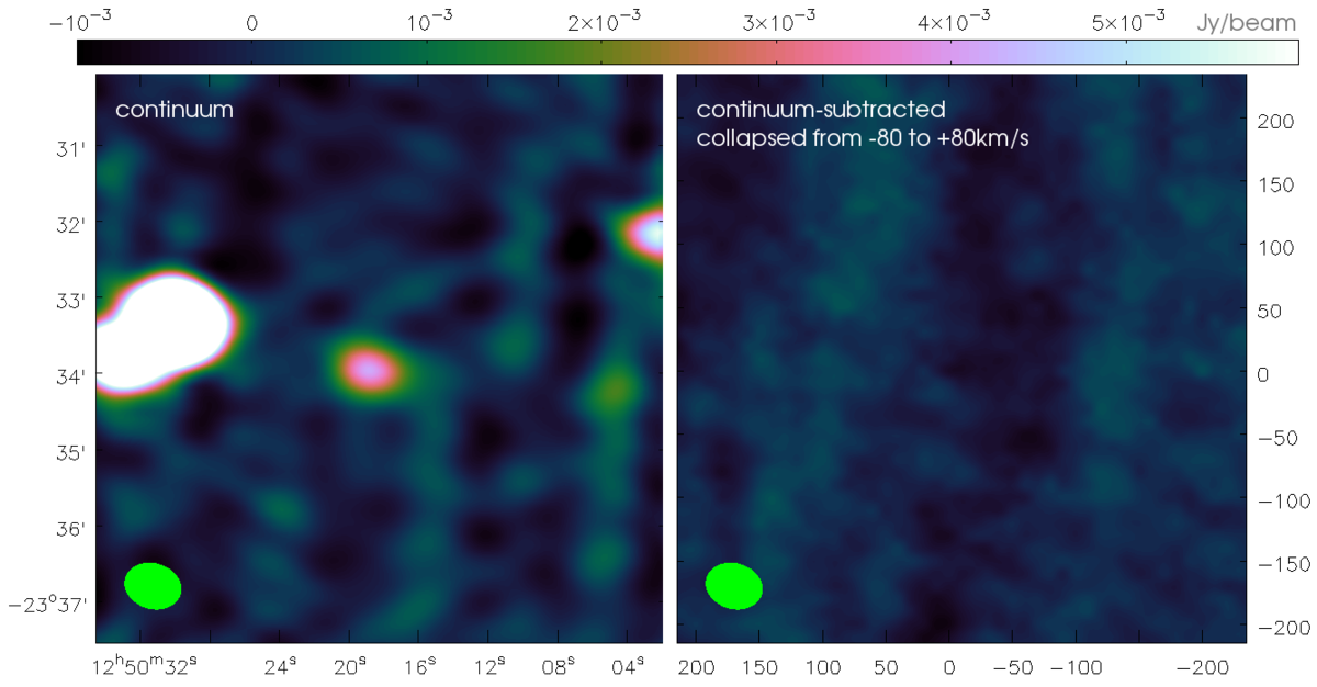
Figure 4: Cutout of the VLA 1.4 GHz image. The continuum subtraction was performed using CASA’s task imcontsub. Tololo 1247-232 is seen in the continuum (left panel) as unresolved source in the center of the image. The two nearby sources are NVSS J125030-233323 and J125001-233210 to its left and right respectively. The synthesized beam size of 45"x36" is shown in the lower left corner as green ellipse. The hydrogen 21 cm line was not detected. After fitting a 0-order polynomial to the continuum at each pixel and collapsing the spectrum from -80 to +80 km/s relative the nominal position of the line, only noise is left (right panel).

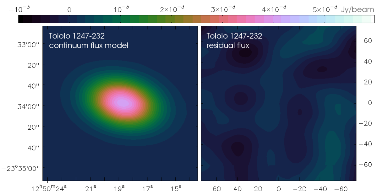
Figure 5: 2D Gaussian continuum flux density model of Tololo 1247-232 (left) and residual (right) after subtracting the model from the collapsed continuum image.

3 Results

3.1 Lyman Continuum Emission in the HST/COS spectrum

Using the individual data reduction steps as described in section 2.1, we could gradually decrease the noise level, in particular in the LyC part of the spectrum below 912Å rest-frame. However, using the CALCOS standard extraction size of 63 pixel (corresponding to the 2.5 arcsec PSA or 2.6 kpc), no significant LyC leakage could be detected at first.

We also investigate the impact of Milky Way Ly$\updelta$ absorption on our LyC spectrum. To do so, we first measure the Ly$\upalpha$ equivalent width ($\sim$14Å). Using the square root part of the “Curve of Growth”, we derive a hydrogen column density of $\sim 3.66\times 10^{20}\ cm^{-2}$, which translates into a Ly$\updelta$ equivalent width of $\sim 0.41\AA$. Thus, Ly$\delta$ Milky Way absorption has a negligible influence on our measurement.

Since LyC photons are mainly produced by massive clusters – which are known from the ACS/SBC imaging to be extremely compact – one expects LyC leakage mainly along the line-of-sight to these. Hence, the LyC signal is most likely diluted as averaging over all extracted pixel rows is done. For that reason, spectral extractions with decreasing aperture sizes were performed, in expectation of an increase in signal-to-noise ratio (SNR) with a decreasing extraction size. Figure 6 shows the resulting spectrum of the LyC part when using the nominal extraction height of 63 px as well as an extraction height of 30 px around the center, corresponding to $\sim$2.5arcsec (2.6 kpc) and $\sim$1.2arcsec (1.3 kpc) respectively. As shown in Figure 7, we have also extracted spectra using a height of only 16px (which is 0.3 arcsec or 0.3 kpc), positioned northwards, central and southwards of the two main stellar clusters (see regions N,C,S in the UVC image of Figure 3). It is found that smaller extraction regions centered around the stellar clusters indeed lead to a significant increase of the SNR in the LyC, measured between 875 and 911 Å rest-frame. Table 3 summarizes all our LyC flux measurements.

Note that the noise levels (red curves in Figure 6 and 7) are extracted from a combined dark frame that was processed in exactly the same manner as the science frame, i.e. a superdark-corrected dark image (pure noise). That way, the typical dark noise level along the spectral extraction region could be estimated.

The typical $\pm\upsigma$ noise levels shown in Figures 6 and 7 as red dashed lines, are calculated from the standard deviation of the dark noise (rms_dark) when binned to 0.5Å only. Since the observed mean flux of the Lyman continuum, <LyC>_obs, is measured over a wavelength range between 875 and 911 Å rest-frame, and thus covering more than 70 bins, we calculate the resulting SNR, assuming the dark noise is purely random:

$$SNR=\frac{<LyC>_{obs}}{\nicefrac{{rms_{dark}}}{{\sqrt{bins}}}}$$ (1)

extraction	offset	region	<LyC>obs	Unc(<LyC>obs)	SNR	<LyC>predicted	† fesc,LyC
height	from center	name					[%]
16	13	N	-0.066	0.036	-2.6	0.9	<4.0
16	-19	S	-0.201	0.039	-3.0	0.9	<4.3
16	-3	C	0.247	0.045	3.6	12.5	2.0$\pm$0.4
63	0		0.122	0.089	-0.5	21.3	<0.4
30	0		0.172	0.041	6.2	17.0	1.0$\pm$0.2

Table 3: Observed and predicted LyC flux densities in units of 10^-15 erg/s/cm²/Å for all spectra shown in Figures 6 and 7. The SNR is calculated as given by Equation (1). Using ionizing flux densities predicted through LaXs, the absolute LyC escape fractions f_esc were calculated. ^† Our result contrast those of Leitherer et al. (2016), who find a total LyC escape fraction of 4.5$\pm$1.2%. We find that the discrepancy is related to a negative flux issue that might occur at very low countrates when using CALCOS 2.21d (see also appendix A).

Table 3 shows that the SNR indeed increases when smaller apertures are used, with the highest SNRs and LyC escape fractions measured for central apertures of 30 and 16px. Since the SNR is calculated under the assumption of purely random noise (which is most likely not true), the 1$\upsigma$ errors on the derived escape fractions are only lower limits on the real error. We conclude that the LyC escape fraction of Tol1247 is 1.5$\pm$0.5% only.

Our result contrast those of Leitherer et al. (2016), who find a LyC escape fraction of 4.5$\pm$1.2%. We find that the discrepancy is related to a negative flux issue that might occur at very low countrates when using CALCOS 2.21d (see also appendix A).

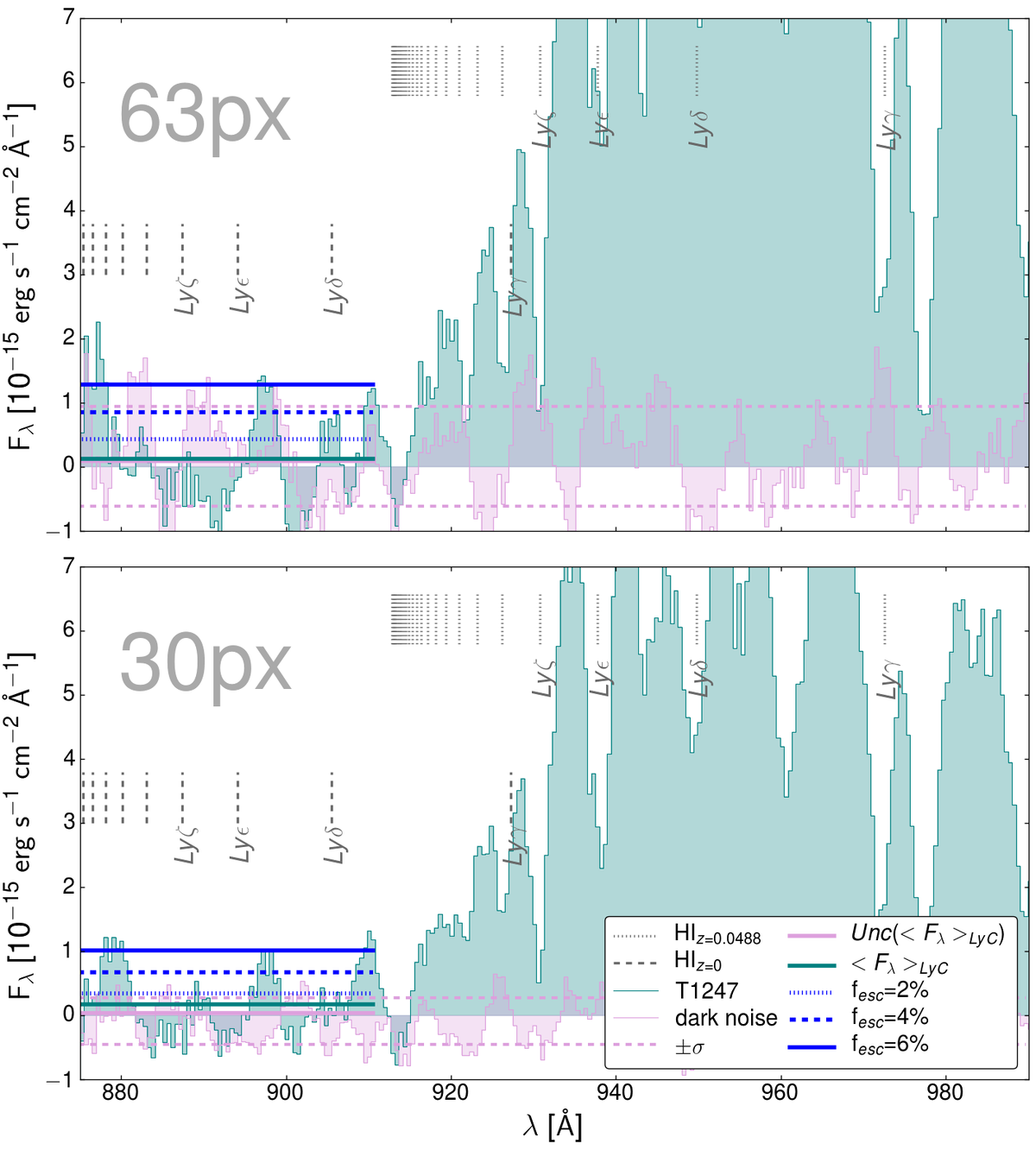
Figure 6: Spectral extractions of the rest-frame Lyman continuum part using the modified CALCOS pipeline. The spectra are extractions with apertures of 63 (top panel) and 30 pixel (bottom panel). Green bins show the signal of Tol1247 and red bins are extractions from a combined dark frame that was processed in exactly the same manner as the science frame, i.e. a superdark-corrected dark image (pure noise). That way, the typical dark noise level along the spectral extraction region could be estimated. The green horizontal line shows the mean flux level of the signal (Tol1247) in the range 875–911 Å. The red horizontal line is the same for the dark noise level (which should be close to zero). The blue horizontal lines indicate limits for the LyC escape fraction of 6% (blue solid line), 4% (blue dashed line) and 2% (blue dotted line). The Lyman series and limits are shown for Tol1247 and the airglow as dotted and dashed vertical lines respectively.

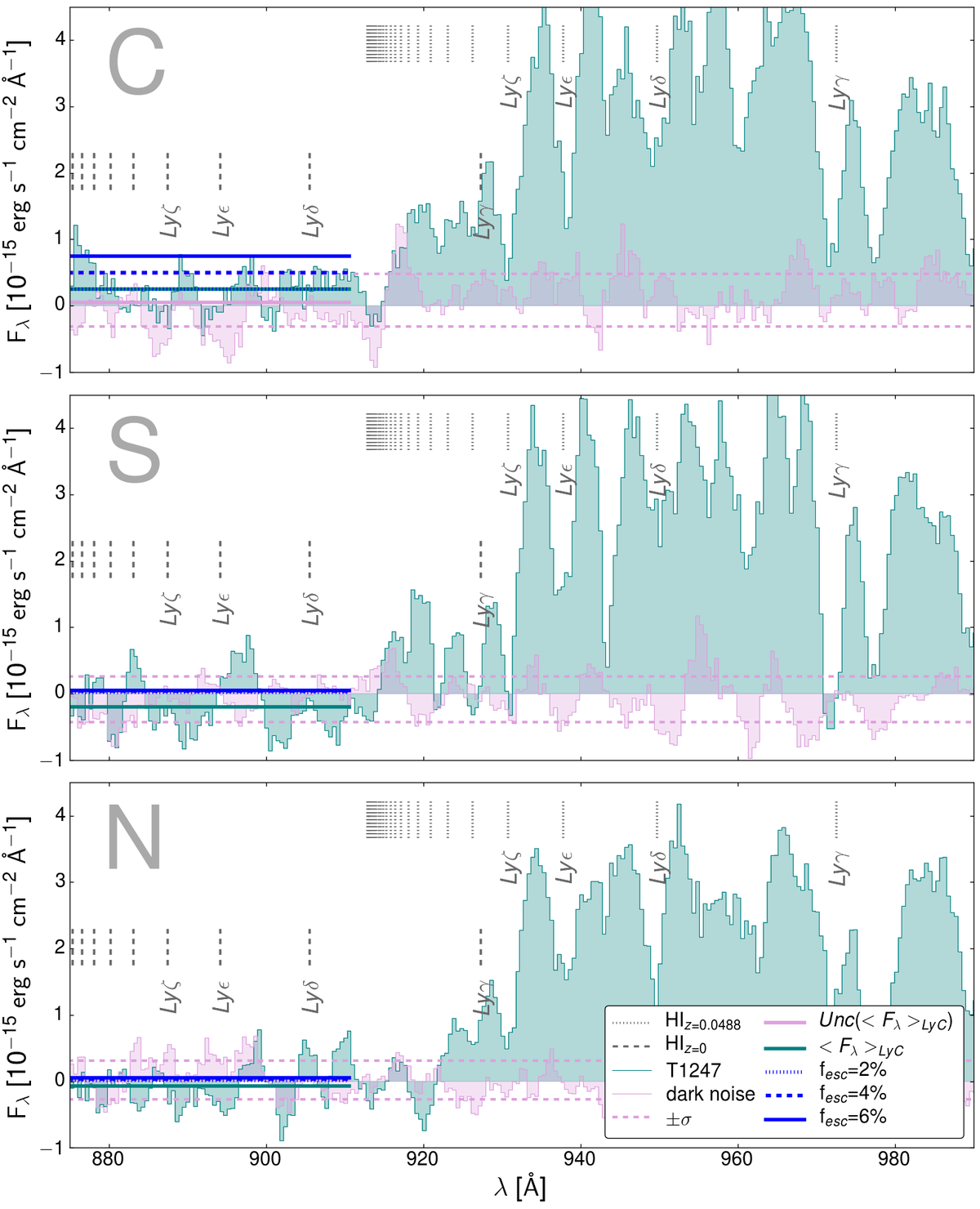
Figure 7: Same as Figure 7, but for extraction heights of 16 pixel, centered on offset positions as shown in Figure 3.

3.2 Constraints from UV Absorption Lines

Our COS spectra cover a multitude of UV absorption lines (see Figure 2). In order to study bulk motions of the gas, we place all lines on a common velocity grid and create inverse variance weighted average spectra tracing the neutral and ionized gas respectively. We use the Si II transitions with ionization potentials below 1 Rydberg at $\uplambda\uplambda$ 1190,1193 Å (CENWAVE=1327, segment B), $\uplambda\uplambda$ 1304 Å (CENWAVE=1327, segment A), along with transitions of O I at $\uplambda\uplambda$ 1302 Å and C II at $\uplambda\uplambda$ 1334 Å to trace kinematics of the neutral medium. The Si IV lines at $\uplambda\uplambda$ 1122 Å (CENWAVE=1327, segment B) and $\uplambda\uplambda$ 1393,1402 Å (CENWAVE=1327, segment A) were used as ionized gas tracer.

We calculate velocity parameters as defined by Rivera-Thorsen et al. (2015), who derived the same quantities for the Lyman Alpha Reference Sample (LARS; Hayes et al. (2013, 2014); Östlin et al. (2014)). A summary of all derived quantities is shown in Table 4. As Figure 8 shows, the linewidth $W(90\%)$ – defined as the distance on the velocity axis from 5% to 95% integrated absorption – is very wide with a value of 559 km/s and the gas moves very fast, at a line-of-sight integrated central velocity v_int of -190 km/s – the velocity which has 50% of the integrated absorption on each side. Compared to the 14 LARS galaxies, Tol1247’s values of W(90%) and v_int are found among the extremes, slightly superseded only by two LARS galaxies.

Although most of the gas absorption is blueshifted, also gas moving at positive velocities is seen and in particular a sharp rise towards 0-velocity can be identified. This behavior is very similar to the findings of Rivera-Thorsen et al. (2015). However, with a velocity v_95% of -506 km/s – the absolute value of the velocity which has 95% of the integrated absorption on its red side – Tol1247 even outstands all of the LARS galaxies. This indicates that very strong feedback processes are at work in Tol1247 that accelerate the ISM. This facilitates the escape of Ly$\upalpha$ photons through superwinds, resembling the findings of Duval et al. (2015).

A comparison of the mean low-ionization (LIS) absorption profile and Si IV in Figure 9 shows that the low and high ionization lines are very similar in their structure, e.g. both share an absorption bump at $\sim-450$ km/s. However, Si IV absorption is stronger with a minimum relative flux $\nicefrac{{I}}{{I_{0}}}_{min}$ of only $\sim$0.2 at $\sim-100$ km/s. This suggests that most of the gas in the observed medium is highly ionized, increasing the probability for LyC photons to escape, e.g. through density bounded regions.

parameter	value	comment
$\nicefrac{{I}}{{I_{0}}}_{0}$	0.84$\pm$0.15	relative flux at v=0
$\nicefrac{{I}}{{I_{0}}}_{min}$	0.60$\pm$0.07	minimum relative flux
$W(90\%)$	559.8$\pm$0.1 km/s	linewidth from 5 to 95%
		integrated absorption
$v_{95\%}$	-506.2$\pm$0.1 km/s	velocity which has 95% of
		absorption on its red side
$v_{int}$	-190.4$\pm$0.1 km/s	velocity which has 50% of
		absorption on each side
$v_{min}$	-61$\pm$111 km/s	velocity at minimum
		relative flux

Table 4: Quantities derived from the average low ionization line profile as seen in Figure 8.

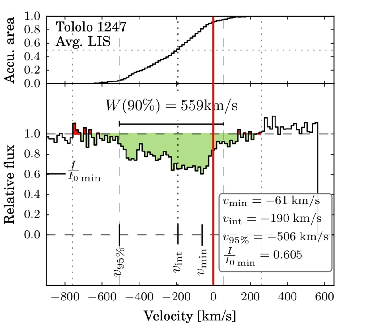
Figure 8: Mean low-ionization (LIS) line profile (containing Si II, O I and C II) with velocity parameters as defined by Rivera-Thorsen et al. (2015), where v_int is the velocity which has 50% of the integrated absorption on each side, v_95% is the absolute value of the velocity which has 95% of the integrated absorption on its red side and v_min is the velocity at the minimum intensity, i.e. bulk of the gas moves with a velocity v_min.

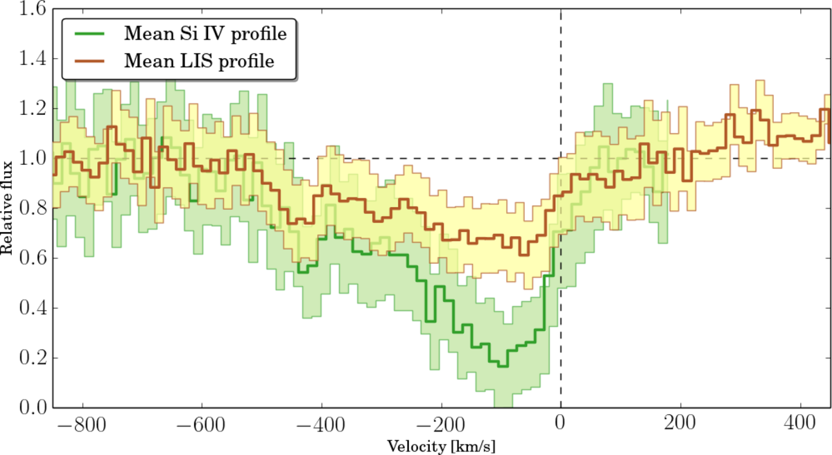
Figure 9: Comparison of the mean low-ionization (LIS) line profile (containing Si II, O I and C II) and the mean Si IV absorption profile. The overall trend is similar for both, the neutral and ionized medium traced by the LIS and Si IV profile respectively. However, bulk of the gas along the line-of-sight is highly ionized, supporting LyC leakage in case of density bound regions.

3.3 Covering Fraction and Column Density

Next, we make use of the apparent optical depth method as described by Savage & Sembach (1991), used by Pettini et al. (2002), Quider et al. (2009) and more recently applied by Jones et al. (2013) and Rivera-Thorsen et al. (2015), allowing to compute the column density N_SiII and covering fraction f_c of these lines as a function of velocity offset from the systemic zero-point (see Figure 10). The method utilizes the fact that the absorption depth of transitions from the same ground state, in the case of an optical thin medium depend on the product of oscillator strength and wavelength $f\uplambda$, whereas an optical thick medium with partial covering will yield identical absorption features in all transitions. The ratio of the residual intensity I to the continuum I₀ within a given velocity interval is utilized to calculate the covering fraction f_c and the optical depth $\tau$:

$$\frac{I}{I_{0}}\ =\ 1\ -\ f_{c}\ (1\ -\ e^{-\tau})$$ (2)

The optical depth $\tau$ is further related to column density N_SiII and the oscillator strength $f$ via

$$\tau=f\uplambda\ \frac{\uppi e^{2}}{m_{e}c}\ N_{SiII}\ =\ f\uplambda\ \frac{N_{SiII}}{3.768\ \times\ 10^{14}},$$ (3)

with the wavelength $\uplambda$ in Å and N_SiII in $cm^{-2}$. Since we observed multiple Si lines that arise from the same energy level, but have different values of $f\lambda$, a minimizing routine could be formulated to find solutions for N_SiII and $f_{c}$. Practically, a grid of (N_SiII, $f_{c}$) pairs was defined and limited by physically sensible values only. The squared residuals of subtracting the measured value of the ratio I/I₀ from the one found at the grid point, could then be calculated and minimized. We refer to Rivera-Thorsen et al. (2015) for a detailed description of the applied method.

Similar to the LARS galaxies, also Tol1247 shows no or little dependency of $f\uplambda$ on the absorption depth of the considered silicon lines. Thus, the medium must be optically thick, but clumpy since strong residual flux is seen at all velocities with a minimum value (maximum covering) of $\nicefrac{{I}}{{I_{0}}}_{min}$ of $\sim$0.35. The derived covering fraction as seen in right panel of Figure 10 shows that even the maximum value for f_c is low with a value of $\sim$0.7. Note that f_c basically follows the absorption feature. For some of the spectral bins however, the derived errors of the fitting procedure are spanning over the entire range of physical values, indicating that no unique solution could be found. This is due to the non-linear solution characteristics of the applied method. From the observed low covering fraction, one might expect Ly$\upalpha$ emission at line center. However this is not observed (see Figure 11), suggesting that an additional somewhat diffuse component of H I exists with a lower column density that may instead absorb the Ly$\upalpha$ radiation. Such low column density gas would still re-shape the Ly$\upalpha$ line without leaving an observable imprint in the silicon absorption lines. Hence, we now investigate whether our observations are still consistent with the presence of such a gas component, in particular at the systemic velocity, where we find that the Si II column density is lowest with an lower limit of only $\sim 10^{11.3}\ cm^{-2}$ (see third panel of Figure 10). The metallicity of Tol1247 is 12+log(O/H)=8.1 (Terlevich et al., 1993) or 1/4 Z_⊙. Thus, the Si II column density can be converted into a H I column density of $\sim 2.3\ \times\ 10^{16}\ cm^{-2}$ assuming 12+log(Si/H)_⊙=7.55  as given in Lequeux (2005) and that all Si in the neutral medium is in form of Si II. This is indeed less than the typical value of $1.6\ \times\ 10^{17}\ cm^{-2}$ (Mo et al., 2010) for Lyman Limit Systems (LLS), supporting the escape of ionizing photons from the central region, which is assumed to be co-spatial with the gas seen in absorption at systemic velocity. At the same time, this is $\sim$10⁴ optical depths for Ly$\upalpha$, hence absolutely optically thick to Ly$\upalpha$. The presence of an additional diffuse component thus might explain the lack of Ly$\upalpha$ flux at the systemic velocity, in a system that at the same time leaks ionizing photons. Farther out at a typical velocity $v_{min}$ at which bulk of the gas moves, the column density of Si II is set to $\sim 10^{12.5}\ cm^{-2}$, which translates into a hydrogen column density of $3.6\ \times\ 10^{17}\ cm^{-2}$. Although still low, this is optically thick to both LyC and Ly$\upalpha$. Thus, LyC likely escapes due to the combined effect of low gas column at systemic velocity (similar to a central cavity) and the interstellar medium being clumpy, i.e. channels through which LyC can escape from the galaxy.

We further examine the overall N_SiII sensitivity limit per velocity bin of our observations, which can be identified through the error bars in Figure 10. We see that the relative flux sensitivity is $\sim 0.1$, so that for total covering (diffuse medium): $\nicefrac{{I}}{{I_{0}}}=e^{-\uptau}=0.9$. With the relation between the optical depth and column density (see Equation 3), and an average product of wavelength and oscillator strength of f$\uplambda$=384.8 for the given average spectrum, a Si II column density of N=$1.0\ \times\ 10^{11}\ cm^{-2}$ is found, describing the sensitivity limit of our observations. As above, this translates into a hydrogen column density of $1.1\ \times\ 10^{16}\ cm^{-2}$, which is still optically thick to Ly$\upalpha$, but optically thin by at least one magnitude to Lyman continuum; compare Verhamme et al. (2015). In agreement with the observations, we thus conclude that the observed medium is clumpy with optically thick clouds that are partially covering. Additionally, a more diffuse component or inter-clump medium may be present that is optically thick to Ly$\upalpha$, but provides at least one clear sightline for Lyman continuum to leak.

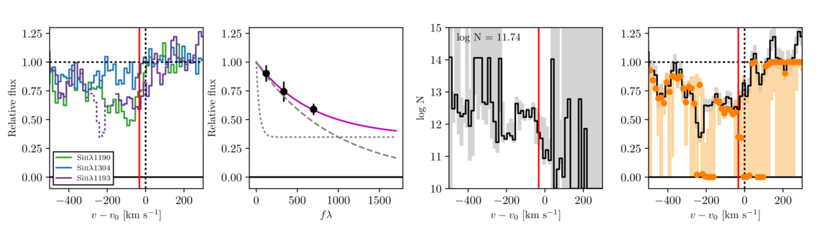
Figure 10: Explanation of the apparent optical depth method as described in Rivera-Thorsen et al. (2015) and Rivera-Thorsen et al. (2017). Left panel: The Si II lines utilized to solve for the column density and covering fraction (blended regions are drawn as dashed lines). For one velocity bin (marked with red line), the three measured relative intensities are shown in the second panel as black markers in the f$\uplambda$ vs. I/I₀ plane. The best-fit function that finally leads to the column density and covering fraction is drawn in magenta. The solutions for N_SiII and the covering fraction are shown in the third and last panel respectively.

3.4 Lyman Alpha Emission Line Spectrum

The Ly$\upalpha$ profile in Figure 11 shows extractions along the x-dispersion around the central region of the COS aperture. Note that in this setup (CENWAVE=1327Å) the nominal spectral extraction height which corresponds to the 2.5 arcsec PSA is 35 pixel only. We have performed four pixel wide extractions, i.e. covering $\sim$0.29 arcsec, at positions of -8, -4, 0, +4 and +8 px offset from the PSA center (see also Figure 3). Hence, we extract regions ranging from 0.58 arcsec North which is one quarter above (turquoise lines in Figure 11) to 0.58 arcsec South which is one quarter (violet lines) below the center of the COS aperture. No obvious line shift can be deduced from the extractions, suggesting that both central clusters create a common expanding gas shell.

The emission line shows a characteristic P-Cygni profile (Kunth et al., 1998; Wofford et al., 2013; Rivera-Thorsen et al., 2015), with weak emission at the blue side. Interestingly, the strongest metal absorption coincides with the Ly$\upalpha$ trough (compare Figures 11 and 9), probably meaning that the gas that absorbs most of the metals, also provides much of the absorption in Ly$\upalpha$.

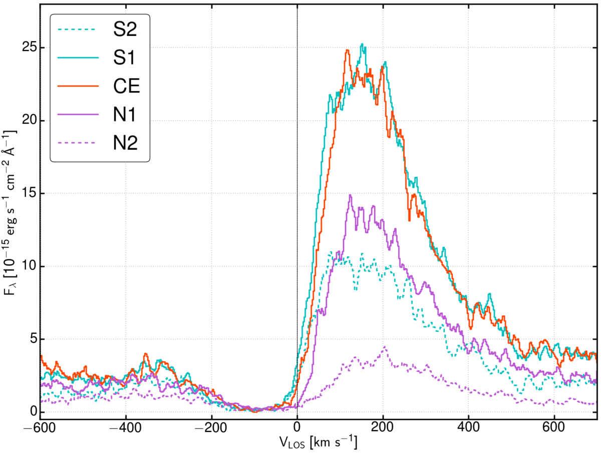
Figure 11: Lyman Alpha emission line profile extracted from North one quarter above (turquoise lines) to South one quarter (violet lines) below the center of the COS aperture. No obvious line shift can be deduced from the extractions. No flux is seen at systemic velocity, taking into the account the uncertainty of the measured redshift ($\pm$0.0002).

3.5 Radial Surface Brightness Profile

At the given distance to Tol1247, the pixel scale of 0.04 arcsec/px in Figure 3 corresponds to 42 parsec per pixel. At this scale, complex structures can be revealed. The H$\upalpha$ map shows an overall bar-like distribution with individual clumps of strong emission – likely associated with massive stellar clusters – along its main axis and an increasingly filamentary structure towards the outer regions. In particular, an arc with a diameter of roughly 300 pc can be identified associated with the most luminous cluster close to the center, indicative for a highly turbulent ionized medium or outflows.

The radial surface brightness profile in Figure 12 shows that the Ly$\upalpha$ emission is strongest in the central region, however with a steep decline up to a radius of $\sim$1 kpc. This is interesting, because such behavior may be explained by a low column density or significant ISM clumping, i.e. less Ly$\upalpha$ scattering and a compact emission of Ly$\upalpha$. Thus, we find another indication for LyC to escape directly. Farther out, the Ly$\upalpha$ profile flattens and its surface brightness is less than the one in H$\upalpha$ up to a radius of $\sim$3 kpc. At this point, the medium starts changing from mostly ionized to mostly neutral, until at $\sim$5.2 kpc no significant H$\upalpha$ emission is observed anymore. However, Ly$\upalpha$ is seen up to $\sim$6.2 kpc in form of a halo. The latter one is likely produced due to the clumpyness of the ISM in combination with strong ionizing flux emerging from the central clusters that is converted to Ly$\upalpha$ that resonantly scatters outwards. Due to the clumpyness the effect of the dust on the Ly$\upalpha$ line profile is less efficient than in homogeneous media, causing an intense Ly$\upalpha$ emission that can escape even from a very dusty clumpy ISM (Scarlata et al., 2009; Duval et al., 2015).

3.6 Extinction

The Galactic dust reddening towards Tol1247 is $E(B-V)=0.075$ mag or $A_{V}$=0.23 mag (Schlafly & Finkbeiner, 2011). Note that all observational fluxes reported are already corrected for the Galactic reddening and all $A_{V}$ values only account for the intrinsic attenuation within Tol1247. Attenuation due to dust within Tol1247 was calculated from the Balmer decrement using the Cardelli et al. (1989) (CCM) attenuation law for the Milky Way (MW) and the Calzetti et al. (2000) one for starbursts (SB). An intrinsic, theoretical $\nicefrac{{H\upalpha}}{{H\upbeta}}$ ratio of 2.80 was calculated for an electron temperature of 12100 K, which was published by Terlevich et al. (1993) based on the [O III]$\uplambda 5007$/[O III]$\uplambda 4363$ emission line ratio. Both prescriptions give similar results for the average V-band attenuation of the galaxy, i.e. 0.47 and 0.53 mag $A_{V}$ (see Figure 13) for MW and SB laws. Within the COS aperture, the average attenuation $A_{V}$ is 0.43 and 0.49 mag, respectively. Although the COS average is only slightly less than for the whole galaxy, the attenuation in the innermost $\sim 500\,pc$ is in fact much lower with $A_{V}$ down to $\sim$0.2.

Given the starburst nature of Tol1247, we use $A_{V}=0.49$ derived using the Calzetti law to estimate the average total hydrogen ($N_{H}=N_{HI}+2N_{H_{2}}+N_{HII}$) column density $N_{H}$ within the COS aperture using equation (4) taken from Güver & Özel (2009).

$$N_{H}\ =\ 2.21\ \times\ 10^{21}\ \times\ A_{V},$$ (4)

where $N_{H}$ is given in $cm^{-2}$ and $A_{V}$ in mag. Using this, a total hydrogen column density of $1.1\ \times\ 10^{21}\ cm^{-2}$ is found. However, we are mainly interested in $N_{H\,I}$, since both LyC and Ly$\upalpha$ are absorbed or scattered by the neutral atomic gas. Thus, we consider an empirically motivated range of molecular-to-atomic hydrogen ratios ($\mu$) as well as ionization fractions ($\iota$), in order to calculate lower and upper limits for $N_{H\,I}$:

$$N_{HI}\ =\ \frac{N_{H}}{1+\mu+\iota},$$ (5)

where $\mu=\nicefrac{{2N_{H_{2}}}}{{N_{HI}}}$ and $\iota=\nicefrac{{N_{HII}}}{{N_{HI}}}$. For the upper limit atomic hydrogen column density we adopt $\mu=\nicefrac{{1}}{{5}}$, which is lower than the value that is typically found in most present-day galaxies ($\nicefrac{{1}}{{3}}$). We have chosen this value based on the results of the COLD GASS survey (Saintonge et al., 2011a, b; Kauffmann et al., 2012), which revealed that bluer galaxies tend to have lower molecular gas fractions.

Support for a lower molecular gas fraction in starbursts is also found by e.g. Amorín et al. (2016), who studied gas fractions and depletion times in a sample of $\sim 20$ low-metallicity starbursts (blue compact dwarf galaxies), accounting for a metallicity-dependent CO-to-H₂ conversion factor. However, huge uncertainties remain, and the contrary seems to be found in e.g. Haro 11 (Pardy et al., 2016). We further assume that only half of the hydrogen atoms are ionized ($\iota=1$), although our deep Si IV absorption profile gives rise to an even higher ionization fraction. That way, we find an upper limit $N_{HI}<4.9\ \times\ 10^{20}\ cm^{-2}$. To derive a lower atomic hydrogen column density we adopt $\mu=3$ and $\iota=3$, again most likely overshooting the true value and we find a lower limit $N_{HI}>1.6\ \times\ 10^{20}\ cm^{-2}$. Even the lower limit is $\sim 10^{3}$ optical depths for LyC photons, but as explained before in the central region LyC photons could still escape through channels in the clumpy ISM.

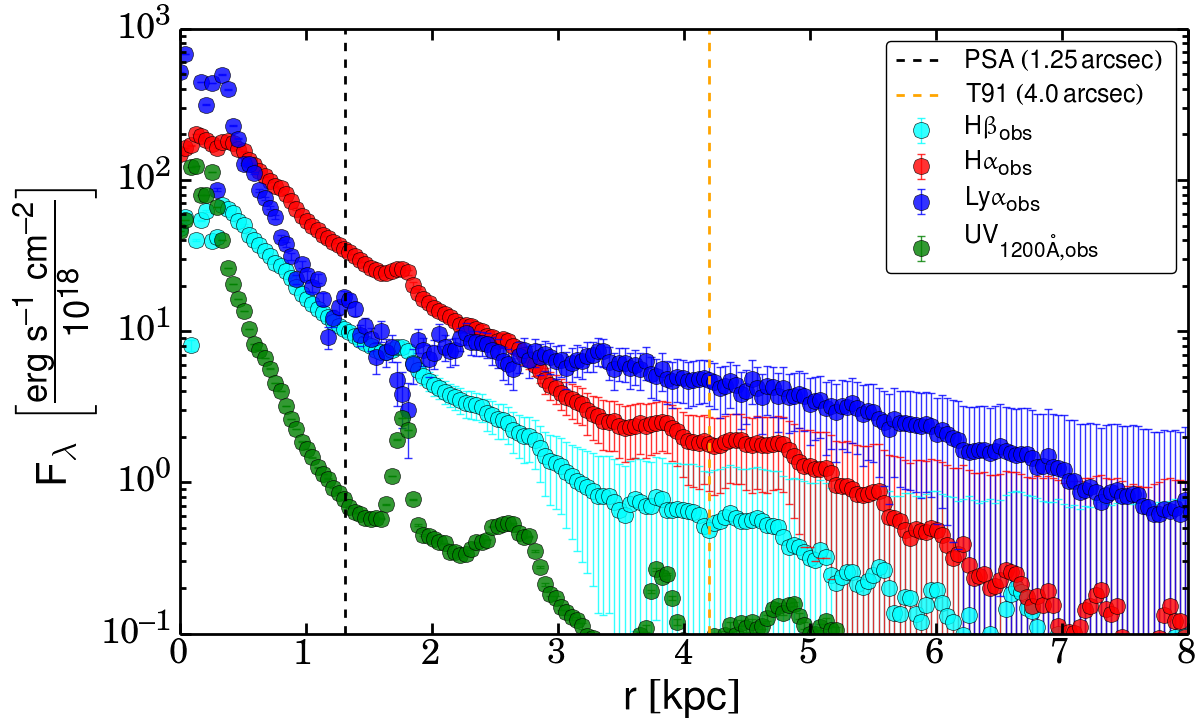
Figure 12: Mean surface brightness of H$\upalpha$, H$\upbeta$, Ly$\upalpha$ and UV continuum at $\sim$1200Å evaluated from the center of the COS aperture outwards in steps of one pixel at a pixel scale of 0.04 arcsec/px, corresponding to 42 pc/px. The vertical black dashed line indicates the radius covered by the COS aperture and the vertical orange dashed line shows the limit of the (rectangular) aperture that was used by Terlevich et al. (1991).

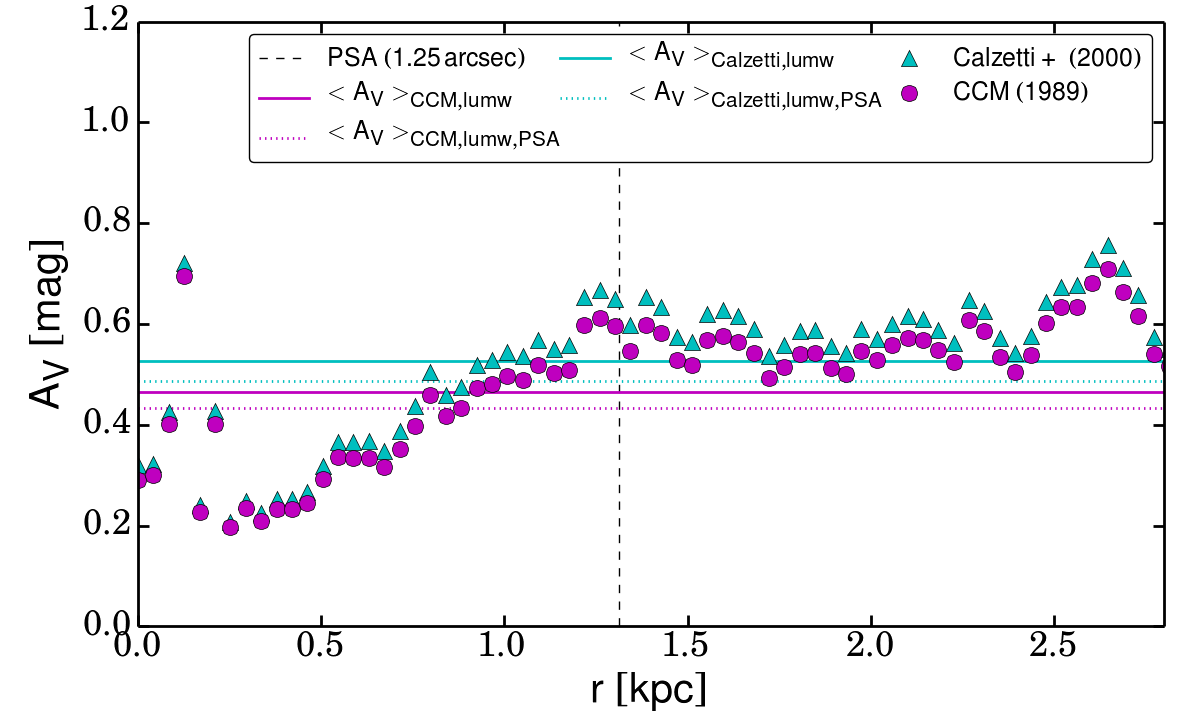
Figure 13: Average radial luminosity-weighted V-band attenuation within Tol1247 using the Cardelli et al. (1989) (magenta) and Calzetti et al. (2000) law (cyan). $A_{V}$ is evaluated from the center of the COS aperture outwards in annuli of one pixel at a pixel scale of 0.04 arcsec/px, corresponding to 42 pc/px. The vertical black dashed line indicates the radius covered by the COS aperture. Horizontal solid lines are set at the average luminosity-weighted attenuation found within the whole galaxy (limited by H$\upbeta$ sensitivity) and the COS aperture (dashed lines).

3.7 Total H$\upalpha$, H$\upbeta$ and Ly$\upalpha$ Flux Measurements

Using our continuum-subtracted images and accounting for Galactic extinction towards Tol1247, we calculate the total observed line fluxes for $H\upalpha$, H$\upbeta$ and Ly$\upalpha$. The $H\upalpha$ and H$\upbeta$ fluxes were further corrected for internal extinction using the Cardelli et al. (1989) and Calzetti et al. (2000) attenuation laws as described in the previous section. Our results are summarized and compared to previous findings in Table 5. Note that Terlevich et al. (1991) used an aperture of 8x8 arcsec and thus should recover bulk of the total flux of Tol1247. Indeed, our $H\upalpha$ flux is comparable to the one published by Terlevich et al. (1991), i.e. only 4% higher and thus within the uncertainty that was estimated by Terlevich et al. (1991) to be $\sim$10%. However, our total H$\upbeta$ flux is larger by $\sim$20%. Nevertheless, our extinction-corrected fluxes are still in good agreement with the ones published by Rosa-González et al. (2007) (that are based on Terlevich et al. (1991)).

Line	FluxPSA	Fluxtot	$\frac{Flux_{tot}}{Flux_{ref}}$	Ref.
(1)	(2)	(3)	(4)	(5)
H$\upalpha$	25.9$\pm$0.3	52.6$\pm$4.1	1.04	T91
H$\upbeta$	8.0$\pm$0.2	16.2$\pm$1.2	1.20	T91
Ly$\upalpha$	28.0$\pm$0.5	64.1$\pm$6.4	1.00	T93$\dagger$
H$\upalpha_{0,MW}$	36.2$\pm$0.4	75.4$\pm$6.0	0.89	RG07
H$\upbeta_{0,MW}$	12.9$\pm$0.3	27.2$\pm$1.7	0.92	RG07
H$\upalpha_{0,SB}$	37.5$\pm$0.4	78.4$\pm$6.2	0.92	RG07
H$\upbeta_{0,SB}$	13.4$\pm$0.3	28.2$\pm$1.7	0.96	RG07

Table 5: Comparison of observed emission line fluxes and previously published values. The fluxes given in the table are corrected for Galactic extinction using E(B-V)=0.075. Column 1: Line name. Column 2: Continuum-subtracted line flux in units of 10^-14 erg/s/cm² within the PSA. Column 3: Continuum-subtracted line flux in the same unit as before for the whole galaxy. Column 4: Comparison to previously published values with the reference given in Column 5:: T91: Terlevich et al. (1991), T93: Terlevich et al. (1993), RG07: Rosa-González et al. (2007). Fluxes corrected for extinction are indicated by an index $0$ followed by either MW or SB for the Milky Way or starburst attenuation law respectively. $\dagger$ The comparison here is based on a new calibration of the line flux in the IUE spectrum, that was first published by Terlevich et al. (1993).

3.8 Star Formation Rates

We calculate star formation rates (SFR) from 1.4GHz continuum as well as based on our MW and SB extinction-corrected H$\upalpha$ and UV continuum fluxes. Stellar and nebular continuum are thereby related through: $E(B-V)_{stellar}=0.44\ \times\ E(B-V)_{nebular}$ (Calzetti et al., 2000). In order to make a fair comparison between all SFRs, we use SFR calibrations based on stellar population synthesis performed by Sullivan et al. (2001), which assume a constant star formation history (SFH) and a Salpeter (1955) initial mass function (IMF) . The conversions are shown in Equations (6)–(10). Since UV and 1.4 GHz calibrations undergo a strong evolution within the first $\sim$100 Myr, we calculate SFRs for ages of 10 and 100 Myr. Our results are shown in Table 6.

$$SFR_{H\upalpha}\ =\frac{L_{H\upalpha,0}\ [erg\ s^{-1}]}{1.22\ \times\ 10^{41}}\ [M_{\odot}\ yr^{-1}]$$ (6)

$$SFR_{UV,10Myr}\ =\frac{L_{UV,0}\ [erg\ s^{-1}\ \AA^{-1}]}{3.75\ \times\ 10^{39}}\ [M_{\odot}\ yr^{-1}]$$ (7)

$$SFR_{UV,100Myr}\ =\frac{L_{UV,0}\ [erg\ s^{-1}\ \AA^{-1}]}{5.76\ \times\ 10^{39}}\ [M_{\odot}\ yr^{-1}]$$ (8)

$$SFR_{1.4GHz,10Myr}\ =\frac{L_{1.4GHz,NT}\ [erg\ s^{-1}\ Hz^{-1}]}{2.39\ \times\ 10^{27}}\ [M_{\odot}\ yr^{-1}]$$ (9)

$$SFR_{1.4GHz,100Myr}\ =\frac{L_{1.4GHz,NT}\ [erg\ s^{-1}\ Hz^{-1}]}{8.85\ \times\ 10^{27}}\ [M_{\odot}\ yr^{-1}]$$ (10)

The non-thermal luminosity $L_{1.4GHz,NT}$ at 1.4 GHz rest must be given in $erg\ s^{-1}\ Hz^{-1}$, i.e. we use our 1.4 GHz flux measurement from Table 2, convert it to cgs units and adopt a K-correction: $L_{1.4GHz,rest}\ =\ L_{1.4GHz,obs}\ \times\ (1\ +\ z)^{-\upalpha}$, using a spectral power law slope $\upalpha=-0.8$. Next, the non-thermal fraction at 1.4 GHz is estimated using equations 21 and 23 of Condon (1992): $L_{1.4GHz,rest,NT}\ =\ 0.87\ \times\ L_{1.4GHz,rest}$.

	10Myr	100Myr
SFRHα,0,MW	34.8	34.8
SFRHα,0,SB	36.2	36.2
SFRUV,0,MW	49.2	32.4
SFRUV,0,SB	46.9	30.9
SFR1.4GHz	96.2	26.0
$\nicefrac{{SFR_{H\upalpha,0,MW}}}{{SFR_{1.4GHz}}}$	0.36	1.34
$\nicefrac{{SFR_{H\upalpha,0,MW}}}{{SFR_{UV,0,MW}}}$	0.71	1.07
$\nicefrac{{SFR_{H\upalpha,0,SB}}}{{SFR_{1.4GHz}}}$	0.38	1.39
$\nicefrac{{SFR_{H\upalpha,0,SB}}}{{SFR_{UV,0,SB}}}$	0.77	1.17

Table 6: Predicted SFRs in $M_{\odot}\ yr^{-1}$ for Tol1247, based on SF tracers and calibrations by Sullivan et al. (2001), which assume a constant SFH and a Salpeter IMF. Values derived from extinction corrected fluxes are indicated by $0$. Corrections based on a Milkyway and starburst attenuation law are denoted by $MW$ and $SB$ respectively.

3.9 Lyman Alpha Escape Fraction

A typical H II region with a temperature of $\sim 10^{4}$ K and an electron density of 10${}^{3}cm^{-3}$, is optically thick for energetic photons from massive O and B stars that are able to ionize hydrogen (LyC photons: E>13.6 eV or $\uplambda$<912 Å). However, 68% (Dijkstra, 2014) of these photons are transformed into Ly$\upalpha$ radiation. This is due to the recombination process that follows the absorption of a LyC photon. In recombination theory, at least two limiting cases (A and B) can be distinguished for which – in the absence of dust – the intrinsic line intensity ratio of Ly$\upalpha$ to H$\upalpha$ is known (Osterbrock & Ferland, 2006). In case A, the medium is optically thin in all hydrogen lines including the Lyman lines. Hence, Lyman photons can freely escape, as well as the other photons from hydrogen recombination. Such a H II region is called density bounded, because the luminosity is set by the density of the medium rather than the number of photons. In case B, the medium is optically thick in all Lyman lines, but optically thin in all other hydrogen lines, which is called ionization bounded. In this scenario, Ly$\upalpha$ photons are immediately absorbed (on the spot) and thus excite another hydrogen atom that is followed by recombination and the emission of Ly$\upalpha$. This process is called resonant scattering. However, for both cases the line ratio of Ly$\upalpha$ to H$\upalpha$ ranges only from around 7 to 12 for case B and A respectively (Wofford et al., 2013). We now define a Ly$\upalpha$ escape fraction f_esc,Lyα by dividing the measured line ratio to the intrinsic one. Following Hayes (2015), for the intrinsic Ly$\upalpha$ to H$\upalpha$ ratio a value of 8.7 is commonly adopted for case B recombination. However, for Tol1247 we use an intrinsic ratio of 10, assuming that the conditions in Tol1247 are at least partly density bounded, supported by our comparison of the Si II and Si IV absorption profiles in Figure 9 and also suggested by the contour maps overplotted in Figure 3 that follow the $\nicefrac{{Ly\upalpha_{obs}}}{{H\upalpha_{0}}}$ ratio, i.e. tracing the Ly$\upalpha$ escape fraction. The contours show that the Ly$\upalpha$ escape fraction is highest slightly offset from the line-of-sight to the stellar clusters. We argue that this is due to the combined effect of a clumpy geometry and strong ionizing radiation field close to the central clusters, which results in a density bounded emission line region. Thus, we calculate the Ly$\upalpha$ escape fraction using $f_{esc,Ly\upalpha}=\nicefrac{{Ly\upalpha_{obs}}}{{(H\upalpha_{0}\ \times\ 10)}}$ with H$\upalpha_{0}$ the extinction corrected flux and find Ly$\upalpha$ escape fractions of 8.2$\pm$1.5% and 7.5$\pm 0.5$% for the whole galaxy (including the halo) and within the COS aperture only. Note that we find basically the same escape fraction for both attenuation laws (MW and SB).

3.10 Upper Limit for the atomic Gas Mass

The hydrogen hyperfinestructure line at 21 cm remained undetected in Tol1247. However with the current data, we can calculate an upper limit for the atomic gas mass. We do so by measuring the noise level in the velocity-integrated (from -80 to +80km/s), continuum-subtracted line map that is shown in the right panel of Figure 4 and find a 1$\sigma$ level of 0.28 mJy/beam. Since Tol1247 is unresolved, the corresponding flux density is 0.28 mJy. With a detection threshold of 2$\sigma$ and a typical linewidth of 160 km/s, we estimate the 21 cm velocity-integrated flux limit S₂₁ to 90 mJy km/s for Tol1247. With the widely used relation from Roberts & Haynes (1994), which is shown in equation (11), we arrive at an upper atomic mass limit of $\approx$10${}^{9}M_{\odot}$. M_HI is given in $M_{\odot}$, S₂₁ in mJy km s^-1 and D_L in Mpc.

$$M_{HI}=236\times D_{L}^{2}\times S_{21}\ [M_{\odot}]$$ (11)

4 Discussion

4.1 The H I Halo Size

Due to resonant scattering, Ly$\upalpha$ emission is tracing the atomic gas in the galaxy. From Figure 12, we find this to be $\sim$6.2 kpc in radius. Using our constraints on the atomic gas column density $N_{HI}$ (derived from the extinction A_V) and the upper limit atomic gas mass from the 21 cm obersvations, we now discuss whether the H I halo size seen through Ly$\upalpha$ is tracing bulk of the atomic gas that is available to the galaxy or if additional H I could be present that is not seen in the Ly$\upalpha$ radial profile.

In order to do so, a radial symmetric and homogeneous atomic gas distribution is assumed. For a range of surface densities and halo sizes (=lengths over which the H I profile is constant), atomic gas volume densities are calculated. The allowed parameter space is based on Figure 1 of Bigiel & Blitz (2012), who studied the neutral gas profiles in a set of 33 nearby spiral galaxies. For the H I surface density we choose a range of 1–10 M${}_{\odot}\,pc^{-2}$ and we let the size vary between 6–30 kpc. For these conditions, the average H I volume density for Tol1247 can vary between 0.001 and 0.07 cm^-3.

Next, we use the range of H I column densities $N_{HI}$ we have already derived in section 3.6. The maximum H I halo size is then found from the lowest volume and column density, at which the total atomic gas mass is just below the observed upper limit of $10^{9}\,M_{\odot}$. That way, we find a maximum halo size of 13.6 kpc with an average gas density of 0.0038 cm^-3 and a H I column density $N_{HI}$ of $1.6\ \times\ 10^{20}\ cm^{-2}$.

This maximum value is 2.2 times the size of the Ly$\upalpha$ emitting area. We stress that the maximum halo size was calculated based on the assumption that both, the molecular and the ionized gas mass, are three times larger than the atomic mass. Thus, Tol1247 contrasts five galaxies from the Lyman Alpha Reference Sample (LARS; Hayes et al. (2013, 2014); Östlin et al. (2014)) that were observed in 21 cm with the VLA (Pardy et al., 2014), because in these LARS galaxies, the size of the 21 cm emission is much larger than the size traced through the Ly$\upalpha$ emission, i.e. by a factor of three or even more.

Pardy et al. (2014) further find an anti-correlation of the Ly$\upalpha$ escape fraction with H I mass. With our upper atomic gas mass limit and the escape fraction as calculated before, we find that also Tol1247 follows this trend. Using the stellar mass $M_{*}=5\times 10^{9}\,M_{\odot}$ published by Leitet et al. (2013), we can further calculate an upper limit for the gas fraction $f_{gas}=\nicefrac{{M_{HI}}}{{M_{*}}}<0.2$ and find that even our upper limit value of $f_{gas}$ sets Tol1247 on the lowest end when comparing to LARS. Only two LARS galaxies (LARS 8 and 9) out of 11 that were detected in H I by Pardy et al. (2014) show values with $f_{gas}<0.2$; supporting the escape of Lyman continuum and Ly$\upalpha$ photons in Tol1247 due to a lack of a huge H I halo and a low atomic gas fraction.

4.2 Interpreting the SFRs derived from different Tracers

Many different observational quantities from X-rays to the radio are related to the star formation activity in galaxies (Kennicutt, 1998; Ranalli et al., 2003; Condon, 1992). However, the underlying physics changes for each tracer, and so does also the timescale to which a tracer is sensitive. Probably the most direct probe is UV emission in the range between 1250 and 2000 Å that is created by the youngest stellar population, i.e. O and B stars, with the latter ones having a lifetime up to $\sim$300Myr. A more recent tracer is H$\upalpha$, because only the most massive stars with lifetimes of less than $\sim$20 Myr produce sufficiently enough ionizing photons to create H II regions from where H$\upalpha$ then emerges due to recombination. This makes H$\upalpha$ almost independent of the star formation history (SFH). Far infrared (FIR) emission is connected to star formation due to heating of dust grains by UV photons, leading to thermal emission with a peak in the wavelength range of 10 to 120$\upmu$m. The far infrared thereby traces the average star formation on a timescale of $\sim$100Myr. Another often used tracer is the non-thermal radio continuum. Supernova remnants that occur after the first generation of most massive stars explode, i.e. after $\sim$3.5 Myr, accelerate relativistic electrons and produce synchrotron emission. The spectral index of this non-thermal radio emission is -0.8, i.e. very steep compared to the thermal spectral index of -0.1 which is attributed to H II regions. In particular at lower frequencies, e.g. 1.4 GHz, the thermal fraction for normal star-forming galaxies is only 10%, making the 1.4 GHz radio luminosity a good SFR tracer. However, more than 90% of this emission must be produced long after the individual supernova remnants have faded out and the electrons have diffused throughout the galaxy (Condon, 1992). For that reason, the radio synchrotron emission traces the star formation over a duration of $\sim$100 Myr corresponding to the typical lifetime of relativistic electrons in galaxies and making also the 1.4 GHz luminosity-to-SFR-calibration strongly dependent on the SFH.

Common to all tracers is that their calibrations are very sensitive to the adopted IMF, the initial stellar mass function (Salpeter, 1955; Kroupa, 2001) and only SFRs calculated using the same assumptions, i.e. SFH and IMF, can be compared to each other on a fair basis. In the case of a constant SFH in principle all tracers should give equal results for ages of more than $\sim$100 Myr; albeit complications due to e.g. dust attenuation introduce additional scatter. Support for a constant SFH in most disk galaxies stems from the very tight relation between FIR and radio luminosity (Yun et al., 2001) that holds over many orders of magnitude. Additionally, the existence of the main sequence (MS) of star-forming galaxies (Peng et al., 2010; Rodighiero et al., 2011; Sargent et al., 2012), i.e. a tight positive relation between the SFR and stellar mass, gives rise to continuously ongoing star formation. Galaxies at the MS experience an equilibrium between gas accretion, star formation and gas outflows (Lilly et al., 2013). Recently, the relation was also found to hold within individual galaxies of the CALIFA survey (Sánchez et al., 2012; Husemann et al., 2013) on a spatially resolved basis (Cano-Díaz et al., 2016). And even galaxy populations observed at redshifts 2–3 when the Universe was only $\sim$2–3 Gyr old, follow the trend (Genzel et al., 2010; Whitaker et al., 2012; Tacconi et al., 2013; Genzel et al., 2015; Schreiber et al., 2015). However, not all galaxies that form stars are located at the MS (which can be parameterized following e.g. Whitaker et al. (2014)) and starbursts are often classified as such by having a SFR that is four times more than the SFR on the MS (Rodighiero et al., 2011; Bergvall et al., 2016). This is also true for Tol1247, which has a SFR derived from H$\upalpha$ (see Table 6) that is $\sim$60 times the one on the main sequence for the given stellar mass of $\sim 5\ \times\ 10^{9}\ M_{\odot}$.

Rosa-González et al. (2007) found that Tol1247 as well as other H II galaxies in the Terlevich et al. (1991) sample are underluminous in the 1.4 GHz continuum, or equivalent, have a SFR derived from 1.4 GHz that is lower than the SFR derived from H$\upalpha$. Their SFR calibration was chosen such that in a well-defined control sample of starburst galaxies the SFR derived from H$\upalpha$ agrees with the one derived through FIR (using the Kennicutt (1998) calibration). The latter one was also used by Yun et al. (2001) when establishing the FIR-radio relation. That way, based on extinction-corrected H$\upalpha$, the authors could make predictions for the 1.4 GHz luminosity at the Yun et al. (2001) relation. The ratio between the observed and the predicted radio flux was defined by Rosa-González et al. (2007) as d-parameter. Assuming that their conversion between H$\upalpha$ and FIR holds, the authors find that the galaxies in the Terlevich et al. (1991) sample do not follow the Yun et al. (2001) relation, e.g. for Tol1247 the d-parameter was found to be 21% only. Given our extinction-corrected H$\upalpha$ and 1.4 GHz measurements and using the SFR calibrations of Rosa-González et al. (2007) we calculate $SFR_{H\upalpha}=46.7$ and $SFR_{1.4GHz,NT}=13.8$, which confirms the results in Rosa-González et al. (2007). The authors argue that the discrepancy in the sample with an average d-parameter of $\sim$50% is due to the youth of the selected H II galaxies: Most of the massive stars yet did not have enough time to evolve and explode as supernovae. In this case, galaxies indeed are expected to have only very little synchrotron emission and as a consequence their radio luminosities should be smaller than what one would expect to find based on the SFR measured from other tracers such as H$\upalpha$. With other words, in systems that are younger than $\sim$100 Myr one has to be very careful when adopting and comparing different SFR calibrations as they are tracing the star formation on different time scales, leading to inconsistent results for the SFR. We now ask whether the presence of a young population is in agreement with other data of Tol1247 that is available. Beside the d-parameter, further support comes from the large equivalent width EW(H$\upalpha$), which is $\sim$530Å (Terlevich et al., 1991). Assuming a constant star formation history, a value that high limits the age of the stellar population to $\sim$30 Myr (compare Figure 12 in Bergvall et al. (2016)). Rosa-González et al. (2007) also observed the radio continuum at 4.9 and 8.4 GHz, in order to derive the spectral index and distinguish between thermal and synchrotron radiation. Interestingly, Tol1247’s radio slope measured between 4.9 and 8.4 GHz is -0.85$\pm$0.24 and thus consistent with synchrotron emission rather than thermal emission. Using our 1.4 GHz flux we further re-measure the slope between 1.4 and 4.9 GHz and find -0.55$\pm$0.10. Hence, flattening of the slope is observed. We argue that the flattening is due to free-free absorption that is proportional to $\sim\upnu^{-2}$ (Condon, 1992) and thus more efficient at lower frequencies. In any case unlike Rosa-González et al. (2007) we do not find evidence for a thermal radio slope in Tol1247. This is also found when using the relationship between H$\upalpha$ flux and thermal radio continuum flux density published by Caplan & Deharveng (1986). After relating our extinction-corrected H$\upalpha$ flux to an expected thermal flux density at the central observing frequency of 1.3522186 GHz and using $T_{e}=12100\,K$, we find that the H$\upalpha$ flux implies a thermal flux density of 1.0 mJy only, which is 22% of the observed flux, enforcing the non-thermally dominated nature of the continuum. Thus, although Tol1247 seemingly follows the trend seen in bulk of the H II galaxies in the Terlevich et al. (1991) sample, i.e. the 1.4 GHz luminosity is deficient when compared to H$\upalpha$ due to the time-dependence of different SFR calibrations, the spectral slope is consistent with synchrotron radiation rather than thermal emission.

We argue that the current data is in agreement with a star formation history lasting for $\sim$30 Myr, which is likely more complex than a continuously ongoing one and that the observed low d-parameter in Tol1247 is related to the time-depence of various SFR tracers. This is supported by the H$\upalpha$ equivalent width and in broad agreement with the SFRs in Table 6, that we have derived using a set of calibrations from Sullivan et al. (2001) where all conversions (including the 1.4 GHz) are based on the same stellar population modeling, assuming a Salpeter IMF and constant SFH. One can see that both, the UV and the 1.4 GHz calibrations undergo a strong evolution within the first 100 Myr and that an age of $\sim$30 Myr is reasonable, i.e. at this age likely all SFRs agree. This result is further supported by our age map shown in Figure 14 that was produced as a result of our stellar population synthesis using LaXs – the Lyman alpha eXtraction software. The central region is dominated by very young stars, i.e. a mean age of $\sim$3 Myr is found within the COS aperture. However for the whole galaxy the age is found to be $\sim$30 Myr.

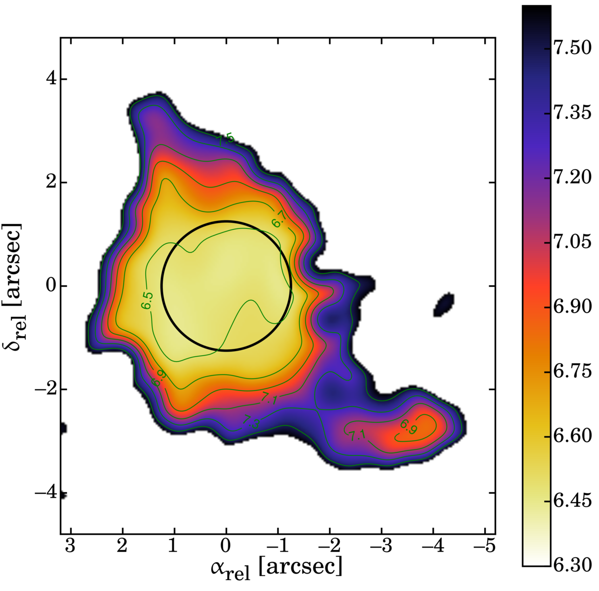
Figure 14: Derived stellar population ages of Tol1247. An age gradient can be identified with a dominating young population in the center and a radial increase in age. The maximum age of the galaxy is $\sim$30 Myr.

5 Summary and Conclusion

We have used the Cosmic Origins Spectrograph (COS) onboard the Hubble Space Telescope (HST) to observe the Ly$\upalpha$ emission line, UV absorption lines (e.g. Si II) and the Lyman continuum of the central region of Tol1247. The data reduction procedure was optimized using a customized range of pulse height amplitude values, filtering for orbital night data and an enhanced background subtraction routine. Furthermore, our modified CALCOS version allows for spectral extractions of individual pixel rows along the x-dispersion. Using these new features, in particular extracting only the central region that firmly encloses the two stellar clusters, we could detect leaking LyC photons in a range of 875–911Å. We have further used the WFC3/UVIS and ACS/SBC onboard the HST to image the galaxy in seven filters (broadband and narrowband). This allowed us to apply LaXs – the Lyman alpha eXtraction software (Hayes et al., 2009) – to perform stellar population synthesis and make predictions of the intrinsic Lyman continuum flux. Using this, the LyC escape fraction was calculated to be 1.5$\pm$0.5%, which is significantly lower than the one recently found by Leitherer et al. (2016). We find that the discrepancy is related to the spectral extraction routine in CALCOS 2.21d, when a superdark frame is provided (see appendix A). The Lyman continuum leakage is further supported by a multitude of other parameters:

• A comparison of the mean Si II and Si IV absorption profiles, suggests that most of the observed gas is ionized, which facilitates LyC escape from density bounded regions.

• With the Si II absorption lines considered, the observations are sensitive to a hydrogen column density of more than $1.1\ \times\ 10^{16}\ cm^{-2}$, which is already optically thick to Ly$\upalpha$ (in agreement with the Ly$\upalpha$ emission profile showing no emission at the systemic velocity), but optically thin to Lyman continuum, giving rise to clear sightlines for Lyman continuum to leak.

• Extractions of the Ly$\upalpha$ emission line along the x-dispersion do not show significant differences in the shape of the P-Cygni profile, suggesting that both stellar clusters that are located in the central region of Tol1247 share a common gas shell.

• From Si II absorption, we derive the covering fraction using the apparent optical depth method and find that the gas clouds are optically thick. However, since residual flux is seen in all velocity bins, the ISM must be sufficiently clumpy. Again a property supporting the direct escape of LyC photons.

• Our H$\upalpha$ images reveal a rich and complex morphology – including arcs – a sign for strong ongoing feedback processes accelerating the ISM and presumably creating channels along the line of sight through which LyC photons escape.

• The radial extinction profile reveals lines of sight of low extinction within the inner $\sim 500\,pc$, in agreement with a clumpy, anisotropic medium facilitating LyC photons to escape directly from the innermost region of the galaxy.

• Tol1247 was imaged with the VLA in 21cm. The line was not detected, but a deep upper limit atomic gas mass of $\lesssim 10^{9}\,M_{\odot}$ was calculated. The gas fraction of Tol1247 is found to be very low with $f_{gas}=\nicefrac{{M_{HI}}}{{M_{*}}}<0.2$.

• A large fraction of the Ly$\upalpha$ emission in Tol1247 arises from a surrounding halo. We find evidence that most of the atomic gas volume present in Tol1247 is traced by the observed Ly$\upalpha$ emission; unlike what is seen in five galaxies from the LARS sample, where the halo seen in Ly$\upalpha$ makes up only a small fraction of what is seen in VLA 21 cm imaging.

• Using a consistent set of SFR calibrations, we find that the SFRs derived from extinction-corrected H$\upalpha$, UV and 1.4 GHz are in good agreement with a roughly continuously ongoing star formation during the last $\sim$30 Myr. This value also agrees well with the age derived from the stellar population synthesis.

Appendix A Ad LyC escape fraction

The LyC escape fraction reported in this paper is significantly lower than the one recently found by Leitherer et al. (2016), hereafter L16. It is important to note that this is not due to the modeled flux density to which the observed flux is compared. In fact, the theoretical flux density reported in our Table 3 is only roughly half of the model flux density reported by L16 ($5.05\ \times\ 10^{-14}erg/s/cm^{2}/\AA$).

We find that the discrepancy is related to the spectral extraction routine in CALCOS 2.21d, when a superdark frame is provided. The routine seems to fail at very low flux levels that may include negative count rates (which likely happens after the superdark is subtracted from a low-signal science frame). We have experimented with spectral extractions along different detector regions such as the nominal background regions, where only noise is expected to be seen. However, even in this case, residual positive flux was reported by CALCOS 2.21d and no negative values were seen in the resulting spectrum. Since this is not an expected behavior, we examined the source code until we could isolate and fix the problem, which we then reported to the CALCOS team.

It is important to note that this is only related to CALCOS 2.21d, which is (to our knowledge) an unofficial release of the pipeline, that will be made available to the community (Leitherer et al., 2016). We are very thankful to C. Leitherer and S. Hernandez who provided us with the code and hope that with this finding we can contribute to the overall success of HST/COS.

References

- Amorín et al. (2016) Amorín R., Muñoz-Tuñón C., Aguerri J. A. L., Planesas P., 2016, A&A, 588, A23
- Anderson & Bedin (2010) Anderson J., Bedin L. R., 2010, PASP, 122, 1035
- Becker et al. (2012) Becker A. C., Homrighausen D., Connolly A. J., Genovese C. R., Owen R., Bickerton S. J., Lupton R. H., 2012, MNRAS, 425, 1341
- Behrens et al. (2014) Behrens C., Dijkstra M., Niemeyer J. C., 2014, A&A, 563, A77
- Bergvall et al. (2013) Bergvall N., Leitet E., Zackrisson E., Marquart T., 2013, A&A, 554, A38
- Bergvall et al. (2016) Bergvall N., Marquart T., Way M. J., Blomqvist A., Holst E., Östlin G., Zackrisson E., 2016, A&A, 587, A72
- Bigiel & Blitz (2012) Bigiel F., Blitz L., 2012, ApJ, 756, 183
- Borthakur et al. (2014) Borthakur S., Heckman T. M., Leitherer C., Overzier R. A., 2014, Science, 346, 216
- Calzetti et al. (2000) Calzetti D., Armus L., Bohlin R. C., Kinney A. L., Koornneef J., Storchi-Bergmann T., 2000, ApJ, 533, 682
- Cano-Díaz et al. (2016) Cano-Díaz M., et al., 2016, ApJ, 821, L26
- Caplan & Deharveng (1986) Caplan J., Deharveng L., 1986, A&A, 155, 297
- Cardelli et al. (1989) Cardelli J. A., Clayton G. C., Mathis J. S., 1989, ApJ, 345, 245
- Condon (1992) Condon J. J., 1992, ARA&A, 30, 575
- Condon et al. (1998) Condon J. J., Cotton W. D., Greisen E. W., Yin Q. F., Perley R. A., Taylor G. B., Broderick J. J., 1998, AJ, 115, 1693
- Cowie et al. (2009) Cowie L. L., Barger A. J., Trouille L., 2009, ApJ, 692, 1476
- Curtis-Lake et al. (2012) Curtis-Lake E., et al., 2012, MNRAS, 422, 1425
- Debes & et al. (2015) Debes J., et al. 2015, COS Instrument Handbook for Cycle 23, 7.0 edn. Baltimore, MD, USA, http://www.stsci.edu/hst/cos
- Deharveng et al. (2001) Deharveng J.-M., Buat V., Le Brun V., Milliard B., Kunth D., Shull J. M., Gry C., 2001, A&A, 375, 805
- Dijkstra (2014) Dijkstra M., 2014, Publ. Astron. Soc. Australia, 31, e040
- Dijkstra et al. (2016) Dijkstra M., Gronke M., Venkatesan A., 2016
- Duval et al. (2015) Duval F., et al., 2015, preprint, (arXiv:1512.00860)
- Fan et al. (2001) Fan X., et al., 2001, AJ, 121, 54
- Fan et al. (2006) Fan X., et al., 2006, AJ, 132, 117
- Feldman et al. (2001) Feldman P. D., Sahnow D. J., Kruk J. W., Murphy E. M., Moos H. W., 2001, J. Geophys. Res., 106, 8119
- Ferrara & Loeb (2013) Ferrara A., Loeb A., 2013, MNRAS, 431, 2826
- Finlator et al. (2016) Finlator K., Oppenheimer B. D., Davé R., Zackrisson E., Thompson R., Huang S., 2016, MNRAS, 459, 2299
- Fox et al. (2014) Fox O. D., et al., 2014, ApJ, 790, 17
- Gehrels (1986) Gehrels N., 1986, ApJ, 303, 336
- Genzel et al. (2010) Genzel R., et al., 2010, MNRAS, 407, 2091
- Genzel et al. (2015) Genzel R., et al., 2015, ApJ, 800, 20
- Gonzaga et al. (2012) Gonzaga 2012, The DrizzlePac Handbook
- Güver & Özel (2009) Güver T., Özel F., 2009, MNRAS, 400, 2050
- Hayes (2015) Hayes M., 2015, Publ. Astron. Soc. Australia, 32, 27
- Hayes et al. (2005) Hayes M., Östlin G., Mas-Hesse J. M., Kunth D., Leitherer C., Petrosian A., 2005, A&A, 438, 71
- Hayes et al. (2009) Hayes M., Östlin G., Mas-Hesse J. M., Kunth D., 2009, AJ, 138, 911
- Hayes et al. (2013) Hayes M., et al., 2013, ApJ, 765, L27
- Hayes et al. (2014) Hayes M., et al., 2014, ApJ, 782, 6
- Hayes et al. (2016) Hayes M., Melinder J., Östlin G., Scarlata C., Lehnert M. D., Mannerström-Jansson G., 2016, preprint, (arXiv:1606.04536)
- Heckman et al. (2001) Heckman T. M., Sembach K. R., Meurer G. R., Leitherer C., Calzetti D., Martin C. L., 2001, ApJ, 558, 56
- Heckman et al. (2011) Heckman T. M., et al., 2011, ApJ, 730, 5
- Henry et al. (2015) Henry A., Scarlata C., Martin C. L., Erb D., 2015, ApJ, 809, 19
- Husemann et al. (2013) Husemann B., et al., 2013, A&A, 549, A87
- Iwata et al. (2009) Iwata I., et al., 2009, ApJ, 692, 1287
- Izotov et al. (2016b) Izotov Y. I., Schaerer D., Thuan T. X., Worseck G., Guseva N. G., Orlitova I., Verhamme A., 2016b, preprint, (arXiv:1605.05160)
- Izotov et al. (2016a) Izotov Y. I., Orlitova I., Schaerer D., Thuan T. X., Verhamme A., Guseva N., Worseck G., 2016a, preprint, (arXiv:1601.03068)
- James et al. (2014) James B. L., Aloisi A., Heckman T., Sohn S. T., Wolfe M. A., 2014, ApJ, 795, 109
- Jaskot & Oey (2013) Jaskot A. E., Oey M. S., 2013, ApJ, 766, 91
- Jones et al. (2013) Jones T. A., Ellis R. S., Schenker M. A., Stark D. P., 2013, ApJ, 779, 52
- Kauffmann et al. (2012) Kauffmann G., et al., 2012, MNRAS, 422, 997
- Kennicutt (1998) Kennicutt Jr. R. C., 1998, ARA&A, 36, 189
- Krist et al. (2011) Krist J. E., Hook R. N., Stoehr F., 2011, in Optical Modeling and Performance Predictions V. p. 81270J, doi:10.1117/12.892762
- Kroupa (2001) Kroupa P., 2001, MNRAS, 322, 231
- Kunth et al. (1998) Kunth D., Mas-Hesse J. M., Terlevich E., Terlevich R., Lequeux J., Fall S. M., 1998, A&A, 334, 11
- Leitet et al. (2011) Leitet E., Bergvall N., Piskunov N., Andersson B.-G., 2011, A&A, 532, A107
- Leitet et al. (2013) Leitet E., Bergvall N., Hayes M., Linné S., Zackrisson E., 2013, A&A, 553, A106
- Leitherer et al. (1995) Leitherer C., Ferguson H. C., Heckman T. M., Lowenthal J. D., 1995, ApJ, 454, L19
- Leitherer et al. (1999) Leitherer C., et al., 1999, ApJS, 123, 3
- Leitherer et al. (2016) Leitherer C., Hernandez S., Lee J. C., Oey M. S., 2016, ApJ, 823, 64
- Lequeux (2005) Lequeux J., 2005, The Interstellar Medium, doi:10.1007/b137959.
- Lilly et al. (2013) Lilly S. J., Carollo C. M., Pipino A., Renzini A., Peng Y., 2013, ApJ, 772, 119
- Madau et al. (2004) Madau P., Rees M. J., Volonteri M., Haardt F., Oh S. P., 2004, ApJ, 604, 484
- Massa & et al. (2013) Massa D., et al. 2013, COS Data Handbook v. 2.0. Baltimore, MD, USA
- Micheva et al. (2015) Micheva G., Iwata I., Inoue A., 2015, IAU General Assembly, 22, 2214081
- Mirabel et al. (2011) Mirabel I. F., Dijkstra M., Laurent P., Loeb A., Pritchard J. R., 2011, A&A, 528, A149
- Mo et al. (2010) Mo H., van den Bosch F. C., White S., 2010, Galaxy Formation and Evolution
- Moos et al. (2000) Moos H. W., et al., 2000, ApJ, 538, L1
- Mostardi et al. (2015) Mostardi R. E., Shapley A. E., Steidel C. C., Trainor R. F., Reddy N. A., Siana B., 2015, ApJ, 810, 107
- Nakajima & Ouchi (2014) Nakajima K., Ouchi M., 2014, MNRAS, 442, 900
- Nestor et al. (2011) Nestor D. B., Shapley A. E., Steidel C. C., Siana B., 2011, ApJ, 736, 18
- Osterbrock & Ferland (2006) Osterbrock D. E., Ferland G. J., 2006, Astrophysics of gaseous nebulae and active galactic nuclei. University Science Books
- Östlin et al. (2014) Östlin G., et al., 2014, ApJ, 797, 11
- Paardekooper et al. (2013) Paardekooper J.-P., Khochfar S., Dalla Vecchia C., 2013, MNRAS, 429, L94
- Pardy et al. (2014) Pardy S. A., et al., 2014, ApJ, 794, 101
- Pardy et al. (2016) Pardy S. A., Cannon J. M., Östlin G., Hayes M., Bergvall N., 2016, AJ, 152, 178
- Pellegrini et al. (2012) Pellegrini E. W., Oey M. S., Winkler P. F., Points S. D., Smith R. C., Jaskot A. E., Zastrow J., 2012, ApJ, 755, 40
- Peng et al. (2010) Peng Y.-j., et al., 2010, ApJ, 721, 193
- Pettini et al. (2002) Pettini M., Rix S. A., Steidel C. C., Adelberger K. L., Hunt M. P., Shapley A. E., 2002, ApJ, 569, 742
- Quider et al. (2009) Quider A. M., Pettini M., Shapley A. E., Steidel C. C., 2009, MNRAS, 398, 1263
- Ranalli et al. (2003) Ranalli P., Comastri A., Setti G., 2003, A&A, 399, 39
- Rivera-Thorsen et al. (2015) Rivera-Thorsen T. E., et al., 2015, ApJ, 805, 14
- Rivera-Thorsen et al. (2017) Rivera-Thorsen T. E., Östlin G., Hayes M., Puschnig J., 2017, ApJ, 837, 29
- Roberts & Haynes (1994) Roberts M. S., Haynes M. P., 1994, ARA&A, 32, 115
- Rodighiero et al. (2011) Rodighiero G., et al., 2011, ApJ, 739, L40