Starvation Dynamics of a Greedy Forager

Abstract

We investigate the dynamics of a greedy forager that moves by random walking in an environment where each site initially contains one unit of food. Upon encountering a food-containing site, the forager eats all the food there and can subsequently hop an additional $\mathcal{S}$ steps without food before starving to death. Upon encountering an empty site, the forager goes hungry and comes one time unit closer to starvation. We investigate the new feature of forager greed; if the forager has a choice between hopping to an empty site or to a food-containing site in its nearest neighborhood, it hops preferentially towards food. If the neighboring sites all contain food or are all empty, the forager hops equiprobably to one of these neighbors. Paradoxically, the lifetime of the forager can depend non-monotonically on greed, and the sense of the non-monotonicity is opposite in one and two dimensions. Even more unexpectedly, the forager lifetime in one dimension is substantially enhanced when the greed is negative; here the forager tends to avoid food in its local neighborhood. We also determine the average amount of food consumed at the instant when the forager starves. We present analytic, heuristic, and numerical results to elucidate these intriguing phenomena.

1 Introduction

A classic approach to account for the phenomenon of foraging is to posit that a forager has perfect knowledge of its environment and adopts an optimum strategy to exploit environmental resources[1, 2, 3, 4, 5, 6, 7]. In this class of models, the motion of the forager is treated in an implicit way, and the rate at which resources are consumed is specified a priori as deterministic and spatially homogeneous [8, 9, 10]. A complementary approach is based on employing a simple or a generalized random walk to find resources. Here, the search efficiency is quantified by the time to reach a specified target. A wide range of models have been investigated, including Lévy walks [11], intermittent walks [12, 13, 14, 15] and persistent random walks [16]. Each of these examples have been shown to minimize this search time under specified conditions. However, these models typically do not consider consumption explicitly.

Recently, an alternative description of foraging dynamics was developed in which the forager has no knowledge of its environment and no intelligence—the starving random walk [17, 18]. In this model, the forager is unaffected by the presence or absence of food and always performs an unbiased random walk. When a forager lands on a food-containing site, all the food at this site is consumed. Upon eating, a forager is fully sated and can subsequently hop $\mathcal{S}$ additional steps without encountering food before it starves. However, if the forager lands on an empty site, the forager goes hungry and comes one time unit closer to starvation. Because there is no replenishment of resources, the local environment of the forager is gradually depleted by consumption. Thus its ultimate fate is to starve to death.

Basic questions for this starving random walk are: What is the dependence of: (a) the total amount of food $\mathcal{N}$ consumed at the instant of starvation and (b) the average lifetime $\mathcal{T}$ of the forager on fundamental parameters—the metabolic capacity $\mathcal{S}$ and the spatial dimension $d$? It was previously found that $\mathcal{N}$ grows as $\sqrt{\mathcal{S}}$ for $d=1$ and as $\mathcal{S}^{\alpha}$ with $\alpha\approx 1.8$ in the ecologically relevant case of $d=2$. Correspondingly, the mean lifetime $\mathcal{T}$ grows linearly with $\mathcal{S}$ for $d=1$, as $\mathcal{S}^{\beta}$ with $\beta\approx 1.9$ in $d=2$, and as $\exp(\mathcal{S}^{\omega})$ for $d\geq 3$, with $\omega\approx 1/2$ in $d=3$, and with $\omega$ a gradually increasing function of $d$ for $d>3$ [17, 18]. A complete understanding of the dependence of the food consumed at starvation and the lifetime on $\mathcal{S}$ and $d$ has not yet been reached.

2 Model and Preview of Results

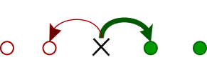
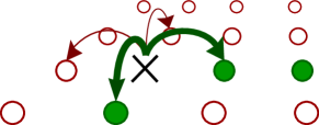
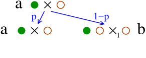
In this work, we investigate a natural extension of the starving random walk to the situation where the forager possesses a minimal level of environmental awareness at the nearest-neighbor level (a preliminary account of these results were given in Ref. [19]). Namely, whenever the nearest neighborhood of a forager contains both empty and full (food-containing) sites, the forager preferentially moves toward one of the full sites (Fig. 1). We will also investigate the opposite situation in which the forager tends to avoid food. We refer to the local propensity to move towards or away from food as “greed”, which is quantified by a greediness parameter $G$, with $-1\leq G\leq 1$. Positive values of $G$ correspond to a forager that moves preferentially towards food in its nearest neighborhood, while for $G<0$, the forager tends to avoid food.

In one dimension, we implement greed as follows: when one neighbor of the forager contains food while the other neighbor is empty, the forager moves towards the food with probability (Fig. 1).

$$p=(1+G)/2\,.$$ (1a)

When the neighboring sites are both empty or both full, then the forager hops equiprobably to the right or to the left. For two and higher dimensions, when there are $$k z-k z$$ neighboring sites that contain food and empty sites (with the lattice coordination number), the forager chooses one of the full sites with probability

$$p={(1+G)}/{\big{[}(z-k)(1-G)+k(1+G)\big{]}}\,.$$ (1b)

(a)  1d

(b)  2d

Figure 1: Motion of a greedy forager ($\times$). Solid and open circles indicate food and empty sites, respectively. Arrow widths indicate relative hopping probabilities.

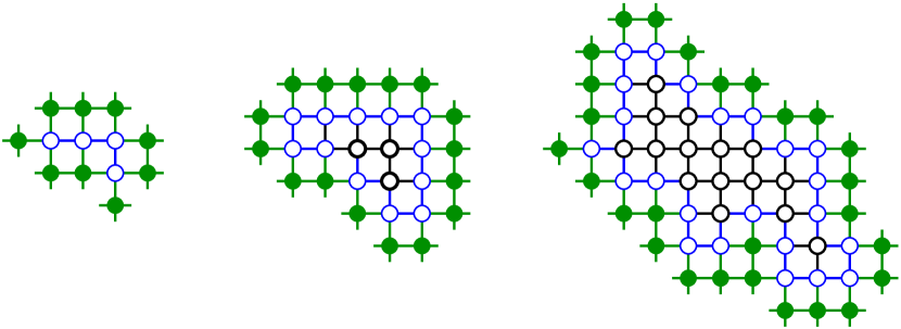
As the walker moves, it creates a depleted region in which food at all sites along its trajectory has been consumed (Fig. 2). We term this region as the “desert”. The desert enlarges each time the forager comes to the perimeter and hops to a food-containing site. Greed modifies the motion of the forager only when it is at the desert perimeter. As the desert grows, the forager typically spends longer time periods wandering within the desert without food. Eventually the forager wanders for $\mathcal{S}$ steps without encountering food and dies of starvation.

Figure 2: (a) Illustration of the desert in one dimension and (b) its growth in two dimensions. Black circles: sites in the desert interior, blue circles: sites on the desert perimeter, green dots: food. At perimeter sites, the forager is biased to move toward food, for $G>0$, or away from food, for $G<0$.

Our implementation of this local greediness represents a particularly simple feedback between the state of the environment and the forager motion. Other classic examples of such feedback include the run and tumble model of chemotaxis [20, 21, 22], in which a bacterium effectively swims up a continuous concentration gradient of nourishment, and infotaxis models [23, 24], in which a forager finds a target by moving up an information gradient. In classic chemotaxsis models, the concentration of nutrients is fixed and unaffected by forager consumption. In contrast, our modeling explicitly incorporates resource depletion; a related type of resource depletion also occurs in autochemotaxis [25, 26, 27].

Our goal is to determine how greed affects the dependence of the average forager lifetime $\mathcal{T}$ on its capacity $\mathcal{S}$. Naively, one might expect that greed is “good” and always increases the forager lifetime. Unexpectedly, we find that greed can be either good or bad, depending on $\mathcal{S}$ and $d$ (Fig. 3). Specifically, the forager lifetime varies non-monotonically with greediness when $\mathcal{S}$ is large, with opposite senses of the non-monotonicity in $d=1$ and $d=2$.

(a) 1d

(b) 2d

Figure 3: Our primary result: Simulation data (discrete points) for the non-monotonic dependence of the scaled average forager lifetime $\mathcal{T}/\mathcal{S}$ on greediness $G=2p-1$ in: (a) one and (b) two dimensions. Error bars are smaller than symbol sizes throughout. Also shown is the analytical prediction for the lifetime; note that the numerical evaluation of (31b) becomes increasingly unstable as $G\to 1$.

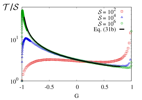
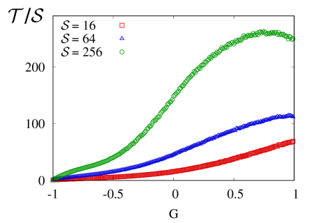
While positive greed seems biologically more relevant, the extension to negative greed, where the forager is food averse, leads to surprising features. By construction, a forager with negative greed preferentially hops away from food when at the boundary of a desert. Naively, one might anticipate that this tendency would decrease the forager lifetime. However, for the one-dimensional “Eden” initial condition, where all sites initially contain one unit of food, the forager lifetime grows dramatically as $G$ decreases toward $-1$ (or equivalently $p$ close to 0) (Fig. 3(a)). This growth in the lifetime stops at a critical value of $G$ that is slightly larger than $-1$; below this point the lifetime again decreases as $G\to-1$, as it must.

We begin, in Sec. 3, by deriving general first-passage properties for a greedy forager in one dimension that moves as a random walk in the desert interior, but is biased either toward or away from food, when the forager is at the desert edge. We then investigate the greedy forager problem in the simpler case of a one-dimensional semi-infinite geometry (Sec. 4), where we derive the exact lifetime. Next, we investigate the forager lifetime for the Eden initial condition in one dimension (Sec. 5). We first present a heuristic argument for the non-monotonic dependence of lifetime on greediness and then develop a rigorous approach for this dependence. We also treat the case of a forager with negative greediness. In Sec. 6 we study greedy forager dynamics in two dimensions.

3 First-Passage Formalism

The dynamics of the greedy forager is governed by the probability that it reaches food in $\mathcal{S}$ steps or less from the last time of its last meal. This quantity is just the time integral of the first-passage probability to reach food up to time $\mathcal{S}$. Because the motion of a greedy forager is different at the boundary of the desert than in the interior, we must extend the first-passage formalism developed in Refs. [17, 18] to account for this boundary perturbation. In this section, we summarize these boundary-perturbed first-passage properties for a greedy forager that will be used in the following sections.

Consider a random walk that is either at $x=1$ or $x=L-1$ in the interval $[0,L]$. Let $f_{L}(t)$ denote the probability that an isotropic random walk first reaches either edge of the interval at time step $t$ with this initial condition. Throughout, all lengths are expressed in dimensionless form in units of the lattice spacing $a$. Now consider a greedy forager at the edge of the interval. It hops toward food with probability $p$ and away from food with probability $1-p$. In the interior of the interval the forager hops symmetrically. We define $F_{L}(t)$ as the probability that this greedy random walk, which starts at either $x=1$ or $x=L-1$, reaches either $x=0$ or $x=L$ at the $t^{\rm th}$ step. These two first-passage probabilities are related by the convolution

$$F_{L}(t)=p\,\delta_{t,1}+(1-p)\sum_{t^{\prime}\leq t-1}f_{L-2}(t^{\prime})\,F_{L}(t-t^{\prime}-1)\,.$$ (2)

The first term accounts for a forager reaching food in a single step. The second term accounts for the forager hopping to the interior of the interval. In the latter case, the walker starts at $x=2$ or $x=L-2$ and hops symmetrically until it again reaches either $x=1$ or $x=L-1$. Thus the relevant first-passage probability is that for an unbiased random walk that starts at $x=2$ or $x=L-2$ in the interval $[1,L-1]$. Once the walker first reaches either $x=1$ or $x=L-1$, the process renews and the subsequent propagation involves $F_{L}$. Since one time unit is used in the first hop to the right, the walker must reach the boundary in the remaining time $t-t^{\prime}-1$ steps.

To solve Eq. (2), we employ the generating functions

$${\widetilde{f}_{L}}(z)=\sum_{t\geq 1}f_{L}(t)\,z^{t}\,,\qquad\qquad{\widetilde{F}_{L}}(z)=\sum_{t\geq 1}F_{L}(t)\,z^{t}\,.$$

to reduce this equation to ${\widetilde{F}_{L}}(z)=pz+(1-p)\,z\,{\widetilde{f}_{L-2}}(z)\,{\widetilde{F}_{L}}(z)$, with solution

$${\widetilde{F}_{L}}(z)=\frac{pz}{1-(1-p)\,z\,{\widetilde{f}_{L-2}}(z)}\,.$$ (3)

We also exploit first-passage ideas to write formal expressions for two basic observables: (a) the average amount of food $\mathcal{N}$ consumed when the forager starves, and (b) the average forager lifetime $\mathcal{T}$. To compute these two quantities, we first define the probability $V_{k}$ that the forager has visited $k$ distinct sites at the instant of starvation; this is the same as the probability that the forager has eaten $k$ times at the instant of starvation. We can express this probability in the form

$$V_{k}=\big{[}1-\mathcal{F}_{k}(\mathcal{S})\big{]}\,\,\prod_{j=1}^{k-1}\mathcal{F}_{j}(\mathcal{S})\,.$$ (4)

Here $\mathcal{F}_{k}(\mathcal{S})$ is the probability that the forager eats before it starves in a desert of $k$ sites, which can be interpreted as the probability that the forager successfully escapes a desert of $k$ sites when it starts one site away from the edge. Thus to create a desert of $k$ sites, the forager must successively escape a desert of $1,2,3,\ldots,k-1$ sites and then fail to escape a desert of $k$ sites. (Note that by definition $\mathcal{F}_{k}(\mathcal{S})=1$.)  In turn, $\mathcal{F}_{k}(\mathcal{S})$ is given by

$$\mathcal{F}_{k}(\mathcal{S})=\sum_{t=0}^{\mathcal{S}}\,F_{k}(t)\,,$$ (5)

where $F_{k}(t)$ is the greedy-forager first-passage probability introduced just above Eq. (2). While we tacitly assume a finite interval length, we will also adapt the formalism above to the case of a semi-infinite interval in the next section.

The average amount of food consumed by the forager at the instant of starvation and the average forager lifetime can now be expressed simply in terms of the distribution of the number of distinct sites visited at starvation (see also [17, 18]):

$$\mathcal{N} =\sum_{k\geq 0}kV_{k}\,,$$ (6a)

$$\mathcal{T} =\sum_{k\geq 0}\,\big{[}\sum_{j=1}^{k-1}\tau_{j}\big{]}\,V_{k}+\mathcal{S}\,,$$ (6b)

where $\tau_{j}=\tau_{j}(\mathcal{S})$ is the average time for a forager to successfully escape a desert of length $j$ by eating a unit of food at the desert edge before starvation is reached. This escape time $\tau_{j}$ may be expressed in terms of the first-passage probability $F_{j}(t)$ of the greedy forager by

$$\tau_{j}=\frac{\sum_{t=0}^{\mathcal{S}}\,t\,F_{j}(t)}{\sum_{t=0}^{\mathcal{S}}\,F_{j}(t)}\,.$$ (7)

In the following sections, we will use these general formulae to compute $\mathcal{N}$ and $\mathcal{T}$ for both the semi-infinite- and finite-desert geometries.

4 One Dimension: Semi-Infinite Desert Geometry

4.1 Heuristic Approach

In this geometry, all sites with $x\leq 0$ initially contain food, all sites with $x\geq 1$ are empty, and the forager begins in a fully sated state at $x=1$. When the forager is extremely greedy, corresponding to $p\to 1$, and also for large $\mathcal{S}$, a typical trajectory consists of segments where the forager moves ballistically into the food-containing region, interspersed by diffusive segments in the desert (Fig. 4). As long as the diffusive trajectory segment lasts less than $\mathcal{S}$ steps, the forager returns to the food/desert interface and another cycle of consumption and subsequent diffusion in the desert begins anew.

Figure 4: Space-time trajectory of a greedy forager with lifetime 271 steps for $p=0.9$ and $\mathcal{S}=100$ (corresponding to $1-p=1/\sqrt{\mathcal{S}}$) in one dimension. Here, the forager quickly carves out a desert whose length precludes reaching the far side at $x=0$; thus the far side is irrelevant.

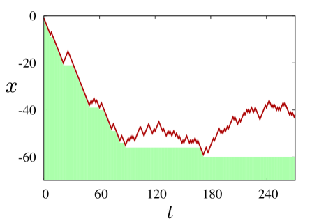
We now exploit this picture of alternating ballistic and diffusive segments to estimate the average forager lifetime. In a typical trajectory, a ballistic segment of $m$ consecutive steps towards food followed by a step away from food occurs with probability $p^{m}(1-p)$. The average time for such a ballistic segment is

$$t_{b}=\sum_{m\geq 1}m\,p^{m}\,(1-p)=\frac{p}{1-p}\,.$$ (8a)

The diffusive segment must return to food within $$\mathcal{S} \mathcal{S} \mathcal{R} D x=1 x=0 \mathcal{S}$$ steps for the forager to survive. Since we are primarily interested in the limit where is large, we may use, without loss of accuracy, continuum expressions to describe the diffusive segments. In this continuum limit, the return probability is the integral of the first-passage probability for a forager with diffusivity that starts at to reach within time  [30]:

$$\mathcal{R}=\int_{0}^{\mathcal{S}}dt\,\,\frac{e^{-1/4Dt}}{\sqrt{4\pi Dt^{3}}}=\mathrm{erfc}(1/\sqrt{4D\mathcal{S}})\,,$$

where erfc$$(\cdot) \langle r\rangle\!=\!\sum_{r\geq 1}r\,\mathcal{R}^{r}(1\!-\!\mathcal{R})\!=\!\mathcal{R}/(1\!-\!\mathcal{R})\!\simeq\!\sqrt{\pi\mathcal{S}/2} \mathcal{S}\to\infty D=\frac{1}{2} \mathcal{S} t_{r}$$ is the complementary error function. Again in the continuum limit, the average number of such successful returns is for , where the asymptotics of the error function gives the final result, and we take the diffusion coefficient to correspond to our discrete random-walk simulations. For a forager that does return within steps, the average return time is

$$t_{r} =\frac{1}{\mathcal{R}}\int_{0}^{\mathcal{S}}dt\,t\,\frac{1}{\sqrt{4\pi Dt^{3}}}\,\,e^{-1/4Dt}\,,$$

$$=\sqrt{\frac{2\mathcal{S}}{\pi}}\,\frac{e^{-1/2\mathcal{S}}}{\text{erfc}(1/\sqrt{2\mathcal{S}})}-1\simeq\sqrt{\frac{2\mathcal{S}}{\pi}}-1\,.$$ (8b)

Here and henceforth the symbol $\simeq$ means asymptotically exact as $\mathcal{S}\to\infty$

Figure 5: (a) Average food consumed $\mathcal{N}$ at starvation for the case $\mathcal{S}=10^{4}$, and (b) average forager lifetime $\mathcal{T}$ versus greediness $G=2p-1$ for $\mathcal{S}=10^{1}$, $10^{2}$, and $10^{3}$. The curve is the prediction (9a), while the circles are the simulation results. In (b), the dashed curves are the continuum predictions (9b), while the solid curves are the exact expression (17).

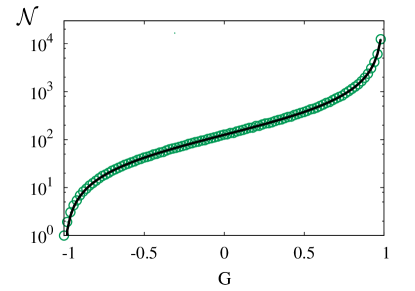
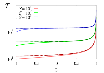
The total trajectory therefore consists of $\langle r\rangle=\sqrt{\pi\mathcal{S}/2}$ elements, each of which are comprised of a ballistic and a diffusive segment. Thus the forager eats $\frac{p}{1-p}$ units of food during each element and the time for each element equals $t_{b}+t_{r}$. There is also the final and fatal diffusive segment of exactly $\mathcal{S}$ steps. Consequently, the food consumed by the forager and its lifetime, which we respectively write as $\mathcal{N}_{\rm SI}$ and $\mathcal{T}_{\rm SI}$ (with the subscript SI denoting the semi-infinite system) respectively, are (Fig. 5)

$$\mathcal{N}_{\rm SI} \simeq\frac{p}{1-p}\,\sqrt{\frac{\pi\mathcal{S}}{2}}\,,$$ (9a)

$$\mathcal{T}_{\rm SI} \simeq\langle r\rangle(t_{b}+t_{r})+\mathcal{S}=\frac{2p-1}{1-p}\,\sqrt{\frac{\pi\mathcal{S}}{2}}+2\mathcal{S}\,.$$ (9b)

For the lifetime, there are two distinct limiting cases:

• Weak greed ($\frac{1}{1\!-\!p}<\sqrt{\mathcal{S}}$): Lifetime linear in $\mathcal{S}$.

• Strong greed ($\frac{1}{1\!-\!p}>\sqrt{\mathcal{S}}$): Lifetime proportional to $\sqrt{\mathcal{S}}$. However, the amplitude of $\sqrt{\mathcal{S}}$ is proportional to $\frac{1}{1-p}$ so that the sublinear term is actually larger than $\mathcal{S}$.

4.2 Asymptotic Solution

We now apply the formalism of Sec. 3 to obtain asymptotic solutions for $\mathcal{N}_{\rm SI}$ and $\mathcal{T}_{\rm SI}$, as well as their underlying distributions. In the semi-infinite geometry, each term in the product in the distribution of visited sites (4) is identical because the desert length is always (semi-)infinite. Thus the length subscripts for all quantities in Sec. 3 can be dropped. From (4), the probability that $k$ units of food have been eaten at the instant of starvation simplifies to $V_{k}=\mathcal{F}^{k}(\mathcal{S})\big{[}1-\mathcal{F}(\mathcal{S})\big{]}$. Thus the average amount of food eaten by the forager at the instant of starvation is

$$\mathcal{N}_{\rm SI}=\sum_{k}kV_{k}=\frac{\mathcal{F}(\mathcal{S})}{1-\mathcal{F}(\mathcal{S})}\,.$$ (10)

To obtain $\mathcal{F}(\mathcal{S})$ we need the underlying first-passage probability (3). We start with the well-known expression for the generating function of the first-passage probability for the isotropic random walk in the semi-infinite geometry, ${\widetilde{f}}(z)=(1-\sqrt{1-z^{2}})/z$ [28], and substitute into Eq. (3) to give

$${\widetilde{F}}(z)=\frac{z}{1+\frac{1-p}{p}\sqrt{1-z^{2}}}\,.$$ (11)

We deduce the long-time behavior of $F(t)$ from the $z\to 1$ behavior of  $\widetilde{F}(z)$, from which we can compute $\mathcal{F}(\mathcal{S})$, and finally the amount of food eaten by the forager when it starves, $\mathcal{N}_{\rm SI}$, and its lifetime $\mathcal{T}_{\rm SI}$. For large $\mathcal{S}$, we obtain, both for $p\gg 1/\sqrt{\mathcal{S}}$ and $p\ll 1/\sqrt{\mathcal{S}}$ (details are given in A),

$$\mathcal{N}_{\rm SI}\simeq\frac{p}{1-p}\sqrt{\frac{\pi\mathcal{S}}{2}}\,,\qquad\mathcal{S}\to\infty\,.$$ (12a)

To compute the average forager lifetime, we need the time $\tau_{k}$ for a forager to escape a desert of length $k$ (Eq. (6b)). In the semi-infinite geometry, all these excursion times are identical, $\tau_{k}=\tau$, so that $\mathcal{T}_{\rm SI}=\tau\mathcal{N}_{\rm SI}+\mathcal{S}$. The derivation of $\tau$ is also given in A and the final result for the lifetime has two different forms depending on whether $p\gg 1/\sqrt{\mathcal{S}}$ or vice versa

$$\mathcal{T}_{\rm SI}\simeq\begin{cases}\displaystyle{2\mathcal{S}+\frac{(p^{2}-4p+2)}{p(1-p)}\sqrt{\frac{\pi\mathcal{S}}{2}}}\,,&\qquad p\gg 1/\sqrt{\mathcal{S}}\,,\\[9.95863pt] \displaystyle{\frac{1}{2}p\mathcal{S}^{2}+p\,\sqrt{\frac{\pi}{18}}\,\mathcal{S}^{3/2}+\mathcal{S}}\,,&\qquad p\ll 1/\sqrt{\mathcal{S}}\,.\end{cases}$$ (12b)

4.3 Exact discrete solution

We now obtain the exact lifetime for any $p$ and $\mathcal{S}$ by enumeration. As a preliminary, first consider small $\mathcal{S}$. In the initial state, labeled $a$ in Fig. 6 the forager is adjacent to the food. For $\mathcal{S}=1$, the system can evolve in only two ways: either the forager moves towards the food, which happens with probability $p$, or the forager moves away. In the former case, the forager eats and the process renews; that is, the system remains in the initial state. In the latter case, the forager necessarily dies after one more step. These evolution steps lead to the state space with two distinct states, $a$ and $b$ (Fig. 6(a)). From this figure, the average lifetime starting from state $a$ satisfies the backward Kolmogorov equation [30]

$$t_{a}=p(1+t_{a})+(1-p)\cdot 2\,,$$

which gives $\mathcal{T}_{1}\!\equiv\!t_{a}(\mathcal{S}\!=\!1)\!=\!(2\!-\!p)/(1\!-\!p)$. This same enumeration can straightforwardly (but more tediously) extended to larger $\mathcal{S}$. After one step, the states of the system for $\mathcal{S}=2$ are identical to those for the case $\mathcal{S}=1$, but the states after two steps are distinct (Fig. 6(b)). The corresponding equations for the lifetime starting from any state are:

$$t_{a} =p\left(1+t_{a}\right)+(1-p)(t_{b}+1)\,,$$

$$t_{b} =\tfrac{1}{2}(t_{c}+1)+\tfrac{1}{2}(t_{d}+1)\,,$$

$$t_{c} =p(t_{a}+1)+(1-p)\,,$$

$$t_{d} =1\,.$$

Figure 6: (a) State space of the semi-infinite system for $\mathcal{S}=1$. Top row: the initial state. Next row: states after the forager hops once. The subscript on the symbol $\times$ denotes the number of time steps that the forager is without food. (b) State space of the semi-infinite system for $\mathcal{S}=2$ and 3.

Solving these equations, the lifetime starting from the initial state $a$ for $\mathcal{S}=2$ is

$$\mathcal{T}_{2}\equiv t_{a}(2)=\frac{2(3-2p)}{(1-p)(2-p)}\,.$$ (13a)

The enumeration for $$\mathcal{S}=3 \mathcal{S}=2 \mathcal{T}_{3}=\mathcal{T}_{2}+1 \mathcal{S}$$ is the same as that for , except that the forager lives exactly one more time step before starving. Thus . Following this same approach, the lifetimes for the next few values of are

$$\mathcal{T}_{4} =\frac{5(5-5p+p^{2})}{(1-p)(8-7p+2p^{2})}\,,\qquad\hskip 48.36958pt\mathcal{T}_{5}=\mathcal{T}_{4}+1,$$ (13b)

$$\mathcal{T}_{6} =\frac{4(28-35p+13p^{2}-2p^{3})}{(1-p)(16-19p+10p^{2}-2p^{3})}\,,\qquad\mathcal{T}_{7}=\mathcal{T}_{6}+1.$$ (13c)

We now systematize this enumeration for arbitrary $\mathcal{S}$. We first split the set of all trajectories into two categories: (a) set P, which contains all paths that return to food before the forager starves and (b) set Q, which contains all paths where the forager starves. With this decomposition, the average lifetime for general $\mathcal{S}$ can be written as

$$\mathcal{T}\,=\,\sum_{\textbf{p}\in\textbf{P}}\mathcal{P}_{\textbf{p}}\left(t_{\textbf{p}}+\mathcal{T}\right)+\sum_{\textbf{q}\in\textbf{Q}}\mathcal{P}_{\textbf{q}}\,\mathcal{S}\,.$$ (14a)

Here $$\mathcal{P}_{\textbf{p}} \mathcal{P}_{\textbf{q}} \textbf{p}\in\textbf{P} \textbf{q}\in\textbf{Q} t_{\textbf{p}} \mathcal{S}$$ and are the probabilities of paths and , and is the time for the forager to return to food via path p. The time for all paths in Q that lead to starvation is simply . Rearranging the above expression gives

$$\mathcal{T}\,=\,\frac{\sum\mathcal{P}_{\textbf{p}}t_{\textbf{p}}+\sum\mathcal{P}_{\textbf{q}}\mathcal{S}}{1-\sum\mathcal{P}_{\textbf{p}}}\,.$$ (14b)

Since the union P $$\cup \sum_{\textbf{p}}\!\mathcal{P}_{\textbf{p}}+\sum_{\textbf{q}}\!\mathcal{P}_{\textbf{q}}=1$$ Q gives all paths, we have . We use this relation to simplify the second term in the numerator to give

$$\mathcal{T}\,=\,\frac{\sum\mathcal{P}_{\textbf{p}}t_{\textbf{p}}}{1-\sum\mathcal{P}_{\textbf{p}}}+\mathcal{S}\,.$$ (14c)

Figure 7: Illustration of paths that reach food in $2n+1=23$ steps with different $k$, the number of times the path is adjacent to food (green strip). The indicated Catalan numbers show the number of possible paths given the constraint of hitting the edge of the desert exactly $k$ times. The total number of solid-dashed, dotted, and solid paths are $\mathcal{C}_{10}$, $\mathcal{C}_{2}\mathcal{C}_{0}\mathcal{C}_{6}$, and $(\mathcal{C}_{0})^{11}$.

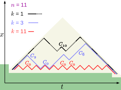
To compute $\sum\mathcal{P}_{\textbf{p}}$, we first note that the probability of a particular path depends only on: (i) its length, which we write as $2n+1$, as a path that starts at $x=1$ can reach food at $x=0$ only in an odd number of steps, and (ii) the number of times $k$ that the path is adjacent to food. The probability of a single path therefore is

$$\mathcal{P}_{\textbf{p}}=\left(\tfrac{1}{2}\right)^{(2n-k)}(1-p)^{k}\,p\,.$$

That is, the forager performs an unbiased random walk for the $(2n-k)$ steps where the forager is not adjacent to food and steps into the desert $k$ times, each with probability $1-p$, when adjacent to food. In the final step, the forager reaches food with probability $p$ (Fig. 7). The sum over all paths that return can be partitioned into sets of paths that are adjacent to the edge of the desert for exactly $k$ steps. The number of paths of this type—of length $2n+1$ with $k$ adjacencies to the desert–is given

$$A(n,k)=\frac{(2n-k-1)!\,k}{(n-k)!\,n!}\,.$$ (15)

The derivation of this result is given in C.

Using this expression for the number of paths, we have

$$\sum\mathcal{P}_{\textbf{p}}=p+p\sum_{n=1}^{\lfloor{\mathcal{S}/2}\rfloor}\sum_{k=1}^{n}A(n,k)(1-p)^{k}\left(\tfrac{1}{2}\right)^{(2n-k)}\,.$$ (16)

The prefactor $p$ before the sum arises from the last segment of the path in which the forager consumes one unit of food. We also write the $n=0$ term separately as it does not conform to the general expression inside the sum. Using Eqs. (14c)–(15), the average lifetime for any $\mathcal{S}$ is given by

$$\mathcal{T}=\frac{p+p\sum_{n=1}^{\lfloor{\mathcal{S}/2}\rfloor}\left[(2n+1)\sum_{k=1}^{n}A(n,k)(1-p)^{k}\left(\frac{1}{2}\right)^{(2n-k)}\right]}{1-p-p\sum_{n=1}^{\lfloor{\mathcal{S}/2}\rfloor}\left[\sum_{k=1}^{n}A(n,k)(1-p)^{k}\left(\frac{1}{2}\right)^{(2n-k)}\right]}+\mathcal{S}\,.$$ (17)

The comparison between this exact lifetime and the continuum expression (12b) is given in Fig. 5(a). The continuum result is an excellent approximation for $p>0.8$ for any $\mathcal{S}$.

5 One Dimension: Finite Desert Geometry

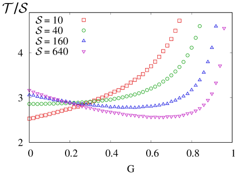
We now turn to the geometry where each site initially contains food—the Eden initial condition—and the forager gradually carves out a finite-length desert. Unexpectedly, the average forager lifetime varies non-monotonically with (positive) greediness when $\mathcal{S}>\mathcal{S}^{*}$, with $\mathcal{S}^{*}\approx 45$ (Fig. 8)—a little greed is bad for a sufficiently “rich” forager, but extreme greed is good.

Figure 8: Simulation data for the average forager lifetime $\mathcal{T}$ versus greediness $G=2p-1$ in one dimension. The survival times have been scaled by $\mathcal{S}$ so that all the data fit onto the same plot.

5.1 Heuristics

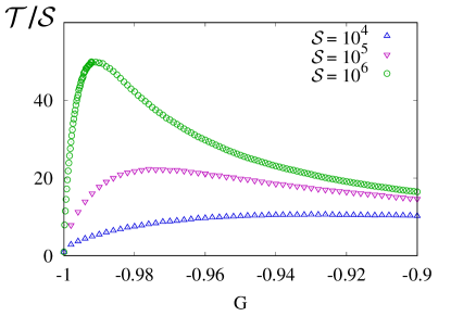
We first present a heuristic argument for both the food consumed at starvation $\mathcal{N}$ and the lifetime $\mathcal{T}$. Our argument predicts both the non-monotonic lifetime for positive greediness and a huge maximum in the lifetime for a negative greediness (Fig. 3(a)). In our approach, starvation proceeds in two stages:

1. The forager first carves a critical-length desert by repeatedly reaching either edge of the desert within $\mathcal{S}$ time steps after food is consumed. The critical length $L_{c}$ is such that a forager of capacity $\mathcal{S}$ typically starves when it attempts to cross a desert of length $L>L_{c}$. We define the time to create a critical-length desert as $\mathcal{T}_{(\text{i})}$ and the food consumed in this phase as $\mathcal{N}_{(\text{i})}$.

2. Once the desert length reaches $L_{c}$, the forager likely starves if it attempts to cross the desert. That is, the far side is unreachable and thus is irrelevant. The time for this second stage, $\mathcal{T}_{(\text{ii})}$ is therefore just the mean lifetime $\mathcal{T}_{\rm SI}$ in a semi-infinite desert. Similarly, the amount of food consumed in this phase is $\mathcal{N}_{\rm SI}$.

To adapt the above argument to a greedy forager, we need the exit probabilities and exit times in a finite interval for the random walk that mimics the motion of the greedy forager—isotropic hopping in the desert interior and hopping towards food with probability $p$ and away from food with probability $1-p$ at the desert edge; these quantities are derived in B. When the forager starts a unit distance from food in a desert of length $L$, the average time to reach food is (Eq. 49)

$$t_{1}=\frac{1-p}{p}\,L+3-\frac{2}{p}\,.$$ (18)

Notice that when $1-p\ll\frac{1}{L}$, the mean time to reach food when starting at $n=1$ approaches 1, while for no greed, $t_{1}=L-1$. By definition

$$\mathcal{N}_{(\text{i})}=L_{c}\,,$$ (19a)

while from (18), the time to reach the critical length $$L_{c}$$ is

$$\mathcal{T}_{(\text{i})}=\frac{1-p}{p}\,\frac{L_{c}(L_{c}+1)}{2}+\Big{(}3-\frac{2}{p}\Big{)}L_{c}\simeq\frac{1-p}{p}\,\frac{L_{c}^{2}}{2}\,.$$ (19b)

For large $\mathcal{S}$ and hence large $L_{c}$, we have

$$\begin{split}\mathcal{N}&=\mathcal{N}_{(\text{i})}+\mathcal{N}_{(\text{ii})}=L_{c}+\mathcal{N}_{\rm SI}\,,\\ \mathcal{T}&=\mathcal{T}_{(\text{i})}+\mathcal{T}_{(\text{ii})}\simeq\frac{1-p}{p}\frac{L_{c}^{2}}{2}+\mathcal{T}_{\rm SI}\,.\end{split}$$ (20)

We now use the crossing time from Eq. (52) for an interval of length $L\gg 1$

$$t_{\times}\approx\frac{2}{3}\,L^{2}+\frac{4}{3}\,\frac{L}{p}\,,$$ (21)

and set $t_{\times}$ equal to $\mathcal{S}$ to give the critical desert length

$$L_{c}\simeq\begin{cases}\sqrt{3\mathcal{S}/2}&\qquad p\gg 1/\sqrt{\mathcal{S}}\,,\\ ~{}3p\mathcal{S}/4&\qquad p\ll 1/\sqrt{\mathcal{S}}\,.\end{cases}$$ (22)

We emphasize that different behaviors arise for $p\gg 1/\sqrt{\mathcal{S}}$ and $p\ll 1/\sqrt{\mathcal{S}}$. Using the expression for $\mathcal{T}_{\rm SI}$ in (12b) together with (20) and (22), we have, for $p\gg 1/\sqrt{\mathcal{S}}$,

$$\mathcal{N} \simeq\sqrt{\frac{3\mathcal{S}}{2}}+\frac{p}{1-p}\,\sqrt{\frac{\pi\mathcal{S}}{2}}\,,$$ (23a)

$$\mathcal{T} \simeq\frac{1-p}{p}\,\frac{3\mathcal{S}}{4}+2\mathcal{S}-\frac{(p^{2}-4p+2)}{p(1-p)}\,\sqrt{\frac{\pi\mathcal{S}}{2}}\,,$$ (23b)

while for $p\ll 1/\sqrt{\mathcal{S}}$

$$\mathcal{N} \simeq\frac{3}{4}\,p\mathcal{S}+\frac{p}{1-p}\,\sqrt{\frac{\pi\mathcal{S}}{2}}\,,$$ (24a)

$$\mathcal{T} \simeq\frac{9}{32}\,p\mathcal{S}^{2}+\mathcal{S}+p\,\sqrt{\frac{\pi}{18}}\,\,\mathcal{S}^{3/2}\,.$$ (24b)

Two important consequences follow from the above expressions for $\mathcal{T}$, as illustrated in Figs. 3 and 8:

• Expanding Eq. (23b) for $p=\frac{1}{2}+\epsilon$ with $\epsilon\to 0$ gives

  $$\mathcal{T}\simeq\frac{11}{4}\mathcal{S}+\Big{(}12\sqrt{\frac{\pi\mathcal{S}}{2}}-10\mathcal{S}\Big{)}\epsilon\,.$$

  Thus the lifetime initially increases with $\epsilon$ for $\mathcal{S}<\mathcal{S}^{*}={18\pi}/{25}$ and initially decreases otherwise. While the numerical value of $\mathcal{S}^{*}$ should not be taken seriously because of the crudeness of our argument, the important point is that $\mathcal{S}$ is a non-monotonic function of greediness for $\mathcal{S}>\mathcal{S}^{*}$ because the lifetime must eventually increase with greediness as $G\to 1$.

• At the crossover, where $p\sim 1/\sqrt{\mathcal{S}}$, Eqs. (23b) and (24b) give the common lifetime $\mathcal{T}\sim\mathcal{S}^{3/2}$. A huge maximum! This maximum arises because the forager eats only when it absolutely must. Because desert is small for $G\approx-1$ (see Eq. (24a)), the strategy of avoiding food until nearly $\mathcal{S}$ steps have elapsed is not that risky.

5.2 First-passage approach

We now determine the amount of food consumed at starvation, $\mathcal{N}$, and the lifetime $\mathcal{T}$ of a greedy forager by extending the approach of Refs. [17, 18] to account for greed. We start with the first-passage probability for pure diffusion in the interval $[0,L]$ and then compute the first-passage probability for greedy forager motion in this same interval. From this, we obtain the probability $\mathcal{F}_{L}(\mathcal{S})$ that the greedy forager can escape a desert of length $L$, as well as the escape time time $\tau_{L}$ for this event. From these two quantities we finally determine $\mathcal{N}$ and $\mathcal{T}$.

The Laplace transform of the first-passage probability for diffusion on $[0,L]$ is [30]

$${\widetilde{f}_{L}}(s)=\frac{\sinh\left(\sqrt{\frac{s}{D}}\right)+\sinh\left(\sqrt{\frac{s}{D}}(L-1)\right)}{\cosh\sqrt{\frac{s}{D}}L} =\cosh\sqrt{\frac{s}{D}}-\tanh\sqrt{\frac{sL^{2}}{4D}}\,\sinh\sqrt{\frac{s}{D}}\,,$$

$$\underset{s\to 0}{\longrightarrow}1-\sqrt{\frac{s}{D}}\tanh\sqrt{\frac{sL^{2}}{4D}}+\cdots\,.$$

Substituting this expression in (3) and converting the generating function to a continuum Laplace transform by replacing $z\to 1-s$, the Laplace transform of the first-passage probability for greedy forager motion for $s\to 0$ and $L\to\infty$ is

$${\widetilde{F}_{L}}(s)=\bigg{(}1+\frac{1-p}{p}\sqrt{\frac{s}{D}}\tanh\sqrt{\frac{sL^{2}}{4D}}\bigg{)}^{-1}.$$ (25)

Note that this expression reproduces the discrete generating function ${\widetilde{F}}(z)$ in Eq. (11) for $L\to\infty$ with $z\to 1-s$ and $D=1/2$. As in the semi-infinite geometry, we must separately examine the limits $p\gg 1/\sqrt{\mathcal{S}}$ and $p\ll 1/\sqrt{\mathcal{S}}$.

The regime $p\gg 1/\sqrt{\mathcal{S}}$:

Since the Laplace variable $s$ corresponds to $1/\mathcal{S}$ for large $\mathcal{S}$, the limit $p\gg 1/\sqrt{\mathcal{S}}$ corresponds to $\sqrt{s}/p\ll 1$. In this case Eq. (25) simplifies to

$${\widetilde{F}_{L}}(s)\simeq 1-\frac{1-p}{p}\sqrt{\frac{s}{D}}\tanh\sqrt{\frac{sL^{2}}{4D}}+\cdots\,.$$ (26)

Since $\mathcal{F}_{L}(\mathcal{S})=\int_{0}^{\mathcal{S}}F_{L}(t)\,dt$ (see Eq. (5)), their Laplace transforms are related by $\widetilde{\mathcal{F}_{L}}(s)={\widetilde{F}_{L}}(s)/s$ [31]. Taking the inverse Laplace transform, the probability that a greedy forager escapes an interval of length $L$ within $\mathcal{S}$ steps is

$$\mathcal{F}_{L}(\mathcal{S})\simeq 1-\frac{1-p}{p}\frac{1}{2\pi i\sqrt{D}}\int_{C}{\rm d}s\,\,e^{s\,\mathcal{S}}\,\frac{1}{\sqrt{s}}\tanh\sqrt{\frac{sL^{2}}{4D}}\,,$$ (27a)

where the vertical segment of the Bromwich contour $$C s_{n}=-D\pi^{2}(2n+1)^{2}/L^{2} n\in{\mathbb{N}}$$ lies to the right of all poles of the integrand. These poles are located at , with , so that

$$\mathcal{F}_{L}(\mathcal{S})\simeq 1-\frac{1-p}{p}\,\frac{4}{L}\sum_{n=0}^{\infty}e^{-D\mathcal{S}\left[\pi(2n+1)\right]^{2}/L^{2}}.$$ (27b)

The above represents the exact Laplace inversion of the asymptotic form for $\widetilde{\mathcal{F}_{L}}(s)$.

To compute the time $\tau_{L}$ for a greedy forager to escape an interval of length $L$, we use the fact that for large $\mathcal{S}$ we can replace the denominator in the definition (7) for $\tau_{L}$, which is the probability for the forager to escape an interval of length $L$ within a time $\mathcal{S}$, by 1. We then use standard Laplace transform manipulations to give, for large $\mathcal{S}$,

$${\widetilde{\tau}_{L}}(s)\simeq-\frac{1}{s}\frac{\partial}{\partial s}{\widetilde{F}_{L}}(s)\,.$$ (28)

Since the $s$-dependent term in Eq. (26) for ${\widetilde{F}_{L}}(s)$ has the prefactor $(1-p)/p$, we have the general relation

$${\widetilde{\tau}_{L}}(s)\simeq\frac{1-p}{p}\,\,{\widetilde{\tau}_{L}}(s;p=\tfrac{1}{2})$$ (29)

between the escape time for the greedy forager and for a pure random-walk forager. Here, the right-hand side is just the escape time for the case $p=1/2$ (random walk). Thus we obtain the fundamental relation between the escape times

$$\tau_{L} \simeq\frac{1\!-\!p}{p}\,\tau_{L}(p=\tfrac{1}{2})=\frac{1\!-\!p}{p}\int_{0}^{\theta}\!\!du\,u\sum_{j=0}^{\infty}\frac{4}{(2j\!+\!1)^{2}}\left\{\!1-e^{-(2j+1)^{2}/u^{2}}\left[1+\left(\!\frac{2j\!+\!1}{u}\!\right)^{2}\right]\!\right\}\,.$$ (30)

For the second line, we copy the expression for $\tau_{L}$ in [17, 18] for the case of no greed, and we express the final result in terms of the natural scaling variable $\theta=L/(\pi\sqrt{D\mathcal{S}})$.

We now use these results for $\mathcal{F}_{L}$ and $\tau_{L}$ to determine $\mathcal{N}$ and $\mathcal{T}$ (see D for details):

$$\mathcal{N}=\mathcal{N}^{*}\,\,\frac{4(1-p)}{p}\int_{0}^{\infty}{\rm d}\theta\exp\left[-\frac{2(1-p)}{p}\sum_{n\geq 0}E_{1}\left(\frac{(2n+1)^{2}}{\theta^{2}}\right)\right]\sum_{n\geq 0}e^{-(2n+1)^{2}/\theta^{2}},$$ (31a)

where $$\mathcal{N}^{*}\equiv\pi\sqrt{D\mathcal{S}} E_{1}(x)=\int_{1}^{\infty}dt\,e^{-xt}/t$$ and is the exponential integral, and

$$\mathcal{T}\simeq\mathcal{S}\,\frac{1\!-\!p}{p}\int_{0}^{\infty}\!\!d\theta\,V_{\theta}\int_{0}^{\theta}\!\!du\,u\sum_{j=0}^{\infty}\frac{4}{(2j\!+\!1)^{2}}\left\{1-e^{-(2j+1)^{2}/u^{2}}\left[1+\left(\frac{2j\!+\!1}{u}\right)^{2}\right]\right\}+\mathcal{S}\,.$$ (31b)

We emphasize that $V_{\theta}$ defined in Eq. (64) depends on $p$, so that the lifetime $\mathcal{T}$ for the greedy forager does not merely equal the lifetime for the non-greedy forager times $(1-p)/p$. The above prediction for $\mathcal{T}$ agrees with our numerical simulations when $\mathcal{S}$ is large (Fig. 3). It is worth mentioning, however that numerical evaluation of (31b), along with (64), is time consuming (multiple nested integrals and sums) and unstable, so that simulation results were more expeditious to obtain in the regime $\mathcal{S}\leq 10^{6}$.

The negative greed regime $p\ll 1/\sqrt{\mathcal{S}}$, $G\approx-1$:

In this regime, the hyperbolic function in Eq. (25) can be replaced by its argument, so that ${\widetilde{F}}_{L}(s)$ simplifies to

$${\widetilde{F}}_{L}(s)\simeq\left(1+\frac{L}{2pD}s\right)^{-1}\,,$$ (32)

while again $\widetilde{\mathcal{F}}_{L}(s)={\widetilde{F}}_{L}(s)/s$. Inverting the above Laplace transform gives

$${\cal F}_{L}({\cal S})\simeq 1-e^{-2pD{\cal S}/L}\,,$$ (33)

while Eq. (28) leads to $\tilde{\tau}_{L}(s)\simeq L/(2pDs)$. Taking the inverse Laplace transform of this quantity immediately gives

$$\tau_{L}(\mathcal{S})\simeq\int_{0}^{\mathcal{S}}tF_{L}(t)\,dt\simeq\frac{L}{2pD}\,.$$ (34)

Figure 9: Simulation data for the dependence of the scaled forager lifetime $\mathcal{T}/\mathcal{S}$ on $G=2p-1$ in the negative greed regime for (a) $G$ in the range $[-1,-0.9]$ and (b) $[-1,-0.998]$ for the case $\mathcal{S}=10^{6}$. Also shown in (b) the full expression from Eq. (76) (solid curve), and the asymptotic result (36b) (dashed curve).

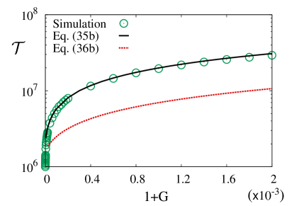
Using the above expression for ${\cal F}_{L}$ and $\tau_{L}$, we find, for ${\cal N}$ and ${\cal T}$ (see D):

$$\mathcal{N} \simeq\sum_{n=1}^{\infty}n\,e^{-{2pD{\cal S}}/{n}}\,\exp\left[-\int_{1}^{n}e^{-{2pD\mathcal{S}}/{k}}\,dk\right]\,,$$ (35a)

$$\mathcal{T} \simeq\frac{1}{2p\cal S}\sum_{n=1}^{\infty}n^{2}\,e^{-{2pD{\cal S}}/{n}}\,\exp\left[-\int_{1}^{n}e^{-{2pD{\cal S}}/{k}}\,dk\right].$$ (35b)

The asymptotic evaluations of these sums and integrals are performed in E, and the final results are

$$\mathcal{N} \simeq\frac{\sqrt{2\pi}}{e}\,\frac{p\,\mathcal{S}}{\ln(p\,\mathcal{S})}\,,$$ (36a)

$$\mathcal{T} \simeq\sqrt{\frac{\pi}{2}}\,\frac{1}{e}\,\frac{p\,\mathcal{S}^{2}}{\big{[}\ln(p\,\mathcal{S})\big{]}^{2}}+\mathcal{S}\,.$$ (36b)

These expressions agree with the naive estimates (24a) and (24b) up to logarithmic corrections. The comparison between the asymptotic prediction for $\mathcal{T}$ in Eq. (36b), the complete form (76), and simulations is shown in Fig. 9(b). The asymptotic approximation becomes increasingly accurate, albeit very slowly, as $\mathcal{S}$ increases. To observe the true asymptotic behavior of greedy forager trajectories by simulations, it would be necessary to treat random walks with $\mathcal{S}\gg 10^{6}$, a range that is practically inaccessible.

6 Greedy Foraging in Two Dimensions

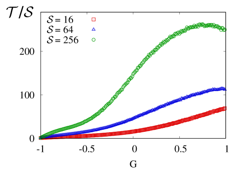
In the dimensions, the desert carved out by a long-lived starving random walker is typically quite ramified [17, 18]. This geometric complexity seems to preclude an analytic solution for the forager lifetime. Instead, we present simulations and heuristic arguments to assess the influence of greed on the forager lifetime. Surprisingly, the role of positive greed in two dimensions is opposite to that in one dimension. For $\mathcal{S}>\mathcal{S}^{*}$, with $\mathcal{S}^{*}\approx 90$, the lifetime again varies non-monotonically with greediness (Fig. 10), but with the opposite sense to the non monotonicity compared to one dimension. An additional perplexing feature, at first sight, is that a perfectly greedy forager has a smaller lifetime than a forager that is not as avaricious.

Figure 10: Average forager lifetime $\mathcal{T}$ versus greediness $G$ in two dimensions. The survival times have been scaled by $\mathcal{S}$ so that they all fit on the same plot.

We can justify this latter feature by appealing to the recurrence of a random walk in two dimensions [28, 29]. Thus there will be many points where the forager trajectory intersects itself, leading to closed loops. Suppose that a perfectly greedy forager is about to form a closed loop on the square lattice, as illustrated in Fig. 11(a). At this point, the forager has only two possible choices for its next step, both of which lead to food being consumed at the next step. One of these choices leads to the outside of the incipient closed loop and the other leads inside. If the latter choice is made, the forager is effectively self trapped by the “moat” that has been created by the previous trajectory.

Figure 11: A random-walk trajectory that leads to trapping of a perfectly greedy forager. (a) Forager ($\times$) at the decision point. (b) Forager hops to the interior region (shaded). (c) Food in the interior is completely consumed, so that the forager ($\times$) may be trapped inside the newly created desert.

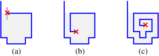
Once inside the moat, a perfectly greedy forager will always consume food in its nearest neighborhood. This consumption is interrupted when all the current neighbors of the forager are empty. When this happens, either the interior is mostly or completely depleted (the latter is shown in Fig. 11(c)). While the former case is more likely, the remaining food will be scarce and isolated. Thus the forager carves out and then becomes trapped inside a (perhaps slightly imperfect) desert. In this circumstance, the forager is likely to starve before it can escape.

Conversely, if the greediness is close to but less than 1, a forager has a non-zero probability to cross the moat whenever it is encountered and thereby reach food on the outside. This mechanism provides a way for the forager to escape the desert and survive longer than if it remained inside. This argument suggests that the forager lifetime must be a decreasing function of $G$ as $G\to 1$, as confirmed by simulations (Fig. 10). Also in stark contrast to one dimension, there is no anomalous peak in the forager lifetime for negative greed, at least for $\mathcal{S}\leq 256$.

7 Discussion

We investigated the dynamics of a greedy forager that either moves preferentially towards food or away from food within its nearest neighborhood. Such a myopic greediness (or anti-greediness) represents a particularly simple mechanism by which the motion of a forager is affected by its environment. In spite of its naiveté, the greedy forager model exhibits rich, unexpected phenomenology that offer theoretical challenges.

As in the starving random walk without greed, a greedy forager depletes its environment by consumption, and one basic issue is to determine the lifetime of the forager as a function of its metabolic capacity $\mathcal{S}$ and its greediness $G$, or equivalently, $p$, the bias that the forager experiences when at the edge of the desert. We determined the forager lifetime exactly in the semi-infinite one-dimensional geometry. Here, the lifetime grows monotonically with greed, as might be expected naively, but the dependence of the lifetime on $\mathcal{S}$ and $p$ is non trivial. For sufficiently strong greed, the forager lifetime scales as $\mathcal{T}\sim\sqrt{\mathcal{S}}/(1-p)$, while for weak greed the lifetime is linear in $\mathcal{S}$.

In the finite desert geometry, we found the unexpected feature that the forager lifetime depends non-monotonically on greediness when the capacity of the forager is sufficiently large. Moreover, the sense of the non-monotonicity is different in one and two dimensions. In one dimension, a little greed is “bad”, while a lot of greed is “good”, where “bad” and “good” mean decreased and increased lifetime, respectively. We gave a heuristic argument based on simple first-passage ideas to understand this non-monotonicity. In two dimensions, the opposite occurs, as a little greed is “good”, while being very greedy is “bad”. We can understand the latter case in a simple way in terms of the self trapping of a forager.

We generalized the first-passage approach of [17, 18] to derive an analytic expression for the average forager lifetime in one dimension that applies in the limit of large $\mathcal{S}$. This approach shows that a small amount of greed is indeed detrimental for the lifetime of the forager in one dimension. Finally, we studied the intriguing case where a forager has negative greed, which means that it avoids food in its local neighborhood. Strikingly, the lifetime of a forager in one dimension exhibits a huge maximum when the greediness $G$ is close to $-1$, or equivalently, $p\to 0$. Using first-passage ideas, we argued that the maximum lifetime occurs at a value of $p$ that scales as $\mathcal{S}^{-1/2}$ and that the lifetime at this maximum scales as $\mathcal{S}^{3/2}$.

There are several open questions about the greedy forager model that deserve further study. First, what is dynamics of a greedy forager in two dimensions? Why is the dependence of lifetime on greed opposite to that of one dimension? Why is there no peak in the lifetime for a forager with very negative greed? What is the nature of the desert geometry for different values of greediness? Second, what is the lifetime of a greedy forager in greater than two dimensions? Simulations are of limited value because the lifetime is extremely long for non-negligible greed and memory and/or computation time constraints become prohibitive. What simulations can say is obvious—in going from no greed to a specified positive value of greediness, the increase in the forager lifetime is much greater in three dimensions than in two. In high dimensions, the mean-field argument given in Refs. [17, 18] still seems to apply; this predicts that the forager lifetime will grow as $e^{\mathcal{S}}$. In the limit of perfect greed, it is always possible to construct analogs of the two-dimensional cul-de-sac of Fig. 11, in which a forager can enter, get trapped, and subsequently starve. Thus the question of whether the forager lifetime depends non-monotonically on greed in greater than two dimensions is still open.

Appendix A Semi-Infinite Geometry

For fixed $p$, the large-$\mathcal{S}$ behavior of the generating function $\widetilde{F}(z)$ in Eq. (11) may be conveniently computed in terms of the generating function for $\mathcal{F}$ in $\mathcal{F}(\mathcal{S})=\sum_{t=0}^{\mathcal{S}}F(t)$. The relation between these two generating functions is [31]

$$\widetilde{\mathcal{F}}(z)=\sum_{\mathcal{S}=0}^{\infty}\mathcal{F}(\mathcal{S})z^{\mathcal{S}}=\frac{{\widetilde{g}}(F)}{1-z}\,.$$ (37)

Differentiating with respect to $z$ gives

$$\sum_{\mathcal{S}=0}^{\infty}\mathcal{S}\mathcal{F}(\mathcal{S})z^{\mathcal{S}} =z\frac{d}{dz}\left(\frac{{\widetilde{F}}(z)}{1-z}\right)$$

$$\mathrel{\mathop{\kern 0.0pt\sim}\limits_{z\to 1}}\frac{1}{(1-z)^{2}}-\frac{1}{\sqrt{2}}\frac{1-p}{p}\frac{1}{(1-z)^{3/2}}-\frac{1}{(1-z)}+\dots$$ (38)

We finally obtain the large-$\mathcal{S}$ behavior of $\mathcal{F}(\mathcal{S})$ by using a discrete Tauberian theorem [29, 32] to give

$$\mathcal{F}(\mathcal{S})=1-\frac{1-p}{p}\sqrt{\frac{2}{\pi\mathcal{S}}}-\frac{1}{\mathcal{S}}+\dots$$ (39a)

For $$p\gg 1/\sqrt{\mathcal{S}} \mathcal{F}(\mathcal{S})$$, we use the above expression for in Eq. (10) to give the result quoted in (12a).

When $p\to 0$ is taken before $\mathcal{S}\to\infty$, we use the following limiting expression of ${\widetilde{F}}(z)$ from Eq. (11),

$$\lim_{p\to 0}\frac{{\widetilde{F}}(z)}{p}=\frac{z}{\sqrt{1-z^{2}}},$$

in (A) to give

$$\lim_{p\to 0}\,\,\frac{\sum_{\mathcal{S}=0}^{\infty}\mathcal{S}\mathcal{F}(\mathcal{S})z^{\mathcal{S}}}{p}\mathrel{\mathop{\kern 0.0pt\sim}\limits_{z\to 1}}\frac{1}{2\sqrt{2}}\,\frac{1}{(1-z)^{5/2}}\,,$$

so that

$$\lim_{p\to 0}\,\,\frac{\mathcal{F}(\mathcal{S})}{p}\mathrel{\mathop{\kern 0.0pt\sim}\limits_{\mathcal{S}\to\infty}}\sqrt{\frac{2\mathcal{S}}{\pi}}\,.$$ (39b)

Substituting the above results for $\mathcal{F}(\mathcal{S})$ in $\mathcal{N}_{\rm SI}=\mathcal{F}(\mathcal{S})/\big{[}1-\mathcal{F}(\mathcal{S})\big{]}$, from Eq. (10), gives

$$\lim_{p\to 0}\,\frac{\mathcal{N}_{\rm SI}}{p}\simeq\sqrt{\frac{\pi\mathcal{S}}{2}}\,,\qquad\mathcal{S}\to\infty\,.$$ (40)

Note that the result for $\mathcal{N}_{\rm SI}$ quoted in Eq. (12a) holds for both $p\gg 1/\sqrt{\mathcal{S}}$ and $p\ll 1/\sqrt{\mathcal{S}}$.

We now determine the escape time $\tau$ for $\mathcal{S}\to\infty$,

$$\tau=\frac{\sum_{t=0}^{\mathcal{S}}tF(t)}{\sum_{t=0}^{\mathcal{S}}F(t)}=\frac{\sum_{t=0}^{\mathcal{S}}tF(t)}{\mathcal{F}(\mathcal{S})}\equiv\frac{\mathcal{F}^{(1)}(\mathcal{S})}{\mathcal{F}(\mathcal{S})}\,.$$ (41)

Following the same reasoning as given above, the generating function for $\mathcal{F}^{(1)}(\mathcal{S})$ is

$$\sum_{\mathcal{S}=0}^{\infty}\mathcal{F}^{(1)}(\mathcal{S})z^{\mathcal{S}}=\frac{z}{1-z}\,{\widetilde{F}}\,^{\prime}(z)\,,$$ (42)

which leads to, as $z\to 1$,

$$\sum_{\mathcal{S}=0}^{\infty}\mathcal{F}^{(1)}(\mathcal{S})z^{\mathcal{S}}=\frac{1}{\sqrt{2}}\frac{1-p}{p}\frac{1}{(1-z)^{3/2}}-\frac{p^{2}-4p+2}{p^{2}}\frac{1}{1-z}+\dots$$ (43)

Using again a Tauberian theorem, the large-$\mathcal{S}$ behavior of $A$ is

$$\mathcal{F}^{(1)}(\mathcal{S})=\frac{2}{\sqrt{\pi}}\frac{1-p}{p}\sqrt{\mathcal{S}}-\frac{(p^{2}-4p+2)}{p^{2}}+\cdots$$

so that

$$\tau=\frac{2}{\sqrt{\pi}}\frac{1-p}{p}\sqrt{\mathcal{S}}-\frac{(p^{2}-4p+2)}{p^{2}}+\cdots$$ (44)

where we have also used Eqs. (39a) and (41). Note that the subleading term in this expansion becomes important when $p\to 1$. Substituting the expression for $\tau$ in $\mathcal{T}_{\rm SI}=\tau\mathcal{N}_{\rm SI}+\mathcal{S}$ gives the final result for the lifetime quoted in Eq. (12b).

If the limit $p\to 0$ is taken before the large-$\mathcal{S}$ limit, the expression Eq. (A) for ${\widetilde{F}}$ has to be used in Eq. (42). This leads to, for $p\to 0$,

$$\frac{\sum_{\mathcal{S}=0}^{\infty}\mathcal{F}^{(1)}(\mathcal{S})z^{\mathcal{S}}}{p}\mathrel{\mathop{\kern 0.0pt\sim}\limits_{z\to 1}}\frac{3\sqrt{2}}{4(1-z)^{5/2}},$$

and thus

$$\frac{\mathcal{F}^{(1)}(\mathcal{S})}{p}\mathrel{\mathop{\kern 0.0pt\sim}\limits_{\mathcal{S}\to\infty}}\sqrt{\frac{2}{9\pi}}\,\mathcal{S}^{3/2}.$$

Using now Eqs. (39b) and (41), we find

$$\tau\!\!\mathrel{\mathop{\kern 0.0pt\sim}\limits_{\mathcal{S}\to\infty}}\frac{1}{3}\,\mathcal{S}\,,$$ (45)

which ultimately leads to Eq. (12b).

Appendix B Escape From An Interval

We determine the first-passage properties of a random walk in a finite interval of length $L$ whose hopping rules are the same as that of a greedy forager. That is, a walk in the interior hops equiprobably to the left and right, while a walk at either $x=1$ or $x=L-1$ hops to the edge of the interval with probability $p$ and into the interior with with probability $1-p$ (Fig. 12). For this walk, we calculate the exit probabilities to each side of the interval, the time to exit either side of the interval, and the conditional exit time to exit by each edge of the interval. We use this information in Sec. 5.1 to argue that the lifetime of a forager with a sufficiently large capacity varies non-monotonically with greediness.

Figure 12: Hopping probabilities for a greedy forager inside a desert of length $L$.

Let $E_{n}$ be the probability that the forager, which starts at site $n$, exits the interval via the left edge. The exit probabilities satisfy the backward equations

$$\begin{split}&E_{1}=p+qE_{2}\,,\\ &E_{n}=\tfrac{1}{2}E_{n-1}+\tfrac{1}{2}E_{n+1}\qquad\qquad 2\leq n\leq L-2\,,\\ &E_{L-1}=qE_{L-2}\,.\end{split}$$ (46)

No boundary conditions are needed, as the distinct equations for $n=1$ and $n=L-1$ fully determine the exit probabilities. As we shall see, $E_{n}=0$ not at $n=L$, but at different value of $n$, and similarly for the point where $E_{n}=1$. This same behavior could be recovered by imposing the radiation boundary condition at $n=0,L$ [29], but this procedure involves subtleties that are tangential to the point of the current derivation.

Since the deviation to random-walk motion occurs only at the boundaries, we attempt a solution that has the random-walk form in the interior of the interval: $E_{n}=A+Bn$. This ansatz automatically solves the interior equations ($2\leq n\leq L-2$), while the boundary equations for $n=1$ and $n=L-1$ give

$$E_{1}=p+qE_{2} ~{}~{}~{}\longrightarrow~{}~{}~{}A+B=p+q(A+2B)\,,$$

$$E_{L-1}=qE_{L-2} ~{}~{}~{}\longrightarrow~{}~{}~{}A+B(L-1)=q\big{(}A+B(L-2)\big{)}\,,$$

from which $A$ and $B$ are

$$A=\frac{p(L-2)+1}{pL+2(1-2p)}\,,\qquad\qquad B=-\frac{p}{pL+2(1-2p)}\,.$$

Thus the probability that a greedy random walk that starts at $x=n$ exits via the left edge of the interval is

$$E_{n}=A+Bn=\frac{L-n+\frac{1}{p}(1-2p)}{L+\frac{2}{p}(1-2p)}\,,$$ (47)

while the exit probability via the right edge is $1-E_{n}$. As might be expected for a perturbation that applies only at the boundary, the overall effect of greed on the exit probability is small: the exit probability changes from $E_{n}=1-\frac{n}{L}$ for $p=\frac{1}{2}$ to $E_{n}=1-\frac{n-1}{L-2}$ for $p=1$. That is, the effective interval length changes from $L$ to $L-2$ as $p$ increases from $\frac{1}{2}$ to 1.

Similarly, let $t_{n}$ be the average time for a greedy random walker to reach either edge of the interval when the walk starts at site $n$. These exit times satisfy the backward equations

$$\begin{split}&t_{1}=p+q(t_{2}+1)\,,\\ &t_{n}=\tfrac{1}{2}t_{n-1}+\tfrac{1}{2}t_{n+1}+1\qquad\qquad 2\leq n\leq L-2\,,\\ &t_{L-1}=p+q(t_{L-2}+1)\,.\end{split}$$ (48)

Again, no boundary conditions are needed, as the equations for $n=1$ and $n=L-1$ are sufficient to solve (LABEL:tn). We attempt a solution for these second-order equations that has the same form as in the case of no greed: $t_{n}=a+bn+cn^{2}$. Substituting this ansatz into (LABEL:tn) immediately gives $c=-1$, while the equations for $t_{1}$ and $t_{L-1}$ lead to the conditions

$$-1+a+b=q(-4+a+2b)+1\,,$$

$$-(L-1)^{2}+b(L-1)+a=q\big{[}-(L-2)^{2}+b(L-2)+a\big{]}+1\,.$$

Solving these equations, the average exit time to either edge of the interval when starting from site $n$ is

$$t_{n}=n(L-n)-\frac{2p-1}{p}(L-2)\,.$$ (49)

This gives a parabolic dependence of $t_{n}$ on $n$ that is shifted slightly downward compared to the case of no greed, as $p$ ranges from $\frac{1}{2}$ to 1. Notice again that $t_{n}=0$ not at $n=0$ and $n=L$, but rather at points between $n=0$ and 1 and between $n=L-1$ and $L$ for $p>\frac{1}{2}$. This overall shift leads to a tiny change in each $t_{n}$, except when the forager starts one site away from the boundary. In this case, the average exit time reduces to the expression given in Eq. (18).

Finally, and for completeness, we determine the conditional exit times, $t^{\pm}_{n}$, defined as the time to reach left edge of the interval when starting from site $n$ (for $t^{-}$) and to the right edge (for $t^{+}$), conditioned on the walker exiting only by the specified edge. We focus on $t^{-}_{n}$, because once $t^{-}_{n}$ is determined, we can obtain $t^{+}_{n}$ via $t^{+}_{n}=t^{-}_{L-n}$. The conditional exit times $t^{-}_{n}$ satisfy

$$\begin{split}&u_{1}=qu_{2}+E_{1}\,,\\ &u_{n}=\tfrac{1}{2}u_{n-1}+\tfrac{1}{2}u_{n+1}+E_{n}\qquad\qquad 2\leq n\leq L-2\,,\\ &u_{L-1}=qu_{L-2}+E_{L-1}\,,\end{split}$$ (50)

where $u_{n}\equiv E_{n}t^{-}_{n}$, with $E_{n}$, the exit probability to the left edge, given by Eq. (47). Because Eqs. (LABEL:un) are second-order with an inhomogeneous term that is linear in $n$, the general solution is a cubic polynomial: $u_{n}=a+bn+cn^{2}+dn^{3}$. Substituting this form into Eq. (LABEL:un) for $2\leq n\leq L-2$, we obtain the conditions $c=-A$ and $d=-B/3$, where $A$ and $B$ are the coefficient of $E_{n}$ in Eq. (47). The remaining two coefficients are determined by solving the equations for $u_{1}$ and $u_{L-1}$ and the final results for the coefficients $a,b,c,d$ in $u_{n}$ are:

$$\begin{split}a&=\frac{2(L-2)(1-2p)\big{[}p^{2}(L-4)(L+\frac{3}{p}(1-p))+3\big{]}}{3p^{3}\big{[}L+\frac{2}{p}(1-2p)\big{]}^{2}}\,,\\ b&=\frac{2p^{2}\big{[}L(L^{2}-6L+6)+8\big{]}+6pL(L-3)+6L-8p}{3p^{2}\big{[}L+\frac{2}{p}(1-2p)\big{]}^{2}}\,,\\ c&=-\frac{L+\frac{1}{p}(1-2p)}{L+\frac{2}{p}(1-2p)}\,,\\ d&=-\frac{1}{3}\,\frac{1}{L+\frac{2}{p}(1-2p)}\,.\end{split}$$ (51)

The conditional exit time to the left edge is then $t_{n}^{-}=u_{n}/E_{n}$, with $u_{n}=a+bn+cn^{2}+dn^{3}$, and $E_{n}$ given by Eq. (47). We are particularly interested in $t^{-}_{L-1}$, the conditional time for a walk that starts at $x=L-1$ to reach $x=0$. From Eqs. (47) and (51), the limiting behavior of this crossing time for large $L$ is given by

$$t^{-}_{L-1}\equiv t_{\times}\simeq\frac{2}{3}\,L^{2}+\frac{4}{3}\,\frac{L}{p}\,,$$ (52)

which is Eq. (21).

Appendix C Catalan Triangle Numbers

We define the number of paths of length $2n$ that are adjacent to food exactly $k$ times as $A(n,k)$. Let $C(n)$ be the ordinary Catalan numbers, which are defined as number of paths that return to the origin in exactly $2n$ steps. These are given by

$$C(n)=\frac{1}{n+1}\binom{2n}{n}$$ (53)

We can write the following convolution form that relates $A(n,k)$ with the Catalan numbers:

$$A(n,k)=\begin{cases}C(n-1)&\qquad k=1\\ \displaystyle{\sum_{j=0}^{n-k}C(j)A(n-j-1,k-1)}&\qquad k\geq 2\,.\end{cases}$$ (54)

This relation can be justified as follows. The number of paths for which the forager returns to the boundary exactly once, namely, at the very end of the trajectory, is given by the ordinary Catalan number. The number of paths where the forager returns $k\geq 2$ times to the boundary can be split into the number of subpaths that return for the first time to the boundary layer at time $2j$, times the number of subpaths that return $k-1$ times to the boundary layer in the remaining $2(n-j-1)$ time steps. This gives the second line in the right-hand side of Eq. (54). We now define the generating functions for $C(n)$ and $A(n,k)$,

$$F(x) =\sum_{n=0}^{\infty}C(n)x^{n}\,,$$ (55a)

$$G(x,y) =\sum_{n=1}^{\infty}\sum_{k=1}^{n}x^{n}y^{k}A(n,k)\,.$$ (55b)

Multiplying the left-hand side of Eq. (54) by $x^{n}y^{k}$ and summing over $n$ and $k$ with the constraint that $k\leq n$, we obtain

$$\sum_{n=1}^{\infty}\sum_{k=1}^{n}x^{n}y^{k}A(n,k) =\sum_{n=1}^{\infty}x^{n}yC(n-1)+\sum_{n=2}^{\infty}\sum_{k=2}^{n}\sum_{j=0}^{n-k}x^{n}y^{k}C(j)A(n-j-1,k-1)\,.$$ (56)

Expressing the above equation in terms of the generating function itself, we obtain $G(x,y)=xyF(x)+xyF(x)G(x,y)$, from which the solution is

$$G(x,y) =\frac{xyF(x)}{1-xyF(x)}\,.$$

Since it is known that $F(x)=2/(1+\sqrt{1-4x})$ [35], we obtain

$$G(x,y)=\frac{2xy}{1+\sqrt{1-4x}-2xy}$$ (57)

To invert Eq. (56), we first expand it in a power series in $y$,

$$G(x,y) =\frac{2xy}{1+\sqrt{1-4x}-2xy}$$

$$=\frac{y}{(1-\sqrt{1-4x})/2x-y}$$

$$=\sum_{k=1}^{\infty}y^{k}\left[\frac{2x}{1-\sqrt{1-4x}}\right]^{k}$$

$$=\sum_{k=1}^{\infty}y^{k}\left[1-\sum_{n=0}^{\infty}C(n)x^{n+1}\right]^{k}\,.$$ (58)

Numerically expanding the above expression in a double power series in $x$ and $y$ using Mathematica, we obtain

$$A(n,k)=\frac{(2n-k-1)!k}{(n-k)!n!}\,.$$ (59)

It is worth noting that the coefficients $A(n,k)$ are related to the Catalan Triangle Numbers [33, 34] $C(n,k)$ by the variable change, $n\to n-1$, $k\to n-k$.

Appendix D Distribution of $\mathcal{N}$ and $\mathcal{T}$

We may generally write the escape probability in a finite interval of length $L$ in the form (see Eq. (27b) and (33))

$$\mathcal{F}_{L}(\mathcal{S})=1-a(L,\mathcal{S})\,,$$ (60)

with $a(L,\mathcal{S})\ll 1$. We determine the behavior of $\prod_{k=2}^{n}\mathcal{F}_{k}(\mathcal{S})$ for large $n$ by considering

$$\ln\prod_{k=2}^{n}\mathcal{F}_{k}(\mathcal{S})=\sum_{k=2}^{n}\ln\big{[}1-a(k)\big{]}\simeq-\sum_{k=2}^{n}a(k)\,.$$ (61)

Thus $V_{n}$ defined in Eq. (4) becomes

$$V_{n}\simeq a(n)\exp\Big{[}-\sum_{k=2}^{n}a(k)\Big{]}\,.$$ (62)

We separately consider the regimes $p\gg 1/\sqrt{\mathcal{S}}$ and $p\ll 1/\sqrt{\mathcal{S}}$. For the former:

$$\sum_{k=2}^{n}a(k) =\frac{4(1-p)}{p}\sum_{k=2}^{n}\,\frac{1}{k}\,\,\sum_{j=0}^{\infty}e^{-D\mathcal{S}[\pi(2j+1)/k]^{2}},$$

$$\simeq\frac{4(1-p)}{p}\int_{0}^{n}\frac{dk}{k}\,\,\sum_{j=0}^{\infty}e^{-D\mathcal{S}[\pi(2j+1)/k]^{2}},$$

$$\simeq\frac{4(1-p)}{p}\int_{0}^{n/\sqrt{\mathcal{S}}}\frac{dk}{k}\,\,\sum_{j=0}^{\infty}e^{-D[\pi(2j+1)/k]^{2}},$$

$$\simeq\frac{2(1-p)}{p}\sum_{n\geq 0}E_{1}\big{(}(2n+1)^{2}/\theta^{2}\big{)}\,,$$ (63)

where $\theta\equiv n/(\pi\sqrt{D\mathcal{S}})$ and $E_{1}(x)\equiv\int_{1}^{\infty}{\rm d}te^{-xt}/t$ is the exponential integral. The distribution of the scaled variable $\theta$ is thus

$$V_{\theta}\simeq\frac{4(1-p)}{p\theta}\sum_{j\geq 0}e^{-(2j+1)^{2}/\theta^{2}}\,\exp\left[-\,\frac{2(1-p)}{p}\sum_{\ell\geq 0}E_{1}\left(\frac{(2\ell+1)^{2}}{\theta^{2}}\right)\right]\,.$$ (64)

The average amount of food consumed by the forager at the instant of starvation is the first moment of this distribution (see (4)) and immediately leads to Eq. (31a).

For $p\ll 1/\sqrt{\mathcal{S}}$, we may write

$$\sum_{k=2}^{n}a(k)\simeq\int_{1}^{n}e^{-{2pD{\cal S}}/k}\,dk,$$ (65)

which leads to

$$V_{n}\simeq e^{-2pD\mathcal{S}/n}\,\exp\left[-\int_{1}^{n}e^{-2pD\mathcal{S}/k}\right]dk\,.$$ (66)

Substituting this result in Eq. (6b) immediately gives Eq. (36b).

Appendix E $\mathcal{N}$ and $\mathcal{T}$ for Extreme Negative Greed in 1d

We now specialize first-passage quantities to the case of extreme negative greed; that is, $G\to-1$ or equivalently, $p\to 0$. Here the enumeration of trajectories to determine the distribution of food consumed at the instant of starvation ($V_{n}$ in Eq. (4)) greatly simplifies because the forager typically moves back to the interior whenever it comes to the edge of the desert. Consider the initial condition $\cdots\bullet\times\bullet\cdots$, which corresponds to the forager being placed at the origin and immediately eating the food at this site. Here $\times$ denotes the forager and $\bullet$ a food-containing site. Now consider the configuration $\bullet\bullet\circ\times\bullet\bullet\cdots$ immediately after the forager has eaten a second time; here $\circ$ denotes an empty site. For the forager to never eat again, it must necessarily bounce back and forth between the two empty sites $\mathcal{S}+1$ times. Because the forager is always at the interface between food and an empty site, each step occurs with probability $1-p$. Thus the probability that it does not eat again before starving, which is the same as the probability that the forager eats exactly twice, is

$$V_{2}=(1-p)^{\mathcal{S}+1}\,,$$

while the probability for the forager to eat more than twice is

$$\mathcal{F}_{2}(\mathcal{S})=1-(1-p)^{\mathcal{S}+1}\,.$$

Generally, $\mathcal{F}_{k}(\mathcal{S})$ was also defined as the probability that the forager eats before it starves in an interval of $k$ empty sites (see (4)). Because the forager has already eaten $k$ times to create this interval, it must eat more than $k$ times to escape this interval.

Suppose now that the forager has eaten a third time. The configuration immediately afterward is $\cdots\bullet\bullet\circ\circ\times\bullet\bullet\cdots$. For the forager to not eat again, it must next hop to the center of the interval, which occurs with probability $(1-p)$, after which the next step necessarily takes the forager back to the edge. To avoid eating, the forager must repeat this pattern of hopping to center and then back to the edge $\mathcal{S}+1$ times. The probability for such a path of $t$ steps is $(1-p)^{t/2}$. Thus starting from $\cdots\bullet\bullet\circ\circ\times\bullet\bullet\cdots$, the forager starves without again eating with probability $(1-p)^{(\mathcal{S}+1)/2}$. Consequently, the probability that the forager eats exactly three times is

$$V_{3}=\mathcal{F}_{2}(\mathcal{S})\,(1-p)^{(\mathcal{S}+1)/2}\,,$$

while the probability that the forager eats more than three times is

$$\mathcal{F}_{2}(\mathcal{S})\mathcal{F}_{3}(\mathcal{S})=\big{[}1-(1-p)^{\mathcal{S}+1}\big{]}\big{[}1-(1-p)^{(\mathcal{S}+1)/2}\big{]}\,.$$

Immediately after eating the fourth time, the configuration is $\cdots\bullet\bullet\circ\circ\circ\times\bullet\bullet\cdots$. To not eat again, the forager must next hop away from the edge, which occurs with probability $(1-p)$. From the resulting state $\cdots\bullet\bullet\circ\circ\times\circ\bullet\bullet\cdots$, the mean time to reach either site at the edge of the desert equals 2 (B). For $t\gg 1$, the forager will be at the edge of the desert $t/3$ times, on average, so that the probability that the forager will starve without eating again is $(1-p)^{(\mathcal{S}+1)/3}$. Thus the probability that the forager eats exactly four times before starving is

$$V_{4}=\mathcal{F}_{2}(\mathcal{S})\mathcal{F}_{3}(\mathcal{S})\,(1-p)^{(\mathcal{S}+1)/3}\,.$$

Continuing this reasoning, the probability that the forager eats more than $n-1$ times before starving is (after changing variables from $\mathcal{S}$ to $z$)

$$\prod_{k=2}^{n-1}\mathcal{F}_{k}(z)=\prod_{k=1}^{n-2}(1-z^{1/k})\,,\qquad\qquad z\equiv(1-p)^{\mathcal{S}+1}\,,$$ (67a)

where we shifted the index in the second product. Thus the probability for the forager to eat exactly $$n$$ times before starving is

$$V_{n}=\prod_{k=2}^{n-1}\mathcal{F}_{k}(z)\,z^{1/(n-1)}\,.$$ (67b)

To compute $\mathcal{N}$ and $\mathcal{T}$ in Eqs. (31a) and (31b), we first investigate the nature of the function $\prod\mathcal{F}_{n}(z)$ in (67a). This function equals 1 for small $n$ and sharply drops to 0 for sufficiently large $n$. Each term in the product equals $(1-z^{1/k})$ and $z$ is, in general, small. Naively, one might think that the point where $\prod\mathcal{F}_{n}$ crosses over from being nearly 1 to decaying would occur when $z^{1/n}=\frac{1}{2}$, or $n=\ln z/\ln\frac{1}{2}$. Numerically, however, $\prod\mathcal{F}_{n}$ is already vanishingly small at this value of $n$ because each term in the product is only slightly different than its immediate predecessor. At the point where a term in the product is close to $\frac{1}{2}$, the product of all previous terms is already close to zero because there are many preceding terms that are also close to $\frac{1}{2}$.

An important consequence of this location of the crossover, is that $z^{1/k}\equiv e^{-a/k}$ is small over the entire range where $\prod\mathcal{F}_{n}$ is non zero. Thus we may simplify $\prod\mathcal{F}_{n}$ by the following standard manipulations:

$$\ln\prod_{k=2}^{n-1}\mathcal{F}_{k} =\ln\Big{[}\prod_{k=1}^{n-2}(1-e^{-a/k})\Big{]}\,,$$

$$=\sum_{k=1}^{n-2}\,\ln(1-e^{-a/k})\,,$$

$$\simeq-\int_{1}^{n}e^{-a/k}\,dk=e^{-a}-n\,e^{-a/n}-a\big{[}E_{1}(a)-E_{1}(a/n)\big{]}\,,$$ (68)

where $E_{1}(\cdot)$ is again the exponential integral. The above form is the explicit representation of the exponential factors in Eqs. (35a) and (35b). We are interested in the regime where $p$ is small, but $p>1/\mathcal{S}$, so that a forager is likely to carve out a desert of an appreciable size. In this case, we have

$$a=-\ln(1-p)^{\mathcal{S}+1}\simeq p\mathcal{S}\,.$$ (69)

Using the representation (E) for $\prod\mathcal{F}_{n}$ as well as $z=e^{-a}$, the amount of food consumed at the instant of starvation is

$$\mathcal{N}=\sum_{n\geq 0}nV_{n} \simeq\int_{0}^{\infty}dn\,n\,e^{-a/n}\,\exp\Big{\{}e^{-a}-n\,e^{-a/n}-a\big{[}E_{1}(a)-E_{1}(a/n)\big{]}\Big{\}}\,,$$

$$=\int_{0}^{\infty}dn\,\exp\Big{\{}\ln n-a/n+e^{-a}-n\,e^{-a/n}-a\big{[}E_{1}(a)-E_{1}(a/n)\big{]}\Big{\}}\,,$$

$$\equiv\int_{0}^{\infty}dn\,\exp\big{[}f(n)\big{]}\,.$$ (70)

The function $f(n)$ in (E) has a single peak whose width vanishes slowly as $a\to\infty$. Thus we evaluate this integral by the Laplace method. Differentiating $f(n)$ in (E) with respect to $n$ and setting the result to zero gives

$$f^{\prime}(n)=\frac{1}{n}+\frac{a}{n^{2}}-e^{-a/n}=0\,.$$ (71)

Numerically, we find that $f$ is maximized at a value $n^{*}$ that grows slightly slower than linearly with $a$. The first natural hypothesis $n^{*}=a/\ln a$, fails to make the terms in (71) balance. Thus we attempt a solution of the form $n^{*}\simeq a(1+\epsilon)/\ln a$, where $\epsilon\ll 1$ for large $a$, and look for a self-consistent solution for $\epsilon$. Substituting in (71), we find that the leading behaviors of the second two terms in this equation are dominant and they balance when

$$n^{*}\simeq\frac{a}{\ln a}\Big{[}1+2\,\frac{\ln\ln a}{\ln a}\Big{]}\,.$$ (72)

To complete the evaluation of the integral (E), we also need the second derivative of $f$ evaluated at $n^{*}$. To leading order, this is

$$f^{\prime\prime}(n^{*})\simeq-\frac{1}{(n^{*})^{2}}-\frac{2a}{(n^{*})^{3}}-\frac{a}{(n^{*})^{2}}\,e^{-a/n^{*}}\simeq-\frac{(\ln a)^{4}}{a^{2}}\,,$$ (73)

where the dominant contribution comes only from the term $(a/n^{2})\,e^{-a/n}$. Finally, we need $f^{*}\equiv f(n^{*})$. Here, we need to keep the first two terms in the asymptotic expansion of $E_{1}$ to obtain, after some straightforward algebra

$$f^{*} =\ln n^{*}-\frac{a}{n^{*}}-\frac{(n^{*})^{2}}{a}\,e^{-a/n^{*}}\simeq\ln\ln a-1\,.$$ (74)

Assembling all these elements gives

$$\mathcal{N} \simeq\int_{0}^{\infty}dn\,\exp\big{[}f(n)\big{]}\sim\sqrt{\frac{2\pi}{|f^{\prime\prime}|}}\,\,e^{f^{*}}\simeq\sqrt{\frac{\pi}{2}}\,\frac{a^{2}}{e}(\ln a)^{-2}\,,$$

$$\sim\frac{\sqrt{2\pi}}{e}\,\frac{p\,\mathcal{S}}{\big{[}\ln(p\,\mathcal{S})\big{]}}\,,$$ (75)

which is Eq. (36a) in the text.

Similarly, the average forager lifetime is

$$\mathcal{T} \simeq\sum_{n\geq 0}\,\frac{n^{2}}{2p}\,V_{n}\simeq\frac{1}{2p}\int_{0}^{\infty}dn\,\exp\big{[}g(n)\big{]}\,,$$ (76)

with $g(n)\equiv f(n)+\ln n$, and $f(n)$ given in (E). Following the same steps as in the evaluation of $\mathcal{N}$, we find the same maximizing value of $n^{*}$, and the same width of the peak, $g^{\prime\prime}(n^{*})=f^{\prime\prime}(n^{*})$, while $g(n^{*})$ now equals $\ln a-1$. Assembling everything gives

$$\mathcal{T} \simeq\frac{1}{2p}\int_{0}^{\infty}dn\,\exp\big{[}f(n)\big{]}+\mathcal{S}\sim\frac{1}{2p}\sqrt{\frac{2\pi}{|f^{\prime\prime}|}}\,\,e^{f^{*}}+\mathcal{S}\simeq\frac{1}{p}\,\sqrt{\frac{\pi}{2}}\,\frac{a^{2}}{e}(\ln a)^{-2}+\mathcal{S}\,,$$

$$\sim\sqrt{\frac{\pi}{2}}\,\frac{1}{e}\,\frac{p\,\mathcal{S}^{2}}{\big{[}\ln(p\,\mathcal{S})\big{]}^{2}}+\mathcal{S}\,.$$ (77)

which is Eq. (36b) in the text.

We should note some caveats about these calculations for $\mathcal{N}$ and $\mathcal{T}$. Normally in applying the Laplace method, the contribution from the peak of the distribution, $e^{f}$, is exponentially larger than the contribution of the width of the maximum, $1/\sqrt{|f^{\prime\prime}|}$. This is not the case here, as the width contribution is almost of the same magnitude as that of the peak (for $\mathcal{T}$) or larger than the peak contribution (for $\mathcal{N}$). In addition, the integrals for $\mathcal{N}$ and $\mathcal{T}$ in Eqs. (E) and (76), respectively, have peaks that are movable. To recast such integrals into a form where the Laplace method can be applied, one normally introduces a rescaled coordinate so as to fix the location of the maximum [36]. If the function in the exponent is algebraic, this rescaling is trivial. However, it does not seem possible to implement such a rescaling for our functions $f(n)$ and $g(n)$. Thus our results (E) and (E) have to be viewed with some suspicion. We checked, however, that the result (E) moves closer to the exact integral (76) as $\mathcal{S}$ increased far beyond the values that we can simulate, but the convergence is extremely slow.

References

- [1] E. L. Charnov, Theor. Popul. Biol. 9, 129 (1976).
- [2] P. Knoppien and J. Reddingius, J. Theor. Biol. 114, 273 (1985).
- [3] D. W. Stephens and J. R. Krebs, Foraging Theory, (Princeton University Press, Princeton, NJ, 1986).
- [4] W. J. O’Brien, H. I. Browman, and B. I. Evans, Am. Sci. 78, 152 (1990).
- [5] J. W. Bell, Searching Behaviour, the Behavioural Ecology of Finding Resources, Animal Behaviour Series (Chapman and Hall, London, 1991).
- [6] J. P. Anderson, D. W. Stephens, and S. R. Dunbar, Behav. Ecol. 8, 307 (1997).
- [7] L. D. Kramer and R. L. McLaughlin, Am. Zool. 41, 137 (2001).
- [8] A. Oaten, Theor. Popul. Biol. 12, 263 (1977).
- [9] Y. Iwasa, M. Higashi, and N. Yamamura, Amer. Nat.117, 710 (1981).
- [10] R. F. Green, Amer. Nat. 123, 30 (1984).
- [11] G. Viswanathan, S. V. Buldyrev, S. Havlin, M. Da Luz, E. Raposo, and H. E. Stanley, Nature 401, 911 (1999).
- [12] O. Bénichou, M. Coppey, M. Moreau, P.-H. Suet, and R. Voituriez, Phys. Rev. Lett. 94, 198101 (2005).
- [13] G. Oshanin, H. Wio, K. Lindenberg, and S. Burlatsky, J. Phys. Condens. Matter 19, 065142 (2007).
- [14] M. A. Lomholt, K. Tal, R. Metzler, and K. Joseph, Proc. Natl. Acad. Sci. (USA) 105, 11055 (2008).
- [15] P. C. Bressloff and J. M. Newby, Phys. Rev. E 83, 061139 (2011).
- [16] V. Tejedor, R. Voituriez, and O. Bénichou, Phys. Rev. Lett. 108, 088103 (2012).
- [17] O. Bénichou and S. Redner, Phys. Rev. Lett. 113, 238101 (2014).
- [18] M. Chupeau, O. Bénichou, and S. Redner, J. Phys. A: Math. & Theor. 49, 394003 (2016).
- [19] U. Bhat, S. Redner, and O. Bénichou, Phys. Rev. E 96, 062119 (2017).
- [20] H. C. Berg and D. A. Brown, Nature 239, 500 (1972).
- [21] H. C. Berg and E. M. Purcell, Biophys. J. 20, 193 (1977).
- [22] P. N. Devreotes and S. H. Zigmond, Annu. Rev. Cell Biol. 4, 649 (1988).
- [23] E. Balkovsky and B. I. Shraiman, Proc. Natl. Acad. Sci. (USA) 99, 12589 (2002).
- [24] M. Vergassola, E. Villermaux, and B. I. Shraiman, Nature 445, 406 (2007).
- [25] R. Grima, Phys. Rev. Lett. 95, 128103 (2005).
- [26] L. Tweedy, D. A. Knecht, G. M. Mackay, and R. H. Insall, PLoS Biol. 14, e1002404 (2016).
- [27] C. Jin, C. Kruger, and C. C. Maass, Proc. Natl. Acad. Sci. (USA) 114, 5099 (2017).
- [28] W. Feller, Introduction to Probability Theory and its Applications, ed., (J. Wiley & Sons, New York, 1968)
- [29] G. H. Weiss, Aspects and Application of the Random Walk, (North-Holland, Amsterdam, 1994).
- [30] S. Redner, A Guide to First-Passage Processes, (Cambridge University Press, Cambridge, UK, 2001).
- [31] G. B. Arfken, H. J. Weber, and F. E. Harris, Mathematical Methods for Physicists: A Comprehensive Guide, ed., (Academic Press, Waltham, MA, 2013).
- [32] G. H. Hardy, Divergent Series, (Oxford University Press, Oxford, UK, 1949).
- [33] D. F. Bailey, Math. Mag. 69, 128 (1996).
- [34] K.-H. Lee and S.-J. Oh, arXiv.org: 1601.06685.
- [35] R. P. Stanley, Enumerative Combinatorics, Vol. 2, (Cambridge University Press, Cambridge, UK, 1999).
- [36] C. M. Bender and S. O. Orszag, Advanced Mathematical Methods for Scientists and Engineers, (McGraw-Hill, New York, 1978).