Stability and instability of the sub-extremal Reissner-Nordström black hole interior for the Einstein-Maxwell-Klein-Gordon equations in spherical symmetry

Abstract

We show non-linear stability and instability results in spherical symmetry for the interior of a charged black hole -approaching a sub-extremal Reissner-Nordström background fast enough- in presence of a massive and charged scalar field, motivated by the strong cosmic censorship conjecture in that setting :

1. Stability : We prove that spherically symmetric characteristic initial data to the Einstein-Maxwell-Klein-Gordon equations approaching a Reissner-Nordström background with a sufficiently decaying polynomial decay rate on the event horizon gives rise to a space-time possessing a Cauchy horizon in a neighbourhood of time-like infinity. Moreover if the decay is even stronger, we prove that the space-time metric admits a continuous extension to the Cauchy horizon. This generalizes the celebrated stability result of Dafermos for Einstein-Maxwell-real-scalar-field in spherical symmetry.

2. Instability : We prove that for the class of space-times considered in the stability part, whose scalar field in addition obeys a polynomial averaged-$L^{2}$ (consistent) lower bound on the event horizon, the scalar field obeys an integrated lower bound transversally to the Cauchy horizon. As a consequence we prove that the non-degenerate energy is infinite on any null surface crossing the Cauchy horizon and the curvature of a geodesic vector field blows up at the Cauchy horizon near time-like infinity. This generalizes an instability result due to Luk and Oh for Einstein-Maxwell-real-scalar-field in spherical symmetry.

This instability of the black hole interior can also be viewed as a step towards the resolution of the $C^{2}$ strong cosmic censorship conjecture for one-ended asymptotically flat initial data.

Contents

1. 1 Introduction
   1. 1.1 Context of the problem and earlier works
   2. 1.2 A first version of the main results
   3. 1.3 Ideas of proof and methods employed
   4. 1.4 Outline of the paper
   5. 1.5 Acknowledgements
2. 2 Geometric framework and equations
   1. 2.1 The equations in geometric form
   2. 2.2 Metric in null coordinates, mass, charge and main notations
   3. 2.3 The Reissner-Nordström solution
   4. 2.4 The Einstein-Maxwell-Klein-Gordon equations in null coordinates
3. 3 Precise statement of the main results
   1. 3.1 Preliminaries on characteristic initial value problem and coordinate choice
   2. 3.2 The stability theorem
   3. 3.3 The instability theorem
4. 4 Proof of the stability Theorem 3.2
   1. 4.1 Strategy of the proof
   2. 4.2 A calculus lemma
   3. 4.3 The event horizon
   4. 4.4 The red-shift region
   5. 4.5 The no-shift region
   6. 4.6 The early blue-shift transition region
   7. 4.7 The late blue-shift region
5. 5 Proof of the instability Theorem 3.3
   1. 5.1 Recalling the stability estimates
   2. 5.2 Reduction to the proof of (3.5)
   3. 5.3 Strategy to prove (3.5)
   4. 5.4 Up to the blue-shift region : the past of $\gamma^{\prime}$
   5. 5.5 Towards the Cauchy horizon : the future of $\gamma^{\prime}$
6. A A localisation of the apparent horizon $\mathcal{A}$
7. B Proof of Proposition 4.7 of section 4.5.1
8. C Proof of Lemma 4.3 of section 4.3.2

1 Introduction

In this paper, we study the stability and instability of the Reissner-Nordström Cauchy horizon for the Einstein-Maxwell-Klein-Gordon equations in spherical symmetry :

$$Ric_{\mu\nu}(g)-\frac{1}{2}R(g)g_{\mu\nu}=\mathbb{T}^{EM}_{\mu\nu}+\mathbb{T}^{KG}_{\mu\nu},$$ (1.1)

$$\mathbb{T}^{EM}_{\mu\nu}=2\left(g^{\alpha\beta}F_{\alpha\nu}F_{\beta\mu}-\frac{1}{4}F^{\alpha\beta}F_{\alpha\beta}g_{\mu\nu}\right),$$ (1.2)

$$\mathbb{T}^{KG}_{\mu\nu}=2\left(\Re(D_{\mu}\phi\overline{D_{\nu}\phi})-\frac{1}{2}(g^{\alpha\beta}D_{\alpha}\phi\overline{D_{\beta}\phi}+m^{2}|\phi|^{2})g_{\mu\nu}\right),$$ (1.3)

$$\nabla^{\mu}F_{\mu\nu}=\frac{q_{0}}{2}i(\phi\overline{D_{\nu}\phi}-\overline{\phi}D_{\nu}\phi),\;F=dA,$$ (1.4)

$$g^{\mu\nu}D_{\mu}D_{\nu}\phi=m^{2}\phi,$$ (1.5)

where the constants $m^{2}$ and $q_{0}$ are respectively called the mass and the charge of the scalar field $\phi$.

This problem is motivated by Penrose’s strong cosmic censorship conjecture (c.f section 1.1.1.) which claims that general relativity is a deterministic theory. The general strategy to address this question is to exhibit a singularity at the boundary of the maximal domain of predictability, which can be done with instability estimates.

We prove that assuming an upper and lower bound on the scalar field $\phi$ on the event horizon of the black hole, the Cauchy horizon exhibits both stability and instability features, namely :

1. Stability : the perturbed black hole still admits a Cauchy horizon -near time-like infinity- like the original unperturbed Reissner-Nordström black hole, and in some cases we can even extend the metric continuously beyond this Cauchy horizon.

2. Instability : the curvature along the Cauchy horizon blows up, which represents an obstruction to a $C^{2}$ extension, at least near time-like infinity. As a by-product, we see that the metric is not $C^{1}$ for the constructed continuous extension.

Similar results are known in the special case $m^{2}=q_{0}=0$ see [14] and [26]. However, in our case the expected decay of the scalar field on the event horizon is much slower, which makes the stability part more difficult. The previous instability result depends strongly on the special structure of the equation in the absence of mass and charge of the scalar field . When $q_{0}\neq 0$ but $m^{2}=0$, a previous work of Kommemi [23] shows a stability result but his assumed decay on the event horizon is only expected to hold for a sub-range of the charge $q_{0}$ that depends on the black hole parameters. In [26], the key argument for the instability is to use an almost conservation law that exists only in the absence of mass and charge. This is the underlying reason why [23] does not contain any instability result.

This work can also be viewed as a first step towards the understanding of the spherically symmetric charged black holes with one-ended initial data. This is because when the scalar field is uncharged, the total charge of the space-time arises completely from the topology. On the contrary, the model that we consider allows for a dynamical total charge which makes $\mathbb{R}^{3}$ type initial data possible.

The introduction is outlined as follows : in section 1.1 we present the strong cosmic censorship conjecture and mention earlier works, then in section 1.2 we explain the reasons to study a charged and massive scalar field and give the results of the present paper. We then sketch the methods of proof in the last section 1.3. Finally in section 1.4 we outline the rest of the paper.

1.1 Context of the problem and earlier works

1.1.1 Strong cosmic censorship conjecture

The study of self-gravitating isolated bodies relies crucially on the vacuum Einstein equation :

$$Ric_{\mu\nu}(g)-\frac{1}{2}R(g)g_{\mu\nu}=0.$$ (1.6)

The simplest non-trivial solution, discovered by Schwarzschild is a spherically symmetric family of black holes, indexed by their mass. These black holes exhibit a very strong singularity, as observers that fall into them experience infinite tidal deformations.

A more sophisticated family of solutions indexed by mass and angular momentum and which describes rotating black holes has been discovered by Kerr in 1963. Unfortunately, Kerr’s black holes have the very undesirable feature that they break determinism : the maximal globally hyperbolic development of their initial data is future extendible as a smooth solution to the Einstein equation (1.6) in many non-unique ways. In some sense, it represents a failure of global uniqueness of solutions.

One way to restore determinism which has been suggested by numerous heuristic and numerical works is that Kerr black holes feature of non-unique extendibility is non-generic, in other words whenever their initial data is slightly perturbed then the maximal globally hyperbolic development is actually future inextendible as a suitably regular Lorentzian manifold.

The nature of this singularity was controversial though : it was widely debated in the physics community whether perturbations of Kerr black holes exhibit a Schwarzschild black hole like singularity and observers experience infinite tidal deformations when they get close to it. One convenient way -although not exactly equivalent- to formulate this question geometrically is to study $C^{0}$ inextendibility.

The inextendibility question has been formulated by Penrose in the following conjecture :

Conjecture 1.1 ( Strong Cosmic Censorship, Penrose).

Maximal globally hyperbolic developments of asymptotically flat initial data are generically future inextendible as a suitably regular Lorentzian manifold .

In the case of $C^{0}$ inextendibility, suitably regular is to be understood as continuous.

Remark 1.

Without the word “generically”, the conjecture is false since Kerr black holes would provide counter examples, in the sense that they have a Cauchy horizon over which the metric can be smoothly extended in a non-unique way. Strong cosmic censorship claims that these counter examples are non-generic.

Due to the complexity of the Kerr geometry, early works on this problem studied instead Reissner-Nordström charged black holes. Although there are not solutions to the vacuum Einstein equation (1.6), they solve the Einstein-Maxwell equations :

$$Ric_{\mu\nu}(g)-\frac{1}{2}R(g)g_{\mu\nu}=\mathbb{T}^{EM}_{\mu\nu},$$ (1.7)

$$\mathbb{T}^{EM}_{\mu\nu}=2\left(g^{\alpha\beta}F_{\alpha\nu}F_{\beta\mu}-\frac{1}{4}F^{\alpha\beta}F_{\alpha\beta}g_{\mu\nu}\right),$$ (1.8)

$$\nabla^{\mu}F_{\mu\nu}=0,\;dF=0.$$ (1.9)

Reissner-Nordström black holes have the same global geometry as Kerr’s but have the simplifying feature that they are spherically symmetric.

In their pioneering numerical work [36], Penrose and Simpson studied linear test fields on Reissner-Nordström black holes and discovered an instability of the Cauchy horizon.

Later Hiscock in [22], Poisson and Israel in [30], [32] exhibited - in a spherically symmetric but non-linear setting- a so-called weak null singularity with an expected curvature blow-up i.e a $C^{2}$ explosion of the metric, but finite tidal deformations allowing for a $C^{0}$ extension.

They studied the Einstein-null-dust equations which model non self-interacting matter transported on null geodesics :

$$Ric_{\mu\nu}(g)-\frac{1}{2}R(g)g_{\mu\nu}=\mathbb{T}_{\mu\nu},$$ (1.10)

$$\mathbb{T}_{\mu\nu}=f^{2}\partial_{\mu}u\partial_{\nu}u+h^{2}\partial_{\mu}v\partial_{\nu}v,$$ (1.11)

$$g^{\mu\nu}\partial_{\mu}u\partial_{\nu}u=0$$ (1.12)

$$g^{\mu\nu}\partial_{\mu}v\partial_{\nu}v=0$$ (1.13)

$$g^{\mu\nu}\partial_{\mu}u\partial_{\nu}f+(\Box_{g}u)f=0$$ (1.14)

$$g^{\mu\nu}\partial_{\mu}v\partial_{\nu}h+(\Box_{g}v)h=0$$ (1.15)

In his seminal work [13], [14], Dafermos studied mathematically the non-linear stability of Reissner-Nordström black holes in spherical symmetry for the Einstein-Maxwell-Scalar-Field equations :

$$Ric_{\mu\nu}(g)-\frac{1}{2}R(g)g_{\mu\nu}=\mathbb{T}^{EM}_{\mu\nu}+\mathbb{T}^{SF}_{\mu\nu},$$ (1.16)

$$\mathbb{T}^{EM}_{\mu\nu}=2\left(g^{\alpha\beta}F_{\alpha\nu}F_{\beta\mu}-\frac{1}{4}F^{\alpha\beta}F_{\alpha\beta}g_{\mu\nu}\right),$$ (1.17)

$$\mathbb{T}^{SF}_{\mu\nu}=2\left(\partial_{\mu}\phi\partial_{\nu}\phi-\frac{1}{2}(g^{\alpha\beta}\partial_{\alpha}\phi\partial_{\beta}\phi)g_{\mu\nu}\right),$$ (1.18)

$$\nabla^{\mu}F_{\mu\nu}=0,\;dF=0,$$ (1.19)

$$g^{\mu\nu}\nabla_{\mu}\nabla_{\nu}\phi=0.$$ (1.20)

Dafermos studied the interior of the black hole and proved conditionally the existence of a Cauchy horizon near time-like infinity with a $C^{0}$ extension for the metric, but $C^{1}$ inextendibility of the $C^{0}$ extension which manifests itself by the blow-up of the (Hawking) mass, which partially confirmed the insights from the work of Poisson-Israel.

Later Dafermos and Rodnianski in [16] proved a stability result on the black hole exterior (c.f section 1.23) which combined with [14] ruled out the $C^{0}$ inextendibility scenario :

Theorem 1.2 (Dafermos [14], Dafermos-Rodnianski [16] ).

For the Einstein-Maxwell-Scalar-Field equations (1.16),(1.17),(1.18), (1.19), (1.20) in spherical symmetry, the ${C^{0}}$ strong cosmic censorship is false.

The question was finally settled in the work of Luk and Oh [26], [27] : they confirmed the weak null singularity scenario, due to a curvature instability :

Theorem 1.3 (Luk-Oh [26], [27] ).

For the Einstein-Maxwell-Scalar-Field equations (1.16),(1.17),(1.18),(1.19),(1.20) in spherical symmetry, the $C^{2}$ strong cosmic censorship conjecture is true.

1.1.2 Earlier works relating to singularities at the Cauchy horizon

As sketched in the previous section, singularities are tightly related to extendibility question. For the stability of the Cauchy horizon, recent progress have been made in different directions c.f [19], [21] for the linear stability, [28], [29] for the linear instability and [23] for the non-linear problem.

In this section, we review in more details stability and instability results in the black hole interior established in previous works leading to the proof of the $C^{2}$ strong cosmic censorship conjecture. These results should be compared to the main theorems of this paper, stated in section 3.

In [14], Dafermos proves a ${C}^{0}$ stability and a ${C}^{1}$ instability result of the Reissner-Nordstrom solution for an uncharged massless scalar field perturbation suitably decaying along the event horizon.

The instability essentially relies on a blow-up of the modified mass $\varpi$ over the Cauchy horizon,as a consequence of a lower bound on the scalar field. Hence the metric is not ${C}^{1}$ extendible in spherical symmetry.

Theorem 1.4 ($\mathcal{C}^{0}$ stability, ${C}^{1}$ instability, Dafermos [14]).

Let $(M,g,\phi,F)$ be a solution of the Einstein-Maxwell-Scalar-Field equations in spherical symmetry such that for some $s>\frac{1}{2}$, we have on the event horizon parametrized by the coordinate $v$ as defined by gauge (3.1) of Theorem 3.2 :

$$|\phi|_{|\mathcal{H}^{+}}(0,v)+|\partial_{v}\phi|_{|\mathcal{H}^{+}}(0,v)\lesssim v^{-s},$$

then :

1. Existence of a Cauchy horizon : in a neighbourhood of time-like infinity, the space-time has the Penrose diagram of Figure 1.

2. Continuous extension : if moreover $s>1$ then the metric g and the scalar field $\phi$ extend as continuous functions along the Cauchy horizon $\mathcal{CH}^{+}$. Moreover, the extended metric can be chosen to be spherically symmetric.

3. Mass inflation and $C^{1}$ inextendibility : coming back to general case $s>\frac{1}{2}$, if we assume the following point-wise lower bound on the scalar field for some $\epsilon>0$ :

   $$v^{-3s+\epsilon}\lesssim|\partial_{v}\phi|_{|\mathcal{H}^{+}}\lesssim v^{-s},$$

   then , the modified mass blows up as one approaches the Cauchy horizon : $\varpi(u,v)\rightarrow_{v\rightarrow+\infty}+\infty$ hence it is impossible to extend the metric g to a spherically symmetric $C^{1}$ metric across the Cauchy horizon $\mathcal{CH}^{+}$. In particular the constructed $C^{0}$ extension is not $C^{1}$.

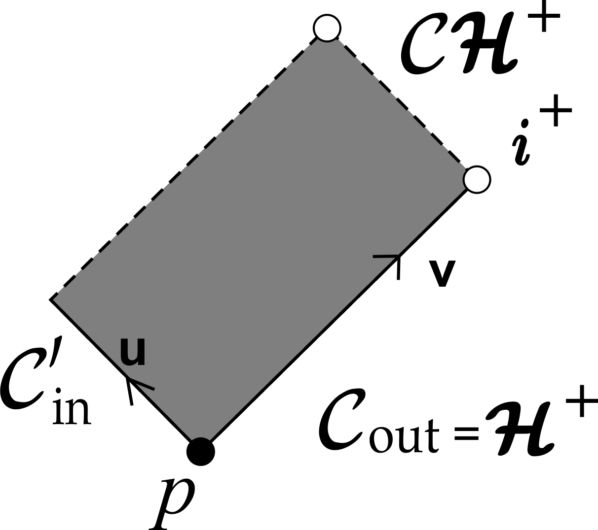
Figure 1: Penrose diagram for the characteristic initial value problem appearing in [14] .

In contrast, the $C^{2}$ strong cosmic censorship conjecture paper dealing with the black hole interior [26] relies on an averaged polynomial decay, as opposed to point-wise and proves a curvature instability :

Theorem 1.5 ( ${C}^{2}$ instability Luk-Oh [26]).

Under the same hypothesis as Theorem 1.4, we also assume that $s>2$ and the following lower bound holds for some $2s-1\leq p<4s-2$ and some $C>0$ :

$$Cv^{-p}\leq\int_{v}^{+\infty}|\partial_{v}\phi|^{2}_{|\mathcal{H}^{+}}(0,v^{\prime})dv^{\prime}$$ (1.21)

The solution admits a continuous extension $\bar{M}$ across the Cauchy horizon.

Then a component of the curvature blows-up identically along that Cauchy horizon.

As a consequence, $(M,g,\phi,F)$ is ${C}^{2}$ future-inextendible.

Moreover $\phi\notin W^{1,2}_{loc}(\bar{M})$ and the metric is not in $C^{1}$ for the constructed continuous extension $\bar{M}$.

1.2 A first version of the main results

In this paper we prove that the expected asymptotic decay of the scalar field on the event horizon -known as generalised Price’s law- implies some stability and instability features for a more realistic and richer generalization of the charged space-time model of Dafermos in spherical symmetry.

Instead of studying this problem starting from Cauchy data, we will only consider characteristic initial data on the event horizon with the “expected” behaviour. This should be thought of as an analogue of the previous black hole interior studies [14] and [26].

1.2.1 Motivation to study a massive and charged field and the results of the present paper

The goal of this paper is to generalize the known results for the Einstein-Maxwell-Scalar-Field equations near a Reissner-Nordström background to the case of a massive and charged scalar field model called Einstein-Maxwell-Klein-Gordon. Since the charge and the mass are a priori two different issues, we give motivation for each of them.

1. A charged scalar field : The model of Dafermos is a good toy model which gave very good insight on the Kerr case but it suffers from a major disadvantage : the topology of the initial data -i.e the initial time slice which is a Riemannian manifold- is constrained to be that of $\mathbb{S}^{2}\times\mathbb{R}$ i.e two-ended initial data like for the Reissner-Nordström case. This does not seem so relevant to study isolated collapsing matter : we would like to consider one-ended initial data, diffeomorphic to $\mathbb{R}^{3}$ , but it is not possible in that model where the radius cannot go to $0$ on a fixed time slice.

   This fact is due to the topological character of the total charge of the space-time. This is better understood by the formula :

   $$F=\frac{Q}{2r^{2}}\Omega^{2}du\wedge dv,$$

   where $(u,v)$ are null coordinates built from the radius $r$ and the time $t$, $Q$ is the total charge of the space-time, $\Omega^{2}$ is the metric coefficient in $(u,v)$ coordinates (c.f section 2.2) and $F$ is the electromagnetic field 2-form.

   Heuristically we see that, if $Q\equiv e$ is fixed with $e\neq 0$, $r$ is not allowed to tend to 0 without a blow-up of $F$ (if the metric does not degenerate). For more details on these issues, c.f [23].

   It turns out that if we impose that the scalar field is uncharged then the charge of the space-time $Q$ is necessary fixed to be some $e\in\mathbb{R}$, as it will be seen in equations (2.20) and (2.21) of section 2.4.

   As a conclusion, considering more natural $\mathbb{R}^{3}$ initial data imposes to study a generalisation of Dafermos’ model namely the Einstein-Maxwell-Charged-Scalar-Field equations.
   

2. A massive scalar field : Another variant is to allow for the scalar field to carry a mass, independently of the presence or absence of charge : it now propagates according to the Klein-Gordon equation :

   $$g^{\mu\nu}\nabla_{\mu}\nabla_{\nu}\phi=m^{2}\phi.$$ (1.22)

   One reason to study the Klein-Gordon equation is to understand the effect of a different kind of matter on the results of mathematical general relativity and the strong cosmic censorship in particular.

   Klein-Gordon equation is also fruitful to study boson stars. These uncharged objects -already present in the simple framework of spherical symmetry- in addition to being interesting for theoretical physics, give an example of a non-black-hole new “final state” of gravitational collapse.

   More importantly, they are soliton-like (even though the metric is static), in particular they are non-perturbative solutions which do not converge towards a Schwarzchild or Kerr background ! They even exhibit a new behaviour as the scalar field is time-periodic in contrast to vacuum where periodicity is impossible (all periodic vacuum space-time are actually stationary, c.f [1]). If we let aside the fact that the scalar field is not stationary, boson stars are counter-examples to the generalized no-hair conjectures which broadly suggest that the set of stationary and asymptotically flat solutions to the Einstein equations coupled with any reasonable matter should reduce to a finite dimensional family indexed by physical parameters measured at infinity, like Kerr’s black hole (indexed by mass and angular momentum) or Reissner-Nordström’s (indexed by mass and electric charge). For more developments on boson stars, c.f [2].

   Outside of spherical symmetry , a recent work of Chodosh-Shlapentokh-Rothman [4] constructs a continuous 1-parameter family of periodic space-times between a Kerr black hole and a boson star. Interestingly they exhibit solutions with exponentially growing modes, which is impossible in vacuum as proved (in the linear case) in [15] ! In contrast, LeFloch and Ma prove in [25] that the Minkowski space-time is stable for the Einstein-Klein-Gordon equations.

   As a conclusion, the Klein-Gordon model enriches the dynamics of gravitational collapse and generates behaviours that are not present for a simple wave propagation. Despite these rich dynamics, the perturbative regime sometimes behave like the massless case as in [25] or the present paper, and sometimes behaves rather differently as in the work [4].
   

   In this paper, we are going to consider both problems simultaneously by studying a charged and massive field propagating according to the Klein-Gordon equation (1.22). The full problem is written in section 2.1.

3. Mathematical differences with Dafermos’ model : After dealing with physical aspects, we want to emphasize the technical differences between our new model and the uncharged massless one.

   A first remark is that the monotonicity of the modified mass as defined in (2.10) and that of the scalar field which is strongly relied on in the instability argument of [14] are no longer available.

   More importantly, the expected asymptotics (Price’s law (1.23)) of the field on the event horizon are different : in particular, the oscillations due to the charge should give only an averaged polynomial decay -as opposed to point-wise decay- and in many cases, the decay is expected to be always much weaker than for the uncharged and massless case. In particular it should be often non-integrable.

   Moreover, the charge is no longer a topological constraint but a dynamical quantity which obeys an evolutionary P.D.E and that should be controlled like the scalar field or the metric which is what renders one-ended asymptotically flat initial data possible.

1.2.2 Price’s law conjecture

We now state the expected asymptotics for the scalar field on the event horizon. This was first heuristically discovered by Price in [31] for the Schwarzschild solution, and proven rigorously by Dafermos and Rodnianski in [16] on Schwarzschild and Reissner-Nordström perturbations for an uncharged and massless field. The statement that the tail of the scalar field decays polynomially - for all models - is now called generalized Price’s law.

This conjecture is still an open problem for the charged and massive model of the present paper and requires a stability study of the black hole exterior. The statement is however supported by numerical studies of the black hole exterior, c.f [3] and [24].

Conjecture 1.6 (Price’s law decay).

Let $(M,g,\phi,F)$ be a spherically symmetric solution of the Einstein-Maxwell-Klein-Gordon system which is a perturbation of a Reissner-Nordström background of mass $M$ and charge $e$ satisfying $0<|e|<M$, with a massive charged field $\phi\in C_{c}^{\infty}(\Sigma)$ of charge $q_{0}$ -as appearing in equations (2.20), (2.21)- and of mass $m^{2}$ -as appearing in the Klein-Gordon equation (1.22)- where $\Sigma$ is an asymptotically flat complete Riemannian manifold initial data slice.

Then on the event horizon of the black hole $\mathcal{H}^{+}$ parametrized by the coordinate $v$ as defined by gauge (3.1) of Theorem 3.2, we have :

$$\phi_{|\mathcal{H}^{+}}(v)\simeq_{1}f(v)v^{-s(e,q_{0},m^{2})},$$ (1.23)

where $\simeq_{1}$ denotes the numerical equivalence relation of functions and their first derivatives when $v\rightarrow+\infty$, $f$ is a periodic function and $s$ is defined by :

$$s(e,q_{0},m^{2})=\bigg{\{}\begin{array}[]{lr}\frac{5}{6}&\text{for}\;m^{2}\neq 0,q_{0}\neq 0,\\ 1+\Re(\sqrt{1-4e^{2}q_{0}^{2}})&\text{for}\;m^{2}=0,q_{0}\neq 0,\\ 3&\text{for}\;m^{2}=q_{0}=0.\end{array}$$ (1.24)

Remark 2.

Notice that $s(e,q_{0},m^{2})>\frac{1}{2}$ always but that the integral decay $s>1$ holds only for $m^{2}=0$, $|e|<\frac{1}{2|q_{0}|}$. Since integrability is the crucial point in the $C^{0}$ extendibility proof, it explains why we required the field to be massless and not too charged to claim the $C^{0}$ extendibility.

Dafermos and Rodnianski in [16] first proved rigorously and in the non-linear setting an upper bound for Price’s law in the uncharged and massless case $m^{2}=q_{0}=0$.

Later, Luk and Oh proved in [27] the sharpness of this upper bound, still in the non-linear setting, as a consequence of a $L^{2}$ averaged lower bound.

1.2.3 Statement of the main results

In this section we explain roughly the achievement of the present paper. The stability result is very analogous to Dafermos’ in [14] and the instability result is a local near time-like infinity version of Luk and Oh’s interior instability of [26].

More precisely, we establish the following result :

Theorem 1.7.

We assume Price’s law decay of conjecture 1.6 on the event horizon for a solution of the Einstein-Maxwell-Klein-Gordon system of section 2.1 in spherical symmetry.

Then near time-like infinity, the solution remains regular up to its Cauchy horizon , along which a $C^{2}$ invariant quantity blows up.

Furthermore, defining $e\in\mathbb{R}$ to be the asymptotic charge of the space-time measured on the event horizon - for $m^{2}=0$ and for $4q_{0}^{2}e^{2}<1$ - the metric is $C^{0}$ extendible.

The proof relies on a non-linear stability and instability study of the Reissner-Nordström black hole interior. The $C^{0}$ extendibility was first proven by Dafermos in [14] in the uncharged and massless setting but it is really a direct adaptation of the methods of [26] that gives $C^{0}$ extendibility in the massless and charged (for $4q_{0}^{2}e^{2}<1$ only) scalar field setting.

Remark 3.

One actually needs a much weaker assumption than conjecture 1.6 : only a point-wise upper bound on the scalar field and its derivative is needed and an averaged $L^{2}$ lower bound on the derivative (c.f section 3 for a precise statement).

Remark 4.

It is remarkable that the instability part relies only on an (averaged) lower bound on the scalar field but that no lower bound is required for the charge of the space-time.

Remark 5.

We do not prove $C^{0}$ extendibility in the case $4q_{0}^{2}e^{2}\geq 1$, which remains an open problem.

Remark 6.

Even though we show that a $C^{2}$ invariant blows up, we do not show that given characteristic initial data on both event horizon satisfying our assumptions, the maximal globally hyperbolic development is (future) $C^{2}$ inextendible. This is because our result only applies in a neighbourhood of time-like infinity, in contrast with [26], [27]. Nevertheless, it is likely that if one assumes that the data are everywhere close to Reissner-Nordström then one can use the methods of [26] to conclude $C^{2}$ inextendibility. We will however not pursue this.

1.3 Ideas of proof and methods employed

In this last introductory section, we describe the techniques that we use to prove our main results as stated in section 3 later. Some methods are adapted and modified from the work [26] for the stability part and [29] for the instability part.

1.3.1 Methods for the stability part

In the $m^{2}=q_{0}=0$ case, stability was first proven by the seminal work of Dafermos [14] in the case $s>\frac{1}{2}$. His work considers geometric quantities $(r,\phi,\varpi)$ where $\varpi$ is the modified mass defined in (2.10), $r$ is the area-radius and $\phi$ is the scalar field. However, these quantities do not decay - in particular $\varpi$ blows-up. Remarkably, this was overcome using the very special structure of the equation. This structure is not exhibited when the mass or charge of the scalar field are present.

In contrast, the approach of Luk and Oh in [26] controls a non geometric coordinate dependent quantity $\Omega^{2}$ namely the metric coefficient (c.f section 2.2 for a definition). They actually compare $(\Omega^{2},r,\phi)$ to their counterpart $(\Omega^{2}_{RN},r_{RN},0)$ on the Reissner-Nordström background to which the space-time converges.

This has the advantage that the difference of these quantities and their degenerate derivatives are bounded and in fact decay towards infinity, allowing for a $C^{0}$ stability statement.

They establish this decay using the non-linear wave structure in a null foliation $(u,v)$ -as illustrated by Figure 2- of the equation. They integrate the difference along the wave characteristics with the help of a bootstrap method after splitting the space-time into smaller regions.

The result of Luk and Oh is therefore more quantitative but on the other hand it relies crucially on the hypothesis $s>1$ giving an initial integrable decay of $\Omega^{2}-\Omega^{2}_{RN}$, $r-r_{RN}$ and $\phi$.

This is why -although the method can be easily adapted in the presence of a charged and massive field- the proof fails for $s\leq 1$ which is unfortunately the expectation in many interesting cases as claimed by Price’s law of conjecture 1.6.

In our proof, we will again control the non-geometric coordinate dependent metric coefficients $\Omega^{2}$ but since the decay is so weak we cannot consider directly the difference with the background value.

Instead, we consider new natural combinations of these quantities -adapted to the geometry- which obey better estimates, notably those involving the degenerate derivatives $\partial_{u}$ and $\partial_{v}$.

In all previous work, the proof proceeds in splitting the space-time into a red-shift region near the event horizon which is very stable and a blue-shift region near the Cauchy horizon where many quantities can blow-up. This is illustrated by Figure 2.

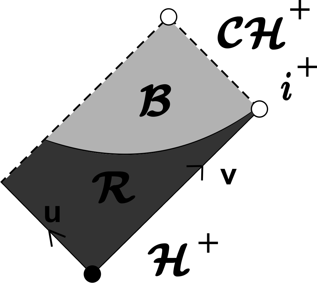
Figure 2: Penrose diagram illustrating the division between a red-shift $\mathcal{R}$ and a blue-shift region $\mathcal{B}$.

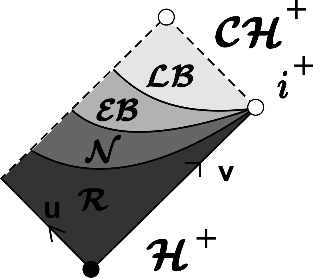
Figure 3: Penrose diagram of the space-time $\mathcal{M}=\mathcal{R}\cup\mathcal{N}\cup\mathcal{EB}\cup\mathcal{LB}$

In our case, we follow a similar philosophy although we need to further divide the space-time into more regions in view of the slow decay of the scalar field c.f Figure 3.

In the red-shift region, decay is proven using that $|\frac{-4\partial_{u}r}{\Omega^{2}}-1|$ and $|\frac{-4\partial_{v}r}{\Omega^{2}}-1|$ decay polynomially , thanks to the Raychaudhuri equations, which allows us to replace $\partial_{v}r$ and $\partial_{u}r$ by $\Omega^{2}\backsimeq e^{2K_{+}\cdot(u+v)}$ which enjoys an exponential structure. This avoids to lose one power when we integrate a polynomial decay on a large region c.f Lemma 4.1.

In the blue-shift region, we essentially use the polynomial decay of $\partial_{v}r$, $\partial_{u}r$ and the exponential decay of $\Omega^{2}$ to propagate the estimates.

Another important point is that we are able to find two decaying quantities which capture the red and blue shift effect : $\partial_{u}\log(\Omega^{2})-2K$ and $\partial_{v}\log(\Omega^{2})-2K$ -where $K$ is a geometric quantity defined by (2.12) - and we control the sign of $K$ : positive in the red-shift region, negative in the blue-shift region.

In particular the good control of $\partial_{v}\log(\Omega^{2})-2K$ can be fruitfully integrated to control the smallness of $\Omega^{2}$ according to the different regions but requires a bit of care close to the Cauchy horizon where $\partial_{v}\log(\Omega^{2})-2K$ is no longer integrable in general.

To sum up, unlike the strategy of [26] which purely deals with differences whose decay is propagated like a wave, we mainly use propagative arguments for the scalar field only and rely on the geometry of the space-time and on the Raychaudhuri equations (2.17), (2.18) to prove our estimates.

1.3.2 Methods for the instability part

The first instability result is due to Dafermos in [14]. Like its stability counterpart, it relies crucially on the special structure of the equation and notably a very specific monotonicity property that does not hold in the presence of a massive or charged scalar field.

The work [26] also proves an instability statement. Nevertheless both the presence of the mass or of the charge also destroy the main argument. Indeed the argument makes use of an almost conservation law for the scalar field stress-energy tensor $\mathbb{T}^{SF}$. With a non-zero mass, a new term appears (c.f (1.3)) which has the wrong sign and cannot be easily controlled. If the field is charged, this time the two conservation laws -previously independent- coming from $\mathbb{T}^{SF}$ and $\mathbb{T}^{EM}$ are now coupled and therefore Luk and Oh’s method does not apply.

Instead, we borrow ideas from a paper of Luk and Sbierski [29] in which the authors prove the linear instability of Kerr’s interior. They simplify their methods and adapt them to the Reissner-Nordström case in an introductory section. The point is essentially to prove the blow-up of $\partial_{V}\phi$ on a constant $u$ hypersurface close to the Cauchy horizon, where $(u,V)$ is a regular coordinate system near the Cauchy horizon thanks to a polynomial lower bound on $\int_{v}^{+\infty}|\partial_{v}\phi|^{2}(u,v^{\prime})dv^{\prime}$ .

For this they use an integrated $L^{2}$ stability estimate coupled with a vector field method - namely an energy estimate- using the Killing vector field $\partial_{t}=\partial_{v}-\partial_{u}$ -which boils down to the conservation of the energy. They manage to control the integral of $\partial_{v}\phi$ on the event horizon by its values on an intermediate curve $\gamma_{\sigma}$ (which marks the limit between their red-shift and their blue-shift region) on which $\Omega^{2}$ decays polynomially like $v^{-\sigma}$ for a very large power $\sigma>0$.

After they control this value by the integral of $\partial_{v}\phi$ on a constant $u$ hypersurface close to the Cauchy horizon using again a vector field method with the vector field $\partial_{v}$. They conclude using the positivity of the energy which allows for the $\partial_{v}$ terms to control the $\partial_{t}=\partial_{v}-\partial_{u}$ ones on $\gamma_{\sigma}$.

Their approach relies on the linearity of the problem and in particular the use of a Killing vector field of the Reissner-Nordström background , which does not exist any more in the non-linear setting that we consider.

Another important difference is the existence -in the uncharged field case- of two independent (approximate) conservation laws, namely one for the scalar field $\mathbb{T}^{SF}$ -which the authors of [29] use- and one for the electromagnetic field $\mathbb{T}^{EM}$ - which they ignore. In our case the charged field interacts with the charge of the black hole coupling the Klein-Gordon and the Maxwell equation. This gives a single (approximate) conservation law involving $\mathbb{T}=\mathbb{T}^{KG}+\mathbb{T}^{EM}$.

Moreover, the use of a vector field method in a blue-shift region for a charged and massive scalar field generates terms which do not decay, in particular those related to the charge of the black hole $Q$ and which have the inadequate sign.

Fortunately in the red-shift region the charge terms have a good sign and the estimates of our stability part are strong enough to prove decay of the scalar field terms having the wrong sign.

Moreover, despite Killing vector fields do not exist in general, the Kodama vector field $T$ -which is the non linear analog of $\partial_{t}$- induces a conservation law, which renders possible the use of a vector field method in the red-shift region.

There is however a difficulty : the coefficients of the Kodama vector field, unlike $\partial_{t}$, are expected to blow-up near the Cauchy horizon in general so the limiting curve $\gamma^{\prime}$ between the red-shift and the blue-shift region -unlike in [29]- must be close enough to the Cauchy horizon so that we enjoy a sufficient decay of $\Omega^{2}$ in the future to propagate the decay of the wave equations but must also be close enough to the event horizon so that the Kodama vector field does not blow-up ! Compared to [29] where the limiting curve was chosen to be as far as possible in the future, this is a completely different strategy.

This challenge is addressed using fine stability estimates, notably the quantities $\frac{-4\partial_{u}r}{\Omega^{2}}$ and $\frac{-4\partial_{v}r}{\Omega^{2}}$ which are precisely the coefficients of $T$ and that are controlled in the vicinity of $\gamma^{\prime}$.

In the blue-shift region, since vector field methods are now hard to use, we simply propagate point-wise $\partial_{v}\phi$ using the wave equation and the sufficient decay of $\Omega^{2}$ in the future of $\gamma^{\prime}$. We strongly rely on the stability estimates proven in the first part.

Lastly, once this lower bound is proven, we use exactly and without modifications the techniques employed in [26] to prove the blow-up of a $C^{2}$ geometric invariant quantity for any $s>\frac{1}{2}$ and the $H^{1}$ blow up of the scalar field if $s>1$, leading to the $C^{1}$ inextendibility of the $C^{0}$ extension constructed in the stability part.

1.4 Outline of the paper

We conclude this introduction by presenting the rest of the article.

Section 2 is devoted to preliminaries : we notably define the main notations, introduce the equations and express them in the form that we use later. A brief review of the Reissner-Nordström background is also presented.

In section 3, we phrase the main results of the paper precisely, namely the stability and the instability theorems. They are preceded by a reminder on the characteristic initial value problem and the coordinate dependency.

In section 4, the proof of the stability theorem is carried on. The proof of one minor proposition is deferred to appendix B and a simple local existence lemma is proven in appendix C

In section 5, the proof of the instability theorem is carried on.

Finally, in the appendix A, we use our stability framework to “localise” in coordinates the part of the apparent horizon that is close to time-like infinity.

1.5 Acknowledgements

I would like to express my deepest gratitude to my PhD advisor Jonathan Luk for suggesting this problem, for his continuous enlightening guidance, for his precious advice, his patience and for his invaluable help to work in good conditions.

My special thanks go to Haydée Pacheco for her crucial graphical contribution, namely drawing the Penrose diagrams.

I also would like to thank two anonymous referees for valuable suggestions.

I gratefully acknowledge the financial support of the EPSRC, grant reference number EP/L016516/1.

This work was completed while I was a visiting student in Stanford university and I gratefully acknowledge their financial support.

2 Geometric framework and equations

2.1 The equations in geometric form

We look for solutions to the Einstein-Maxwell equations coupled with a charged and massive scalar field $\phi$ of constant mass $m^{2}\geq 0$ and constant charge $q_{0}\neq 0$ propagating according to the Klein-Gordon equation in curved space-time :

A solution is described by a quadruplet $(M,g,\phi,F)$ - where $(M,g)$ is a Lorentzian manifold of dimension $3+1$, $\phi$ is a complex-valued function on $M$ and $F$ is a real-valued 2-form on $M$ - which satisfies the following equations :

$$Ric_{\mu\nu}(g)-\frac{1}{2}R(g)g_{\mu\nu}=\mathbb{T}^{EM}_{\mu\nu}+\mathbb{T}^{KG}_{\mu\nu},$$ (2.1)

$$\mathbb{T}^{EM}_{\mu\nu}=2\left(g^{\alpha\beta}F_{\alpha\nu}F_{\beta\mu}-\frac{1}{4}F^{\alpha\beta}F_{\alpha\beta}g_{\mu\nu}\right),$$ (2.2)

$$\mathbb{T}^{KG}_{\mu\nu}=2\left(\Re(D_{\mu}\phi\overline{D_{\nu}\phi})-\frac{1}{2}(g^{\alpha\beta}D_{\alpha}\phi\overline{D_{\beta}\phi}+m^{2}|\phi|^{2})g_{\mu\nu}\right),$$ (2.3)

$$\nabla^{\mu}F_{\mu\nu}=\frac{q_{0}}{2}i(\phi\overline{D_{\nu}\phi}-\overline{\phi}D_{\nu}\phi),\;F=dA,$$ (2.4)

$$g^{\mu\nu}D_{\mu}D_{\nu}\phi=m^{2}\phi,$$ (2.5)

where $D:=\nabla+iq_{0}A$ is the gauge derivative, $\nabla$ is the Levi-Civita connection of $g$ and $A$ is the potential one-form . $\mathbb{T}^{EM}_{\mu\nu}$ and $\mathbb{T}^{KG}_{\mu\nu}$ are the electromagnetic and the Klein-Gordon stress-energy tensor respectively.

(2.1) is the Einstein equation, (2.4) is the Maxwell equation and (2.5) is the Klein-Gordon equation. Note that they are all coupled one to another.

2.2 Metric in null coordinates, mass, charge and main notations

Let $(M,g,\phi,F)$ be a spherically symmetric solution of the Einstein-Maxwell-Klein-Gordon equations. By this we mean that $SO(3)$ acts on $(M,g)$ by isometry with spacelike orbits and for all $R_{0}\in SO(3)$, the pull-back of $F$ and $\phi$ by $R_{0}$ coincides with itself.

We define $\mathcal{Q}=M/SO(3)$, the quotient 2-dimensional manifold induced by the action of $SO(3)$.

$\Pi:M\rightarrow\mathcal{Q}$ is the canonical projection taking a point of $M$ into its spherical orbit.

The metric on $M$ is then given by $g=g_{\mathcal{Q}}+r^{2}d\sigma_{\mathbb{S}^{2}}$ where $g_{\mathcal{Q}}$ is the push-forward of $g$ by $\Pi$ and $d\sigma_{\mathbb{S}^{2}}$ the standard metric on the sphere.

$g_{\mathcal{Q}}$ as a general Lorentzian metric over a 2-dimensional manifold, can be written in null coordinates $(u,v)$ as a conformally flat metric :

$$g_{\mathcal{Q}}:=-\frac{\Omega^{2}}{2}(du\otimes dv+dv\otimes du).$$

We define the area-radius function $r$ over $\mathcal{Q}$ by $r(p)=\sqrt{\frac{Area(\Pi^{-1}(p))}{4\pi}}$.

We can then define $\kappa$ and $\iota$ as :

$$\kappa=\frac{-\Omega^{2}}{4\partial_{u}r}\in\mathbb{R}\cup\{\pm\infty\},$$ (2.6)

$$\iota=\frac{-\Omega^{2}}{4\partial_{v}r}\in\mathbb{R}\cup\{\pm\infty\}.$$ (2.7)

Remark 7.

Notice that $\kappa$ is invariant under $u$-coordinate change : if $du^{\prime}=f(u)du$, then in the new coordinate system $(u^{\prime},v)$, $\kappa(u^{\prime},v)=\kappa(u,v)$. Similarly , $\iota$ is invariant under $v$-coordinate change.

We can also define the Hawking mass and mass ratio as geometric quantities, at least in spherical symmetry :

$$\rho:=\frac{r}{2}(1-g_{\mathcal{Q}}(\nabla r,\nabla r)),$$

$$\mu:=\frac{2\rho}{r}.$$

In what follows, we will abuse notation and denote by $F$ the 2-form over $\mathcal{Q}$ that is the push-forward by $\Pi$ of the electromagnetic 2-form originally on $M$, and same for $\phi$.

It turns out that spherical symmetry allows us to set :

$$F=\frac{Q}{2r^{2}}\Omega^{2}du\wedge dv,$$

where $Q$ is a scalar function that we call the electric charge.

Remark 8.

It should be noted that in the Einstein-Maxwell-Scalar-Field of [14] and [26], $Q\equiv e$ was forced to be a constant because it was coupled with vacuum Maxwell’s equation $div\;F=0$.

$F=dA$ also allows us to chose a spherically symmetric potential $A$ written as :

$$A=A_{u}du+A_{v}dv.$$

The equations of section 2.1 are invariant under the following gauge transformation :

$$\phi\rightarrow e^{-iq_{0}f}\phi,$$

$$A\rightarrow A+df.$$

where $f$ is a smooth real-valued function.

Therefore we can choose the following gauge for some constant $v_{0}$ and for all $(u,v)$ :

$$A_{v}(u,v)\equiv 0,$$ (2.8)

$$A_{u}(u,v_{0})=0.$$ (2.9)

Remark 9.

Notice that this gauge depends only on the null foliation and therefore is invariant if $u$ or $v$ is re-parametrized.

This gauge will be used in the rest of the paper, for $v_{0}$ to be specified in the statement of Theorem 3.2.

For a more justified and complete discussion of the Einstein-Maxwell-Klein-Gordon setting, c.f [23].

Now we introduce the modified mass $\varpi$ that takes the charge $Q$ into account :

$$\varpi:=\rho+\frac{Q^{2}}{2r}=\frac{\mu r}{2}+\frac{Q^{2}}{2r}.$$ (2.10)

An elementary computation relates coordinate-dependent quantities to geometric ones :

$$1-\mu=\frac{-4\partial_{u}r\partial_{v}r}{\Omega^{2}}=\frac{-\Omega^{2}}{4\iota\kappa}=1-\frac{2\varpi}{r}+\frac{Q^{2}}{r^{2}}.$$ (2.11)

We then define the geometric quantity $2K$ :

$$2K=\frac{2}{r^{2}}(\varpi-\frac{Q^{2}}{r}).$$ (2.12)

We will also denote, for fixed constants $M$ and $e$ :

$$2K_{M,e}(r)=\frac{2}{r^{2}}(M-\frac{e^{2}}{r}).$$

Finally we introduce the following notation, first used by Christodoulou :

$$\lambda=\partial_{v}r,$$

$$\nu=\partial_{u}r.$$

2.3 The Reissner-Nordström solution

In this section we present the sub-extremal Reissner-Nordström solution. Because the space-time that we consider converges at late time towards a member of the Reissner-Nordström family and that we aim at proving stability estimates, it is important to recall their main qualitative features to see which are conserved in the presence of a perturbation.

2.3.1 The Reissner-Nordström interior metric

The Reissner-Nordström black hole is a 2-parameter family of spherically symmetric and static space-times indexed by the charge and the mass $(e,M)$, which satisfy the Einstein-Maxwell equations i.e the system of section 2.1 with $\phi\equiv 0$ with $\mathbb{R}_{+}^{*}\times\mathbb{S}^{2}$ initial data.

We are interested in sub-extremal Reissner-Nordström black holes, which is expressed by the condition $0<|e|<M$.

Define then for such $(e,M)$ :

$$r_{+}(M,e)=M+\sqrt{M^{2}-e^{2}}>0,$$

$$r_{-}(M,e)=M-\sqrt{M^{2}-e^{2}}>0.$$

The metric in the interior of the black hole can be written in coordinates as :

$$g_{RN}=\frac{\Omega^{2}_{RN}}{4}dt^{2}-4\Omega^{-2}_{RN}dr^{2}+r^{2}[d\theta^{2}+\sin(\theta)^{2}d\psi^{2}],$$ (2.13)

$$\Omega^{2}_{RN}(r):=-4(1-\frac{2M}{r}+\frac{e^{2}}{r^{2}}),$$ (2.14)

Where $(r,t,\theta,\psi)\in(r_{-},r_{+})\times\mathbb{R}\times[0,\pi)\times[0,2\pi]$ .

2.3.2 $(u,v)$ coordinate system on Reissner-Nordström background

We have seen in Section 2.2 how to build any null coordinate $(u,v)$. Now that the metric is explicit, we would like to find such a $(u,v)$ system that is related to the variables $(r,t)$ appearing in equation (2.13).

Define

$$r^{*}=r+\frac{1}{2K_{+}}\log(r_{+}-r)+\frac{1}{2K_{-}}\log(r-r_{-}),$$

where $2K_{+}(M,e)$ and $2K_{-}(M,e)$, respectively called the surface gravity of the event horizon and the surface gravity of the Cauchy horizon, are defined by :

$$K_{+}(M,e)=\frac{1}{r_{+}^{2}}(M-\frac{e^{2}}{r_{+}})=\frac{r_{+}-r_{-}}{2r_{+}^{2}}>0,$$

$$K_{-}(M,e)=\frac{1}{r_{-}^{2}}(M-\frac{e^{2}}{r_{-}})=\frac{r_{-}-r_{+}}{2r_{-}^{2}}<0.$$

Remark 10.

Note that if $\varpi=M$ and $Q=e$ then $K(r_{+})=K_{+}(M,e)>0$ and $K(r_{-})=K_{-}(M,e)<0$, where $K$ is defined in equation (2.12).

We then set $(u,v)\in\mathbb{R}\times\mathbb{R}$ as :

$$v=\frac{1}{2}(r^{*}+t),\,u=\frac{1}{2}(r^{*}-t),$$

and claim that equation (2.13) can then be rewritten as :

$$g_{RN}=-\frac{\Omega^{2}_{RN}}{2}(du\otimes dv+dv\otimes du)+r^{2}[d\theta^{2}+\sin(\theta)^{2}d\psi^{2}].$$

2.3.3 Behaviour of $\Omega^{2}_{RN}$

We define the event horizon $\mathcal{H}^{+}=\{u\equiv-\infty,v\in\mathbb{R}\}$, and the Cauchy horizon $\mathcal{CH}^{+}=\{v\equiv+\infty,u\in\mathbb{R}\}$

$\Omega^{2}_{RN}$ cancels on both $\mathcal{H}^{+}$ and $\mathcal{CH}^{+}$. A computation shows that :

$$\Omega^{2}_{RN}\sim_{r\rightarrow r_{+}}C_{e,M}e^{2K_{+}r^{*}}=C_{e,M}e^{2K_{+}\cdot(u+v)},$$

and similarly that :

$$\Omega^{2}_{RN}\sim_{r\rightarrow r_{-}}C^{\prime}_{e,M}e^{2K_{-}r^{*}}=C^{\prime}_{e,M}e^{2K_{-}\cdot(u+v)},$$

for some $C_{e,M}>0$, $C_{e,M}^{\prime}>0$.

Remark 11.

Notice that $\Omega^{2}_{RN}$ exhibits an exponential behaviour in $(u+v)$, exponentially increasing from 0 near the event horizon and exponentially decreasing to 0 near the Cauchy horizon.

Notice also that for $r$ bounded away from $r_{+}$ and $r_{-}$, $\Omega^{2}_{RN}$ is upper and lower bounded.

2.3.4 Kruskal coordinates $(U,V)$ and Eddington-Finkelstein coordinates $(U,v)$, $(u,V)$

From the previous section, one could fear that the metric could be singular across the horizons $\mathcal{H}^{+}$ and $\mathcal{CH}^{+}$. Actually it is not : like for the Scharwzchild’s event horizon horizon, it suffices to define Kruskal-like coordinates $(U,V)$ from the $(u,v)$ coordinates as :

$$U:=\frac{1}{2K_{+}}e^{2K_{+}u},$$

and

$$V:=1-\frac{1}{2|K_{-}|}e^{2K_{-}v}.$$

Note that $U$ and $V$ now range in $(U,V)\in[0,+\infty)\times(-\infty,1]$ and that $\mathcal{H}^{+}=\{U\equiv 0\}$ ; $\mathcal{CH}^{+}=\{V\equiv 1\}$.

We then write the metric in the Eddington-Finkelstein-type mixed $(U,v)$ coordinates as :

$$g_{RN}:=-\frac{\Omega^{2}_{RN,H}}{2}(dU\otimes dv+dv\otimes dU)+r^{2}[d\theta^{2}+\sin(\theta)^{2}d\psi^{2}].$$

We find that $(U,v)$ is a regular coordinate system near the event horizon $\mathcal{H}^{+}$ :

$$\Omega^{2}_{RN,H}(U,v)=-\frac{1}{2K_{+}U}(1-\frac{2M}{r}+\frac{e^{2}}{r^{2}})\rightarrow_{U\rightarrow 0}C_{e,M}e^{2K_{+}v}.$$

In $(u,V)$ coordinates we write now write the metric as :

$$g_{RN}:=-\frac{\Omega^{2}_{RN,CH}}{2}(du\otimes dV+dV\otimes du)+r^{2}[d\theta^{2}+\sin(\theta)^{2}d\psi^{2}].$$

We then see that $(u,V)$ is a regular coordinate system near the Cauchy horizon $\mathcal{CH}^{+}$ :

$$\Omega^{2}_{RN,CH}(u,V)=\frac{1}{2K_{-}(1-V)}(1-\frac{2M}{r}+\frac{e^{2}}{r^{2}})\rightarrow_{V\rightarrow 1}C_{e,M}^{\prime}e^{-2K_{-}u}.$$

2.3.5 Constant quantities on Reissner-Nordström

Since we consider the stability of a Reissner-Nordström background under perturbation, it is useful to identify which quantities are zero on this fixed background : these are the ones that we can hope decay for in the non-linear perturbative setting with the Klein-Gordon field.

Reissner-Nordstörm has four main qualitative features which distinguishes it from general dynamical solutions :

1. Both the charge and the modified mass are fixed :

   $$\varpi\equiv M,$$

   $$Q\equiv e.$$

   Hence $1-\mu=1-\frac{2M}{r}+\frac{e^{2}}{r^{2}}$.

2. The metric is symmetric in $u$ and $v$ and in particular :

   $$\partial_{u}r=\partial_{v}r,$$

   $$\partial_{u}\log(\Omega^{2}_{RN})=\partial_{v}\log(\Omega^{2}_{RN})=\frac{2}{r^{2}}(M-\frac{e^{2}}{r})=2K_{M,e}(r).$$

3. The horizons are constant $r$ null hypersurfaces :

   $$\mathcal{H}^{+}=\{u\equiv-\infty,v\in\mathbb{R}\}=\{r\equiv r_{+}\},$$

   $$\mathcal{CH}^{+}=\{v\equiv+\infty,u\in\mathbb{R}\}=\{r\equiv r_{-}\}.$$

   Hence $\partial_{v}r_{|\mathcal{H}^{+}}\equiv 0$ and $\partial_{u}r_{|\mathcal{CH}^{+}}\equiv 0$ which is consistent with the following relation :

   $$\partial_{u}r=\partial_{v}r=1-\frac{2M}{r}+\frac{e^{2}}{r^{2}}.$$

4. The event horizon $\mathcal{H}^{+}$ coincides with the apparent horizon $\mathcal{A}:=\{\partial_{v}r=0\}$ so all the 2-spheres inside the black hole are trapped.

   This does not hold for general dynamical space-times where $\mathcal{A}$ is strictly in the future of $\mathcal{H}^{+}$.

   However, in the perturbative regime, we can expect that $\mathcal{A}$ is not too far from $\mathcal{H}^{+}$, c.f Appendix A.

In the end, we can sum up all the relations by :

$$\partial_{u}r=\partial_{v}r=1-\frac{2M}{r}+\frac{e^{2}}{r^{2}}=-\frac{\Omega^{2}_{RN}}{4}\leq 0,$$

which also means that :

$$\kappa_{RN}=\iota_{RN}\equiv 1.$$

2.4 The Einstein-Maxwell-Klein-Gordon equations in null coordinates

Finally, we express the Einstein-Maxwell-Klein-Gordon system in spherical symmetry in any (u,v) coordinates as in section 2.2 and under the gauge choice for the potential (2.8), (2.9).

We start by the wave part of the Einstein equation :

$$\partial_{u}\partial_{v}r=\frac{-\Omega^{2}}{4r}-\frac{\partial_{u}r\partial_{v}r}{r}+\frac{\Omega^{2}}{4r^{3}}Q^{2}+\frac{m^{2}r}{4}\Omega^{2}|\phi|^{2}=-\frac{\Omega^{2}}{4}.2K+\frac{m^{2}r}{4}\Omega^{2}|\phi|^{2},$$ (2.15)

$$\partial_{u}\partial_{v}\log(\Omega^{2})=-2\Re(D_{u}\phi\partial_{v}\bar{\phi})+\frac{\Omega^{2}}{2r^{2}}+\frac{2\partial_{u}r\partial_{v}r}{r^{2}}-\frac{\Omega^{2}}{r^{4}}Q^{2},$$ (2.16)

the Raychaudhuri equations :

$$\partial_{u}(\frac{\partial_{u}r}{\Omega^{2}})=\frac{-r}{\Omega^{2}}|D_{u}\color[rgb]{0,0,0}\phi|^{2},$$ (2.17)

$$\partial_{v}(\frac{\partial_{v}r}{\Omega^{2}})=\frac{-r}{\Omega^{2}}|\partial_{v}\color[rgb]{0,0,0}\phi|^{2},$$ (2.18)

the Klein-Gordon wave equation :

$$\partial_{u}\partial_{v}\phi=-\frac{\partial_{u}\phi\partial_{v}r}{r}-\frac{\partial_{u}r\partial_{v}\phi}{r}+\frac{q_{0}i\Omega^{2}}{4r^{2}}Q\phi-\frac{m^{2}\Omega^{2}}{4}\phi-iq_{0}A_{u}\frac{\phi\partial_{v}r}{r}-iq_{0}A_{u}\partial_{v}\phi,$$ (2.19)

and the propagative part of Maxwell’s equation :

$$\partial_{u}Q=-q_{0}r^{2}\Im(\phi\overline{D_{u}\phi}).$$ (2.20)

$$\partial_{v}Q=q_{0}r^{2}\Im(\phi\overline{\partial_{v}\phi}).$$ (2.21)

Also the existence of an electro-magnetic potential $A$ implies that :

$$\partial_{v}A_{u}=\frac{-Q\Omega^{2}}{2r^{2}}.$$ (2.22)

Now we can reformulate the former equations to put them in a form that is more convenient to use.

It is interesting to use (2.15), (2.17), (2.18), (2.20), (2.21) to derive an equation for the modified mass :

$$\partial_{u}\varpi=\frac{r^{2}}{2\iota}|D_{u}\color[rgb]{0,0,0}\phi|^{2}+\frac{m^{2}}{2}r\partial_{u}r|\phi|^{2}-i\frac{q_{0}}{2}Qr\Im(\bar{\phi}D_{u}\phi),$$ (2.23)

$$\partial_{v}\varpi=\frac{r^{2}}{2\kappa}|\partial_{v}\phi|^{2}+\frac{m^{2}}{2}r\partial_{v}r|\phi|^{2}+i\frac{q_{0}}{2}Qr\Im(\bar{\phi}\partial_{v}\phi).$$ (2.24)

Moreover, the following reformulation of (2.15) will be useful :

$$\partial_{v}\log(|\partial_{u}r|)=\kappa(2K-rm^{2}|\phi|^{2}).$$ (2.25)

Remark 12.

Note that the left-hand-side, like $\kappa$ is invariant under u-coordinate changes.

We also reformulate (2.16) as :

$$\partial_{u}\partial_{v}\log(\Omega^{2})=\kappa\partial_{u}(2K)-2\Re(D_{u}\phi\partial_{v}\bar{\phi})-\frac{2\kappa}{r^{2}}(\partial_{u}\varpi-\frac{\partial_{u}Q^{2}}{r})=\\ \iota\partial_{v}(2K)-2\Re(D_{u}\phi\partial_{v}\bar{\phi})-\frac{2\iota}{r^{2}}(\partial_{v}\varpi-\frac{\partial_{v}Q^{2}}{r}).$$ (2.26)

We can also rewrite (2.19) to control $|\partial_{v}\phi|$ more easily :

$$e^{-iq_{0}\int_{u_{0}}^{u}A_{u}}\partial_{u}(e^{iq_{0}\int_{u_{0}}^{u}A_{u}}\partial_{v}\phi)=-\frac{\partial_{v}rD_{u}\phi}{r}-\frac{\partial_{u}r\partial_{v}\phi}{r}+\frac{q_{0}i\Omega^{2}}{4r^{2}}Q\phi-\frac{m^{2}\Omega^{2}}{4}\phi,$$ (2.27)

or to control $|D_{u}\phi|$ more easily :

$$\partial_{v}(D_{u}\phi)=-\frac{\partial_{u}r\partial_{v}\phi}{r}-\frac{\partial_{v}rD_{u}\phi}{r}-\frac{m^{2}\Omega^{2}}{4}\phi.$$ (2.28)

Finally we can also write the Raychaudhuri equations as :

$$\partial_{u}(\kappa^{-1})=\frac{4r}{\Omega^{2}}|D_{u}\color[rgb]{0,0,0}\phi|^{2},$$ (2.29)

$$\partial_{v}(\iota^{-1})=\frac{4r}{\Omega^{2}}|\partial_{v}\color[rgb]{0,0,0}\phi|^{2}.$$ (2.30)

3 Precise statement of the main results

3.1 Preliminaries on characteristic initial value problem and coordinate choice

Before stating the theorem, we want to demystify a little the framework used to define the gauges and the coordinate dependent objects. The context is the same as for [14] and [26] , the only difference is the presence of the (dynamical) charge of the space-time $Q$.

We want to phrase the characteristic initial value problem for the Einstein-Maxwell-Klein-Gordon system of section 2.1. The reader familiar with the framework can skip this section.

We first consider two connected and oriented smooth, 1-dimensional manifolds $\mathcal{C}_{in}$ and $\mathcal{C}_{out}$ -each with a boundary point (c.f Figure 1.)

We can identify the surfaces at their boundary point to get $\mathcal{C}_{in}\cup_{\{p\}}\mathcal{C}_{out}$, on which we now want to build a $(U,v)$ null regular coordinate system. For this, we have four choices to make :

1. Choosing an increasing parametrization $U$ of $\mathcal{C}_{in}$.

2. Choosing an increasing parametrization $v$ of $\mathcal{C}_{out}$.

3. Choosing the $U$-coordinate $U_{0}\in\mathbb{R}\cup\{\pm\infty\}$ of the intersection point p.

4. Choosing the $v$-coordinate $v_{0}\in\mathbb{R}\cup\{\pm\infty\}$ of the intersection point p.

In this coordinate system, $\mathcal{C}_{in}$ and $\mathcal{C}_{out}$ can be written as :

$$\mathcal{C}_{in}=\{(U,v_{0}),U\in[U_{0},U_{max})\},$$

$$\mathcal{C}_{out}=\{(U_{0},v),v\in[v_{0},v_{max})\},$$

with $U_{max}\in\mathbb{R}\cup\{\pm\infty\}$, $v_{max}\in\mathbb{R}\cup\{\pm\infty\}$.

As our initial data we shall consider $(r,\Omega^{2}_{H},\phi,A)$ as follows :

$(r,\phi)$ are $C^{1}$ scalar functions and $A$ a $C^{1}$ 1-form on $\mathcal{C}_{in}\cup_{\{p\}}\mathcal{C}_{out}$.

$r$ and $\phi$ induce -in the $(U,v)$ coordinate system- some functions on $[v_{0},v_{max})\times\{U_{0}\}\cup\{v_{0}\}\times[U_{0},U_{max})$ that we still call $r$ and $\phi$ by notation abuse.

$A$ induces a function $A_{v}$ on $[v_{0},v_{max})\times\{u_{0}\}$ by $A_{|C_{out}}=A_{v}dv$ and another function $A_{U}$ on $\{v_{0}\}\times[U_{0},U_{max})$ by $A_{|C_{in}}=A_{U}dU$.

The remaining part of the data will be a $C^{1}$ function $\Omega^{2}_{H}:[v_{0},v_{max})\times\{u_{0}\}\cup\{v_{0}\}\times[U_{0},U_{max})\rightarrow\mathbb{R}_{+}^{*}$. We will use this later to build a metric of the form $g=-\frac{\Omega^{2}_{H}}{2}(dU\otimes dv+dv\otimes dU)++r^{2}[d\theta^{2}+\sin(\theta)^{2}d\psi^{2}]$.

The prescription of $\Omega^{2}_{H}$ as above will be coordinate dependent.

This coordinate dependent framework allows us to define the Raychaudhuri equations on the initial surfaces, seen as constraints for the characteristic initial value problem.

However, they are still valid under any re-parametrization of $U$ or $v$ :

Definition 1 (Raychaudhuri equations).

We say that the data $(r,\Omega^{2}_{H},\phi,A)$ satisfy the Raychaudhuri equations if on $\{v_{0}\}\times[U_{0},U_{max})$ :

$$\partial_{U}(\frac{\partial_{U}r}{\Omega^{2}_{H}})=\frac{-r}{\Omega^{2}_{H}}|D_{U}\phi|^{2}.$$

And on $[v_{0},v_{max})\times\{U_{0}\}$ :

$$\partial_{v}(\frac{\partial_{v}r}{\Omega^{2}_{H}})=\frac{-r}{\Omega^{2}_{H}}|D_{v}\phi|^{2},$$

where $D$ depends on $A$ by $D=\partial+iq_{0}A$ as an operator on scalar functions.

We now want to talk of “the solution” - up to gauge transforms- of the Einstein-Maxwell-Klein-Gordon equations. To do so, we solve the partial differential equation system of section 2.4 “abstractly” for some data $(r,\Omega^{2},\phi,A)$. Since it is standard that the Raychaudhuri equations -once satisfied on the initial surfaces- are propagated, we see the solution actually satisfies the Einstein-Maxwell-Klein-Gordon equations in their geometric form of section 2.1.

Theorem 3.1 (Characteristic initial value problem).

Let $\mathcal{C}_{in}$, $\mathcal{C}_{out}$ be as before.

We assume moreover that the data $(r,\Omega^{2}_{H},\phi,A)$ are as before and satisfy the Raychaudhuri equations. Moreover we suppose that $r>0$.

Then there exists a unique $C^{1}$ maximal globally hyperbolic development $(M,g,\phi,F)$, spherically symmetric solution of Einstein-Maxwell-Klein-Gordon equations of section 2.1 such that

1. $\mathcal{C}_{out}$ and $\mathcal{C}_{in}$ embed into $\mathcal{Q}=\mathcal{M}/SO(3)$ as null boundaries with respect to the metric $g$.

2. $D^{+}(\mathcal{C}_{in}\cup_{\{p\}}\mathcal{C}_{out})\cap\mathcal{Q}=J^{+}({\{p\}})\cap\mathcal{Q}$

   where $D^{+}$ denotes the future domain of dependence and $J^{+}$ the causal future .

3. $(M,g,\phi,F)$ satisfy :

   $$g=-\frac{\Omega^{2}_{H}}{2}(dU\otimes dv+dv\otimes dU)+r^{2}[d\theta^{2}+\sin(\theta)^{2}d\psi^{2}],$$

   $$F=dA.$$

   And $(r,\Omega^{2}_{H},\phi,A)$ restrict on the initial surfaces to the value prescribed

   by the initial data $(r,\Omega^{2}_{H},\phi,A)_{|\mathcal{C}_{in}\cup_{\{p\}}\mathcal{C}_{out}}$.

4. The equations in null coordinates of section 2.4 are satisfied.

For a more thorough discussion of the uniqueness problem in that framework, c.f [12].

3.2 The stability theorem

We can now formulate the main stability theorem. The main point is the presence of a Cauchy horizon, reflected by the form of the Penrose diagram, instead of space-like Schwarzschild-type singularity.

Theorem 3.2 (Non-linear stability theorem).

Let $\mathcal{C}_{in}$, $\mathcal{C}_{out}$ and $(r,\phi,\Omega^{2}_{H},A)$ satisfy the assumptions of Theorem 3.1.

Moreover, we will make the following geometric assumptions :

Assumption 1.

$\mathcal{C}_{out}$ is affine complete .

Assumption 2.

$r>0$ is a strictly decreasing function on $\mathcal{C}_{in}$ with respect to any increasing parametrization.

From now on we will denote $\mathcal{H}^{+}:=\mathcal{C}_{out}$ and call $\mathcal{H}^{+}$ the event horizon.

For some constant $v_{0}>0$ , we parametrize $\mathcal{H}^{+}:=\mathcal{C}_{out}=\{U\equiv 0,v\geq v_{0}\}$ with a coordinate $v$ defined by

$$\kappa_{|\mathcal{H}^{+}}=(\frac{-\Omega^{2}_{H}(0,v)}{4\partial_{U}r(0,v)})_{|\mathcal{H}^{+}}\equiv 1,$$ (3.1)

and for some $U_{max}>0$, we parametrize $\mathcal{C}_{in}=\{v\equiv v_{0},0\leq U\leq U_{max},\}$ with a coordinate $U$ defined by

$$(\partial_{U}r)_{|\mathcal{C}_{in}}(U,v_{0})\equiv-1.$$ (3.2)

We also make the following no-anti-trapped surfaces assumption :

Assumption 3.

$\partial_{U}r(0,v)_{|\mathcal{H}^{+}}<0$

We assume the following decay on the field in $(U,v)$ coordinates : there exists $C>0$ and $s>\frac{1}{2}$ such that

Assumption 4.

$$|\phi(0,v)|_{|\mathcal{H}^{+}}+|\partial_{v}\phi(0,v)|_{|\mathcal{H}^{+}}\leq Cv^{-s},$$

Assumption 5.

$$|D_{U}\phi|(U,v_{0})\leq C.$$

We also ask the following convergences towards infinity on the event horizon :

Assumption 6.

$$r_{|\mathcal{H}^{+}}(0,v)\rightarrow r_{\infty}$$

as $v\rightarrow+\infty,$

where $r_{\infty}>0$ is a constant.

Assumption 7.

$$0<Q_{+}<r_{\infty},$$

where $Q_{+}:=\limsup_{v\rightarrow+\infty}|Q|_{|\mathcal{H}^{+}}$

We consider the unique $C^{1}$ maximal globally hyperbolic development $(M,g,\phi,F)$ of Theorem 3.1,

Then, after restriction to a small enough connected subset $p\in\mathcal{C}_{in}^{\prime}\subset\mathcal{C}_{in}$, i.e $\mathcal{C}_{in}^{\prime}=\{v\equiv v_{0},0\leq U\leq U_{s},\}$ for $0<U_{s}$ small enough, $D^{+}(\mathcal{C}_{in}^{\prime}\cup_{\{p\}}\mathcal{C}_{out})\cap\mathcal{Q}$ has the Penrose diagram of Figure 1.

Moreover, if $s>1$, $(M,g,\phi,F)$ admits a continuous extension to the Cauchy horizon.

More precisely, we can attach a future null boundary $\mathcal{CH}^{+}:=\{v\equiv+\infty,0\leq U\leq U_{s}\}$ to the space-time (M,g) such that $(g,\phi,F)$ each admits a continuous extension to the new space-time $\bar{M}:=M\cup\mathcal{CH}^{+}$ seen as a manifold with boundaries.

Remark 13.

Because of (2.11), (3.1) is exactly equivalent to :

$$\partial_{v}r_{|\mathcal{H}^{+}}=1-\frac{2\varpi}{r}+\frac{Q^{2}}{r^{2}}=1-\mu.$$ (3.3)

Remark 14.

The present paper introduces the first stability result dealing with all the possible values of $m^{2}$ and $q_{0}$. However the continuous extension statement when $s>1$ was already established in the work [14] and [26] although stated in the chargeless case $q_{0}=0$ only. Some continuous extension results for the charged case have also been proved in [23]. Notice (c.f section 1.2.2) that the case $s>1$ should be relevant in our context only if the scalar field is massless and not too charged compared to the black hole.

Remark 15.

Notice also that the assumptions are (almost) the same as those of [26], except for the strength of the decay rate, which was integrable unlike in the present paper.

In the rest of the paper, we will write $A\lesssim B$ if there exists a constant $\tilde{C}=\tilde{C}(C,Q_{+},q_{0},m^{2},r_{\infty},s,v_{0})$ such that $A\leq\tilde{C}B$.

If we need to specify this constant, we shall call it consistently $\tilde{C}$ when there are no ambiguities.

We denote also $A\sim B$ if $A\lesssim B$ and $B\lesssim A$.

3.3 The instability theorem

We can now phrase our instability theorem that relies very much on the non-linear stability claimed in the preceding section.

Theorem 3.3 (Non-linear instability theorem).

Let $\mathcal{C}_{in}$, $\mathcal{C}_{out}$ and $(r,\Omega^{2}_{H},\phi,A)$ satisfying all the assumptions of Theorem 3.2 and in particular assumption 4 with $s>\frac{1}{2}$.

We assume, using the same gauges as for Theorem 3.2, that the field in addition satisfies the following $L^{2}$ averaged polynomial lower-bound on the event horizon $C_{out}=\mathcal{H}^{+}$ :

Assumption 8.

$$v^{-p}\lesssim\int_{v}^{+\infty}|\partial_{v}\phi|^{2}_{|\mathcal{H}^{+}}(0,v^{\prime})dv^{\prime},$$ (3.4)

for $2s-1\leq p<\min\{2s,6s-3\}$.

Then for any $u\in\mathbb{R}$ negative enough, and for all $v$ large enough (depending on $u$),

$$\int_{v}^{+\infty}|\partial_{v}\phi|^{2}(u,v^{\prime})dv^{\prime}\gtrsim v^{-p}.$$ (3.5)

In particular the following component of the curvature blows-up on the Cauchy horizon :

$$\limsup_{v\rightarrow+\infty}Ric(\Omega^{-2}\partial_{v},\Omega^{-2}\partial_{v})(u,v)=+\infty.$$

Moreover for $s>1$, $\phi\notin W^{1,2}_{loc}$ and the metric is not $C^{1}$ for the continuous extension constructed in Theorem 3.2.

Remark 16.

This theorem is the very first instability result outside the uncharged and massless case. As explained in section 1.3.2, the methods of previous instability works do not apply here.

Remark 17.

In view of the result of [26], one can very reasonably hope that this curvature blow up leads to a $C^{2}$ inextendibility of the metric in an appropriate global setting . The reason for this is that $Ric(\Omega^{-2}\partial_{v},\Omega^{-2}\partial_{v})$ is a geometric quantity since $\Omega^{-2}\partial_{v}$ is a geodesic vector field. The only remaining argument is to extend the blow-up far from time-like infinity namely to get a global statement as opposed to perturbative.

4 Proof of the stability Theorem 3.2

We recall that we write $A\lesssim B$ if there exists a constant $\tilde{C}=\tilde{C}(C,Q_{+},q_{0},m^{2},r_{\infty},s,v_{0})$ such that $A\leq\tilde{C}B$.

If we need to specify this constant, we shall call it consistently $\tilde{C}$ when they are no ambiguities.

We denote also $A\sim B$ if $A\lesssim B$ and $B\lesssim A$.

When we write “with respect to the parameters”, we actually mean “with respect to $C$,$Q_{+}$,$q_{0}$,$m^{2}$,$r_{\infty}$ and $s$”.

We shall use repetitively the following technique : if we are in a region where $|u|\leq Dv$ where $D$ is a constant, then we can take $|u_{s}|$ large enough (equivalently $U_{s}$ small enough) so that for any $u\leq u_{s}$ and any function of $v$, $\epsilon(u,.)=o(1)$ where $v\rightarrow+\infty$ and any positive number $\eta$ then $|\epsilon(u,v)|\leq\eta$ for all $|u|\leq Dv$. When we do so, we write “for $|u_{s}|$ large enough” or equivalently in $(U,v)$ coordinates “for $U_{s}$ small enough”.

4.1 Strategy of the proof

The main idea of the proof is to split the space-time into smaller regions where the red-shift and blue-shift effect manifest themselves as already done in [14] and [26] and to integrate along the characteristic for the wave equations.

The main novelty is to deal with a non-integrable field decaying on $\mathcal{H}^{+}$ like $v^{-s}$ with $s>\frac{1}{2}$ only. The reason why stability estimates still proceed is that the Raychaudhuri equation on $\mathcal{H}^{+}$ involve the square of the field of the order $v^{-2s}$ which is integrable.

We will use five different regions :

1. The event horizon $\mathcal{H}^{+}:=\{U=0,v\geq v_{0}\}$ where we use crucially the Raychaudhuri equation and exhibit the right Reissner-Nordström space-time to which our dynamical space-time is expected to converge at infinity. We find that $\Omega^{2}$ behaves likes $e^{2K_{+}\cdot(u+v+h(v))}=2K_{+}Ue^{2K_{+}\cdot(v+h(v))}$ where $h(v)=o(v)$.

2. The red-shift region $\mathcal{R}=\{u+v+h(v)\leq-\Delta\}$: this is a large region where $\Omega^{2}$ is small enough and $|D_{u}\phi|\lesssim\Omega^{2}v^{-s}$. This strong stability feature is the key to prove the estimates. Another important feature is that $\Omega^{2}$ can almost be written as a product $f(u)\cdot g(v)$ which simplifies most of the calculations. This comes from the fact that $\Omega^{2}_{H}(U,v)$ is almost $\Omega^{2}_{H}(0,v)$, up to a arbitrary small constant $e^{-\tilde{C}\Delta}$.

3. The no-shift region $\mathcal{N}:=\{-\Delta\leq u+v+h(v)\leq\Delta_{N}\}$ : the function of this small region is to allow $r$ to vary from its event horizon limit value $r_{+}$ to its Cauchy horizon limit value $r_{-}$, up to arbitrarily small constants. The smallness of the region allows us to conserve the estimates of its past region $\mathcal{R}$ while initiating the blue-shift effect in its future.

4. The early blue-shift transition region $\mathcal{EB}:=\{\Delta_{N}\leq u+v+h(v)\leq-\Delta^{\prime}+\frac{2s}{2|K_{-}|}\log(v)\}$ : this small region is the first where the blue-shift happens and as a consequence the metric coefficients $\Omega^{2}(u,v)$ start to be small enough to facilitate the decay of propagating waves but do not decay too much so that we can still treat the problem as almost linear : in particular $\kappa^{-1}$ and $\iota^{-1}$ stay bounded.

5. The late blue-shift region $\mathcal{LB}:=\{-\Delta^{\prime}+\frac{2s}{2|K_{-}|}\log(v)\leq u+v+h(v)\}$ : this very large region exhibits the strongest blue-shift : the metric coefficients $\Omega^{2}(u,v)$ start from inverse polynomial decay but decrease exponentially in $v$ near the Cauchy horizon. We use this smallness to prove decay for the propagation problem. However, we do not prove enough decay to get a continuous extension of the space-time in the case $s\leq 1$.

The core of the proof is to control $\partial_{v}\log(\Omega^{2})$ and $\partial_{u}\log(\Omega^{2})$ and use Lemma 4.1 :

In $\mathcal{H}^{+}$ and $\mathcal{R}$, as a consequence of the red-shift effect, they are lower bounded by a strictly positive constant, which allows us to consider $\Omega^{2}$ as an increasing exponential in $u$ and as an increasing exponential in $v$, avoiding the loss of one power when we integrate a polynomial decay.

In $\mathcal{N}$, $\partial_{v}\log(\Omega^{2})$ and $\partial_{u}\log(\Omega^{2})$ change sign and can be close to $0$, but it does not matter for the decay of the scalar field because the region is small enough .

In $\mathcal{EB}$ and $\mathcal{LB}$, as a consequence of the blue-shift effect, they are upper bounded by a strictly negative constant, which allows us to consider $\Omega^{2}$ as a decreasing exponential in $u$ and as a decreasing exponential in $v$, which also avoids the loss of power when we integrate a polynomial decay.

4.2 A calculus lemma

We begin this proof section by a calculus lemma, which broadly says that integrating a polynomial decay -as expected for $\phi$- with a $\Omega^{2}$ or $\Omega^{-2}$ weight avoids to lose one power as we would otherwise.

Lemma 4.1.

Let $q\geq 0$, $a=a(e,M,q_{0},m^{2},s)>0$ and $\gamma_{1}$ be a one-dimensional curve on which $|u|\approx v$ with $u_{1}(v)$ being the only $u$ such that $(u,v)\in\gamma_{1}$ and $v_{1}(u)$ being the only $v$ such that $(u,v)\in\gamma_{1}$.

Then for any positive $C^{1}$ function $\Omega^{2}$, the following hold true :

1. Red-shift bounds in $|u|$ : assume that for all $u^{\prime}\in[u_{1}(v),u]$, $\partial_{u}\log(\Omega^{2})(u^{\prime},v)>a$. Then :

   $$\int_{u_{1}(v)}^{u}\Omega^{2}(u^{\prime},v)|u^{\prime}|^{-q}du^{\prime}\lesssim\Omega^{2}(u,v)|u|^{-q},$$

   $$\int_{u_{1}(v)}^{u}\Omega^{-2}(u^{\prime},v)|u^{\prime}|^{-q}du^{\prime}\lesssim\Omega^{-2}(u_{1}(v),v)v^{-q}.$$

2. Red-shift bounds in v : assume that for all $v^{\prime}\in[v_{1}(u),v]$, $\partial_{v}\log(\Omega^{2})(u^{\prime},v)>a$. Then :

   $$\int_{v_{1}(u)}^{v}\Omega^{2}(u,v^{\prime})v^{\prime-q}dv^{\prime}\lesssim\Omega^{2}(u,v)v^{-q}.$$

   $$\int_{v_{1}(u)}^{v}\Omega^{-2}(u,v^{\prime})v^{\prime-q}dv^{\prime}\lesssim\Omega^{-2}(u,v_{1}(u))|u|^{-q}.$$

3. Blue-shift bounds in $|u|$ : assume that for all $u^{\prime}\in[u_{1}(v),u]$, $\partial_{u}\log(\Omega^{2})(u^{\prime},v)<-a$. Then :

   $$\int_{u_{1}(v)}^{u}\Omega^{2}(u^{\prime},v)|u^{\prime}|^{-q}du^{\prime}\lesssim\Omega^{2}(u_{1}(v),v)v^{-q}.$$

   $$\int_{u_{1}(v)}^{u}\Omega^{-2}(u^{\prime},v)|u^{\prime}|^{-q}du^{\prime}\lesssim\Omega^{-2}(u,v)|u|^{-q}.$$

4. Blue-shift bounds in v : assume that for all $v^{\prime}\in[v_{1}(u),v]$, $\partial_{v}\log(\Omega^{2})(u^{\prime},v)<-a$. Then :

   $$\int_{v_{1}(u)}^{v}\Omega^{2}(u,v^{\prime})v^{\prime-q}dv^{\prime}\lesssim\Omega^{2}(u,v_{1}(u))|u|^{-q},$$

   $$\int_{v_{1}(u)}^{v}\Omega^{-2}(u,v^{\prime})v^{\prime-q}dv^{\prime}\lesssim\Omega^{-2}(u,v)v^{-q}.$$

Proof.

We will only prove one case when $\partial_{u}\log(\Omega^{2})>a$, the others being similar. For $u\geq u_{1}(v)$ :

$$\int_{u_{1}(v)}^{u}\Omega^{-2}(u^{\prime},v)|u^{\prime}|^{-q}du^{\prime}\leq\frac{1}{a}\int_{u_{1}(v)}^{u}\Omega^{-2}(u^{\prime},v)\partial_{u}\log(\Omega^{2})(u^{\prime},v)|u^{\prime}|^{-q}du^{\prime}=-\frac{1}{a}\int_{u_{1}(v)}^{u}\partial_{u}(\Omega^{-2})(u^{\prime},v)|u^{\prime}|^{-q}du^{\prime}.$$

Then we integrate by parts to write :

$$\int_{u_{1}(v)}^{u}\Omega^{-2}(u^{\prime},v)|u^{\prime}|^{-q}du^{\prime}\leq\frac{q}{a}\int_{u_{1}(v)}^{u}\Omega^{-2}(u^{\prime},v)|u^{\prime}|^{-q-1}du^{\prime}+\frac{1}{a}\Omega^{-2}(u_{1}(v),v)|u_{1}(v)|^{-q}-\frac{1}{a}\Omega^{-2}(u,v)|u|^{-q}.$$

Then clearly $\int_{u_{1}(v)}^{u}\Omega^{-2}(u^{\prime},v)|u^{\prime}|^{-q-1}du^{\prime}=o(\int_{u_{1}(v)}^{u}\Omega^{-2}(u^{\prime},v)|u^{\prime}|^{-q}du^{\prime})$ so the dominant term is the second, and $a$ depends on the parameters only, giving :

$$\int_{u_{1}(v)}^{u}\Omega^{-2}(u^{\prime},v)|u^{\prime}|^{-q}du^{\prime}\lesssim\Omega^{-2}(u_{1}(v),v)|u_{1}(v)|^{-q}.$$

∎

4.3 The event horizon

4.3.1 Convergence at infinity towards a Reissner-Nordström background

Proposition 4.2.

There exists constants $0<|e|<M$ such that on the event horizon $\mathcal{H}^{+}=\{U=0,v\geq v_{0}\}$

$$|\varpi(0,v)-M|\lesssim v^{1-2s},$$ (4.1)

$$|Q(0,v)-e|\lesssim v^{1-2s}.$$ (4.2)

And moreover $r_{\infty}=r_{+}(M,e)$ where $r_{\infty}$ is as in hypothesis 6 and

$$K(0,v)\rightarrow K_{+}(M,e)>0,$$

as $v\rightarrow+\infty$.

Proof.

First we use (2.21) together with the decay of assumption 4 and the boundedness of $r$ to get the existence of $e\in\mathbb{R}$ such that (4.2) holds. In particular $Q$ is bounded. Moreover, due to assumption 7, $e\neq 0$.

For the mass, notice that by integration by parts and the decay of assumption 4 :

$$|\int_{v}^{+\infty}r\partial_{v}r|\phi|^{2}dv^{\prime}|=|-\int_{v}^{+\infty}r^{2}\Re(\bar{\phi}\partial_{v}\phi)dv^{\prime}-\frac{r^{2}}{2}|\phi|^{2}(0,v)|\lesssim v^{1-2s}.$$

Therefore - the other terms being easier in (2.24)- by using gauge (3.1) and assumption 4, together with the boundedness of $r$, we prove that there exists $M\in\mathbb{R}$ such that (4.1) holds.

Gauge (3.1) then gives the following convergence when $v$ tends to $+\infty$ on $\mathcal{H}^{+}$ :

$$\partial_{v}r=1-\mu=1-\frac{2\varpi}{r}+\frac{Q^{2}}{r^{2}}\rightarrow 1-\frac{2M}{r_{\infty}}+\frac{e^{2}}{r_{\infty}^{2}}:=l.$$

Since $r$ admits a limit at infinity, $l=0$ so $r_{\infty}$ is a strictly positive root of the polynomial $x^{2}-2Mx+e^{2}$ hence :

$$r_{\infty}=M\pm\sqrt{M^{2}-e^{2}},$$

$$|e|\leq|M|,$$

$$0<M.$$

We then use assumption 7 to rule out the case $r_{\infty}=M-\sqrt{M^{2}-e^{2}}$ since $r_{-}(M,e)\leq|e|$ for all $0<|e|\leq M$

Assumption 7 also gives the sub-extremality condition $|e|<M$.

The last claim follows from the definition of $K$ and the fact that for all $0<|e|<|M|$ , $M-\frac{e}{r_{+}(M,e)}>0$.

∎

Now that $M$ and $e$ are known, we shall denote $K_{+}$ instead of $K_{+}(M,e)$ and $K_{-}$ instead of $K_{-}(M,e)$.

We know the Reissner-Nordström background -indexed by $(M,e)$- towards which our space-time converges at infinity and we can define the null coordinates $u$ and $V$ in the spirit of section 2.3 - given that the $(U,v)$ coordinates are already defined by the statement of Theorem 3.2 - :

Definition 2.

Recalling that $(U,v)\in[0,U_{s}]\times[v_{0},+\infty]$ , we define $u\in[-\infty,u_{s}]$ by the relation :

$$U:=\frac{1}{2K_{+}}e^{2K_{+}u},$$

and $V\in[V_{0},1]$ by :

$$V:=1-\frac{1}{2|K_{-}|}e^{2K_{-}v}.$$

We write the metric on $\mathcal{Q}$ in these different coordinates systems as :

$$g_{\mathcal{Q}}=-\frac{\Omega^{2}}{2}(du\otimes dv+dv\otimes du)=-\frac{\Omega^{2}_{H}}{2}(dU\otimes dv+dv\otimes dU)=-\frac{\Omega^{2}_{CH}}{2}(du\otimes dV+dV\otimes du).$$

Notice that :

$$2K_{+}U\Omega_{H}^{2}(U,v)=\Omega^{2}(u,v)=2|K_{-}|(1-V)\Omega_{CH}^{2}(u,V).$$

We will also define $\nu_{H}:=\partial_{U}r$. Notice that $\nu_{H}<0$ everywhere on the space-time. This is because it is strictly negative on $\mathcal{H}^{+}$ -due to the no anti-trapped surface assumption- therefore so is $\frac{\nu_{H}}{\Omega^{2}_{H}}$ and this quantity is decreasing in $U$ due to (2.17).

Now that the parameters $(M,e)$ are determined, we translate the notation $\lesssim$ : $A\lesssim B$ means that there exists a constant $\tilde{C}=\tilde{C}(C,e,q_{0},m^{2},M,s,v_{0})$ such that $A\leq\tilde{C}B$.

4.3.2 Reduction to the case where $K$ is lower bounded on the event horizon.

In order to use the red-shift effect in all its strength near the event horizon, we have to prove that $K$ is close enough to its limit value -the surface gravity $K_{+}$- and in particular is lower bounded by a strictly positive constant on the event horizon.

To do so, we need to be far away in the future, i.e to consider large $v$.

We are going to prove that for $v_{0}^{\prime}=v_{0}^{\prime}(C,e,M,q_{0},m^{2},s)$ large enough -with the assumptions of Theorem 3.2- bounds of the following form are still true :

$$|D_{U}\phi(U,v_{0}^{\prime})|\lesssim D(v_{0}^{\prime}),$$

$$|\partial_{U}r(U,v_{0}^{\prime})|\gtrsim 1.$$

In the second step, we restart our problem, replacing $v_{0}$ by $v_{0}^{\prime}$ in the hypothesis of Theorem 3.2 - in particular $C_{in}$ is redefined to be $C_{in}=\{v\equiv v_{0}^{\prime},0\leq U\leq U_{s}\}$ and (2.9), (3.2) are true on $v\equiv v_{0}^{\prime}$ instead.

This is can be done introducing a new coordinate system $(U^{\prime},v)$ with $\partial_{U^{\prime}}r(U^{\prime},v_{0}^{\prime})=-1$. This can only multiply the bound for $D_{U^{\prime}}\phi(U^{\prime},v_{0}^{\prime})$ by a constant. Notice that $|D_{U^{\prime}}\phi(U,v_{0}^{\prime})|$ is not modified by any gauge transform on $A$. After this section, we will abuse notation and still call $(U,v)$ this new coordinate system $(U^{\prime},v)$.

We now take $v_{0}^{\prime}=v_{0}^{\prime}(C,e,M,q_{0},m^{2},s)$ to be large enough so that $2K-2K_{+}+rm^{2}|\phi|^{2}$ is arbitrarily close to 0.

To be able to do it, we must use the Einstein-Maxwell-Klein-Gordon equations on the space-time rectangle $[0,U_{s}]\times[v_{0},v_{0}^{\prime}]$ which is the object of the following lemma :

Lemma 4.3.

Under the same hypothesis than before and for $v_{0}^{\prime}>v_{0}$, if $U_{s}$ is sufficiently small there exists a constant $D>0$ depending on $C,e,M,q_{0},m^{2},s,v_{0}$ and $v_{0}^{\prime}$ such that

$$|\partial_{U}r(U,v_{0}^{\prime})|^{-1}+|D_{U}\phi(U,v_{0}^{\prime})|\leq D.$$ (4.3)

Therefore, for any $\eta>0$ independent of any parameter, there exists a $v_{0}^{\prime}>0$ such that

$$|D_{U}\phi(U,v_{0}^{\prime})|\lesssim C,$$

and for all $v\geq v_{0}^{\prime}$ :

$$|2K(0,v)-2K_{+}|\leq\eta K_{+},$$

$$rm^{2}|\phi|^{2}(0,v)\leq\eta K_{+}.$$

The proof, which is not difficult, is deferred to Appendix C.

In what follows, we will not refer to $v_{0}^{\prime}$ any longer, and when we will write $v_{0}$ in the rest of the paper, we actually mean $v_{0}^{\prime}$.

4.3.3 Main bounds on the event horizon

Proposition 4.4.

The following bounds hold on the event horizon :

$$0\leq\lambda=1-\mu\lesssim v^{-2s},$$ (4.4)

$$0\leq r_{+}-r(0,v)\lesssim v^{1-2s},$$ (4.5)

$$|\partial_{v}\log(\Omega^{2}_{H})(0,v)-2K(0,v)|\lesssim v^{-2s},$$ (4.6)

$$|\partial_{U}\log(\Omega^{2}_{H})|(0,v)\lesssim\Omega^{2}_{H}(0,v),$$ (4.7)

$$|\partial_{U}\phi|(0,v)\lesssim\Omega^{2}_{H}(0,v)v^{-s}$$ (4.8)

$$|A_{U}|(0,v)\lesssim\Omega^{2}_{H}(0,v).$$ (4.9)

Moreover there exists a fixed function $h(v)$ such that :

$$\Omega^{2}_{H}(0,v)=-4\nu_{H}(0,v)=e^{2K_{+}(v+h(v))},$$ (4.10)

with

$$|\partial_{v}h(v)|\lesssim v^{1-2s}.$$ (4.11)

Proof.

We use (2.25) and gauge (3.1) to write :

$$\partial_{v}\log(\Omega^{2}_{H})=\partial_{v}\log(-\nu_{H})=2K-rm^{2}|\phi|^{2}.$$ (4.12)

(4.6) then follows directly from assumption 4.

We first prove that

$$\frac{\lambda}{\Omega^{2}_{H}}(v=+\infty)=0.$$

Let $0<\delta_{0}<1$ suitably small enough to be chosen later, independently of all the parameters.

Then, by section 4.3.2 we are allowed to assume that :

$$|2K-rm^{2}|\phi|^{2}-2K_{+}|\leq 2\delta_{0}K_{+}.$$

Then, we integrate (4.12) on $[v_{0},v]$ to get :

$$e^{2K_{+}(1-\delta_{0})v}\lesssim\Omega^{2}_{H}(0,v)\lesssim e^{2K_{+}(1+\delta_{0})v}.$$

Using (2.18) written as $\partial_{v}(\frac{\lambda}{\Omega^{2}_{H}})=\frac{-r}{\Omega^{2}_{H}}|\partial_{v}\phi|^{2}$, we get that

$$|\partial_{v}(\frac{\lambda}{\Omega^{2}_{H}})|\lesssim e^{-2K_{+}(1-\delta_{0})v}v^{-2s},$$

which is integrable. Therefore $\frac{\lambda}{\Omega^{2}_{H}}$ admits a limit $l\in\mathbb{R}$ when $v\rightarrow+\infty$. Integrating on $[v,+\infty]$, we get after multiplication by $\Omega^{2}_{H}(0,v)$ :

$$|\lambda-l\Omega^{2}_{H}|\lesssim e^{4K_{+}\delta_{0}v}v^{-2s}.$$

Integrating again and using the boundedness of $r$, we get after absorbing the $r$ difference in $e^{4K_{+}\delta_{0}v}v^{-2s}$

$$|l\int_{v_{0}}^{v}\Omega^{2}_{H}|\lesssim e^{4K_{+}\delta_{0}v}v^{-2s}.$$

Hence, using the lower bound for $\Omega^{2}_{H}$ :

$$|l|e^{2K_{+}(1-\delta_{0})v}\lesssim e^{4K_{+}\delta_{0}v}v^{-2s}.$$

If $\delta_{0}<\frac{1}{3}$ , it proves that $l=0$. Since $\partial_{v}(\frac{\lambda}{\Omega^{2}_{H}})\leq 0$, we have that

$$\lambda\geq 0.$$

Using (4.12) and the earlier section 4.3.2, we are allowed to assume that :

$$\partial_{v}\log(\Omega^{2}_{H})\geq K_{+}>0.$$

Therefore using a variant of Lemma 4.1 on $[v,+\infty]$ :

$$0\leq\lambda(0,v)=\Omega^{2}_{H}(0,v)\int_{v}^{+\infty}\frac{r|\partial_{v}\phi|^{2}}{\Omega^{2}_{H}(0,v^{\prime})}dv^{\prime}\lesssim\Omega^{2}_{H}(0,v)\int_{v}^{+\infty}\frac{|v^{\prime}|^{-2s}}{\Omega^{2}_{H}(0,v^{\prime})}dv^{\prime}\lesssim v^{-2s}.$$

Therefore we proved (4.4) and (4.5). It also gives -using (4.1) and (4.2)- :

$$|2K(U,v)-2K_{+}(M,e)|\lesssim v^{1-2s},$$

and therefore giving (4.11) from (4.6).

(4.9) follows from (2.9) and (2.22) written as $\partial_{v}A_{U}=-\frac{Q\Omega^{2}_{H}(0,v)}{2r^{2}}$ ,using Lemma 4.1 with $q=0$.

From then it is easy to use (2.28), the gauge (3.1) and the decay of $\phi$ and $\partial_{v}\phi$ to establish (4.8).

Now writing (2.16) as

$$|\partial_{v}\partial_{U}\log(\Omega^{2}_{H})|=|-2\Re(D_{U}\phi\partial_{v}\phi)+\frac{\Omega^{2}_{H}}{2r^{2}}+\frac{2\partial_{U}r\partial_{v}r}{r^{2}}-\frac{\Omega^{2}_{H}}{r^{4}}Q^{2}|\lesssim\Omega^{2}_{H}(0,v)$$

gives immediately (4.7) after integration.

∎

4.4 The red-shift region

We define for $\delta>0$ suitably small to be chosen later, the red-shift region as :

$$\mathcal{R}:=\{U\Omega^{2}_{H}(0,v)\leq\delta\}=\{u+v+h(v)\leq\frac{\log(2K_{+}\delta)}{2K_{+}}:=-\Delta\}.$$

In this region, we expect that $\Omega^{2}$ will be exponentially growing in $u+v$ while still remaining very small as it is the case for Reissner-Nordström , which is a manifestation of the red-shift effect.

However already on the event horizon $\frac{\Omega^{2}_{H}(0,v)}{e^{2K_{+}v}}$ may be unbounded so we decide to set

$e^{2K_{+}\cdot(u+v+h(v))}=2K_{+}U\Omega^{2}_{H}(0,v)$ to be small instead of $e^{2K_{+}\cdot(u+v)}$.

The most emblematic consequence of the red-shift effect - and the main difficulty- is the bound for the field $|D_{u}\phi|\lesssim\Omega^{2}v^{-s}$ from which we derive the others.

4.4.1 Main bounds on the red-shift region

Proposition 4.5.

We have the following control on the field and the potential on $\mathcal{R}$ :

$$|\phi|+|\partial_{v}\phi|\lesssim v^{-s},$$ (4.13)

$$|\partial_{U}\phi|\lesssim\Omega^{2}_{H}(0,v)v^{-s},$$ (4.14)

$$|A_{U}|\lesssim\Omega^{2}_{H}(0,v).$$ (4.15)

We also have :

$$|\log(\Omega^{2}(u,v))-2K_{+}\cdot(u+v+h(v))|=|\log(\frac{\Omega^{2}_{H}(U,v)}{\Omega^{2}_{H}(0,v)})|\lesssim U\Omega^{2}_{H}(0,v),$$ (4.16)

$$0\leq 1-\kappa(U,v)\lesssim\Omega^{2}(U,v)v^{-2s},$$ (4.17)

$$|\partial_{U}\log(\Omega^{2}_{H})(U,v)|\lesssim\Omega^{2}_{H}(0,v),$$ (4.18)

$$|\partial_{v}\log(\Omega^{2})(U,v)-2K(U,v)|\lesssim v^{-2s},$$ (4.19)

$$0\leq r_{+}-r(U,v)\lesssim\Omega^{2}+v^{1-2s},$$ (4.20)

$$|Q(U,v)-e|\lesssim v^{1-2s},$$ (4.21)

$$|\varpi(U,v)-M|\lesssim v^{1-2s},$$ (4.22)

$$|2K(U,v)-2K_{+}|\lesssim\Omega^{2}+v^{1-2s}.$$ (4.23)

Proof.

We bootstrap the following estimates in $\mathcal{R}$ :

$$|\phi|+|\partial_{v}\phi|\leq 4Cv^{-s},$$ (4.24)

$$|D_{U}\phi|\leq D\Omega^{2}_{H}(0,v)v^{-s},$$ (4.25)

$$-\nu_{H}(U,v)\leq\Omega^{2}_{H}(0,v),$$ (4.26)

$$\frac{1}{2}\leq\kappa\leq 1,$$ (4.27)

$$|Q-e|\leq 4\bar{C}v^{1-2s}.$$ (4.28)

Where $\bar{C}$ is the constant of estimate (4.2) and $D$ is a large enough constant -independent of $\delta$- to be chosen later. Recall also that $C$ is defined in the statement of Theorem 3.2.

We can first write (2.23) using bootstraps (4.24), (4.25), (4.26), (4.27) as :

$$|\partial_{U}\varpi|\lesssim(D^{2}|\lambda|+1)\Omega^{2}_{H}(0,v)v^{-2s}.$$

Using (2.15), it is not difficult to prove that $|\lambda|$ is bounded hence after integrating in $U$ :

$$|\varpi(U,v)-\varpi(0,v)|\lesssim D^{2}\delta v^{-2s}.$$ (4.29)

Then it gives (4.22) , using the bound on the event horizon with $\delta$ small enough with respect to $D$ notably.

Similarly we get :

$$|Q(U,v)-Q(0,v)|\lesssim D\delta v^{-2s},$$ (4.30)

which proves (4.21) and closes bootstrap (4.28) for $\delta$ small enough.

We now write (2.22) as :

$$\partial_{v}A_{U}=-\frac{2Q\kappa}{r}\nu_{H}(U,v).$$

Then bootstraps (4.26), (4.27) and (4.28) give

$$|\partial_{v}A_{U}|\lesssim\Omega^{2}_{H}(0,v).$$

Hence with gauge (2.9) and the bound on the event horizon (4.10), (4.11), we use Lemma 4.1 with $q=0$ to get (4.15) :

$$|A_{U}|\lesssim\Omega^{2}_{H}(0,v).$$

Now using the last equation we get with bootstrap (4.24) and (4.25) :

$$|\partial_{U}\phi|\lesssim D\Omega^{2}_{H}(0,v)v^{-s}.$$

We can then integrate to get :

$$|\phi(U,v)-\phi(0,v)|\lesssim D\delta v^{-s}.$$ (4.31)

which implies that for $\delta$ small enough :

$$|\phi|\leq 2Cv^{-s}.$$

Let $0<a$ be a constant suitably chosen later. We can rewrite (2.19) together with (2.15) as :

$$\partial_{v}(e^{av}r\frac{D_{U}\phi}{\nu_{H}})=\left(a-\kappa(2K-rm^{2}|\phi|^{2})\right)e^{av}r\frac{D_{U}\phi}{\nu_{H}}-e^{av}\partial_{v}\phi+\kappa e^{av}rm^{2}\phi.$$ (4.32)

We first need to prove that $K$ is lower bounded in $\mathcal{R}$. The bootstrap (4.26) gives :

$$0\leq r(0,v)-r(U,v)\leq\delta.$$

Then, making use of (4.29) and (4.30), we write :

$$|K(U,v)-K_{+}|\leq|K(U,v)-K(0,v)|+|K(0,v)-K_{+}|\lesssim(1+D+D^{2})\delta+|K(0,v)-K_{+}|.$$

We then recall that the discussion of section 4.3.2 allows us to consider that $|K(0,v)-K_{+}|\leq\eta K_{+}$ and also that $rm^{2}|\phi|^{2}(0,v)<\eta K_{+}$ for any $\eta$ not depending on the parameters. Hence for $\delta$ small enough, we can assume that

$$2K(U,v)-rm^{2}|\phi|^{2}(U,v)>K_{+}.$$

Choosing say $0<a<\frac{K_{+}}{4}$ gives with bootstrap (4.27) that $a-\kappa(2K-rm^{2}|\phi|^{2})\leq-\frac{K_{+}}{4}$

We then use the Grönwall Lemma combined with the boundedness of bootstrap (4.27), the lower boundedness of $r$, the decay of bootstrap (4.24) and assumption (45) with gauge (3.2) for the initial condition to get :

$$|r\frac{D_{U}\phi}{\nu_{H}}|\lesssim v^{-s}+e^{a(v_{0}-v)}\lesssim v^{-s}.$$

It also closes bootstrap (4.25) if $D$ is large enough compared to the constant that arises which depends on $C,e,M,q_{0},m^{2},s,v_{0}$ only and proves :

$$|D_{U}\phi|(U,v)\lesssim\Omega^{2}_{H}(0,v)v^{-s}.$$ (4.33)

$$|\partial_{U}\varpi|(U,v)+|\partial_{U}Q^{2}|(U,v)\lesssim\Omega^{2}_{H}(0,v)v^{-2s}.$$ (4.34)

Using the preceding bounds on $\phi$ and $A_{U}$, we get (4.14) :

$$|\partial_{U}\phi|\lesssim|\nu_{H}|v^{-s}.$$

Now using (4.15), we can write (2.19) as :

$$|\partial_{U}(\partial_{v}\phi)|\lesssim|\partial_{U}\phi|+\Omega^{2}_{H}(|\phi|+|\partial_{v}\phi|)\lesssim-\nu_{H}(U,v)v^{-s}.$$

Hence by (4.26), bootstrap (4.24) is validated for $\delta$ small enough.

Recall from section 4.3.2 that we established that everywhere on the space-time :

$$0\leq\kappa\leq 1.$$

Writing (2.17) in (U,v) coordinates, we get -using (4.33)- :

$$|\partial_{U}\log(\kappa)|=\frac{r}{-\nu_{H}}|D_{U}\phi|^{2}\lesssim|\nu_{H}|v^{-2s}.$$

Using bootstrap (4.26) we get the amelioration :

$$0\leq 1-\kappa\lesssim U\Omega^{2}_{H}(0,v)v^{-2s}.$$ (4.35)

Hence bootstrap (4.27) is validated for $\delta$ small enough.

Now we write (2.16) as :

$$|\partial_{v}\partial_{U}\log(\Omega^{2}_{H})|\lesssim|\nu_{H}|\leq\Omega^{2}_{H}(0,v)=e^{2K_{+}(v+h(v))}.$$

Hence we establish (4.18) using Lemma 4.1 and (4.11) :

$$|\partial_{U}\log(\Omega^{2}_{H})(U,v)|\lesssim|\partial_{U}\log(\Omega^{2}_{H})|(U,v_{0})+\int_{v_{0}}^{v}e^{2K_{+}(v^{\prime}+h(v^{\prime}))}dv^{\prime}\lesssim\frac{1}{K_{+}}e^{2K_{+}(v+h(v))}\lesssim\Omega^{2}_{H}(0,v),$$

where we used that on $C_{v_{0}}$ and due to (2.17) , assumption 45 and gauge (3.2) :

$$|\partial_{U}\log(\Omega^{2}_{H})|(U,v_{0})=r|D_{U}\phi|^{2}(U,v_{0})\lesssim 1.$$

Hence we establish (4.16), that we write with a constant $\tilde{C}>0$ as :

$$e^{-\tilde{C}U\Omega^{2}_{H}(0,v)}\leq\frac{\Omega^{2}_{H}(U,v)}{\Omega^{2}_{H}(0,v)}\leq e^{\tilde{C}U\Omega^{2}_{H}(0,v)},$$

and in particular :

$$e^{-\tilde{C}\delta}\leq\frac{\Omega^{2}_{H}(U,v)}{\Omega^{2}_{H}(0,v)}\leq e^{\tilde{C}\delta},$$

which together with (4.35) closes bootstrap (4.26) for $\delta$ small enough . It gives also (4.17).

Moreover we have the more precise estimate :

$$e^{-\tilde{C}\delta}\leq\frac{-4\nu_{H}(U,v)}{\Omega^{2}_{H}(0,v)}\leq\frac{e^{\tilde{C}\delta}}{1-\tilde{C^{\prime}}\delta v^{-2s}}.$$

We get the more refined bound (4.20) on $r$, using (4.5) :

$$0\leq r_{+}-r(U,v)\leq\frac{1}{4}e^{\tilde{C}\delta}U\Omega^{2}_{H}(0,v)+\tilde{C}v^{1-2s}\lesssim\Omega^{2}(U,v)+v^{1-2s}.$$

As a consequence of (4.20), (4.21) and (4.22) we get (4.23).

Finally we can rewrite (2.26) in $(U,v)$ coordinates and using our estimates we get :

$$|\partial_{U}(\partial_{v}\log(\Omega^{2})-2K)|\lesssim|\kappa-1||\partial_{U}(2K)|+|D_{U}\phi||\partial_{v}\phi|+|\partial_{U}\varpi|+|\partial_{U}Q|\lesssim\Omega^{2}_{H}(0,v)v^{-2s}.$$

Hence with (4.6), we prove (4.19).

∎

4.4.2 Control of $\iota$ in the late red-shift transition region

Notice that in Proposition 4.5, we have an estimate for $1-\kappa$ but nothing for the $v$-analogue $1-\iota$. This is because $\iota^{-1}$ blows-up in general near the event horizon where $1-\iota^{-1}(0,v)=+\infty$.

It is important to get a bound for $1-\iota$ as it will give control of $\partial_{u}\log(\Omega^{2})-2K$, in the same manner $1-\kappa$ bounds in $\mathcal{R}$ gave control of $\partial_{v}\log(\Omega^{2})-2K$.

Still we will show that we can control $1-\iota$ on a subset of $\mathcal{R}$ defined as

$$\mathcal{LR}:=\{C_{0}v^{-q(s)}\leq U\Omega^{2}_{H}(0,v)\leq\delta\},$$

where $q(s)=1_{\{s\leq 1\}}+s1_{\{s>1\}}$ and we call this subset the late red-shift transition region.

The name transition simply comes from the fact we aim at bounding $\partial_{u}\log(\Omega^{2})-2K$ instead of $\partial_{u}\log(\Omega^{2})-2K_{+}=\partial_{u}\log(\Omega^{2}_{H})$ so there is a transition from $2K_{+}$ to $2K$.

Notice that in this region $|u|\sim v$.

Proposition 4.6.

In $\mathcal{LR}:=\{C_{0}v^{-q(s)}\leq U\Omega^{2}_{H}(0,v)\leq\delta\}$, we have the following estimates :

$$|1-\iota^{-1}|\lesssim v^{-p(s)},$$ (4.36)

$$|\partial_{u}\log(\Omega^{2})-2K|\lesssim v^{-p(s)},$$ (4.37)

where $p(s)=(2s-1)1_{\{s\leq 1\}}+s1_{\{s>1\}}$.

Proof.

Use (2.15) to write :

$$\partial_{u}(\Omega^{2}+4\lambda)=\Omega^{2}(\partial_{u}\log(\Omega^{2})-2K+rm^{2}|\phi|^{2}).$$

We can integrate from the event horizon for $u^{\prime}\in(-\infty,u]$ to get :

$$|\Omega^{2}+4\lambda|(u,v)\lesssim|\lambda|(-\infty,v)_{|\mathcal{H}^{+}}+\int_{-\infty}^{u}\Omega^{2}(u^{\prime},v)|rm^{2}|\phi|^{2}+\partial_{u}\log(\Omega^{2})-2K|du^{\prime}.$$

Notice that (4.18)- thanks to (4.16)- can be alternatively written as

$$|\partial_{u}\log(\Omega^{2})(u,v)-2K_{+}|\lesssim U\Omega^{2}_{H}(0,v)\sim\Omega^{2}(u,v).$$

In particular if $\delta$ is chosen to be small enough, $\partial_{u}\log(\Omega^{2})>K_{+}$.

Moreover, (4.13) and (4.23) give :

$$|\Omega^{2}+4\lambda|\lesssim|\lambda|_{|\mathcal{H}^{+}}+\int_{-\infty}^{u}\Omega^{2}(u^{\prime},v)(\Omega^{2}(u^{\prime},v)+v^{1-2s})du^{\prime}=|\lambda|_{|\mathcal{H}^{+}}+\int_{-\infty}^{u}\Omega^{4}(u^{\prime},v)du^{\prime}+v^{1-2s}\int_{-\infty}^{u}\Omega^{2}(u^{\prime},v)du^{\prime}.$$

We then divide by $\partial_{u}\log(\Omega^{2})$ which is lower bounded to use Lemma 4.1 and with (4.4) we get

$$|\Omega^{2}+4\lambda|(u,v)\lesssim\Omega^{2}(u,v)(\Omega^{2}(u,v)+v^{1-2s})+v^{-2s}.$$

Therefore -dividing by $\Omega^{2}$- on the past boundary of $\mathcal{LR}$ defined as $\gamma_{\mathcal{LR}}:=\{U\Omega^{2}_{H}(0,v)=Cv^{-q(s)}\}$ we get

$$|1-\iota^{-1}|_{\gamma_{\mathcal{LR}}}\lesssim v^{-q(s)}+v^{1-2s}+v^{q(s)-2s}\lesssim v^{-p(s)}.$$

We then integrate (2.18) from $\gamma_{\mathcal{LR}}$ i.e on $[v_{\gamma_{\mathcal{LR}}}(u),v]$, using (4.13) :

$$|1-\iota^{-1}|(u,v)\leq|1-\iota^{-1}|(u,v_{\gamma_{\mathcal{LR}}}(u))+\int_{v_{\gamma_{\mathcal{LR}}}(u)}^{v}\Omega^{-2}(u,v^{\prime})v^{\prime-2s}dv^{\prime}.$$

Thanks to (4.19) and for $|u_{s}|$ large enough, $\partial_{v}\log(\Omega^{2})>K_{+}$ hence using Lemma 4.1 :

$$\int_{v_{\gamma_{\mathcal{LR}}}(u)}^{v}\Omega^{-2}(u,v^{\prime})v^{\prime-2s}dv^{\prime}\lesssim\Omega^{-2}(u,v_{\gamma_{\mathcal{LR}}}(u))v_{\gamma_{\mathcal{LR}}}(u)^{-2s}\lesssim v^{q(s)-2s},$$

where we have used in the last inequality that in this region $v_{\gamma_{\mathcal{LR}}}(u)\sim|u|\sim v$.

Hence (4.36) is proved :

$$|1-\iota^{-1}|\lesssim v^{-p(s)}+v^{q(s)-2s}\lesssim v^{-p(s)}.$$

Notice that because of (4.13) and the boundedness of $\iota^{-1}$ we have :

$$|\partial_{v}\varpi|+|\partial_{v}Q^{2}|\lesssim v^{-2s},$$

$$|\partial_{v}(2K)|\lesssim\Omega^{2}+v^{-2s}.$$

Hence using $\eqref{Omega2}$ and the red-shift region main bounds we get :

$$|\partial_{v}(\partial_{u}\log(\Omega^{2})-2K)|\lesssim(\Omega^{2}+v^{-2s})v^{-p(s)}+\Omega^{2}v^{-2s}+\iota v^{-2s}\lesssim v^{-2s}+\Omega^{2}v^{-p(s)}.$$

Integrating using that $\partial_{v}\log(\Omega^{2})>K_{+}$ and Lemma 4.1 gives (4.37), after noticing that :

$$|\partial_{u}\log(\Omega^{2})(u,v_{\gamma_{\mathcal{LR}}}(u))-2K(u,v_{\gamma_{\mathcal{LR}}}(u))|\lesssim\Omega^{2}(u,v_{\gamma_{\mathcal{LR}}}(u))+|2K-2K_{+}|(u,v_{\gamma_{\mathcal{LR}}}(u))\lesssim v^{-q(s)}+v^{1-2s}.$$

∎

4.5 The no-shift region

We now define the no-shift region as :

$$\mathcal{N}:=\bigcup\limits_{k=1}^{N}\mathcal{N}_{k}\;,$$

where

$$\mathcal{N}_{k}:=\{\Delta_{k-1}:=-\Delta+(k-1)\epsilon\leq u+v+h(v)\leq\Delta_{k}:=-\Delta+k\epsilon\}\;,$$

$\epsilon>0$ small enough and $N\in\mathbb{N}$ large enough are to be chosen later.

We take the convention that $\mathcal{N}_{0}=\gamma_{-\Delta}$ is the past boundary of $\mathcal{N}$.

This is the region where the transition between the red-shift effect and the blue-shift effect occurs : $2K$ goes from positive values for $r$ close to $r_{+}$ towards negative values for $r$ close to $r_{-}$.

Since the derivatives of $\log(\Omega^{2})$ are broadly $2K$ which changes sign hence cancels, we cannot use the technique arising from Lemma 4.1 as before.

Moreover, we cannot hope for any decay of $\Omega^{2}$ that is small on the past and future boundary but is only bounded in between.

However, this region is easy because the $u+v+h(v)$ difference is finite so that essentially, we do not lose the bounds proved in the red-shift region.

There are two difficulties : the first is to prove decay for the wave equations. We do it by splitting $\mathcal{N}$ into small enough pieces which allows us to close the bootstrapped bounds.

The second and main difficulty is to prove that the blue-shift indeed appears, i.e that $r$ is decreasing enough so that it reaches $M-\frac{e^{2}}{r}<0$ i.e $K_{M,e}(r)<0$, giving also $K<0$.

Note that in $\mathcal{N}$ : $|u|\sim v$, due to (4.11) which gives $h(v)=o(v)$.

We will denote for $0\leq k\leq N$ : $\gamma_{k}:=\{u+v+h(v)=\Delta_{k}\}$. We also denote $u_{k}(v)$ the unique $u$ such that $(u_{k}(v),v)\in\gamma_{k}$. We define similarly $v_{k}(u)$.

4.5.1 The main estimates in the no-shift region

This is the first part where we address the propagation of the bounds established in the past sections.

Since $\Delta$ is now fixed definitively, we define the new notation : $A\precsim B$ if there exists a constant $\bar{C}=\bar{C}(\Delta)$ such that $A\lesssim\bar{C}B$.

If we need to specify this constant, we shall call it consistently $\bar{C}$ when there are no ambiguities.

Proposition 4.7.

For small enough $\epsilon>0$ , we have :

the following control on the field and the potential on $\mathcal{N}$ :

$$|\phi|+|\partial_{v}\phi|\precsim 2^{N}v^{-s},$$ (4.38)

$$|D_{u}\phi|\precsim 2^{N}|u|^{-s}\sim 2^{N}v^{-s},$$ (4.39)

$$|A_{u}|\lesssim(N+1)\delta.$$ (4.40)

and we also have :

$$|\log\Omega^{2}(u,v)-\log(-4(1-\frac{2M}{r}+\frac{e^{2}}{r^{2}}))|\precsim 4^{N}v^{1-2s},$$ (4.41)

$$0\leq 1-\kappa\precsim 5^{N}v^{-2s},$$ (4.42)

$$|1-\iota|\precsim 5^{N}v^{-p(s)},$$ (4.43)

$$|\partial_{u}\log(\Omega^{2})-2K|\precsim 5^{N}v^{-p(s)},$$ (4.44)

$$|\partial_{v}\log(\Omega^{2})-2K|\precsim 5^{N}v^{-2s},$$ (4.45)

$$|Q(u,v)-e|\precsim 4^{N}v^{1-2s}.$$ (4.46)

$$|\varpi(u,v)-M|\precsim 4^{N}v^{1-2s}.$$ (4.47)

The proof essentially relies on a partition of $\mathcal{N}$ into sub-regions with small $u+v+h(v)$ difference, in the style of the methods of [14] and [26]. Since the proof does not present so many original ideas, we put it in Appendix B for the sake of completeness.

4.5.2 Estimates on the future boundary of the no-shift region

We now address the second difficulty : we need to have $K<0$ at some point to initiate the blue-shift effect, get $\Omega^{2}$ small on the future boundary and therefore $r$ close to $r_{-}$. To do that, we use a simple contradiction argument.

Proposition 4.8.

There exists a constant $K_{*}>0$, independent of $N$ and $\epsilon$ such that, for $u\leq u_{s}$ :

$$\Omega^{2}_{|\gamma_{N}}\precsim e^{-K_{*}N\epsilon},$$ (4.48)

$$|r_{|\gamma_{N}}-r_{-}|\precsim e^{-K_{*}N\epsilon},$$ (4.49)

$$|2K_{|\gamma_{N}}-2K_{-}|\precsim e^{-K_{*}N\epsilon}.$$ (4.50)

Proof.

We will start by the following lemma, proved by contradiction :

Lemma 4.9.

For all $\delta_{*}>0$, there exists $0<\Delta_{*}$ large enough so that $r<r_{-}(e,M)+\delta_{*}$ on $\gamma_{\Delta_{*}}\cap\{u\leq u_{s}\}$.

Proof.

By contradiction, take a $\delta_{*}>0$ such that for all $0<\Delta_{*}$, there exists $u\leq u_{s}$ such that on $\gamma_{\Delta_{*}}$,

$$r(u,v_{\Delta_{*}}(u))\geq r_{-}+\delta_{*}$$

Then because $\lambda,\nu<0$, for all $u_{0}(v_{\Delta_{*}}(u))\leq u^{\prime}\leq u$ we have :

$$r_{-}+\delta_{*}\leq r(u^{\prime},v_{\Delta_{*}}(u))\leq r_{+}-\delta.$$ (4.51)

Using (4.41) and (4.42), we see that for $|u_{s}|$ large enough, there exists a constant $\bar{C}>0$ depending on $\Delta$ only such that for all $u_{0}(v_{\Delta_{*}}(u))\leq u^{\prime}\leq u$

$$-\nu(u^{\prime},v_{\Delta_{*}}(u))\gtrsim\frac{\bar{C}}{\delta_{*}}.$$

Then we can integrate in $u^{\prime}$ from $\gamma_{0}$ to $\gamma_{\Delta_{*}}$ :

$$r(u_{0}(v_{\Delta_{*}}(u)),v_{\Delta_{*}}(u))-r(u,v_{\Delta_{*}}(u))\geq\frac{\bar{C}}{\delta_{*}}(u-u_{0}(v_{\Delta_{*}}(u)))=\frac{\bar{C}}{\delta_{*}}\Delta_{*}.$$

Hence, using (4.51) :

$$r_{+}-\delta\geq r_{-}+\delta_{*}+\frac{\bar{C}}{\delta_{*}}\Delta_{*}.$$

So at fixed $\delta_{*}$, we can take $\Delta_{*}$ large enough so that the inequality is absurd. Therefore the lemma is proved.

∎

Now, since $r_{-}(e,M)<\frac{e^{2}}{M}$, we choose a $\delta_{*}$ such that $0<\delta_{*}<\frac{e^{2}}{M}-r_{-}(e,M)$ and pick a $\Delta_{*}$ such that $r<r_{-}+\delta_{*}$ on $\gamma_{\Delta_{*}}$.

Then, because $\nu,\lambda<0$, $r<r_{-}+\delta_{*}$ as well in the future of $\gamma_{\Delta_{*}}$.

Therefore there exists $K_{*}>0$ depending on $(e,M)$ only, such that on $\Delta_{*}\leq u+v+h(v)\leq\Delta_{N}$ :

$$K(u,v)<-K_{*},$$

-where we used again (4.46), (4.47) with $|u_{s}|$ large enough.

So from (4.45), we see that (4.48) is true :

$$\Omega^{2}_{|\gamma_{N}}\lesssim\Omega^{2}_{|\gamma_{\Delta_{*}}}e^{K_{*}\Delta_{*}}e^{-K_{*}(-\Delta+N\epsilon)}\precsim e^{-K_{*}N\epsilon}.$$

Then recalling from (2.11) that

$$\frac{1}{r^{2}}\left(r-(\varpi+\sqrt{\varpi^{2}-Q^{2}})\right)\left(r-(\varpi-\sqrt{\varpi^{2}-Q^{2}})\right)=1-\mu=\frac{-4\lambda\nu}{\Omega^{2}}=\frac{-\Omega^{2}}{4\iota\kappa},$$

we prove that, thanks to (4.42) , (4.43) and (4.46) , (4.47) :

$$|r_{|\gamma_{\Delta^{\prime}}}-(\varpi-\sqrt{\varpi^{2}-Q^{2}})|\precsim\frac{e^{-K_{*}N\epsilon}}{|r_{|\gamma_{\Delta^{\prime}}}-(\varpi+\sqrt{\varpi^{2}-Q^{2}})|}\precsim\frac{e^{-K_{*}N\epsilon}}{|r_{|\gamma_{\Delta^{\prime}}}-r_{+}|-\tilde{C}v^{1-2s}}.$$

Then , since the monotonicity of $r$ ensures that $r$ is uniformly bounded away from $r_{+}$ on $\gamma_{\Delta^{\prime}}$ and using (4.46) and (4.47) again on the left-hand-side, we get (4.49) and (4.50) for $|u_{s}|$ large enough.

∎

4.6 The early blue-shift transition region

We define the early blue-shift transition region :

$$\mathcal{EB}:=\{\Delta_{N}\leq u+v+h(v)\leq-\Delta^{\prime}+\frac{2s}{2|K_{-}|}\log(v)\}\;,$$

where $|u_{s}|$ is large enough so that $v_{0}+h(v_{0})-\frac{2s}{2|K_{-}|}\log(v_{0})<|u_{s}|-\Delta^{\prime}$ and $\Delta^{\prime}$ is a large constant to be chosen later.

We will denote $\gamma:=\{u+v+h(v)=-\Delta^{\prime}+\frac{2s}{2|K_{-}|}\log(v)\}$, the future boundary of $\mathcal{EB}$.

Similarly to the region of section (4.4.2), the goal in $\mathcal{EB}$ is to obtain bounds for $\partial_{v}\log(\Omega^{2})-2K_{-}$ and $\partial_{u}\log(\Omega^{2})-2K_{-}$ on the future boundary instead of $\partial_{v}\log(\Omega^{2})-2K$ and $\partial_{u}\log(\Omega^{2})-2K$. For this to be true, we need to prove that the blue-shift in this region is strong enough, in particular we need $|r-r_{-}|\lesssim|u|^{1-2s}\sim v^{1-2s}$ close enough to the future boundary .

This region exhibits enough blue-shift so that there is a good decay of the interesting quantities, but not too much so that $\kappa^{-1}$ and $\iota^{-1}$ are still under control. Moreover, the size of the region is small enough -of the order of $\log(v)$- so that we do not lose too much the control proved in the previous sections- but the decay of the metric coefficients has started and will be strong enough in the future to make the wave propagation decay easier to prove.

Note that in $\mathcal{EB}$ again : $|u|\sim v$.

We define the new notation : $A\lessapprox B$ if there exists a constant $\hat{C}=\hat{C}(N,\epsilon)$ such that $A\precsim\hat{C}B$. We denote $A\approx B$ if $A\lessapprox B$ and $B\lessapprox A$.

If we need to specify this constant, we will call it consistently $\hat{C}$ when there are no ambiguities.

Proposition 4.10.

For $N\epsilon$ large enough, we have

the following control on the field on $\mathcal{EB}$ :

$$|\phi|\lessapprox v^{-s}\log(v),$$ (4.52)

$$|\partial_{v}\phi|\lessapprox v^{-s},$$ (4.53)

$$|D_{u}\phi|\lessapprox|u|^{-s}\approx v^{-s}.$$ (4.54)

and we also have :

$$|\log\Omega^{2}(u,v)-2K_{-}\cdot(u+v+h(v))|\lesssim\Delta e^{-2K_{+}\Delta}\sim\delta|\log(\delta)|,$$ (4.55)

$$0\leq 1-\kappa\leq\frac{1}{3},$$ (4.56)

$$|1-\iota|\leq\frac{1}{3},$$ (4.57)

$$|\partial_{u}\log(\Omega^{2})-2K|\lessapprox v^{-p(s)}\log(v)^{3},$$ (4.58)

$$|\partial_{v}\log(\Omega^{2})-2K|\lessapprox v^{-2s}\log(v)^{3},$$ (4.59)

$$|Q(u,v)-e|\lessapprox v^{1-2s},$$ (4.60)

$$|\varpi(u,v)-M|\lessapprox v^{1-2s}.$$ (4.61)

Moreover, on the future boundary $\gamma$ we have :

$$|\lambda(u_{\gamma}(v),v)|\lessapprox e^{2|K_{-}|\Delta^{\prime}}v^{-2s},$$ (4.62)

$$|\nu(u,v_{\gamma}(u))|\lessapprox e^{2|K_{-}|\Delta^{\prime}}|u|^{-2s},$$ (4.63)

$$|r(u_{\gamma}(v),v)-r_{-}(M,e)|\lessapprox e^{2|K_{-}|\Delta^{\prime}}v^{1-2s},$$ (4.64)

$$|\partial_{v}\log(\Omega^{2}_{CH})(u_{\gamma}(v),v)|\lessapprox v^{1-2s},$$ (4.65)

$$\Omega^{2}(u_{\gamma}(v),v)\lessapprox e^{2|K_{-}|\Delta^{\prime}}v^{-2s}.$$ (4.66)

Proof.

First we take $v_{0}\geq 2$ so that $1\lesssim|\log(v)|=\log(v)$.

We make the following bootstrap assumptions :

$$|\partial_{v}\phi|\leq 4C_{\Delta}2^{N}v^{-s},$$ (4.67)

$$|D_{u}\phi|\leq 4C_{\Delta}2^{N}v^{-s},$$ (4.68)

$$|1-\kappa|\leq\frac{1}{2},$$ (4.69)

$$|1-\iota|\leq\frac{1}{2},$$ (4.70)

$$\partial_{u}\log(\Omega^{2})\leq K_{-}<0,$$ (4.71)

$$\partial_{v}\log(\Omega^{2})\leq K_{-}<0.$$ (4.72)

For a constant $C_{\Delta}$ such that $|\partial_{v}\phi|\leq C_{\Delta}2^{N}v^{-s}$ and $|D_{u}\phi|\leq C_{\Delta}2^{N}v^{-s}$ are true initially on the past boundary $\gamma_{N}:=\{u+v+h(v)=\Delta_{N}\}$, using the estimates of $\mathcal{N}$.

An immediate consequence of bootstrap (4.71), (4.72) and the boundedness of $\Omega^{2}$ in $\mathcal{N}$ (c.f Appendix B) is the existence of a constant $\Omega^{2}_{max}(M,e)>0$ such that

$$\Omega^{2}\leq\Omega^{2}_{max}(M,e).$$

We now want to prove a decay on $\Omega^{\eta}\phi$ for $\eta$ arbitrarily small.

Let $\eta>0$. We write :

$$\partial_{v}(\Omega^{2\eta}\phi)=\eta\cdot\partial_{v}\log(\Omega^{2})\cdot\Omega^{2\eta}\phi+\Omega^{2\eta}\partial_{v}\phi.$$

Then, because of bootstraps (4.67), (4.72) we have

$$\partial_{v}(\Omega^{4\eta}|\phi|^{2})=2\eta\cdot\partial_{v}\log(\Omega^{2})\cdot\Omega^{4\eta}|\phi|^{2}+2\Omega^{4\eta}\Re(\partial_{v}\phi\bar{\phi})\leq 8C_{\Delta}2^{N}v^{-s}\Omega^{4\eta}|\phi|,$$

which implies :

$$\partial_{v}(\Omega^{2\eta}|\phi|)\leq 4C_{\Delta}2^{N}v^{-s}\Omega^{2\eta}v^{-s}.$$

Then it is enough to integrate using (4.72) and Lemma 4.1, the bound on the previous region and the fact that $|\Omega^{2\eta}(u,v_{\gamma}(u))\phi(u,v_{\gamma}(u))|\lesssim|u|^{-s}$ to get :

$$\Omega^{2\eta}|\phi|\lesssim C_{\eta}|u|^{-s}\sim C_{\eta}v^{-s}.$$ (4.73)

Using (2.28) together with bootstraps (4.67), (4.68), (4.69), (4.70) and (4.73) we show that for all $0<\eta<1$ :

$$|\partial_{v}(D_{u}\phi)|\lesssim(1+C_{\eta})C_{\Delta}2^{N}\Omega^{2-2\eta}v^{-s}.$$

We can take $\eta=\frac{1}{2}$.

Integrating using (4.72) with Lemma 4.1 and $|u|\sim v$ gives :

$$|D_{u}\phi|\leq C_{\Delta}2^{N}v^{-s}+\bar{C}2^{N}\Omega_{|\gamma_{N}}(u,v_{N}(u))v^{-s}\leq C_{\Delta}2^{N}v^{-s}+\tilde{C}\bar{C}2^{N}e^{-\frac{K_{*}}{2}N\epsilon}v^{-s}.$$

Therefore, we can choose $N\epsilon$ large enough compared to $\Delta$ and parameters so that

$\tilde{C}\bar{C}2^{N}e^{-K_{0}N\epsilon}\leq C_{\Delta}2^{N}$ which closes bootstrap (4.68).

Bootstrap (4.67) is validated similarly, using (4.71), (2.27) and the boundedness of $Q$.

Notice that bootstrap (4.68) and (4.71) used together with Lemma 4.1 give :

$$\int_{u_{N}(v)}^{u}\frac{|D_{u}\phi|^{2}}{\Omega^{2}}(u^{\prime},v)du^{\prime}\precsim 4^{N}\frac{v^{-2s}}{\Omega^{2}(u,v)}.$$

We integrate (2.17) on $[u_{N}(v),u]$ and multiply by $\Omega^{2}$ to get, using the bounds from the past :

$$|4\nu+\Omega^{2}|(u,v)\lessapprox v^{-2s}.$$ (4.74)

Similarly with (2.18) :

$$|4\lambda+\Omega^{2}|(u,v)\lessapprox v^{-2s}+\Omega^{2}v^{-p(s)}\lesssim v^{-p(s)}.$$ (4.75)

Integrating bootstrap (4.67) over $[v_{\gamma}(u),v]$ whose size is at most $\tilde{C}\log(v)$, we get (4.52) :

$$|\phi|\lesssim C_{\Delta,N}v^{-s}\log(v).$$

From this, we get :

$$|\partial_{u}Q|+|\partial_{v}Q|\lesssim C_{\Delta,N}^{2}v^{-2s}\cdot\log(v)$$ (4.76)

And we can integrate to get (4.60). The main contribution comes from the past since $v^{-2s}\log(v)=o(v^{1-2s})$ so for $|u_{s}|$ large enough :

$$|Q-e|\precsim 4^{N}v^{1-2s}.$$

Using this together with bootstrap (4.69), (4.70) and equations (2.23), (2.24) we get :

$$|\partial_{u}\varpi|+|\partial_{v}\varpi|\lesssim C_{\Delta,N}^{2}v^{-2s}\log(v)^{2}.$$ (4.77)

We also integrate to get (4.61) :

$$|\varpi-M|\precsim 4^{N}v^{1-2s}.$$

Notice that under our bootstrap assumptions we have -using (4.76) and (4.77)- :

$$|(\kappa-1)\partial_{u}(2K)|\lesssim|4\nu+\Omega^{2}|+C_{\Delta,N}^{2}v^{-2s}\log(v)^{2}.$$

Now integrating (2.26) in $u$ and remembering that $|u-u_{N}(v)|+|v-v_{N}(u)|\lesssim\log(v)$ , we get (4.59) as

$$|\partial_{v}\log(\Omega^{2})-2K|\lesssim C_{\Delta,N}^{2}v^{-2s}\log(v)^{3}.$$

Where we used (4.74). Similarly, using (4.75) we prove (4.58) :

$$|\partial_{u}\log(\Omega^{2})-2K|\lesssim C_{\Delta,N}^{2}v^{-p(s)}\log(v)^{3}.$$

Notice that with (4.60), (4.61) and bootstrap (4.69), (4.70) used with (2.11) we have, for $|u_{s}|$ large enough and using the precedent section :

$$|2K_{-}-2K|\lesssim\Omega^{2}+C_{\Delta}4^{N}v^{1-2s}\lesssim\Omega^{2}_{|\gamma_{N}}\precsim e^{-K_{*}N\epsilon}.$$

Hence if $N\epsilon$ is large enough and $|u_{s}|$ is large enough, bootstrap (4.71) and (4.72) are validated.

Notice that since $\log(v)v^{1-2s}=o(1)$, we still have :

$$v-v_{N}(u)=u+v+h(v)-\Delta_{N}+o(1).$$

From what precedes, we know that :

$$|\partial_{v}\log(\Omega^{2}_{CH})|=|\partial_{v}\log(\Omega^{2})-2K_{-}|\lesssim\Omega^{2}+C_{\Delta,N}^{2}(v^{-2s}\log(v)^{3}+v^{1-2s}).$$ (4.78)

Hence we can integrate from $v_{N}(u)$ to $v$, using the upper bound (4.72) with Lemma 4.1 and the bounds from the past :

$$|\log(\Omega^{2})-2K_{-}\cdot(u+v+h(v))|\lesssim(\log(\Omega^{2}(u,v_{N}(u)))-2K_{-}\Delta_{N})+\Omega^{2}(u,v_{N}(u))+C_{\Delta,N}^{2}(v^{-2s}\log(v)^{3}+v^{1-2s})\cdot\log(v).$$

With what precedes, we see that

$$\Omega^{2}(u,v_{N}(u))+C_{\Delta,N}^{2}(v^{-2s}\log(v)^{3}+v^{1-2s})\log(v)\precsim e^{-K_{*}N\epsilon}.$$

Hence to get (4.55), we choose $N\epsilon$ large enough compared to $\delta$ and the initial data.

Now we have proved that

$$\Omega^{2}\approx e^{2K_{-}(u+v+h(v))}.$$

It proves (4.66). Using (4.78), we get (4.65).

Notice that it also proves (4.62), (4.63) using (4.74) and (4.75).

Then, dividing (4.74) by $\Omega^{2}$ we get :

$$|\kappa^{-1}-1|\lessapprox e^{2|K_{-}|(u+v+h(v))}v^{-2s}\lesssim e^{-2|K_{-}|\Delta^{\prime}}.$$

Hence for $\Delta^{\prime}$ large enough compared to $N$, $\epsilon$, $\Delta$ and the initial data, we close bootstrap (4.69) and prove (4.56) with

$$|\kappa^{-1}-1|\leq\frac{1}{4}.$$

Similarly using (4.75), we get :

$$|\iota^{-1}-1|\lessapprox e^{2|K_{-}|(u+v+h(v))}v^{-2s}+v^{-p(s)},$$

which closes (4.70) and proves (4.57), for $|u_{s}|$ large enough.

Finally (4.56), (4.57) and (4.66) give -using (2.11)- that

$$|\left(r(u_{\gamma}(v),v)-(\varpi+\sqrt{\varpi^{2}-Q^{2}}\right)\left(r(u_{\gamma}(v),v)-(\varpi-\sqrt{\varpi^{2}-Q^{2}})\right)|\leq\tilde{C}e^{-2|K_{-}|\Delta^{\prime}}v^{-2s}.$$

Then using (4.60) and (4.61) with the same type of argument as in section 4.5.2 -notably that $r$ is far away from $r_{+}(M,e)=M+\sqrt{M^{2}-e^{2}}$- , we get (4.64) :

$$|r(u_{\gamma}(v),v)-r_{-}(M,e)|\lessapprox e^{2|K_{-}|\Delta^{\prime}}v^{1-2s}.$$

∎

4.7 The late blue-shift region

We then define the late blue-shift region :

$$\mathcal{LB}:=\{-\Delta^{\prime}+\frac{2s}{2|K_{-}|}\log(v)\leq u+v+h(v)\}\;.$$

This large region is where the essential of the blue-shift occurs : $\Omega^{2}$ goes from a polynomial decay in $v$ on the past boundary to an exponential decay in $v$.

In this region, $\kappa^{-1}$ and $\iota^{-1}$ are expected to blow-up exponentially near the Cauchy horizon if the initial bound on the field is sharp so we cannot trade $\lambda$ and $\nu$ -which decay no better than what (4.62) and (4.63) suggest- for $\Omega^{2}$ which decays exponentially.

However, there is enough decay of $\Omega^{2}$, $\nu$ and $\lambda$ on the past boundary $\gamma$ so that we can prove decay for the scalar field with (2.19) using a bootstrap method.

In $\mathcal{LB}$, we will not prove decay for $\phi$ and $D_{u}\phi$ -due to $|u|\lesssim v$ only- and we do not know if $-\partial_{u}\log(\Omega^{2})$ is lower bounded like before if $s\leq 1$.

Nevertheless, we can still prove that $-\partial_{v}\log(\Omega^{2})$ is lower bounded which will allow us to prove most of the estimates.

We now recapitulate the constants choice : we have chosen $\Delta$ large enough depending on $C,e,M,q_{0},m^{2},v_{0}$ in 4.4, then $\epsilon$ small enough depending on $\Delta$ and $C,e,M,q_{0},m^{2},v_{0}$ in 4.5, then $N\epsilon$ large enough depending on $\Delta$ and $C,e,M,q_{0},m^{2},v_{0}$ in 4.6 and finally $\Delta^{\prime}$ large enough depending on $N$, $\epsilon$, $\Delta$ and $C,e,M,q_{0},m^{2},v_{0}$ also in 4.6.

This been said, we can consider that all the constants mentioned above depend on $C,e,M,q_{0},m^{2},v_{0}$ so we are going to write again $A\lesssim B$ if there exists a $\tilde{D}$ depending on these constants such that $A\leq\tilde{D}B$.

Proposition 4.11.

We have the following estimates in $\mathcal{LB}$ :

For all $\eta>0$, there exists $C_{\eta}>0$ :

$$\Omega^{2\eta}|\phi|\lesssim C_{\eta}v^{-s},$$ (4.79)

$$\Omega^{2\eta}|Q-e|\lesssim C_{\eta}v^{1-2s}.$$ (4.80)

And

$$|\partial_{v}\phi|\lesssim v^{-s},$$ (4.81)

$$|\partial_{v}\log(\Omega^{2}_{CH})|\lesssim|u|^{1-s}v^{-s}1_{\{s>1\}}+v^{1-2s}1_{\{s<1\}}+1_{\{s=1\}}\log(v)v^{-1},$$ (4.82)

$$0<-\lambda\lesssim v^{-2s},$$ (4.83)

$$0<-\nu\lesssim|u|^{-2s}.$$ (4.84)

Moreover if $s>1$ we have :

$$|D_{u}\phi|\lesssim|u|^{-s},$$ (4.85)

$$|\partial_{u}\log(\Omega^{2}_{CH})-2K_{-}|\lesssim|u|^{1-2s},$$ (4.86)

$$|\partial_{v}Q|\lesssim|u|^{1-s}v^{-s},$$ (4.87)

$$|\partial_{u}Q|\lesssim|u|^{1-2s}.$$ (4.88)

Proof.

We make the following bootstrap assumptions :

$$|r\partial_{v}\phi|\leq 2\check{C}v^{-s},$$ (4.89)

$$|\lambda|\leq 2\check{D}v^{-2s},$$ (4.90)

$$\partial_{v}\log(\Omega^{2})\leq K_{-},$$ (4.91)

for $\check{C}>0$ chosen so that on the past boundary $\gamma$ we have : $|r\partial_{v}\phi|\leq\check{C}v^{-s}$ and $\check{D}$ is a large enough constant to be chosen later such that $|\lambda|\leq\check{D}v^{-2s}$ on $\gamma$.

Notice that because of (2.18), $\iota$ decreases in $v$ so by the previous bound on $\gamma$ we can write :

$$\Omega^{2}\leq-6\lambda\leq 12\check{D}v^{-2s}.$$ (4.92)

For the proof, we introduce a curve $\gamma_{\mathcal{V}}:=\{u+v+h(v)=\frac{v}{2}\}$ whose future domain $\mathcal{V}=\{u+v+h(v)\geq\frac{v}{2}\}$ is called the vicinity of the Cauchy horizon.

We start to integrate (4.91) to get, using the bounds on the previous region and choosing $|u_{s}|$ large enough so that $\log(\Omega^{2})\leq 0$ :

$$\log(\Omega^{2})(u,v)\leq\log(\Omega^{2})(u,v_{\gamma}(u))+K_{-}(v-v_{\gamma}(u))\leq K_{-}(v-v_{\gamma}(u)),$$

and since $v_{\gamma}(u)\leq-\frac{3}{2}u$ for $u_{s}$ negative enough, we get :

$$\Omega^{2}\leq e^{K_{-}(v-\frac{3}{2}|u|)}.$$

Notice that on $\mathcal{V}$, $|u|\leq\frac{v}{2}+h(v)$ hence $v-\frac{3|u|}{2}\geq\frac{v}{4}+o(v)$ so in $\mathcal{V}$ for $|u_{s}|$ large enough since $K_{-}<0$ :

$$\Omega^{2}\lesssim e^{\frac{K_{-}}{5}v}.$$ (4.93)

The following lemma will prove (4.79) and (4.80) :

Lemma 4.12.

Assuming the bootstraps stated above, we have the following estimates in $\mathcal{LB}$ : for all $\eta>0$, there exists $C_{\eta}>0$ such that :

$$\Omega^{2\eta}|\phi|\lesssim C_{\eta}v^{-s},$$ (4.94)

$$\Omega^{2\eta}|Q-e|\lesssim C_{\eta}v^{1-2s}.$$ (4.95)

Proof.

Let $\eta>0$. We write :

$$\partial_{v}(\Omega^{2\eta}\phi)=\eta\cdot\partial_{v}\log(\Omega^{2})\cdot\Omega^{2\eta}\phi+\Omega^{2\eta}\partial_{v}\phi.$$

Then, because of bootstraps (4.89), (4.91) we have

$$\partial_{v}(\Omega^{4\eta}|\phi|^{2})=2\eta\cdot\partial_{v}\log(\Omega^{2})\cdot\Omega^{4\eta}|\phi|^{2}+2\Omega^{4\eta}\Re(\partial_{v}\phi\bar{\phi})\leq\frac{4\check{C}}{r}v^{-s}\Omega^{4\eta}|\phi|,$$

which implies :

$$\partial_{v}(\Omega^{2\eta}|\phi|)\leq\frac{2\check{C}}{r}\Omega^{2\eta}v^{-s}.$$

Then it is enough to integrate using (4.91) and Lemma 4.1, the bound on the previous region and the fact that

$$|\Omega^{2\eta}(u,v_{\gamma}(u))\phi(u,v_{\gamma}(u))|\lesssim|u|^{-s}$$

to get :

$$\Omega^{2\eta}|\phi|\lesssim C_{\eta}|u|^{-s}.$$

Now in the past of $\gamma_{\mathcal{V}}$, $|u|\sim v$ so (4.94) is true.

In $\mathcal{V}$, we can integrate (4.89) to get $|\phi|\lesssim|u|^{1-s}1_{\{s>1\}}+v^{1-s}1_{\{s<1\}}+\log(v)1_{\{s=1\}}$ but the exponential decay of $\Omega^{2}$ in $v$ from (4.93) is stronger than this potential growth for $|u_{s}|$ large enough, so that (4.94) is true also.

We use the same technique to get (4.95), using (4.94), bootstrap (4.89) and (2.21).

∎

Now we can use (2.15) and what precedes to write :

$$|\partial_{v}(r\nu)|\lesssim\Omega^{2}+C_{\eta}\Omega^{2-2\eta}v^{1-2s}.$$

Integrating, choosing $\eta$ small enough and using (4.91) with Lemma 4.1 and the bounds on the former region we prove (4.84) :

$$|\nu|\lesssim|u|^{-2s}.$$

Then we can use (2.28), (4.84) and (4.89) to get :

$$|\partial_{v}(rD_{u}\phi)|\lesssim|u|^{-2s}v^{-s}+C_{\eta}\Omega^{2-2\eta}v^{-s}.$$

Integrating, choosing $\eta$ small enough and using (4.91) with Lemma 4.1 to absorb of the $C_{\eta}\Omega^{2-2\eta}v^{-s}$ term in $|u|^{-s}$ , we get :

$$|D_{u}\phi|\lesssim|u|^{-s}+|u|^{-2s}b(u,v),$$ (4.96)

with $b(u,v):=v^{1-s}1_{\{s<1\}}+|u|^{1-s}1_{\{s>1\}}+\log(v)1_{\{s=1\}}$.

We can then use (2.27) and bootstrap (4.90) to get :

$$|\partial_{u}(e^{iq_{0}\int_{u_{0}}^{u}A_{u}}r\partial_{v}\phi)|\lesssim\check{D}v^{-2s}|u|^{-s}+\check{D}v^{-2s}|u|^{-2s}b(u,v)+C_{\eta}\Omega^{2-2\eta}v^{-s}.$$

Integrating on $[u_{\gamma}(v),u]$ and taking the absolute value we get :

$$|r\partial_{v}\phi|\leq\check{C}v^{-s}+\tilde{C}(\check{D}v^{-s}b(u,v)+\check{D}|u|^{1-2s}v^{-s}b(u,v)+v^{1-\frac{2s}{1-\eta}})v^{-s},$$

where we used that $\Omega^{2-2\eta}\lesssim v^{-\frac{2s}{1-\eta}}$ because of (4.92) and $|u-u_{\gamma}(v)|\lesssim v$.

Noticing that $v^{-s}b(u,v)=o(1)$ when $v\rightarrow+\infty$, uniformly in $u$ and $v^{1-\frac{2s}{1-\eta}}=o(1)$ for $\eta$ small enough, we can close bootstrap (4.89) for $|u_{s}|$ large enough .

Now in the past of $\gamma_{\mathcal{V}}$, we can prove, using $v\sim|u|$, the bounds proved before, (2.16) and arguments similar to those of section (4.6) that :

$$|\partial_{u}\log(\Omega^{2})-2K_{-}|\lesssim v^{1-2s}.$$

Hence $\partial_{u}\Omega^{2}\leq 0$ for $|u_{s}|$ large enough so -denoting $C_{\gamma}$ the constant appearing in estimate (4.66)- we have :

$$\Omega^{2}(u,v)\leq\Omega^{2}(u_{\gamma}(v),v)\leq C_{\gamma}v^{-2s}.$$

Moreover the exponential decay of (4.93) makes $\Omega^{2}(u,v)\leq C_{\gamma}v^{-2s}$ also true for $|u_{s}|$ large enough in $\mathcal{V}$

Now we integrate (2.18), using (4.91) and the bound (4.57) to get :

$$4|\lambda|\leq\frac{3}{2}\Omega^{2}+\tilde{C}v^{-2s}.$$

So for $4\check{D}>\frac{3}{2}C_{\gamma}+\tilde{C}$, bootstrap (4.90) is validated.

Now using the preceding bounds, we get :

$$|\partial_{u}\partial_{v}\log(\Omega^{2}_{CH})|\lesssim|u|^{-s}v^{-s}+|u|^{-2s}v^{-s}b(u,v)+v^{-2s}+\Omega^{2-2\eta}v^{1-2s}.$$

We can integrate and -using similar methods than before- for $\eta$ small enough we get (4.82), which also closes bootstrap (4.91) for $|u_{s}|$ large enough :

$$|\partial_{v}\log(\Omega^{2}_{CH})|\lesssim b(u,v)v^{-s}.$$

Where we used that $v^{1-2s}=O(v^{-s}b(u,v))$. To prove (4.85), (4.86), (4.87), (4.88), it is enough to use the equations, (4.96) and the fact that $b(u,v)=|u|^{1-s}$ when $s>1$, similarly to what was done in the past regions.

∎

Then we finish the proof of Theorem 3.2 : from (4.83) and (4.84) , it is clear the $r$ admits a continuous limit $r_{CH}(u)$ when $v$ tends to $+\infty$ and that $r_{CH}(u)\rightarrow r_{-}(M,e)$ when $|u|$ tend to $+\infty$.

This is because we can integrate from $\gamma$ as :

$$r_{CH}(u)=r(u,v_{\gamma}(u))+\int_{v_{\gamma}(u)}^{+\infty}\lambda(u,v^{\prime})dv^{\prime}=r(u,v_{\gamma}(u))+O(|u|^{1-2s}).$$

Where we used (4.83) and $v_{\gamma}(u)\sim|u|$ . Then (4.64) proves the claim.

Moreover, we see that $|\nu_{\mathcal{CH}^{+}}(u)|\lesssim|u|^{-2s}$ is integrable, therefore $r_{CH}(u)$ is lower bounded for $|u_{s}|$ large enough. Hence the space-time admits the claimed Penrose diagram for $|u_{s}|$ large enough.

Moreover if $s>1$, $v^{1-2s}$ and $v^{-s}$ are integrable in $v$ so we can use the estimates of the last proposition and the argument from Proposition 8.14 of [26] to get a continuous extension of the space-time.

5 Proof of the instability Theorem 3.3

5.1 Recalling the stability estimates

Before starting the proof of Theorem 3.3, we recall the stability estimates -established in the proof of Theorem 3.2- that are necessary to prove the instability argument. Notice that they are valid in this framework because all the hypothesis of Theorem 3.2 are present in the hypothesis of Theorem 3.3.

First we recall the different regions :

1. The event horizon $\mathcal{H}^{+}=\{u\equiv-\infty,v\geq v_{0}\}$

2. The red-shift region $\mathcal{R}=\{u+v+h(v)\leq-\Delta\}$.

3. The no-shift region $\mathcal{N}:=\{-\Delta\leq u+v+h(v)\leq\Delta_{N}\}$

4. The early blue-shift transition region $\mathcal{EB}:=\{\Delta_{N}\leq u+v+h(v)\leq-\Delta^{\prime}+\frac{2s}{2|K_{-}|}\log(v)\}$

5. The late blue-shift region $\mathcal{LB}:=\{-\Delta^{\prime}+\frac{2s}{2|K_{-}|}\log(v)\leq u+v+h(v)\}$ composed of the past of $\gamma_{\mathcal{V}}:=\{u+v+h(v)=\frac{v}{2}\}$ and its future called $\mathcal{V}=\{u+v+h(v)\geq\frac{v}{2}\}$.

Then we gather the different bounds from section 4 that we will use in this section :

1. on $\mathcal{H}^{+}$, we know that :

   $$\lambda\geq 0.$$ (5.1)

2. We have the following estimates : in $\mathcal{R}$,

   $$|D_{u}\phi|(u,v)\lesssim\Omega^{2}(u,v)v^{-s}.$$ (5.2)

3. In $\mathcal{N}\cup\mathcal{EB}$ :

   $$|D_{u}\phi|(u,v)\lesssim v^{-s},$$ (5.3)

   $$0<\iota^{-1}\sim 1,$$ (5.4)

   $$0<\kappa^{-1}\sim 1.$$ (5.5)

4. In $\mathcal{R}\cup\mathcal{N}\cup\mathcal{EB}$ :

   $$|\varpi-M|+|Q-e|\lesssim v^{1-2s}.$$ (5.6)

5. In $\mathcal{EB}$ :

   $$\Omega^{2}\sim e^{2K_{-}(u+v+h(v))},$$ (5.7)

   $$|r-r_{+}|\gtrsim 1.$$ (5.8)

6. In $\mathcal{EB}\cup\mathcal{LB}$ :

   $$\partial_{v}\log(\Omega^{2})<K_{-}<0,$$ (5.9)

   $$|D_{u}\phi|(u,v)\lesssim|u|^{-s}+|u|^{-2s}b(u,v),$$ (5.10)

   $$|\partial_{v}\log(\Omega^{2}_{CH})|(u,v)\lesssim v^{-s}b(u,v),$$ (5.11)

   with $b(u,v):=1_{\{s>1\}}|u|^{1-s}+v^{1-s}1_{\{s<1\}}+\log(v)1_{\{s=1\}}$.

   For all $\epsilon_{0}>0$, there exists a constant $C_{\epsilon_{0}}>0$ such that :

   $$\Omega^{2\epsilon_{0}}|\phi|\lesssim C_{\epsilon_{0}}v^{-s},$$ (5.12)

   $$\Omega^{2\epsilon_{0}}|Q-e|\lesssim C_{\epsilon_{0}}v^{1-2s},$$ (5.13)

   $$|\lambda|\lesssim\Omega^{2}+v^{-2s}.$$ (5.14)

7. In $\mathcal{EB}\cup\mathcal{LB}-\mathcal{V}$ :

   $$\partial_{u}\log(\Omega^{2})<K_{-}<0.$$ (5.15)

8. In $\mathcal{LB}$ :

   $$\Omega^{2}\lesssim v^{-2s},$$ (5.16)

   $$|\lambda|\lesssim v^{-2s}.$$ (5.17)

9. In $\mathcal{V}$ :

   $$\Omega^{2}\lesssim e^{\frac{K_{-}}{5}v}.$$ (5.18)

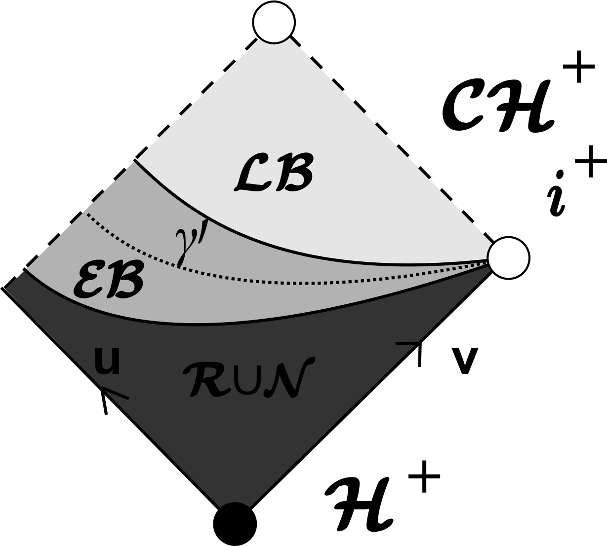
Figure 4: Penrose diagram of the space-time $\mathcal{M}=\mathcal{R}\cup\mathcal{N}\cup\mathcal{EB}\cup\mathcal{LB}$ with the inclusion of $\gamma^{\prime}$ .

5.2 Reduction to the proof of (3.5)

In this section, we want to highlight that the polynomial lower bound (3.5) for the derivative of $\phi$ transversally to the Cauchy horizon is enough to establish all the other claims of Theorem 3.3

The blow-up of the curvature follows directly from 3.5 as first highlighted in the pioneering work [26] : indeed we can consider

$$Ric(\Omega^{-2}\partial_{v},\Omega^{-2}\partial_{v})=\Omega^{-4}|\partial_{v}\phi|^{2}.$$

(3.5) then gives that :

$$\limsup_{v\rightarrow+\infty}Ric(\Omega^{-2}\partial_{v},\Omega^{-2}\partial_{v})(u,v)=+\infty,$$

using for instance the exponential lower bound for $\Omega^{-4}$ given by (5.18) in $\mathcal{V}$.

If $s>1$, we consider the continuous extension $\bar{M}$ and the future boundary null $\mathcal{CH}^{+}:=\{V\equiv 1,0\leq U\leq U_{0}\}$ mentioned in the statement of Theorem 3.2.

Notice that (5.11) proves in that case that $\partial_{v}\log(\Omega^{2}_{CH})(u,.)$ is integrable in $v$ hence $(u,V)$ is a regular coordinate system across the extension : in particular $\Omega^{2}_{CH}>0$ on $\mathcal{CH}^{+}$.

If $\mathcal{U}$ is a neighbourhood in $\bar{M}$ with compact closure -in particular with a finite range of $u$- of a point $p\in\mathcal{CH}^{+}$, and $\phi$ is a spherically symmetric function, its $W^{1,2}_{\mathcal{U}}$ norm can be expressed in $(u,V)$ and $(u,v)$ coordinates - as developed in [28]- as :

$$\|\phi\|^{2}_{W^{1,2}(\mathcal{U})}=\int_{\mathcal{U}}\left(|\partial_{V}\phi|^{2}+|\partial_{u}\phi|^{2}+|\phi|^{2}\right)dudV\sim\int_{\mathcal{U}}\left(\Omega^{-2}|\partial_{v}\phi|^{2}+\Omega^{2}(|\partial_{u}\phi|^{2}+|\phi|^{2})\right)dudv.$$ (5.19)

Since $\mathcal{U}$ is a neighbourhood of $p$, consider the smaller neighbourhood $\mathcal{U}^{\prime}:=\mathcal{U}\cap\mathcal{V}$.

Then, using the fact from (5.9) that $\partial_{v}\Omega^{2}\leq 0$ :

$$\|\phi\|^{2}_{W^{1,2}(\mathcal{U})}\gtrsim\int_{\mathcal{U}^{\prime}}\Omega^{-2}|\partial_{v}\phi|^{2}du^{\prime}dv^{\prime}.$$

We can then use (5.18) -valid in $\mathcal{U}^{\prime}$- with (3.5) to get

$$\|\phi\|_{W^{1,2}(\mathcal{U})}=+\infty,$$

i.e

$$\phi\notin W^{1,2}_{loc}.$$

Now we want to prove that the continuous extension to $\mathcal{CH}^{+}$ of Theorem 3.2 is not $C^{1}$.

We integrate (2.18) on $[v_{\gamma_{\mathcal{V}}}(u),v]$. Using that $\iota^{-1}\geq 0$ we get :

$$\iota^{-1}(u,v)\geq\iota^{-1}(u,v_{\gamma_{\mathcal{V}}}(u))+\int_{v_{\gamma_{\mathcal{V}}}(u)}^{v}\frac{4r}{\Omega^{2}}|\partial_{v}\phi|^{2}(u,v^{\prime})dv^{\prime}\gtrsim\int_{v_{\gamma_{\mathcal{V}}}(u)}^{v}\frac{|\partial_{v}\phi|^{2}(u^{\prime},v^{\prime})}{\Omega^{2}}dv^{\prime}.$$

Which means using the same argument as a few lines above that for all $u\leq u_{s}$ and when $v\rightarrow+\infty$ :

$$\iota^{-1}(u,v)=\frac{-4\lambda}{\Omega^{2}}\rightarrow+\infty.$$

And since $\iota^{-1}$ is unchanged for the coordinate system $(u,V)$ that is regular near the Cauchy horizon, i.e the system allowing for the continuous extension, it proves that the metric is not $C^{1}$ in the continuous extension of Theorem 3.2 for $s>1$.

5.3 Strategy to prove (3.5)

This time we split the space-time into two sub-regions only, namely the past and the future of the curve $\gamma^{\prime}:=\{r-r_{-}=v^{1-2s+\eta}\}$ for a well-chosen $0<\eta<2s-1$ small enough. This curve is similar to $\gamma$ introduced in section 4.6 -although it has a different power-, we will see that is is comparable near infinity to $\{u+v+h(v)=\Delta_{N}+\frac{2s-1-\eta}{2|K_{-}|}\log(v)\}$.

For the sake of comparison, as we will see $\gamma^{\prime}$ lies entirely in the early blue-shift transition region $\mathcal{EB}$ for $|u_{s}|$ large enough c.f Figure 4. The key use of this property is that $\kappa^{-1}$ and $\iota^{-1}$ are still bounded in $\mathcal{EB}$.

Since only the averaged - opposed to pointwise- lower bound of hypothesis 8 is available, we use a vector field method in the past of $\gamma^{\prime}$ with the Kodama vector field $T:=\kappa^{-1}\partial_{v}-\iota^{-1}\partial_{u}$ which is the geometric analog of the Killing vector field $\partial_{t}$ on Reisser-Nordström. However notice that unlike $\partial_{t}$ on Reisser-Nordström, $T$ is not a Killing vector field in general i.e $\Pi^{(T)}\neq 0$.

The study of $T$ is particularly relevant for two reasons : first there is no bulk term when we contract the deformation tensor $\Pi^{(T)}_{\mu\nu}:=\nabla_{(\mu}T_{\nu)}$ of $T$ with the stress-energy tensor $\mathbb{T}=\mathbb{T}_{EM}+\mathbb{T}_{KG}$ : $\Pi^{(T)}_{\mu\nu}\mathbb{T}^{\mu\nu}=0$.

Despite $\Pi^{(T)}\neq 0$, this is remarkable that we still get an exact conservation law , that we want to integrate.

Second, the good control of $\kappa^{-1}$ and $\iota^{-1}$ allows us to capture $|\partial_{v}\phi|$ appropriately. In particular on the event horizon $\mathcal{H}^{+}$, we see $\int_{\mathcal{H}^{+}}|\partial_{v}\phi|^{2}$ in gauge (3.1) which is exactly the term for which we have a lower bound that we want to propagate. The other terms, notably crossed terms, either enjoy a stronger decay or have a favourable sign.

In the future of $\gamma^{\prime}$, we simply use the propagation equation (2.27) and integrate along the $u$ characteristic taking advantage on the upper bound $\Omega^{2}\lesssim v^{-2s}$ on $\gamma^{\prime}$, using similar techniques to that of section 4.7. The key point is that the energy flux on $\gamma^{\prime}$ is controlled by the integral of $|\partial_{v}\phi|^{2}$ on $\gamma^{\prime}$. This is due to the fact that $\kappa^{-1}$ and $\iota^{-1}$ are bounded on $\gamma^{\prime}$ and also that $\gamma^{\prime}$ is rather symmetric in $u$ and $v$ apart from the term $v^{1-2s+\eta}$ which decays sufficiently . This symmetry avoids to consider terms of the form $\kappa^{-1}-\iota^{-1}$ which are bounded but do not a priori decay.

5.4 Up to the blue-shift region : the past of $\gamma^{\prime}$

We will use the same notations as in the stability part.

Moreover, for $v\geq v_{0}$, we introduce $\gamma^{\prime}_{v}:=\{(u^{\prime},v^{\prime})\in\gamma^{\prime},v^{\prime}\geq v\}$ and denote $u_{\gamma^{\prime}}(v)$ the unique $u$ such that $(u,v)\in\gamma^{\prime}$ and $\mathcal{H}^{+}_{v}:=\mathcal{H}^{+}\cap\{v^{\prime}\geq v\}$ . $n^{\prime}$ denotes the future directed unit normal of $\gamma^{\prime}$.

$vol$ is the standard volume form induced by the metric, and is written in $(u,v)$ coordinates as

$$vol=\Omega^{2}r^{2}\sin(\theta)dudvd\theta d\psi,$$

where $(\theta,\psi)$ are the standard coordinates on $\mathbb{S}^{2}$.

We also define the Kodama vector field $T:=\kappa^{-1}\partial_{v}-\iota^{-1}\partial_{u}$.

Proposition 5.1.

Under the hypothesis of Theorem 3.3 and for $v$ large enough, we have :

$$\int_{\gamma^{\prime}_{v}}\mathbb{T}(T,n^{\prime})vol(n^{\prime},.)\gtrsim v^{-p}.$$ (5.20)

Proof.

We state the following lemma, which is proven using elementary calculus only :

Lemma 5.2.

$$\mathbb{T}_{uu}=2|D_{u}\phi|^{2},$$ (5.21)

$$\mathbb{T}_{vv}=2|\partial_{v}\phi|^{2},$$ (5.22)

$$\mathbb{T}_{uv}=\frac{\Omega^{2}}{2}(m^{2}|\phi|^{2}+\frac{Q^{2}}{r^{4}}),$$ (5.23)

$$\Pi^{(T)}_{uu}=-2r|D_{u}\phi|^{2},$$ (5.24)

$$\Pi^{(T)}_{vv}=2r|\partial_{v}\phi|^{2},$$ (5.25)

$$\Pi^{(T)}_{uv}=\Pi^{(T)}_{\theta\theta}=\Pi^{(T)}_{\psi\psi}=0.$$ (5.26)

As a consequence, we see that $\Pi^{(T)}_{\mu\nu}\mathbb{T}^{\mu\nu}=0$.

Using the precedent lemma and applying the divergence theorem to the region delimited by $\mathcal{H}^{+}_{v}$, $\gamma^{\prime}_{v}$ and $\{v^{\prime}=v,u\leq u_{\gamma^{\prime}}(v)\}$ we get :

$$\int_{\gamma^{\prime}_{v}}\mathbb{T}(T,n^{\prime})vol(n^{\prime},.)\gtrsim\int_{\mathcal{H}^{+}_{v}}|\partial_{v}\phi|^{2}+4\lambda Q^{2}+4\lambda|\phi|^{2}+\int_{v^{\prime}=v,u\leq u_{\gamma^{\prime}}(v)}-\iota^{-1}|D_{u}\phi|^{2}-4\nu Q^{2}-4\nu|\phi|^{2}.$$ (5.27)

Now notice that $\lambda_{|\mathcal{H}^{+}}\geq 0$ as proved in 4.3.3, and $\nu\leq 0$ so all the terms in the right hand side are non-negative, except $-\iota^{-1}|D_{u}\phi|^{2}$. For this one, we write :

$$\int_{-\infty}^{u_{\gamma^{\prime}}(v)}\iota^{-1}(u^{\prime},v)|D_{u}\phi|^{2}(u^{\prime},v)du^{\prime}=\int_{-\infty}^{u_{\mathcal{R}}(v)}\iota^{-1}(u^{\prime},v)|D_{u}\phi|^{2}(u^{\prime},v)du^{\prime}+\int_{u_{\mathcal{R}}(v)}^{u_{\gamma^{\prime}}(v)}\iota^{-1}(u^{\prime},v)|D_{u}\phi|^{2}(u^{\prime},v)du^{\prime},$$

where $u_{\mathcal{R}}(v)$ is the unique $u$ such that $u+v+h(v)=-\Delta$ i.e $(u,v)$ belongs to the future boundary of $\mathcal{R}$.

The first term can be bounded using (5.2) :

$$|\int_{-\infty}^{u_{\mathcal{R}}(v)}\iota^{-1}(u^{\prime},v)|D_{u}\phi|^{2}(u^{\prime},v)du^{\prime}|\leq v^{-2s}|\int_{-\infty}^{u_{\mathcal{R}}(v)}4\lambda\Omega^{2}du^{\prime}|\lesssim v^{-2s}.$$

The second term using (5.3), (5.4) and $|u_{\gamma^{\prime}}(v)-u_{\mathcal{R}}(v)|\lesssim\log(v)$ :

$$|\int_{u_{\mathcal{R}}(v)}^{u_{\gamma^{\prime}}(v)}\iota^{-1}(u^{\prime},v)|D_{u}\phi|^{2}(u^{\prime},v)du^{\prime}|\lesssim v^{-2s}\log(v).$$

To sum up since $p<2s$ , it proves that $\int_{-\infty}^{u_{\gamma^{\prime}}(v)}\iota^{-1}(u^{\prime},v)|D_{u}\phi|^{2}(u^{\prime},v)du^{\prime}=o(v^{-p})$ hence, as claimed

$$\int_{\gamma^{\prime}_{v}}\mathbb{T}(T,n^{\prime})vol(n^{\prime},.)\gtrsim v^{-p}.$$

∎

Before moving to the next section, we will need to localise $\gamma^{\prime}$ with respect to the regions of the stability part to be able to use the stability estimates. This is done by the following lemma :

Lemma 5.3.

For $|u_{s}|$ large enough and $\eta>0$ small enough, $\gamma^{\prime}:=\{r-r_{-}=v^{1-2s+\eta}\}\subset\mathcal{EB}$.

Moreover we have :

$$\Omega^{2}(u_{\gamma^{\prime}}(v),v)\sim v^{1-2s+\eta}.$$ (5.28)

Proof.

Using (2.11), we can write :

$$(r-r_{-})(r-r_{+})=\frac{r^{2}\Omega^{2}}{4\iota\kappa}-2r(\varpi-M)+Q^{2}-e^{2}.$$

As a consequence of this equation and (5.4), (5.5), (5.6), (5.7) and (5.8) - all valid in $\mathcal{EB}$- we get that $|r-r_{-}|\lesssim v^{1-2s}$ on $\gamma_{2s-1}:=\{u+v+h(v)=\frac{2s-1}{2|K_{-}|}\log(v)\}$ so , since $\nu\leq 0$, $\gamma^{\prime}$ lies in the past of $\gamma_{2s-1}$ for $|u_{s}|$ large enough.

Using the same equation as above, we prove easily, still using (5.6) that on $\gamma_{N}=\{u+v+h(v)=\Delta_{N}\}$ and for $|u_{s}|$ large enough,

$$r-r_{-}\gtrsim 1.$$

Hence, because $\nu\leq 0$, it is clear that $\gamma^{\prime}$ lies in the future of $\gamma_{N}$, providing $2s-1-\eta>0$.

We conclude by noticing that the intersection of the future of $\gamma_{N}$ and the past of $\gamma_{2s-1}$ is included in $\mathcal{EB}$ for $|u_{s}|$ large enough.

The last claim (5.28) follows from using the above equality in the other way around : there exists $\tilde{C}>0$ such that :

$$\Omega^{2}=\tilde{C}|r-r_{-}|+O(v^{1-2s}),$$

where we used the remarks mentioned earlier in the proof.

∎

5.5 Towards the Cauchy horizon : the future of $\gamma^{\prime}$

We now want to propagate our lower bounds to the future of $\gamma^{\prime}$. To circumvent the lack of decay of $Q$ and $\varpi$ near the Cauchy horizon, we do not use a vector field method any more but a more classical integration along the constant $v$ characteristic, as it was done in the stability part.

Given the bound of Proposition 5.1, and since $p<\min\{2s,6s-3\}$, it will be enough to prove the following

Proposition 5.4.

The following lower bound for $\partial_{v}\phi$ near the Cauchy horizon is true :

$$\int_{\gamma^{\prime}_{v}}\mathbb{T}(T,n^{\prime})vol(n^{\prime},.)\lesssim\int_{v}^{+\infty}|\partial_{v}\phi|^{2}(u_{0},v^{\prime})dv^{\prime}+O(v^{-2s})+O(v^{3-6s+4\eta}).$$ (5.29)

Proof.

The proof will be decomposed into two steps : the first one is expressed by the following lemma : we identify $\mathbb{T}(T,n^{\prime})$ in terms of the scalar field using the decay of $\Omega^{2}$ and the control of $\kappa^{-1}$ :

Lemma 5.5.

The following estimate is true :

$$\int_{\gamma^{\prime}_{v}}\mathbb{T}(T,n^{\prime})vol(n^{\prime},.)\lesssim\int_{\gamma^{\prime}_{v}}|\partial_{v}\phi|^{2}(u_{\gamma^{\prime}}(v^{\prime}),v^{\prime})dv^{\prime}+O(v^{-2s}).$$ (5.30)

Proof.

We now write $\gamma^{\prime}=f^{-1}\{0\}$ where $f(u,v):=r(u,v)-r_{-}-v^{1-2s+\eta}$.

Using $g^{uv}=-2\Omega^{-2}$ , we can write for $0<\eta<2s-1$ :

$$df^{\#}=(\frac{\iota^{-1}}{2}-2\Omega^{-2}(2s-1-\eta)v^{-2s+\eta})\partial_{u}+\frac{\kappa^{-1}}{2}\partial_{v}.$$

Using the definition of $T$, we can derive :

$$\mathbb{T}(T,df^{\#})=\frac{\kappa^{-2}}{2}T_{vv}-\frac{\iota^{-2}}{2}T_{uu}-\frac{2(2s-1-\eta)\kappa^{-1}v^{-2s+\eta}}{\Omega^{2}}T_{uv}+\frac{2(2s-1-\eta)\iota^{-1}v^{-2s+\eta}}{\Omega^{2}}T_{uu}.$$

Now notice that the second and third term are negative if $2s-1-\eta>0$, which can be arranged for $\eta$ sufficiently small.

For the fourth, notice that on $\gamma^{\prime}$ :

$$\frac{\iota^{-1}v^{-2s+\eta}}{\Omega^{2}}T_{uu}=\frac{\iota^{-1}v^{-2s+\eta}}{\Omega^{2}}|D_{u}\phi|^{2}=O(v^{-2s-1}),$$

where we used (5.3), (5.28) and the fact that $\iota^{-1}$ is bounded on $\gamma^{\prime}$ by (5.4).

This gives, recalling that $T_{vv}=2|\partial_{v}\phi|^{2}$ and that $\kappa^{-2}$ is bounded on $\gamma^{\prime}$ by (5.5) :

$$\mathbb{T}(T,df^{\#})\lesssim|\partial_{v}\phi|^{2}+O(v^{-2s-1}).$$

Now, an elementary computation gives that there exists a bounded function $w$ such that :

$$\frac{1}{\sqrt{-g(df^{\#},df^{\#})}}vol(n^{\prime},.)=w(u,v)dvd\sigma_{\mathcal{S}^{2}}.$$

Noticing that $n^{\prime}=\frac{df^{\#}}{\sqrt{-g(df^{\#},df^{\#})}}$, we integrate $\mathbb{T}(T,n^{\prime})vol(n^{\prime},.)$ on $\gamma^{\prime}_{v}$ which gives the claimed lemma.

∎

Now we want to propagate point-wise using (2.27) and then integrate :

Lemma 5.6.

The following estimate is true for all $u\leq u_{s}$ :

$$\int_{\gamma^{\prime}_{v}}|\partial_{v}\phi|^{2}(u_{\gamma^{\prime}}(v^{\prime}),v^{\prime})dv^{\prime}\lesssim\int_{v}^{+\infty}|\partial_{v}\phi|^{2}(u,v^{\prime})dv^{\prime}+O(v^{3-6s+4\eta})+o(v^{-2s}).$$ (5.31)

Proof.

We now place ourselves in the future of $\gamma^{\prime}_{v}$, a region that lies in $\mathcal{EB}\cup\mathcal{LB}$.

We use (2.27) to get -after adding and subtracting a $\Omega^{2}e^{2}|\phi|$ term- :

$$|\partial_{u}(e^{iq_{0}\int_{u_{0}}^{u}A_{u}(u^{\prime},v)du^{\prime}}r\partial_{v}\phi)|\lesssim|\lambda||D_{u}\phi|+\Omega^{2}((m^{2}+e^{2})|\phi|+|Q^{2}-e^{2}||\phi|).$$

We now deal with each term separately. To the future of $\gamma^{\prime}_{v}$, included in $\mathcal{EB}\cup\mathcal{LB}$ we use (5.14) :

$$|\lambda|\lesssim\Omega^{2}+v^{-2s}.$$

We can also use in the same region the estimate (5.10) :

$$|D_{u}\phi|\lesssim|u|^{-s}+|u|^{-2s}b(u,v),$$

with $b(u,v):=|u|^{1-s}1_{\{s>1\}}+v^{1-s}1_{\{s<1\}}+\log(v)1_{\{s=1\}}$.

All put together, we get :

$$|\lambda||D_{u}\phi|(u,v)\lesssim\Omega^{2}|u|^{-s}+\Omega^{2}|u|^{-2s}b(u,v)+v^{-2s}|u|^{-s}+v^{-2s}|u|^{-2s}b(u,v).$$

We start by the third and fourth terms :

$$\int_{u_{\gamma^{\prime}}(v)}^{u}\left(v^{-2s}|u^{\prime}|^{-s}+v^{-2s}|u^{\prime}|^{-2s}b(u^{\prime},v)\right)du^{\prime}\lesssim v^{-2s}b(u,v).$$

The first and second terms are more complicated : at fixed $v$ we have to split between the part of $[u_{\gamma^{\prime}}(v),u]$ that is in $\mathcal{EB}$ : $[u_{\gamma^{\prime}}(v),u_{\gamma}(v)]$ and the one that is in $\mathcal{LB}$ : $[u_{\gamma}(v),u]$.

For $[u_{\gamma}(v),u]$, we use (5.16) :

$$\int_{u_{\gamma}(v)}^{u}\left(\Omega^{2}(u^{\prime},v)|u^{\prime}|^{-s}+\Omega^{2}(u^{\prime},v)|u^{\prime}|^{-2s}b(u^{\prime},v)\right)du^{\prime}\lesssim\int_{u_{\gamma}(v)}^{u}\left(v^{-2s}|u^{\prime}|^{-s}+v^{-2s}|u^{\prime}|^{-2s}b(u^{\prime},v)\right)du^{\prime}\lesssim v^{-2s}b(u,v).$$

On $[u_{\gamma^{\prime}}(v),u_{\gamma}(v)]$, we use (5.15) the strictly negative lower bound on $\partial_{u}\log(\Omega^{2})$ with Lemma 4.1 to get that :

$$\int_{u_{\gamma^{\prime}}(v)}^{u_{\gamma}(v)}\left(\Omega^{2}(u^{\prime},v)|u^{\prime}|^{-s}+\Omega^{2}(u^{\prime},v)|u^{\prime}|^{-2s}b(u^{\prime},v)\right)du^{\prime}\lesssim$$

$$\Omega^{2}(u_{\gamma^{\prime}}(v),v)|u_{\gamma^{\prime}}(v)|^{-s}+\Omega^{2}(u_{\gamma^{\prime}}(v),v)|u_{\gamma^{\prime}}(v)|^{-2s}b(u_{\gamma^{\prime}}(v),v)\lesssim v^{1-3s+\eta},$$

where we used in the last inequality that $v^{1-4s+\eta}b(u_{\gamma^{\prime}}(v),v)=o(v^{1-3s+\eta})$.

To estimate $\Omega^{2}((m^{2}+e^{2})|\phi|+|\phi||Q^{2}-e^{2}|)$, we use a similar technique, splitting $[u_{\gamma^{\prime}(v)},u]$ into $[u_{\gamma^{\prime}(v)},u_{\gamma_{\mathcal{V}}}(v)]\cup[u_{\gamma_{\mathcal{V}}}(v),u]$ where $\gamma_{\mathcal{V}}$ is defined in section 4.7 as the past boundary of $\mathcal{V}$.

Using estimates (5.12), (5.13) in $\mathcal{EB}$ together with calculus Lemma 4.1 and (5.15), we prove that -choosing $\epsilon_{0}=\frac{\eta}{2s-1-\eta}$- :

$$\int_{u_{\gamma^{\prime}(v)}}^{u_{\gamma_{\mathcal{V}}}(v)}\Omega^{2}(u^{\prime},v)((m^{2}+e^{2})|\phi|(u^{\prime},v)+|\phi|(u^{\prime},v)|Q^{2}-e^{2}|(u^{\prime},v))du^{\prime}\lesssim v^{1-3s+2\eta}.$$

Using (5.18) in $\mathcal{V}$ and $|\phi|+|Q-e|\lesssim b(u,v)$ gives a negligible contribution on $[u_{\gamma_{\mathcal{V}}}(v),u]$, because $\Omega^{2}$ is exponentially decreasing, which proves :

$$\int_{u_{\gamma^{\prime}(v)}}^{u}\Omega^{2}(u^{\prime},v)(|\phi|(u^{\prime},v)+|\phi|(u^{\prime},v)|Q^{2}-e^{2}|(u^{\prime},v))du^{\prime}\lesssim v^{1-3s+2\eta}.$$

Now we can use that $v^{-2s}b(u,v)=v^{-2s}|u|^{1-s}1_{\{s>1\}}+o(v^{1-3s+2\eta})$ if $\eta$ is small enough, combine all the estimates and integrate the first equation :

$$|e^{iq_{0}\int_{u_{0}}^{u}A_{u}(u^{\prime},v)du^{\prime}}r\partial_{v}\phi(u,v)-e^{iq_{0}\int_{u_{0}}^{u_{\gamma^{\prime}}(v)}A_{u}(u^{\prime},v)du^{\prime}}r\partial_{v}\phi(u_{\gamma^{\prime}}(v),v)|\lesssim v^{1-3s+2\eta}+v^{-2s}|u|^{1-s}1_{\{s>1\}}.$$

Making the difference, using upper and lower bounds for $r$ and squaring, we get :

$$|\partial_{v}\phi(u_{\gamma}(v),v)|^{2}\lesssim|\partial_{v}\phi(u,v)|^{2}+v^{2-6s+4\eta}+v^{-4s}|u|^{2-2s}1_{\{s>1\}}.$$

To conclude, it is enough to integrate the last estimate on $[v,+\infty]$ and noticing that $v^{1-4s}|u|^{2-2s}1_{\{s>1\}}=o(v^{-2s})$.

∎

The combination of the two lemmas proves the proposition after choosing $\eta$ small enough so that $p<6s-3-4\eta$.

∎

Appendix A A localisation of the apparent horizon $\mathcal{A}$

As a straightforward by-product of our framework, we prove that in a non-linear setting, the apparent horizon $\mathcal{A}:=\{\partial_{v}r=0\}$ cannot be too far or too close of the event horizon if the decay of the perturbation is upper and lower bounded.

Proposition A.1.

We keep the same hypothesis as for Theorem 3.2. $h$ is defined in equation (4.10).

We assume the following on the event horizon $\mathcal{H}^{+}$ :

Assumption 9.

$$C^{\prime}v^{-p-1}\leq\Omega_{H}^{2}(0,v)\int_{v}^{+\infty}\frac{|\partial_{v}\phi|^{2}(0,v^{\prime})}{\Omega_{H}^{2}(0,v^{\prime})}dv^{\prime},$$ (A.1)

$$|\partial_{v}\phi|(0,v^{\prime})\leq Cv^{-s},$$ (A.2)

for $2s-1\leq p$ and $C,C^{\prime}>0$.

Then there exists constants $C_{+}>0,C_{-}>0$ such that

$$\mathcal{A}\subset\{C_{-}v^{-p-1}\leq\Omega^{2}(u,v)\leq C_{+}v^{-2s}\}=\{-\tilde{C}-\frac{(p+1)}{2K_{+}}\log(v)\leq u+v+h(v)\leq-\frac{2s}{2K_{+}}\log(v)+\tilde{C}\}.$$

Remark 18.

Notice that because of the exponential growth of $\Omega^{2}_{H}$ established in section 4.3.3, assumption 9 is consistent with the conjectured tail of the $field$ as formulated in Price’s law of conjecture 1.6.

Remark 19.

Notice that if $\phi$ does not become constant near infinity on the event horizon, $\mathcal{A}$ is strictly to the future of $\mathcal{H}^{+}$. This is in particular true if one assumes a lower bound on $\partial_{v}\phi$ ,like (3.4) or (A.1). Coupled with (A.2), it proves that $\mathcal{A}$ must asymptotically approach time-like infinity.

Proof.

Using assumption (9) and (2.18) on the event horizon and recalling (4.4), we get :

$$v^{-p-1}\lesssim\lambda\lesssim v^{-2s}.$$

We can rewrite (2.15) in $(U,v)$ coordinates as :

$$\partial_{U}\lambda=\frac{-\Omega^{2}_{H}}{4}(2K-m^{2}r|\phi|^{2}).$$

Using (4.13), 4.23 and section 4.3.2, there exists $\delta>0$ small enough so that $K_{+}<2K-m^{2}r|\phi|^{2}<3K_{+}$ in $\mathcal{R}$.

We can then integrate between the event horizon and the apparent horizon for $U\in[0,U_{\mathcal{A}}]$ to get :

$$v^{-p-1}\lesssim\frac{4}{3K_{+}}\lambda(0,v)<\int_{0}^{U_{\mathcal{A}}}\Omega^{2}_{H}(U^{\prime},v)dU^{\prime}<\frac{4}{K_{+}}\lambda(0,v)\lesssim v^{-2s}.$$

Then we can use (4.16) to prove that :

$$\int_{0}^{U_{\mathcal{A}}}\Omega^{2}_{H}(U^{\prime},v)dU^{\prime}\sim\Omega^{2}(U_{\mathcal{A}},v).$$

Which gives the result.

∎

Appendix B Proof of Proposition 4.7 of section 4.5.1

We recall proposition 4.7 for convenience :

Proposition.

For small enough $\epsilon>0$, we have :

$$|\phi|+|\partial_{v}\phi|+|D_{u}\phi|\precsim 2^{N}v^{-s},$$ (B.1)

$$|A_{u}|\lesssim(N+1)\delta,$$ (B.2)

we also have :

$$|\log\Omega^{2}(u,v)-\log(-4(1-\frac{2M}{r}+\frac{e^{2}}{r^{2}}))|\precsim 4^{N}v^{1-2s},$$ (B.3)

$$0\leq 1-\kappa\precsim 5^{N}v^{-2s},$$ (B.4)

$$|1-\iota|\precsim 5^{N}v^{-p(s)},$$ (B.5)

$$|\partial_{u}\log(\Omega^{2})-2K|\precsim 5^{N}v^{-p(s)},$$ (B.6)

$$|\partial_{v}\log(\Omega^{2})-2K|\precsim 5^{N}v^{-2s},$$ (B.7)

$$|Q(u,v)-e|\lesssim 4^{N}v^{1-2s},$$ (B.8)

$$|\varpi(u,v)-M|\lesssim 4^{N}v^{1-2s}.$$ (B.9)

Proof.

We want to prove by induction on $k$ the following estimates on $\mathcal{N}_{k}:=\{u+v+h(v)=-\Delta+k\epsilon\}$ :

$$|\phi|+|\partial_{v}\phi|\leq D_{k}v^{-s},$$ (B.10)

$$|rD_{u}\phi|\leq D_{k}v^{-s},$$ (B.11)

$$|A_{u}|\lesssim A_{k},$$ (B.12)

$$|\log\Omega^{2}(u,v)|\leq C_{k},$$ (B.13)

$$\Omega^{2}\leq\frac{3}{2}\Omega^{2}_{max}(M,e),$$ (B.14)

$$0\leq 1-\kappa\lesssim E_{k}v^{-2s},$$ (B.15)

$$|1-\iota|\lesssim E_{k}v^{-p(s)},$$ (B.16)

$$|\partial_{u}\log(\Omega^{2})-2K|\lesssim E_{k}v^{-p(s)},$$ (B.17)

$$|\partial_{v}\log(\Omega^{2})-2K|\lesssim E_{k}v^{-2s},$$ (B.18)

$$|Q(u,v)-e|\lesssim D_{k}^{2}v^{1-2s},$$ (B.19)

$$|\varpi(u,v)-M|\lesssim D_{k}^{2}v^{1-2s},$$ (B.20)

with $D_{k}=2D_{k-1}$, $E_{k}=5E_{k-1}$ , $C_{k}=C_{k-1}+K_{max}\epsilon$, $A_{k}=(k+1)\delta$ and $K_{max}$ depending on $(e,M)$ only. $\Omega^{2}_{max}(M,e)$ is defined as :

$$\Omega^{2}_{max}(M,e):=4(\frac{M^{2}}{e^{2}}-1)=\sup_{r\in[r_{-}(M,e),r_{+}(M,e)]}4|1-\frac{2M}{r}+\frac{e^{2}}{r^{2}}|.$$

The initialization of the induction comes directly from the bounds of proposition (4.5), after choosing $D_{0}$, $E_{0}$ and $A_{0}$ consistently. Notice that $A_{0}\lesssim\delta$.

Supposing the bounds are established for $\mathcal{N}_{k-1}$, we bootstrap the following on $\mathcal{N}_{k}$ :

$$\Omega^{2}\leq 2\Omega^{2}_{max}(M,e),$$ (B.21)

$$|\phi|+|\partial_{v}\phi|\leq 2D_{k}v^{-s},$$ (B.22)

$$|1-\kappa|\leq 2E_{k}v^{-2s},$$ (B.23)

$$|1-\iota|\leq 2E_{k}v^{-2s}.$$ (B.24)

Notice that because $\nu<0$ and $\lambda_{|\mathcal{H}^{+}}\geq 0$, we have $r\leq r_{+}$ everywhere.

We first use (B.22) to prove (B.19) with (2.21) :

$$|Q(u,v)-e|\lesssim D_{k}^{2}v^{1-2s}.$$

Then we can use (B.21) with (B.24) to prove that $|\lambda|$ is bounded, (B.22), (B.23) to prove (B.20) with (2.24) for $|u_{s}|$ large enough :

$$|\varpi(u,v)-M|\lesssim D_{k}^{2}v^{1-2s}.$$

Notice that since $\Omega^{2}=-4\iota\kappa(1-\frac{2\varpi}{r}+\frac{Q^{2}}{r^{2}})$ -as seen in equation (2.11)- we have -forming the differences $\varpi-M$ and $Q^{2}-e^{2}$ and using (B.23), (B.24) for $|u_{s}|$ large enough :

$$0\leq-(1-\frac{2\varpi}{r}+\frac{Q^{2}}{r^{2}})=-(1-\frac{2M}{r}+\frac{e^{2}}{r^{2}})+O(D_{k}^{2}v^{1-2s}).$$

So -since $r_{-}$ cancels $(1-\frac{2M}{r}+\frac{e^{2}}{r^{2}})$- for all $\eta>0$, there exists $|u_{s}|(\eta)$ large enough so that $r_{-}-\eta<r$. For $\eta>0$ small enough, it can be easily shown that the supremum on $[r_{-}-\eta,r_{+}]$ is attained on $[r_{-},r_{+}]$ :

$$\Omega^{2}_{max}(M,e)=\sup_{r\in[r_{-}(M,e)-\eta,r_{+}(M,e)]}4|1-\frac{2M}{r}+\frac{e^{2}}{r^{2}}|.$$

Since $|\Omega^{2}|\leq 4|1-\frac{2M}{r}+\frac{e^{2}}{r^{2}}|+\tilde{C}v^{1-2s}$, bootstrap (B.21) is validated for $|u_{s}|$ large enough and proves (B.14).

Moreover, with the same technique using (2.11), (B.19), (B.20) and bootstrap (B.23), (B.24) we can prove (B.3), choosing $|u_{s}|$ large enough.

(B.19), (B.20) also prove that :

$$|2K(u,v)-2K_{M,e}(r(u,v))|\lesssim D_{k}^{2}v^{1-2s}.$$ (B.25)

Using the same argument as in the red-shift region and (B.24) we get -for $|u_{s}|$ large enough- :

$$|\partial_{v}(2K)|\lesssim\Omega^{2}\leq 2\Omega^{2}_{max}.$$ (B.26)

We denote $v_{i}=v_{i}(u)$ the unique $v$ such that $u+v+h(v)=\Delta_{i}$.

Notice that from (4.11) :

$$|h(v_{k-1})-h(v)|\lesssim v_{k-1}^{1-2s}|v-v_{k-1}|\approx|u|^{1-2s}|v-v_{k-1}|\approx v^{1-2s}|v-v_{k-1}|.$$

Hence , because $u+v+h(v)-\Delta_{k-1}\leq\epsilon$ is bounded :

$$v-v_{k-1}=\frac{u+v+h(v)-\Delta_{k-1}}{1+O(v^{1-2s})}=u+v+h(v)-\Delta_{k-1}+O(v^{1-2s})$$ (B.27)

We use (2.22) and (B.21) to get :

$$|\partial_{v}A_{u}|\lesssim 1.$$

Hence by induction, we get (B.12) with

$$|A_{u}|\leq A_{k-1}+\tilde{C}\epsilon\leq A_{k},$$

after choosing $\epsilon$ small enough compared to $\delta$.

Then we use (2.28) with (B.21), (B.22), (B.23) to get :

$$|rD_{u}\phi|\leq D_{k-1}|u|^{-s}+\tilde{C}D_{k}\epsilon v^{-s}.$$

Hence for $\epsilon$ small enough compared to $(C,e,M,q_{0},m)$, we get (B.11).

Using (2.27) and the same type of argument, we close bootstrap (B.22) and get (B.10) after integrating $\partial_{v}\phi$ on a $\epsilon$-small region.

We can then use bootstrap (B.21), (B.22) and (B.23) and notice that $|\partial_{u}\varpi|+|\partial_{u}Q^{2}|\lesssim D_{k}^{2}v^{-2s}$ to get from (2.26):

$$|\partial_{v}\log(\Omega^{2})-2K|\lesssim(E_{k}+D_{k}^{2})v^{-2s}\lesssim E_{k}v^{-2s}.$$ (B.28)

Then, because of the discussion above, $\frac{r_{-}(e,M)}{2}<r<r_{+}(e,M)$ therefore there exists $K_{max}=K_{max}(e,M)>0$ such that $|K|<K_{max}$.

Using (B.28) and the induction hypothesis, we prove (B.13) and get -choosing $|u_{s}|$ large enough- :

$$\Omega^{-2}\precsim e^{2K_{max}k\epsilon}.$$

Hence from (2.29) and (B.11) we get :

$$|\kappa-1|\leq E_{k-1}+\bar{C}D_{k}^{2}e^{2K_{max}k\epsilon}\epsilon=E_{k-1}+\bar{C}D_{0}^{2}e^{(\log(4)+2K_{max}\epsilon)k}\epsilon.$$

We proceed in two times : first with choose $\epsilon$ small enough so that $\log(4)+2K_{max}\epsilon\leq\log(5)$. We get :

$$|\kappa-1|\leq E_{k-1}+\bar{C}D_{k}^{2}e^{2K_{max}k\epsilon}\epsilon=E_{0}5^{k-1}+\bar{C}D_{0}^{2}5^{k}\epsilon.$$

Than we can choose $\epsilon$ even smaller so that bootstrap (B.23) is validated. (B.15), and (B.18) are proved simultaneously, using (2.26) for (B.18) similarly to what was done before.

Symmetrically in $v$ we use the same methods to close bootstrap (B.24) and to prove (B.16), (B.17).

The induction is then proved and the estimates of the proposition follow directly.

∎

Appendix C Proof of Lemma 4.3 of section 4.3.2

We recall Lemma 4.3 :

Lemma.

Under the same hypothesis than before and for $v_{0}^{\prime}>v_{0}$, if $U_{s}$ is sufficiently small there exists a constant $D>0$ depending on $C,e,M,q_{0},m^{2},s,v_{0}$ and $v_{0}^{\prime}$ such that

$$|D_{U}\phi(U,v_{0}^{\prime})|\leq D.$$ (C.1)

$$|\partial_{U}r(U,v_{0}^{\prime})|^{-1}\leq D.$$ (C.2)

Therefore, for any $\eta>0$ independent of any parameter, there exists a $v_{0}^{\prime}>0$ such that

$$|D_{U}\phi(U,v_{0}^{\prime})|\lesssim C,$$

and for all $v\geq v_{0}^{\prime}$ :

$$|2K(0,v)-2K_{+}|\leq\eta K_{+},$$

$$rm^{2}|\phi|^{2}(0,v)\leq\eta K_{+}.$$

Proof.

We will make the following bootstrap assumptions :

$$|\nu_{H}|\leq B_{1}$$ (C.3)

$$|Q|+|\phi|+|\partial_{v}\phi|\leq B_{2}$$ (C.4)

The set of points such that the bootstraps are valid is non empty because of the hypothesis of Theorem 3.2, for $B_{2}$ large enough with respect to $C$, $e$ and $v_{0}$ and $B_{1}>1$.

Notice that with our hypothesis $r(0,v)>0$ and since $[v_{0},v_{0}^{\prime}]$ is a compact, it is clear that $r(0,v)$ is upper and lower bounded by strictly positive constants that depend on $v_{0}$ and $v_{0}^{\prime}$.

If we integrate (C.3) for $U_{s}$ small enough compared to $B_{1}$, we see that the same conclusion holds true for $r(U,v)$ on the whole rectangle $[0,U_{s}]\times[v_{0},v_{0}^{\prime}]$ . We write $0<r_{min}<r<r_{max}$.

Then, notice that $\kappa(0,v)\equiv 1$ and the positive right hand side of (2.29) give that $0\leq\kappa\leq 1$ everywhere on the space-time namely $\Omega_{H}^{2}\leq-4\nu_{H}$.

Then we write (2.15) as

$$|\partial_{v}(\log(-r\nu_{H}))\leq\frac{1}{r}(1+\frac{Q^{2}}{r^{2}})+m^{2}r|\phi|^{2}\leq\frac{1}{r_{min}}+\frac{B_{2}^{2}}{r^{3}_{min}}+m^{2}r_{max}B_{2}^{2}.$$

We can then integrate in $v$ and use gauge (3.2) to get :

$$|\log(-\nu_{H})|\leq|\log(\frac{r_{max}}{r_{min}})|+(\frac{1}{r_{min}}+\frac{B_{2}^{2}}{r^{3}_{min}}+m^{2}r_{max}B_{2}^{2})(v_{0}^{\prime}-v_{0}).$$

This closes bootstrap (C.3) for $B_{1}$ large enough with respect to $B_{2}$, $v_{0}$, $v_{0}^{\prime}$ and the parameters and proves (C.2).

Now we want to bound $\lambda$ : to do so we write (2.15) as :

$$|\partial_{U}(r\lambda)|\leq-\nu_{H}(1+\frac{Q^{2}}{r^{2}}+m^{2}r^{2}|\phi|^{2})\leq B_{1}(1+\frac{B_{2}^{2}}{r^{2}_{min}}+m^{2}r^{2}_{max}B_{2}^{2}).$$

Now notice that on the compact $[v_{0},v_{0}^{\prime}]$, $|\lambda|(0,v)\leq\lambda_{max}$ where $\lambda_{max}$ depends on $v_{0}$, $v_{0}^{\prime}$ and the parameters.

Then we can integrate the previous equation and take $U_{s}$ small enough to get everywhere :

$$|\lambda|(U,v)\leq 2\lambda_{max}.$$

Now we write (2.28) as

$$|\partial_{v}(rD_{U}\phi)|\leq-\nu_{H}(m^{2}|\phi|+|\partial_{v}\phi|)\leq(m^{2}+1)B_{1}B_{2}.$$

Then we integrate and use assumption 5 and the bounds on $r$ to get :

$$|D_{U}\phi|\leq\frac{r_{max}}{r_{min}}C+\frac{(v_{0}^{\prime}-v_{0})(m^{2}+1)B_{1}B_{2}}{r_{min}}.$$ (C.5)

Now we use gauge (2.9) to integrate (2.22) :

$$|A_{U}|\leq\frac{2B_{1}B_{2}}{r_{min}^{2}}(v_{0}^{\prime}-v_{0}).$$

This, with bootstrap (C.4) and (C.5) gives :

$$|\partial_{U}\phi|\leq\frac{r_{max}}{r_{min}}C+\frac{(v_{0}^{\prime}-v_{0})B_{1}B_{2}}{r_{min}}[(m^{2}+1)+\frac{2q_{0}B_{2}}{r_{min}}].$$

It now suffices to integrate for $U_{s}$ small enough to close the $\phi$ part of bootstrap (C.4).

The $Q$ part of bootstrap (C.4) is validated when we integrate (2.20) using (C.5).

For the $\partial_{v}\phi$ part, we write (2.27) as :

$$|\partial_{U}(e^{iq_{0}\int_{U_{0}}^{U}A_{U}}r\partial_{v}\phi)|\leq|\lambda||D_{U}\phi|+|\nu_{H}|(rm^{2}|\phi|+\frac{q_{0}|Q||\phi|}{r})$$

Then, from all the bounds that precedes it is clear that we can integrate on $[0,U]$ and close the $\partial_{v}\phi$ part of bootstrap (C.4) if we chose $U_{s}$ small enough.

Notice that $B_{2}$ can be chosen to depend on $C$, $v_{0}$ and $e$ only. Hence $B_{1}$ can be chosen to depend on $v_{0}$, $v_{0}^{\prime}$ and the parameters only.

In the end both bootstraps are validated.

Notice that (C.5) gives actually (C.1) now that the bootstraps assumptions are proved.

From the last section 4.3.1, $2K(0,v)-2K_{+}\rightarrow 0$ when $v\rightarrow+\infty$ and from the hypothesis 4 and the boundedness of $r$ we know that $rm^{2}|\phi|^{2}\rightarrow 0$ when $v\rightarrow+\infty$. We can write $\max\{|2K(0,v)-2K_{+}|,rm^{2}|\phi|^{2}\}=K_{+}\epsilon(v)$ and $\epsilon(v)\rightarrow 0$ when $v\rightarrow+\infty$.

Therefore for all $\eta>0$ -independent of all the other constants- there exists $v_{0}^{\prime}$ -depending only on the parameters and $v_{0}$ such that for all $v^{\prime}\geq v_{0}^{\prime}$, $|\epsilon(v^{\prime})|\leq\eta$.

Therefore, combining with (C.1), the lemma is proven.

∎

References

• [1] Spyros Alexakis, Volker Schlue Non-existence of time periodic vacuum space-times. Journal of Differential Geometry, to appear. arXiv:1504.04592.
• [2] Piotr Bizoń, Arthur Wasserman On existence of mini-boson stars. Comm.Math.Phys.215:357-373 , 2000.
• [3] Lior Burko, Gaurav Khanna Universality of massive scalar field late-time tails in black-hole spacetimes. Phys.Rev. D70, 044018, 2004.
• [4] Otis Chodosh, Yakov Shlapentokh-Rothman, Time-periodic Einstein-Klein-Gordon bifurcations of Kerr. Preprint, 2016. arXiv:1510.08025.
• [5] Yvonne Choquet-Bruhat, Theoreme d’existence pour certains systemes d’equations aux derivees partielles non linaires. Acta Math. 88, 141–225, 1952.
• [6] Yvonne Choquet-Bruhat, Robert Geroch, Global Aspects of the Cauchy Problem in General Relativity. Comm. Math. Phys. 14, 329–335, 1969.
• [7] Demetrios Christodoulou, Violation of cosmic censorship in the gravitational collapse of a dust cloud. Comm. Math. Phys. 93, 171–195, 1984.
• [8] Demetrios Christodoulou, The Formation of Black Holes and Singularities in Spherically Symmetric Gravitational Collapse . Comm. Pure Appl. Math. 44, no. 3, 339–373, 1991.
• [9] Demetrios Christodoulou, Bounded Variation Solutions of the Spherically Symmetric Einstein-Scalar Field Equations . Comm. Pure Appl. Math. 46, 1131–1220, 1993.
• [10] Demetrios Christodoulou, The instability of naked singularities in the gravitational collapse of a scalar field. Ann. of Math. (2) 149, no. 1, 183–217, 1999.
• [11] Demetrios Christodoulou, The formation of black holes in general relativity. European Mathematical Society, 2009.
• [12] João L Costa, Pedro M Girão, José Natário, Jorge Drumond Silva, On the global uniqueness for the Einstein-Maxwell-scalar field system with a cosmological constant: I. Well posedness and breakdown criterion. Classical and Quantum Gravity, Volume 32, Number 1, 2014.
• [13] Mihalis Dafermos, Stability and instability of the Cauchy horizon for the spherically symmetric Einstein-Maxwell-scalar field equations. Ann. of Math. 158 , 875–928, 2003.
• [14] Mihalis Dafermos, The Interior of Charged Black Holes and the Problem of Uniqueness in General Relativity. Comm. Pure Appl. Math. 58, 0445–0504, 2005.
• [15] Mihalis Dafermos, Igor Rodnianski, Yakov Shlapentokh-Rothman, Decay for solutions to the wave equation on Kerr exterior spacetimes III : the full sub-extremal case $|a|<M$. Ann. of Math., 183, 787–913, 2016.
• [16] Mihalis Dafermos, Igor Rodnianski A proof of Price’s law for the collapse of a self-gravitating scalar field. Invent. math. 162, 381–457, 2005.
• [17] Mihalis Dafermos, Igor Rodnianski , Lectures on black holes and linear waves. 2008.
• [18] Mihalis Dafermos, Jonathan Luk, Stability of the Kerr Cauchy horizon . In preparation.
• [19] Anne Franzen Boundedness of massless scalar waves on Reissner-Nordström interior backgrounds. Commun. Math. Phys. 343: 601. doi:10.1007/s00220-015-2440-7, 2016.
• [20] Stephen Hawking, George Ellis, The large scale structure of space-time. Cambridge Monographs on Mathematical Physics, 1973.
• [21] Peter Hintz, Boundedness and decay of scalar waves at the Cauchy horizon of the Kerr spacetime. Commentarii Mathematici Helvetici, to appear. arXiv:1512.08003.
• [22] William Hiscock, Evolution of the interior of a charged black hole. Physics Letters A Volume 83, Issue 3, Pages 110–112, 1981.
• [23] Jonathan Kommemi, The Global Structure of Spherically Symmetric Charged Scalar Field Spacetimes. Commun. Math. Phys. 323: 35. doi:10.1007/s00220-013-1759-1, 2013.
• [24] Roman Konoplya, Alexander Zhidenko; A massive charged scalar field in the Kerr-Newman background I: quasi-normal modes, late-time tails and stability. Phys.Rev. D88 024054, 2013.
• [25] Philippe G. LeFloch, Yue Ma, The global nonlinear stability of Minkowski space for self-gravitating massive fields. The wave-Klein-Gordon model.Preprint, 2015. arXiv:1507.01143.
• [26] Jonathan Luk, Sung-Jin Oh, Strong Cosmic Censorship in Spherical Symmetry for two-ended Asymptotically Flat Initial Data I. The Interior of the Black Hole Region. Preprint, 2017.
• [27] Jonathan Luk, Sung-Jin Oh, Strong Cosmic Censorship in Spherical Symmetry for two-ended Asymptotically Flat Initial Data II. The Exterior of the Black Hole Region. Preprint, 2017.
• [28] Jonathan Luk, Sung-Jin Oh Proof of Linear Instability of the Reissner-Nordström Cauchy Horizon under Scalar Perturbations. Duke Math. J. Volume 166, Number 3, 437-493, 2017.
• [29] Jonathan Luk, Jan Sbierski Instability results for the wave equation in the interior of Kerr black holes. Journal of Functional Analysis, Volume 271, Issue 7, Pages 1948-1995, 2016.
• [30] Eric Poisson and Werner Israel Internal structure of black holes. Phys. Rev. D, 63:1663-1666, 1989.
• [31] Richard Price Nonspherical perturbations of relativistic gravitational collapse. I. Scalar and gravitational perturbations Phys. Rev. D (3) 5, 2419-2438, 1972.
• [32] Eric Poisson and Werner Israel Inner-horizon instability and mass inflation in black holes. Phys. Rev. Lett., 67(7):789-792, 1991.
• [33] Harvey Reall, Black Holes Lecture notes. Part III lecture notes, University of Cambridge, 2015.
• [34] Jan Sbierski, The C 0 -inextendibility of the Schwarzschild spacetime and the spacelike diameter in Lorentzian geometry. Preprint, 2016. arXiv:1507.00601.
• [35] Yakov Shlapentokh-Rothman, Exponentially growing finite energy solutions for the Klein-Gordon equation on sub-extremal Kerr spacetimes. Comm. Math. Phys. 309 no.3 859-891, 2014.
• [36] Michael Simpson, Roger Penrose Internal instability in a Reissner-Nordström black hole. Int J Theor Phys, 7: 183. doi:10.1007/BF00792069, 1973.
• [37] Terence Tao, Nonlinear dispersive equations : local and global analysis. CBMS, 2006.