Importance Sampled Stochastic Optimization for Variational Inference

Abstract

Variational inference approximates the posterior distribution of a probabilistic model with a parameterized density by maximizing a lower bound for the model evidence. Modern solutions fit a flexible approximation with stochastic gradient descent, using Monte Carlo approximation for the gradients. This enables variational inference for arbitrary differentiable probabilistic models, and consequently makes variational inference feasible for probabilistic programming languages. In this work we develop more efficient inference algorithms for the task by considering importance sampling estimates for the gradients. We show how the gradient with respect to the approximation parameters can often be evaluated efficiently without needing to re-compute gradients of the model itself, and then proceed to derive practical algorithms that use importance sampled estimates to speed up computation. We present importance sampled stochastic gradient descent that outperforms standard stochastic gradient descent by a clear margin for a range of models, and provide a justifiable variant of stochastic average gradients for variational inference.

1 INTRODUCTION

Variational inference considers parametric approximations for posterior densities of probabilistic models. Following Jordan et al. (1999) the classical variational approximation algorithms are based on coordinate descent algorithms for which individual steps of the algorithm are often carried out analytically. This limits the use of variational approximation to models with conjugate priors (or simple extensions of those) and restricts the family of potential approximating distributions based on analytic tractability.

Recent advances in variational approximation have lead to a phase transition; instead of closed-form updates, the approximation is nowadays often fit using generic gradient descent techniques instead – for a good overview see, e.g., Gal (2016). The key behind these advances is in using Monte Carlo approximation to estimate the gradient of the objective function that is an integral over the approximating distribution. This can be done in two alternative ways. The reparameterization estimate (Titsias and Lázaro-Gredilla, 2014; Kingma and Welling, 2014; Salimans and Knowles, 2013) allows expressing the gradient of the objective function using the gradients of the model itself, whereas the score function estimate (Ranganath et al., 2014) is based on gradients of the approximation. Given the new family of algorithms we can apply variational approximation for a considerably wider range of probabilistic models, enabling for example use of variational inference as the inference backend in probabilistic programming languages (Kucukelbir et al., 2017; Salvatier J, 2016; Tran et al., 2016).

The main research efforts in variational inference are nowadays geared towards making the approach applicable to a still wider family of models, by constructing even more flexible approximations (Rezende and Mohamed, 2015; Ranganath et al., 2016; Kingma et al., 2016) or by generalizing the gradient estimators (Ruiz et al., 2016; Naesseth et al., 2017). The question of how exactly the resulting optimization problem is solved has largely remained unattended to – practically all authors are satisfied with standard stochastic gradient descent (SGD) as the underlying optimizer, although some effort has been put into improving convergence by reducing the variance of the gradient estimate near the optimum (Roeder et al., 2017).

We turn our attention to the optimizer itself, looking into ways of speeding up the computation of gradient-based variational approximation. Practically all of the computational effort during learning goes into evaluating the gradient of the model (or the approximation if using the score-function estimate). Our contribution is in reducing the number of times we need to evaluate the gradient of the model during the optimization process, based on an importance sampling scheme specifically designed for optimization problems where the gradients are computed using Monte Carlo approximation.

The key observation is that the gradient of the objective function with respect to the parameters of the approximation consists of two parts. One part is the gradient of the model itself, evaluated at parameter values drawn from the approximation, whereas the other part is the gradient of the transformation used in the reparameterization estimate. We show that the gradient required for optimization can be computed for the newly updated approximation without re-computing the first part, which is computationally heavier. Instead, we can re-use existing computation by appropriately modifying and re-weighting the available terms.

We show how to formulate this idea in a justified manner, by constructing an importance sampling estimate for the gradient. Importance sampling is typically used for cases where one cannot sample from the distribution of interest but instead has to resort to sampling from a related proposal distribution. In our case we could sample from the distribution of interest – the current approximation – but choose not to, since by using an earlier approximation as a proposal we can avoid costly computation. The idea is conceptually similar to the way Gelman et al. (2017) reuses samples from previous iterations in expectation propagation.

Since the advances in our case are related to the computation of the gradient itself, the idea can readily be combined with several optimization algorithms. In this work, we derive practical algorithms extending standard SGD and stochastic average gradients (Schmidt et al., 2017). We demonstrate them in learning a variational approximation for several probabilistic models, showing how they improve the convergence speed in a model-independent manner.

In the following we first give a brief overview of the state-of-the-art in gradient-based variational approximation, covering both the gradient estimates and stochastic optimization algorithms in Section 2. We then proceed to describe the importance sampling estimate for the gradient in Section 3, followed by practical optimization algorithms outlined in Section 4. Empirical experiments and illustrations are provided in Section 5.

2 BACKGROUND

2.1 VARIATIONAL APPROXIMATION

Variational inference refers to approximating the posterior distribution $p(z|x)$ of a probabilistic model $p(x,z)$ using a distribution $q_{\lambda}(z)$ parameterized by $\lambda$. Usually this is achieved by maximizing a lower bound $\mathcal{L}(\lambda)$ for the evidence (also called the marginal likelihood) $p(x)$:

$$\mathcal{L}(\lambda)=\int q_{\lambda}(z)\log\frac{p(x,z)}{q_{\lambda}(z)}\ \delta z\leq p(x).$$ (1)

Traditionally, the problem has been made tractable by assuming a factorized mean-field approximation $q_{\lambda}(z)=\prod_{i}q_{\lambda_{i}}(z_{i})$ and models with conjugate priors, resulting in closed-form coordinate ascent algorithms specific for individual models – for a full derivation and examples, see, e.g., Blei et al. (2016).

In recent years several novel types of algorithms applicable for a wider range of models have been proposed (Titsias and Lázaro-Gredilla, 2014; Kingma and Welling, 2014; Salimans and Knowles, 2013; Ranganath et al., 2014), based on direct gradient-based optimization of the lower bound (1). The core idea behind these algorithms is in using Monte Carlo estimates for the loss and its gradient

$$\nabla_{\lambda}\mathcal{L}(\lambda)=\nabla_{\lambda}\mathbb{E}_{q_{\lambda}(z)}[\log p(x,z)-\log q_{\lambda}(z)].$$ (2)

Given such estimates, the inference problem can be solved by standard gradient descent algorithms. This enables inference for non-conjugate likelihoods and for complex models for which closed-form updates would be hard to derive, making variational inference a feasible inference strategy for probabilistic programming languages (Kucukelbir et al., 2017; Tran et al., 2016; Salvatier J, 2016). In the following, we briefly describe two alternative strategies of estimating the gradient. In Section 3 we will then show how the proposed importance sampling technique is applied for both cases.

2.1.1 REPARAMETERIZATION ESTIMATE

The reparameterization estimate for (1) (and consequently (2)) is based on representing the approximation $q_{\lambda}(z)$ using a differentiable transformation $z=f(\epsilon,\lambda)$ of an underlying standard distribution $\phi(\epsilon)$ that does not have any free parameters. The core idea of how this enables computing the gradient was developed simultaneously by Kingma and Welling (2014); Salimans and Knowles (2013) and Titsias and Lázaro-Gredilla (2014) with many of the mathematical details visible already in the early work by Opper and Archambeau (2009). Plugging the transformation $f(\cdot)$ into (1) gives

$$\mathcal{L}(\lambda)=\int\phi(\epsilon)\log\frac{p(x,f(\epsilon,\lambda))|\operatorname*{det}_{J_{f}}(\epsilon,\lambda)|}{\phi(\epsilon)}\ \delta\epsilon,$$

where the integral is over the standard distribution that does not depend on $z$, and $|\operatorname*{det}_{J_{f}}(\epsilon,\lambda)|$ is the absolute value of the determinant of the Jacobian of $f(\epsilon,\lambda)$. Consequently, it can be replaced by a stochastic approximation

$$\mathcal{L}(\lambda)=\frac{1}{M}\sum_{m=1}^{M}\log\frac{p(x,f(\epsilon_{m},\lambda))|\operatorname*{det}_{J_{f}}(\epsilon_{m},\lambda)|}{\phi(\epsilon_{m})},$$

where $\epsilon_{m}$ is drawn from $\phi(\epsilon)$. We can now easily compute the gradients using the chain rule, by first differentiating $\log p(x,f(\epsilon,\lambda))$ w.r.t $z$ and then $z=f(\epsilon,\lambda)$ w.r.t $\lambda$, resulting in

$$\nabla_{\lambda}\mathcal{L}(\lambda)\approx\frac{1}{M}\sum_{m=1}^{M}\left[\nabla_{z}\log p(x,z_{m})\nabla_{\lambda}f(\epsilon_{m},\lambda)+\nabla_{\lambda}|\text{det}_{J_{f}}(\epsilon_{m},\lambda)|\right].$$ (3)

The combination of the standard distribution $\phi(\epsilon)$ and the transformation $f(\epsilon,\lambda)$ defines the approximation family. For example, $\phi(\epsilon)=\mathcal{N}(0,I)$ and $f(\epsilon,\lambda=\{\mu,L\})=\mu+L\epsilon$ defines arbitrary Gaussian approximations (Opper and Archambeau, 2009; Titsias and Lázaro-Gredilla, 2014), where $L$ is the Cholesky factor of the covariance. To create richer approximations we can concatenate multiple transformations; Kucukelbir et al. (2017) combines the transformation above with a rich family of univariate transformations designed for different kinds of parameter constraints. For example, by using $f(\epsilon,\lambda=\{\mu,L\})=\operatorname*{Softplus}(\mu+L\epsilon)$ we can approximate parameters constrained for positive values. Alternatively, we can directly reparameterize other common distributions such as Gamma or Dirichlet – see Naesseth et al. (2017); Ruiz et al. (2016) for details.

2.1.2 SCORE FUNCTION ESTIMATE

An alternative estimate for (2) can be derived based on manipulation of the log-derivatives; the use of the estimate for simulation of models was originally presented by Kleijnen and Rubinstein (1995) and its use for variational approximation by Ranganath et al. (2014). The estimate for $\nabla_{\lambda}\mathcal{L}(\lambda)$ is provided by

$$\mathbb{E}_{q_{\lambda}(z)}[(\log p(x,z)-\log q_{\lambda}(z))\nabla_{\lambda}\log q_{\lambda}(z)],$$

which again leads into a straightforward Monte Carlo approximation of $\nabla_{\lambda}\mathcal{L}(\lambda)$ as

$$\frac{1}{M}\sum_{m=1}^{M}(\log p(x,z_{m})-\log q_{\lambda}(z_{m}))\nabla_{\lambda}\log q_{\lambda}(z_{m}),$$ (4)

where $z_{m}\sim{q_{\lambda}(z)}$. The notable property of this technique is that it does not require derivatives of the model (that is, $\log p(x,z)$) itself, but instead relies solely on derivatives of the approximation. This is both a pro and a con; the model does not need to be differentiable, but at the same time the estimate is not using the valuable information the model gradient provides. This is shown to result in considerably higher variance compared to the reparameterization estimate, often by orders of magnitude. Variance reduction techniques (Ranganath et al., 2014) help, but for differentiable models the reparameterization technique is typically considerably more efficient (Naesseth et al., 2017; Ruiz et al., 2016).

2.2 STOCHASTIC GRADIENT OPTIMIZATION

Given estimates for the gradient (2) computed with either method, the optimization problem is solved by standard gradient descent techniques. In practice all of the automatic variational inference papers have resorted to stochastic gradient descent (SGD) on mini-batches, adaptively tuning the step lengths with the state-of-the-art techniques.

In recent years several more advanced stochastic optimization algorithms have been proposed, such as stochastic average gradients (SAG) (Schmidt et al., 2017), stochastic variance reduced gradients (SVRG) (Johnson and Zhang, 2013), and SAGA that combines elements of both (Schatz et al., 2014). However, to our knowledge these techniques have not been successfully adapted for automatic variational inference. In Section 4.2 we will present a new variant of SAG that works also when the gradients are estimated as Monte Carlo approximations, and therefore briefly describe below the basic idea behind stochastic average gradients.

SAG performs gradient updates based on an estimate for the full batch gradient, obtained by summing up gradients stored for individual data points (or for mini-batches to save memory). Whenever a data point is seen again during the optimization the stored gradient for that point is replaced by the gradient evaluated at the current parameter values. The full gradient estimate hence consists of individual gradients estimated for different parameter values; the most recently computed gradients are accurate but the ones computed long time ago may correspond to vastly different parameter values. This introduces bias (Schatz et al., 2014), but especially towards the convergence the variance of the estimated full batch gradient is considerably smaller than that of the latest mini-batch, speeding up convergence.

3 METHOD

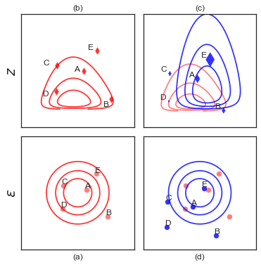
Figure 1: Importance sampling illustration for reparametrization gradients: A Monte Carlo estimate for the model evidence lower bound is obtained by drawing $M$ (here $5$) samples $z_{m}$ from the approximation $q(\lambda)$ depicted by the contours in top left panel. The reparameterization estimate does this by actually drawing the samples $\epsilon_{m}$ from a standard distribution depicted in the bottom left panel, transforming them to the parameter space with $f(\epsilon,\lambda)$. The importance sampling estimate for the evidence lower bound of another approximation $q(\lambda^{\prime})$ (top right) is obtained by keeping $z_{m}$ fixed and computing the $\epsilon_{m}^{\prime}=f^{-1}(z_{m},\lambda^{\prime})$ that would have been required as draws from the standard distribution (bottom right) to produce them. The estimate then re-weights the already computed log-likelihoods $\log p(x,z_{m})$ with $w_{m}=\frac{\phi(\epsilon_{m}^{\prime})}{\phi(\epsilon_{m})}$ to approximate the evidence lower bound; here sample E has higher probability under the new approximation, shown as larger diamond, and sample D has lower probability. The same basic procedure applies also for estimating the gradients instead of the evidence.

All gradient-based optimization algorithms follow the same basic pattern of computing a gradient for a mini-batch of samples and updating the parameters. The computational effort required goes almost solely into evaluating the gradient of the loss. To speed up the optimization, we next present a technique that allows computationally lighter evaluation of the gradient in scenarios where the gradient is computed using a Monte Carlo approximation. The presentation here is based on the reparameterization estimate (3) that benefits more off this treatment – as will become evident later – but for completeness we discuss also the score function estimate (4) in Section 3.2.

The Monte Carlo approximation for estimating the gradient depends on the data $x$ and a set of $M$ parameters $z_{m}$ drawn from the current approximation. As highlighted in (3), the actual computation factorizes into $\nabla_{z}p(x,z_{m})$ that depends only on $x$ and $z_{m}$ and into $\nabla_{\lambda}f(\epsilon,\lambda)$ and $\nabla_{\lambda}|\text{det}_{J_{f}}(\epsilon_{m},\lambda)|$ that depend only on $\epsilon_{m}$ and $\lambda$. The former part is typically considerably more computationally expensive. The observation that the slower part does not directly depend on the parameters hints that it should be possible to avoid re-computing the term even if the approximation changes, and this indeed is the case as explained next.

Assume we have already estimated the gradient at some parameters $\lambda$, implying that we have also evaluated $\nabla_{z}p(x,z_{m})$ for some set of $z_{m}$. The question now is how to estimate the gradient at parameters $\lambda^{\prime}=\lambda+\delta$ that are (typically only slightly) different. It turns out this can be done using the well-known concept of importance sampling originally designed for approximating expectations when we cannot directly draw samples from the density of interest. In our case, however, we could draw samples directly from the new approximation, but choose not to since the gradient can be estimated also using the old approximation as a proposal distribution. That is, we are using importance sampling for an unusual reason but can still use all the standard tools.

Typically, we use importance sampling to find the expectation of a function $f(z)$ over the target distribution $p(z)$ if we are able to draw samples only from a proposal distribution $q(z)$. The expectation of $f(z)$ over $p(z)$ can then be approximated by $$\mathbb{E}[f]=\int\frac{p(z)}{q(z)}f(z)q(z)\ \delta z=\frac{1}{M}\sum_{m=1}^{M}\frac{p(z_{m})}{q(z_{m})}f(z_{m}).$$ (5) The quantities $w_{m}={p(z_{m})}/{q(z_{m})}$ are the importance weights that correct the bias introduced by sampling from the wrong distribution $q(z)$ (Bishop, 2006). The weights $w_{m}$ are non-negative and tend to zero when $p(z)$ is completely mismatched to $q(z)$, and $w_{m}>1$ when the sample $z_{m}$ is more likely under the $p(z)$. The estimate above is unbiased, but has high – potentially infinite – variance when $q(z)$ and $p(z)$ are dissimilar. Next we show how importance sampling can be used for evaluating the reparameterization gradient (3).

To save computation we want to re-use the model gradients $\nabla_{z}\log p(x,z_{m})$ already available for certain values of $z_{m}$ and hence need to consider estimates that keep these values fixed. This means we need to find the $\epsilon_{m}^{\prime}$ under the new approximation $q_{\lambda^{\prime}}(z)$ that correspond to these values, by computing $\epsilon_{m}^{\prime}=f^{-1}(z_{m},\lambda^{\prime})$. Given these values we can evaluate the necessary quantities to compute both the importance weights and the other terms ($\nabla_{\lambda}f(\epsilon_{m}^{\prime},\lambda^{\prime})$ and $\nabla_{\lambda}|\text{det}_{J_{f}}(\epsilon_{m},\lambda)|$) required for evaluating the gradient itself.

The resulting importance sampling estimate for (3) is

$$\nabla^{i}_{\lambda}\mathcal{L}(\lambda)\approx\frac{1}{M}\sum_{m=1}^{M}\left[{\nabla_{z}\log p(x,z_{m})}\nabla_{\lambda}f(\epsilon^{\prime}_{m},\lambda^{\prime})+\nabla_{\lambda}|\text{det}_{J_{f}}(\epsilon^{\prime}_{m},\lambda^{\prime})|\right]\times w_{m},$$ (6)

where the $i$ in $\nabla^{i}_{\lambda}\mathcal{L}(\lambda)$ refers to the importance-sampled estimate of the gradient. The computationally expensive part of the gradient $\nabla_{z}\log p(x,z_{m})$ is already available and need not be computed. The rest of the terms are efficient to evaluate, and hence the whole gradient estimate is obtained in a fraction of a time compared to computing it from scratch. The importance weights are provided by

$$w_{m}=\frac{\phi(\epsilon_{m}^{\prime})}{\phi(\epsilon_{m})}$$ (7)

and hence only require evaluating densities of the standard distribution underlying the approximation. The above description is summarized in Algorithm 1 and illustrated graphically in Figure 1.

It is also worth noting that if $f(\cdot)$ is constructed as a series of transformations, for example as element-wise transformations of reparameterized normal distribution as done by (Kucukelbir et al., 2017), then parts of the term $\nabla_{\lambda}|\text{det}_{J_{f}}(\epsilon^{\prime}_{m},\lambda^{\prime})|$ can (and naturally should) also be re-used. This is, however, of secondary importance compared to the computational saving of re-using $\nabla_{z}\log p(x,z_{m})$.

A practical challenge with importance sampling is that for high-dimensional densities the weights $w_{m}$ easily tend to zero. Variational approximation is, however, often conducted for approximations that factorize over the parameters of the approximation as $q(\lambda)=\prod_{s}q(\lambda_{S_{s}})$, where $\{S_{s}\}$ is a partitioning of the parameter vector. The importance sampling estimate can – and should – be done for each factor separately, since the gradient $\nabla_{z}\log p(x,z_{m})$ can be computed for each approximation factor independently even if $\log p(x,z_{m})$ itself does not factorize. We show in Section 5.1 that the technique helps at least until factors consisting of roughly ten parameters.

input : Samples $z_{m}$ and $\epsilon_{m}$, gradient $\nabla_{z}p(x,z_{m})$, transformation $f()$, current approximation $\lambda^{\prime}$

output : Importance sampled gradients $\nabla_{\lambda}^{i}\mathcal{L}(\lambda)$

$\epsilon_{m}^{\prime}\leftarrow f^{-1}(z_{m},\lambda^{\prime})$

$w_{m}\leftarrow\frac{\phi(\epsilon^{\prime}_{m})}{\phi(\epsilon_{m})}$

Calculate $\nabla^{i}_{\lambda}\mathcal{L}(\lambda)$ using (6)

Algorithm 1 Importance sampled gradients

3.1 REPARAMETERIZATION GRADIENT EXAMPLE

To further clarify the derivation above, we next illustrate the procedure for the common scenario of Gaussian reparameterization combining $\phi(\epsilon)=\mathcal{N}(0,I)$ with $z=\mu+L\epsilon$, denoting $\lambda=\{\mu,L\}$. Given a set of $z_{m}$ drawn from $q(\lambda)$ we want to estimate the gradient evaluated at $\lambda^{\prime}$ using (6).

First we compute $\epsilon_{m}^{\prime}=f^{-1}(z_{m},\lambda^{\prime})=L^{-1}(z_{m}-\mu)$ and evaluate $\phi(\epsilon_{m}^{\prime})$ under the standard normal distribution. The weight $w_{m}$ can then readily be evaluated using (7), computing $\phi(\epsilon_{m})$ as well if it has not already been evaluated because of being used for another importance sampling estimate.

To compute the gradient (6) we need to re-compute $\nabla_{\lambda}f(\epsilon_{m}^{\prime},\lambda^{\prime})$ and $\nabla_{\lambda}|\text{det}_{J_{f}}(\epsilon^{\prime}_{m},\lambda^{\prime})|$. For $\mu$ these terms are simply identity and zero, whereas for $L$ we get $z_{m}$ and $\nabla_{L}\log|L^{\prime}|\equiv\Delta_{L^{\prime}}$. The exact form of $\Delta_{L^{\prime}}$ depends on the assumptions made for $L$; see Titsias and Lázaro-Gredilla (2014) for details. The final importance sampled estimate for the gradient is then

$$\nabla_{\mu}^{i}\mathcal{L}(\mu^{\prime},L^{\prime}) \approx\frac{1}{M}\sum_{m=1}^{M}w_{m}\nabla_{z}\log p(x,z_{m})$$

$$\nabla_{L}^{i}\mathcal{L}(\mu^{\prime},L^{\prime}) \approx\frac{1}{M}\sum_{m=1}^{M}w_{m}\left[\nabla_{z}\log p(x,z_{m})\epsilon^{\prime}_{m}+\Delta_{L^{\prime}}\right].$$

An important observation here is that the importance sampling procedure does not merely re-weight the terms $\nabla_{z}\log p(x,z_{m})$, but in addition the transformation that converts them into the $\lambda$ space changes because of the new values of $\epsilon_{m}^{\prime}$. These values depend on the approximation parameters in a non-linear fashion and hence the gradient itself is a non-linear transformation of the gradient evaluated at $\lambda$ (for a graphical illustration, see Figure 2). This is crucially important for development of the practical optimization algorithms in Section 4; if the transformation was linear then the importance sampling estimate would not necessarily provide improvement over careful adaptation of element-wise learning rates.

3.2 SCORE FUNCTION ESTIMATE

Above we discussed the importance sampling estimate from the perspective of the reparameterization estimate. For completeness we also show how it can be applied for the score function estimate, and discuss why it is less useful there.

The Monte Carlo approximation for the score function (4) is obtained directly by drawing samples from the approximation $q(\lambda)$. To approximate the gradient for $q(\lambda^{\prime})$ we merely use the standard importance sampling equation (5) to obtain the approximation

$$\frac{1}{M}\sum_{m=1}^{M}w_{m}\left[\log p(x,z_{m})-\log q_{\lambda}(z_{m})\right]\nabla_{\lambda}\log q_{\lambda}(z_{m}),$$

where $w_{m}=\frac{q(z|\lambda^{\prime})}{q(z|\lambda)}$. This is still an unbiased estimate, but the computational saving is typically smaller than in the reparameterization case. We do not need to evaluate $\log p(x,z_{m})$ since the samples $z_{m}$ are kept constant, but all other terms need to be computed again and evaluating the gradient of the approximation is not cheap. This estimate is only useful when the evaluation of the log probability utterly dominates the total computation.

4 ALGORITHMS

In the following we describe example optimization algorithms based on the importance sampling idea. The details are provided for a straightforward variant of SGD and for a generalization of stochastic average gradients, but other related algorithms could be instantiated as well.

4.1 IMPORTANCE SAMPLED SGD

input : data $X$, model $p(x,z)$, the variational approximation $q_{\lambda}(z)$, threshold $t$

output : variational parameters $\lambda^{*}$

while $\mathcal{L}(\lambda)$ has not converged do

       if $\text{random\_uniform}<t$ then

             Retrieve last stored $z_{m}$, $\epsilon_{m}$ and $\nabla_{z}\log p(x,z_{m})$

             Update $\nabla_{\lambda}\mathcal{L}$ using Algorithm (1)

            

      else

             Draw mini-batch $x$ from $X$

             $\epsilon_{m}\sim\phi(\epsilon)$

             $z_{m}\leftarrow f(\epsilon_{m},\lambda)$

             Update $\nabla_{\lambda}\mathcal{L}$ using Equation (3)

             Store $z_{m}$, $\epsilon_{m}$ and $\nabla_{z}\log p(x,z_{m})$

            

       end if

      Update $\lambda\leftarrow\lambda+\rho\nabla_{\lambda}\mathcal{L}(\lambda)$

      

end while

Algorithm 2 Importance sampled SGD

Stochastic gradient descent estimates the gradient based on a mini-batch and then takes a step along the gradient direction, typically using adaptive learning rates such as those by Kingma and Ba (2015); Duchi et al. (2010).

The importance sampled SGD (I-SGD; Algorithm 2) follows otherwise the same pattern, but for each mini-batch we conduct several gradient steps instead of just one. For the first one we evaluate the gradient directly using (2). After updating the approximation we apply Algorithm 1 to obtain an importance-sampled estimate for the gradient evaluated at the new parameter values, and proceed to take another gradient step using that estimate. For each step we use a proper estimate for the mini-batch gradient that can, after the first evaluation, be computed in a fraction of a time. After taking a few steps we then proceed to analyze a new mini-batch, again needing to compute the gradient from scratch since now $x$ has changed.

After passing through the whole data we have evaluated $\log p(x,z)$ and its gradient once for every data point, just as in standard SGD. However, we have taken considerably more gradient steps, possibly by a factor of ten. Alternatively, we can think of it as performing more updates given a constant number of model gradient evaluations.

A practical detail concerns the choice of how many steps to take for each mini-batch. This choice is governed by two aspects. On one hand we should not use the importance sampled estimate if the approximation has changed too much since computing the $\nabla_{z}\log p(x,z_{m})$ terms, recognized typically as $w_{m}$ tending to zero. On the other hand, we should not take too many steps even if the approximation does not change dramatically, since the gradient is still based on just a single mini-batch.

The empirical experiments in this paper are run with a simple heuristic that randomly determines whether to take another step with the current mini-batch or to proceed to the next one. This introduces a single tuning parameter $t$ that controls the expected number of steps per mini-batch. The algorithm is robust for this choice; we obtain practical speedups with values ranging from $t=0.5$ to $t=0.9$. Finally, importance-sampling could in principle result in very large gradients if $w_{m}\gg 1$ for some $m$; we never encountered this in practice, but a safe choice is to proceed to the next batch if that happens.

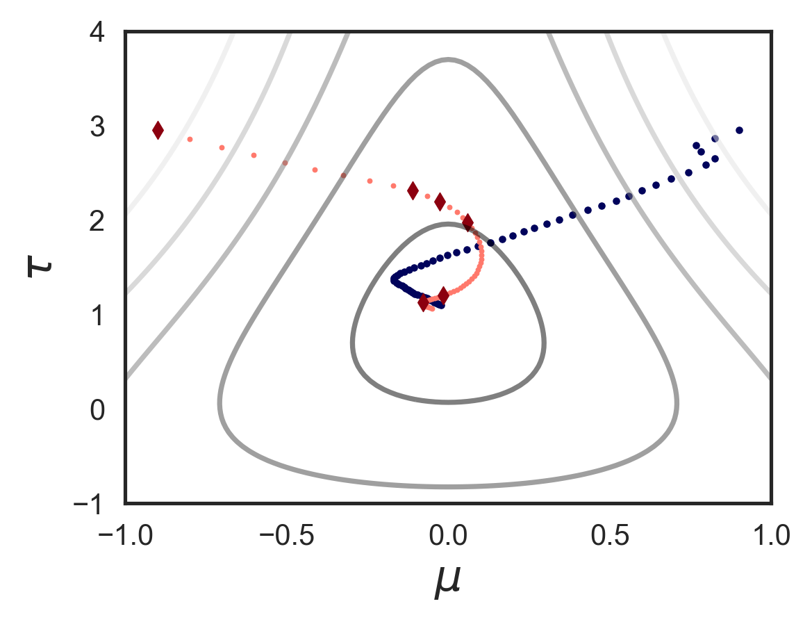
Figure 2: Illustration of I-SGD. I-SGD learns to approximate the posterior of a univariate normal distribution (parameterized by mean and precision) by computing the gradient of the evidence lower bound only a few times from scratch, indicated by red diamonds. Between these operations it performs multiple gradient steps (small red dots) using importance sampling estimates for the gradient that can be computed in a fraction of a time, while still following a non-linear trajectory between the red diamonds. For comparison, standard SGD, needs to estimate the full gradient for every step (blue dots).

For a practical illustration of the algorithm, see Figure 2 that approximates the posterior over the mean and precision of a normal model. Here $t=0.9$ and hence we take on average $9$ importance-sampled gradient steps for each mini-batch. The I-SGD algorithm reaches the optimum in roughly as many steps as conventional SGD but achieves it almost ten times faster.

input : data $X$, model $p(x,z)$, the variational approximation $q_{\lambda}(z)$, batches $B$

output : variational parameters $\lambda^{*}$

while $\mathcal{L}(\lambda)$ has not converged do

       foreach mini-batch $x_{b}$ in $X$ do

             $\epsilon^{b}_{m}\sim\phi(\epsilon)$

             $z^{b}_{m}\leftarrow f(\epsilon_{m},\lambda)$

             Calculate $\nabla^{b}_{\lambda}\mathcal{L}$ using Equation (3)

             Store $z^{b}_{m}$, $\epsilon^{b}_{m}$ and $\nabla^{b}_{z}\log p(x_{b},z_{m})$

             foreach mini-batch $x_{c}$ in $X\backslash\{x_{b}\}$ do

                   Retrieve $z^{c}_{m}$, $\epsilon^{c}_{m}$ and $\nabla^{c}_{z}\log p(x_{c},z_{m})$

                   Update $\nabla^{c}_{\lambda}\mathcal{L}$ using Algorithm (1)

                  

             end foreach

            $\nabla_{\lambda}\mathcal{L}\leftarrow\sum_{n=1}^{B}\nabla_{\lambda}^{n}\mathcal{L}$

             Update $\lambda\leftarrow\lambda+\rho\nabla_{\lambda}\mathcal{L}(\lambda)$

            

       end foreach

      

end while

Algorithm 3 Importance sampled SAG

4.2 IMPORTANCE SAMPLED SAG

Stochastic average gradients (Schmidt et al., 2017) stores the batch gradient and iteratively updates it for the samples in a given mini-batch. In the following we derive a variant of SAG (Algorithm 3) that uses importance sampling to both re-weight and update the gradients for the historical mini-batches using (6), helping to detect and avoid using stale gradients whose parameter values have changed so much since computing them.

When visiting a new mini-batch we compute the gradient using (3). For all previously visited mini-batches we compute the importance weights and modify the gradient according to (6). The whole gradient is formed by summing up the terms for all mini-batches. It is important to note that the importance sampling changes the weight of the gradient, decreasing it towards zero for the mini-batches evaluated under clearly different parameter settings, and transforms the gradient to better match one that would have been calculated under the current approximation.

This algorithm provides a justified version of SAG for automatic variational inference. The computational cost is higher than for standard SAG since we need to evaluate the importance weights and compute the terms related to the gradient of the transformation for all past mini-batches. There is, however, no additional memory overhead and the amount of evaluations for the gradient of the model itself is the same. This overhead for importance sampling the gradients for other batches is not negligible, but usually still small enough that the resulting algorithm outperforms a naive implementation of SAG because of vastly more accurate gradient estimates, as shown in Section 5.3. In case updating the past gradients becomes too costly, a simple remedy is to use only the latest $K$ mini-batches for some reasonable choice of $K$.

5 EXPERIMENTS

In this section we first demonstrate how the behavior of importance sampling depends on the dimensionality of the approximation. We then empirically compared both I-SGD and I-SAG for real variational inference tasks on a range of alternative models and settings.

5.1 DIMENSIONALITY OF THE APPROXIMATION

Figure 3 studies importance weights of approximations factorized at different granularities on a 100-dimensional diagonal multivariate Gaussian. An important observation is that even if importance sampling itself fails for factors of high dimensionality, the I-SGD algorithm degrades gracefully. For low-dimensional factors, up to at least 5-10 dimensions, we can safely take 5-10 steps with each mini-batch while still having accurate gradient estimates. When the dimensionality of individual factors reaches around $25$ the weights tend to zero already after a single gradient step, but the algorithm does not break down. It merely needs to proceed immediately to the next step, reverting back to standard SGD.

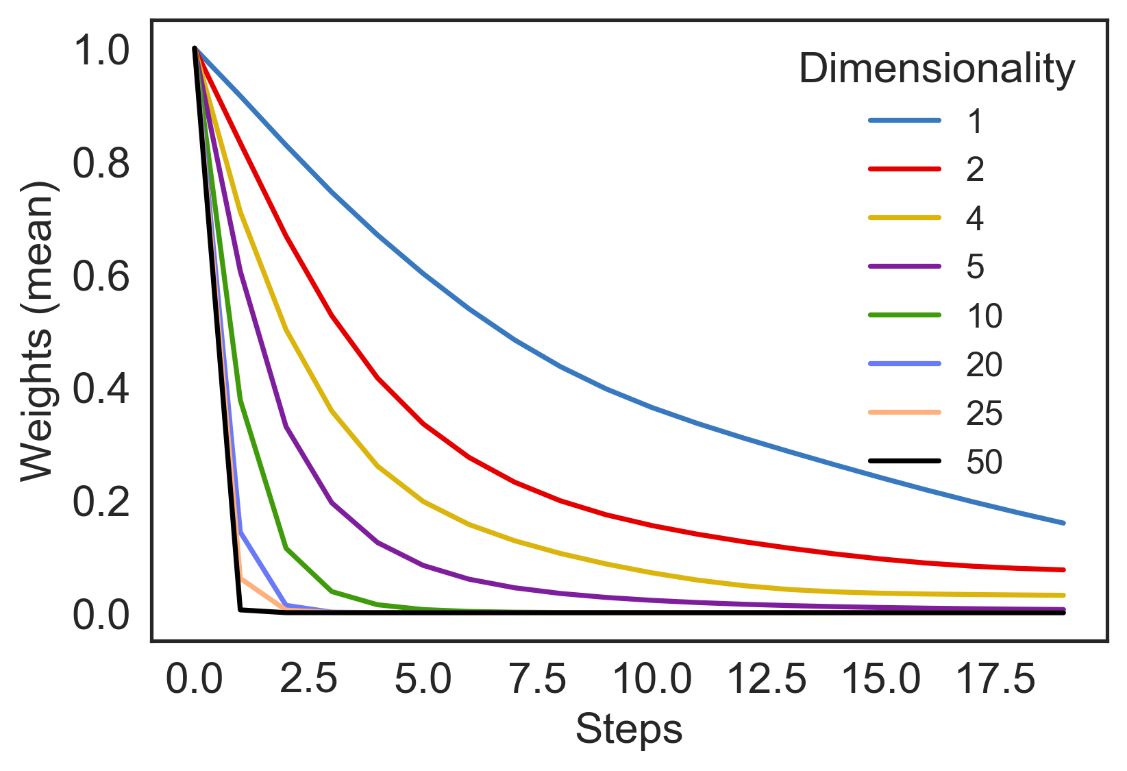
Figure 3: Importance sampling and dimensionality: Illustration of the behavior of the importance sampling weights during optimization for approximations of varying dimensionality. The approximation $q(\theta|\lambda)$ is over a 100-dimensional space and is factorized as $\prod_{i}q(\theta_{S_{i}}|\lambda_{i})$ so that the color of the line indicates the size of each term; for example, the purple line corresponds to factorized approximation with 20 terms of 5 variables. For fully factorized approximation (blue line) and still for factors of 5-10 dimensions the weights decay slowly and it pays off to take a few gradient steps before re-calculating the gradient. For factors of 25 (yellow line) or more dimensions the weights drop to zero practically immediately. The I-SGD algorithm still works, but does not give any speed advantage.

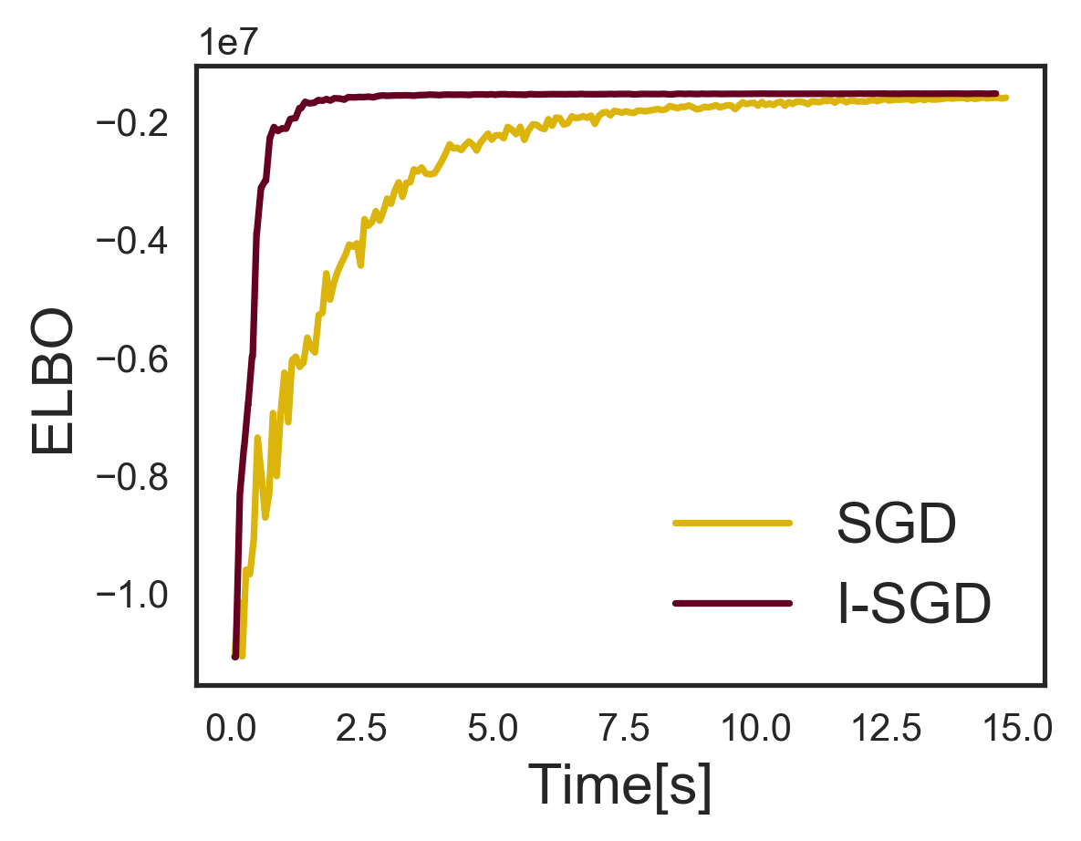
(a)

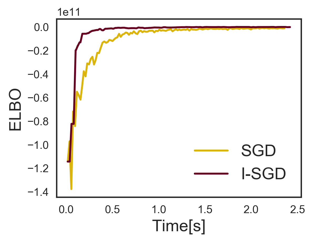
(b)

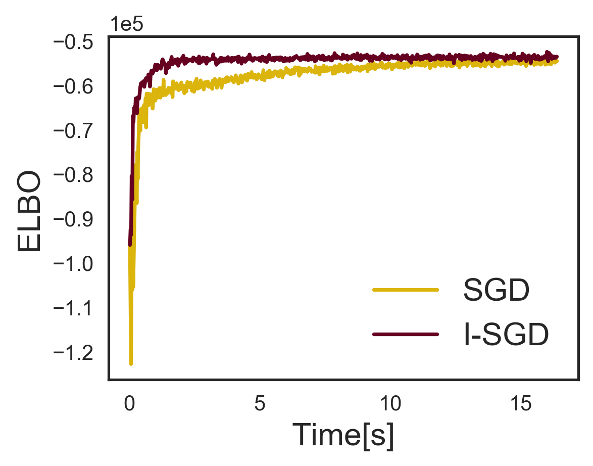
(c)

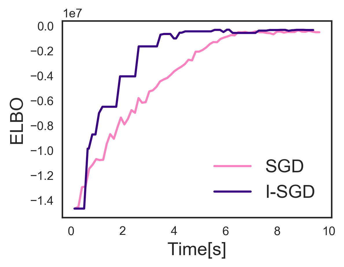
(d)

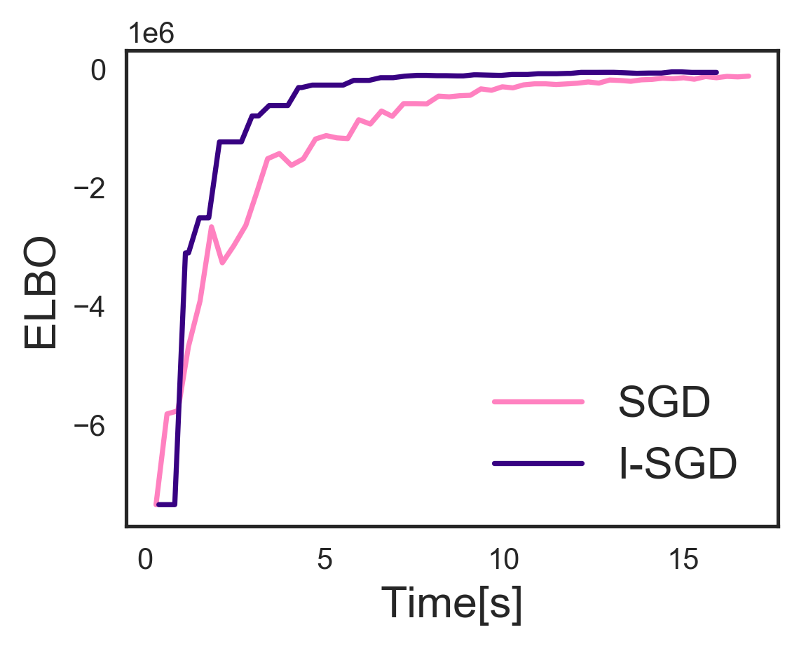
(e)

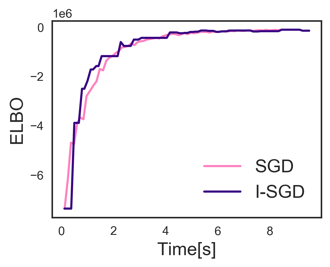
(f)

Figure 4: Performance of I-SGD on different models and gradient estimates: We evaluate the performance of I-SGD for reparameterization gradients in the top row and for score function gradients on the bottom row. For the reparameterization gradients our algorithm converges an order of magnitude faster than SGD for all three models. The computational savings in score function gradient is directly proportional to the complexity of the model’s log-probability and the simplicity of the variational approximation; in (d) evaluating the model dominates the total cost whereas in (f) the advantage of I-SGD is lost because less computation is saved. For description of the models refer to Section 5.2.

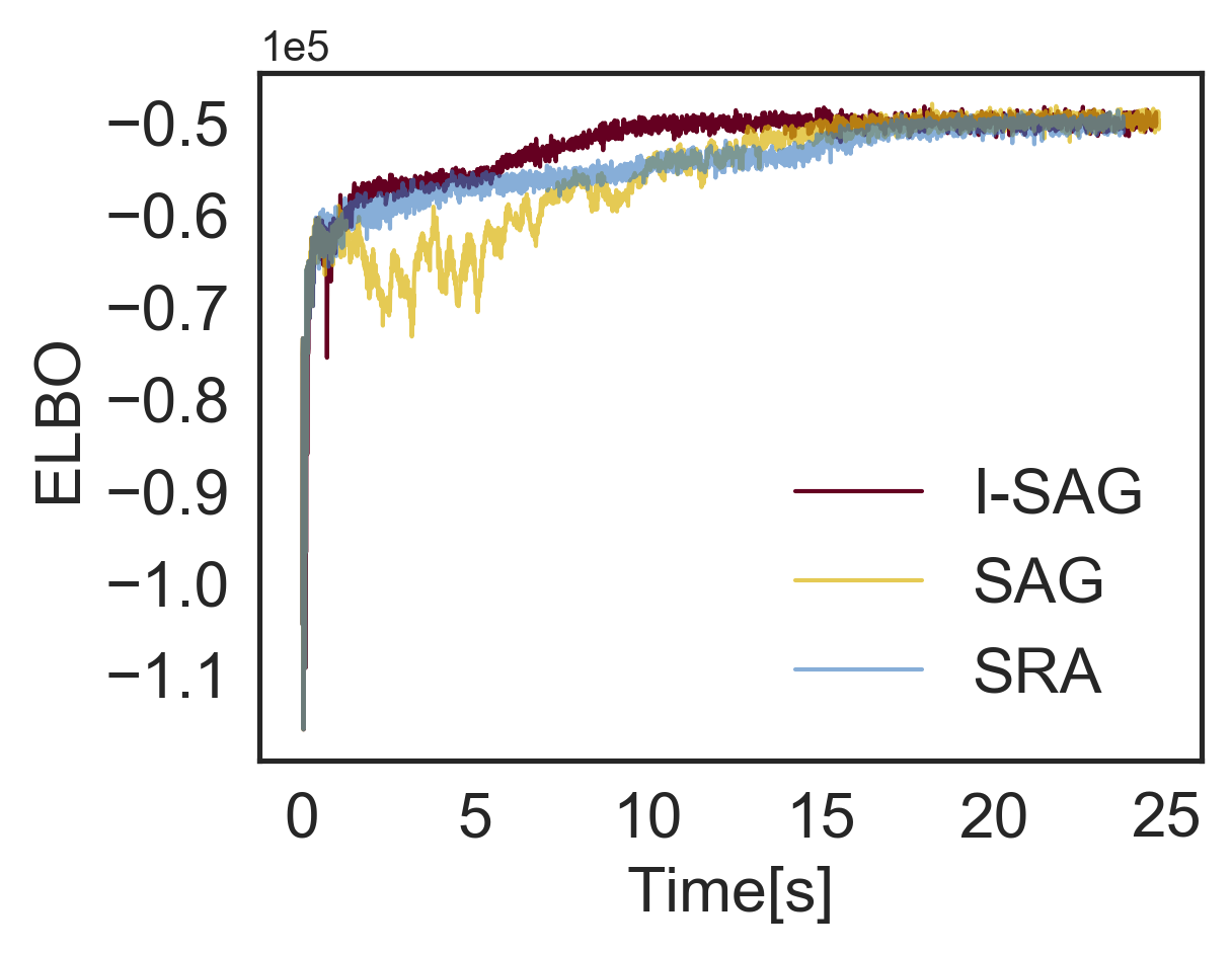
Figure 5: Importance Sampled Stochastic Average Gradient: Standard SAG algorithm (yellow line) performs poorly when using Monte Carlo approximation for the gradients. This can be in part overcome by considering a running average (SRA) of the mini-batch gradients instead (blue line, with $\alpha=0.9$ as the decay factor), letting the algorithm ignore stale gradients. The I-SAG algorithm (red line) outperforms both because it down-weights mini-batch gradients evaluated earlier in a more justified manner and because it also transforms the historical gradients to match the current approximation instead of using them directly.

5.2 IMPORTANCE SAMPLED SGD

We show in Figure 4 how I-SGD consistently bests SGD for a variety of different models, especially for the reparameterization estimate. For these experiments we use fully factorized mean-field approximation,

We first apply the reparameterization estimate for three probabilistic models: (a) a diagonal multivariate Gaussian with a standard normal prior on the mean and Gamma priors on the precisions, trained on $N=50000$ data points of $D=500$ dimensions; (b) a Bayesian linear regression model with standard normal priors on the weights and a Gamma prior on the precision with $N=50000$ and $D=500$; and (c) a Gaussian mixture model with the usual conjugate priors, $N=10000$, $D=2$ and $K=25$ clusters. We used fully factorized variational approximations for all models, with $\operatorname*{Softplus}$ transforms for the positively constrained precision parameters and the stick breaking transform for the mixture weights of the last model. For all three choices the I-SGD algorithm with $t=0.9$ converges to the same optimal solution as SGD, but does so in roughly an order of magnitude faster. For fair comparison the size of the mini-batch, the initial learning rate were chosen for each method to work well for SGD, forcing I-SGD to use the same choices. For both algorithms, we used M = 1 sample to estimate the gradients and Adam (Kingma and Ba, 2015) to adaptively control the learning rate during optimization.

We then compare I-SGD and SGD using the score function estimates on a Poisson likelihood with a single Gamma prior on the rate (d), and Bayesian linear regression models with large (e) and small (f) mini-batch. The variational approximations used were the same as the priors. For the sub-plots (d) and (e) evaluating the log-probability takes long compared to evaluating the gradient of the approximation because of a large mini-batch size, and hence I-SGD is faster. With a smaller mini-batch size (f) the advantage is lost because evaluating the gradient of the approximation starts to dominate. We used $M=100$ samples and did not consider variance reduction techniques for simplicity.

5.3 IMPORTANCE SAMPLED SAG

Figure 5 compares the I-SAG algorithm (Algorithm 3) against naive implementation of SAG (Schmidt et al., 2017). Both algorithms are initialized by passing once through the data with I-SGD, to provide the initial estimate for the full batch gradient.

While SAG eventually converges to the right solution, the progress is slow and erratic due to stale mini-batch gradients being accumulated into the full gradient. I-SAG fixes the issue by not only down-weighting gradients corresponding to mini-batches visited several updates ago, but also by transforming the gradients to match the current approximation. The additional computation required for adapting the gradients for other mini-batches results in a computational overhead of, here, roughly 30% per iteration, but the improved accuracy of the batch gradient estimate is more than enough to overcome this.

Stochastic running average (SRA) provides another baseline that down-weights older mini-batches exponentially. Similar to I-SAG, it avoids using mini-batches with badly outdated gradient estimates, by using a simple weighting scheme without transforming the gradients. It outperforms SAG, but converges more slowly than I-SAG. Hence, I-SAG is stable implementation of SAG for variational inference, outperforming the alternative of running averages often considered as a remedy for the issues of SAG.

6 DISCUSSION

Automatic variational inference using automatically differentiated gradients has in recent years become a feasible technique for inference for a wide class of probabilistic models, extending the scope of variational approximations beyond simple conjugate models towards practical probabilistic inference engines. While standard computational platforms and advances in convex optimization are readily applicable for gradient-based variational inference, the need to use Monte Carlo approximation to estimate the gradients necessarily induces a computational overhead – with very few samples the gradients are noisy whereas the cost grows linearly as a function of the samples.

Our work addressed this central element, discussing ways to speed up the gradient-based inference of variational approximations. By highlighting how the gradient computation separates into two steps we derived an importance-sampling estimate for the gradient that often only needs to evaluate the computationally cheaper part to provide the estimate. Skipping the computationally costly evaluation of the gradient of the model itself as often as possible lead to a practical speedup that is independent of other improvements provided by more advanced optimization algorithms (Johnson and Zhang, 2013; Schatz et al., 2014). Our method relies on the inverse transformation being unique and efficient to compute. This might not be the case for complex structured approximations or approximations parameterized by neural networks; we leave more efficient extensions for such cases as future work.

We demonstrated the core idea in creating a more efficient stochastic gradient descent algorithm for both reparameterization (Titsias and Lázaro-Gredilla, 2014; Kucukelbir et al., 2017) and score function (Ranganath et al., 2014) estimates used for variational inference. In addition, we formulated a theoretically justified variant of stochastic average gradients (Schmidt et al., 2017) applicable for variational inference. The idea, however, extends well beyond these special cases. For example, the rejection sampling variational inference (Naesseth et al., 2017) can be readily combined with our importance sampling strategy and is expected to result in a similar speedup.

Our main focus was in practically applicable algorithms, with much of the theoretical analysis left for future work. Two particular directions are immediately apparent: (a) The decision of when to use importance sampling estimates and (b) the behavior for approximations that do not factorize into reasonably small factors. In this work we showed how simple randomized procedure for determining whether to re-compute the gradient for a new mini-batch results in practical and robust algorithm, but more theoretically justified decisions such as inspecting for example the variance of the importance sampling estimate could be considered. The proposed algorithms are efficient for approximating factors of dimensionality up to roughly ten; for factors of higher dimensionality the algorithms revert back to the standard variants since all gradients need to be computed from scratch for every iteration.

Acknowledgements

This work was financed by the Academy of Finland (decision number 266969) and by the Scalable Probabilistic Analytics project of Tekes, the Finnish funding agency for innovation.

References

- Bishop (2006) Christopher M. Bishop. Pattern Recognition and Machine Learning (Information Science and Statistics). Springer-Verlag New York, Inc., 2006.
- Blei et al. (2016) David M. Blei, Alp Kucukelbir, and Jon D. McAuliffe. Variational inference: a review for statisticians. arXiv:1601.00670, 2016.
- Duchi et al. (2010) John Duchi, Elad Hazan, and Yoram Singer. Adaptive subgradient methods for online learning and stochastic optimization. Technical report, EECS Department, University of California, Berkeley, 2010.
- Gal (2016) Yarin Gal. Uncertainty in deep learning. PhD thesis, University of Cambridge, 2016.
- Gelman et al. (2017) Andrew Gelman, Aki Vehtari, Pasi Jylänki, Tuomas Sivula, Dustin Tran, Swupnil Sahai, Paul Blomstedt, John P. Cunningham, David Schiminovich, and Christian Robert. Expectation propagation as a way of life: A framework for bayesian inference on partitioned data. arXiv:1412.4869, 2017.
- Johnson and Zhang (2013) Rie Johnson and Tong Zhang. Accelerating stochastic gradient descent using predictive variance reduction. In Advances in Neural Information Processing Systems, 2013.
- Jordan et al. (1999) Michael I. Jordan, Zoubin Ghahramani, Tommi S. Jaakkola, and Lawrence K. Saul. An introduction to variational methods for graphical models. Machine Learning, 37(2), 1999.
- Kingma and Ba (2015) Diederik P. Kingma and Jimmy Ba. Adam: a method for stochastic optimization. In The International Conference on Learning Representations, 2015.
- Kingma and Welling (2014) Diederik P. Kingma and Max Welling. Auto-encoding variational Bayes. In The International Conference on Learning Representations, 2014.
- Kingma et al. (2016) Diederik P. Kingma, Tim Salimans, Rafal Józefowicz, Xi Chen, Ilya Sutskever, and Max Welling. Improving variational autoencoders with inverse autoregressive flow. In Advances in Neural Information Processing Systems, 2016.
- Kleijnen and Rubinstein (1995) Jack Kleijnen and R.Y. Rubinstein. Optimization and sensitivity analysis of computer simulation models by the score function method. Discussion paper, Tilburg University, Center for Economic Research, 1995.
- Kucukelbir et al. (2017) Alp Kucukelbir, Dustin Tran, Rajesh Ranganath, Andrew Gelman, and David M. Blei. Automatic differentiation variational inference. Journal of Machine Learning Research, 18(14):1–45, 2017.
- Naesseth et al. (2017) Christian A. Naesseth, Francisco J. R. Ruiz, Scott W. Linderman, and David M. Blei. Reparameterization gradients through acceptance-rejection sampling algorithms. In Proceedings of the 20th International Conference on Artificial Intelligence and Statistics, 2017.
- Opper and Archambeau (2009) Manfred Opper and Cedric Archambeau. The variational Gaussian approximation revisited. Neural computation, 21(3), 2009.
- Ranganath et al. (2014) Rajesh Ranganath, Sean Gerrish, and David M Blei. Black box variational inference. In Proceedings of Artificial Intelligence and Statistics, 2014.
- Ranganath et al. (2016) Rajesh Ranganath, Dustin Tran, Jaan Altosaar, and David M. Blei. Operator variational inference. In Advances in Neural Information Processing Systems, 2016.
- Rezende and Mohamed (2015) Danilo Jimenez Rezende and Shakir Mohamed. Variational inference with normalizing flows. In Proceedings of International Conference on Machine Learning, 2015.
- Roeder et al. (2017) Geoffrey Roeder, Yuhuai Wu, and David Duvenaud. Sticking the landing: An asymptotically zero-variance gradient estimator for variational inference. arXiv:1703.09194, 2017.
- Ruiz et al. (2016) Francisco J. R. Ruiz, Michalis K. Titsias, and David M. Blei. The generalized reparameterization gradient. In Advances in Neural Information Processing Systems, 2016.
- Salimans and Knowles (2013) Tim Salimans and David A. Knowles. Fixed-form variational posterior approximation through stochastic linear regression. Bayesian Analysis, 8(4), 2013.
- Salvatier J (2016) Fonnesbeck C. Salvatier J, Wiecki TV. Probabilistic programming in Python using PyMC3. PeerJ Computer Science 2:e55, 2016.
- Schatz et al. (2014) Thomas Schatz, Vijayaditya Peddinti, Xuan-Nga Cao, Francis R. Bach, Hynek Hermansky, and Emmanuel Dupoux. Evaluating speech features with the minimal-pair ABX task (II): resistance to noise. In Annual Conference of the International Speech Communication Association, 2014.
- Schmidt et al. (2017) Mark W. Schmidt, Nicolas Le Roux, and Francis R. Bach. Minimizing finite sums with the stochastic average gradient. Mathematical Programming, 162:83, 2017. doi: 10.1007/s10107-016-1030-6.
- Titsias and Lázaro-Gredilla (2014) Michalis Titsias and Miguel Lázaro-Gredilla. Doubly stochastic variational Bayes for non-conjugate inference. In Proceedings of International Conference on Machine Learning, 2014.
- Tran et al. (2016) Dustin Tran, Alp Kucukelbir, Adji B. Dieng, Maja Rudolph, Dawen Liang, and David M. Blei. Edward: A library for probabilistic modeling, inference, and criticism. arXiv:1610.09787, 2016.