Deep Occlusion Reasoning
for Multi-Camera Multi-Target Detection

Abstract

People detection in single 2D images has improved greatly in recent years. However, comparatively little of this progress has percolated into multi-camera multi-people tracking algorithms, whose performance still degrades severely when scenes become very crowded. In this work, we introduce a new architecture that combines Convolutional Neural Nets and Conditional Random Fields to explicitly model those ambiguities. One of its key ingredients are high-order CRF terms that model potential occlusions and give our approach its robustness even when many people are present. Our model is trained end-to-end and we show that it outperforms several state-of-art algorithms on challenging scenes.

1 Introduction

Multi-Camera Multi-Target Tracking (MCMT) algorithms have long been effective at tracking people in complex environments. Before the emergence of Deep Learning, some of the most effective methods relied on simple background subtraction, geometric and sparsity constraints, and occlusion reasoning [10, 6, 1]. Given the limited discriminative power of background subtraction, they work surprisingly well as long as there are not too many people in the scene. However, their performance degrades as people density increases, making the background subtraction used as input less and less informative.

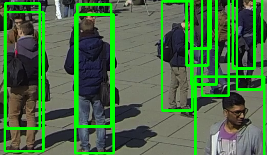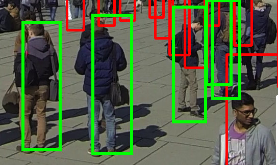
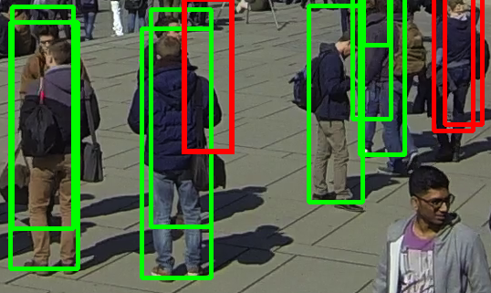
RCNN-2D/3D	POM-CNN	Ours

Figure 1: Multi-camera detection in a crowded scene. Even though there are 7 cameras with overlapping fields of view, baselines inspired by earlier approaches—-RCNN-2D/3D by [25] and POM-CNN by [10], as described in Section 7.2—both generate false positives denoted by red rectangles and miss or misplace a number of people, whereas ours does not. This example is representative of the algorithm’s behavior and is best viewed in color. Please see supplementary material for results on a video sequence.

Since then, Deep Learning based people detection algorithms in single images [21, 17, 26] have become among the most effective [26]. However, their power has only rarely been leveraged for MCMT purposes. Some recent algorithms, such as the one of [25], attempt to do so by first detecting people in single images, projecting the detections into a common reference-frame, and finally putting them into correspondence to achieve 3D localization and eliminate false positives. As shown in Fig. 1, this is prone to errors for two reasons. First, projection in the reference frame is inaccurate, especially when the 2D detector has not been specifically trained for that purpose. Second, the projection is usually preceded by Non Maximum Suppression (NMS) on the output of the 2D detector, which does not take into account the multi-camera geometry to resolve ambiguities.

Ideally, the power of Deep Learning should be combined with occlusion reasoning much earlier in the detection process than is normally done. To this end, we designed a joint CNN/CRF model whose posterior distribution can be approximated by Mean-Field inference using standard differentiable operations. Our model is trainable end-to-end and can be used in both supervised and unsupervised scenarios.

More specifically, we reason on a discretized ground plane in which detections are represented by boolean variables. The CRF is defined as a sum of innovative high-order terms whose values are computed by measuring the discrepancy between the predictions of a generative model that accounts for occlusions and those of a CNN that can infer that certain image patches look like specific body parts. To these terms, we add unary and pairwise ones to increase robustness and model physical repulsion constraints.

To summarize, our contribution is a joint CNN/CRF pipeline that performs detection for MCMT purposes in such a way that NMS is not required. Because it explicitly models occlusions, our algorithm operates robustly even in crowded scenes. Furthermore, it outputs probabilities of presence on the ground plane, as opposed to binary detections, which can then be linked into full trajectories using a simple flow-based approach [6].

2 Related Work

In this section, we first discuss briefly recent Deep Learning approaches to people detection in single images. We then move on to multi-image algorithms and techniques for combining CNNs and CRFs.

2.1 Deep Monocular Detection

As in many other domains, CNN-based algorithms [21, 17, 20] have become for very good for people detection in single images and achieve state-of-the-art performance [26]. Algorithms in this class usually first propose potential candidate bounding boxes with scores assigned to them. They then perform Non-Maximum Suppression (NMS) and return a final set of candidates. The very popular method of [21] performs both steps in a single CNN pass through the image. It returns a feature map in which a feature vector of constant dimension is associated to each image pixel. For any 2D bounding-box of any size in that image, a feature vector of any arbitrary dimension can then be computed using Region Of Interest (ROI) pooling and fed to a classifier to assess whether the bounding box does indeed correspond to a true detection.

While this algorithm has demonstrated its worth on many benchmarks, it can fail in crowded scenes such as the one of Fig. 1. This is perennial problem of single-image detectors when people occlude each other severely. One solution to this problem is to rely on cameras with overlapping fields of view, as discussed below.

2.2 Multi-Camera Pedestrian Detection

Here, we distinguish between recent algorithms that rely on Deep Learning but do not explicitly account for occlusions and older ones that model occlusions and geometry but appeared before the Deep Learning became popular. Our approach can be understood as a way to bring together their respective strengths.

The recent algorithm of [25] runs a monocular detector similar to the one of [21] on multiple views and infers people ground locations from the resulting detections. However, this method is prone to errors both because the 2D detections are performed independently of each other and because combining them by projecting them onto the ground plane involves reprojection errors and ignores occlusions. Yet, it is representative of the current MCMT state-of-the-art and is benchmarked against much older algorithms [10, 6] that rely on background subtraction instead of a Deep Learning approach.

These older algorithms use multiple cameras with overlapping fields of view to leverage geometrical or appearance consistency across views to resolve the ambiguities that arise in crowded scenes and obtain accurate 3D localisation [10, 1, 19]. They rely on Bayesian inference and graphical models to enforce detection sparsity. For example, the Probabilisitic Occupancy Map (POM) approach [10] takes background subtraction images as input and relies on Mean Field inference to compute probabilities of presence in the ground plane. More specifically, given several cameras with overlapping fields of view of a discretized ground plane, POM first performs background subtraction. It then uses a generative model that represents humans as simple rectangles in order to create synthetic ideal images that would be observed if people were at given locations. Under this model of the image given the true occupancy, it approximates the probabilities of occupancy at every location using Mean Field inference. Because the generative model explicitly accounts for occlusions, POM is robust and often performs well. But it relies on background subtraction results as its only input, which is not discriminative enough when the people density increases, as shown in Fig. 1. The algorithm of [1] operates on similar principles as POM but introduces more sophisticated human templates. Since it also relies on background subtraction, it is subject to the same limitations when the people density increases. And so is the algorithm of [19] that introduces a more complex Bayesian model to enhance the results of [1].

2.3 Combining CNNs and CRFs

Using a CNN to compute potentials for a Conditional Random Field (CRF) and training them jointly for structured prediction purposes has received much attention in recent years [16, 8, 9, 27, 2, 13, 15, 3]. However, properly training the CRFs remains difficult because many interesting models yield intractable inference problems. A popular workaround is to optimize the CRF potentials so as to minimize a loss defined on the output of an inference algorithm. Back Mean-Field [9, 27, 2, 15] has emerged as a promising way to do this. It relies on the fact that the updates steps during Mean-Field inference are continuous and parallelizable [4]. It is therefore possible to represent these operations as additional layers in a Neural Network and back-propagate through it. So far, this method has mostly been demonstrated either for toy problems or for semantic segmentation with attractive potentials, whereas our approach also requires repulsive potentials.

3 Modeling Occlusions in a CNN Framework

The core motivation behind our approach is to properly handle occlusions, while still leveraging the power of CNNs. To do so, we must model the interactions between multiple people who occlude each other but may not be physically close to each other. Our solution is to introduce an observation space; a generative model for observations given where people are located in the ground plane; and a discriminative model that predicts expected observations from the images. We then define a loss function that measures how different the CNN predictions are from those generated by the model. Finally, we use a Mean-Field approach with respect to probabilities of presence in the ground plane to minimize this loss. We cast this computation in terms of minimizing the energy of a Conditional Random Field in which the interactions between nodes are non-local because the people who occlude each other may not be physically close, which requires long range high-order terms.

In the remainder of this section, we first introduce the required notations to formalize our model. We then define a CRF that only involves high-order interaction potentials. Finally, we describe a more complete one that also relies on unary and pairwise terms.

3.1 Notations

We discretrize the ground plane in grid cells and introduce Boolean variables that denote the presence or absence of someone in the cell. Let us therefore consider a discretized ground plane containing $N$ locations. Let $Z_{i}$ be the boolean variable that denotes the presence of someone at location $i$. Let us assume we are given $C$ RGB images $I^{c}$ of size $H^{c}\times W^{c}$ from multiple views $1\leq c\leq C$ and $I=\{I^{1},\dots,I^{C}\}$. For each ground plane location $i$ and camera $c$, let the smallest rectangular zone containing the 2D projection of a human-sized 3D cylinder located at $i$ be defined by its top-left and bottom-right coordinates $T^{c}_{i}$ and $B^{c}_{i}$. For a pixel $k\in\{1,\dots,H^{c}\}\times\{1,\dots,W^{c}\}$, let $L^{c}_{k}$ be the set of such projections that contain $k$.

We also introduce a CNN that defines an operator $\mathcal{F}(\cdot;\theta_{F})$, which takes as input the RGB image of camera $c$ and outputs a feature map $\mathcal{F}^{c}=\mathcal{F}(I^{c};\theta_{F})$, where $\theta_{F}$ denotes the network’s parameters. It contains a $d$-dimensional vector $\mathcal{F}^{c}_{k}$ for each pixel $k$.

3.2 High-Order CRF

Figure 2: Schematic representation of our High-Order potentials as described in Section 3.2.2.

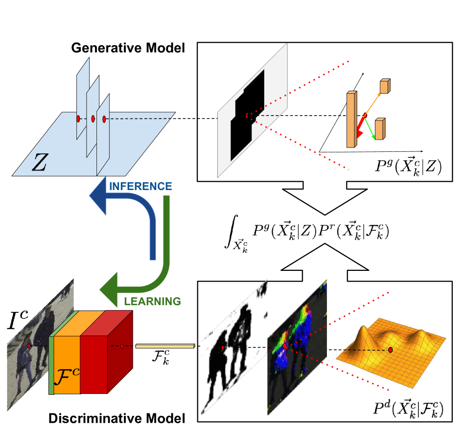
We take the energy of our CRF to be a sum of High-Order potentials $\psi^{c,k}_{\text{h}}$, one for each pixel. They handle jointly detection, and occlusion reasoning while removing the need for Non-Maximum Suppression. Each of these potentials use Probability Product Kernels [11] to represent the agreement between a generative model and a discriminative model over the observation space, at a given pixel, as depicted in Fig. 2. We therefore write

$$P(Z;I) = \dfrac{1}{\mathcal{Z}}\exp\psi_{\text{h}}(Z;\mathcal{F}(I;\theta_{F}))\;,$$ (1)

$$\psi_{\text{h}}(Z;\mathcal{F}) = \sum_{1\leq c\leq C,k\in\{1,\dots,H^{c}\}\times\{1,\dots,W^{c}\}}\psi^{c,k}_{\text{h}}(Z;\mathcal{F}^{c}_{k})\;.$$

Assuming we know the values of the occupancy variables $Z$, the generative model computes distributions over the set of observations. For each pixel in each image, it considers the corresponding line of sight and computes a distribution of vectors depending on the probability that it actually belongs to the successive people it traverses. This results in images whose pixels are vectors representing a distribution of 2D vectors, the observations, as depicted in the top row of Fig 2. Our discriminative model relies on a CNN which tries to predict similar distributions of 2D vectors, directly by looking at the image. For ease of understanding, we first present in more details a simple version of our High-Order potentials $\psi^{c,k}_{\text{h}}$. It assumes that our observations are zeros and ones at every pixel. The discriminative model therefore acts much as the background subtraction algorithms used in [10] did. We then extend them to take into account the 2D vector output of our discriminative model.

3.2.1 Simple Generative Model

We first introduce a binary observation variable $X^{c}_{k}\in\{0,1\}$ over which we define two distributions $P^{g}$ and $P^{d}$ produced by the generative and discriminative model respectively. We take the distribution $P^{g}$ to be

$$P^{g}(X^{c}_{k}=1|Z)=0, \mbox{ if }Z_{i}=0\;\forall i\in L^{c}_{k}\;,$$ (2)

$$P^{g}(X^{c}_{k}=1|Z)=1$$ otherwise,

and the discriminative one $P^{d}$ to be $P^{d}(X^{c}_{k}|\mathcal{F}^{c}_{k})=f_{\text{b}}(\mathcal{F}^{c}_{k};\theta_{b})$, where $F^{c}_{k}$ is the $d$-dimensional feature vector associated to pixel $k$ introduced above and $f_{\text{b}}$ is a Multi-Layer Perceptron (MLP) with weights $\theta_{b}$. In other words, $f_{\text{b}}$ plays the role of a CNN-based semantic segmentor or background-subtraction.

For each pixel, we then take the high-order potential to be the dot product between the distributions

$$\psi^{c,k}_{\text{h}}(Z;\mathcal{F}^{c}_{k})=\mu_{\text{h}}\log\int\limits_{\text{\hbox to0.0pt{\hss$X^{c}_{k}\in\{0,1\}$\hss}}}P^{g}(X^{c}_{k}|\{Z_{i}\}_{i\in L^{c}_{k}})P^{d}(X^{c}_{k}|\mathcal{F}^{c}_{k})\;,$$ (3)

as in the probability product kernel method of [11]. Intuitively, $\psi^{c,k}_{\text{h}}$ is high when the segmentation produced by the network matches the projection of the detections in each camera plane using the simple generative model of Eq. 2. $\mu_{\text{h}}$ is an energy scaling parameter.

3.2.2 Full Generative Model

The above model correctly accounts for occlusions and geometry but ignores much image information by focusing on background / foreground decisions. To refine it, we model the part of the bounding-box a pixel belongs to rather than just the fact that it belongs to a bounding-box. To this end, we redefine the Boolean auxiliary variable $X^{c}_{k}$ as

$$\vec{X}^{c}_{k}\in\{0\}\cup\mathbb{R}^{2}\;,$$ (4)

where the label $0$ represents background as before, and a label in $\mathbb{R}^{2}$ denotes the displacement with respect to the center of the body of the visible person at this pixel location.

To extend the simple model and account for what part of a bounding-box pixel $k$ belongs to if it does, we sample from the distribution $P^{g}(\vec{X}^{c}_{k}|\{Z_{i}\}_{i\in L^{c}_{k}})$. To this end, let us assume without loss of generality that the $L^{c}_{k}$ are ordered by increasing distance to the camera, as shown in the top left corner of Fig. 2. We initialize the variables $\vec{X}^{c}_{k}$ to 0. Then, for each $i$ in $L^{c}_{k}$ such that $Z_{i}=1$, we draw a boolean random variable $O_{i}$ with fixed expectancy $o$. If $O_{i}=1$, then

$$\vec{X}_{k} = \vec{x}^{i}_{k}\;,$$

$$= \left(\dfrac{k_{x}-0.5({T^{c}_{i}}_{x}+{B^{c}_{i}}_{x})}{{B^{c}_{i}}_{x}-{T^{c}_{i}}_{x}};\dfrac{k_{y}-0.5({T^{c}_{i}}_{y}+{B^{c}_{i}}_{y})}{{B^{c}_{i}}_{y}-{T^{c}_{i}}_{y}}\right)\;,$$

that is, the relative location of pixel $k$ with respect to the projection of detection $i$ in camera $c$, as depicted in the upper right corner of Fig. 2.

We define the distribution $P^{d}(\vec{X}_{k}|\mathcal{F}^{c}_{k})$ as an $M$-Modal Gaussian Mixture

$$P^{d}(\vec{X}_{k}=0) =f_{\text{b}}(\mathcal{F}^{c}_{k};\theta_{b})\;,$$ (6)

$$P^{d}(\vec{X}_{k}|\vec{X}_{k}\neq 0) =\sum\limits_{1\leq m\leq M}f_{\text{h}}(\mathcal{F}^{c}_{k};\theta_{\text{h}})_{m}\mathcal{N}(\vec{X}_{k}-\alpha_{m};\sigma_{m})\;,$$

as depicted in the bottom right corner of Fig. 2. As a result, $P^{d}(\vec{X}_{k}=0)$ is the same as in the simple model but $P^{d}(\vec{X}_{k}|\vec{X}_{k}\neq 0)$ encodes more information. $(\alpha_{m},\sigma_{m})$ are Gaussian parameters learned for each mode $m$. $f_{\text{h}}$ is a MLP parametrized by $\theta_{\text{h}}$ that outputs $M$ normalized real probabilities where M is a meta-parameter of our model. Similarly, $f_{\text{b}}(\mathcal{F}^{c}_{k};\theta_{b})$ is a background probability.

Finally, as in Eq. 3, we take our complete potential to be

$$\psi^{c,k}_{\text{h}}(Z;\mathcal{F}^{c}_{k})=\mu_{\text{h}}\log\int\limits_{\text{\hbox to0.0pt{\hss$\vec{X}_{k}\in\{0\}\cup\mathbb{R}^{2}$\hss}}}P^{g}(\vec{X}_{k}|\{Z_{i}\}_{i\in L^{c}_{k}})P^{d}(\vec{X}_{k}|\mathcal{F}^{c}_{k})\;.$$ (7)

3.3 Complete CRF

To increase the robustness of our CRF, we have found it effective to add, to the high-order potentials of Eq. 1, unary and pairwise ones to exploit additional image information. We therefore write our complete CRF model as

$$P(Z;I) = \dfrac{1}{\mathcal{Z}}\exp\psi(Z;\mathcal{F})\;,$$ (8)

$$\psi(Z;\mathcal{F}) = \psi_{\text{h}}(Z;\mathcal{F})+\sum_{i\leq N}\psi^{i}_{\text{u}}(Z_{i};\mathcal{F})+\sum_{i\leq N,j\leq N}\psi_{\text{p}}(Z_{i},Z_{j}),$$

where $\psi_{\text{h}}$ is the high-order CRF of Eq. 1, the $\psi^{i}_{\text{u}}$ are unary potentials, and $\psi_{\text{p}}$ pairwise ones, which we describe below.

3.3.1 Unaries

The purpose of our unary potentials is to provide a prior probability of presence at a given location on the ground, before considering the occlusion effect and non maximum suppression. For each location $i$ and camera $c$, we use a CNN $f_{\text{u}}(T^{c}_{i},B^{c}_{i},\mathcal{F}^{c})$, which outputs a probability of presence of a person at location $i$. $f_{\text{u}}$ works by extracting a fixed size feature vector from the rectangular region defined by $T^{c}_{i},B^{c}_{i}$ in $\mathcal{F}^{c}$, using an ROI pooling layer [21]. A detection probability is finally estimated using an MLP. Estimates from the multiple cameras are pooled through a $max$ operation

$$\psi^{i}_{\text{u}}(Z_{i};\mathcal{F})=\mu_{\text{u}}Z_{i}\max_{c}\log\dfrac{f_{\text{u}}(T^{c}_{i},B^{c}_{i},\mathcal{F}_{c})}{1-f_{\text{u}}(T^{c}_{i},B^{c}_{i},\mathcal{F}_{c})}\;,$$ (9)

where $\mu_{\text{u}}$ is a scalar that controls the importance of unary terms compared to others.

3.3.2 Pairwise

The purpose of our pairwise potentials is to represent the fact that two people are unlikely to stand too close to each others. For all pairs of locations $(i,j)$, let $E^{i,j}_{\text{p}}=E_{\text{p}}[|x_{i}-x_{j}|;|y_{i}-y_{j}|]$, where $E_{\text{p}}$ is a 2D kernel function of of predefined size. We write

$$\psi_{\text{p}}(Z_{i},Z_{j})=-E^{i,j}_{\text{p}}Z_{i}Z_{j}$$ (10)

for locations that are closer to each other than a predefined distance and 0 otherwise.

4 Inference and Derivation

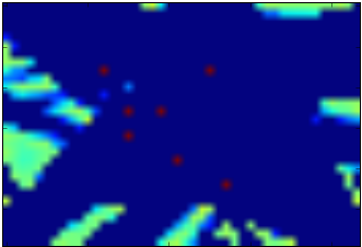
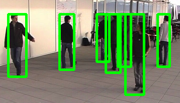
Given the CRF of Eq. 8 and assuming all parameters known, finding out where people are in the ground plane amounts to minimizing $\psi$ with respect to $Z$, the vector of binary variables that indicates which ground locations contain someone, which amounts to computing a Maximum-a-Posteriori of the posterior $P$. Instead of doing so directly, which would be intractable, we use Mean-Field inference [24] to approximate of $P$ by a fully-factorised distribution $Q$. As in [10], this produces a Probability Occupancy Map, that is, a probability of presence $Q(Z_{i}=1)$, at each location, such as the one depicted by Fig. 3.

(a) (b)

Figure 3: Output. (a) Given a set of images of the same scene, ours algorithm produces a Probabilistic Occupancy Map, that is, a probability of presence at each location of the ground plane. Red values indicate probabilities close to 1 and blue ones values close to zero. (b) Because the probabilities are very peaked, they can easily be thresholded to produce detections whose projections are the green boxes in the original image(s).

To perform this minimization, we rely on the natural-gradient descent scheme of [4]. It involves taking gradient steps that are proportional to

$$\nabla_{\eta_{i}}=\mathbb{E}_{Q}\left[\left(\psi(Z,\mathcal{F})\right)|Z_{i}=1\right]-\mathbb{E}_{Q}\left[\left(\psi(Z,\mathcal{F})\right)|Z_{i}=0\right],$$ (11)

for each location $i$. The contribution to $\nabla_{\eta_{i}}$ of the unaries derives straightforwardly from Eq. 9. Similarly, the one of the pairwise potentials of Eq. 10 is

$$(\nabla_{\eta_{i}})_{\text{p}} =-\sum_{j}E^{i,j}_{\text{p}}Q_{j}(Z_{j}=1)\;,$$ (12)

$$=-\sum_{j}E_{\text{p}}[|x_{i}-x_{j}|,|y_{i}-y_{j}|]Q_{j}(Z_{j}=1)\;,$$

which can be implemented as a convolution over the current estimate of the probabilistic occupancy map $Q$ with the two dimensional kernel $E_{\text{p}}[.,.]$. This makes it easy to unroll the inference steps using a Deep-Learning framework.

Formulating the contributions of the higher-order terms of Eq. 7 is more involved and requires simplifications. We first approximate the Gaussians used in Eq. 6 by a function whose value is $1$ in $B_{m}$ and $\epsilon$ elsewhere, where $B_{m}$ is the rectangle of center $\alpha_{m}$ and half-size $3\sigma_{m}$. Note that this approximation is only used for inference purposes, and that during training, it keeps its original Gaussian form. We then threshold the Gaussian weights $f_{\text{h}}$ resulting in the binary approximation $\tilde{f}_{\text{h}}$. This yields a binary approximation $\widetilde{R}_{\text{h}}(\vec{X}_{k})$ of $R_{\text{h}}(\vec{X}_{k})$. Note that the corresponding approximate potential $\widetilde{\psi}^{c,k}_{\text{h}}(Z,\mathcal{F}^{c}_{k})$ can be either $O(\log\epsilon)$, if $P(\vec{X}_{k},b_{k}=1;Z)=0$ for all $\vec{X}_{k}$ such that $R_{\text{h}}(\vec{X}_{k})>\epsilon$ or $O(\log(1))$. Hence, the configurations where $\psi^{c,k}_{\text{h}}(Z,\mathcal{F}^{c}_{k})=O(\log\epsilon)$ will dominate the others when computing the expectancies. This yields the approximation of Eq. 11,

$$\widetilde{\nabla\eta_{i}}=-C(\mathbb{E}_{Q}\left[\Delta(Z)|Z_{i}=1\right]-\mathbb{E}_{Q}\left[\Delta(Z)|Z_{i}=0\right])\;,$$ (13)

where $C=-log{\epsilon}$ is a constant and $\Delta(Z)$ is a binary random variable, which takes value 1 if $\widetilde{\psi}^{c,k}_{\text{h}}(Z,\mathcal{F}^{c}_{k})=0$, and 0 otherwise. Note that $\psi^{c,k}_{\text{h}}(Z,\mathcal{F}^{c}_{k})=O(\log(1))$ iff

$$\exists i\leq N,m\leq M\mbox{ s.t }\widetilde{f}_{\text{h}}(\mathcal{F}^{c}_{k};\theta_{\text{h}})_{m}=1\text{ and }\vec{X}^{i}_{k}\in B_{m}\;.$$ (14)

This means that for each pixel $k$, given a thresholded output from the network $\widetilde{f}_{\text{h}}(\mathcal{F}^{c}_{k};\theta_{\text{h}})$, we obtain a list of compatible explanations $\mathcal{C}_{k}\subset\{1,\dots,N\}$ such that pixel $k$ defines a very simple pattern-based potential of the form $1$ if $Z_{i}=0\;\forall i\in\mathcal{C}_{k}$, $0$ otherwise, which is similar to the potentials used in the Mean-Fields algorithms of [23, 10, 14, 2, 5]. In the supplementary material, we see how this operation can be implemented efficiently using common Deep-Learning operations and integral-images.

5 Training

We now show how our model can be trained first in a supervised manner and then in an unsupervised one.

5.1 Supervised Training

Let us first assume that we observe $D$ data point $(Z^{0},I^{0}),\dots,(Z^{D},I^{D})$, where $I^{d}$ represents a multi-view image and $Z^{d}$ the corresponding ground truth presences. The purpose of training is then to optimize the network parameters $\theta_{F},\theta_{\text{u}},\theta_{\text{h}}$ defined in Sections 3.1, 3.3.1 and 3.2.2 respectively, the gaussian parameters $\alpha,\sigma$ of Eq. 6 and the energy-scaling meta-parameters $\mu_{\text{u}},\mu_{\text{h}}$ of Eqs. 9 and 3 to maximize $\sum\limits_{d\leq D}\log P(Z^{d};I^{d})$. It cannot be done directly using Eq. 8 because computing the partition function $\mathcal{Z}$ is intractable.

Back Mean-Field

An increasingly popular work-around is to optimize the above-mentioned parameters to ensure that the output of the Mean-Field inference fits the ground truth. In other terms, let $Q_{\theta_{F},\theta_{\text{u}},\theta_{\text{h}},\alpha,\sigma}(Z;I)$ be the distribution obtained after inference . We look for

$$\operatorname*{\arg\!\max}_{\theta_{F},\theta_{\text{u}},\theta_{\text{h}},\alpha,\sigma}\sum_{(Z^{d},I^{d})}\log Q_{\theta_{F},\theta_{\text{u}},\theta_{\text{h}},\alpha,\sigma}(Z=Z^{d};I^{d})\;.$$ (15)

Since $Q_{\theta_{F},\theta_{\text{u}},\theta_{\text{h}},\alpha,\sigma}(Z=Z^{d};I^{d})$ is computed via a sequence of operations which are all differentiable with respect to the parameters $\theta_{F},\theta_{\text{u}}$, and $\theta_{\text{h}}$, it is therefore possible to solve Eq. 15 by stochastic gradient descent [9, 27].

Pre-training

However, it still remains difficult to optimize the whole model from scratch. We therefore pre-train our potentials separately before end-to-end fine-tuning. More precisely, the CNN $f_{\text{u}}$ that appears in the unary terms of Eq. 9 is trained as a standard classifier that gives the probability of presence at a given location, given the projection of the corresponding bounding-box in each camera view. For each data point, this leaves the high-order terms for which we need to optimize

$$\sum_{c}\sum_{k\in\mathcal{P}_{c}}\log(\psi^{c,k}_{\text{h}}(Z^{d},\mathcal{F}^{c}_{k}))\;,$$ (16)

with respect to the parameters of the Gaussian Mixture network $\theta_{\text{h}},\alpha$, and $\sigma$. We use Jensen’s inequality to take our generative distribution $P^{g}$ out of the integral in Eq. 7 and approximate it by random sampling procedure described in Section 3.2.2. We rewrite the set of samples for $\vec{X}^{c}_{k}$ from all the pixels from all the cameras from all the data-points as $S(Z^{0},\dots,Z^{D})$. The optimization objective of Eq. 16 can then be rewritten as

$$\sum_{\vec{x}_{s}\in S(Z^{0},\dots,Z^{D})}\log(P^{d}(\vec{x}_{s}|\mathcal{F}^{c}_{k},\theta_{\text{h}},\alpha,\sigma))\;,$$ (17)

which is optimized by alternating a standard stochastic gradient descent for the $\theta_{\text{h}}$ parameters and a closed form batch optimization for $\alpha,\sigma$. This procedure is similar to one often used to fit a Mixture of Gaussians, except that, during the E-Step, instead of computing the class probabilities directly to increase the likelihood, we optimise the parameters of the network through gradient descent. More details are provided in the supplementary material.

This pre-training strategy creates potentials which are reasonable but not designed to be commensurate with each others. We therefore need to choose the two energy parameters scalars $\mu_{\text{u}}$, and $\mu_{\text{h}}$, via grid-search in order to optimize the relative weights of Unary and High-Order potentials before using the Back-Mean field method.

5.2 Unsupervised Training

In the absence of annotated training data, inter-view consistency and translation invariance still provide precious a-priori information, which can be leveraged to train our model in an unsupervised way.

Let us assume that the background-subtracting part of the network, which computes ${f_{\text{b}}}$, the MLP introduced in Section 3.2.2, is reasonably initialized. In practice, it is easy to do either by training it on a segmentation dataset or by relying on simple background subtraction to compute $f_{\text{b}}$. Then, starting from initial values of the parameters $\theta$, we first compute the Mean-Field approximation of $P(Z;I_{0},\theta)$, which gives us a first lower bound of the partition function. We then sample $Z$ from $Q$ and use that to train our potentials separately as if these samples were ground truth-data, using the supervised procedure of Section 5.1. We then iterate this procedure, that is, Mean-Field inference, sampling from $Z$, and optimizing the potentials sequentially. This can be interpreted as an Expectation-Maximization (EM) [7] procedure to optimize an Expected Lower Bound (ELB) to the partition function $\mathcal{Z}$ of Eq. 8.

6 Implementation Details

Our implementation uses a single VGGNet-16 Network with pre-trained weights. It computes features that will then be used to estimate both unary and pairwise potentials. The features map $\mathcal{F}^{c}=\mathcal{F}(I^{c};\theta_{F})$ is obtained by upsampling of the convolutional layers.

Similarly to the classification step in [21], we restrict the Region-Of-Interest pooling layer (ROI) to the features from the last convolutional layer of VGGNet. The output of the ROI is a 3x3x1024 tensor, which is flattened and input to a two layers MLP with ReLU non-linearities. In a similar way as in previous works on segmentation [27], we use a two layers MLP to classify each hyper-column of our dense features map $\mathcal{F}^{c}=\mathcal{F}(I^{c};\theta_{F})$ to produce segmentation $f_{\text{b}}$ and Gaussian Class $f_{\text{h}}$ probabilities.

We use $M=8$ modes for Multi-Modal Gaussian distribution of Eq. 6 for all our experiments and we have not assessed the impact of this choice on the performance. Besides, our kernel defining the pairwise potentials of Eq. 10 takes an arbitrary uniform constant value. For unsupervised training, we use a fixed number of $6$ EM iterations, which we empirically found to be enough, as illustrated in the supplementary material.

Finally, all our pipeline is implemented end-to-end using standard differentiable operations from the Theano Deep-Learning library [22]. For Mean-Field inference, we use a fixed number of iterations (30) and step size (0.01).

7 Evaluation

7.1 Datasets, Metrics, and Baselines

We introduce here the datasets we used for our experiments, the metrics we relied on to evaluate performance, and the baselines to which we compared our approach.

Datasets.

• ETHZ. It was acquired using 7 cameras to film the dense flow of students in front of the ETHZ main building in Zürich for two hours. It comprises 250 annotated temporal 7-image frames in which up to 30 people can be present at a time. We used 200 of these frames for training and validation and 50 for evaluation. See the image of Fig. 1 for a visualization.

• EPFL. The images were acquired at 25 fps on the terrace of an EPFL building in Lausanne using 4 DV cameras. The image of Fig. 3 is one of them. Up to 7 people walk around for about 3 1/2 minutes. As there are only 80 annotated frames, we used them all for evaluation purposes and relied either on pre-trained models or unsupervised training.

• PETS. The standard PETS 2009 (PETS S2L1) is widely used for monocular and multi-camera detection. It contains 750 annotated images and was acquired from 7 cameras. It is a simple dataset in the sense that it is not very crowded, but the calibration is inaccurate and the image quality low.

Metrics.

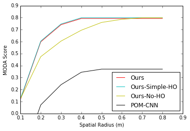
Recall from Section 4, that our algorithms produces Probabilistic Occupancy Maps, such as the ones of Fig. 3. They are probabilities of presence of people at ground locations and are very peaky. We therefore simply label locations where the probability of presence is greater than $0.5$ as being occupied and will refer to these as detections, without any need for Non-Maximum suppression. We compute false positive (FP), false negative (FN) and true positives (TP) by assigning detections to ground truth using Hungarian matching. Since we operate in the ground plane, we impose that a detection can be assigned to a ground truth annotation only if they are less than a distance $r$ away. Given FP, FN and TP, we can evaluate:

• Multiple Object Detection Accuracy (MODA) which we will plot as a function of $r$, and the Multiple Object Detection Precision (MODP)  [12].

• Precision-Recall. Precision and Recall are taken to be TP/(TP + FN) and TP/(TP+FP) respectively.

We will report MODP, Precision, and Recall for $r=0.5$, which roughly corresponds to the width of a human body. Note that these metrics are unforgiving of projection errors because we measure distances in the ground plane, which would not be the case if we evaluated overlap in the image plane as is often done in the monocular case. Nevertheless, we believe them to be the metrics for a multi-camera system that computes the 3D location of people.

ETHZ	EPFL	PETS

	ETHZ		EPFL		PETS
Method	Precision / Recall	MODP	Precision / Recall	MODP	Precision / Recall	MODP
Ours	95 / 80%	53.8%	-	-	-	-
Ours-No-FT	93 / 80%	53.4%	88 / 82%	48.3%	93 / 87%	60.4%
Ours-Unsuperv	86 / 80%	49.8%	80 / 85%	47.5%	-	-
Ours-Simple-HO	87 / 70%	47.5%	85 / 75%	43.2%	93 / 87%	60.4%
Ours-No-HO	84 / 55%	34.4%	37 / 68%	23.3%	93 / 81%	55.2%
POM-CNN	75 / 55%	30.5%	80 / 78%	45.9%	90 / 86%	42.9%
RCNN-2D/3D	68 / 43%	18.4%	39 / 50%	21.6%	50 / 63%	27.6%

Figure 4: Results on our three test datasets. Top row. MODA scores for the different methods as function of the radius $r$ used to compute it, as discussed in Section 7.1. Bottom row. Precision/Recall and MODP for the different methods for $r=0.5$. Some of the values are absent either due to the bad calibration of the data-set, or missing ground-truth, as explained in Sections 7.1 and 7.2. The numbers we report for the RCNN-2D/3D baseline are much lower than those reported in [25] for the method that inspired it, in large part because we evaluate our metrics in the ground plane instead of the image plane and because [25] uses a temporal consistency to improve detections.

Baselines and Variants of our Method.

We implemented the following two baselines.

• POM-CNN. The multi-camera detector [10] described in Section 2.2 takes background subtraction images as its input. In its original implementation, they were obtained using traditional algorithms [28, 18]. For a fair comparison reflecting the progress that has occurred since then, we use the same CNN-based segmentor as the one use to segment the background, that is $f_{\text{b}}(\mathcal{F}^{c}_{k};\theta_{b})_{0}$ from Eq. 6.

• RCNN-2D/3D. The recent work of [25] proposes a MCMT tracking framework that relies on a powerful CNN for detection purposes [21], as discussed in Section 2.2. Since the code of [25] is not publicly available, we reimplemented their detection methodology as faithfully as possible but without the tracking component for a fair comparison with our approach that operates on images acquired at the same time. Specifically, we run the 2D detector [21] on each image. We then project the bottom of the 2D bounding box onto the ground reference frame as in [25] to get 3D ground coordinates. Finally, we cluster all the detections from all the cameras using 3D proximity to produce the final set of detections.

To gauge the influence of the different components or our approach, we compared these baselines against the following variants of our method.

• Ours. Our method with all three terms in the CRF model turned on, as described in Section 3.3, and fine tuned end-to-end through back Mean-Field, as described in Section 5.1.

• Ours-No-FT. Ours without the final fine-tuning.

• Ours-Unsuperv. Same as Ours-No-FT but the training is done without ground truth annotations, as described in Section 5.2.

• Ours-Simple-HO : We replace the full High-Order term of Section 3.2 with the simplified one that approximates the one of [10], as described at the beginning of that section.

• Ours-No-HO. We remove the High-Order term of Section 3.2 altogether.

7.2 Results

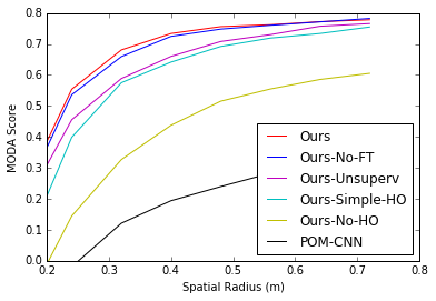
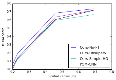
We report our results on our three test datasets in Fig. 4.

ETHZ.

Ours and Ours-No-FT clearly dominate the RCNN-2D/3D and POM-CNN baselines, with Ours slightly outperforming Ours-No-FT because of the fine-tuning. Simplifying the high-order term, as in Ours-Simple-HO, degrades performance and removing it, as in Ours-No-HO, degrades it even more. The methods discussed above rely on supervised training, whereas Ours-Unsuperv does not but still outperforms the baselines.

EPFL.

Because the images have different statistics than those of ETHZ, the unary terms as well as the people detector RCNN-2D/3D relies on are affected. And since there is no annotated data for retraining, as discussed above, the performance of Ours-No-HO and RCNN-2D/3D drop very significantly with respect to those obtained on ETHZ. By contrast, the high order terms are immune to this, and both Ours-No-FT and Ours-Unsuperv hold their performances.

PETS.

The ranking of the methods is the same as before except for the fact that Ours-Simple-HO does as well as Ours-No-FT. This is because the PETS dataset is poorly calibrated, which results in inaccurate estimates of the displacement vectors in the generative model of Section 3.2.2. As a result, it does not deliver much of a performance boost and we therefore did not find it meaningful to report results for unsupervised training and fine-tuning of these High-Order potentials.

From Detections to Trajectories.

Since our method produces a Probability Occupancy Map for every temporal frame in our image sequences, we can take advantage of a simple-flow based method [6] to enforce temporal consistency and produce complete trajectories. As shown in Fig. 5 this leads to further improvements for all three datasets.

Method	ETHZ	EPFL	PETS
Ours	74.1%	68.2%	79.8%
Ours + [6]	75.2%	76.9%	83.4%

Figure 5: MODA scores for $r=0.5$ before and after enforcing temporal consistency.

8 Discussion

We introduced a new CNN/CRF pipeline that outperforms the state-of-the art for multi-camera people localization in crowded scenes. It handles occlusion while taking full advantage of the power of a modern CNN and can be trained either in a supervised or unsupervised manner.

A limitation, however, is that the CNN used to compute our unary potentials still operates in each image independently as opposed to pooling very early the information from multiple images and then leveraging the expected appearance consistency across views. In future work, we will therefore investigate training such a CNN for people detection on multiple images simultaneously, jointly with our CRF.

References

- [1] A. Alahi, L. Jacques, Y. Boursier, and P. Vandergheynst. Sparsity Driven People Localization with a Heterogeneous Network of Cameras. Journal of Mathematical Imaging and Vision, 2011.
- [2] A. Arnab, S. Jayasumana, S. Zheng, and P. H. S. Torr. Higher Order Potentials in End-To-End Trainable Conditional Random Fields. CoRR, abs/1511.08119, 2015.
- [3] T. Bagautdinov, A. Alahi, F. Fleuret, P. Fua, and S. Savarese. Social Scene Understanding: End-To-End Multi-Person Action Localization and Collective Activity Recognition. In Conference on Computer Vision and Pattern Recognition, 2017.
- [4] P. Baque, T. Bagautdinov, F. Fleuret, and P. Fua. Principled Parallel Mean-Field Inference for Discrete Random Fields. In Conference on Computer Vision and Pattern Recognition, 2016.
- [5] P. Baque, F. Fleuret, and P. Fua. Multi-Modal Mean-Fields via Cardinality-Based Clamping. In Conference on Computer Vision and Pattern Recognition, 2017.
- [6] J. Berclaz, F. Fleuret, E. Türetken, and P. Fua. Multiple Object Tracking Using K-Shortest Paths Optimization. IEEE Transactions on Pattern Analysis and Machine Intelligence, 33(11):1806–1819, 2011.
- [7] D. Blei, A. Kucukelbir, and J. McAuliffe. Variational inference: A review for statisticians. 2016.
- [8] T.-M.-T. Do and T. Artieres. Neural conditional random fields. In Proceedings of the Thirteenth International Conference on Artificial Intelligence and Statistics, volume 9. JMLR, 5 2010.
- [9] J. Domke. Learning Graphical Model Parameters with Approximate Marginal Inference. CoRR, abs/1301.3193, 2013.
- [10] F. Fleuret, J. Berclaz, R. Lengagne, and P. Fua. Multi-Camera People Tracking with a Probabilistic Occupancy Map. IEEE Transactions on Pattern Analysis and Machine Intelligence, 30(2):267–282, February 2008.
- [11] T. Jebara, R. Kondor, and A. Howard. Probability Product Kernels. J. Mach. Learn. Res., 5, 2004.
- [12] R. Kasturi, D. Goldgof, P. Soundararajan, V. Manohar, J. Garofolo, M. Boonstra, V. Korzhova, and J. Zhang. Framework for Performance Evaluation of Face, Text, and Vehicle Detection and Tracking in Video: Data, Metrics, and Protocol. IEEE Transactions on Pattern Analysis and Machine Intelligence, 31(2):319–336, 2009.
- [13] A. Kirillov, D. Schlesinger, S. Zheng, B. Savchynskyy, P. Torr, and C. Rother. Joint Training of Generic CNN-CRF Models with Stochastic Optimization. arXiv Preprint, 2015.
- [14] P. Kohli and C. Rother. Higher-Order Models in Computer Vision. In O. Lezoray and L. Grady, editors, Image Processing and Analysis with Graphs, pages 65–100. CRC Press, 2012.
- [15] M. Larsson, F. Kahl, S. Zheng, A. Arnab, P. Torr, and R. Hartley. Learning Arbitrary Potentials in CRFs with Gradient Descent. arXiv Preprint, 2017.
- [16] Y. LeCun, S. Chopra, and R. Hadsell. A tutorial on energy-based learning. Predicting Structured Data, 2006.
- [17] W. Liu, D. Anguelov, D. Erhan, C. Szegedy, S. E. Reed, C.-Y. Fu, and A. C. Berg. SSD: Single Shot Multibox Detector. CoRR, abs/1512.02325, 2016.
- [18] N. Oliver, B. Rosario, and A. Pentland. A Bayesian Computer Vision System for Modeling Human Interactions. IEEE Transactions on Pattern Analysis and Machine Intelligence, 22(8):831–843, 2000.
- [19] P. Peng, Y. Tian, Y. Wang, J. Li, and T. Huang. Robust Multiple Cameras Pedestrian Detection with Multi-View Bayesian Network. Pattern Recognition, 48(5):1760–1772, 2015.
- [20] J. Redmon, S. Divvala, R. Girshick, and A. Farhadi. You Only Look Once: Unified, Real-Time Object Detection. In Conference on Computer Vision and Pattern Recognition, 2016.
- [21] S. Ren, K. He, R. Girshick, and J. Sun. Faster R-CNN: Towards Real-Time Object Detection with Region Proposal Networks. In Advances in Neural Information Processing Systems, 2015.
- [22] Theano Development Team. Theano: A Python framework for fast computation of mathematical expressions. arXiv e-prints, abs/1605.02688, May 2016.
- [23] V. Vineet, J. Warrell, and P. Torr. Filter-Based Mean-Field Inference for Random Fields with Higher-Order Terms and Product Label-Spaces. International Journal of Computer Vision, 110(3):290–307, 2014.
- [24] M. Wainwright and M. Jordan. Graphical Models, Exponential Families, and Variational Inference. Foundations and Trends in Machine Learning, 1(1-2):1–305, January 2008.
- [25] Y. Xu, X. Liu, Y. Liu, and S. Zhu. Multi-View People Tracking via Hierarchical Trajectory Composition. In Conference on Computer Vision and Pattern Recognition, pages 4256–4265, 2016.
- [26] S. Zhang, R. Benenson, M. Omran, J. Hosang, and B. Schiele. How Far Are We from Solving Pedestrian Detection? In Conference on Computer Vision and Pattern Recognition, pages 1259–1267, 2016.
- [27] S. Zheng, S. Jayasumana, B. Romera-paredes, V. Vineet, Z. Su, D. Du, C. Huang, and P. Torr. Conditional Random Fields as Recurrent Neural Networks. In International Conference on Computer Vision, 2015.
- [28] F. Ziliani and A. Cavallaro. Image Analysis for Video Surveillance Based on Spatial Regularization of a Statistical Model-Based Change Detection. In International Conference on Image Analysis and Processing, 1999.