Rate-Distortion Theory of Finite Point Processes

Abstract

We study the compression of data in the case where the useful information is contained in a set rather than a vector, i.e., the ordering of the data points is irrelevant and the number of data points is unknown. Our analysis is based on rate-distortion theory and the theory of finite point processes. We introduce fundamental information-theoretic concepts and quantities for point processes and present general lower and upper bounds on the rate-distortion function. To enable a comparison with the vector setting, we concretize our bounds for point processes of fixed cardinality. In particular, we analyze a fixed number of unordered Gaussian data points and show that we can significantly reduce the required rates compared to the best possible compression strategy for Gaussian vectors. As an example of point processes with variable cardinality, we study the best possible compression of Poisson point processes. For the specific case of a Poisson point process with uniform intensity on the unit square, our lower and upper bounds are separated by only a small gap and thus provide a good characterization of the rate-distortion function.

I Introduction

The continuing growth of the amount of data to be stored and analyzed in many applications calls for efficient methods for representing and compressing large data records [1]. In the literature on data compression, one aspect was hardly considered: the fact that we are often interested in sets and not in ordered lists, i.e., vectors, of data points. Our goal in this paper is to study the optimal compression of finite sets, also called point patterns, in an information-theoretic framework. More specifically, we consider a sequence of independent and identically distributed (i.i.d.) point patterns, and we want to calculate the minimal rate—i.e., number of representation bits per point pattern—for a given upper bound on the expected distortion. For this analysis, we need distributions on point patterns. Fortunately, these and other relevant mathematical tools are provided by the theory of (finite) point processes (PPs) [2, 3].

The theory and applications of PPs have a long history, and in most fields using this concept—such as, e.g., forestry [4], epidemiology [5], and astronomy [6]—significant amounts of data in the form of point patterns are collected, stored, and processed. Thus, we believe that lossy source coding may be of great interest in these fields. Furthermore, the recently studied problem of super-resolution [7, 8] or more generally atomic norm minimization [9] results in a point pattern in a continuous alphabet and is often described by some statistical properties. In this setting, one frequently deals with noisy signals, and thus an additional distortion resulting from lossy compression may be acceptable.

As a more explicit example, consider a database of minutiae patterns in fingerprints [10, 11]. Minutiae are endpoints and bifurcations of ridge lines on the finger. Typical data consists of $x$- and $y$-positions of points in some relative coordinate system and may well include further information such as the angle of the orientation field at the minutiae or the minutia types. For simplicity, we consider here only the positions; any additional information can be incorporated by a suitable adaptation of the distortion measure. A fingerprint of good quality typically contains about 40–100 minutiae [10]. For many minutia-based algorithms for fingerprint matching, the order in which the minutiae are stored is irrelevant [11] and a fingerprint can thus be represented as a point pattern. Furthermore, different pressures applied during the acquisition of a fingerprint lead to varying local deformations and thus varying minutiae for the same finger. Hence, in most applications, a small additional distortion due to compression will be acceptable. Because the exact locations as well as the number of minutiae acquired for the same finger may vary, the squared OSPA metric as defined further below in (LABEL:eq:ospagen) appears well suited for measuring the distortion between minutiae patterns.

I-A Prior Work

Information-theoretic work on PPs is scarce. An extension of entropy to PPs is available [3, Sec. 14.8], but apparently the mutual information between PPs was never analyzed in detail (although it is defined by the general quantization-based definition of mutual information [12, eq. (8.54)] or its equivalent form in (15) below). A similar quantity was recently considered for a special case in [13, Th. VI.1]. However, this quantity deviates from the general definition of mutual information, because the joint distribution in [13, eq. (5)] implies a fixed association between the points in the two PPs involved.

Source coding results for PPs are available almost exclusively for (infinite) Poisson PPs on $\mathbb{R}$ [14, 15, 16, 17]. However, that setting considers only a single PP rather than an i.i.d. sequence of PPs. More specifically, the sequence considered for rate-distortion (RD) analysis in [14, 15, 16, 17] is the growing vector of the smallest $n$ points of the PP. This approach was also adopted in [18], where the motivation was similar to that of the present paper but the main objective was to study the asymptotic behavior of the RD function as the cardinality of the data set grows infinite. It was shown in [18] that the expected distortion divided by the number of points in the data set converges to zero even for zero-rate coding. Although we are interested in the nonasymptotic scenario, the motivation given in [18] and the fact that the per-element distortion increases significantly less fast than in the vector case are of relevance to our work.

In channel coding, PPs were used in optical communications [19, 20] and for general timing channels [21]. However, the PPs considered are again on $\mathbb{R}$ and in most cases Poisson PPs.

A different source coding setting for point patterns was presented in[22, 23] . There, the goal was not to reconstruct the points, but to find a covering (consisting of intervals) of all points. There is a tradeoff between the description length of the covering set and its Lebesgue measure, both of which are desired to be as small as possible.

For discrete alphabets, an algorithm compressing multisets was presented in [24]. However, from an information-theoretic viewpoint, the collection of all (multi-)sets in a discrete alphabet is just another discrete set and thus sufficiently addressed by the standard theory for discrete sources.

To the best of our knowledge, the RD function for i.i.d. sequences of PPs has not been studied previously. In full generality, such a study requires the definition of a distortion function between sets of possibly different cardinality. A pertinent and convenient definition of a distortion function between point patterns was proposed in [25] in the context of target tracking (see (LABEL:eq:ospagen) below) .

I-B Contribution and Paper Organization

In this paper, we are interested in lossy compression of i.i.d. sequences of PPs of possibly varying cardinality. We obtain bounds on the RD function in a general setting and analyze the benefits that a set-theoretic viewpoint provides over a vector setting. Our results and methods are based on the measure-theoretic fundamentals of RD theory [26].

As the information-theoretic analysis of PPs is not well established, we present expressions of the mutual information between dependent PPs, which can be used in upper bounds on the RD function. Our main contribution is the establishment of upper and lower bounds on the RD function of finite PPs on $\mathbb{R}^{d}$. The upper bounds are based either on the RD theorem for memoryless sources [26] or on codebooks constructed by a variant of the Linde-Buzo-Gray algorithm [27]. The lower bounds are based on the characterization of mutual information as a supremum [28], which is closely related to the Shannon lower bound [29, eq. (4.8.8)]. To illustrate our results, we compare the setting of a PP of fixed cardinality with that of a vector of the same dimension and find that the RD function in the PP setting is significantly lower. Furthermore, we concretize our bounds for Poisson PPs and, in particular, consider a Poisson PP on the unit square in $\mathbb{R}^{2}$, for which our bounds convey an accurate characterization of the RD function.

The paper is organized as follows. In Section II, we present some fundamentals of PP theory. In particular, we introduce pairs of dependent PPs, which are relevant to an information-theoretic analysis but not common in the statistical literature. In Section III, the mutual information between PPs is studied in detail, and some tools from measure-theoretic RD theory that can be used in the analysis of PPs are introduced. In Sections IV and V, we present lower and upper bounds on the RD function of PPs in a general setting. These bounds are applied to PPs of fixed cardinality in Section VI and to Poisson PPs in Section VII. In Section VIII, we summarize our results and suggest future research directions.

I-C Notation

Boldface lowercase letters denote vectors. A vector $\bm{x}=(\bm{x}_{1}^{{\operatorname{T}}}\,\cdots\,\bm{x}_{k}^{{\operatorname{T}}})^{{\operatorname{T}}}\in(\mathbb{R}^{d})^{k}$ with $\bm{x}_{i}\in\mathbb{R}^{d}$ will often be denoted as $(\bm{x}_{1},\dots,\bm{x}_{k})$ or, more compactly, as $\bm{x}_{1:k}$. Sets are denoted by capital letters, e.g., $A$. The set $A+\bm{x}$ is defined as $\{\bm{y}+\bm{x}:\bm{y}\in A\}$. The complement of a set $A$ is denoted as $A^{c}$, and the cardinality as $\lvert A\rvert$. The indicator function $\mathbbm{1}_{A}$ is given by $\mathbbm{1}_{A}(x)=1$ if $x\in A$ and $\mathbbm{1}_{A}(x)=0$ if $x\notin A$. The Cartesian product $A_{1}\times A_{2}\times\cdots\times A_{k}$ of sets $A_{i}$, $i=1,\dots,k$ is denoted as $\prod_{i=1}^{k}A_{i}$. Sets of sets are denoted by calligraphic letters (e.g., $\mathcal{A}$). Multisets, i.e., sets with not necessarily distinct elements, are distinguished from sets in that we use $A,B,C$ to denote sets and $X,Y,Z$ to denote multisets. For a set $A$ and a multiset $X$, we denote by $X\cap A$ the multiset $\{x\in X:x\in A\}$, which conforms to the classical intersection if $X$ is a set but contains $x\in A$ more than once if $X$ contains $x$ more than once. Similarly, the cardinality $\lvert X\rvert$ of a multiset $X$ gives the total number of the (not necessarily distinct) elements in $X$. The set of nonnegative integers $\{0\}\cup\mathbb{N}$ is denoted as $\mathbb{N}_{0}$, the set of positive real numbers as $\mathbb{R}^{+}$, and the set of nonnegative real numbers as $\mathbb{R}_{\geq 0}$. Sans serif letters denote random quantities, e.g., $\bm{\mathsf{x}}$ is a random vector and $\mathsf{X}$ is a random multiset (or PP). We write $\mathbb{E}_{\bm{\mathsf{x}}}[\cdot]$ for the expectation operator with respect to the random variable $\bm{\mathsf{x}}$ and simply $\mathbb{E}[\cdot]$ for the expectation operator with respect to all random variables in the argument. $\Pr[\bm{\mathsf{x}}\in A]$ denotes the probability that $\bm{\mathsf{x}}\in A$. $\mathscr{L}^{d}$ denotes the $d$-dimensional Lebesgue measure and $\mathcal{B}_{d}$ the Borel $\sigma$-algebra on $\mathbb{R}^{d}$. For measures $\mu,\nu$ on the same measurable space, $\mu\ll\nu$ means that $\mu$ is absolutely continuous with respect to $\nu$, i.e., that $\nu(A)=0$ implies $\mu(A)=0$ for any measurable set $A$. A random vector $\bm{\mathsf{x}}$ on $\mathbb{R}^{d}$ is understood to be measurable with respect to $\mathcal{B}_{d}$. The differential entropy of a continuous random vector $\bm{\mathsf{x}}$ with probability density function $g$ is denoted as $h(\bm{\mathsf{x}})$ or $h(g)$, and the entropy of a discrete random variable $\mathsf{x}$ is denoted as $H(\mathsf{x})$. The logarithm to the base $e$ is denoted $\log$. For a function $f\colon A\to B$ and a set $C\subseteq B$, $f^{-1}(C)$ denotes the inverse image $\{x\in A:f(x)\in C\}$. Finally, we indicate by, e.g., $\stackrel{{\scriptstyle(\text{42})}}{{=}}$ that the equality holds due to (42).

II Point Processes as Random Sets of Vectors

In this section, we present basic definitions and results from PP theory. In the classical literature on this subject, PPs are defined as random counting measures [3, Def. 9.1.VI]. Although this approach is very general and mathematically elegant, we will use a more applied viewpoint and interpret PPs as random multisets, i.e., collections of a random number of random vectors that are not necessarily distinct. These multisets are assumed to be finite in the sense that they have a finite cardinality with probability one.

Definition 1:

A point pattern $X$ on $\mathbb{R}^{d}$ is defined as a finite multiset $X\subseteq\mathbb{R}^{d}$, i.e., $\lvert X\rvert<\infty\,.$ The collection of all point patterns $X$ on $\mathbb{R}^{d}$ is denoted as $\mathcal{N}$.

Our goal is to compress point patterns under certain constraints limiting an expected distortion. To this end, we have to define random elements $\mathsf{X}$ on $\mathcal{N}$ and, in turn, a $\sigma$-algebra.

Definition 2:

We denote by $\mathfrak{S}$ the $\sigma$-algebra on $\mathcal{N}$ generated by the collections of multisets $\mathcal{N}_{k}(B)\triangleq\big{\{}X\in\mathcal{N}:\lvert X\cap B\rvert=k\big{\}}$ for all $B\in\mathcal{B}_{d}$ and all $k\in\mathbb{N}_{0}$.

II-A Finite Point Processes

The random variables $\mathsf{X}$ on $(\mathcal{N},\mathfrak{S})$ are called finite (spatial) PPs on $\mathbb{R}^{d}$, hereafter simply referred to as PPs. Following [2, Sec. 5.3], a PP $\mathsf{X}$ can be constructed by three steps:

1. Let $\lvert\mathsf{X}\rvert$ be a discrete random variable on $\mathbb{N}_{0}$ with probability mass function $p_{\lvert\mathsf{X}\rvert}$.

2. For each $k\in\mathbb{N}$, let $\bm{\mathsf{x}}_{\mathsf{X}}^{(k)}$ be a random vector on $(\mathbb{R}^{d})^{k}$ with probability measure $P_{\mathsf{X}}^{(k)}$ and the following symmetry property: $\bm{\mathsf{x}}_{\mathsf{X}}^{(k)}=(\bm{\mathsf{x}}_{1},\dots,\bm{\mathsf{x}}_{k})$ with $\bm{\mathsf{x}}_{i}\in\mathbb{R}^{d}$ has the same distribution as $(\bm{\mathsf{x}}_{\tau(1)},\dots,\bm{\mathsf{x}}_{\tau(k)})$ for any permutation $\tau$ on $\{1,\dots,k\}$.

3. The random variable $\mathsf{X}$ is defined by first choosing a realization $k$ of the random cardinality $\lvert\mathsf{X}\rvert$ according to $p_{\lvert\mathsf{X}\rvert}$. Then, for $\lvert\mathsf{X}\rvert=k\neq 0$, a realization $\bm{x}_{1:k}=(\bm{x}_{1},\dots,\bm{x}_{k})$ of $\bm{\mathsf{x}}_{\mathsf{X}}^{(k)}$ is chosen according to $P_{\mathsf{X}}^{(k)}$, and this realization is converted to a point pattern via the mapping

   $$\phi_{k}\colon(\mathbb{R}^{d})^{k}\to\mathcal{N};\qquad\bm{x}_{1:k}\mapsto\{\bm{x}_{1},\dots,\bm{x}_{k}\}\,.$$ (1)

   For $\lvert\mathsf{X}\rvert=0$, we set $\mathsf{X}=\emptyset$. More compactly, this procedure corresponds to constructing $\mathsf{X}$ as

   $$\mathsf{X}=\begin{cases}\emptyset&\text{ if }\lvert\mathsf{X}\rvert=0\\[-2.84526pt] \phi_{k}\big{(}\bm{\mathsf{x}}_{\mathsf{X}}^{(k)}\big{)}&\text{ if }\lvert\mathsf{X}\rvert=k\,.\end{cases}$$

Remark 3:

In principle, it is not necessary to start with symmetric random vectors $\bm{\mathsf{x}}_{\mathsf{X}}^{(k)}$. Indeed, the mapping $\phi_{k}$ erases any order information the vector $\bm{\mathsf{x}}_{\mathsf{X}}^{(k)}$ might have, and thus we would obtain a PP even for nonsymmetric $\bm{\mathsf{x}}_{\mathsf{X}}^{(k)}$. However, for our information-theoretic analysis, it will turn out to be useful to have access to the symmetric random vectors $\bm{\mathsf{x}}_{\mathsf{X}}^{(k)}$ and the symmetric probability measures $P_{\mathsf{X}}^{(k)}$. Note that this does not imply a restriction on the PPs we consider, as any random vector can be symmetrized before using it in the PP construction.

The probability measure on $(\mathcal{N},\mathfrak{S})$ induced by $\mathsf{X}$ is denoted as $P_{\mathsf{X}}$ and satisfies

$$P_{\mathsf{X}}(\mathcal{A}) =\Pr[\mathsf{X}\in\mathcal{A}]$$

$$=p_{\lvert\mathsf{X}\rvert}(0)\mathbbm{1}_{\mathcal{A}}(\emptyset)+\sum_{k\in\mathbb{N}}p_{\lvert\mathsf{X}\rvert}(k)P_{\mathsf{X}}^{(k)}\big{(}\phi_{k}^{-1}(\mathcal{A})\big{)}$$ (2)

for any measurable set $\mathcal{A}\subseteq\mathcal{N}$ (i.e., $\mathcal{A}\in\mathfrak{S}$). This construction indeed results in a measurable $\mathsf{X}$ [3, Ch. 9]. According to (2), an integral with respect to $P_{\mathsf{X}}$ (or, equivalently, an expectation with respect to $\mathsf{X}$) can be calculated as

$$\int_{\mathcal{N}}g(X)\,\mathrm{d}P_{\mathsf{X}}(X)=\mathbb{E}[g(\mathsf{X})]$$

$$=p_{\lvert\mathsf{X}\rvert}(0)g(\emptyset)+\sum_{k\in\mathbb{N}}p_{\lvert\mathsf{X}\rvert}(k)\,\mathbb{E}\big{[}g\big{(}\phi_{k}(\bm{\mathsf{x}}_{\mathsf{X}}^{(k)})\big{)}\big{]}$$

$$=p_{\lvert\mathsf{X}\rvert}(0)g(\emptyset)+\sum_{k\in\mathbb{N}}p_{\lvert\mathsf{X}\rvert}(k)\int_{(\mathbb{R}^{d})^{k}}g(\phi_{k}(\bm{x}_{1:k}))\,\mathrm{d}P_{\mathsf{X}}^{(k)}(\bm{x}_{1:k})$$ (3)

for any integrable function $g\colon\mathcal{N}\to\mathbb{R}$. In particular, by (3) with $g(X)=\mathbbm{1}_{\mathcal{A}}(X)\widetilde{g}(X)$, we obtain

$$\int_{\mathcal{A}}\widetilde{g}(X)\,\mathrm{d}P_{\mathsf{X}}(X) =p_{\lvert\mathsf{X}\rvert}(0)\mathbbm{1}_{\mathcal{A}}(\emptyset)\widetilde{g}(\emptyset)+\sum_{k\in\mathbb{N}}p_{\lvert\mathsf{X}\rvert}(k)$$

$$\quad\times\int_{\phi_{k}^{-1}(\mathcal{A})}\widetilde{g}(\phi_{k}(\bm{x}_{1:k}))\,\mathrm{d}P_{\mathsf{X}}^{(k)}(\bm{x}_{1:k})$$ (4)

for any $\mathcal{A}\in\mathfrak{S}$.

II-B Pairs of Point Processes

For information-theoretic considerations, it is convenient to have a simple definition of the joint distribution of two PPs. Thus, similar to the construction of $\mathsf{X}$, we define a pair of (generally dependent) PPs $(\mathsf{X},\mathsf{Y})$ as random elements on the product space $\mathcal{N}\times\mathcal{N}$ as follows.

1. Let $(\lvert\mathsf{X}\rvert,\lvert\mathsf{Y}\rvert)$ be a discrete random variable on $\mathbb{N}_{0}\times\mathbb{N}_{0}=\mathbb{N}_{0}^{2}$ with probability mass function $p_{\lvert\mathsf{X}\rvert,\lvert\mathsf{Y}\rvert}$.

2. For each $(k,\ell)\in\mathbb{N}_{0}^{2}\setminus\{(0,0)\}$, let $(\bm{\mathsf{x}},\bm{\mathsf{y}})_{\mathsf{X},\mathsf{Y}}^{(k,\ell)}$ be a random vector on $(\mathbb{R}^{d})^{k+\ell}$ with probability measure $P_{\mathsf{X},\mathsf{Y}}^{(k,\ell)}$ and the following symmetry property: $(\bm{\mathsf{x}},\bm{\mathsf{y}})_{\mathsf{X},\mathsf{Y}}^{(k,\ell)}=(\bm{\mathsf{x}}_{1},\allowbreak\dots,\allowbreak\bm{\mathsf{x}}_{k},\allowbreak\bm{\mathsf{y}}_{1},\allowbreak\dots,\allowbreak\bm{\mathsf{y}}_{\ell})$ with $\bm{\mathsf{x}}_{i},\bm{\mathsf{y}}_{j}\in\mathbb{R}^{d}$ has the same distribution as $(\bm{\mathsf{x}}_{\tau_{\mathsf{X}}(1)},\allowbreak\dots,\allowbreak\bm{\mathsf{x}}_{\tau_{\mathsf{X}}(k)},\allowbreak\bm{\mathsf{y}}_{\tau_{\mathsf{Y}}(1)},\allowbreak\dots,\allowbreak\bm{\mathsf{y}}_{\tau_{\mathsf{Y}}(\ell)})$ for any permutations $\tau_{\mathsf{X}}$ on $\{1,\dots,k\}$ and $\tau_{\mathsf{Y}}$ on $\{1,\dots,\ell\}$. Note that for the cases $k=0$ and $\ell=0$, we have $(\bm{\mathsf{x}},\bm{\mathsf{y}})_{\mathsf{X},\mathsf{Y}}^{(0,\ell)}=(\bm{\mathsf{y}}_{1},\allowbreak\dots,\allowbreak\bm{\mathsf{y}}_{\ell})$ and $(\bm{\mathsf{x}},\bm{\mathsf{y}})_{\mathsf{X},\mathsf{Y}}^{(k,0)}=(\bm{\mathsf{x}}_{1},\dots,\bm{\mathsf{x}}_{k})$, respectively.

3. The random variable $(\mathsf{X},\mathsf{Y})$ is defined by first choosing a realization $(k,\ell)$ of the random cardinalities $(\lvert\mathsf{X}\rvert,\lvert\mathsf{Y}\rvert)$ according to $p_{\lvert\mathsf{X}\rvert,\lvert\mathsf{Y}\rvert}$. Then, for $(\lvert\mathsf{X}\rvert,\lvert\mathsf{Y}\rvert)=(k,\ell)$ with $k\neq 0$ or $\ell\neq 0$, a realization $(\bm{x}_{1:k},\bm{y}_{1:\ell})=(\bm{x}_{1},\dots,\bm{x}_{k},\bm{y}_{1},\dots,\bm{y}_{\ell})$ of $(\bm{\mathsf{x}},\bm{\mathsf{y}})_{\mathsf{X},\mathsf{Y}}^{(k,\ell)}$ is chosen according to $P_{\mathsf{X},\mathsf{Y}}^{(k,\ell)}$, and this realization is converted to a pair of point patterns via the mapping

   $$\begin{split}\phi_{k,\ell}\colon(\mathbb{R}^{d})^{k+\ell}&\to\mathcal{N}^{2};\\ (\bm{x}_{1:k},\bm{y}_{1:\ell})&\mapsto\big{(}\{\bm{x}_{1},\dots,\bm{x}_{k}\},\{\bm{y}_{1},\dots,\bm{y}_{\ell}\}\big{)}\end{split}$$ (5)

   if $(k,\ell)\in\mathbb{N}^{2}$, or

   $$\phi_{0,\ell}\colon(\mathbb{R}^{d})^{\ell}\to\mathcal{N}^{2};\quad\bm{y}_{1:\ell}\mapsto\big{(}\emptyset,\{\bm{y}_{1},\dots,\bm{y}_{\ell}\}\big{)}$$ (6)

   if $k=0$ and $\ell\in\mathbb{N}$, or

   $$\phi_{k,0}\colon(\mathbb{R}^{d})^{k}\to\mathcal{N}^{2};\quad\bm{x}_{1:k}\mapsto\big{(}\{\bm{x}_{1},\dots,\bm{x}_{k}\},\emptyset\big{)}$$ (7)

   if $k\in\mathbb{N}$ and $\ell=0$. For $(k,\ell)=(0,0)$, we set $(\mathsf{X},\mathsf{Y})=(\emptyset,\emptyset)$. More compactly, the overall procedure corresponds to constructing $(\mathsf{X},\mathsf{Y})$ as

   $$(\mathsf{X},\mathsf{Y})=\begin{cases}(\emptyset,\emptyset)&\text{if }(\lvert\mathsf{X}\rvert,\lvert\mathsf{Y}\rvert)=(0,0)\\ \phi_{k,\ell}\big{(}(\bm{\mathsf{x}},\bm{\mathsf{y}})_{\mathsf{X},\mathsf{Y}}^{(k,\ell)}\big{)}&\text{if }(\lvert\mathsf{X}\rvert,\lvert\mathsf{Y}\rvert)=(k,\ell)\\ &\text{\phantom{if} }\phantom{(\lvert\mathsf{X}\rvert,\lvert\mathsf{Y}\rvert)}\neq(0,0)\,.\end{cases}$$

As we will often use inverse images of the mapping $\phi_{k,\ell}$ in our proofs, we state some properties of $\phi^{-1}_{k,\ell}(\mathcal{A})$ for $\mathcal{A}\subseteq\mathcal{N}^{2}$ in Appendix A.

The probability measure on $(\mathcal{N}^{2},\mathfrak{S}\otimes\mathfrak{S})$ induced by $(\mathsf{X},\mathsf{Y})$ will be denoted as $P_{\mathsf{X},\mathsf{Y}}$ and satisfies

$$P_{\mathsf{X},\mathsf{Y}}(\mathcal{A}) =p_{\lvert\mathsf{X}\rvert,\lvert\mathsf{Y}\rvert}(0,0)\mathbbm{1}_{\mathcal{A}}\big{(}(\emptyset,\emptyset)\big{)}$$

$$\quad+\sum_{\begin{subarray}{c}(k,\ell)\in\mathbb{N}_{0}^{2}\\ (k,\ell)\neq(0,0)\end{subarray}}p_{\lvert\mathsf{X}\rvert,\lvert\mathsf{Y}\rvert}(k,\ell)P_{\mathsf{X},\mathsf{Y}}^{(k,\ell)}\big{(}\phi_{k,\ell}^{-1}(\mathcal{A})\big{)}$$

for any measurable $\mathcal{A}\subseteq\mathcal{N}^{2}$ (i.e., $\mathcal{A}\in\mathfrak{S}\otimes\mathfrak{S}$). An integral with respect to $P_{\mathsf{X},\mathsf{Y}}$ (or, equivalently, an expectation with respect to $(\mathsf{X},\mathsf{Y})$) can be calculated as

$$\int_{\mathcal{N}^{2}}g(X,Y)\,\mathrm{d}P_{\mathsf{X},\mathsf{Y}}(X,Y)=\mathbb{E}[g(\mathsf{X},\mathsf{Y})]$$

$$\;=p_{\lvert\mathsf{X}\rvert,\lvert\mathsf{Y}\rvert}(0,0)g(\emptyset,\emptyset)$$

$$\;\quad+\sum_{\begin{subarray}{c}(k,\ell)\in\mathbb{N}_{0}^{2}\\ (k,\ell)\neq(0,0)\end{subarray}}p_{\lvert\mathsf{X}\rvert,\lvert\mathsf{Y}\rvert}(k,\ell)\,\mathbb{E}\big{[}g\big{(}\phi_{k,\ell}\big{(}(\bm{\mathsf{x}},\bm{\mathsf{y}})_{\mathsf{X},\mathsf{Y}}^{(k,\ell)}\big{)}\big{)}\big{]}$$

$$\;=p_{\lvert\mathsf{X}\rvert,\lvert\mathsf{Y}\rvert}(0,0)g(\emptyset,\emptyset)+\sum_{\begin{subarray}{c}(k,\ell)\in\mathbb{N}_{0}^{2}\\ (k,\ell)\neq(0,0)\end{subarray}}p_{\lvert\mathsf{X}\rvert,\lvert\mathsf{Y}\rvert}(k,\ell)$$

$$\quad\times\int_{(\mathbb{R}^{d})^{k+\ell}}g\big{(}\phi_{k,\ell}(\bm{x}_{1:k},\bm{y}_{1:\ell})\big{)}\,\mathrm{d}P_{\mathsf{X},\mathsf{Y}}^{(k,\ell)}(\bm{x}_{1:k},\bm{y}_{1:\ell})$$ (9)

for any integrable function $g\colon\mathcal{N}^{2}\to\mathbb{R}$. As in the single-PP case, $g(X,Y)=\mathbbm{1}_{\mathcal{A}}((X,Y))\widetilde{g}(X,Y)$ results in an integral expression similar to (4) for any measurable set $\mathcal{A}\subseteq\mathcal{N}^{2}$.

The symmetry of the random vectors $(\bm{\mathsf{x}},\bm{\mathsf{y}})_{\mathsf{X},\mathsf{Y}}^{(k,\ell)}$ implies that the corresponding probability measures $P_{\mathsf{X},\mathsf{Y}}^{(k,\ell)}$ are symmetric in the following sense. Let $\tau_{\mathsf{X}}$ and $\tau_{\mathsf{Y}}$ be permutations on $\{1,\dots,k\}$ and $\{1,\dots,\ell\}$, respectively, and define

$$\psi_{\tau_{\mathsf{X}},\tau_{\mathsf{Y}}}\colon(\mathbb{R}^{d})^{k+\ell} \to(\mathbb{R}^{d})^{k+\ell};$$

$$(\bm{x}_{1:k},\bm{y}_{1:\ell}) \mapsto(\bm{x}_{\tau_{\mathsf{X}}(1)},\makebox[10.00002pt][c]{.\hfil.\hfil.},\bm{x}_{\tau_{\mathsf{X}}(k)},\bm{y}_{\tau_{\mathsf{Y}}(1)},\makebox[10.00002pt][c]{.\hfil.\hfil.},\bm{y}_{\tau_{\mathsf{Y}}(\ell)})\,.$$

Then, for any measurable $A\subseteq(\mathbb{R}^{d})^{k+\ell}$

$$P_{\mathsf{X},\mathsf{Y}}^{(k,\ell)}(A)=P_{\mathsf{X},\mathsf{Y}}^{(k,\ell)}(\psi_{\tau_{\mathsf{X}},\tau_{\mathsf{Y}}}(A))\,.$$ (11)

We will also be interested in marginal probabilities. For a pair of PPs $(\mathsf{X},\mathsf{Y})$, the marginal PP $\mathsf{X}$ is defined by the probability measure $P_{\mathsf{X}}(\mathcal{A})=P_{\mathsf{X},\mathsf{Y}}(\mathcal{A}\times\mathcal{N})$ for all measurable sets $\mathcal{A}\subseteq\mathcal{N}$. The corresponding probability measures $P^{(k)}_{\mathsf{X}}$ for $k\in\mathbb{N}$ satisfy

$$p_{\lvert\mathsf{X}\rvert}(k)P^{(k)}_{\mathsf{X}}(B) =p_{\lvert\mathsf{X}\rvert,\lvert\mathsf{Y}\rvert}(k,0)P_{\mathsf{X},\mathsf{Y}}^{(k,0)}(B)$$

$$\quad+\sum_{\ell\in\mathbb{N}}p_{\lvert\mathsf{X}\rvert,\lvert\mathsf{Y}\rvert}(k,\ell)P_{\mathsf{X},\mathsf{Y}}^{(k,\ell)}\big{(}B\times(\mathbb{R}^{d})^{\ell}\big{)}$$

for Borel sets $B\subseteq(\mathbb{R}^{d})^{k}$, where for $k\in\mathbb{N}_{0}$

$$p_{\lvert\mathsf{X}\rvert}(k)=\sum_{\ell\in\mathbb{N}_{0}}p_{\lvert\mathsf{X}\rvert,\lvert\mathsf{Y}\rvert}(k,\ell)\,.$$ (13)

The definition of the marginal PP $\mathsf{Y}$ is analogous. We caution that the probability measures $P^{(k)}_{\mathsf{X}}$ and $P^{(\ell)}_{\mathsf{Y}}$ are in general not the marginals of $P_{\mathsf{X},\mathsf{Y}}^{(k,\ell)}$. Indeed, $P^{(k)}_{\mathsf{X}}$ depends on $P_{\mathsf{X},\mathsf{Y}}^{(k,\ell)}$ for all $\ell\in\mathbb{N}_{0}$ with $p_{\lvert\mathsf{X}\rvert,\lvert\mathsf{Y}\rvert}(k,\ell)\neq 0$ and, similarly, $P^{(\ell)}_{\mathsf{Y}}$ depends on $P_{\mathsf{X},\mathsf{Y}}^{(k,\ell)}$ for all $k\in\mathbb{N}_{0}$ with $p_{\lvert\mathsf{X}\rvert,\lvert\mathsf{Y}\rvert}(k,\ell)\neq 0$. In particular, the probability measures of the marginals $\bm{\mathsf{x}}_{\mathsf{X},\mathsf{Y}}^{(k,\ell)}$ and $\bm{\mathsf{y}}_{\mathsf{X},\mathsf{Y}}^{(k,\ell)}$ of $(\bm{\mathsf{x}},\bm{\mathsf{y}})_{\mathsf{X},\mathsf{Y}}^{(k,\ell)}$ generally are not equal to $P^{(k)}_{\mathsf{X}}$ and $P^{(\ell)}_{\mathsf{Y}}$, respectively.

We will often consider the case of i.i.d. PPs. Two PPs $\mathsf{X}$ and $\mathsf{Y}$ are independent if $P_{\mathsf{X},\mathsf{Y}}=P_{\mathsf{X}}\times P_{\mathsf{Y}}$, i.e., $\Pr[(\mathsf{X},\mathsf{Y})\in\mathcal{A}_{\mathsf{X}}\times\mathcal{A}_{\mathsf{Y}}]=\Pr[\mathsf{X}\in\mathcal{A}_{\mathsf{X}}]\Pr[\mathsf{Y}\in\mathcal{A}_{\mathsf{Y}}]$ for all $\mathcal{A}_{\mathsf{X}},\mathcal{A}_{\mathsf{Y}}\in\mathfrak{S}$. Furthermore, $\mathsf{X}$ and $\mathsf{Y}$ are identically distributed if their measures $P_{\mathsf{X}}$ and $P_{\mathsf{Y}}$ are equal.

All definitions and results in this subsection can be readily generalized to more than two PPs. In particular, we will consider sequences of i.i.d. PPs in Section III-D.

II-C Point Processes of Fixed Cardinality

There are two major differences between spatial PPs and random vectors: first, the number of elements in a point pattern is a random quantity whereas the dimension of a random vector is deterministic; second, there is no inherent order of the elements of a point pattern. PPs of fixed cardinality differ from random vectors only by the second property. More specifically, we say that a PP $\mathsf{X}$ is of fixed cardinality $\lvert\mathsf{X}\rvert=k$ if $p_{\lvert\mathsf{X}\rvert}(k)=\Pr[\lvert\mathsf{X}\rvert=k]=1$ for some given $k\in\mathbb{N}$ (we do not consider the trivial case $k=0$). The set of all possible realizations of $\mathsf{X}$ is denoted as $\mathcal{N}_{k}$, i.e., $\mathcal{N}_{k}\triangleq\{X\in\mathcal{N}:\lvert X\rvert=k\}$. The probability measure $P_{\mathsf{X}}$ for a PP $\mathsf{X}$ of fixed cardinality $\lvert\mathsf{X}\rvert=k$ simplifies to (cf. (2)) $P_{\mathsf{X}}(\mathcal{A})=P_{\mathsf{X}}^{(k)}\big{(}\phi_{k}^{-1}(\mathcal{A})\big{)}$, i.e., it is simply the induced measure of $P_{\mathsf{X}}^{(k)}$ under the mapping $\phi_{k}$.

Similarly, a pair of PPs $(\mathsf{X},\mathsf{Y})$ is called of fixed cardinality $(\lvert\mathsf{X}\rvert,\lvert\mathsf{Y}\rvert)=(k,\ell)$ if $p_{\lvert\mathsf{X}\rvert,\lvert\mathsf{Y}\rvert}(k,\ell)=1$ for some given $k,\ell\in\mathbb{N}$, i.e., $\Pr[\lvert\mathsf{X}\rvert=k]=1$ and $\Pr[\lvert\mathsf{Y}\rvert=\ell]=1$. The corresponding probability measure $P_{\mathsf{X},\mathsf{Y}}$ satisfies (cf. (LABEL:eq:prodprob)) $P_{\mathsf{X},\mathsf{Y}}(\mathcal{A})=P_{\mathsf{X},\mathsf{Y}}^{(k,\ell)}\big{(}\phi_{k,\ell}^{-1}(\mathcal{A})\big{)}$. Because $p_{\lvert\mathsf{X}\rvert,\lvert\mathsf{Y}\rvert}(k^{\prime},\ell^{\prime})=0$ for $(k^{\prime},\ell^{\prime})\neq(k,\ell)$, (13) implies $p_{\lvert\mathsf{X}\rvert}(k)=p_{\lvert\mathsf{X}\rvert,\lvert\mathsf{Y}\rvert}(k,\ell)=1$ and, similarly, $p_{\lvert\mathsf{Y}\rvert}(\ell)=p_{\lvert\mathsf{X}\rvert,\lvert\mathsf{Y}\rvert}(k,\ell)=1$. Thus, (LABEL:eq:margdist) simplifies to $P^{(k)}_{\mathsf{X}}(B)=P_{\mathsf{X},\mathsf{Y}}^{(k,\ell)}\big{(}B\times(\mathbb{R}^{d})^{\ell}\big{)}$ for Borel sets $B\subseteq(\mathbb{R}^{d})^{k}$. Analogously, we obtain $P^{(\ell)}_{\mathsf{Y}}(B)=P_{\mathsf{X},\mathsf{Y}}^{(k,\ell)}\big{(}(\mathbb{R}^{d})^{k}\times B\big{)}$ for Borel sets $B\subseteq(\mathbb{R}^{d})^{\ell}$. Hence, the probability measures of the marginals $\bm{\mathsf{x}}_{\mathsf{X},\mathsf{Y}}^{(k,\ell)}$ and $\bm{\mathsf{y}}_{\mathsf{X},\mathsf{Y}}^{(k,\ell)}$ of $(\bm{\mathsf{x}},\bm{\mathsf{y}})_{\mathsf{X},\mathsf{Y}}^{(k,\ell)}$ are given by $P^{(k)}_{\mathsf{X}}$ and $P^{(\ell)}_{\mathsf{Y}}$, respectively.

II-D Point Processes of Equal Cardinality

A setting of particular interest to our study are pairs of PPs that have equal but not necessarily fixed cardinality. More specifically, we say that a pair of PPs $(\mathsf{X},\mathsf{Y})$ has equal cardinality if $p_{\lvert\mathsf{X}\rvert,\lvert\mathsf{Y}\rvert}(k,\ell)=0$ for $k\neq\ell$, i.e., $\Pr[\lvert\mathsf{X}\rvert=\lvert\mathsf{Y}\rvert]=1$. The corresponding probability measure $P_{\mathsf{X},\mathsf{Y}}$ satisfies (cf. (LABEL:eq:prodprob))

$$P_{\mathsf{X},\mathsf{Y}}(\mathcal{A}) =p_{\lvert\mathsf{X}\rvert,\lvert\mathsf{Y}\rvert}(0,0)\mathbbm{1}_{\mathcal{A}}\big{(}(\emptyset,\emptyset)\big{)}$$

$$\quad+\sum_{k\in\mathbb{N}}p_{\lvert\mathsf{X}\rvert,\lvert\mathsf{Y}\rvert}(k,k)P_{\mathsf{X},\mathsf{Y}}^{(k,k)}\big{(}\phi_{k,k}^{-1}(\mathcal{A})\big{)}\,.$$

A significant simplification can be observed for the marginal probabilities. Because $p_{\lvert\mathsf{X}\rvert,\lvert\mathsf{Y}\rvert}(k,\ell)=0$ for $k\neq\ell$, (13) implies $p_{\lvert\mathsf{X}\rvert}(k)=p_{\lvert\mathsf{X}\rvert,\lvert\mathsf{Y}\rvert}(k,k)$, and (LABEL:eq:margdist) simplifies to $P^{(k)}_{\mathsf{X}}(B)=P_{\mathsf{X},\mathsf{Y}}^{(k,k)}\big{(}B\times(\mathbb{R}^{d})^{k}\big{)}$ for $k\in\mathbb{N}$. Thus, the probability measure of the marginal $\bm{\mathsf{x}}_{\mathsf{X},\mathsf{Y}}^{(k,k)}$ of $(\bm{\mathsf{x}},\bm{\mathsf{y}})_{\mathsf{X},\mathsf{Y}}^{(k,k)}$ is given by $P^{(k)}_{\mathsf{X}}$ and we will write more compactly $\bm{\mathsf{x}}_{\mathsf{X}}^{(k)}\triangleq\bm{\mathsf{x}}_{\mathsf{X},\mathsf{Y}}^{(k,k)}$. Analogously, we define $\bm{\mathsf{y}}_{\mathsf{Y}}^{(k)}\triangleq\bm{\mathsf{y}}_{\mathsf{X},\mathsf{Y}}^{(k,k)}$, and thus can rewrite $(\bm{\mathsf{x}},\bm{\mathsf{y}})_{\mathsf{X},\mathsf{Y}}^{(k,k)}$ as

$$(\bm{\mathsf{x}},\bm{\mathsf{y}})_{\mathsf{X},\mathsf{Y}}^{(k,k)}=\big{(}\bm{\mathsf{x}}_{\mathsf{X}}^{(k)},\bm{\mathsf{y}}_{\mathsf{Y}}^{(k)}\big{)}\,.$$ (14)

III Mutual Information and Rate-Distortion Function for Point Processes

Mutual information is a general concept that can be applied to arbitrary probability spaces although it is most commonly used for continuous or discrete random vectors. To obtain an intuition about the mutual information between PPs, we will analyze several special settings that will also be relevant later. The basic definition of mutual information is for discrete random variables [12, eq. (2.28)] and readily extended to arbitrary random variables by quantization [12, eq. (8.54)]. By the Gelfand-Yaglom-Perez theorem [30, Lem. 5.2.3], mutual information can be expressed in terms of a Radon-Nikodym derivative: for two random variables $\mathsf{X}$ and $\mathsf{Y}$ on the same probability space,

$$I(\mathsf{X};\mathsf{Y})=\int\log\bigg{(}\frac{\mathrm{d}P_{\mathsf{X},\mathsf{Y}}}{\mathrm{d}(P_{\mathsf{X}}\times P_{\mathsf{Y}})}(X,Y)\bigg{)}\,\mathrm{d}P_{\mathsf{X},\mathsf{Y}}(X,Y)$$ (15)

if $P_{\mathsf{X},\mathsf{Y}}\ll P_{\mathsf{X}}\times P_{\mathsf{Y}}$ and $I(\mathsf{X};\mathsf{Y})=\infty$ else.

III-A General Expression of Mutual Information

Using (15), we can express the mutual information between PPs as a sum of Kullback-Leibler divergences (KLDs). We recall that the KLD between two probability measures $\mu$ and $\nu$ on the same measurable space $\Omega$ is given as [31, Sec. 1.3]

$$D_{\mathrm{KL}}(\mu\|\nu)=\begin{cases}\int_{\Omega}\log\big{(}\frac{\mathrm{d}\mu}{\mathrm{d}\nu}(\bm{x})\big{)}\,\mathrm{d}\mu(\bm{x})&\text{ if }\mu\ll\nu\\ \infty&\text{ else}\,.\end{cases}$$ (16)

As a preliminary result, we present a characterization of the Radon-Nikodym derivative $\frac{\mathrm{d}P_{\mathsf{X},\mathsf{Y}}}{\mathrm{d}(P_{\mathsf{X}}\times P_{\mathsf{Y}})}$ for a pair of PPs $(\mathsf{X},\mathsf{Y})$. A proof is given in Appendix B.

Lemma 4:

Let $(\mathsf{X},\mathsf{Y})$ be a pair of PPs. The following two properties are equivalent:

1. $P_{\mathsf{X},\mathsf{Y}}\ll P_{\mathsf{X}}\times P_{\mathsf{Y}}$;

2. For all $k,\ell\in\mathbb{N}$ such that $p_{\lvert\mathsf{X}\rvert,\lvert\mathsf{Y}\rvert}(k,\ell)\neq 0$, we have $P_{\mathsf{X},\mathsf{Y}}^{(k,\ell)}\ll P_{\mathsf{X}}^{(k)}\times P_{\mathsf{Y}}^{(\ell)}$; for all $k\in\mathbb{N}$ such that $p_{\lvert\mathsf{X}\rvert,\lvert\mathsf{Y}\rvert}(k,0)\neq 0$, we have $P_{\mathsf{X},\mathsf{Y}}^{(k,0)}\ll P_{\mathsf{X}}^{(k)}$; and for all $\ell\in\mathbb{N}$ such that $p_{\lvert\mathsf{X}\rvert,\lvert\mathsf{Y}\rvert}(0,\ell)\neq 0$, we have $P_{\mathsf{X},\mathsf{Y}}^{(0,\ell)}\ll P_{\mathsf{Y}}^{(\ell)}$.

Furthermore, if the equivalent properties (i) and (ii) hold, then

$$\frac{\mathrm{d}P_{\mathsf{X},\mathsf{Y}}}{\mathrm{d}(P_{\mathsf{X}}\times P_{\mathsf{Y}})}=\theta_{\mathsf{X},\mathsf{Y}}$$

where $\theta_{\mathsf{X},\mathsf{Y}}\colon\mathcal{N}^{2}\to\mathbb{R}_{\geq 0}$ satisfies

$$\theta_{\mathsf{X},\mathsf{Y}}(\emptyset,\emptyset) =\frac{p_{\lvert\mathsf{X}\rvert,\lvert\mathsf{Y}\rvert}(0,0)}{p_{\lvert\mathsf{X}\rvert}(0)p_{\lvert\mathsf{Y}\rvert}(0)}$$ (17a)

$$\theta_{\mathsf{X},\mathsf{Y}}(\phi_{k}(\bm{x}_{1:k}),\emptyset) =\frac{p_{\lvert\mathsf{X}\rvert,\lvert\mathsf{Y}\rvert}(k,0)}{p_{\lvert\mathsf{X}\rvert}(k)p_{\lvert\mathsf{Y}\rvert}(0)}\frac{\mathrm{d}P_{\mathsf{X},\mathsf{Y}}^{(k,0)}}{\mathrm{d}P_{\mathsf{X}}^{(k)}}(\bm{x}_{1:k})$$ (17b)

$$\theta_{\mathsf{X},\mathsf{Y}}(\emptyset,\phi_{\ell}(\bm{y}_{1:\ell})) =\frac{p_{\lvert\mathsf{X}\rvert,\lvert\mathsf{Y}\rvert}(0,\ell)}{p_{\lvert\mathsf{X}\rvert}(0)p_{\lvert\mathsf{Y}\rvert}(\ell)}\frac{\mathrm{d}P_{\mathsf{X},\mathsf{Y}}^{(0,\ell)}}{\mathrm{d}P_{\mathsf{Y}}^{(\ell)}}(\bm{y}_{1:\ell})$$ (17c)

$$\theta_{\mathsf{X},\mathsf{Y}}(\phi_{k}(\bm{x}_{1:k}),\phi_{\ell}(\bm{y}_{1:\ell})) =\frac{p_{\lvert\mathsf{X}\rvert,\lvert\mathsf{Y}\rvert}(k,\ell)}{p_{\lvert\mathsf{X}\rvert}(k)p_{\lvert\mathsf{Y}\rvert}(\ell)}$$

$$\quad\times\frac{\mathrm{d}P_{\mathsf{X},\mathsf{Y}}^{(k,\ell)}}{\mathrm{d}\big{(}P_{\mathsf{X}}^{(k)}\times P_{\mathsf{Y}}^{(\ell)}\big{)}}(\bm{x}_{1:k},\bm{y}_{1:\ell})\,.$$ (17d)

Here, the right-hand sides of (17) are understood to be zero if $p_{\lvert\mathsf{X}\rvert,\lvert\mathsf{Y}\rvert}(k,\ell)=0$.

Using Lemma 4, we can decompose the mutual information between PPs into KLDs between measures associated with random vectors. The following theorem is proved in Appendix C.

Theorem 5:

The mutual information $I(\mathsf{X};\mathsf{Y})$ for a pair of PPs $(\mathsf{X},\mathsf{Y})$ is given by

$$I(\mathsf{X};\mathsf{Y}) =I(\lvert\mathsf{X}\rvert;\lvert\mathsf{Y}\rvert)+\sum_{k\in\mathbb{N}}p_{\lvert\mathsf{X}\rvert,\lvert\mathsf{Y}\rvert}(k,0)D_{\mathrm{KL}}\big{(}P_{\mathsf{X},\mathsf{Y}}^{(k,0)}\big{\|}P_{\mathsf{X}}^{(k)}\big{)}$$

$$\quad+\sum_{\ell\in\mathbb{N}}p_{\lvert\mathsf{X}\rvert,\lvert\mathsf{Y}\rvert}(0,\ell)D_{\mathrm{KL}}\big{(}P_{\mathsf{X},\mathsf{Y}}^{(0,\ell)}\big{\|}P_{\mathsf{Y}}^{(\ell)}\big{)}$$

$$\quad+\sum_{k\in\mathbb{N}}\sum_{\ell\in\mathbb{N}}p_{\lvert\mathsf{X}\rvert,\lvert\mathsf{Y}\rvert}(k,\ell)D_{\mathrm{KL}}\big{(}P_{\mathsf{X},\mathsf{Y}}^{(k,\ell)}\big{\|}P_{\mathsf{X}}^{(k)}\times P_{\mathsf{Y}}^{(\ell)}\big{)}\,.$$

Note that in general $D_{\mathrm{KL}}\big{(}P_{\mathsf{X},\mathsf{Y}}^{(k,\ell)}\big{\|}P_{\mathsf{X}}^{(k)}\times P_{\mathsf{Y}}^{(\ell)}\big{)}$ cannot be represented as a mutual information because the probability measures $P_{\mathsf{X}}^{(k)}$ and $P_{\mathsf{Y}}^{(\ell)}$ are not the marginals of $P_{\mathsf{X},\mathsf{Y}}^{(k,\ell)}$. However, for a pair of PPs of fixed cardinality or of equal cardinality, a representation as mutual information is possible.

III-B Mutual Information for Point Processes of Fixed
Cardinality

For a pair of PPs $(\mathsf{X},\mathsf{Y})$ of fixed cardinality, i.e., $p_{\lvert\mathsf{X}\rvert,\lvert\mathsf{Y}\rvert}(k,\ell)=1$ for some $k,\ell\in\mathbb{N}$ (see Section II-C), we can relate the mutual information to the mutual information between random vectors. Indeed, since $P_{\mathsf{X},\mathsf{Y}}^{(k,\ell)}$, $P_{\mathsf{X}}^{(k)}$, and $P_{\mathsf{Y}}^{(\ell)}$ are the probability measures of $(\bm{\mathsf{x}},\bm{\mathsf{y}})_{\mathsf{X},\mathsf{Y}}^{(k,\ell)}$ and its marginals, $\bm{\mathsf{x}}_{\mathsf{X},\mathsf{Y}}^{(k,\ell)}$ and $\bm{\mathsf{y}}_{\mathsf{X},\mathsf{Y}}^{(k,\ell)}$, respectively, we obtain $D_{\mathrm{KL}}\big{(}P_{\mathsf{X},\mathsf{Y}}^{(k,\ell)}\big{\|}P_{\mathsf{X}}^{(k)}\times P_{\mathsf{Y}}^{(\ell)}\big{)}=I\big{(}\bm{\mathsf{x}}_{\mathsf{X},\mathsf{Y}}^{(k,\ell)};\bm{\mathsf{y}}_{\mathsf{X},\mathsf{Y}}^{(k,\ell)}\big{)}$. Inserting this into (LABEL:eq:sepmutinf) while recalling that $p_{\lvert\mathsf{X}\rvert,\lvert\mathsf{Y}\rvert}(k^{\prime},\ell^{\prime})=0$ for $(k^{\prime},\ell^{\prime})\neq(k,\ell)$ and noting that $I(\lvert\mathsf{X}\rvert;\lvert\mathsf{Y}\rvert)=0$, Theorem 5 simplifies significantly.

Corollary 6:

Let $(\mathsf{X},\mathsf{Y})$ be a pair of PPs of fixed cardinality $(\lvert\mathsf{X}\rvert,\lvert\mathsf{Y}\rvert)=(k,\ell)$ for some $k,\ell\in\mathbb{N}$. Then

$$I(\mathsf{X};\mathsf{Y})=I\big{(}\bm{\mathsf{x}}_{\mathsf{X},\mathsf{Y}}^{(k,\ell)};\bm{\mathsf{y}}_{\mathsf{X},\mathsf{Y}}^{(k,\ell)}\big{)}\,.$$

We can also start with an arbitrary random vector $\big{(}\bm{\mathsf{x}}^{(k)},\bm{\mathsf{y}}^{(\ell)}\big{)}$ on $(\mathbb{R}^{d})^{k+\ell}$ without assuming any symmetry properties. In that case, the mutual information between $\bm{\mathsf{x}}^{(k)}$ and $\bm{\mathsf{y}}^{(\ell)}$ cannot be completely described by the associated pair of PPs $\big{(}\phi_{k}(\bm{\mathsf{x}}^{(k)}),\phi_{\ell}(\bm{\mathsf{y}}^{(\ell)})\big{)}$ but we also have to consider random permutations, i.e., discrete random variables $\mathsf{t}_{\bm{\mathsf{x}}}$ and $\mathsf{t}_{\bm{\mathsf{y}}}$ that specify the order of the vectors in $\bm{\mathsf{x}}^{(k)}$ and $\bm{\mathsf{y}}^{(\ell)}$, respectively. More specifically, for a point pattern $X=\{\bm{x}_{1},\dots,\bm{x}_{k}\}$ where the indices are chosen according to a predefined total order (e.g., lexicographical) of the elements, a permutation $\tau$ specifies the vector $\tau(X)\triangleq(\bm{x}_{\tau(1)},\dots,\bm{x}_{\tau(k)})\in(\mathbb{R}^{d})^{k}$. Using this convention, the random vector $\bm{\mathsf{x}}^{(k)}$ can be equivalently represented by the associated PP $\phi_{k}(\bm{\mathsf{x}}^{(k)})$ and a random permutation $\mathsf{t}_{\bm{\mathsf{x}}}$ specifying the order of the elements relative to the predefined total order, i.e., $\bm{\mathsf{x}}^{(k)}=\mathsf{t}_{\bm{\mathsf{x}}}\big{(}\phi_{k}(\bm{\mathsf{x}}^{(k)})\big{)}$. Applying further the tie-break rule that $\mathsf{t}_{\bm{\mathsf{x}}}(i)<\mathsf{t}_{\bm{\mathsf{x}}}(j)$ if $\bm{\mathsf{x}}^{(k)}_{i}=\bm{\mathsf{x}}^{(k)}_{j}$ and $i<j$, there is a one-to-one relation between the random vector $\bm{\mathsf{x}}^{(k)}$ and the pair $\big{(}\phi_{k}(\bm{\mathsf{x}}^{(k)}),\mathsf{t}_{\bm{\mathsf{x}}}\big{)}$. Similarly, we can represent $\bm{\mathsf{y}}^{(\ell)}$ by the pair $\big{(}\phi_{\ell}(\bm{\mathsf{y}}^{(\ell)}),\mathsf{t}_{\bm{\mathsf{y}}}\big{)}$. This leads to the following expression of the mutual information between PPs of fixed cardinality.

Lemma 7:

Let $(\mathsf{X},\mathsf{Y})$ be a pair of PPs of fixed cardinality $(\lvert\mathsf{X}\rvert,\lvert\mathsf{Y}\rvert)=(k,\ell)$ for some $k,\ell\in\mathbb{N}$. Furthermore, let $\big{(}\bm{\mathsf{x}}^{(k)},\bm{\mathsf{y}}^{(\ell)}\big{)}$ be a random vector on $(\mathbb{R}^{d})^{k+\ell}$ such that $(\mathsf{X},\mathsf{Y})$ has the same distribution as $\big{(}\phi_{k}(\bm{\mathsf{x}}^{(k)}),\phi_{\ell}(\bm{\mathsf{y}}^{(\ell)})\big{)}$. Then

$$I(\mathsf{X};\mathsf{Y}) =I\big{(}\bm{\mathsf{x}}^{(k)};\bm{\mathsf{y}}^{(\ell)}\big{)}-I\big{(}\mathsf{t}_{\bm{\mathsf{x}}};\phi_{\ell}(\bm{\mathsf{y}}^{(\ell)})\,\big{|}\,\phi_{k}(\bm{\mathsf{x}}^{(k)})\big{)}$$

$$\quad-I\big{(}\bm{\mathsf{x}}^{(k)};\mathsf{t}_{\bm{\mathsf{y}}}\,\big{|}\,\phi_{\ell}(\bm{\mathsf{y}}^{(\ell)})\big{)}$$ (19)

$$=I\big{(}\bm{\mathsf{x}}^{(k)};\bm{\mathsf{y}}^{(\ell)}\big{)}-I\big{(}\mathsf{t}_{\bm{\mathsf{x}}};\phi_{\ell}(\bm{\mathsf{y}}^{(\ell)})\,\big{|}\,\phi_{k}(\bm{\mathsf{x}}^{(k)})\big{)}$$

$$\quad-I\big{(}\phi_{k}(\bm{\mathsf{x}}^{(k)});\mathsf{t}_{\bm{\mathsf{y}}}\,\big{|}\,\phi_{\ell}(\bm{\mathsf{y}}^{(\ell)})\big{)}$$

$$\quad-I\big{(}\mathsf{t}_{\bm{\mathsf{x}}};\mathsf{t}_{\bm{\mathsf{y}}}\,\big{|}\,\phi_{k}(\bm{\mathsf{x}}^{(k)}),\phi_{\ell}(\bm{\mathsf{y}}^{(\ell)})\big{)}$$ (20)

where $\mathsf{t}_{\bm{\mathsf{x}}}$ and $\mathsf{t}_{\bm{\mathsf{y}}}$ are the random permutations associated with the vectors in $\bm{\mathsf{x}}^{(k)}$ and $\bm{\mathsf{y}}^{(\ell)}$, respectively.

Proof:

Due to the one-to-one relation between $\bm{\mathsf{x}}^{(k)}$ and $\big{(}\phi_{k}(\bm{\mathsf{x}}^{(k)}),\mathsf{t}_{\bm{\mathsf{x}}}\big{)}$, and between $\bm{\mathsf{y}}^{(\ell)}$ and $\big{(}\phi_{\ell}(\bm{\mathsf{y}}^{(\ell)}),\mathsf{t}_{\bm{\mathsf{y}}}\big{)}$, we have $I\big{(}\bm{\mathsf{x}}^{(k)};\bm{\mathsf{y}}^{(\ell)}\big{)}=I\big{(}\phi_{k}(\bm{\mathsf{x}}^{(k)}),\mathsf{t}_{\bm{\mathsf{x}}};\phi_{\ell}(\bm{\mathsf{y}}^{(\ell)}),\mathsf{t}_{\bm{\mathsf{y}}}\big{)}$. Using the chain rule for mutual information [30, Cor. 5.5.3] three times, we thus obtain

$$I\big{(}\bm{\mathsf{x}}^{(k)};\bm{\mathsf{y}}^{(\ell)}\big{)}$$

$$=I\big{(}\phi_{k}(\bm{\mathsf{x}}^{(k)});\phi_{\ell}(\bm{\mathsf{y}}^{(\ell)})\big{)}+I\big{(}\mathsf{t}_{\bm{\mathsf{x}}};\phi_{\ell}(\bm{\mathsf{y}}^{(\ell)})\,\big{|}\,\phi_{k}(\bm{\mathsf{x}}^{(k)})\big{)}$$

$$\quad+I\big{(}\bm{\mathsf{x}}^{(k)};\mathsf{t}_{\bm{\mathsf{y}}}\,\big{|}\,\phi_{\ell}(\bm{\mathsf{y}}^{(\ell)})\big{)}$$

$$=I\big{(}\phi_{k}(\bm{\mathsf{x}}^{(k)});\phi_{\ell}(\bm{\mathsf{y}}^{(\ell)})\big{)}+I\big{(}\mathsf{t}_{\bm{\mathsf{x}}};\phi_{\ell}(\bm{\mathsf{y}}^{(\ell)})\,\big{|}\,\phi_{k}(\bm{\mathsf{x}}^{(k)})\big{)}$$

$$\quad+I\big{(}\phi_{k}(\bm{\mathsf{x}}^{(k)});\mathsf{t}_{\bm{\mathsf{y}}}\,\big{|}\,\phi_{\ell}(\bm{\mathsf{y}}^{(\ell)})\big{)}+I\big{(}\mathsf{t}_{\bm{\mathsf{x}}};\mathsf{t}_{\bm{\mathsf{y}}}\,\big{|}\,\phi_{k}(\bm{\mathsf{x}}^{(k)}),\phi_{\ell}(\bm{\mathsf{y}}^{(\ell)})\big{)}.$$ (22)

Because the distributions of $(\mathsf{X},\mathsf{Y})$ and $\big{(}\phi_{k}(\bm{\mathsf{x}}^{(k)}),\phi_{\ell}(\bm{\mathsf{y}}^{(\ell)})\big{)}$ are equal, we have $I(\mathsf{X};\mathsf{Y})=I\big{(}\phi_{k}(\bm{\mathsf{x}}^{(k)});\phi_{\ell}(\bm{\mathsf{y}}^{(\ell)})\big{)}$. Hence, (LABEL:eq:misort1pr) implies (19) and (22) implies (20). ∎

III-C Mutual Information for Point Processes of Equal
Cardinality

If $(\mathsf{X},\mathsf{Y})$ is a pair of PPs of equal cardinality (see Section II-D), the mutual information $I(\mathsf{X};\mathsf{Y})$ still simplifies significantly compared to the general case.

Corollary 8:

Let $(\mathsf{X},\mathsf{Y})$ be a pair of PPs of equal cardinality, i.e., $p_{\lvert\mathsf{X}\rvert,\lvert\mathsf{Y}\rvert}(k,\ell)=0$ for $k\neq\ell$. Then

$$I(\mathsf{X};\mathsf{Y})=H(\lvert\mathsf{X}\rvert)+\sum_{k\in\mathbb{N}}p_{\lvert\mathsf{X}\rvert}(k)\,I\big{(}\bm{\mathsf{x}}_{\mathsf{X}}^{(k)};\bm{\mathsf{y}}_{\mathsf{Y}}^{(k)}\big{)}\,.$$ (23)

Proof:

We have $\lvert\mathsf{X}\rvert=\lvert\mathsf{Y}\rvert$ and thus (see [12, eq. (2.42)]) $I(\lvert\mathsf{X}\rvert;\lvert\mathsf{Y}\rvert)=H(\lvert\mathsf{X}\rvert)$. Furthermore, we have $p_{\lvert\mathsf{X}\rvert,\lvert\mathsf{Y}\rvert}(k,\ell)=0$ for $k\neq\ell$. Thus, by Theorem 5, we obtain

$$I(\mathsf{X};\mathsf{Y}) =H(\lvert\mathsf{X}\rvert)$$

$$\quad+\sum_{k\in\mathbb{N}}p_{\lvert\mathsf{X}\rvert,\lvert\mathsf{Y}\rvert}(k,k)D_{\mathrm{KL}}\big{(}P_{\mathsf{X},\mathsf{Y}}^{(k,k)}\big{\|}P_{\mathsf{X}}^{(k)}\times P_{\mathsf{Y}}^{(k)}\big{)}\,.$$

According to (13), $p_{\lvert\mathsf{X}\rvert}(k)=p_{\lvert\mathsf{X}\rvert,\lvert\mathsf{Y}\rvert}(k,k)$. Because $P_{\mathsf{X},\mathsf{Y}}^{(k,k)}$, $P_{\mathsf{X}}^{(k)}$, and $P_{\mathsf{Y}}^{(k)}$ are the probability measures of $(\bm{\mathsf{x}},\bm{\mathsf{y}})_{\mathsf{X},\mathsf{Y}}^{(k,k)}$ and its marginals, $\bm{\mathsf{x}}_{\mathsf{X}}^{(k)}$ and $\bm{\mathsf{y}}_{\mathsf{Y}}^{(k)}$, respectively, (14) implies $D_{\mathrm{KL}}\big{(}P_{\mathsf{X},\mathsf{Y}}^{(k,k)}\big{\|}P_{\mathsf{X}}^{(k)}\times P_{\mathsf{Y}}^{(k)}\big{)}=I\big{(}\bm{\mathsf{x}}_{\mathsf{X}}^{(k)};\bm{\mathsf{y}}_{\mathsf{Y}}^{(k)}\big{)}$, which concludes the proof. ∎

As in the case of fixed cardinality, we can start with arbitrary vectors $\big{(}\bm{\mathsf{x}}^{(k)},\bm{\mathsf{y}}^{(k)}\big{)}$ without assuming symmetry. Combining Corollary 8 with the expression of mutual information provided by Lemma 7, this approach yields the following result.

Theorem 9:

Let $(\mathsf{X},\mathsf{Y})$ be a pair of PPs of equal cardinality, i.e., $p_{\lvert\mathsf{X}\rvert,\lvert\mathsf{Y}\rvert}(k,\ell)=0$ for $k\neq\ell$. For every $k\in\mathbb{N}$, let $\big{(}\bm{\mathsf{x}}^{(k)},\bm{\mathsf{y}}^{(k)}\big{)}$ be random vectors such that $(\mathsf{X}^{(k)},\mathsf{Y}^{(k)})\triangleq\big{(}\phi_{k}(\bm{\mathsf{x}}^{(k)}),\phi_{k}(\bm{\mathsf{y}}^{(k)})\big{)}$ and $\big{(}\phi_{k}(\bm{\mathsf{x}}_{\mathsf{X}}^{(k)}),\phi_{k}(\bm{\mathsf{y}}_{\mathsf{Y}}^{(k)})\big{)}$ have the same distribution. Then

$$I(\mathsf{X};\mathsf{Y})$$

$$=H(\lvert\mathsf{X}\rvert)\,+\sum_{k\in\mathbb{N}}p_{\lvert\mathsf{X}\rvert}(k)\,\Big{(}I\big{(}\bm{\mathsf{x}}^{(k)};\bm{\mathsf{y}}^{(k)}\big{)}-I\big{(}\mathsf{t}^{(k)}_{\bm{\mathsf{x}}};\mathsf{Y}^{(k)}\,\big{|}\,\mathsf{X}^{(k)}\big{)}$$

$$\quad-I\big{(}\bm{\mathsf{x}}^{(k)};\mathsf{t}^{(k)}_{\bm{\mathsf{y}}}\,\big{|}\,\mathsf{Y}^{(k)}\big{)}\Big{)}$$ (24)

$$=H(\lvert\mathsf{X}\rvert)\,+\sum_{k\in\mathbb{N}}p_{\lvert\mathsf{X}\rvert}(k)\,\Big{(}I\big{(}\bm{\mathsf{x}}^{(k)};\bm{\mathsf{y}}^{(k)}\big{)}-I\big{(}\mathsf{t}^{(k)}_{\bm{\mathsf{x}}};\mathsf{Y}^{(k)}\,\big{|}\,\mathsf{X}^{(k)}\big{)}$$

$$\quad-I\big{(}\mathsf{X}^{(k)};\mathsf{t}^{(k)}_{\bm{\mathsf{y}}}\,\big{|}\,\mathsf{Y}^{(k)}\big{)}-I\big{(}\mathsf{t}^{(k)}_{\bm{\mathsf{x}}};\mathsf{t}^{(k)}_{\bm{\mathsf{y}}}\,\big{|}\,\mathsf{X}^{(k)},\mathsf{Y}^{(k)}\big{)}\Big{)}$$ (25)

where $\mathsf{t}^{(k)}_{\bm{\mathsf{x}}}$ and $\mathsf{t}^{(k)}_{\bm{\mathsf{y}}}$ are the random permutations associated with the vectors in $\bm{\mathsf{x}}^{(k)}$ and $\bm{\mathsf{y}}^{(k)}$, respectively.

Proof:

Because the distributions of $(\mathsf{X}^{(k)},\mathsf{Y}^{(k)})$ and $\big{(}\phi_{k}(\bm{\mathsf{x}}_{\mathsf{X}}^{(k)}),\phi_{k}(\bm{\mathsf{y}}_{\mathsf{Y}}^{(k)})\big{)}$ are equal, we have $I(\mathsf{X}^{(k)};\mathsf{Y}^{(k)})=I\big{(}\phi_{k}(\bm{\mathsf{x}}_{\mathsf{X}}^{(k)});\phi_{k}(\bm{\mathsf{y}}_{\mathsf{Y}}^{(k)})\big{)}$. Using this equality and applying Lemma 7 to the pair of PPs $(\mathsf{X}^{(k)},\mathsf{Y}^{(k)})$, we obtain

$$I\big{(}\phi_{k}(\bm{\mathsf{x}}_{\mathsf{X}}^{(k)});\phi_{k}(\bm{\mathsf{y}}_{\mathsf{Y}}^{(k)})\big{)}$$

$$=I\big{(}\bm{\mathsf{x}}^{(k)};\bm{\mathsf{y}}^{(k)}\big{)}-I\big{(}\mathsf{t}^{(k)}_{\bm{\mathsf{x}}};\mathsf{Y}^{(k)}\,\big{|}\,\mathsf{X}^{(k)}\big{)}-I\big{(}\bm{\mathsf{x}}^{(k)};\mathsf{t}^{(k)}_{\bm{\mathsf{y}}}\,\big{|}\,\mathsf{Y}^{(k)}\big{)}$$

$$=I\big{(}\bm{\mathsf{x}}^{(k)};\bm{\mathsf{y}}^{(k)}\big{)}-I\big{(}\mathsf{t}^{(k)}_{\bm{\mathsf{x}}};\mathsf{Y}^{(k)}\,\big{|}\,\mathsf{X}^{(k)}\big{)}-I\big{(}\mathsf{X}^{(k)};\mathsf{t}^{(k)}_{\bm{\mathsf{y}}}\,\big{|}\,\mathsf{Y}^{(k)}\big{)}$$

$$\quad-I\big{(}\mathsf{t}^{(k)}_{\bm{\mathsf{x}}};\mathsf{t}^{(k)}_{\bm{\mathsf{y}}}\,\big{|}\,\mathsf{X}^{(k)},\mathsf{Y}^{(k)}\big{)}\,.$$

On the other hand, applying Corollary 6 to the pair of PPs of fixed cardinality $\big{(}\phi_{k}(\bm{\mathsf{x}}_{\mathsf{X}}^{(k)}),\phi_{k}(\bm{\mathsf{y}}_{\mathsf{Y}}^{(k)})\big{)}$, we have $I\big{(}\phi_{k}(\bm{\mathsf{x}}_{\mathsf{X}}^{(k)});\phi_{k}(\bm{\mathsf{y}}_{\mathsf{Y}}^{(k)})\big{)}=I\big{(}\bm{\mathsf{x}}^{(k)}_{\mathsf{X}};\bm{\mathsf{y}}^{(k)}_{\mathsf{Y}}\big{)}$. Combining these equalities and inserting into (23) concludes the proof. ∎

III-D Rate-Distortion Function for Point Processes

We summarize the main concepts of RD theory [12, Sec. 10] in the PP setting. For two point patterns $X,Y\in\mathcal{N}$, let $\rho\colon\mathcal{N}\times\mathcal{N}\to\mathbb{R}_{\geq 0}$ be a measurable distortion function, i.e., $\rho(X,Y)$ quantifies the distortion incurred by changing $X$ to $Y$. A source generates i.i.d. copies $\mathsf{X}[j]$, $j\in\mathbb{N}$ of a PP on $\mathbb{R}^{d}$. Loosely speaking, the RD function $R_{(\mathsf{X}[j])_{j\in\mathbb{N}},\,\rho}(D)$ gives the smallest possible encoding rate for maximum expected distortion $D$. In mathematical terms, $R_{(\mathsf{X}[j])_{j\in\mathbb{N}},\,\rho}(D)$ is the infimum of all $R>0$ such that for all $\varepsilon>0$ there exists an $n\in\mathbb{N}$ and a source code, i.e., a measurable mapping $g_{n}\colon\mathcal{N}^{n}\to\mathcal{N}^{n}$, satisfying $\log(\lvert g_{n}(\mathcal{N}^{n})\rvert)\leq nR$ and $\mathbb{E}\big{[}\frac{1}{n}\sum_{j=1}^{n}\rho\big{(}\mathsf{X}[j],\mathsf{Y}[j]\big{)}\big{]}\leq D+\varepsilon$, where $(\mathsf{Y}[1],\dots,\mathsf{Y}[n])=g_{n}(\mathsf{X}[1],\dots,\mathsf{X}[n])\in\mathcal{N}^{n}$.

Following common practice, we will write $R_{(\mathsf{X}[j])_{j\in\mathbb{N}},\,\rho}(D)$ briefly as $R(D)$. Furthermore, we specify the source by only one PP $\mathsf{X}$ and tacitly assume that $(\mathsf{X}[j])_{j\in\mathbb{N}}$ consists of i.i.d. PPs with the same distribution as $\mathsf{X}$.

Remark 10:

In the vector case, $\rho(\bm{x},\bm{y})$ is usually defined based on $\bm{x}-\bm{y}$, e.g., the squared-error distortion $\rho(\bm{x},\bm{y})=\lVert\bm{x}-\bm{y}\rVert^{2}$. However, in the case of point patterns $X$ and $Y$, this convenient construction is not possible because there is no meaningful definition of $X-Y$ as a difference between point patterns. This results in a significantly more involved analysis and construction of source codes.

For simplicity, we will assume $\rho(X,X)=0$ for all $X\in\mathcal{N}$. Moreover, we will use some general theorems for the characterization of RD functions, which can also be applied to the setting of PPs. These theorems require that there exists a reference point pattern $A^{*}\in\mathcal{N}$ such that $\mathbb{E}[\rho(\mathsf{X},A^{*})]<\infty$. This condition is satisfied, e.g., if the distortion between $X\in\mathcal{N}$ and the empty set is a linear function of the cardinality $\lvert X\rvert$ (cf. (LABEL:eq:ospagen)), i.e., $\rho(X,\emptyset)=c\lvert X\rvert$, and the PP $\mathsf{X}$ has finite expected cardinality $\mathbb{E}[\lvert\mathsf{X}\rvert]<\infty$.

The RD theorem for general i.i.d. sources [26, Th. 7.2.4 and Th. 7.2.5] states that for a given source PP $\mathsf{X}$ and distortion function $\rho$, the RD function can be calculated as

$$R(D)=\inf_{(\widetilde{\mathsf{X}},\mathsf{Y}):\,\mathbb{E}[\rho(\widetilde{\mathsf{X}},\mathsf{Y})]\leq D}I(\widetilde{\mathsf{X}};\mathsf{Y})$$ (26)

where the infimum is taken over all pairs of PPs $(\widetilde{\mathsf{X}},\mathsf{Y})$ such that $\widetilde{\mathsf{X}}$ has the same distribution as $\mathsf{X}$ and $\mathbb{E}[\rho(\widetilde{\mathsf{X}},\mathsf{Y})]\leq D$. The expression (26) is useful for the derivation of upper bounds on the RD function (see Section V). Another characterization of the RD function that is more useful for the derivation of lower bounds (see Section IV) is [28, Th. 2.3]

$$R(D)=\max_{s\geq 0}\max_{\alpha_{s}(\cdot)>0}\bigg{(}\int_{\mathcal{N}}\log\alpha_{s}(X)\,\mathrm{d}P_{\mathsf{X}}(X)-sD\bigg{)}$$ (27)

where the inner maximization is over all positive functions $\alpha_{s}\colon\mathcal{N}\to\mathbb{R}^{+}$ satisfying

$$\int_{\mathcal{N}}\alpha_{s}(X)e^{-s\rho(X,Y)}\,\mathrm{d}P_{\mathsf{X}}(X)\leq 1$$ (28)

for all $Y\in\mathcal{N}$. Let us assume that the measures $P_{\mathsf{X}}^{(k)}$ are absolutely continuous with respect to $(\mathscr{L}^{d})^{k}$ with Radon-Nikodym derivatives $\frac{\mathrm{d}P_{\mathsf{X}}^{(k)}}{\mathrm{d}(\mathscr{L}^{d})^{k}}=f_{\mathsf{X}}^{(k)}$, i.e., the $\bm{\mathsf{x}}_{\mathsf{X}}^{(k)}$ are continuous random vectors. Then, (27) and (28) can equivalently be written as follows. Using (3) with $g(X)=\log\alpha_{s}(X)$, (27) becomes

$$R(D) =\max_{s\geq 0}\max_{\alpha_{s}(\cdot)>0}\bigg{(}p_{\lvert\mathsf{X}\rvert}(0)\log\alpha_{s}(\emptyset)+\sum_{k\in\mathbb{N}}p_{\lvert\mathsf{X}\rvert}(k)$$

$$\quad\times\int_{(\mathbb{R}^{d})^{k}}\log\alpha_{s}(\phi_{k}(\bm{x}_{1:k}))\,f_{\mathsf{X}}^{(k)}(\bm{x}_{1:k})\,\mathrm{d}\bm{x}_{1:k}-sD\bigg{)}$$ (29)

where $\mathrm{d}\bm{x}_{1:k}$ is short for $\mathrm{d}(\mathscr{L}^{d})^{k}(\bm{x}_{1:k})$ and the inner maximization is over all positive functions $\alpha_{s}\colon\mathcal{N}\to\mathbb{R}^{+}$ satisfying (using (3) with $g(X)=\alpha_{s}(X)e^{-s\rho(X,Y)}$ in (28))

$$p_{\lvert\mathsf{X}\rvert}(0)\alpha_{s}(\emptyset)e^{-s\rho(\emptyset,Y)}+\sum_{k\in\mathbb{N}}p_{\lvert\mathsf{X}\rvert}(k)$$

$$\times\int_{(\mathbb{R}^{d})^{k}}\alpha_{s}(\phi_{k}(\bm{x}_{1:k}))e^{-s\rho(\phi_{k}(\bm{x}_{1:k}),Y)}f_{\mathsf{X}}^{(k)}(\bm{x}_{1:k})\,\mathrm{d}\bm{x}_{1:k}\leq 1$$ (30)

for all $Y\in\mathcal{N}$.

IV Lower Bounds

Lower bounds on the RD function are notoriously hard to obtain. The only well-established lower bound is the Shannon lower bound, which is based on the characterization of the RD function given in (27), (28). More specifically, by omitting in (27) the maximization over $\alpha_{s}$ and using any specific positive function $\alpha_{s}$ satisfying (28) yields the lower bound

$$R(D)\geq\max_{s\geq 0}\bigg{(}\int_{\mathcal{N}}\log\alpha_{s}(X)\,\mathrm{d}P_{\mathsf{X}}(X)-sD\bigg{)}\,.$$

The standard approach [29, Sec. 4] is to set $\alpha_{s}(X)\triangleq\frac{1}{f_{\mathsf{X}}(X)\gamma(s)}$, where $f_{\mathsf{X}}=\frac{\mathrm{d}P_{\mathsf{X}}}{\mathrm{d}Q}$ is the Radon-Nikodym derivative of $P_{\mathsf{X}}$ with respect to some background measure $Q$ on the given measurable space $(\mathcal{N},\mathfrak{S})$ that satisfies $P_{\mathsf{X}}\ll Q$, and $\gamma(s)$, $s\geq 0$ is a suitably chosen function.

In this standard approach, $\gamma(s)$ is chosen independently of the cardinality of $X$, which is too restrictive for the construction of useful lower bounds for PPs. Hence, we take a slightly different approach and define $\alpha_{s}(X)\triangleq\frac{1}{f_{\mathsf{X}}(X)\gamma_{\lvert X\rvert}(s)}$ with appropriate functions $\gamma_{\lvert X\rvert}(s)$ that depend on $\lvert\mathsf{X}\rvert$. More specifically, we propose the following bound.

Theorem 11:

Let $\mathsf{X}$ be a PP on $\mathbb{R}^{d}$ and assume that for all $k\in\mathbb{N}$, the measures $P_{\mathsf{X}}^{(k)}$ are absolutely continuous with respect to $(\mathscr{L}^{d})^{k}$ with Radon-Nikodym derivatives $\frac{\mathrm{d}P_{\mathsf{X}}^{(k)}}{\mathrm{d}(\mathscr{L}^{d})^{k}}=f_{\mathsf{X}}^{(k)}$, i.e., $\bm{\mathsf{x}}_{\mathsf{X}}^{(k)}$ are continuous random vectors with probability density functions $f_{\mathsf{X}}^{(k)}$. For any measurable sets $A_{k}\subseteq(\mathbb{R}^{d})^{k}$ satisfying $P_{\mathsf{X}}^{(k)}(A_{k})=1$, i.e., $f_{\mathsf{X}}^{(k)}(\bm{x}_{1:k})=0$ for $(\mathscr{L}^{d})^{k}$-almost all $\bm{x}_{1:k}\in(A_{k})^{c}$, the RD function is lower-bounded according to

$$R(D) \geq\sum_{k\in\mathbb{N}}p_{\lvert\mathsf{X}\rvert}(k)h\big{(}f_{\mathsf{X}}^{(k)}\big{)}$$

$$\quad+\max_{s\geq 0}\bigg{(}{-}\sum_{k\in\mathbb{N}_{0}}p_{\lvert\mathsf{X}\rvert}(k)\log\gamma_{k}(s)-sD\bigg{)}$$ (31)

where $\gamma_{k}$ are any functions satisfying

$$\gamma_{k}(s)\geq\begin{cases}e^{-s\rho(\emptyset,Y)}&\text{ if }k=0\\ \int_{A_{k}}e^{-s\rho(\phi_{k}(\bm{x}_{1:k}),Y)}\,\mathrm{d}\bm{x}_{1:k}&\text{ if }k\in\mathbb{N}\end{cases}$$ (32)

for all $Y\in\mathcal{N}$ and $s\geq 0$.

Proof:

The characterization of the RD function in (29) implies that for any $\alpha_{s}$ satisfying (30),

$$R(D) \geq\max_{s\geq 0}\bigg{(}p_{\lvert\mathsf{X}\rvert}(0)\log\alpha_{s}(\emptyset)+\sum_{k\in\mathbb{N}}p_{\lvert\mathsf{X}\rvert}(k)$$

$$\quad\times\int_{(\mathbb{R}^{d})^{k}}\log\alpha_{s}(\phi_{k}(\bm{x}_{1:k}))\,f_{\mathsf{X}}^{(k)}(\bm{x}_{1:k})\,\mathrm{d}\bm{x}_{1:k}-sD\bigg{)}$$

$$\stackrel{{\scriptstyle(a)}}{{=}}\max_{s\geq 0}\bigg{(}p_{\lvert\mathsf{X}\rvert}(0)\log\alpha_{s}(\emptyset)+\sum_{k\in\mathbb{N}}p_{\lvert\mathsf{X}\rvert}(k)$$

$$\quad\times\int_{A_{k}}\log\alpha_{s}(\phi_{k}(\bm{x}_{1:k}))\,f_{\mathsf{X}}^{(k)}(\bm{x}_{1:k})\,\mathrm{d}\bm{x}_{1:k}-sD\bigg{)}$$ (33)

where $(a)$ holds because we assumed that $f_{\mathsf{X}}^{(k)}(\bm{x}_{1:k})=0$ for $(\mathscr{L}^{d})^{k}$-almost all $\bm{x}_{1:k}\in(A_{k})^{c}$. Using functions $\gamma_{k}$ satisfying (32), we construct $\alpha_{s}$ as

$$\alpha_{s}(\phi_{k}(\bm{x}_{1:k}))\triangleq\begin{cases}\frac{1}{f^{(k)}_{\mathsf{X}}(\bm{x}_{1:k})\gamma_{k}(s)}&\text{ if }f^{(k)}_{\mathsf{X}}(\bm{x}_{1:k})\neq 0\\[5.69054pt] 1&\text{ if }f^{(k)}_{\mathsf{X}}(\bm{x}_{1:k})=0\end{cases}$$ (34)

for $\bm{x}_{1:k}\in(\mathbb{R}^{d})^{k}$ and

$$\alpha_{s}(\emptyset)\triangleq\frac{1}{\gamma_{0}(s)}\,.$$ (35)

Due to (32), the functions $\gamma_{k}$ satisfy

$$p_{\lvert\mathsf{X}\rvert}(0)\frac{1}{\gamma_{0}(s)}e^{-s\rho(\emptyset,Y)}$$

$$\quad+\sum_{k\in\mathbb{N}}p_{\lvert\mathsf{X}\rvert}(k)\int_{A_{k}}\frac{1}{\gamma_{k}(s)}e^{-s\rho(\phi_{k}(\bm{x}_{1:k}),Y)}\,\mathrm{d}\bm{x}_{1:k}$$

$$\leq p_{\lvert\mathsf{X}\rvert}(0)+\sum_{k\in\mathbb{N}}p_{\lvert\mathsf{X}\rvert}(k)$$

$$=1$$

for all $Y\in\mathcal{N}$, which is recognized as the condition (30) evaluated for the functions $\alpha_{s}$ given by (34) and (35). Inserting (34) and (35) into (33) gives

$$R(D) \geq\max_{s\geq 0}\bigg{(}p_{\lvert\mathsf{X}\rvert}(0)\log\frac{1}{\gamma_{0}(s)}+\sum_{k\in\mathbb{N}}p_{\lvert\mathsf{X}\rvert}(k)$$

$$\quad\times\int_{A_{k}}f_{\mathsf{X}}^{(k)}(\bm{x}_{1:k})\log\bigg{(}\frac{1}{f^{(k)}_{\mathsf{X}}(\bm{x}_{1:k})\gamma_{k}(s)}\bigg{)}\mathrm{d}\bm{x}_{1:k}-sD\bigg{)}$$

$$=\max_{s\geq 0}\bigg{(}-p_{\lvert\mathsf{X}\rvert}(0)\log\gamma_{0}(s)$$

$$\quad+\sum_{k\in\mathbb{N}}p_{\lvert\mathsf{X}\rvert}(k)\Big{(}h\big{(}f_{\mathsf{X}}^{(k)}\big{)}-\log\gamma_{k}(s)\Big{)}-sD\bigg{)}$$

which is equivalent to (31). ∎

V Upper Bounds

We will use two different approaches to calculate upper bounds on the RD function. The first is based on the RD theorem, i.e., expression (26), whereas the second uses concrete codes and the operational interpretation of the RD function.

V-A Upper Bounds Based on the Rate-Distortion Theorem

Let $\mathsf{X}$ be a PP defined by the cardinality distribution $p_{\lvert\mathsf{X}\rvert}$ and the random vectors $\bm{\mathsf{x}}_{\mathsf{X}}^{(k)}$ (see Section II-A). To calculate upper bounds, we can construct an arbitrary pair of PPs $(\widetilde{\mathsf{X}},\mathsf{Y})$ (see Section II-B) such that $\widetilde{\mathsf{X}}$ has the same distribution as $\mathsf{X}$ and $\mathbb{E}[\rho(\widetilde{\mathsf{X}},\mathsf{Y})]\leq D$. According to (26), we then have $R(D)\leq I(\widetilde{\mathsf{X}};\mathsf{Y})$. However, it is often easier to construct vectors $(\bm{\mathsf{x}}^{(k)},\bm{\mathsf{y}}^{(k)})$ that do not satisfy the symmetry properties we assumed in the construction of pairs of PPs in Section II-B. The following corollary to Theorem 9 shows that in the case where $\bm{\mathsf{x}}_{\mathsf{X}}^{(k)}$ is a “symmetrized” version of $\bm{\mathsf{x}}^{(k)}$, we can construct upper bounds on $R(D)$ based on $(\bm{\mathsf{x}}^{(k)},\bm{\mathsf{y}}^{(k)})$.

Corollary 12:

Let $\mathsf{X}$ be a PP on $\mathbb{R}^{d}$ defined by the cardinality distribution $p_{\lvert\mathsf{X}\rvert}$ and the random vectors $\bm{\mathsf{x}}_{\mathsf{X}}^{(k)}$. Furthermore, for each $k\in\mathbb{N}$, let $(\bm{\mathsf{x}}^{(k)},\bm{\mathsf{y}}^{(k)})$ be a random vector on $(\mathbb{R}^{d})^{2k}$ such that $\mathsf{X}^{(k)}\triangleq\phi_{k}(\bm{\mathsf{x}}^{(k)})$ has the same distribution as $\phi_{k}(\bm{\mathsf{x}}_{\mathsf{X}}^{(k)})$. Finally, assume that

$$\sum_{k\in\mathbb{N}}p_{\lvert\mathsf{X}\rvert}(k)\,\mathbb{E}\big{[}\rho\big{(}\mathsf{X}^{(k)},\mathsf{Y}^{(k)}\big{)}\big{]}\leq D$$ (36)

with $\mathsf{Y}^{(k)}\triangleq\phi_{k}(\bm{\mathsf{y}}^{(k)})$. Then

$$R(D)$$

$$\leq H(\lvert\mathsf{X}\rvert)\,+\sum_{k\in\mathbb{N}}p_{\lvert\mathsf{X}\rvert}(k)\,\Big{(}I\big{(}\bm{\mathsf{x}}^{(k)};\bm{\mathsf{y}}^{(k)}\big{)}-I\big{(}\mathsf{t}^{(k)}_{\bm{\mathsf{x}}};\mathsf{Y}^{(k)}\,\big{|}\,\mathsf{X}^{(k)}\big{)}$$

$$\quad-I\big{(}\bm{\mathsf{x}}^{(k)};\mathsf{t}^{(k)}_{\bm{\mathsf{y}}}\,\big{|}\,\mathsf{Y}^{(k)}\big{)}\Big{)}$$ (37)

$$=H(\lvert\mathsf{X}\rvert)\,+\sum_{k\in\mathbb{N}}p_{\lvert\mathsf{X}\rvert}(k)\,\Big{(}I\big{(}\bm{\mathsf{x}}^{(k)};\bm{\mathsf{y}}^{(k)}\big{)}-I\big{(}\mathsf{t}^{(k)}_{\bm{\mathsf{x}}};\mathsf{Y}^{(k)}\,\big{|}\,\mathsf{X}^{(k)}\big{)}$$

$$\quad-I\big{(}\mathsf{X}^{(k)};\mathsf{t}^{(k)}_{\bm{\mathsf{y}}}\,\big{|}\,\mathsf{Y}^{(k)}\big{)}-I\big{(}\mathsf{t}^{(k)}_{\bm{\mathsf{x}}};\mathsf{t}^{(k)}_{\bm{\mathsf{y}}}\,\big{|}\,\mathsf{X}^{(k)},\mathsf{Y}^{(k)}\big{)}\Big{)}$$

where $\mathsf{t}^{(k)}_{\bm{\mathsf{x}}}$ and $\mathsf{t}^{(k)}_{\bm{\mathsf{y}}}$ are the random permutations associated with the vectors in $\bm{\mathsf{x}}^{(k)}$ and $\bm{\mathsf{y}}^{(k)}$, respectively.

Proof:

We construct a pair of PPs $(\widetilde{\mathsf{X}},\mathsf{Y})$ of equal cardinality. First, we define the cardinality distribution as $p_{\lvert\widetilde{\mathsf{X}}\rvert,\lvert\mathsf{Y}\rvert}(k,\ell)=0$ for $k\neq\ell$ and $p_{\lvert\widetilde{\mathsf{X}}\rvert,\lvert\mathsf{Y}\rvert}(k,k)=p_{\lvert\mathsf{X}\rvert}(k)$ for $k\in\mathbb{N}_{0}$. Next, we define the random vectors $\big{(}\bm{\mathsf{x}}^{(k)}_{\widetilde{\mathsf{X}}},\bm{\mathsf{y}}^{(k)}_{\mathsf{Y}}\big{)}$ such that $(\mathsf{X}^{(k)},\mathsf{Y}^{(k)})=\big{(}\phi_{k}(\bm{\mathsf{x}}^{(k)}),\phi_{k}(\bm{\mathsf{y}}^{(k)})\big{)}$ and $\big{(}\phi_{k}(\bm{\mathsf{x}}_{\widetilde{\mathsf{X}}}^{(k)}),\phi_{k}(\bm{\mathsf{y}}_{\mathsf{Y}}^{(k)})\big{)}$ have the same distribution. By (24) and (25), we then obtain for the pair of PPs $(\widetilde{\mathsf{X}},\mathsf{Y})$

$$I(\widetilde{\mathsf{X}};\mathsf{Y})$$

$$=H(\lvert\mathsf{X}\rvert)\,+\sum_{k\in\mathbb{N}}p_{\lvert\mathsf{X}\rvert}(k)\,\Big{(}I\big{(}\bm{\mathsf{x}}^{(k)};\bm{\mathsf{y}}^{(k)}\big{)}-I\big{(}\mathsf{t}^{(k)}_{\bm{\mathsf{x}}};\mathsf{Y}^{(k)}\,\big{|}\,\mathsf{X}^{(k)}\big{)}$$

$$\quad-I\big{(}\bm{\mathsf{x}}^{(k)};\mathsf{t}^{(k)}_{\bm{\mathsf{y}}}\,\big{|}\,\mathsf{Y}^{(k)}\big{)}\Big{)}$$ (38)

$$=H(\lvert\mathsf{X}\rvert)\,+\sum_{k\in\mathbb{N}}p_{\lvert\mathsf{X}\rvert}(k)\,\Big{(}I\big{(}\bm{\mathsf{x}}^{(k)};\bm{\mathsf{y}}^{(k)}\big{)}-I\big{(}\mathsf{t}^{(k)}_{\bm{\mathsf{x}}};\mathsf{Y}^{(k)}\,\big{|}\,\mathsf{X}^{(k)}\big{)}$$

$$\quad-I\big{(}\mathsf{X}^{(k)};\mathsf{t}^{(k)}_{\bm{\mathsf{y}}}\,\big{|}\,\mathsf{Y}^{(k)}\big{)}-I\big{(}\mathsf{t}^{(k)}_{\bm{\mathsf{x}}};\mathsf{t}^{(k)}_{\bm{\mathsf{y}}}\,\big{|}\,\mathsf{X}^{(k)},\mathsf{Y}^{(k)}\big{)}\Big{)}\,.$$ (39)

Furthermore, because $\mathsf{X}^{(k)}$ has the same distribution as $\phi_{k}(\bm{\mathsf{x}}_{\mathsf{X}}^{(k)})$, the construction of $(\widetilde{\mathsf{X}},\mathsf{Y})$ implies that $\phi_{k}(\bm{\mathsf{x}}_{\widetilde{\mathsf{X}}}^{(k)})$ has the same distribution as $\phi_{k}(\bm{\mathsf{x}}_{\mathsf{X}}^{(k)})$ too, and, in turn, the PPs $\widetilde{\mathsf{X}}$ and $\mathsf{X}$ have the same distribution. Since (36) implies $\mathbb{E}[\rho(\widetilde{\mathsf{X}},\mathsf{Y})]=\sum_{k\in\mathbb{N}}p_{\lvert\mathsf{X}\rvert}(k)\,\mathbb{E}\big{[}\rho\big{(}\mathsf{X}^{(k)},\mathsf{Y}^{(k)}\big{)}\big{]}\leq D$, we obtain by (26) that $R(D)\leq I(\widetilde{\mathsf{X}};\mathsf{Y})$, which in combination with (38) and (39) concludes the proof. ∎

V-B Codebook-Based Upper Bounds

It is well known [12, Sec. 10.2] that the RD function for a given PP can be easily upper-bounded based on its operational interpretation if we are able to construct good source codes. Let $\mathsf{X}$ be a PP and assume that there exists a source code $g\colon\mathcal{N}\to\mathcal{N}$ such that $\lvert g(\mathcal{N})\rvert=M$. If $\mathbb{E}[\rho(\mathsf{X},g(\mathsf{X}))]\leq\widetilde{D}$, then the RD function at $\widetilde{D}$ satisfies

$$R(\widetilde{D})\leq\log M\,.$$ (40)

The construction of good source codes, even in the vector case, is a difficult optimization task. In the case of PPs, this task is further complicated by the absence of a meaningful vector space structure of sets; even the definition of a “mean” of point patterns is not straightforward. Our construction is motivated by the Lloyd algorithm [32], which, for a given number $M$ of codewords (i.e., elements in $g(\mathcal{N})$), alternately finds $M$ “centers” $X_{j}\in\mathcal{N}$ and constructs an associated partition $\{\mathcal{A}_{j}\}_{j=1,\dots,M}$ of $\mathcal{N}$. The resulting centers $X_{1},\dots,X_{M}$ can be used as codewords and the associated source code $g$ is defined as

$$g\colon\mathcal{N}\to\mathcal{N};\qquad X\mapsto\operatorname*{arg\,min}_{X_{j}\in\{X_{1},\dots,X_{M}\}}\rho(X,X_{j})\,.$$

That is, a point pattern $X\in\mathcal{N}$ is encoded into the center point pattern $X_{j}$ that is closest to $X$ in the sense of minimizing $\rho(X,X_{j})$. In our setting, the Lloyd algorithm can be formalized as follows:

• Input: PP $\mathsf{X}$; distortion function $\rho\colon\mathcal{N}\times\mathcal{N}\to\mathbb{R}_{\geq 0}$; number $M\in\mathbb{N}$ of codewords.

• Initialization: Draw $M$ different initial codewords $X_{j}\in\mathcal{N}$ according to the distribution of $\mathsf{X}$.

• Step 1: Find a partition of $\mathcal{N}$ into $M$ disjoint subsets $\mathcal{A}_{j}$ such that the distortion incurred by changing $X\in\mathcal{A}_{j}$ to $X_{j}$ is less than or equal to the distortion incurred by changing $X$ to any other $X_{j^{\prime}}$, $j^{\prime}\neq j$, i.e., $\rho(X,X_{j})\leq\rho(X,X_{j^{\prime}})$ for all $j^{\prime}\neq j$ and all $X\in\mathcal{A}_{j}$.

• Step 2: For each $j\in\{1,\dots,M\}$, find a new codeword associated with $\mathcal{A}_{j}$ that has the smallest expected distortion from all point patterns in $\mathcal{A}_{j}$, i.e., a “center point pattern” $X_{j}$ (replacing the previous $X_{j}$) satisfying $X_{j}=\operatorname*{arg\,min}_{\widetilde{X}\in\mathcal{N}}\mathbb{E}_{\mathsf{X}|\mathsf{X}\in\mathcal{A}_{j}}[\rho(\mathsf{X},\widetilde{X})]$.

• Repeat Step 1 and Step 2 until some convergence criterion is satisfied.

• Output: codebook $\{X_{1},\dots,X_{M}\}$.

Unfortunately, closed-form solutions for Steps 1 and 2 do not exist in general. A workaround is an approach known in vector quantization as Linde-Buzo-Gray (LBG) algorithm [27]. Here, a codebook is constructed based on a given set $\mathcal{A}$ of source realizations. We can generate the set $\mathcal{A}$ by drawing i.i.d. samples of $\mathsf{X}$. Adapted to our setting, the algorithm can be stated as follows:

• Input: a set $\mathcal{A}\subseteq\mathcal{N}$ containing $\lvert\mathcal{A}\rvert<\infty$ point patterns; distortion function $\rho\colon\mathcal{N}\times\mathcal{N}\to\mathbb{R}_{\geq 0}$; number $M$ of codewords.

• Initialization: Randomly choose $M$ different initial codewords $X_{j}\in\mathcal{A}$.

• Step 1: Find a partition of $\mathcal{A}$ into $M$ disjoint subsets $\mathcal{A}_{j}$ such that the distortion incurred by changing $X\in\mathcal{A}_{j}$ to $X_{j}$ is less than or equal to the distortion incurred by changing $X$ to any other $X_{j^{\prime}}$, $j^{\prime}\neq j$, i.e., $\rho(X,X_{j})\leq\rho(X,X_{j^{\prime}})$ for all $j^{\prime}\neq j$ and all $X\in\mathcal{A}_{j}$.

• Step 2: For each $j\in\{1,\dots,M\}$, find a new codeword associated with $\mathcal{A}_{j}$ that has the smallest average distortion from all point patterns in $\mathcal{A}_{j}$, i.e., a “center point pattern” $X_{j}\in\mathcal{N}$ (replacing the previous $X_{j}$) satisfying

  $$X_{j}=\operatorname*{arg\,min}_{\widetilde{X}\in\mathcal{N}}\frac{1}{\lvert\mathcal{A}_{j}\rvert}\sum_{X\in\mathcal{A}_{j}}\rho(X,\widetilde{X})\,.$$ (41)

• Repeat Step 1 and Step 2 until some convergence criterion is satisfied.

• Output: codebook $\{X_{1},\dots,X_{M}\}$.

Step 1 can be performed by calculating $\lvert\mathcal{A}\rvert M$ times a distortion $\rho(X,X_{j})$. However, Step 2 is typically computationally unfeasible: in many cases, finding a center point pattern of a finite collection $\mathcal{A}_{j}$ of point patterns according to (41) is equivalent to solving a multi-dimensional assignment problem, which is known to be NP-hard. Hence, we will have to resort to approximate or heuristic solutions. Note that we do not have to solve the optimization problem exactly to obtain upper bounds on the RD function. We merely have to construct a source code that can be analyzed, no matter what heuristics or approximations were used in its construction. A convergence analysis of the proposed algorithm appears to be difficult, as even the convergence behavior of the Lloyd algorithm in $\mathbb{R}^{d}$ is not completely understood [33, 34].

VI Point Processes of Fixed Cardinality

In this section, we present lower and upper bounds on the RD function for PPs of fixed cardinality as discussed in Section II-C. We thus restrict our analysis to source codes and distortion functions on the subset $\mathcal{N}_{k}=\{X\in\mathcal{N}:\lvert X\rvert=k\}\subseteq\mathcal{N}$. The assumption of fixed cardinality leads to more concrete bounds and enables a comparison with the vector viewpoint.

VI-A Lower Bound

For a PP $\mathsf{X}$ of fixed cardinality, the RD lower bound in Theorem 11 simplifies as follows.

Corollary 13:

Let $\mathsf{X}$ be a PP on $\mathbb{R}^{d}$ of fixed cardinality $\lvert\mathsf{X}\rvert=k$, i.e., $p_{\lvert\mathsf{X}\rvert}(k)=1$ for some $k\in\mathbb{N}$. Assume that the measure $P_{\mathsf{X}}^{(k)}$ is absolutely continuous with respect to $(\mathscr{L}^{d})^{k}$ with Radon-Nikodym derivative $\frac{\mathrm{d}P_{\mathsf{X}}^{(k)}}{\mathrm{d}(\mathscr{L}^{d})^{k}}=f_{\mathsf{X}}^{(k)}$. Then the RD function is lower-bounded according to

$$R(D)\geq h\big{(}f_{\mathsf{X}}^{(k)}\big{)}+\max_{s\geq 0}(-\log\gamma_{k}(s)-sD)$$

where $\gamma_{k}$ is any function satisfying

$$\gamma_{k}(s)\geq\int_{(\mathbb{R}^{d})^{k}}e^{-s\rho(\phi_{k}(\bm{x}_{1:k}),Y)}\,\mathrm{d}\bm{x}_{1:k}$$

for all $Y\in\mathcal{N}_{k}$.

We can obtain a simpler bound by considering a specific distortion function. For point patterns $X=\{\bm{x}_{1},\dots,\bm{x}_{k}\}$ and $Y=\{\bm{y}_{1},\dots,\bm{y}_{k}\}$ of equal cardinality $k$, we define the distortion function as

$$\rho_{2}(X,Y)\triangleq\min_{\tau}\sum_{i=1}^{k}\lVert\bm{x}_{i}-\bm{y}_{\tau(i)}\rVert^{2}$$ (42)

where the minimum is taken over all permutations $\tau$ on $\{1,\dots,k\}$. This is a natural counterpart of the classical squared-error distortion function of vectors. We note that a generalization to sets $X,Y$ of different cardinalities (and the inclusion of a normalization factor $1/k$) leads to the squared optimal subpattern assignment (OSPA) metric defined in [25]. The idea of the following lower bound is that a source code for PPs can be extended to a source code for vectors, by additionally specifying an ordering.

Theorem 14:

Let $\mathsf{X}$ be a PP on $\mathbb{R}^{d}$ of fixed cardinality $\lvert\mathsf{X}\rvert=k$ and let $\bm{\mathsf{x}}^{(k)}$ be a random vector on $(\mathbb{R}^{d})^{k}$ such that $\phi_{k}(\bm{\mathsf{x}}^{(k)})$ has the same distribution as $\mathsf{X}$. Then the RD function for $\mathsf{X}$ and distortion function $\rho_{2}$ is lower-bounded in terms of the RD function $R_{\text{vec}}$ for $\bm{\mathsf{x}}^{(k)}$ and squared-error distortion according to

$$R(D)\geq R_{\text{vec}}(D)-\log k!\,.$$ (43)

Proof:

Let $D>0$ be fixed. For any $R>R(D)$ and $\varepsilon>0$, the operational definition of the RD function (see Section III-D) implies that there exists an $n\in\mathbb{N}$ and a source code $g_{n}\colon\mathcal{N}^{n}\to\mathcal{N}^{n}$ such that $\log(\lvert g_{n}(\mathcal{N}^{n})\rvert)\leq nR$ and

$$\mathbb{E}\bigg{[}\frac{1}{n}\sum_{j=1}^{n}\rho_{2}\big{(}\mathsf{X}[j],\mathsf{Y}[j]\big{)}\bigg{]}\leq D+\varepsilon$$ (44)

where $(\mathsf{Y}[1],\dots,\mathsf{Y}[n])=g_{n}(\mathsf{X}[1],\dots,\mathsf{X}[n])\in\mathcal{N}^{n}$ and the $\mathsf{X}[j]$ are i.i.d. copies of $\mathsf{X}$. We define a vector source code $g_{\text{vec},n}\colon((\mathbb{R}^{d})^{k})^{n}\to((\mathbb{R}^{d})^{k})^{n}$ for sequences of length $n$ in $(\mathbb{R}^{d})^{k}$ by the following procedure. For a sequence $\big{(}\bm{x}_{1:k}{[1]},\allowbreak\dots,\allowbreak\bm{x}_{1:k}{[n]}\big{)}$ with $\bm{x}_{1:k}{[j]}\in(\mathbb{R}^{d})^{k}$, we first map each vector $\bm{x}_{1:k}{[j]}$ to the corresponding point pattern $X[j]=\phi_{k}\big{(}\bm{x}_{1:k}{[j]}\big{)}=\big{\{}\bm{x}_{1}{[j]},\allowbreak\dots,\allowbreak\bm{x}_{k}{[j]}\big{\}}$. Then we use the source code $g_{n}$ to obtain an encoded sequence of point patterns $\big{(}Y[1],\allowbreak\dots,\allowbreak Y[n]\big{)}=g_{n}\big{(}X[1],\allowbreak\dots,\allowbreak X[n]\big{)}$. Finally, we map each point pattern $Y[j]=\big{\{}\bm{y}_{1}{[j]},\allowbreak\dots,\allowbreak\bm{y}_{k}{[j]}\big{\}}$ to a vector $\big{(}\bm{y}_{\tau{[j]}(1)}{[j]},\allowbreak\dots,\bm{y}_{\tau{[j]}(k)}{[j]}\big{)}$ by a permutation $\tau[j]$ such that the squared error $\sum_{i=1}^{k}\big{\lVert}\bm{x}_{i}{[j]}-\bm{y}_{\tau{[j]}(i)}{[j]}\big{\rVert}^{2}$ is minimized, i.e., $\tau{[j]}=\operatorname*{arg\,min}_{\tilde{\tau}{[j]}}\sum_{i=1}^{k}\big{\lVert}\bm{x}_{i}{[j]}-\bm{y}_{\tilde{\tau}{[j]}(i)}{[j]}\big{\rVert}^{2}$. Based on this construction, the elements $\big{(}\bm{y}_{\tau{[1]}(1)}{[1]},\allowbreak\dots,\allowbreak\bm{y}_{\tau{[1]}(k)}{[1]},\allowbreak\dots,\allowbreak\bm{y}_{\tau{[n]}(1)}{[n]},\allowbreak\dots,\allowbreak\bm{y}_{\tau{[n]}(k)}{[n]}\big{)}$ in the range of $g_{\text{vec},n}$ are sequences in $g_{n}(\mathcal{N}^{n})$ with the elements of each component $Y[j]$ ordered according to some permutation $\tau{[j]}$. As there are $k!$ possible orderings for each component, we have $\big{\lvert}g_{\text{vec},n}\big{(}(\mathbb{R}^{d})^{kn}\big{)}\big{\rvert}\leq(k!)^{n}\lvert g_{n}(\mathcal{N}^{n})\rvert\leq(k!)^{n}e^{nR}\leq e^{n(R+\log k!)}$. Furthermore, for $\big{(}\bm{y}_{1:k}{[1]},\allowbreak\dots,\allowbreak\bm{y}_{1:k}{[n]}\big{)}=g_{\text{vec},n}\big{(}\bm{x}_{1:k}{[1]},\allowbreak\dots,\allowbreak\bm{x}_{1:k}{[n]}\big{)}$, we have

$$\sum_{j=1}^{n}\big{\lVert}\bm{x}_{1:k}{[j]}-\bm{y}_{1:k}{[j]}\big{\rVert}^{2} =\sum_{j=1}^{n}\min_{\tilde{\tau}{[j]}}\sum_{i=1}^{k}\big{\lVert}\bm{x}_{i}{[j]}-\bm{y}_{\tilde{\tau}{[j]}(i)}{[j]}\big{\rVert}^{2}$$

$$\stackrel{{\scriptstyle\eqref{eq:ospafc}}}{{=}}\sum_{j=1}^{n}\rho_{2}(X[j],Y[j])$$

and thus for $\big{(}\bm{\mathsf{y}}^{(k)}[1],\allowbreak\dots,\allowbreak\bm{\mathsf{y}}^{(k)}[n]\big{)}=g_{\text{vec},n}\big{(}\bm{\mathsf{x}}^{(k)}[1],\allowbreak\dots,\allowbreak\bm{\mathsf{x}}^{(k)}[n]\big{)}$, where the $\bm{\mathsf{x}}^{(k)}[j]$ are i.i.d. copies of $\bm{\mathsf{x}}^{(k)}$,

$$\mathbb{E}\bigg{[}\frac{1}{n}\sum_{j=1}^{n}\big{\lVert}\bm{\mathsf{x}}^{(k)}[j]-\bm{\mathsf{y}}^{(k)}[j]\big{\rVert}^{2}\bigg{]} =\mathbb{E}\bigg{[}\frac{1}{n}\sum_{j=1}^{n}\rho_{2}\big{(}\mathsf{X}[j],\mathsf{Y}[j]\big{)}\bigg{]}$$

$$\stackrel{{\scriptstyle\eqref{eq:expcdisteps}}}{{\leq}}D+\varepsilon\,.$$

Hence, for an arbitrary $\tilde{R}\triangleq R+\log k!>R(D)+\log k!$ and $\varepsilon>0$, we constructed a source code $g_{\text{vec},n}$ such that $\log\big{(}\big{\lvert}g_{\text{vec},n}\big{(}(\mathbb{R}^{d})^{kn}\big{)}\big{\rvert}\big{)}\leq n\tilde{R}$ and the expected average distortion between $\big{(}\bm{\mathsf{x}}^{(k)}[1],\dots,\bm{\mathsf{x}}^{(k)}[n]\big{)}$ and $g_{\text{vec},n}\big{(}\bm{\mathsf{x}}^{(k)}[1],\dots,\bm{\mathsf{x}}^{(k)}[n]\big{)}$ is less than or equal to $D+\varepsilon$. According to the operational definition of the RD function in Section III-D, we hence obtain $R_{\text{vec}}(D)\leq R(D)+\log k!$. ∎

The offset $\log k!$ corresponds to the maximal information that a vector contains in addition to the information present in the set, i.e., the maximal information provided by the ordering of the $k$ elements. Indeed, the “information content” of the ordering is maximal if all of the $k!$ possible orderings are equally likely, in which case it is given by $\log k!$. For $D\to 0$, the bound (43) shows that the asymptotic behavior of the RD function $R(D)$ for small distortions is similar to the vector case, i.e., $R_{\text{vec}}(D)$. In particular, we expect that an analysis of the RD dimension [35] of PPs can be based on (43) and the asymptotic tightness of the Shannon lower bound in the vector case [36]. On the other hand, (43) does not allow us to analyze the RD function for $k\to\infty$, as the resulting bounds quickly fall below zero.

Let us combine the bound (43) with the classical Shannon lower bound for a random vector $\bm{\mathsf{x}}^{(k)}$ with probability density function $f_{\bm{\mathsf{x}}^{(k)}}$ and squared-error distortion, which is given by [29, eq. (4.8.8)]

$$R_{\text{vec}}(D)\geq h\big{(}f_{\bm{\mathsf{x}}^{(k)}}\big{)}-\frac{kd}{2}\bigg{(}1+\log\bigg{(}\frac{2\pi D}{kd}\bigg{)}\bigg{)}\,.$$ (45)

In particular, for a PP $\mathsf{X}$ on $\mathbb{R}^{d}$ of fixed cardinality $\lvert\mathsf{X}\rvert=k$ whose measure $P_{\mathsf{X}}^{(k)}$ is absolutely continuous with respect to $(\mathscr{L}^{d})^{k}$ with Radon-Nikodym derivative $\frac{\mathrm{d}P_{\mathsf{X}}^{(k)}}{\mathrm{d}(\mathscr{L}^{d})^{k}}=f_{\mathsf{X}}^{(k)}$, setting $\bm{\mathsf{x}}^{(k)}=\bm{\mathsf{x}}_{\mathsf{X}}^{(k)}$, and combining (45) with Theorem 14 gives

$$R(D)\geq h\big{(}f_{\mathsf{X}}^{(k)}\big{)}-\frac{kd}{2}\bigg{(}1+\log\bigg{(}\frac{2\pi D}{kd}\bigg{)}\bigg{)}-\log k!\,.$$ (46)

The same result can also be obtained by concretizing Corollary 13 for the distortion function $\rho_{2}$.

VI-B Upper Bound Based on the Rate-Distortion Theorem

We can also concretize the upper bounds from Section V for PPs of fixed cardinality. Corollary 12 becomes particularly simple.

Corollary 15:

Let $\mathsf{X}$ be a PP on $\mathbb{R}^{d}$ of fixed cardinality $\lvert\mathsf{X}\rvert=k$. Denote by $\bm{\mathsf{x}}_{\mathsf{X}}^{(k)}$ the associated symmetric random vector on $(\mathbb{R}^{d})^{k}$. Furthermore, let $(\bm{\mathsf{x}}^{(k)},\bm{\mathsf{y}}^{(k)})$ be any random vector on $(\mathbb{R}^{d})^{2k}$ such that $\phi_{k}(\bm{\mathsf{x}}^{(k)})$ has the same distribution as $\phi_{k}(\bm{\mathsf{x}}_{\mathsf{X}}^{(k)})$. Finally, assume that

$$\mathbb{E}\big{[}\rho_{2}\big{(}\phi_{k}(\bm{\mathsf{x}}^{(k)}),\phi_{k}(\bm{\mathsf{y}}^{(k)})\big{)}\big{]}\leq D\,.$$ (47)

Then the RD function for distortion function $\rho_{2}$, at distortion $D$, is upper-bounded according to

$$R(D) \leq I\big{(}\bm{\mathsf{x}}^{(k)};\bm{\mathsf{y}}^{(k)}\big{)}-I\big{(}\mathsf{t}^{(k)}_{\bm{\mathsf{x}}};\phi_{k}(\bm{\mathsf{y}}^{(k)})\,\big{|}\,\phi_{k}(\bm{\mathsf{x}}^{(k)})\big{)}$$

$$\quad-I\big{(}\bm{\mathsf{x}}^{(k)};\mathsf{t}^{(k)}_{\bm{\mathsf{y}}}\,\big{|}\,\phi_{k}(\bm{\mathsf{y}}^{(k)})\big{)}$$ (48)

where $\mathsf{t}^{(k)}_{\bm{\mathsf{x}}}$ and $\mathsf{t}^{(k)}_{\bm{\mathsf{y}}}$ are the random permutations associated with the vectors in $\bm{\mathsf{x}}^{(k)}$ and $\bm{\mathsf{y}}^{(k)}$, respectively.

We can simplify (47) by using the following relation of $\rho_{2}$ to the squared-error distortion of vectors:

$$\rho_{2}\big{(}\phi_{k}(\bm{x}_{1:k}),\phi_{k}(\bm{y}_{1:k})\big{)} =\min_{\tau}\sum_{i=1}^{k}\lVert\bm{x}_{i}-\bm{y}_{\tau(i)}\rVert^{2}$$

$$\leq\sum_{i=1}^{k}\lVert\bm{x}_{i}-\bm{y}_{i}\rVert^{2}$$

$$=\lVert\bm{x}_{1:k}-\bm{y}_{1:k}\rVert^{2}\,.$$ (49)

Thus, $\mathbb{E}\big{[}\lVert\bm{\mathsf{x}}^{(k)}-\bm{\mathsf{y}}^{(k)}\rVert^{2}\big{]}\leq D$ implies (47). This shows that the upper bound $I\big{(}\bm{\mathsf{x}}^{(k)};\bm{\mathsf{y}}^{(k)}\big{)}$ on the RD function of a random vector $\bm{\mathsf{x}}^{(k)}$ based on an arbitrary random vector $\bm{\mathsf{y}}^{(k)}$ satisfying $\mathbb{E}\big{[}\lVert\bm{\mathsf{x}}^{(k)}-\bm{\mathsf{y}}^{(k)}\rVert^{2}\big{]}\leq D$, is also an upper bound on the RD function of the corresponding fixed-cardinality PP $\mathsf{X}=\phi_{k}(\bm{\mathsf{x}}^{(k)})$.

VI-C Codebook-Based Upper Bounds

We can also obtain upper bounds by constructing explicit source codes using the variation of the LBG algorithm proposed in Section V-B. We will specify the two iteration steps of that algorithm for point patterns of fixed cardinality $k$. In Step 1, for a given set $\mathcal{A}\subseteq\mathcal{N}_{k}$ of point patterns and $M$ center point patterns $X^{*}_{j}$, we have to associate each point pattern $X\in\mathcal{A}$ with the center point pattern $X_{j}^{*}$ with minimal distortion $\rho_{2}(X,X^{*}_{j})$. This requires an evaluation of $\rho_{2}(X,X^{*}_{j})$ for each $X\in\mathcal{A}$ and each $j\in\{1,\dots,M\}$. If several distortions $\rho_{2}(X,X^{*}_{j})$ are minimal for a given $X$, we choose the one with the smallest index $j$. All point patterns $X\in\mathcal{A}$ that are associated with the center point pattern $X^{*}_{j}$ are collected in the set $\mathcal{A}_{j}$. In Step 2, for each subset $\mathcal{A}_{j}\subseteq\mathcal{A}$, we have to find an updated center point pattern $X^{*}_{j}$ of minimal average distortion from all point patterns in $\mathcal{A}_{j}$, i.e.,

$$X^{*}_{j}=\operatorname*{arg\,min}_{\widetilde{X}\in\mathcal{N}_{k}}\frac{1}{\lvert\mathcal{A}_{j}\rvert}\sum_{X\in\mathcal{A}_{j}}\rho_{2}(X,\widetilde{X})\,.$$ (50)

We can reformulate (50) as the task of finding an “optimal” permutation (corresponding to an ordering) $\tau^{*}_{X}$ of each point pattern $X\in\mathcal{A}_{j}$ according to the following lemma. A proof is given in Appendix D.

Lemma 16:

Let $\mathcal{A}_{j}\subseteq\mathcal{N}_{k}$ be a finite collection of point patterns in $\mathbb{R}^{d}$ of fixed cardinality $k\in\mathbb{N}$, i.e., for all $X\in\mathcal{A}_{j}$, we have $X=\big{\{}\bm{x}^{(X)}_{1},\dots,\bm{x}^{(X)}_{k}\big{\}}$ with $\bm{x}^{(X)}_{i}\in\mathbb{R}^{d}$. Then a center point pattern $X^{*}_{j}=\operatorname*{arg\,min}_{\widetilde{X}\in\mathcal{N}_{k}}\frac{1}{\lvert\mathcal{A}_{j}\rvert}\sum_{X\in\mathcal{A}_{j}}\rho_{2}(X,\widetilde{X})$ is given as

$$X^{*}_{j}=\{\bm{x}^{*}_{1},\dots,\bm{x}^{*}_{k}\}\quad\text{ with }\bm{x}^{*}_{i}=\frac{1}{\lvert\mathcal{A}_{j}\rvert}\sum_{X\in\mathcal{A}_{j}}\bm{x}^{(X)}_{\tau^{*}_{X}(i)}$$ (51)

where the collection of permutations $\{\tau^{*}_{X}\}_{X\in\mathcal{A}_{j}}$ is given by

$$\{\tau^{*}_{X}\}_{X\in\mathcal{A}_{j}}=\operatorname*{arg\,min}_{\{\tau_{X}\}_{X\in\mathcal{A}_{j}}}\sum_{i=1}^{k}\sum_{X\in\mathcal{A}_{j}}\sum_{X^{\prime}\in\mathcal{A}_{j}}\big{\lVert}\bm{x}^{(X)}_{\tau_{X}(i)}-\bm{x}^{(X^{\prime})}_{\tau_{X^{\prime}}(i)}\big{\rVert}^{2}\,.$$ (52)

By Lemma 16, the minimization problem in (50) is equivalent to a multi-dimensional assignment problem (MDAP). Indeed, a collection of permutations $\{\tau_{X}\}_{X\in\mathcal{A}_{j}}$ corresponds to a choice of $k$ cliques

$$C_{i}\triangleq\big{\{}\bm{x}^{(X)}_{\tau_{X}(i)}:X\in\mathcal{A}_{j}\big{\}},\qquad i=1,\dots,k\,.$$ (53)

Thus, for each point pattern $X\in\mathcal{A}_{j}$, $\tau_{X}$ assigns each of the $k$ vectors in $X$ to one of $k$ different cliques, such that no two vectors in $X$ are assigned to the same clique. Each resulting clique hence contains $\lvert C_{i}\rvert=\lvert\mathcal{A}_{j}\rvert$ vectors—one from each $X\in\mathcal{A}_{j}$—and each vector $\bm{x}\in X$ belongs to exactly one clique for all $X\in\mathcal{A}_{j}$. Note that the union of all $X\in\mathcal{A}_{j}$ is the same as the union of all cliques $C_{i}$, i.e., $\bigcup_{X\in\mathcal{A}_{j}}X=\bigcup_{i=1}^{k}C_{i}$. The relation between the cliques $C_{i}$ and the point patterns $X\in\mathcal{A}_{j}$ is illustrated in Figure 1.

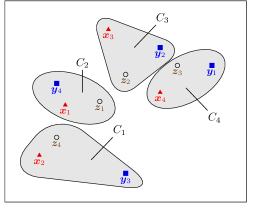
Figure 1: Cliques $C_{i}$ for $\mathcal{A}_{j}=\{X,Y,Z\}$, $k=4$, and permutations $\{\tau_{X^{\prime}}\}_{X^{\prime}\in\mathcal{A}_{j}}=\{\tau_{X},\tau_{Y},\tau_{Z}\}$ with $\tau_{X}(1)=2$, $\tau_{X}(2)=1$, $\tau_{X}(3)=3$, $\tau_{X}(4)=4$; $\tau_{Y}(1)=3$, $\tau_{Y}(2)=4$, $\tau_{Y}(3)=2$, $\tau_{Y}(4)=1$; and $\tau_{Z}(1)=4$, $\tau_{Z}(2)=1$, $\tau_{Z}(3)=2$, $\tau_{Z}(4)=3$. Note that, e.g., $\tau_{Y}(4)=1$ expresses the fact that $\bm{y}_{1}\in C_{4}$.

We define the cost of a clique $C_{i}$ as the sum

$$\sum_{\bm{x}\in C_{i}}\sum_{\bm{x}^{\prime}\in C_{i}}\lVert\bm{x}-\bm{x}^{\prime}\rVert^{2}=\sum_{X\in\mathcal{A}_{j}}\sum_{X^{\prime}\in\mathcal{A}_{j}}\big{\lVert}\bm{x}^{(X)}_{\tau_{X}(i)}-\bm{x}^{(X^{\prime})}_{\tau_{X^{\prime}}(i)}\big{\rVert}^{2}\,.$$ (54)

Finding the collection of cliques $\{C^{*}_{i}\}_{i=1,\dots,k}$ with minimal sum cost, i.e.,

$$\{C^{*}_{i}\}_{i=1,\dots,k}=\operatorname*{arg\,min}_{\{C_{i}\}_{i=1,\dots,k}}\sum_{i=1}^{k}\sum_{\bm{x}\in C_{i}}\sum_{\bm{x}^{\prime}\in C_{i}}\lVert\bm{x}-\bm{x}^{\prime}\rVert^{2}$$ (55)

is then equivalent to finding the optimal collection of permutations in (52). Moreover, according to its definition in (54), the cost of a clique can be decomposed into a sum of squared distances, each between two of its members. Thus, the minimization in (55) is an MDAP with decomposable costs.

Although finding an exact solution to such an MDAP is unfeasible for large $k$ and large clique sizes $\lvert C_{i}\rvert=\lvert\mathcal{A}_{j}\rvert$, there exist various heuristic algorithms producing approximate solutions [37, 38, 39]. Because we are mainly interested in the case of a large clique size, we will merely use a variation of the basic single-hub heuristic and the multi-hub heuristic presented in [37]. Since these heuristic algorithms are used in Step 2 of the proposed LBG-type algorithm, we will label the corresponding steps as 2.1–2.3. The classical single-hub heuristic is based on assigning the vectors $\bm{x}^{(X)}_{i}$ in each point pattern $X\in\mathcal{A}_{j}$ to the $k$ different cliques (using a permutation $\tau_{X}$) by minimizing the sum of squared distances between the vectors $\bm{x}^{(X)}_{\tau(i)}$ and the vectors $\bm{x}^{(X_{1})}_{i}$ of one “hub” point pattern $X_{1}$. More specifically, the algorithm (corresponding to Step 2 of the LBG algorithm) is given as follows.

• Input: a collection $\mathcal{A}_{j}$ of point patterns; each point pattern $X\in\mathcal{A}_{j}$ contains $k$ points in $\mathbb{R}^{d}$.

• Initialization: Choose a point pattern $X_{1}\in\mathcal{A}_{j}$ (called the hub) and define $\tau_{X_{1}}(i)=i$ for $i=1,\dots,k$.

• Step 2.1: For each $X=\big{\{}\bm{x}^{(X)}_{1},\dots,\bm{x}^{(X)}_{k}\big{\}}\in\mathcal{A}_{j}\setminus\{X_{1}\}$, find the best assignment between the vectors in $X$ and $X_{1}$, i.e., a permutation

  $$\tau_{X}=\operatorname*{arg\,min}_{\tau}\sum_{i=1}^{k}\big{\lVert}\bm{x}^{(X)}_{\tau(i)}-\bm{x}^{(X_{1})}_{i}\big{\rVert}^{2}\,.$$ (56)

• Step 2.2: Define the clique $C_{i}$ according to (53), i.e.,

  $$C_{i}\triangleq\big{\{}\bm{x}^{(X)}_{\tau_{X}(i)}:X\in\mathcal{A}_{j}\big{\}},\qquad i=1,\dots,k\,.$$ (57)

• Step 2.3: Define the (approximate) center point pattern $\hat{X}^{*}_{j}$ as the union of the centers (arithmetic means) of all cliques, i.e.,

  $$\hat{X}^{*}_{j}\triangleq\bigcup_{i=1}^{k}\big{\{}\bar{\bm{x}}_{C_{i}}\big{\}}\qquad\text{with }\bar{\bm{x}}_{C_{i}}\triangleq\frac{1}{\lvert C_{i}\rvert}\sum_{\bm{x}\in C_{i}}\bm{x}\,.$$ (58)

• Output: approximate center point pattern $\hat{X}^{*}_{j}$.

The above heuristic requires only $\lvert\mathcal{A}_{j}\rvert-1$ optimal assignments between point patterns. However, the accuracy of the resulting approximate center point pattern $\hat{X}^{*}_{j}$ strongly depends on the choice of the hub $X_{1}$ and can be very poor for certain choices of $X_{1}$. The more robust multi-hub heuristic [37] performs the single-hub algorithm with all the $X\in\mathcal{A}_{j}$ as alternative hubs $X_{1}$, which can be shown to increase the complexity to $\frac{(\lvert\mathcal{A}_{j}\rvert-1)\lvert\mathcal{A}_{j}\rvert}{2}$ optimal assignments, i.e., by a factor of $\lvert\mathcal{A}_{j}\rvert/2$. We here propose a different heuristic that has almost the same complexity as the single-hub heuristic but is more robust. The idea of our approach is to replace the best assignment to the single hub $X_{1}$ by an optimal assignment to the approximate center point pattern of the subsets defined in the preceding steps. More specifically, we start with a hub $X_{1}\in\mathcal{A}_{j}$ and, as in the single-hub heuristic, search for the best assignment $\tau_{X_{2}}$ (see (56) with $X=X_{2}$) between the vectors in a randomly chosen $X_{2}\in\mathcal{A}_{j}\setminus\{X_{1}\}$ and $X_{1}$. Then, we calculate the center point pattern $\hat{X}_{2}$ of $X_{1}$ and $X_{2}$ as in (57) and (58) but with $\mathcal{A}_{j}$ replaced by $\{X_{1},X_{2}\}$. In the next step, we choose a random $X_{3}\in\mathcal{A}_{j}\setminus\{X_{1},X_{2}\}$ and find the optimal assignment $\tau_{X_{3}}$ between the vectors in $X_{3}$ and $\hat{X}_{2}$. An approximate center point pattern $\hat{X}_{3}$ of $X_{1}$, $X_{2}$, and $X_{3}$ is then calculated as in (57) and (58) but with $\mathcal{A}_{j}$ replaced by $\{X_{1},X_{2},X_{3}\}$. Equivalently, we can calculate $\hat{X}_{3}$ as a “weighted” center point pattern of $X_{3}$ and $\hat{X}_{2}$. We proceed in this way with all the point patterns in $\mathcal{A}_{j}$, always calculating the optimal assignment $\tau_{X_{r}}$ ($r=4,5,\dots$) between the vectors in $X_{r}$ and the approximate center point pattern $\hat{X}_{r-1}$ of the previous $r-1$ point patterns. A formal statement of the algorithm is as follows.

• Input: a collection $\mathcal{A}_{j}$ of point patterns; each point pattern $X\in\mathcal{A}_{j}$ contains $k$ points in $\mathbb{R}^{d}$.

• Initialization: (Randomly) order the point patterns $X\in\mathcal{A}_{j}$, i.e., choose a sequence $(X_{1},\dots,X_{\lvert\mathcal{A}_{j}\rvert})$ where the $X_{r}$ are all the elements of $\mathcal{A}_{j}$. Set the initial subset center point pattern $\hat{X}_{1}$ to $X_{1}$.

• For $r=2,\dots,\lvert\mathcal{A}_{j}\rvert$:

  • Step 2.1: Find the best assignment between the vectors in $X_{r}$ and $\hat{X}_{r-1}$, i.e., a permutation $\tau_{X_{r}}=\operatorname*{arg\,min}_{\tau}\sum_{i=1}^{k}\big{\lVert}\bm{x}^{(X_{r})}_{\tau(i)}-\bm{x}^{(\hat{X}_{r-1})}_{i}\big{\rVert}^{2}$.

  • Step 2.2: Generate an updated (approximate) subset center point pattern $\hat{X}_{r}=\big{\{}\bm{x}^{(\hat{X}_{r})}_{1},\dots,\bm{x}^{(\hat{X}_{r})}_{k}\big{\}}$ according to

    $$\bm{x}^{(\hat{X}_{r})}_{i}=\frac{1}{r}\sum_{s=1}^{r}\bm{x}^{(X_{s})}_{\tau_{X_{s}}(i)}=\frac{(r-1)\bm{x}^{(\hat{X}_{r-1})}_{i}+\bm{x}^{(X_{r})}_{\tau_{X_{r}}(i)}}{r}$$ (59)

    for $i=1,\dots,k$.

• Output: approximate center point pattern $\hat{X}^{*}_{j}=\hat{X}_{\lvert\mathcal{A}_{j}\rvert}$.

As in the case of the single-hub heuristic, we only have to perform $\lvert\mathcal{A}_{j}\rvert-1$ optimal assignments. The complexity of the additional center update (59) is negligible. On the other hand, the multi-hub algorithm can be easily parallelized whereas our algorithm works only sequentially.

VI-D Example: Gaussian Distribution

As an example, we consider the case of a PP $\mathsf{X}$ on $\mathbb{R}^{d}$ of fixed cardinality $\lvert\mathsf{X}\rvert=k$ whose points are independently distributed according to a standard Gaussian distribution on $\mathbb{R}^{d}$, i.e., $\bm{\mathsf{x}}_{\mathsf{X}}^{(k)}\in(\mathbb{R}^{d})^{k}$ has i.i.d. zero-mean Gaussian entries with variance $1$. We want to compare the lower bound (43) to the upper bounds presented in Sections VI-B and VI-C and to the RD function for the vector setting, i.e., to the RD function of a standard Gaussian vector $\bm{\mathsf{x}}^{(k)}$ in $(\mathbb{R}^{d})^{k}$. In the PP setting, we use the distortion $\rho_{2}$ (see (42)), while in the vector setting, we use the conventional squared-error distortion. The RD function for $\bm{\mathsf{x}}^{(k)}$ in the vector setting can be calculated in closed form; assuming $D\leq k{d}$, it is equal to

$$R_{\text{vec}}(D)=\frac{k{d}}{{2}}\log\bigg{(}\frac{k{d}}{D}\bigg{)}\,.$$ (60)

This result was shown (see [12, Sec. 10.3.2]) by using the RD theorem for the vector case, i.e., (26) with obvious modifications, and choosing $\bm{\mathsf{x}}^{(k)}=\bm{\mathsf{y}}^{(k)}+\bm{\mathsf{w}}^{(k)}$, where $\bm{\mathsf{w}}^{(k)}$ has i.i.d. zero-mean Gaussian entries with variance $D/(k{d})$, $\bm{\mathsf{y}}^{(k)}$ has i.i.d. zero-mean Gaussian entries with variance $1-D/(k{d})$, and $\bm{\mathsf{y}}^{(k)}$ and $\bm{\mathsf{w}}^{(k)}$ are independent. This choice can be shown to achieve the infimum in the RD theorem and hence the mutual information $I(\bm{\mathsf{x}}^{(k)};\bm{\mathsf{y}}^{(k)})$ is equal to the RD function.

In the PP setting, inserting (60) into (43) results in the lower bound

$$R(D)\geq\frac{kd}{2}\log\bigg{(}\frac{kd}{D}\bigg{)}-\log k!\,.$$ (61)

For the calculation of the upper bound (48), we use a similar approach as in the vector case. Let $\mathsf{X}$ be a PP of fixed cardinality $\lvert\mathsf{X}\rvert=k$, where $\bm{\mathsf{x}}_{\mathsf{X}}^{(k)}$ has i.i.d. zero-mean Gaussian entries with variance $1$. We choose $\bm{\mathsf{x}}^{(k)}=\bm{\mathsf{y}}^{(k)}+\bm{\mathsf{w}}^{(k)}$, where $\bm{\mathsf{w}}^{(k)}$ has i.i.d. zero-mean Gaussian entries with variance $\sigma^{2}<1$, $\bm{\mathsf{y}}^{(k)}$ has i.i.d. zero-mean Gaussian entries with variance $1-\sigma^{2}$, and $\bm{\mathsf{y}}^{(k)}$ and $\bm{\mathsf{w}}^{(k)}$ are independent. The random vectors $\bm{\mathsf{x}}_{\mathsf{X}}^{(k)}$ and $\bm{\mathsf{x}}^{(k)}$ have the same distribution, and the first term on the right-hand side in (48) is here obtained as

$$I\big{(}\bm{\mathsf{x}}^{(k)};\bm{\mathsf{y}}^{(k)}\big{)}=\frac{k{d}}{{2}}\log\bigg{(}\frac{1}{\sigma^{2}}\bigg{)}\,.$$ (62)

The second term on the right-hand side in (48) can be dropped, which in general results in a looser upper bound. However, in our example, this term can be shown to be zero and thus dropping it does not loosen the bound. The third term can be rewritten as

$$- I\big{(}\bm{\mathsf{x}}^{(k)};\mathsf{t}^{(k)}_{\bm{\mathsf{y}}}\,\big{|}\,\phi_{k}(\bm{\mathsf{y}}^{(k)})\big{)}$$

$$=-H\big{(}\mathsf{t}^{(k)}_{\bm{\mathsf{y}}}\,\big{|}\,\phi_{k}(\bm{\mathsf{y}}^{(k)})\big{)}+H\big{(}\mathsf{t}^{(k)}_{\bm{\mathsf{y}}}\,\big{|}\,\phi_{k}(\bm{\mathsf{y}}^{(k)}),\bm{\mathsf{x}}^{(k)}\big{)}\,.$$ (63)

Because all the elements $\bm{\mathsf{y}}^{(k)}_{i}$ of $\bm{\mathsf{y}}^{(k)}$ are i.i.d. and thus symmetric, the associated random permutation $\mathsf{t}^{(k)}_{\bm{\mathsf{y}}}$ is uniformly distributed. Furthermore, this symmetry implies that $\mathsf{t}^{(k)}_{\bm{\mathsf{y}}}$ is independent of the values of the elements of $\phi_{k}(\bm{\mathsf{y}}^{(k)})$. Thus,

$$H\big{(}\mathsf{t}^{(k)}_{\bm{\mathsf{y}}}\,\big{|}\,\phi_{k}(\bm{\mathsf{y}}^{(k)})\big{)}=H\big{(}\mathsf{t}^{(k)}_{\bm{\mathsf{y}}}\big{)}=\log k!\,.$$ (64)

Furthermore, the entropy $H\big{(}\mathsf{t}^{(k)}_{\bm{\mathsf{y}}}\,\big{|}\,\phi_{k}(\bm{\mathsf{y}}^{(k)}),\bm{\mathsf{x}}^{(k)}\big{)}$ is shown in Appendix E to be bounded for any $\varepsilon>0$ according to

$$H \big{(}\mathsf{t}^{(k)}_{\bm{\mathsf{y}}}\,\big{|}\,\phi_{k}(\bm{\mathsf{y}}^{(k)}),\bm{\mathsf{x}}^{(k)}\big{)}$$

$$\leq\bigg{(}\frac{k(k-1)}{2}\,F_{\chi^{2}}\bigg{(}\frac{9\varepsilon^{2}}{2(1-\sigma^{2})};d\bigg{)}+1-F_{\chi^{2}}\bigg{(}\frac{\varepsilon^{2}}{\sigma^{2}};kd\bigg{)}\bigg{)}$$

$$\quad\times\log k!+H_{2}(p_{0}(\varepsilon))+(1-p_{0}(\varepsilon))\log(k!-1)$$ (65)

where $F_{\chi^{2}}(\,\cdot\,;d)$ denotes the cumulative distribution function of a $\chi^{2}$ distribution with $d$ degrees of freedom, $H_{2}(\cdot)$ is the binary entropy function, and $p_{0}(\varepsilon)=1/\big{(}1+(k!-1)\exp\big{(}{-}\frac{3\varepsilon^{2}}{2\sigma^{2}}\big{)}\big{)}$. Inserting (64) and (65) into (63) and, in turn, inserting (62) and (63) into (48), we obtain

$$R(D) \leq\frac{kd}{2}\log\bigg{(}\frac{1}{\sigma^{2}}\bigg{)}-\log k!+\bigg{(}\frac{k(k-1)}{2}$$

$$\quad\times F_{\chi^{2}}\bigg{(}\frac{9\varepsilon^{2}}{2(1-\sigma^{2})};d\bigg{)}+1-F_{\chi^{2}}\bigg{(}\frac{\varepsilon^{2}}{\sigma^{2}};kd\bigg{)}\bigg{)}\log k!$$

$$\quad+H_{2}(p_{0}(\varepsilon))+(1-p_{0}(\varepsilon))\log(k!-1)$$ (66)

provided that (47) is satisfied. Due to (49), this is the case if $\mathbb{E}\big{[}\lVert\bm{\mathsf{x}}^{(k)}-\bm{\mathsf{y}}^{(k)}\rVert^{2}\big{]}\leq D$. Because $\mathbb{E}\big{[}\lVert\bm{\mathsf{x}}^{(k)}-\bm{\mathsf{y}}^{(k)}\rVert^{2}\big{]}=\mathbb{E}\big{[}\lVert\bm{\mathsf{w}}^{(k)}\rVert^{2}\big{]}=dk\sigma^{2}$, we thus choose $\sigma^{2}=D/(kd)$.

By choosing $\varepsilon$ appropriately, we can show that the upper bound (66) converges to the lower bound (61) as $D\to 0$, i.e., that the lower bound (61) is asymptotically tight. Indeed, choosing $\varepsilon>0$ such that $\varepsilon\to 0$ and $\varepsilon/\sigma\to\infty$ as $D\to 0$, we obtain $F_{\chi^{2}}\big{(}\frac{9\varepsilon^{2}}{2(1-\sigma^{2})};d\big{)}\to 0$, $F_{\chi^{2}}\big{(}\frac{\varepsilon^{2}}{\sigma^{2}};kd\big{)}\to 1$, and $p_{0}(\varepsilon)\to 1$. Thus, (66) gives

$$R(D)\leq\frac{kd}{2}\log\bigg{(}\frac{kd}{D}\bigg{)}-\log k!+o(1)$$ (67)

where $o(1)$ is a function that converges to zero as $D\to 0$.

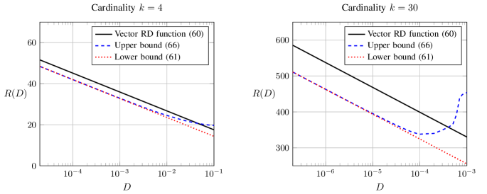
Figure 2: Lower bound on the RD function according to (61) and upper bound on the RD function according to (66) with $\varepsilon=\sigma^{3/4}=(D/(kd))^{3/8}$ for a PP of fixed cardinality $k$ (left: $k=4$; right: $k=30$) and with $\bm{\mathsf{x}}_{\mathsf{X}}^{(k)}$ following a multivariate standard normal distribution. For comparison, also the corresponding vector RD function (60) is shown.

In Figure 2, we show the upper bound (66) for $d=2$, cardinalities $k=4$ and $k=30$, and $\varepsilon=\sigma^{3/4}=(D/(kd))^{3/8}$ in comparison to the lower bound (61) and the vector RD function (60). We see that as $D\to 0$, our upper and lower bounds are tight. However, as the upper bound was designed for small values of $D$, it is not useful for larger values of $D$.

We also considered codebook-based upper bounds following (40). Using the LBG-type algorithm presented in Sections V-B and VI-C, we constructed codebooks for fixed-cardinality PPs with $k=4$ and $k=30$ i.i.d. Gaussian points. As input to the LBG algorithm, we used $\lvert\mathcal{A}\rvert=100\cdot M$ random realizations of the source PP. In Step 2 of the algorithm, we employed the multi-hub heuristic as well as the modified single-hub heuristic proposed in Section VI-C. The expected distortion $\widetilde{D}=\mathbb{E}[\rho_{2}(\mathsf{X},g(\mathsf{X}))]$ for each constructed source code $g$ was calculated using Monte Carlo integration [40, Ch. 3]. In Figure 3, we show the resulting upper bounds on the RD function based on codebooks of up to $M=2048$ codewords in comparison to the lower bound (61) and the vector RD function (60). Unfortunately, for larger values of $M$, Step 1 in the LBG algorithm becomes computationally unfeasible. It can be seen that the PP setting can significantly reduce the required rates compared to the vector setting also for large values of $D$. Furthermore, using the significantly less computationally demanding modified single-hub heuristic does not result in increased upper bounds compared to the multi-hub heuristic.

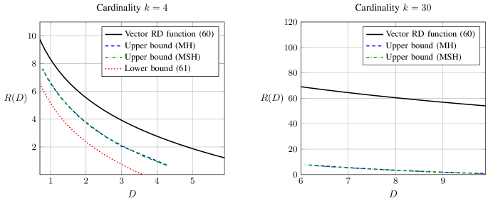
Figure 3: Numerical codebook-based upper bounds on the RD function of a PP of fixed cardinality $k$ (left: $k=4$; right: $k=30$) and with $\bm{\mathsf{x}}_{\mathsf{X}}^{(k)}$ following a multivariate standard normal distribution. The codebook construction underlying the upper bounds used the multi-hub heuristic (MH) or the proposed modified single-hub heuristic (MSH). For comparison, also the corresponding vector RD function (60) and the lower bound (61) are shown. (The latter is shown only for $k=4$, because for $k=30$ it is below $0$ in the regime where code construction is feasible.)

VII Poisson Point Processes

Poisson PPs, the most prominent and widely used class of PPs, are characterized by a complete randomness property. A PP $\mathsf{X}$ on $\mathbb{R}^{d}$ is a Poisson PP if the number of points in each Borel set $A\subseteq\mathbb{R}^{d}$ is Poisson distributed with parameter $\lambda(A)$—where the measure $\lambda$ is referred to as the intensity measure of $\mathsf{X}$—and for any disjoint Borel sets $A,B\subseteq\mathbb{R}^{d}$, the number of points in $A$ is independent of the number of points in $B$. For a formal definition see [2, Sec. 2.4]. We will assume that $\mathsf{X}$ is a finite Poisson PP, which satisfies $\lambda(\mathbb{R}^{d})<\infty$. In this setting, we easily obtain the cardinality distribution $p_{\lvert\mathsf{X}\rvert}$ and the measures $P_{\mathsf{X}}^{(k)}$. Let us express the intensity measure as $\lambda=\nu\lambda_{0}$, where $\nu\triangleq\lambda(\mathbb{R}^{d})\in\mathbb{R}_{\geq 0}$ and $\lambda_{0}\triangleq\lambda/\nu$ is a probability measure. We then obtain

$$p_{\lvert\mathsf{X}\rvert}(k)=\frac{e^{-\nu}\nu^{k}}{k!}\qquad\text{ for }k\in\mathbb{N}_{0}$$ (68)

and moreover it can be shown that (see [2, Sec. 5.3])

$$P_{\mathsf{X}}^{(k)}=\lambda_{0}^{k}\qquad\text{ for }k\in\mathbb{N}\,.$$ (69)

Note that (69) implies that for a given cardinality $\lvert\mathsf{X}\rvert=k$, the vectors $\bm{\mathsf{x}}_{i}\in\mathsf{X}$ are i.i.d. with probability measure $\lambda_{0}$.

In the following, we will often consider Poisson PPs with intensity measure $\lambda=\nu\lambda_{0}$, where $\lambda_{0}$ is absolutely continuous with respect to $\mathscr{L}^{d}$ with Radon-Nikodym derivative $g_{\mathsf{X}}=\frac{\mathrm{d}\lambda_{0}}{\mathrm{d}\mathscr{L}^{d}}$. According to (69), this implies that the probability measures $P_{\mathsf{X}}^{(k)}$ are absolutely continuous with respect to $(\mathscr{L}^{d})^{k}$ with Radon-Nikodym derivative

$$\frac{\mathrm{d}P_{\mathsf{X}}^{(k)}}{\mathrm{d}(\mathscr{L}^{d})^{k}}(\bm{x}_{1:k})=f^{(k)}_{\mathsf{X}}(\bm{x}_{1:k})=\prod_{i=1}^{k}g_{\mathsf{X}}(\bm{x}_{i})$$ (70)

i.e., the $\bm{\mathsf{x}}_{\mathsf{X}}^{(k)}$ are continuous random vectors with probability density function $\prod_{i=1}^{k}g_{\mathsf{X}}(\bm{x}_{i})$.

VII-A Distortion Function

For a Poisson PP $\mathsf{X}$, there is a nonzero probability that $\lvert\mathsf{X}\rvert=k$ for each $k\in\mathbb{N}_{0}$. Thus, for an RD analysis, we have to define a distortion function between point patterns of different cardinalities. We choose the squared OSPA distance [25] (up to a normalization factor). For $X=\{\bm{x}_{1},\dots,\bm{x}_{k}\}$ and $Y=\{\bm{y}_{1},\dots,\bm{y}_{\ell}\}$ with $k\leq\ell$, we define the unnormalized squared OSPA (USOSPA) distortion

$$\rho_{2}^{(c)}(X,Y)\triangleq(\ell-k)\,c^{2}+\min_{\tau}\sum_{i=1}^{k}\min\big{\{}\lVert\bm{x}_{i}-\bm{y}_{\tau(i)}\rVert^{2},c^{2}\big{\}}$$

where $c>0$ is a parameter (the cut-off value) and the outer minimum is taken over all permutations $\tau$ on $\{1,\dots,\ell\}$. For $k>\ell$, we define $\rho_{2}^{(c)}(X,Y)\triangleq\rho_{2}^{(c)}(Y,X)$. According to (LABEL:eq:ospagen), the USOSPA distortion is constructed by first penalizing the difference in cardinalities via the term $\lvert\ell-k\rvert\,c^{2}$. Then an optimal assignment between the points of $X$ and $Y$ is established based on the Euclidean distance, and the minima of the squared distances and $c^{2}$ are summed. To bound the RD function, we will use the following bounds on the USOSPA distortion, which are proved in Appendix F.

Lemma 17:

Let $X=\{\bm{x}_{1},\dots,\bm{x}_{k}\}\in\mathcal{N}$ and $Y=\{\bm{y}_{1},\dots,\bm{y}_{\ell}\}\in\mathcal{N}$. Then for $k\geq\ell$

$$\rho_{2}^{(c)}(X,Y)\geq\sum_{i=1}^{k}\min_{j=1}^{\ell}\min\{\lVert\bm{x}_{i}-\bm{y}_{j}\rVert^{2},c^{2}\}$$ (72)

and for $k\leq\ell$

$$\rho_{2}^{(c)}(X,Y)\geq(\ell-k)c^{2}+\sum_{i=1}^{k}\min_{j=1}^{\ell}\min\{\lVert\bm{x}_{i}-\bm{y}_{j}\rVert^{2},c^{2}\}\,.$$ (73)

VII-B Lower Bounds for Poisson Point Processes

Based on Theorem 11 and Lemma 17, we can formulate lower bounds on the RD function of Poisson PPs. A proof of the following result is given in Appendix G.

Theorem 18:

Let $\mathsf{X}$ be a Poisson PP on $\mathbb{R}^{d}$ with intensity measure $\lambda=\nu\lambda_{0}$, where $\lambda_{0}$ is absolutely continuous with respect to $\mathscr{L}^{d}$ with probability density function $g_{\mathsf{X}}=\frac{\mathrm{d}\lambda_{0}}{\mathrm{d}\mathscr{L}^{d}}$. Furthermore, let $A$ be a Borel set satisfying $\int_{A}g_{\mathsf{X}}(\bm{x})\,\mathrm{d}\bm{x}=1$, i.e., $g_{\mathsf{X}}(\bm{x})=0$ for $\mathscr{L}^{d}$-almost all $\bm{x}\in A^{c}$. Then the RD function of $\mathsf{X}$ using distortion $\rho_{2}^{(c)}$ is lower-bounded as

$$R(D) \geq\nu\,h(g_{\mathsf{X}})+\max_{s\geq 1/c^{2}}\bigg{(}{-}\sum_{k\in\mathbb{N}}\frac{e^{-\nu}\nu^{k}}{k!}$$

$$\quad\times\log\big{(}\min\big{\{}(\mathscr{L}^{d}(A))^{k},\widetilde{\gamma}_{k}(s)\big{\}}\big{)}-sD\bigg{)}$$ (74)

where

$$\widetilde{\gamma}_{k}(s) \triangleq\Bigg{(}e^{-sc^{2}}\mathscr{L}^{d}(A)$$

$$\quad+k\bigg{(}{-}e^{-sc^{2}}\mathscr{L}^{d}(U_{c})+\int_{U_{c}}e^{-s\lVert\bm{x}\rVert^{2}}\mathrm{d}\bm{x}\bigg{)}\Bigg{)}^{k}$$ (75)

with $U_{c}\triangleq\{\bm{x}\in\mathbb{R}^{d}:\lVert\bm{x}\rVert\leq c\}$.

Note that the PP $\mathsf{X}$ enters the bound (74) only via $\nu$ and the differential entropy $h(g_{\mathsf{X}})$. In particular, the functions $\widetilde{\gamma}_{k}$ in (75) do not depend on $\mathsf{X}$. However, they do depend on the set $A$.

Example 19:

Let $\mathsf{X}$ be a Poisson PP on $\mathbb{R}^{2}$ with intensity measure $\lambda=\nu\mathscr{L}^{2}|_{[0,1)^{2}}$, i.e., the points are independently and uniformly distributed on the unit square. In this setting, we have $g_{\mathsf{X}}=\mathbbm{1}_{[0,1)^{2}}$ and we can choose $A=[0,1)^{2}$ in Theorem 18. The differential entropy $h(g_{\mathsf{X}})$ is zero, because the density $g_{\mathsf{X}}=\mathbbm{1}_{[0,1)^{2}}$ takes on the values zero or one. Furthermore, we have $d=2$, and thus, using $\mathscr{L}^{2}(A)=1$, $\mathscr{L}^{2}(U_{c})=\pi c^{2}$, and $\int_{U_{c}}e^{-s\lVert\bm{x}\rVert^{2}}\mathrm{d}\bm{x}=\frac{\pi}{s}\big{(}1-e^{-sc^{2}}\big{)}$, (75) reduces to

$$\widetilde{\gamma}_{k}(s)=\Bigg{(}e^{-sc^{2}}\bigg{(}1-\pi c^{2}k-\frac{\pi k}{s}\bigg{)}+\frac{\pi k}{s}\Bigg{)}^{k}.$$

We further obtain

$$\log\big{(}\min\big{\{}(\mathscr{L}^{2}(A))^{k},\widetilde{\gamma}_{k}(s)\big{\}}\big{)}$$

$$\quad=\min\big{\{}k\log\mathscr{L}^{2}(A),\log\widetilde{\gamma}_{k}(s)\big{\}}$$

$$\quad=\min\{0,\log\widetilde{\gamma}_{k}(s)\}$$

i.e., we can upper-bound $\log\big{(}\min\big{\{}(\mathscr{L}^{2}(A))^{k},\widetilde{\gamma}_{k}(s)\big{\}}\big{)}$ either by zero (which corresponds to omitting the $k$th summand in (74)) or by $\log\widetilde{\gamma}_{k}(s)$. In particular, we can omit all but the first $k_{\text{max}}\in\mathbb{N}_{0}$ summands in the lower bound (74) and, in the remaining summands, bound the factors $\log\big{(}\min\big{\{}(\mathscr{L}^{2}(A))^{k},\widetilde{\gamma}_{k}(s)\big{\}}\big{)}$ by $\log\widetilde{\gamma}_{k}(s)$. We then obtain

$$R(D) \geq\max_{s\geq 1/c^{2}}\bigg{(}{-}\sum_{k=1}^{k_{\text{max}}}\frac{e^{-\nu}\nu^{k}}{k!}\log\widetilde{\gamma}_{k}(s)-sD\bigg{)}$$

$$=\max_{s\geq 1/c^{2}}\bigg{(}{-}\sum_{k=1}^{k_{\text{max}}}\frac{e^{-\nu}\nu^{k}}{(k-1)!}$$

$$\quad\times\log\bigg{(}e^{-sc^{2}}\bigg{(}1-\pi c^{2}k-\frac{\pi k}{s}\bigg{)}+\frac{\pi k}{s}\bigg{)}-sD\bigg{)}$$ (76)

where we used $h(g_{\mathsf{X}})=0$.

Let us next investigate the convexity properties of the right-hand side in (76). The second derivative of $\log\widetilde{\gamma}_{k}(s)$ is obtained as

$$(\log\widetilde{\gamma}_{k}(s))^{\prime\prime}$$

$$\quad=\!\Big{(}\pi k^{2}\big{(}(1-\pi c^{2}k)({c}^{4}{s}^{3}-{c}^{2}{s}^{2}-2s{e^{-s{c}^{2}}}+2s)$$

$$\quad\quad-{c}^{2}{s}^{2}+e^{-s{c}^{2}}\pi k(1-e^{sc^{2}})^{2}\big{)}\Big{)}$$

$$\quad\quad\times{s}^{-2}e^{s{c}^{2}}\big{(}\pi{c}^{2}ks+\pi k-\pi ke^{s{c}^{2}}-s\big{)}^{-2}\,.$$ (77)

It can be shown that $(\log\widetilde{\gamma}_{k}(s))^{\prime\prime}>0$ if $s\geq 3/c^{2}$ and $k\leq 1/(2\pi c^{2})$. Hence, $\log\widetilde{\gamma}_{k}$ is convex in that case. In particular, choosing $k_{\text{max}}\leq 1/(2\pi c^{2})$, we have that $\log\widetilde{\gamma}_{k}$ is a convex function for $k\leq k_{\text{max}}$ and $s\geq 3/c^{2}$, and thus the sum on the right-hand side in (76) is—as a sum of concave functions—concave. Hence, if we restrict the maximization in (76) to $s\geq 3/c^{2}$, we obtain a lower bound for given values of $c$, $k_{\text{max}}\leq 1/(2\pi c^{2})$, $\nu$, and $D$ that we can compute using standard numerical algorithms. In Figure 4, we show this lower bound for $c=0.1$, $k_{\text{max}}=\lfloor 1/(2\pi c^{2})\rfloor=15$, $\nu=10$, and various values of $D$.

For $k_{\text{max}}>1/(2\pi c^{2})$, the right-hand side in (76) is not guaranteed to be concave. However, we can still use numerical solvers to try to find local maxima of (76) that give even better results. In particular, we show in Figure 4 also an optimized lower bound for $k_{\text{max}}=50$.

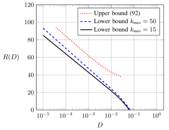
Figure 4: Lower and upper bounds on the RD function for a Poisson PP with uniform intensity measure $\lambda=10\cdot\mathscr{L}^{2}|_{[0,1)^{2}}$ on $[0,1)^{2}$, using the USOSPA distortion with cut-off value $c=0.1$.

VII-C Upper Bound for Poisson Point Processes

Next, we establish an upper bound on the RD function of a Poisson PP $\mathsf{X}$. In the following theorem, which is proven in Appendix H, we apply Corollary 12 to vectors $(\bm{\mathsf{x}}^{(k)},\bm{\mathsf{y}}^{(k)})$ where $\bm{\mathsf{x}}^{(k)}$ has the same distribution as $\bm{\mathsf{x}}_{\mathsf{X}}^{(k)}$.

Theorem 20:

Let $\mathsf{X}$ be a Poisson PP on $\mathbb{R}^{d}$ with intensity measure $\lambda=\nu\lambda_{0}$, where $\lambda_{0}$ is absolutely continuous with respect to $\mathscr{L}^{d}$ with probability density function $g_{\mathsf{X}}=\frac{\mathrm{d}\lambda_{0}}{\mathrm{d}\mathscr{L}^{d}}$. Furthermore, let $\lambda_{\mathsf{Y}}$ be a probability measure on $\mathbb{R}^{d}$ and let $\bm{\mathsf{y}}^{(k)}$ be random vectors on $(\mathbb{R}^{d})^{k}$ with probability measure $(\lambda_{\mathsf{Y}})^{k}$ for each $k\in\mathbb{N}$. Define the joint distribution of $(\bm{\mathsf{x}}^{(k)},\bm{\mathsf{y}}^{(k)})$ by a given conditional probability density function $g_{\bm{\mathsf{x}}^{(k)}\mid\bm{\mathsf{y}}^{(k)}}(\bm{x}_{1:k}\,|\,\bm{y}_{1:k})$ on $(\mathbb{R}^{d})^{k}$ for each $\bm{y}_{1:k}\in(\mathbb{R}^{d})^{k}$. Assume that the resulting random vector $\bm{\mathsf{x}}^{(k)}$ has the same distribution as $\bm{\mathsf{x}}_{\mathsf{X}}^{(k)}$ (see (70)), i.e.,

$$\prod_{i=1}^{k}g_{\mathsf{X}}(\bm{x}_{i})=\int_{(\mathbb{R}^{d})^{k}}g_{\bm{\mathsf{x}}^{(k)}\mid\bm{\mathsf{y}}^{(k)}}(\bm{x}_{1:k}\,|\,\bm{y}_{1:k})\,\mathrm{d}\lambda_{\mathsf{Y}}^{k}(\bm{y}_{1:k})$$ (78)

and that

$$\sum_{k\in\mathbb{N}}\frac{e^{-\nu}\nu^{k}}{k!}\,\mathbb{E}\big{[}\rho_{2}^{(c)}\big{(}\phi_{k}(\bm{\mathsf{x}}^{(k)}),\phi_{k}(\bm{\mathsf{y}}^{(k)})\big{)}\big{]}\leq D$$ (79)

where

$$\mathbb{E}\big{[}\rho_{2}^{(c)}\big{(}\phi_{k}(\bm{\mathsf{x}}^{(k)}),\phi_{k}(\bm{\mathsf{y}}^{(k)})\big{)}\big{]}$$

$$\rule{28.45274pt}{0.0pt}=\int_{(\mathbb{R}^{d})^{k}}\int_{(\mathbb{R}^{d})^{k}}\rho_{2}^{(c)}(\phi_{k}(\bm{x}_{1:k}),\phi_{k}(\bm{y}_{1:k}))\,$$

$$\rule{28.45274pt}{0.0pt}\quad\times g_{\bm{\mathsf{x}}^{(k)}\mid\bm{\mathsf{y}}^{(k)}}(\bm{x}_{1:k}\,|\,\bm{y}_{1:k})\,\mathrm{d}\lambda_{\mathsf{Y}}^{k}(\bm{y}_{1:k})\,\mathrm{d}\bm{x}_{1:k}\,.$$

Then

$$R(D) \leq\nu-\nu\log\nu+\nu\,h(g_{\mathsf{X}})$$

$$\quad+\sum_{k\in\mathbb{N}}\frac{e^{-\nu}\nu^{k}}{k!}\big{(}\log k!-h\big{(}\bm{\mathsf{x}}^{(k)}\,\big{|}\,\bm{\mathsf{y}}^{(k)}\big{)}\big{)}$$ (80)

where

$$h\big{(}\bm{\mathsf{x}}^{(k)}\,\big{|}\,\bm{\mathsf{y}}^{(k)}\big{)}=\int_{(\mathbb{R}^{d})^{k}}h\big{(}\bm{\mathsf{x}}^{(k)}\,\big{|}\,\bm{\mathsf{y}}^{(k)}=\bm{y}_{1:k}\big{)}\,\mathrm{d}\lambda_{\mathsf{Y}}^{k}(\bm{y}_{1:k})$$ (81)

with

$$h\big{(}\bm{\mathsf{x}}^{(k)}\,\big{|}\,\bm{\mathsf{y}}^{(k)}=\bm{y}_{1:k}\big{)} =-\int_{(\mathbb{R}^{d})^{k}}g_{\bm{\mathsf{x}}^{(k)}\mid\bm{\mathsf{y}}^{(k)}}(\bm{x}_{1:k}\,|\,\bm{y}_{1:k})$$

$$\quad\times\log g_{\bm{\mathsf{x}}^{(k)}\mid\bm{\mathsf{y}}^{(k)}}(\bm{x}_{1:k}\,|\,\bm{y}_{1:k})\,\mathrm{d}\bm{x}_{1:k}\,.$$ (82)

In the proof of Theorem 20 in Appendix H, we do not make use of the conditional mutual informations in (37). Although this loosens the bound in general, it does not if we use a conditional probability density function $g_{\bm{\mathsf{x}}^{(k)}\mid\bm{\mathsf{y}}^{(k)}}(\bm{x}_{1:k}\,|\,\bm{y}_{1:k})$ that does not depend on the ordering of the elements $\bm{y}_{1},\dots,\bm{y}_{k}$. Indeed, this additional assumption can be shown to imply that the conditional mutual informations in (37) are zero and thus can be dropped without loosening the bound. This is in stark contrast to the setting we encountered in Section VI-D, where the conditional mutual informations are required to obtain a useful upper bound. Indeed, these two settings illustrate different proof strategies: Either the joint distribution of $\bm{\mathsf{x}}^{(k)}$ and $\bm{\mathsf{y}}^{(k)}$ is carefully constructed to gain conditional independence of the orderings, or we have to analyze the conditional mutual informations in (37) in detail. Next, we use Theorem 20 with such a carefully constructed conditional probability density function to obtain upper bounds on the RD function of the Poisson PP discussed in Example 19.

Example 21:

Let $\mathsf{X}$ be a Poisson PP on $\mathbb{R}^{2}$ with intensity measure $\lambda=\nu\mathscr{L}^{2}|_{[0,1)^{2}}$, i.e., $g_{\mathsf{X}}=\mathbbm{1}_{[0,1)^{2}}$. To use Theorem 20, we have to define a measure $\lambda_{\mathsf{Y}}$ and conditional probability density functions $g_{\bm{\mathsf{x}}^{(k)}\mid\bm{\mathsf{y}}^{(k)}}(\bm{x}_{1:k}\,|\,\bm{y}_{1:k})$ such that (78) is satified, i.e., in our case,

$$\int_{(\mathbb{R}^{2})^{k}}g_{\bm{\mathsf{x}}^{(k)}\mid\bm{\mathsf{y}}^{(k)}}(\bm{x}_{1:k}\,|\,\bm{y}_{1:k})\,\mathrm{d}\lambda_{\mathsf{Y}}^{k}(\bm{y}_{1:k})=\prod_{i=1}^{k}\mathbbm{1}_{[0,1)^{2}}(\bm{x}_{i})\,.$$ (83)

To this end, for $N\in\mathbb{N}$ satisfying $N\geq 1/(\sqrt{2}c)$ (this condition will be used later), we define $\lambda_{\mathsf{Y}}$ as

$$\lambda_{\mathsf{Y}}(C)=\frac{1}{N^{2}}\sum_{j_{1}=1}^{N}\sum_{j_{2}=1}^{N}\delta_{\bm{q}_{j_{1},j_{2}}}(C)$$ (84)

for $C\in\mathcal{B}_{2}$, where $\delta_{\bm{x}}$ denotes the point measure at $\bm{x}$ and $\bm{q}_{j_{1},j_{2}}=\big{(}\frac{2j_{1}-1}{2N},\frac{2j_{2}-1}{2N}\big{)}$. Hence, $\lambda_{\mathsf{Y}}$ corresponds to a discrete uniform distribution with the $N^{2}$ possible realizations $\bm{q}_{j_{1},j_{2}}$, $j_{1},j_{2}\in\{1,\dots,N\}$. Furthermore, consider a set of $k$ index pairs $\big{\{}\big{(}j_{1}^{(i)},j_{2}^{(i)}\big{)}\big{\}}_{i=1,\dots,k}\subseteq\{1,\dots,N\}^{2}$. The function $g_{\bm{\mathsf{x}}^{(k)}\mid\bm{\mathsf{y}}^{(k)}}(\bm{x}_{1:k}\,|\,\bm{y}_{1:k})$ is then defined for $\bm{y}_{i}=\bm{q}_{j_{1}^{(i)},j_{2}^{(i)}}$ by

$$g_{\bm{\mathsf{x}}^{(k)}\mid\bm{\mathsf{y}}^{(k)}}\big{(}\bm{x}_{1:k} \,\big{|}\,\big{(}\bm{q}_{j_{1}^{(1)},j_{2}^{(1)}},\dots,\bm{q}_{j_{1}^{(k)},j_{2}^{(k)}}\big{)}\big{)}$$

$$=\frac{1}{k!}\sum_{\tau}\prod_{i=1}^{k}N^{2}\mathbbm{1}_{Q_{j_{1}^{(\tau(i))},j_{2}^{(\tau(i))}}}(\bm{x}_{i})$$ (85)

$$=\frac{N^{2k}}{k!}\sum_{\tau}\mathbbm{1}_{\prod_{i=1}^{k}Q_{j_{1}^{(\tau(i))},j_{2}^{(\tau(i))}}}(\bm{x}_{1:k})$$ (86)

where $Q_{j_{1},j_{2}}\triangleq\big{[}{-}\frac{1}{2N},\frac{1}{2N}\big{)}^{2}+\bm{q}_{j_{1},j_{2}}$ and the sum is over all permutations $\tau$ on $\{1,\dots,k\}$. Note that $\{Q_{j_{1},j_{2}}\}_{j_{1},j_{2}=1,\dots,N}$ constitutes a partition of $[0,1)^{2}$ into $N^{2}$ squares. Furthermore, note that $N^{2}\mathbbm{1}_{Q_{j_{1}^{(\tau(i))},j_{2}^{(\tau(i))}}}$ is the probability density function of a uniform random vector on the square $Q_{j_{1}^{(\tau(i))},j_{2}^{(\tau(i))}}$. Thus, the distribution specified by (85) can be interpreted as first randomly choosing an assignment (represented by $\tau$) between $\{\bm{\mathsf{x}}_{i}\}_{i=1,\dots,k}$ and $\big{\{}\bm{q}_{j_{1}^{(i)},j_{2}^{(i)}}\big{\}}_{i=1,\dots,k}$, and then distributing $\bm{\mathsf{x}}_{i}$ uniformly and independently on the square $Q_{j_{1}^{(\tau(i))},j_{2}^{(\tau(i))}}$ with center $\bm{q}_{j_{1}^{(\tau(i))},j_{2}^{(\tau(i))}}$. In particular, $g_{\bm{\mathsf{x}}^{(k)}\mid\bm{\mathsf{y}}^{(k)}}\big{(}\bm{x}_{1:k}\,\big{|}\,\big{(}\bm{q}_{j_{1}^{(1)},j_{2}^{(1)}},\dots,\allowbreak\bm{q}_{j_{1}^{(k)},j_{2}^{(k)}}\big{)}\big{)}$ does not depend on the ordering of the points $\bm{q}_{j_{1}^{(1)},j_{2}^{(1)}},\allowbreak\dots,\allowbreak\bm{q}_{j_{1}^{(k)},j_{2}^{(k)}}$.

By Lemma 27 in Appendix I, $\lambda_{\mathsf{Y}}$ defined by (84) and $g_{\bm{\mathsf{x}}^{(k)}\mid\bm{\mathsf{y}}^{(k)}}$ defined by (85) satisfy (83). Furthermore, by Lemma 28 in Appendix I, the left-hand side of (79) is given as

$$\sum_{k\in\mathbb{N}}\frac{e^{-\nu}\nu^{k}}{k!}\,\mathbb{E}\big{[}\rho_{2}^{(c)}\big{(}\phi_{k}(\bm{\mathsf{x}}^{(k)}),\phi_{k}(\bm{\mathsf{y}}^{(k)})\big{)}\big{]}=\frac{\nu}{6N^{2}}\,.$$ (87)

Thus, condition (79) is satisfied for $D\geq\nu/(6N^{2})$ and, in particular, for $D=\nu/(6N^{2})$.

Finally, we will simplify the bound (80) for our setting. We first recall that the differential entropy $h(g_{\mathsf{X}})$ is zero (see Example 19). Furthermore, according to Lemma 29 in Appendix I, the conditional differential entropy $h\big{(}\bm{\mathsf{x}}^{(k)}\,\big{|}\,\bm{\mathsf{y}}^{(k)}\big{)}$ can be lower-bounded by

$$h\big{(}\bm{\mathsf{x}}^{(k)}\,\big{|}\,\bm{\mathsf{y}}^{(k)}\big{)} \geq\frac{\binom{N^{2}}{k}k!}{N^{2k}}\log k!-k\log N^{2}\,.$$ (88)

Inserting $D=\nu/(6N^{2})$, $h(g_{\mathsf{X}})=0$, and (88) into (80), we obtain

$$R\bigg{(}\frac{\nu}{6N^{2}}\bigg{)} \leq\nu-\nu\log\nu+\sum_{k\in\mathbb{N}}\frac{e^{-\nu}\nu^{k}}{k!}\big{(}\log k!+k\log N^{2}\big{)}$$

$$\quad-\sum_{k=1}^{N^{2}}\frac{e^{-\nu}\nu^{k}\binom{N^{2}}{k}}{N^{2k}}\log k!$$ (89)

where we used that $\binom{N^{2}}{k}=0$ for $k>N^{2}$. By Lemma 30 in Appendix I with $\widetilde{N}=N$, (89) implies

$$R\bigg{(}\frac{\nu}{6N^{2}}\bigg{)} \leq\nu+\nu\log\frac{N^{2}}{\nu}+\sum_{k=1}^{N^{2}}e^{-\nu}\nu^{k}\log k!\bigg{(}\frac{1}{k!}-\frac{\binom{N^{2}}{k}}{N^{2k}}\bigg{)}$$

$$\quad+\bigg{(}1-\sum_{k=0}^{N^{2}-2}\frac{e^{-\nu}\nu^{k}}{k!}\bigg{)}\nu^{2}\,.$$ (90)

The bound (21) can be calculated explicitly for various $N$. However, for large $N$, this is computationally intensive. The computational complexity can be reduced by omitting the summands with $k>N_{\max}^{2}$, where $N_{\max}\leq N$, in the last sum in (89), which results in

$$R\bigg{(}\frac{\nu}{6N^{2}}\bigg{)} \leq\nu-\nu\log\nu+\sum_{k\in\mathbb{N}}\frac{e^{-\nu}\nu^{k}}{k!}\big{(}\log k!+k\log N^{2}\big{)}$$

$$\quad-\sum_{k=1}^{N_{\max}^{2}}\frac{e^{-\nu}\nu^{k}\binom{N^{2}}{k}}{N^{2k}}\log k!\,.$$ (91)

Again using Lemma 30 in Appendix I, this time with $\widetilde{N}=N_{\max}$, we finally obtain

$$R\bigg{(}\frac{\nu}{6N^{2}}\bigg{)} \leq\nu+\nu\log\frac{N^{2}}{\nu}+\sum_{k=1}^{N_{\max}^{2}}e^{-\nu}\nu^{k}\log k!\bigg{(}\frac{1}{k!}-\frac{\binom{N^{2}}{k}}{N^{2k}}\bigg{)}$$

$$\quad+\bigg{(}1-\sum_{k=0}^{N_{\max}^{2}-2}\frac{e^{-\nu}\nu^{k}}{k!}\bigg{)}\nu^{2}\,.$$ (92)

In Figure 4, this upper bound is depicted for the case $\nu=10$, $c=0.1$, $N_{\max}=\min\{N,10\}$, and $N$ ranging from $8$ to $207$ (corresponding to $D=\nu/(6N^{2})$ ranging from $3.9\cdot 10^{-5}$ to $2.6\cdot 10^{-2}$).

VIII Conclusion

We established lower and upper bounds on the RD function of finite PPs. Our bounds provide insights into the behavior of the RD function and demonstrate that the RD function based on the PP viewpoint can be significantly lower than the RD function based on the vector viewpoint. Furthermore, the PP viewpoint allows sets of different sizes to be considered in a single source coding scenario. Our lower bounds are based on the general RD characterization in [28]. Our upper bounds are based either on the RD theorem and an expression of the mutual information between PPs or on a concrete source code.

To enable a comparison with the vector viewpoint, we considered PPs of fixed cardinality with a specific distortion function. For consistency with the classical squared-error distortion, we used a squared-error distortion between optimally assigned point patterns. To obtain upper bounds, we established a relation between the mutual informations for random vectors and for PPs. We further proposed a Lloyd-type algorithm for the construction of source codes. We applied our upper bounds to a PP of fixed cardinality where all points are Gaussian and i.i.d. The result implies that the RD function in the PP setting is significantly smaller than that of a Gaussian vector of the same dimension. Furthermore, we showed that our upper bound converges to the lower bound as the distortion goes to zero.

The complexity of our proposed Lloyd-type algorithm does not scale well in the codebook size and the cardinality of the point patterns. An efficient heuristic scheme for computing the “center point pattern” for a large collection of point patterns would significantly reduce the complexity but does not seem to be available. We note that our algorithm can be easily generalized to PPs of variable cardinality by sorting the collection of point patterns representing the source according to their cardinality and then performing the algorithm for each cardinality separately. However, an algorithm that is able to find center point patterns directly for point patterns of different cardinality may result in better source codes. A first approach in this direction was presented in [41]. Another possible extension of our codebook construction is to encode several successive point patterns jointly, resulting in a source code of length greater than one. This is expected to yield tighter upper bounds, but also to result in a higher computational complexity.

As an example of PPs with variable cardinality, we studied Poisson PPs along with an unnormalized squared OSPA distortion function. For a Poisson PP of uniform intensity on the unit square in $\mathbb{R}^{2}$, our lower and upper bounds are separated by only a small gap and thus provide a good characterization of the RD function. For the construction of the upper bound, we used a uniform quantization. This quantization can also be employed to construct source codes and is a first, simple constructive approach to the generation of source codes for PPs. We expect that—similar to the vector case—finding a good systematic source code construction for general PPs is challenging.

The specific PPs we considered in this paper were only the most basic ones. A large variety of other PPs have been defined in the literature [42, Ch. 3]. In particular, statistical dependencies between the points should result in even lower RD functions but will also require a significantly more complicated analysis. Furthermore, in certain applications, distortion functions that are not based on optimal assignments (e.g., the Hausdorff distance [25]) may be more appropriate. Finally, we restricted our analysis to memoryless sources, i.e., i.i.d. sequences of PPs. Modeling sources with memory would require mathematical results on random sequences of point patterns (e.g., Markov chains [43, Sec. 7]). An information-theoretic analysis of these sequences appears to be an interesting direction for future research.

Appendix A Properties of $\phi_{k,\ell}$

Lemma 22:

For $k\in\mathbb{N}$, let $\phi_{k}$ be defined as in (1), and for $(k,\ell)\in\mathbb{N}_{0}^{2}\setminus\{(0,0)\}$, let $\phi_{k,\ell}$ be defined as in (5)–(7). Then for $\mathcal{A}_{\mathsf{X}},\mathcal{A}_{\mathsf{Y}}\in\mathfrak{S}$, we have

$$\phi_{k,\ell}^{-1}(\mathcal{A}_{\mathsf{X}}\times\mathcal{A}_{\mathsf{Y}})= \phi_{k}^{-1}(\mathcal{A}_{\mathsf{X}})\times\phi_{\ell}^{-1}(\mathcal{A}_{\mathsf{Y}}) k,\ell\neq 0$$ if

$$\phi_{k,\ell}^{-1}(\mathcal{A}_{\mathsf{X}}\times\mathcal{A}_{\mathsf{Y}})= \phi_{k}^{-1}(\mathcal{A}_{\mathsf{X}}) k\neq 0,\ell=0,\emptyset\in\mathcal{A}_{\mathsf{Y}}$$ if

$$\phi_{k,\ell}^{-1}(\mathcal{A}_{\mathsf{X}}\times\mathcal{A}_{\mathsf{Y}})=$$ (93a)

$$\phi_{k,\ell}^{-1}(\mathcal{A}_{\mathsf{X}}\times\mathcal{A}_{\mathsf{Y}})= \emptyset k\neq 0,\ell=0,\emptyset\notin\mathcal{A}_{\mathsf{Y}}$$ if

$$\phi_{k,\ell}^{-1}(\mathcal{A}_{\mathsf{X}}\times\mathcal{A}_{\mathsf{Y}})=$$ (93b)

$$\phi_{k,\ell}^{-1}(\mathcal{A}_{\mathsf{X}}\times\mathcal{A}_{\mathsf{Y}})= \phi_{\ell}^{-1}(\mathcal{A}_{\mathsf{Y}}) k=0,\ell\neq 0,\emptyset\in\mathcal{A}_{\mathsf{X}}$$ if

$$\phi_{k,\ell}^{-1}(\mathcal{A}_{\mathsf{X}}\times\mathcal{A}_{\mathsf{Y}})=$$ (93c)

$$\phi_{k,\ell}^{-1}(\mathcal{A}_{\mathsf{X}}\times\mathcal{A}_{\mathsf{Y}})= \emptyset k=0,\ell\neq 0,\emptyset\notin\mathcal{A}_{\mathsf{X}}$$ if  .

$$\phi_{k,\ell}^{-1}(\mathcal{A}_{\mathsf{X}}\times\mathcal{A}_{\mathsf{Y}})=$$ (93d)

Proof:

Case $k,\ell\neq 0$: According to (5), a vector $(\bm{x}_{1:k},\bm{y}_{1:\ell})$ belongs to $\phi_{k,\ell}^{-1}(\mathcal{A}_{\mathsf{X}}\times\mathcal{A}_{\mathsf{Y}})$ if and only if $\{\bm{x}_{1},\dots,\bm{x}_{k}\}\in\mathcal{A}_{\mathsf{X}}$ and $\{\bm{y}_{1},\dots,\bm{y}_{\ell}\}\in\mathcal{A}_{\mathsf{Y}}$. By (1), this in turn is equivalent to $\bm{x}_{1:k}\in\phi_{k}^{-1}(\mathcal{A}_{\mathsf{X}})$ and $\bm{y}_{1:\ell}\in\phi_{\ell}^{-1}(\mathcal{A}_{\mathsf{Y}})$. This proves (22).

Case $k\neq 0,\ell=0,\emptyset\in\mathcal{A}_{\mathsf{Y}}$: According to (7), a vector $\bm{x}_{1:k}$ belongs to $\phi_{k,0}^{-1}(\mathcal{A}_{\mathsf{X}}\times\mathcal{A}_{\mathsf{Y}})$ if and only if $\{\bm{x}_{1},\dots,\bm{x}_{k}\}\in\mathcal{A}_{\mathsf{X}}$ and $\emptyset\in\mathcal{A}_{\mathsf{Y}}$. As we assumed $\emptyset\in\mathcal{A}_{\mathsf{Y}}$, this is, by (1), equivalent to $\bm{x}_{1:k}\in\phi_{k}^{-1}(\mathcal{A}_{\mathsf{X}})$. This proves (93a).

Case $k\neq 0,\ell=0,\emptyset\notin\mathcal{A}_{\mathsf{Y}}$: According to (7), a vector $\bm{x}_{1:k}$ belongs to $\phi_{k,0}^{-1}(\mathcal{A}_{\mathsf{X}}\times\mathcal{A}_{\mathsf{Y}})$ if and only if $\{\bm{x}_{1},\dots,\bm{x}_{k}\}\in\mathcal{A}_{\mathsf{X}}$ and $\emptyset\in\mathcal{A}_{\mathsf{Y}}$. Because we assumed $\emptyset\notin\mathcal{A}_{\mathsf{Y}}$, there is no $\bm{x}_{1:k}$ that belongs to $\phi_{k,0}^{-1}(\mathcal{A}_{\mathsf{X}}\times\mathcal{A}_{\mathsf{Y}})$. This proves (93b).

The remaining cases, (93c) and (93d), follow by symmetry. ∎

Lemma 23:

Let $A\subseteq(\mathbb{R}^{d})^{k+\ell}$. Then

$$\phi_{k,\ell}^{-1}(\phi_{k,\ell}(A))=\bigcup_{\tau_{\mathsf{X}},\tau_{\mathsf{Y}}}\psi_{\tau_{\mathsf{X}},\tau_{\mathsf{Y}}}(A)$$ (94)

where $\psi_{\tau_{\mathsf{X}},\tau_{\mathsf{Y}}}$ is given by (LABEL:eq:defpsi), and the union is over all permutations $\tau_{\mathsf{X}}$ and $\tau_{\mathsf{Y}}$ on $\{1,\dots,k\}$ and $\{1,\dots,\ell\}$, respectively.

Proof:

We first show $\phi_{k,\ell}^{-1}(\phi_{k,\ell}(A))\subseteq\bigcup_{\tau_{\mathsf{X}},\tau_{\mathsf{Y}}}\psi_{\tau_{\mathsf{X}},\tau_{\mathsf{Y}}}(A)$. To this end, let

$$(\bm{x}_{1:k},\bm{y}_{1:\ell})\in\phi_{k,\ell}^{-1}(\phi_{k,\ell}(A))\,.$$ (95)

We have to show that $(\bm{x}_{1:k},\bm{y}_{1:\ell})\in\psi_{\tau_{\mathsf{X}},\tau_{\mathsf{Y}}}(A)$ for some permutations $\tau_{\mathsf{X}},\tau_{\mathsf{Y}}$. By the definition of the inverse image, (95) implies that $\phi_{k,\ell}(\bm{x}_{1:k},\bm{y}_{1:\ell})$ belongs to $\phi_{k,\ell}(A)$. This does not necessarily imply $(\bm{x}_{1:k},\bm{y}_{1:\ell})\in A$, but there must exist a vector $(\widetilde{\bm{x}}_{1:k},\widetilde{\bm{y}}_{1:\ell})\in A$ such that $\phi_{k,\ell}(\widetilde{\bm{x}}_{1:k},\widetilde{\bm{y}}_{1:\ell})=\phi_{k,\ell}(\bm{x}_{1:k},\bm{y}_{1:\ell})$, i.e., $(\{\widetilde{\bm{x}}_{1},\allowbreak\dots,\allowbreak\widetilde{\bm{x}}_{k}\},\{\widetilde{\bm{y}}_{1},\allowbreak\dots,\allowbreak\widetilde{\bm{y}}_{\ell}\})=(\{\bm{x}_{1},\allowbreak\dots,\allowbreak\bm{x}_{k}\},\{\bm{y}_{1},\allowbreak\dots,\allowbreak\bm{y}_{\ell}\})$. This equality implies that there exist permutations $\tau_{\mathsf{X}}$ and $\tau_{\mathsf{Y}}$ such that $(\bm{x}_{1:k},\bm{y}_{1:\ell})=(\widetilde{\bm{x}}_{\tau_{\mathsf{X}}(1)},\allowbreak\dots,\allowbreak\widetilde{\bm{x}}_{\tau_{\mathsf{X}}(k)},\widetilde{\bm{y}}_{\tau_{\mathsf{Y}}(1)},\allowbreak\dots,\allowbreak\widetilde{\bm{y}}_{\tau_{\mathsf{Y}}(\ell)})$, i.e., $(\bm{x}_{1:k},\bm{y}_{1:\ell})\in\psi_{\tau_{\mathsf{X}},\tau_{\mathsf{Y}}}(A)$.

It remains to show $\phi_{k,\ell}^{-1}(\phi_{k,\ell}(A))\supseteq\bigcup_{\tau_{\mathsf{X}},\tau_{\mathsf{Y}}}\psi_{\tau_{\mathsf{X}},\tau_{\mathsf{Y}}}(A)$ or, equivalently, $\phi_{k,\ell}^{-1}(\phi_{k,\ell}(A))\supseteq\psi_{\tau_{\mathsf{X}},\tau_{\mathsf{Y}}}(A)$ for all permutations $\tau_{\mathsf{X}}$ and $\tau_{\mathsf{Y}}$. To this end, let $(\bm{x}_{1:k},\bm{y}_{1:\ell})\in\psi_{\tau_{\mathsf{X}},\tau_{\mathsf{Y}}}(A)$. Thus, $(\bm{x}_{1:k},\bm{y}_{1:\ell})=(\widetilde{\bm{x}}_{\tau_{\mathsf{X}}(1)},\allowbreak\dots,\allowbreak\widetilde{\bm{x}}_{\tau_{\mathsf{X}}(k)},\widetilde{\bm{y}}_{\tau_{\mathsf{Y}}(1)},\allowbreak\dots,\allowbreak\widetilde{\bm{y}}_{\tau_{\mathsf{Y}}(\ell)})$ for some $(\widetilde{\bm{x}}_{1:k},\widetilde{\bm{y}}_{1:\ell})\in A$. In particular, this equality implies that $(\{\widetilde{\bm{x}}_{1},\dots,\widetilde{\bm{x}}_{k}\},\{\widetilde{\bm{y}}_{1},\dots,\widetilde{\bm{y}}_{\ell}\})=(\{\bm{x}_{1},\allowbreak\dots,\allowbreak\bm{x}_{k}\},\{\bm{y}_{1},\allowbreak\dots,\allowbreak\bm{y}_{\ell}\})$, or, equivalently, $\phi_{k,\ell}(\widetilde{\bm{x}}_{1:k},\widetilde{\bm{y}}_{1:\ell})=\phi_{k,\ell}(\bm{x}_{1:k},\bm{y}_{1:\ell})$. The latter equality implies $(\bm{x}_{1:k},\bm{y}_{1:\ell})\in\phi_{k,\ell}^{-1}(\phi_{k,\ell}(A))$. ∎

Appendix B Proof of Lemma 4

We first present a preliminary result.

Lemma 24:

Let $(\mathsf{X},\mathsf{Y})$ be a pair of PPs. For $\mathcal{A}\in\mathfrak{S}\otimes\mathfrak{S}$, we have

$$P_{\mathsf{X}}\times P_{\mathsf{Y}}(\mathcal{A})$$

$$=p_{\lvert\mathsf{X}\rvert}(0)p_{\lvert\mathsf{Y}\rvert}(0)\mathbbm{1}_{\mathcal{A}}\big{(}(\emptyset,\emptyset)\big{)}$$

$$\quad+\sum_{k\in\mathbb{N}}p_{\lvert\mathsf{X}\rvert}(k)p_{\lvert\mathsf{Y}\rvert}(0)P_{\mathsf{X}}^{(k)}\big{(}\phi_{k,0}^{-1}(\mathcal{A})\big{)}$$

$$\quad+\sum_{\ell\in\mathbb{N}}p_{\lvert\mathsf{X}\rvert}(0)p_{\lvert\mathsf{Y}\rvert}(\ell)P_{\mathsf{Y}}^{(\ell)}\big{(}\phi_{0,\ell}^{-1}(\mathcal{A})\big{)}$$

$$\quad+\sum_{k\in\mathbb{N}}\sum_{\ell\in\mathbb{N}}p_{\lvert\mathsf{X}\rvert}(k)p_{\lvert\mathsf{Y}\rvert}(\ell)\big{(}P_{\mathsf{X}}^{(k)}\times P_{\mathsf{Y}}^{(\ell)}\big{)}\big{(}\phi_{k,\ell}^{-1}(\mathcal{A})\big{)}\,.$$ (96)

Proof:

We first note that both sides of (96) are finite measures on $\mathfrak{S}\otimes\mathfrak{S}$. Because finite measures can be uniquely extended to a product $\sigma$-algebra based on their values on rectangles, it suffices to consider sets $\mathcal{A}=\mathcal{A}_{\mathsf{X}}\times\mathcal{A}_{\mathsf{Y}}$ with $\mathcal{A}_{\mathsf{X}},\mathcal{A}_{\mathsf{Y}}\in\mathfrak{S}$. For such $\mathcal{A}$, we have

$$P_{\mathsf{X}}\times P_{\mathsf{Y}}(\mathcal{A}_{\mathsf{X}}\times\mathcal{A}_{\mathsf{Y}})$$

$$=P_{\mathsf{X}}(\mathcal{A}_{\mathsf{X}})P_{\mathsf{Y}}(\mathcal{A}_{\mathsf{Y}})$$

$$\stackrel{{\scriptstyle\eqref{eq:pxa}}}{{=}}\bigg{(}p_{\lvert\mathsf{X}\rvert}(0)\mathbbm{1}_{\mathcal{A}_{\mathsf{X}}}(\emptyset)+\sum_{k\in\mathbb{N}}p_{\lvert\mathsf{X}\rvert}(k)P_{\mathsf{X}}^{(k)}\big{(}\phi_{k}^{-1}(\mathcal{A}_{\mathsf{X}})\big{)}\bigg{)}$$

$$\quad\times\bigg{(}p_{\lvert\mathsf{Y}\rvert}(0)\mathbbm{1}_{\mathcal{A}_{\mathsf{Y}}}(\emptyset)+\sum_{\ell\in\mathbb{N}}p_{\lvert\mathsf{Y}\rvert}(\ell)P_{\mathsf{Y}}^{(\ell)}\big{(}\phi_{\ell}^{-1}(\mathcal{A}_{\mathsf{Y}})\big{)}\bigg{)}$$

$$=p_{\lvert\mathsf{X}\rvert}(0)\mathbbm{1}_{\mathcal{A}_{\mathsf{X}}}(\emptyset)p_{\lvert\mathsf{Y}\rvert}(0)\mathbbm{1}_{\mathcal{A}_{\mathsf{Y}}}(\emptyset)$$

$$\quad+p_{\lvert\mathsf{Y}\rvert}(0)\mathbbm{1}_{\mathcal{A}_{\mathsf{Y}}}(\emptyset)\sum_{k\in\mathbb{N}}p_{\lvert\mathsf{X}\rvert}(k)P_{\mathsf{X}}^{(k)}\big{(}\phi_{k}^{-1}(\mathcal{A}_{\mathsf{X}})\big{)}$$

$$\quad+p_{\lvert\mathsf{X}\rvert}(0)\mathbbm{1}_{\mathcal{A}_{\mathsf{X}}}(\emptyset)\sum_{\ell\in\mathbb{N}}p_{\lvert\mathsf{Y}\rvert}(\ell)P_{\mathsf{Y}}^{(\ell)}\big{(}\phi_{\ell}^{-1}(\mathcal{A}_{\mathsf{Y}})\big{)}$$

$$\quad+\sum_{k\in\mathbb{N}}\sum_{\ell\in\mathbb{N}}p_{\lvert\mathsf{X}\rvert}(k)p_{\lvert\mathsf{Y}\rvert}(\ell)$$

$$\rule{56.9055pt}{0.0pt}\times P_{\mathsf{X}}^{(k)}\big{(}\phi_{k}^{-1}(\mathcal{A}_{\mathsf{X}})\big{)}P_{\mathsf{Y}}^{(\ell)}\big{(}\phi_{\ell}^{-1}(\mathcal{A}_{\mathsf{Y}})\big{)}$$

$$\stackrel{{\scriptstyle\eqref{eq:iotachar}}}{{=}}\;p_{\lvert\mathsf{X}\rvert}(0)p_{\lvert\mathsf{Y}\rvert}(0)\mathbbm{1}_{\mathcal{A}_{\mathsf{X}}\times\mathcal{A}_{\mathsf{Y}}}\big{(}(\emptyset,\emptyset)\big{)}$$

$$\quad\;+\sum_{k\in\mathbb{N}}p_{\lvert\mathsf{X}\rvert}(k)p_{\lvert\mathsf{Y}\rvert}(0)P_{\mathsf{X}}^{(k)}\big{(}\phi_{k,0}^{-1}(\mathcal{A}_{\mathsf{X}}\times\mathcal{A}_{\mathsf{Y}})\big{)}$$

$$\quad\;+\sum_{\ell\in\mathbb{N}}p_{\lvert\mathsf{X}\rvert}(0)p_{\lvert\mathsf{Y}\rvert}(\ell)P_{\mathsf{Y}}^{(\ell)}\big{(}\phi_{0,\ell}^{-1}(\mathcal{A}_{\mathsf{X}}\times\mathcal{A}_{\mathsf{Y}})\big{)}$$

$$\quad\;+\sum_{k\in\mathbb{N}}\sum_{\ell\in\mathbb{N}}p_{\lvert\mathsf{X}\rvert}(k)p_{\lvert\mathsf{Y}\rvert}(\ell)$$

$$\rule{56.9055pt}{0.0pt}\times\big{(}P_{\mathsf{X}}^{(k)}\times P_{\mathsf{Y}}^{(\ell)}\big{)}\big{(}\phi_{k,\ell}^{-1}(\mathcal{A}_{\mathsf{X}}\times\mathcal{A}_{\mathsf{Y}})\big{)}\,.$$

This shows that (96) holds for all rectangles and thus concludes the proof. ∎

B.1 Equivalence of (i) and (ii)

Next, we show that properties (i) and (ii) in Lemma 4 are equivalent.

(i) $\Rightarrow$ (ii): We first assume that (i) holds, i.e., $P_{\mathsf{X},\mathsf{Y}}\ll P_{\mathsf{X}}\times P_{\mathsf{Y}}$. We want to show that this implies (ii). To this end, let $P_{\mathsf{X}}^{(k)}\times P_{\mathsf{Y}}^{(\ell)}(A)=0$ for $k,\ell\in\mathbb{N}$ with $p_{\lvert\mathsf{X}\rvert,\lvert\mathsf{Y}\rvert}(k,\ell)\neq 0$ and a Borel set $A\subseteq(\mathbb{R}^{d})^{k+\ell}$. Because $P_{\mathsf{X}}^{(k)}$ and $P_{\mathsf{Y}}^{(\ell)}$ are symmetric measures, this implies (see (11)) $P_{\mathsf{X}}^{(k)}\times P_{\mathsf{Y}}^{(\ell)}\big{(}\psi_{\tau_{\mathsf{X}},\tau_{\mathsf{Y}}}(A)\big{)}=0$ for all permutations $\tau_{\mathsf{X}},\tau_{\mathsf{Y}}$. By (94), this implies

$$P_{\mathsf{X}}^{(k)}\times P_{\mathsf{Y}}^{(\ell)}\big{(}\phi_{k,\ell}^{-1}(\phi_{k,\ell}(A))\big{)} =\sum_{\tau_{\mathsf{X}},\tau_{\mathsf{Y}}}P_{\mathsf{X}}^{(k)}\times P_{\mathsf{Y}}^{(\ell)}\big{(}\psi_{\tau_{\mathsf{X}},\tau_{\mathsf{Y}}}(A)\big{)}$$

$$=0\,.$$ (97)

Because $\phi_{k^{\prime},\ell^{\prime}}$ and $\phi_{k,\ell}$ have disjoint images for $(k^{\prime},\ell^{\prime})\neq(k,\ell)$, we obtain $\phi_{k^{\prime},\ell^{\prime}}^{-1}(\phi_{k,\ell}(A))=\emptyset$, which implies

$$P_{\mathsf{X}}^{(k^{\prime})}\times P_{\mathsf{Y}}^{(\ell^{\prime})}\big{(}\phi_{k^{\prime},\ell^{\prime}}^{-1}(\phi_{k,\ell}(A))\big{)} =0\quad\text{ if }k^{\prime},\ell^{\prime}\in\mathbb{N}\text{ and }$$

$$\hskip 31.29802pt(k^{\prime},\ell^{\prime})\neq(k,\ell)$$ (98a)

$$P_{\mathsf{X}}^{(k^{\prime})}\big{(}\phi_{k^{\prime},0}^{-1}(\phi_{k,\ell}(A))\big{)} =0\quad\text{ if }k^{\prime}\in\mathbb{N}\text{ and }$$

$$\hskip 31.29802pt(k^{\prime},0)\neq(k,\ell)$$ (98b)

$$P_{\mathsf{Y}}^{(\ell^{\prime})}\big{(}\phi_{0,\ell^{\prime}}^{-1}(\phi_{k,\ell}(A))\big{)} =0\quad\text{ if }\ell^{\prime}\in\mathbb{N}\text{ and }$$

$$\hskip 31.29802pt(0,\ell^{\prime})\neq(k,\ell)\,.$$ (98c)

Furthermore, $$(\emptyset,\emptyset)\notin\phi_{k,\ell}(A)$$ and thus

$$\mathbbm{1}_{\phi_{k,\ell}(A)}\big{(}(\emptyset,\emptyset)\big{)}=0\,.$$ (98d)

By (96) with $\mathcal{A}=\phi_{k,\ell}(A)$, (97) and (98) imply $P_{\mathsf{X}}\times P_{\mathsf{Y}}(\phi_{k,\ell}(A))=0$. Due to the assumed absolute continuity $P_{\mathsf{X},\mathsf{Y}}\ll P_{\mathsf{X}}\times P_{\mathsf{Y}}$, this implies $P_{\mathsf{X},\mathsf{Y}}(\phi_{k,\ell}(A))=0$ and in turn, by (LABEL:eq:prodprob) with $\mathcal{A}=\phi_{k,\ell}(A)$, $P_{\mathsf{X},\mathsf{Y}}^{(k,\ell)}\big{(}\phi_{k,\ell}^{-1}(\phi_{k,\ell}(A))\big{)}=0$ (recall that we assumed $p_{\lvert\mathsf{X}\rvert,\lvert\mathsf{Y}\rvert}(k,\ell)\neq 0$). Because $A\subseteq\phi_{k,\ell}^{-1}(\phi_{k,\ell}(A))$, we obtain $P_{\mathsf{X},\mathsf{Y}}^{(k,\ell)}(A)=0$. Thus, we showed that for $k,\ell\in\mathbb{N}$ with $p_{\lvert\mathsf{X}\rvert,\lvert\mathsf{Y}\rvert}(k,\ell)\neq 0$, $P_{\mathsf{X}}^{(k)}\times P_{\mathsf{Y}}^{(\ell)}(A)=0$ implies $P_{\mathsf{X},\mathsf{Y}}^{(k,\ell)}(A)=0$, i.e., we have $P_{\mathsf{X},\mathsf{Y}}^{(k,\ell)}\ll P_{\mathsf{X}}^{(k)}\times P_{\mathsf{Y}}^{(\ell)}$. If $k=0$ or $\ell=0$, the proof follows analogously.

(ii) $\Rightarrow$ (i): For the converse direction, we assume that (ii) holds. In order to show (i), assume that $P_{\mathsf{X}}\times P_{\mathsf{Y}}(\mathcal{A})=0$ for $\mathcal{A}\in\mathfrak{S}\otimes\mathfrak{S}$. By (96), this implies

$$p_{\lvert\mathsf{X}\rvert}(0)p_{\lvert\mathsf{Y}\rvert}(0)\mathbbm{1}_{\mathcal{A}}((\emptyset,\emptyset)) =0$$ (99a)

$$P_{\mathsf{X}}^{(k)}\big{(}\phi_{k,0}^{-1}(\mathcal{A})\big{)} =0\quad\text{ if }k\in\mathbb{N}\text{ and }$$

$$\hskip 36.98857ptp_{\lvert\mathsf{X}\rvert}(k)p_{\lvert\mathsf{Y}\rvert}(0)\neq 0$$ (99b)

$$P_{\mathsf{Y}}^{(\ell)}\big{(}\phi_{0,\ell}^{-1}(\mathcal{A})\big{)} =0\quad\text{ if }\ell\in\mathbb{N}\text{ and }$$

$$\hskip 36.98857ptp_{\lvert\mathsf{X}\rvert}(0)p_{\lvert\mathsf{Y}\rvert}(\ell)\neq 0$$ (99c)

$$P_{\mathsf{X}}^{(k)}\times P_{\mathsf{Y}}^{(\ell)}\big{(}\phi_{k,\ell}^{-1}(\mathcal{A})\big{)} =0\quad\text{ if }k,\ell\in\mathbb{N}\text{ and }$$

$$\hskip 36.98857ptp_{\lvert\mathsf{X}\rvert}(k)p_{\lvert\mathsf{Y}\rvert}(\ell)\neq 0\,.$$ (99d)

By (13), we have that for any $(k,\ell)\in\mathbb{N}_{0}^{2}$, both $p_{\lvert\mathsf{X}\rvert}(k)$ and $p_{\lvert\mathsf{Y}\rvert}(\ell)$ are nonzero if $p_{\lvert\mathsf{X}\rvert,\lvert\mathsf{Y}\rvert}(k,\ell)\neq 0$. Thus, the conditions in (99) are implied by corresponding conditions on $p_{\lvert\mathsf{X}\rvert,\lvert\mathsf{Y}\rvert}(k,\ell)$, and we obtain

$$p_{\lvert\mathsf{X}\rvert,\lvert\mathsf{Y}\rvert}(0,0)\mathbbm{1}_{\mathcal{A}}((\emptyset,\emptyset)) =0$$

$$P_{\mathsf{X}}^{(k)}\big{(}\phi_{k,0}^{-1}(\mathcal{A})\big{)} =0\quad\text{ if }k\in\mathbb{N}\text{ and }p_{\lvert\mathsf{X}\rvert,\lvert\mathsf{Y}\rvert}(k,0)\neq 0$$

$$P_{\mathsf{Y}}^{(\ell)}\big{(}\phi_{0,\ell}^{-1}(\mathcal{A})\big{)} =0\quad\text{ if }\ell\in\mathbb{N}\text{ and }p_{\lvert\mathsf{X}\rvert,\lvert\mathsf{Y}\rvert}(0,\ell)\neq 0$$

$$P_{\mathsf{X}}^{(k)}\times P_{\mathsf{Y}}^{(\ell)}\big{(}\phi_{k,\ell}^{-1}(\mathcal{A})\big{)} =0\quad\text{ if }k,\ell\in\mathbb{N}\text{ and }$$

$$\hskip 36.98857ptp_{\lvert\mathsf{X}\rvert,\lvert\mathsf{Y}\rvert}(k,\ell)\neq 0\,.$$

By the absolute continuity assumptions in (ii), these equations imply $P_{\mathsf{X},\mathsf{Y}}^{(k,\ell)}\big{(}\phi_{k,\ell}^{-1}(\mathcal{A})\big{)}=0$ for any $(k,\ell)\in\mathbb{N}_{0}^{2}\setminus\{(0,0)\}$ with $p_{\lvert\mathsf{X}\rvert,\lvert\mathsf{Y}\rvert}(k,\ell)\neq 0$. Thus, all summands on the right-hand side of (LABEL:eq:prodprob) are zero, which implies $P_{\mathsf{X},\mathsf{Y}}(\mathcal{A})=0$. Hence, we showed that $P_{\mathsf{X}}\times P_{\mathsf{Y}}(\mathcal{A})=0$ implies $P_{\mathsf{X},\mathsf{Y}}(\mathcal{A})=0$, i.e., $P_{\mathsf{X},\mathsf{Y}}\ll P_{\mathsf{X}}\times P_{\mathsf{Y}}$, which is (i).

B.2 Proof that $\frac{\mathrm{d}P_{\mathsf{X},\mathsf{Y}}}{\mathrm{d}(P_{\mathsf{X}}\times P_{\mathsf{Y}})}=\theta_{\mathsf{X},\mathsf{Y}}$

We have to show that for all $\mathcal{A}\in\mathfrak{S}\otimes\mathfrak{S}$

$$P_{\mathsf{X},\mathsf{Y}}(\mathcal{A}) =\int_{\mathcal{A}}\theta_{\mathsf{X},\mathsf{Y}}(X,Y)\,\mathrm{d}(P_{\mathsf{X}}\times P_{\mathsf{Y}})(X,Y)\,.$$ (100)

Again, because finite measures can be uniquely extended to a product $\sigma$-algebra based on their values on rectangles, it suffices to consider sets $\mathcal{A}=\mathcal{A}_{\mathsf{X}}\times\mathcal{A}_{\mathsf{Y}}$ with $\mathcal{A}_{\mathsf{X}},\mathcal{A}_{\mathsf{Y}}\in\mathfrak{S}$. With this choice, it follows from (LABEL:eq:prodprob) that the left-hand side in (100) can be rewritten as

$$P_{\mathsf{X},\mathsf{Y}}(\mathcal{A}_{\mathsf{X}}\times\mathcal{A}_{\mathsf{Y}})$$

$$=p_{\lvert\mathsf{X}\rvert,\lvert\mathsf{Y}\rvert}(0,0)\mathbbm{1}_{\mathcal{A}_{\mathsf{X}}\times\mathcal{A}_{\mathsf{Y}}}\big{(}(\emptyset,\emptyset)\big{)}$$

$$\quad+\sum_{\begin{subarray}{c}(k,\ell)\in\mathbb{N}_{0}^{2}\\ (k,\ell)\neq(0,0)\end{subarray}}p_{\lvert\mathsf{X}\rvert,\lvert\mathsf{Y}\rvert}(k,\ell)P_{\mathsf{X},\mathsf{Y}}^{(k,\ell)}\big{(}\phi_{k,\ell}^{-1}(\mathcal{A}_{\mathsf{X}}\times\mathcal{A}_{\mathsf{Y}})\big{)}$$

$$\stackrel{{\scriptstyle\eqref{eq:iotachar}}}{{=}}\,p_{\lvert\mathsf{X}\rvert,\lvert\mathsf{Y}\rvert}(0,0)\mathbbm{1}_{\mathcal{A}_{\mathsf{X}}}(\emptyset)\mathbbm{1}_{\mathcal{A}_{\mathsf{Y}}}(\emptyset)$$

$$\quad+\mathbbm{1}_{\mathcal{A}_{\mathsf{Y}}}(\emptyset)\sum_{k\in\mathbb{N}}p_{\lvert\mathsf{X}\rvert,\lvert\mathsf{Y}\rvert}(k,0)P_{\mathsf{X},\mathsf{Y}}^{(k,0)}\big{(}\phi_{k}^{-1}(\mathcal{A}_{\mathsf{X}})\big{)}$$

$$\quad+\mathbbm{1}_{\mathcal{A}_{\mathsf{X}}}(\emptyset)\sum_{\ell\in\mathbb{N}}p_{\lvert\mathsf{X}\rvert,\lvert\mathsf{Y}\rvert}(0,\ell)P_{\mathsf{X},\mathsf{Y}}^{(0,\ell)}\big{(}\phi_{\ell}^{-1}(\mathcal{A}_{\mathsf{Y}})\big{)}$$

$$\quad+\sum_{k\in\mathbb{N}}\sum_{\ell\in\mathbb{N}}p_{\lvert\mathsf{X}\rvert,\lvert\mathsf{Y}\rvert}(k,\ell)P_{\mathsf{X},\mathsf{Y}}^{(k,\ell)}\big{(}\phi_{k}^{-1}(\mathcal{A}_{\mathsf{X}})\times\phi_{\ell}^{-1}(\mathcal{A}_{\mathsf{Y}})\big{)}\,.$$ (101)

The right-hand side in (100) can be rewritten as

$$\int_{\mathcal{A}_{\mathsf{X}}\times\mathcal{A}_{\mathsf{Y}}}\theta_{\mathsf{X},\mathsf{Y}}(X,Y)\,\mathrm{d}(P_{\mathsf{X}}\times P_{\mathsf{Y}})(X,Y)$$

$$=\int_{\mathcal{A}_{\mathsf{Y}}}\int_{\mathcal{A}_{\mathsf{X}}}\theta_{\mathsf{X},\mathsf{Y}}(X,Y)\,\mathrm{d}P_{\mathsf{X}}(X)\,\mathrm{d}P_{\mathsf{Y}}(Y)$$

$$\stackrel{{\scriptstyle(a)}}{{=}}\int_{\mathcal{A}_{\mathsf{Y}}}\bigg{(}p_{\lvert\mathsf{X}\rvert}(0)\mathbbm{1}_{\mathcal{A}_{\mathsf{X}}}(\emptyset)\theta_{\mathsf{X},\mathsf{Y}}(\emptyset,Y)+\sum_{k\in\mathbb{N}}p_{\lvert\mathsf{X}\rvert}(k)$$

$$\quad\times\int_{\phi_{k}^{-1}(\mathcal{A}_{\mathsf{X}})}\theta_{\mathsf{X},\mathsf{Y}}(\phi_{k}(\bm{x}_{1:k}),Y)\,\mathrm{d}P_{\mathsf{X}}^{(k)}(\bm{x}_{1:k})\bigg{)}\,\mathrm{d}P_{\mathsf{Y}}(Y)$$ (102)

where we used (4) with $\widetilde{g}(X)=\theta_{\mathsf{X},\mathsf{Y}}(X,Y)$ in $(a)$. The integral over the first summand in (102) can be rewritten as

$$\int_{\mathcal{A}_{\mathsf{Y}}}p_{\lvert\mathsf{X}\rvert}(0)\mathbbm{1}_{\mathcal{A}_{\mathsf{X}}}(\emptyset)\theta_{\mathsf{X},\mathsf{Y}}(\emptyset,Y)\,\mathrm{d}P_{\mathsf{Y}}(Y)$$

$$=p_{\lvert\mathsf{X}\rvert}(0)\mathbbm{1}_{\mathcal{A}_{\mathsf{X}}}(\emptyset)\int_{\mathcal{A}_{\mathsf{Y}}}\theta_{\mathsf{X},\mathsf{Y}}(\emptyset,Y)\,\mathrm{d}P_{\mathsf{Y}}(Y)$$

$$\stackrel{{\scriptstyle(a)}}{{=}}p_{\lvert\mathsf{X}\rvert}(0)\mathbbm{1}_{\mathcal{A}_{\mathsf{X}}}(\emptyset)\bigg{(}p_{\lvert\mathsf{Y}\rvert}(0)\mathbbm{1}_{\mathcal{A}_{\mathsf{Y}}}(\emptyset)\theta_{\mathsf{X},\mathsf{Y}}(\emptyset,\emptyset)$$

$$\quad+\sum_{\ell\in\mathbb{N}}p_{\lvert\mathsf{Y}\rvert}(\ell)\int_{\phi_{\ell}^{-1}(\mathcal{A}_{\mathsf{Y}})}\theta_{\mathsf{X},\mathsf{Y}}(\emptyset,\phi_{\ell}(\bm{y}_{1:\ell}))\,\mathrm{d}P_{\mathsf{Y}}^{(\ell)}(\bm{y}_{1:\ell})\bigg{)}$$

$$\stackrel{{\scriptstyle\eqref{eq:condixygen}}}{{=}}p_{\lvert\mathsf{X}\rvert,\lvert\mathsf{Y}\rvert}(0,0)\mathbbm{1}_{\mathcal{A}_{\mathsf{X}}}(\emptyset)\mathbbm{1}_{\mathcal{A}_{\mathsf{Y}}}(\emptyset)$$

$$\quad+\mathbbm{1}_{\mathcal{A}_{\mathsf{X}}}(\emptyset)\sum_{\ell\in\mathbb{N}}\int_{\phi_{\ell}^{-1}(\mathcal{A}_{\mathsf{Y}})}p_{\lvert\mathsf{X}\rvert,\lvert\mathsf{Y}\rvert}(0,\ell)\,\mathrm{d}P_{\mathsf{X},\mathsf{Y}}^{(0,\ell)}(\bm{y}_{1:\ell})$$ (103)

where we used (4) with $\widetilde{g}(Y)=\theta_{\mathsf{X},\mathsf{Y}}(\emptyset,Y)$ in $(a)$. The integral over the remaining summands in (102) can be rewritten as

$$\int_{\mathcal{A}_{\mathsf{Y}}}p_{\lvert\mathsf{X}\rvert}(k)\int_{\phi_{k}^{-1}(\mathcal{A}_{\mathsf{X}})}\theta_{\mathsf{X},\mathsf{Y}}(\phi_{k}(\bm{x}_{1:k}),Y)\,\mathrm{d}P_{\mathsf{X}}^{(k)}(\bm{x}_{1:k})\,\mathrm{d}P_{\mathsf{Y}}(Y)$$

$$=\int_{\phi_{k}^{-1}(\mathcal{A}_{\mathsf{X}})}p_{\lvert\mathsf{X}\rvert}(k)\int_{\mathcal{A}_{\mathsf{Y}}}\theta_{\mathsf{X},\mathsf{Y}}(\phi_{k}(\bm{x}_{1:k}),Y)\,\mathrm{d}P_{\mathsf{Y}}(Y)\,\mathrm{d}P_{\mathsf{X}}^{(k)}(\bm{x}_{1:k})$$

$$\stackrel{{\scriptstyle(a)}}{{=}}\int_{\phi_{k}^{-1}(\mathcal{A}_{\mathsf{X}})}p_{\lvert\mathsf{X}\rvert}(k)\bigg{(}p_{\lvert\mathsf{Y}\rvert}(0)\mathbbm{1}_{\mathcal{A}_{\mathsf{Y}}}(\emptyset)\theta_{\mathsf{X},\mathsf{Y}}(\phi_{k}(\bm{x}_{1:k}),\emptyset)$$

$$\quad+\sum_{\ell\in\mathbb{N}}p_{\lvert\mathsf{Y}\rvert}(\ell)\int_{\phi_{\ell}^{-1}(\mathcal{A}_{\mathsf{Y}})}\theta_{\mathsf{X},\mathsf{Y}}(\phi_{k}(\bm{x}_{1:k}),\phi_{\ell}(\bm{y}_{1:\ell}))$$

$$\rule{113.81102pt}{0.0pt}\times\,\mathrm{d}P_{\mathsf{Y}}^{(\ell)}(\bm{y}_{1:\ell})\bigg{)}\,\mathrm{d}P_{\mathsf{X}}^{(k)}(\bm{x}_{1:k})$$

$$\stackrel{{\scriptstyle(b)}}{{=}}\mathbbm{1}_{\mathcal{A}_{\mathsf{Y}}}(\emptyset)\int_{\phi_{k}^{-1}(\mathcal{A}_{\mathsf{X}})}p_{\lvert\mathsf{X}\rvert,\lvert\mathsf{Y}\rvert}(k,0)\,\mathrm{d}P_{\mathsf{X},\mathsf{Y}}^{(k,0)}(\bm{x}_{1:k})$$

$$\quad+\sum_{\ell\in\mathbb{N}}\int_{\phi_{k}^{-1}(\mathcal{A}_{\mathsf{X}})\times\phi_{\ell}^{-1}(\mathcal{A}_{\mathsf{Y}})}p_{\lvert\mathsf{X}\rvert,\lvert\mathsf{Y}\rvert}(k,\ell)\,\mathrm{d}P_{\mathsf{X},\mathsf{Y}}^{(k,\ell)}(\bm{x}_{1:k},\bm{y}_{1:\ell})$$ (104)

where we used (4) with $\widetilde{g}(Y)=\theta_{\mathsf{X},\mathsf{Y}}(\phi_{k}(\bm{x}_{1:k}),Y)$ in $(a)$ and

plugged in (17) in $(b)$. Inserting (103) and (104) into (102), we obtain

$$\int_{\mathcal{A}_{\mathsf{X}}\times\mathcal{A}_{\mathsf{Y}}}\theta_{\mathsf{X},\mathsf{Y}}(X,Y)\,\mathrm{d}(P_{\mathsf{X}}\times P_{\mathsf{Y}})(X,Y)$$

$$=p_{\lvert\mathsf{X}\rvert,\lvert\mathsf{Y}\rvert}(0,0)\mathbbm{1}_{\mathcal{A}_{\mathsf{X}}}(\emptyset)\mathbbm{1}_{\mathcal{A}_{\mathsf{Y}}}(\emptyset)$$

$$\quad+\mathbbm{1}_{\mathcal{A}_{\mathsf{X}}}(\emptyset)\sum_{\ell\in\mathbb{N}}\int_{\phi_{\ell}^{-1}(\mathcal{A}_{\mathsf{Y}})}p_{\lvert\mathsf{X}\rvert,\lvert\mathsf{Y}\rvert}(0,\ell)\,\mathrm{d}P_{\mathsf{X},\mathsf{Y}}^{(0,\ell)}(\bm{y}_{1:\ell})$$

$$\quad+\mathbbm{1}_{\mathcal{A}_{\mathsf{Y}}}(\emptyset)\sum_{k\in\mathbb{N}}\int_{\phi_{k}^{-1}(\mathcal{A}_{\mathsf{X}})}p_{\lvert\mathsf{X}\rvert,\lvert\mathsf{Y}\rvert}(k,0)\,\mathrm{d}P_{\mathsf{X},\mathsf{Y}}^{(k,0)}(\bm{x}_{1:k})$$

$$\quad+\sum_{k\in\mathbb{N}}\sum_{\ell\in\mathbb{N}}\int_{\phi_{k}^{-1}(\mathcal{A}_{\mathsf{X}})\times\phi_{\ell}^{-1}(\mathcal{A}_{\mathsf{Y}})}p_{\lvert\mathsf{X}\rvert,\lvert\mathsf{Y}\rvert}(k,\ell)$$

$$\rule{128.0374pt}{0.0pt}\times\,\mathrm{d}P_{\mathsf{X},\mathsf{Y}}^{(k,\ell)}(\bm{x}_{1:k},\bm{y}_{1:\ell})\,.$$

This is seen to coincide with (101), and thus the equality (100) holds.

Appendix C Proof of Theorem 5

We first note that due to the equivalence of (i) and (ii) in Lemma 4, $P_{\mathsf{X},\mathsf{Y}}\ll P_{\mathsf{X}}\times P_{\mathsf{Y}}$ if and only if $P_{\mathsf{X},\mathsf{Y}}^{(k,0)}\ll P_{\mathsf{X}}^{(k)}$, $P_{\mathsf{X},\mathsf{Y}}^{(0,\ell)}\ll P_{\mathsf{Y}}^{(\ell)}$, and $P_{\mathsf{X},\mathsf{Y}}^{(k,\ell)}\ll P_{\mathsf{X}}^{(k)}\times P_{\mathsf{Y}}^{(\ell)}$ for all $(k,\ell)\in\mathbb{N}_{0}^{2}\setminus\{(0,0)\}$ with $p_{\lvert\mathsf{X}\rvert,\lvert\mathsf{Y}\rvert}(k,\ell)\neq 0$. Thus, if any of the aforementioned absolute continuities do not hold, (15) and (16) imply that both sides in (LABEL:eq:sepmutinf) are infinite, which concludes the proof for this case. Otherwise, (i) and (ii) in Lemma 4 hold and we can express the mutual information and all relevant KLDs in (LABEL:eq:sepmutinf) using Radon-Nikodym derivatives. We recall from Lemma 4 that in this case $\frac{\mathrm{d}P_{\mathsf{X},\mathsf{Y}}}{\mathrm{d}(P_{\mathsf{X}}\times P_{\mathsf{Y}})}(X,Y)=\theta_{\mathsf{X},\mathsf{Y}}(X,Y)$, where $\theta_{\mathsf{X},\mathsf{Y}}$ satisfies (17). Thus, using (15), we obtain $I(\mathsf{X};\mathsf{Y})=\int_{\mathcal{N}^{2}}\log\theta_{\mathsf{X},\mathsf{Y}}(X,Y)\,\mathrm{d}P_{\mathsf{X},\mathsf{Y}}(X,Y)$. Using (9) with $g(X,Y)=\log\theta_{\mathsf{X},\mathsf{Y}}(X,Y)$, we obtain further

$$I(\mathsf{X};\mathsf{Y})$$

$$=p_{\lvert\mathsf{X}\rvert,\lvert\mathsf{Y}\rvert}(0,0)\log\theta_{\mathsf{X},\mathsf{Y}}(\emptyset,\emptyset)+\sum_{\begin{subarray}{c}(k,\ell)\in\mathbb{N}_{0}^{2}\\ (k,\ell)\neq(0,0)\end{subarray}}p_{\lvert\mathsf{X}\rvert,\lvert\mathsf{Y}\rvert}(k,\ell)$$

$$\quad\times\int_{(\mathbb{R}^{d})^{k+\ell}}\log\theta_{\mathsf{X},\mathsf{Y}}\big{(}\phi_{k,\ell}(\bm{x}_{1:k},\bm{y}_{1:\ell})\big{)}\,\mathrm{d}P_{\mathsf{X},\mathsf{Y}}^{(k,\ell)}(\bm{x}_{1:k},\bm{y}_{1:\ell})\,.$$

Inserting for $\theta_{\mathsf{X},\mathsf{Y}}$ the expressions (17) yields

$$I(\mathsf{X};\mathsf{Y})$$

$$=p_{\lvert\mathsf{X}\rvert,\lvert\mathsf{Y}\rvert}(0,0)\log\bigg{(}\frac{p_{\lvert\mathsf{X}\rvert,\lvert\mathsf{Y}\rvert}(0,0)}{p_{\lvert\mathsf{X}\rvert}(0)p_{\lvert\mathsf{Y}\rvert}(0)}\bigg{)}+\sum_{k\in\mathbb{N}}p_{\lvert\mathsf{X}\rvert,\lvert\mathsf{Y}\rvert}(k,0)$$

$$\quad\times\int_{(\mathbb{R}^{d})^{k}}\log\bigg{(}\frac{p_{\lvert\mathsf{X}\rvert,\lvert\mathsf{Y}\rvert}(k,0)}{p_{\lvert\mathsf{X}\rvert}(k)p_{\lvert\mathsf{Y}\rvert}(0)}\frac{\mathrm{d}P_{\mathsf{X},\mathsf{Y}}^{(k,0)}}{\mathrm{d}P_{\mathsf{X}}^{(k)}}(\bm{x}_{1:k})\bigg{)}\,\mathrm{d}P_{\mathsf{X},\mathsf{Y}}^{(k,0)}(\bm{x}_{1:k})$$

$$\quad+\sum_{\ell\in\mathbb{N}}p_{\lvert\mathsf{X}\rvert,\lvert\mathsf{Y}\rvert}(0,\ell)$$

$$\quad\times\int_{(\mathbb{R}^{d})^{\ell}}\log\bigg{(}\frac{p_{\lvert\mathsf{X}\rvert,\lvert\mathsf{Y}\rvert}(0,\ell)}{p_{\lvert\mathsf{X}\rvert}(0)p_{\lvert\mathsf{Y}\rvert}(\ell)}\frac{\mathrm{d}P_{\mathsf{X},\mathsf{Y}}^{(0,\ell)}}{\mathrm{d}P_{\mathsf{Y}}^{(\ell)}}(\bm{y}_{1:\ell})\bigg{)}\,\mathrm{d}P_{\mathsf{X},\mathsf{Y}}^{(0,\ell)}(\bm{y}_{1:\ell})$$

$$\quad+\sum_{k\in\mathbb{N}}\sum_{\ell\in\mathbb{N}}p_{\lvert\mathsf{X}\rvert,\lvert\mathsf{Y}\rvert}(k,\ell)\int_{(\mathbb{R}^{d})^{k+\ell}}\log\bigg{(}\frac{p_{\lvert\mathsf{X}\rvert,\lvert\mathsf{Y}\rvert}(k,\ell)}{p_{\lvert\mathsf{X}\rvert}(k)p_{\lvert\mathsf{Y}\rvert}(\ell)}$$

$$\quad\times\frac{\mathrm{d}P_{\mathsf{X},\mathsf{Y}}^{(k,\ell)}}{\mathrm{d}\big{(}P_{\mathsf{X}}^{(k)}\times P_{\mathsf{Y}}^{(\ell)}\big{)}}(\bm{x}_{1:k},\bm{y}_{1:\ell})\bigg{)}\,\mathrm{d}P_{\mathsf{X},\mathsf{Y}}^{(k,\ell)}(\bm{x}_{1:k},\bm{y}_{1:\ell})$$

$$=\sum_{k\in\mathbb{N}_{0}}\sum_{\ell\in\mathbb{N}_{0}}p_{\lvert\mathsf{X}\rvert,\lvert\mathsf{Y}\rvert}(k,\ell)\log\bigg{(}\frac{p_{\lvert\mathsf{X}\rvert,\lvert\mathsf{Y}\rvert}(k,\ell)}{p_{\lvert\mathsf{X}\rvert}(k)p_{\lvert\mathsf{Y}\rvert}(\ell)}\bigg{)}$$

$$\quad+\sum_{k\in\mathbb{N}}p_{\lvert\mathsf{X}\rvert,\lvert\mathsf{Y}\rvert}(k,0)$$

$$\rule{56.9055pt}{0.0pt}\times\int_{(\mathbb{R}^{d})^{k}}\log\bigg{(}\frac{\mathrm{d}P_{\mathsf{X},\mathsf{Y}}^{(k,0)}}{\mathrm{d}P_{\mathsf{X}}^{(k)}}(\bm{x}_{1:k})\bigg{)}\,\mathrm{d}P_{\mathsf{X},\mathsf{Y}}^{(k,0)}(\bm{x}_{1:k})$$

$$\quad+\sum_{\ell\in\mathbb{N}}p_{\lvert\mathsf{X}\rvert,\lvert\mathsf{Y}\rvert}(0,\ell)$$

$$\rule{56.9055pt}{0.0pt}\times\int_{(\mathbb{R}^{d})^{\ell}}\log\bigg{(}\frac{\mathrm{d}P_{\mathsf{X},\mathsf{Y}}^{(0,\ell)}}{\mathrm{d}P_{\mathsf{Y}}^{(\ell)}}(\bm{y}_{1:\ell})\bigg{)}\,\mathrm{d}P_{\mathsf{X},\mathsf{Y}}^{(0,\ell)}(\bm{y}_{1:\ell})$$

$$\quad+\sum_{k\in\mathbb{N}}\sum_{\ell\in\mathbb{N}}p_{\lvert\mathsf{X}\rvert,\lvert\mathsf{Y}\rvert}(k,\ell)$$

$$\quad\times\int_{(\mathbb{R}^{d})^{k+\ell}}\log\bigg{(}\frac{\mathrm{d}P_{\mathsf{X},\mathsf{Y}}^{(k,\ell)}}{\mathrm{d}\big{(}P_{\mathsf{X}}^{(k)}\times P_{\mathsf{Y}}^{(\ell)}\big{)}}(\bm{x}_{1:k},\bm{y}_{1:\ell})\bigg{)}$$

$$\rule{142.26378pt}{0.0pt}\times\,\mathrm{d}P_{\mathsf{X},\mathsf{Y}}^{(k,\ell)}(\bm{x}_{1:k},\bm{y}_{1:\ell})\,.$$

The result (LABEL:eq:sepmutinf) now follows by recognizing that

$$\sum_{k\in\mathbb{N}_{0}}\sum_{\ell\in\mathbb{N}_{0}}p_{\lvert\mathsf{X}\rvert,\lvert\mathsf{Y}\rvert}(k,\ell)\log\bigg{(}\frac{p_{\lvert\mathsf{X}\rvert,\lvert\mathsf{Y}\rvert}(k,\ell)}{p_{\lvert\mathsf{X}\rvert}(k)p_{\lvert\mathsf{Y}\rvert}(\ell)}\bigg{)}=I(\lvert\mathsf{X}\rvert;\lvert\mathsf{Y}\rvert)$$

and by using (16) in the remaining terms.

Appendix D Proof of Lemma 16

We have to show that $X^{*}_{j}$ as defined in (51), (52) satisfies $\sum_{X\in\mathcal{A}_{j}}\rho_{2}(X,X^{*}_{j})\leq\sum_{X\in\mathcal{A}_{j}}\rho_{2}(X,\widetilde{X})$ for all $\widetilde{X}\in\mathcal{N}_{k}$. To this end, we first construct an upper bound on $\sum_{X\in\mathcal{A}_{j}}\rho_{2}(X,X^{*}_{j})$ based on (52). According to (52), the collection of permutations $\{\tau^{*}_{X}\}_{X\in\mathcal{A}_{j}}$ satisfies

$$\sum_{i=1}^{k}\sum_{X\in\mathcal{A}_{j}}\sum_{X^{\prime}\in\mathcal{A}_{j}}\frac{1}{2\lvert\mathcal{A}_{j}\rvert}\big{\lVert}\bm{x}^{(X)}_{\tau^{*}_{X}(i)}-\bm{x}^{(X^{\prime})}_{\tau^{*}_{X^{\prime}}(i)}\big{\rVert}^{2}$$

$$=\min_{\{\tau_{X}\}_{X\in\mathcal{A}_{j}}}\sum_{i=1}^{k}\sum_{X\in\mathcal{A}_{j}}\sum_{X^{\prime}\in\mathcal{A}_{j}}\frac{1}{2\lvert\mathcal{A}_{j}\rvert}\big{\lVert}\bm{x}^{(X)}_{\tau_{X}(i)}-\bm{x}^{(X^{\prime})}_{\tau_{X^{\prime}}(i)}\big{\rVert}^{2}\,.$$ (105)

Setting

$$\bar{\bm{x}}_{i}\triangleq\frac{1}{\lvert\mathcal{A}_{j}\rvert}\sum_{X\in\mathcal{A}_{j}}\bm{x}^{(X)}_{\tau_{X}(i)}\qquad\text{ for }i\in\{1,\dots,k\}$$ (106)

we can rewrite the two inner sums on the right-hand side of (105) as

$$\frac{1}{2\lvert\mathcal{A}_{j}\rvert}\sum_{X\in\mathcal{A}_{j}}\sum_{X^{\prime}\in\mathcal{A}_{j}}\big{\lVert}\bm{x}^{(X)}_{\tau_{X}(i)}-\bm{x}^{(X^{\prime})}_{\tau_{X^{\prime}}(i)}\big{\rVert}^{2}$$

$$=\frac{1}{2\lvert\mathcal{A}_{j}\rvert}\sum_{X\in\mathcal{A}_{j}}\sum_{X^{\prime}\in\mathcal{A}_{j}}\big{\lVert}\big{(}\bm{x}^{(X)}_{\tau_{X}(i)}-\bar{\bm{x}}_{i}\big{)}+\big{(}\bar{\bm{x}}_{i}-\bm{x}^{(X^{\prime})}_{\tau_{X^{\prime}}(i)}\big{)}\big{\rVert}^{2}$$

$$=\frac{1}{2\lvert\mathcal{A}_{j}\rvert}\sum_{X^{\prime}\in\mathcal{A}_{j}}\sum_{X\in\mathcal{A}_{j}}\big{\lVert}\bm{x}^{(X)}_{\tau_{X}(i)}-\bar{\bm{x}}_{i}\big{\rVert}^{2}$$

$$\quad+\frac{1}{\lvert\mathcal{A}_{j}\rvert}\sum_{X\in\mathcal{A}_{j}}\sum_{X^{\prime}\in\mathcal{A}_{j}}\big{(}\bm{x}^{(X)}_{\tau_{X}(i)}-\bar{\bm{x}}_{i}\big{)}^{{\operatorname{T}}}\big{(}\bar{\bm{x}}_{i}-\bm{x}^{(X^{\prime})}_{\tau_{X^{\prime}}(i)}\big{)}$$

$$\quad+\frac{1}{2\lvert\mathcal{A}_{j}\rvert}\sum_{X\in\mathcal{A}_{j}}\sum_{X^{\prime}\in\mathcal{A}_{j}}\big{\lVert}\bar{\bm{x}}_{i}-\bm{x}^{(X^{\prime})}_{\tau_{X^{\prime}}(i)}\big{\rVert}^{2}$$

$$=\frac{1}{2}\sum_{X\in\mathcal{A}_{j}}\big{\lVert}\bm{x}^{(X)}_{\tau_{X}(i)}-\bar{\bm{x}}_{i}\big{\rVert}^{2}$$

$$\quad+\bigg{(}\underbrace{\frac{1}{\lvert\mathcal{A}_{j}\rvert}\sum_{X\in\mathcal{A}_{j}}\bm{x}^{(X)}_{\tau_{X}(i)}-\bar{\bm{x}}_{i}}_{=\bm{0}}\bigg{)}^{{\operatorname{T}}}\bigg{(}\sum_{X^{\prime}\in\mathcal{A}_{j}}\big{(}\bar{\bm{x}}_{i}-\bm{x}^{(X^{\prime})}_{\tau_{X^{\prime}}(i)}\big{)}\bigg{)}$$

$$\quad+\frac{1}{2}\sum_{X^{\prime}\in\mathcal{A}_{j}}\big{\lVert}\bar{\bm{x}}_{i}-\bm{x}^{(X^{\prime})}_{\tau_{X^{\prime}}(i)}\big{\rVert}^{2}$$

$$=\sum_{X\in\mathcal{A}_{j}}\big{\lVert}\bm{x}^{(X)}_{\tau_{X}(i)}-\bar{\bm{x}}_{i}\big{\rVert}^{2}\,.$$ (107)

Similarly, using $\bm{x}^{*}_{i}=\frac{1}{\lvert\mathcal{A}_{j}\rvert}\sum_{X\in\mathcal{A}_{j}}\bm{x}^{(X)}_{\tau^{*}_{X}(i)}$ (see (51)), we can rewrite the two inner sums on the left-hand side of (105) as

$$\frac{1}{2\lvert\mathcal{A}_{j}\rvert}\sum_{X\in\mathcal{A}_{j}}\sum_{X^{\prime}\in\mathcal{A}_{j}}\big{\lVert}\bm{x}^{(X)}_{\tau^{*}_{X}(i)}-\bm{x}^{(X^{\prime})}_{\tau^{*}_{X^{\prime}}(i)}\big{\rVert}^{2}=\sum_{X\in\mathcal{A}_{j}}\big{\lVert}\bm{x}^{(X)}_{\tau^{*}_{X}(i)}-\bm{x}^{*}_{i}\big{\rVert}^{2}\,.$$ (108)

Inserting (107) and (108) into (105) yields

$$\sum_{i=1}^{k}\sum_{X\in\mathcal{A}_{j}}\big{\lVert}\bm{x}^{(X)}_{\tau^{*}_{X}(i)}-\bm{x}^{*}_{i}\big{\rVert}^{2}=\min_{\{\tau_{X}\}_{X\in\mathcal{A}_{j}}}\sum_{i=1}^{k}\sum_{X\in\mathcal{A}_{j}}\big{\lVert}\bm{x}^{(X)}_{\tau_{X}(i)}-\bar{\bm{x}}_{i}\big{\rVert}^{2}\,.$$ (109)

Let us recall (42) in our setting, i.e.,

$$\rho_{2}(X,X^{*}_{j})=\min_{\tau_{X}}\sum_{i=1}^{k}\big{\lVert}\bm{x}^{(X)}_{\tau_{X}(i)}-\bm{x}^{*}_{i}\big{\rVert}^{2}$$

and thus

$$\sum_{X\in\mathcal{A}_{j}}\rho_{2}(X,X^{*}_{j}) =\sum_{X\in\mathcal{A}_{j}}\min_{\tau_{X}}\sum_{i=1}^{k}\big{\lVert}\bm{x}^{(X)}_{\tau_{X}(i)}-\bm{x}^{*}_{i}\big{\rVert}^{2}$$

$$\leq\sum_{X\in\mathcal{A}_{j}}\sum_{i=1}^{k}\big{\lVert}\bm{x}^{(X)}_{\tau^{*}_{X}(i)}-\bm{x}^{*}_{i}\big{\rVert}^{2}$$

$$\stackrel{{\scriptstyle\eqref{eq:ospaasapstar}}}{{=}}\min_{\{\tau_{X}\}_{X\in\mathcal{A}_{j}}}\sum_{X\in\mathcal{A}_{j}}\sum_{i=1}^{k}\big{\lVert}\bm{x}^{(X)}_{\tau_{X}(i)}-\bar{\bm{x}}_{i}\big{\rVert}^{2}\,.$$ (110)

We next want to relate the upper bound (110) on $\sum_{X\in\mathcal{A}_{j}}\rho_{2}(X,X^{*}_{j})$ to $\sum_{X\in\mathcal{A}_{j}}\rho_{2}(X,\widetilde{X})$ for an arbitrary $\widetilde{X}=\{\widetilde{\bm{x}}_{1},\dots,\widetilde{\bm{x}}_{k}\}\in\mathcal{N}_{k}$. For any permutations $\{\tau_{X}\}_{X\in\mathcal{A}_{j}}$ and vector $\widetilde{\bm{x}}_{1:k}\in(\mathbb{R}^{d})^{k}$, the sum $\sum_{X\in\mathcal{A}_{j}}\sum_{i=1}^{k}\big{\lVert}\bm{x}^{(X)}_{\tau_{X}(i)}-\widetilde{\bm{x}}_{i}\big{\rVert}^{2}$ is a sum of squared-error distortions of $kd$-dimensional vectors. The minimum of that sum with respect to $\widetilde{\bm{x}}_{1:k}$ is easily seen to be achieved by the arithmetic mean of $\big{\{}\big{(}\bm{x}^{(X)}_{\tau_{X}(1)},\dots,\bm{x}^{(X)}_{\tau_{X}(k)}\big{)}\big{\}}_{X\in\mathcal{A}_{j}}$, i.e., by $\bar{\bm{x}}_{1:k}$ (see (106)). Thus, we obtain for any $\widetilde{\bm{x}}_{1:k}\in(\mathbb{R}^{d})^{k}$

$$\sum_{X\in\mathcal{A}_{j}}\sum_{i=1}^{k}\big{\lVert}\bm{x}^{(X)}_{\tau_{X}(i)}-\bar{\bm{x}}_{i}\big{\rVert}^{2}\leq\sum_{X\in\mathcal{A}_{j}}\sum_{i=1}^{k}\big{\lVert}\bm{x}^{(X)}_{\tau_{X}(i)}-\widetilde{\bm{x}}_{i}\big{\rVert}^{2}\,.$$ (111)

Using (111) in (110), we have for any $\widetilde{\bm{x}}_{1:k}\in(\mathbb{R}^{d})^{k}$

$$\sum_{X\in\mathcal{A}_{j}}\rho_{2}(X,X^{*}_{j})\leq\min_{\{\tau_{X}\}_{X\in\mathcal{A}_{j}}}\sum_{X\in\mathcal{A}_{j}}\sum_{i=1}^{k}\big{\lVert}\bm{x}^{(X)}_{\tau_{X}(i)}-\widetilde{\bm{x}}_{i}\big{\rVert}^{2}\,.$$ (112)

Because each summand $\sum_{i=1}^{k}\big{\lVert}\bm{x}^{(X)}_{\tau_{X}(i)}-\widetilde{\bm{x}}_{i}\big{\rVert}^{2}$ on the right-hand side of (112) depends only on one permutation $\tau_{X}$, we can exchange the outer sum and the minimization and obtain

$$\sum_{X\in\mathcal{A}_{j}}\rho_{2}(X,X^{*}_{j})\leq\sum_{X\in\mathcal{A}_{j}}\min_{\tau_{X}}\sum_{i=1}^{k}\big{\lVert}\bm{x}^{(X)}_{\tau_{X}(i)}-\widetilde{\bm{x}}_{i}\big{\rVert}^{2}\,.$$ (113)

According to (42), the right-hand side of (113) is equal to $\sum_{X\in\mathcal{A}_{j}}\rho_{2}(X,\widetilde{X})$ for $\widetilde{X}=\{\widetilde{\bm{x}}_{1},\dots,\widetilde{\bm{x}}_{k}\}$. Thus, we have $\sum_{X\in\mathcal{A}_{j}}\rho_{2}(X,X^{*}_{j})\leq\sum_{X\in\mathcal{A}_{j}}\rho_{2}(X,\widetilde{X})$ for any set $\widetilde{X}\in\mathcal{N}_{k}$. This proves that $X^{*}_{j}=\operatorname*{arg\,min}_{\widetilde{X}\in\mathcal{N}_{k}}\sum_{X\in\mathcal{A}_{j}}\rho_{2}(X,\widetilde{X})$.

Appendix E Bound on $H\big{(}\mathsf{t}^{(k)}_{\bm{\mathsf{y}}}\,\big{|}\,\phi_{k}(\bm{\mathsf{y}}^{(k)}),\bm{\mathsf{x}}^{(k)}\big{)}$ in (65)

We recall from Section VI-D that $\bm{\mathsf{x}}^{(k)}=\bm{\mathsf{y}}^{(k)}+\bm{\mathsf{w}}^{(k)}$, where $\bm{\mathsf{w}}^{(k)}$ has i.i.d. zero-mean Gaussian entries with variance $\sigma^{2}<1$, $\bm{\mathsf{y}}^{(k)}$ has i.i.d. zero-mean Gaussian entries with variance $1-\sigma^{2}$, and $\bm{\mathsf{y}}^{(k)}$ and $\bm{\mathsf{w}}^{(k)}$ are independent. We now have

$$H\big{(}\mathsf{t}^{(k)}_{\bm{\mathsf{y}}}\,\big{|}\,\phi_{k}(\bm{\mathsf{y}}^{(k)}),\bm{\mathsf{x}}^{(k)}\big{)}$$

$$=\mathbb{E}_{\phi_{k}(\bm{\mathsf{y}}^{(k)}),\bm{\mathsf{x}}^{(k)}}\bigg{[}{-}\sum_{\tau}p_{\mathsf{t}^{(k)}_{\bm{\mathsf{y}}}|\phi_{k}(\bm{\mathsf{y}}^{(k)}),\bm{\mathsf{x}}^{(k)}}\big{(}\tau\,\big{|}\,\phi_{k}(\bm{\mathsf{y}}^{(k)}),\bm{\mathsf{x}}^{(k)}\big{)}$$

$$\quad\times\log p_{\mathsf{t}^{(k)}_{\bm{\mathsf{y}}}|\phi_{k}(\bm{\mathsf{y}}^{(k)}),\bm{\mathsf{x}}^{(k)}}\big{(}\tau\,\big{|}\,\phi_{k}(\bm{\mathsf{y}}^{(k)}),\bm{\mathsf{x}}^{(k)}\big{)}\bigg{]}$$

$$=\int_{(\mathbb{R}^{d})^{k}}f_{\bm{\mathsf{y}}^{(k)}}(\bm{y}_{1:k})\int_{(\mathbb{R}^{d})^{k}}f_{\bm{\mathsf{x}}^{(k)}|\phi_{k}(\bm{\mathsf{y}}^{(k)})}(\bm{x}_{1:k}\,|\,\phi_{k}(\bm{y}_{1:k}))$$

$$\quad\times\bigg{(}{-}\sum_{\tau}p_{\mathsf{t}^{(k)}_{\bm{\mathsf{y}}}|\phi_{k}(\bm{\mathsf{y}}^{(k)}),\bm{\mathsf{x}}^{(k)}}\big{(}\tau\,\big{|}\,\phi_{k}(\bm{y}_{1:k}),\bm{x}_{1:k}\big{)}$$

$$\quad\times\log p_{\mathsf{t}^{(k)}_{\bm{\mathsf{y}}}|\phi_{k}(\bm{\mathsf{y}}^{(k)}),\bm{\mathsf{x}}^{(k)}}\big{(}\tau\,\big{|}\,\phi_{k}(\bm{y}_{1:k}),\bm{x}_{1:k}\big{)}\bigg{)}\,\mathrm{d}\bm{x}_{1:k}\,\mathrm{d}\bm{y}_{1:k}\,.$$ (114)

Using Bayes’ rule and the law of total probability, we obtain

$$p_{\mathsf{t}^{(k)}_{\bm{\mathsf{y}}}|\phi_{k}(\bm{\mathsf{y}}^{(k)}),\bm{\mathsf{x}}^{(k)}}(\tau\,|\,Y,\bm{x}_{1:k})$$

$$\quad=\frac{p_{\mathsf{t}^{(k)}_{\bm{\mathsf{y}}}|\phi_{k}(\bm{\mathsf{y}}^{(k)})}(\tau\,|\,Y)f_{\bm{\mathsf{x}}^{(k)}|\mathsf{t}^{(k)}_{\bm{\mathsf{y}}},\phi_{k}(\bm{\mathsf{y}}^{(k)})}(\bm{x}_{1:k}\,|\,\tau,Y)}{f_{\bm{\mathsf{x}}^{(k)}|\phi_{k}(\bm{\mathsf{y}}^{(k)})}(\bm{x}_{1:k}\,|\,Y)}$$

$$\quad\stackrel{{\scriptstyle(a)}}{{=}}\frac{p_{\mathsf{t}^{(k)}_{\bm{\mathsf{y}}}}(\tau)f_{\bm{\mathsf{x}}^{(k)}|\mathsf{t}^{(k)}_{\bm{\mathsf{y}}},\phi_{k}(\bm{\mathsf{y}}^{(k)})}(\bm{x}_{1:k}\,|\,\tau,Y)}{\sum_{\tau^{\prime}}p_{\mathsf{t}^{(k)}_{\bm{\mathsf{y}}}}(\tau^{\prime})f_{\bm{\mathsf{x}}^{(k)}|\mathsf{t}^{(k)}_{\bm{\mathsf{y}}},\phi_{k}(\bm{\mathsf{y}}^{(k)})}(\bm{x}_{1:k}\,|\,\tau^{\prime},Y)}$$

$$\quad\stackrel{{\scriptstyle(b)}}{{=}}\frac{f_{\bm{\mathsf{x}}^{(k)}|\mathsf{t}^{(k)}_{\bm{\mathsf{y}}},\phi_{k}(\bm{\mathsf{y}}^{(k)})}(\bm{x}_{1:k}\,|\,\tau,Y)}{\sum_{\tau^{\prime}}f_{\bm{\mathsf{x}}^{(k)}|\mathsf{t}^{(k)}_{\bm{\mathsf{y}}},\phi_{k}(\bm{\mathsf{y}}^{(k)})}(\bm{x}_{1:k}\,|\,\tau^{\prime},Y)}$$ (115)

where $(a)$ holds because, as discussed in Section VI-D, $\mathsf{t}^{(k)}_{\bm{\mathsf{y}}}$ is independent of $\phi_{k}(\bm{\mathsf{y}}^{(k)})$ and $(b)$ holds because $p_{\mathsf{t}^{(k)}_{\bm{\mathsf{y}}}}(\tau)=1/k!$ for all $\tau$. Recalling that $\bm{\mathsf{y}}^{(k)}$ can be equivalently represented by $\mathsf{t}^{(k)}_{\bm{\mathsf{y}}}$ and $\phi_{k}(\bm{\mathsf{y}}^{(k)})$, we have

$$f_{\bm{\mathsf{x}}^{(k)}|\mathsf{t}^{(k)}_{\bm{\mathsf{y}}},\phi_{k}(\bm{\mathsf{y}}^{(k)})}(\bm{x}_{1:k}\,|\,\tau,Y) =f_{\bm{\mathsf{x}}^{(k)}|\bm{\mathsf{y}}^{(k)}}(\bm{x}_{1:k}\,|\,\tau(Y))$$

$$=f_{\bm{\mathsf{w}}^{(k)}}(\bm{x}_{1:k}-\tau(Y))\,.$$ (116)

Inserting (116) into (115), we obtain

$$p_{\mathsf{t}^{(k)}_{\bm{\mathsf{y}}}|\phi_{k}(\bm{\mathsf{y}}^{(k)}),\bm{\mathsf{x}}^{(k)}}(\tau\,|\,Y,\bm{x}_{1:k})=\frac{f_{\bm{\mathsf{w}}^{(k)}}(\bm{x}_{1:k}-\tau(Y))}{\sum_{\tau^{\prime}}f_{\bm{\mathsf{w}}^{(k)}}(\bm{x}_{1:k}-\tau^{\prime}(Y))}\,.$$ (117)

Furthermore, we have

$$f_{\bm{\mathsf{x}}^{(k)}|\phi_{k}(\bm{\mathsf{y}}^{(k)})}(\bm{x}_{1:k}\,|\,Y) =\frac{1}{k!}\sum_{\tilde{\tau}}f_{\bm{\mathsf{x}}^{(k)}|\mathsf{t}^{(k)}_{\bm{\mathsf{y}}},\phi_{k}(\bm{\mathsf{y}}^{(k)})}(\bm{x}_{1:k}\,|\,\tilde{\tau},Y)$$

$$=\frac{1}{k!}\sum_{\tilde{\tau}}f_{\bm{\mathsf{w}}^{(k)}}(\bm{x}_{1:k}-\tilde{\tau}(Y))\,.$$ (118)

Inserting (117) and (118) into (114), we obtain

$$H\big{(}\mathsf{t}^{(k)}_{\bm{\mathsf{y}}}\,\big{|}\,\phi_{k}(\bm{\mathsf{y}}^{(k)}),\bm{\mathsf{x}}^{(k)}\big{)}$$

$$=\int_{(\mathbb{R}^{d})^{k}}f_{\bm{\mathsf{y}}^{(k)}}(\bm{y}_{1:k})$$

$$\quad\times\int_{(\mathbb{R}^{d})^{k}}\frac{1}{k!}\bigg{(}\sum_{\tilde{\tau}}f_{\bm{\mathsf{w}}^{(k)}}(\bm{x}_{1:k}-\tilde{\tau}(\phi_{k}(\bm{y}_{1:k})))\bigg{)}$$

$$\quad\times\bigg{(}{-}\sum_{\tau}\frac{f_{\bm{\mathsf{w}}^{(k)}}(\bm{x}_{1:k}-\tau(\phi_{k}(\bm{y}_{1:k})))}{\sum_{\tau^{\prime}}f_{\bm{\mathsf{w}}^{(k)}}(\bm{x}_{1:k}-\tau^{\prime}(\phi_{k}(\bm{y}_{1:k})))}$$

$$\quad\times\log\bigg{(}\frac{f_{\bm{\mathsf{w}}^{(k)}}(\bm{x}_{1:k}-\tau(\phi_{k}(\bm{y}_{1:k})))}{\sum_{\tau^{\prime}}f_{\bm{\mathsf{w}}^{(k)}}(\bm{x}_{1:k}-\tau^{\prime}(\phi_{k}(\bm{y}_{1:k})))}\bigg{)}\bigg{)}\,\mathrm{d}\bm{x}_{1:k}\,\mathrm{d}\bm{y}_{1:k}$$

$$\stackrel{{\scriptstyle(a)}}{{=}}\sum_{\tilde{\tau}}\frac{1}{k!}\int_{(\mathbb{R}^{d})^{k}}f_{\bm{\mathsf{y}}^{(k)}}(\bm{y}_{1:k})\int_{(\mathbb{R}^{d})^{k}}f_{\bm{\mathsf{w}}^{(k)}}(\bm{x}_{1:k}-\tilde{\tau}(\bm{y}_{1:k}))$$

$$\quad\times\bigg{(}{-}\sum_{\tau}\frac{f_{\bm{\mathsf{w}}^{(k)}}(\bm{x}_{1:k}-\tau(\bm{y}_{1:k}))}{\sum_{\tau^{\prime}}f_{\bm{\mathsf{w}}^{(k)}}(\bm{x}_{1:k}-\tau^{\prime}(\bm{y}_{1:k}))}$$

$$\quad\times\log\bigg{(}\frac{f_{\bm{\mathsf{w}}^{(k)}}(\bm{x}_{1:k}-\tau(\bm{y}_{1:k}))}{\sum_{\tau^{\prime}}f_{\bm{\mathsf{w}}^{(k)}}(\bm{x}_{1:k}-\tau^{\prime}(\bm{y}_{1:k}))}\bigg{)}\bigg{)}\,\mathrm{d}\bm{x}_{1:k}\,\mathrm{d}\bm{y}_{1:k}$$

$$\stackrel{{\scriptstyle(b)}}{{=}}\sum_{\tilde{\tau}}\frac{1}{k!}\int_{(\mathbb{R}^{d})^{k}}f_{\bm{\mathsf{y}}^{(k)}}(\bm{y}_{1:k})\int_{(\mathbb{R}^{d})^{k}}f_{\bm{\mathsf{w}}^{(k)}}(\bm{w}_{1:k})$$

$$\quad\times\bigg{(}{-}\sum_{\tau}\frac{f_{\bm{\mathsf{w}}^{(k)}}(\bm{w}_{1:k}+\tilde{\tau}(\bm{y}_{1:k})-\tau(\bm{y}_{1:k}))}{\sum_{\tau^{\prime}}f_{\bm{\mathsf{w}}^{(k)}}(\bm{w}_{1:k}+\tilde{\tau}(\bm{y}_{1:k})-\tau^{\prime}(\bm{y}_{1:k}))}$$

$$\quad\times\log\bigg{(}\frac{f_{\bm{\mathsf{w}}^{(k)}}(\bm{w}_{1:k}+\tilde{\tau}(\bm{y}_{1:k})-\tau(\bm{y}_{1:k}))}{\sum_{\tau^{\prime}}f_{\bm{\mathsf{w}}^{(k)}}(\bm{w}_{1:k}+\tilde{\tau}(\bm{y}_{1:k})-\tau^{\prime}(\bm{y}_{1:k}))}\bigg{)}\bigg{)}$$

$$\hskip 170.71652pt\times\,\mathrm{d}\bm{w}_{1:k}\,\mathrm{d}\bm{y}_{1:k}$$

$$\stackrel{{\scriptstyle(c)}}{{=}}\int_{(\mathbb{R}^{d})^{k}}f_{\bm{\mathsf{y}}^{(k)}}(\widetilde{\bm{y}}_{1:k})\int_{(\mathbb{R}^{d})^{k}}f_{\bm{\mathsf{w}}^{(k)}}(\bm{w}_{1:k})$$

$$\quad\times\bigg{(}{-}\sum_{\tau}\frac{f_{\bm{\mathsf{w}}^{(k)}}(\bm{w}_{1:k}+\widetilde{\bm{y}}_{1:k}-\tau(\widetilde{\bm{y}}_{1:k}))}{\sum_{\tau^{\prime}}f_{\bm{\mathsf{w}}^{(k)}}(\bm{w}_{1:k}+\widetilde{\bm{y}}_{1:k}-\tau^{\prime}(\widetilde{\bm{y}}_{1:k}))}$$

$$\quad\times\log\bigg{(}\frac{f_{\bm{\mathsf{w}}^{(k)}}(\bm{w}_{1:k}+\widetilde{\bm{y}}_{1:k}-\tau(\widetilde{\bm{y}}_{1:k}))}{\sum_{\tau^{\prime}}f_{\bm{\mathsf{w}}^{(k)}}(\bm{w}_{1:k}+\widetilde{\bm{y}}_{1:k}-\tau^{\prime}(\widetilde{\bm{y}}_{1:k}))}\bigg{)}\bigg{)}\,\mathrm{d}\bm{w}_{1:k}\,\mathrm{d}\widetilde{\bm{y}}_{1:k}$$ (119)

where in $(a)$ we used that summation over all orderings of the elements of the set $\phi_{k}(\bm{y}_{1:k})$ is the same as summation over all permutations of the subvectors of the vector $\bm{y}_{1:k}$, in $(b)$ we used the substitution $\bm{w}_{1:k}=\bm{x}_{1:k}-\tilde{\tau}(\bm{y}_{1:k})$, and $(c)$ holds by substituting $\widetilde{\bm{y}}_{1:k}=\tilde{\tau}(\bm{y}_{1:k})$ and noting that $f_{\bm{\mathsf{y}}^{(k)}}(\tilde{\tau}^{-1}(\widetilde{\bm{y}}_{1:k}))=f_{\bm{\mathsf{y}}^{(k)}}(\widetilde{\bm{y}}_{1:k})$ and that due to the summation over all permutations $\tau$ we can omit the additional permutation $\tilde{\tau}^{-1}$. The right-hand side in (119) is a Gaussian expectation over the entropy of a discrete random variable $\mathsf{t}$—depending on $\bm{w}_{1:k}$ and $\widetilde{\bm{y}}_{1:k}$—with $k!$ possible realizations and probability mass function

$$p_{\mathsf{t}}(\tau;\bm{w}_{1:k},\widetilde{\bm{y}}_{1:k})=\frac{f_{\bm{\mathsf{w}}^{(k)}}(\bm{w}_{1:k}+\widetilde{\bm{y}}_{1:k}-\tau(\widetilde{\bm{y}}_{1:k}))}{\sum_{\tau^{\prime}}f_{\bm{\mathsf{w}}^{(k)}}(\bm{w}_{1:k}+\widetilde{\bm{y}}_{1:k}-\tau^{\prime}(\widetilde{\bm{y}}_{1:k}))}\,.$$ (120)

Thus, (119) can be rewritten as

$$\!H\big{(}\mathsf{t}^{(k)}_{\bm{\mathsf{y}}}\,\big{|}\,\phi_{k}(\bm{\mathsf{y}}^{(k)}),\bm{\mathsf{x}}^{(k)}\big{)}$$

$$\!=\int_{(\mathbb{R}^{d})^{k}}f_{\bm{\mathsf{y}}^{(k)}}(\widetilde{\bm{y}}_{1:k})\int_{(\mathbb{R}^{d})^{k}}f_{\bm{\mathsf{w}}^{(k)}}(\bm{w}_{1:k})\,H(p_{\mathsf{t}}(\,\cdot\,;\bm{w}_{1:k},\widetilde{\bm{y}}_{1:k}))$$

$$\rule{150.79959pt}{0.0pt}\times\,\mathrm{d}\bm{w}_{1:k}\,\mathrm{d}\widetilde{\bm{y}}_{1:k}\,.$$ (121)

We next split the domains of integration in (121): for $\bm{w}_{1:k}$ into $\mathcal{W}_{\varepsilon}\triangleq\{\bm{w}_{1:k}\in(\mathbb{R}^{d})^{k}:\lVert\bm{w}_{1:k}\rVert<\varepsilon\}$ and $\mathcal{W}_{\varepsilon}^{c}$ with $\varepsilon>0$, and for $\widetilde{\bm{y}}_{1:k}$ into $\mathcal{Y}_{\delta}\triangleq\{\widetilde{\bm{y}}_{1:k}\in(\mathbb{R}^{d})^{k}:\lVert\widetilde{\bm{y}}_{i}-\widetilde{\bm{y}}_{j}\rVert>\delta\text{ for all }i\neq j\}$ and $\mathcal{Y}_{\delta}^{c}$ with $\delta>0$. Using $H(p_{\mathsf{t}}(\,\cdot\,;\bm{w}_{1:k},\widetilde{\bm{y}}_{1:k}))\leq\log k!$ and $(\mathbb{R}^{d})^{k}\times(\mathbb{R}^{d})^{k}=\big{(}\mathcal{Y}_{\delta}^{c}\times(\mathbb{R}^{d})^{k}\big{)}\cup\big{(}(\mathbb{R}^{d})^{k}\times\mathcal{W}_{\varepsilon}^{c}\big{)}\cup\big{(}\mathcal{Y}_{\delta}\times\mathcal{W}_{\varepsilon}\big{)}$, this leads to the following bound:

$$H\big{(}\mathsf{t}^{(k)}_{\bm{\mathsf{y}}}\,\big{|}\,\phi_{k}(\bm{\mathsf{y}}^{(k)}),\bm{\mathsf{x}}^{(k)}\big{)}$$

$$\leq\int_{\mathcal{Y}_{\delta}^{c}}f_{\bm{\mathsf{y}}^{(k)}}(\widetilde{\bm{y}}_{1:k})\int_{(\mathbb{R}^{d})^{k}}f_{\bm{\mathsf{w}}^{(k)}}(\bm{w}_{1:k})\log k!\,\mathrm{d}\bm{w}_{1:k}\,\mathrm{d}\widetilde{\bm{y}}_{1:k}$$

$$\quad+\int_{(\mathbb{R}^{d})^{k}}f_{\bm{\mathsf{y}}^{(k)}}(\widetilde{\bm{y}}_{1:k})\int_{\mathcal{W}_{\varepsilon}^{c}}f_{\bm{\mathsf{w}}^{(k)}}(\bm{w}_{1:k})\log k!\,\mathrm{d}\bm{w}_{1:k}\,\mathrm{d}\widetilde{\bm{y}}_{1:k}$$

$$\quad+\int_{\mathcal{Y}_{\delta}}f_{\bm{\mathsf{y}}^{(k)}}(\widetilde{\bm{y}}_{1:k})\int_{\mathcal{W}_{\varepsilon}}f_{\bm{\mathsf{w}}^{(k)}}(\bm{w}_{1:k})\,H(p_{\mathsf{t}}(\,\cdot\,;\bm{w}_{1:k},\widetilde{\bm{y}}_{1:k}))$$

$$\hskip 179.25235pt\times\,\mathrm{d}\bm{w}_{1:k}\,\mathrm{d}\widetilde{\bm{y}}_{1:k}$$

$$\leq\bigg{(}\int_{\mathcal{Y}_{\delta}^{c}}f_{\bm{\mathsf{y}}^{(k)}}(\widetilde{\bm{y}}_{1:k})\,\mathrm{d}\widetilde{\bm{y}}_{1:k}+\int_{\mathcal{W}_{\varepsilon}^{c}}f_{\bm{\mathsf{w}}^{(k)}}(\bm{w}_{1:k})\,\mathrm{d}\bm{w}_{1:k}\bigg{)}\log k!$$

$$\quad+\sup_{\bm{w}_{1:k}\in\mathcal{W}_{\varepsilon},\,\widetilde{\bm{y}}_{1:k}\in\mathcal{Y}_{\delta}}H(p_{\mathsf{t}}(\,\cdot\,;\bm{w}_{1:k},\widetilde{\bm{y}}_{1:k}))\,.$$ (122)

Now we bound successively the terms on the right-hand side of (122). For the first term, we have

$$\int_{\mathcal{Y}_{\delta}^{c}}f_{\bm{\mathsf{y}}^{(k)}} (\widetilde{\bm{y}}_{1:k})\,\mathrm{d}\widetilde{\bm{y}}_{1:k}$$

$$=\Pr[\bm{\mathsf{y}}^{(k)}\in\mathcal{Y}_{\delta}^{c}]$$

$$=\Pr\Big{[}\min_{i\neq j}\big{\lVert}\bm{\mathsf{y}}^{(k)}_{i}-\bm{\mathsf{y}}^{(k)}_{j}\big{\rVert}\leq\delta\Big{]}$$

$$\stackrel{{\scriptstyle(a)}}{{\leq}}\frac{k(k-1)}{2}\Pr\big{[}\big{\lVert}\bm{\mathsf{y}}^{(k)}_{1}-\bm{\mathsf{y}}^{(k)}_{2}\big{\rVert}\leq\delta\big{]}$$

$$=\frac{k(k-1)}{2}\Pr\bigg{[}\frac{\lVert\bm{\mathsf{y}}^{(k)}_{1}-\bm{\mathsf{y}}^{(k)}_{2}\rVert^{2}}{2(1-\sigma^{2})}\leq\frac{\delta^{2}}{2(1-\sigma^{2})}\bigg{]}$$

$$\stackrel{{\scriptstyle(b)}}{{=}}\frac{k(k-1)}{2}F_{\chi^{2}}\bigg{(}\frac{\delta^{2}}{2(1-\sigma^{2})};d\bigg{)}$$ (123)

where $(a)$ holds by the union bound for the $\frac{k(k-1)}{2}$ events $\big{\{}\big{\lVert}\bm{\mathsf{y}}^{(k)}_{i}-\bm{\mathsf{y}}^{(k)}_{j}\big{\rVert}\leq\delta\big{\}}$, $i<j$ and $(b)$ holds because $\bm{\mathsf{y}}^{(k)}_{i}$ is Gaussian with zero mean and variance $1-\sigma^{2}$ and thus $\big{\lVert}\bm{\mathsf{y}}^{(k)}_{1}-\bm{\mathsf{y}}^{(k)}_{2}\big{\rVert}^{2}/(2(1-\sigma^{2}))$ is $\chi^{2}$ distributed with $d$ degrees of freedom. Similarly, for the second term, we have

$$\int_{\mathcal{W}_{\varepsilon}^{c}}f_{\bm{\mathsf{w}}^{(k)}}(\bm{w}_{1:k})\,\mathrm{d}\bm{w}_{1:k} =\Pr[\lVert\bm{\mathsf{w}}^{(k)}\rVert\geq\varepsilon]$$

$$=\Pr\bigg{[}\frac{\lVert\bm{\mathsf{w}}^{(k)}\rVert^{2}}{\sigma^{2}}\geq\frac{\varepsilon^{2}}{\sigma^{2}}\bigg{]}$$

$$=1-F_{\chi^{2}}\bigg{(}\frac{\varepsilon^{2}}{\sigma^{2}};kd\bigg{)}$$ (124)

where we used the fact that $\lVert\bm{\mathsf{w}}^{(k)}\rVert^{2}/\sigma^{2}$ is $\chi^{2}$ distributed with $kd$ degrees of freedom.

To bound the third term, i.e., $H(p_{\mathsf{t}}(\,\cdot\,;\bm{w}_{1:k},\widetilde{\bm{y}}_{1:k}))$ for $\bm{w}_{1:k}\in\mathcal{W}_{\varepsilon}$ and $\widetilde{\bm{y}}_{1:k}\in\mathcal{Y}_{\delta}$, we first bound the probability $p_{\mathsf{t}}(\tau;\bm{w}_{1:k},\widetilde{\bm{y}}_{1:k})$ in (120) for $\tau$ equal to the identity permutation, denoted $\iota$, i.e.,

$$p_{\mathsf{t}}(\iota;\bm{w}_{1:k},\widetilde{\bm{y}}_{1:k})$$

$$=\frac{f_{\bm{\mathsf{w}}^{(k)}}(\bm{w}_{1:k})}{f_{\bm{\mathsf{w}}^{(k)}}(\bm{w}_{1:k})+\sum_{\tau^{\prime}\neq\iota}f_{\bm{\mathsf{w}}^{(k)}}(\bm{w}_{1:k}+\widetilde{\bm{y}}_{1:k}-\tau^{\prime}(\widetilde{\bm{y}}_{1:k}))}\,.$$ (125)

For $\bm{w}_{1:k}\in\mathcal{W}_{\varepsilon}$, we have

$$f_{\bm{\mathsf{w}}^{(k)}}(\bm{w}_{1:k}) =\frac{1}{(2\pi\sigma^{2})^{kd/2}}\exp\bigg{(}{-}\frac{\lVert\bm{w}_{1:k}\rVert^{2}}{2\sigma^{2}}\bigg{)}$$

$$>\frac{1}{(2\pi\sigma^{2})^{kd/2}}\exp\bigg{(}{-}\frac{\varepsilon^{2}}{2\sigma^{2}}\bigg{)}$$ (126)

and, if additionally $\widetilde{\bm{y}}_{1:k}\in\mathcal{Y}_{\delta}$ with $\delta>\varepsilon$, we have for $\tau^{\prime}\neq\iota$

$$f_{\bm{\mathsf{w}}^{(k)}}(\bm{w}_{1:k}+\widetilde{\bm{y}}_{1:k}-\tau^{\prime}(\widetilde{\bm{y}}_{1:k}))$$

$$=\frac{1}{(2\pi\sigma^{2})^{kd/2}}\exp\bigg{(}{-}\frac{\lVert\bm{w}_{1:k}+\widetilde{\bm{y}}_{1:k}-\tau^{\prime}(\widetilde{\bm{y}}_{1:k})\rVert^{2}}{2\sigma^{2}}\bigg{)}$$

$$\stackrel{{\scriptstyle(a)}}{{\leq}}\frac{1}{(2\pi\sigma^{2})^{kd/2}}\exp\bigg{(}{-}\frac{(\lVert\bm{w}_{1:k}\rVert-\lVert\widetilde{\bm{y}}_{1:k}-\tau^{\prime}(\widetilde{\bm{y}}_{1:k})\rVert)^{2}}{2\sigma^{2}}\bigg{)}$$

$$\stackrel{{\scriptstyle(b)}}{{\leq}}\frac{1}{(2\pi\sigma^{2})^{kd/2}}\exp\bigg{(}{-}\frac{(\delta-\varepsilon)^{2}}{2\sigma^{2}}\bigg{)}$$ (127)

where $(a)$ holds by the reverse triangle inequality and $(b)$ holds because the difference between $\lVert\widetilde{\bm{y}}_{1:k}-\tau^{\prime}(\widetilde{\bm{y}}_{1:k})\rVert$ and $\lVert\bm{w}_{1:k}\rVert$ is larger than $\delta-\varepsilon$ due to $\lVert\bm{w}_{1:k}\rVert<\varepsilon$ and $\lVert\widetilde{\bm{y}}_{1:k}-\tau^{\prime}(\widetilde{\bm{y}}_{1:k})\rVert\geq\lVert\widetilde{\bm{y}}_{i}-\widetilde{\bm{y}}_{j}\rVert>\delta>\varepsilon$ for some $i,j$ with $i\neq j$. We specifically choose $\delta=3\varepsilon$, for which (127) yields $f_{\bm{\mathsf{w}}^{(k)}}(\bm{w}_{1:k}+\widetilde{\bm{y}}_{1:k}-\tau^{\prime}(\widetilde{\bm{y}}_{1:k}))\leq\frac{1}{(2\pi\sigma^{2})^{kd/2}}\exp\big{(}{-}\frac{(2\varepsilon)^{2}}{2\sigma^{2}}\big{)}$. Inserting this bound and the bound (126) into (125), we obtain

$$p_{\mathsf{t}}(\iota;\bm{w}_{1:k},\widetilde{\bm{y}}_{1:k}) \stackrel{{\scriptstyle(a)}}{{\geq}}\frac{\exp\big{(}{-}\frac{\varepsilon^{2}}{2\sigma^{2}}\big{)}}{\exp\big{(}{-}\frac{\varepsilon^{2}}{2\sigma^{2}}\big{)}+(k!-1)\exp\big{(}{-}\frac{(2\varepsilon)^{2}}{2\sigma^{2}}\big{)}}$$

$$=\frac{1}{1+(k!-1)\exp\big{(}{-}\frac{3\varepsilon^{2}}{2\sigma^{2}}\big{)}}$$

$$=:p_{0}(\varepsilon)$$

where in $(a)$ we used that $\overline{a}/(\overline{a}+\underline{b})\geq a/(a+b)$ for $\overline{a}\geq a$ and $\underline{b}\leq b$. Thus, we bounded the probability that $\mathsf{t}=\iota$ (namely, $p_{\mathsf{t}}(\iota;\bm{w}_{1:k},\widetilde{\bm{y}}_{1:k})$) from below. By the variation of Fano’s inequality presented in [12, eq. (2.143)], this implies the following bound on the entropy:

$$H(p_{\mathsf{t}}(\,\cdot\,;\bm{w}_{1:k},\widetilde{\bm{y}}_{1:k})) \leq H_{2}(p_{0}(\varepsilon))+(1-p_{0}(\varepsilon))\log(k!-1)\,.$$ (128)

Finally, inserting (123), (124), and (128) into (122), we obtain (65).

Appendix F Proof of Lemma 17

Case $k\geq\ell$: According to (LABEL:eq:ospagen), we have

$$\rho_{2}^{(c)}(X,Y)=(k-\ell)\,c^{2}+\sum_{i=1}^{\ell}\min\big{\{}\big{\lVert}\bm{x}_{\tau_{X,Y}(i)}-\bm{y}_{i}\big{\rVert}^{2},c^{2}\big{\}}$$ (129)

for some permutation $\tau_{X,Y}$. Representing the product $(k-\ell)\,c^{2}$ as a sum, we can rewrite (129) as

$$\rho_{2}^{(c)}(X,Y)=\sum_{i=1}^{\ell}\min\big{\{}\big{\lVert}\bm{x}_{\tau_{X,Y}(i)}-\bm{y}_{i}\big{\rVert}^{2},c^{2}\big{\}}+\sum_{i=\ell+1}^{k}c^{2}\,.$$ (130)

We proceed by bounding each summand in (130) for $i\in\{1,\dots,k\}$. For $i\in\{1,\dots,\ell\}$, we have

$$\min\big{\{}\big{\lVert}\bm{x}_{\tau_{X,Y}(i)}-\bm{y}_{i}\big{\rVert}^{2},c^{2}\big{\}}$$

$$\qquad\geq\min_{j=1}^{\ell}\min\big{\{}\big{\lVert}\bm{x}_{\tau_{X,Y}(i)}-\bm{y}_{j}\big{\rVert}^{2},c^{2}\big{\}}\,.$$ (131)

For the remaining $i\in\{\ell+1,\dots,k\}$, we have trivially

$$c^{2}\geq\min_{j=1}^{\ell}\min\big{\{}\big{\lVert}\bm{x}_{\tau_{X,Y}(i)}-\bm{y}_{j}\big{\rVert}^{2},c^{2}\big{\}}\,.$$ (132)

Inserting (131) and (132) into (130), we obtain

$$\rho_{2}^{(c)}(X,Y) \geq\sum_{i=1}^{\ell}\min_{j=1}^{\ell}\min\big{\{}\big{\lVert}\bm{x}_{\tau_{X,Y}(i)}-\bm{y}_{j}\big{\rVert}^{2},c^{2}\big{\}}$$

$$\quad+\sum_{i=\ell+1}^{k}\min_{j=1}^{\ell}\min\big{\{}\big{\lVert}\bm{x}_{\tau_{X,Y}(i)}-\bm{y}_{j}\big{\rVert}^{2},c^{2}\big{\}}$$

$$=\sum_{i=1}^{k}\min_{j=1}^{\ell}\min\big{\{}\big{\lVert}\bm{x}_{\tau_{X,Y}(i)}-\bm{y}_{j}\big{\rVert}^{2},c^{2}\big{\}}$$

which, due to the bijectivity of $\tau_{X,Y}$, is equivalent to (72).

Case $k\leq\ell$: Inserting $\lVert\bm{x}_{i}-\bm{y}_{\tau(i)}\rVert^{2}\geq\min_{j=1}^{\ell}\lVert\bm{x}_{i}-\bm{y}_{j}\rVert^{2}$ into (LABEL:eq:ospagen) yields

$$\rho_{2}^{(c)}(X,Y)\geq(\ell-k)\,c^{2}+\sum_{i=1}^{k}\min\Big{\{}\min_{j=1}^{\ell}\,\lVert\bm{x}_{i}-\bm{y}_{j}\rVert^{2},c^{2}\Big{\}}$$

which is equivalent to (73).

Appendix G Proof of Theorem 18

According to (70) and the discussion preceding it, the probability measures $P_{\mathsf{X}}^{(k)}$ are absolutely continuous with respect to $(\mathscr{L}^{d})^{k}$ with probability density function $f^{(k)}_{\mathsf{X}}(\bm{x}_{1:k})=\prod_{i=1}^{k}g_{\mathsf{X}}(\bm{x}_{i})$. Furthermore, by the assumption $g_{\mathsf{X}}(\bm{x})=0$ for $\mathscr{L}^{d}$-almost all $\bm{x}\in A^{c}$, we obtain $f^{(k)}_{\mathsf{X}}(\bm{x}_{1:k})=0$ for $(\mathscr{L}^{d})^{k}$-almost all $\bm{x}_{1:k}\in(A^{k})^{c}$. Hence, the conditions in Theorem 11 are satisfied, and we can rewrite the bound (31) as

$$R(D) \stackrel{{\scriptstyle(a)}}{{\geq}}\sum_{k\in\mathbb{N}}\frac{e^{-\nu}\nu^{k}}{k!}h\bigg{(}\prod_{i=1}^{k}g_{\mathsf{X}}(\bm{x}_{i})\bigg{)}$$

$$\quad+\max_{s\geq 0}\bigg{(}{-}\sum_{k\in\mathbb{N}_{0}}\frac{e^{-\nu}\nu^{k}}{k!}\log\gamma_{k}(s)-sD\bigg{)}$$

$$=\sum_{k\in\mathbb{N}}\frac{e^{-\nu}\nu^{k}}{k!}k\,h(g_{\mathsf{X}})$$

$$\quad+\max_{s\geq 0}\bigg{(}{-}\sum_{k\in\mathbb{N}_{0}}\frac{e^{-\nu}\nu^{k}}{k!}\log\gamma_{k}(s)-sD\bigg{)}$$

$$=\nu\,h(g_{\mathsf{X}})+\max_{s\geq 0}\bigg{(}{-}\sum_{k\in\mathbb{N}_{0}}\frac{e^{-\nu}\nu^{k}}{k!}\log\gamma_{k}(s)-sD\bigg{)}$$ (133)

where $(a)$ holds due to (68). The functions $\gamma_{k}(s)$ in (133) have to satisfy (see (32))

$$\gamma_{k}(s)\geq\begin{cases}1&\text{ if }k=0\\ \int_{A^{k}}e^{-s\rho_{2}^{(c)}(\phi_{k}(\bm{x}_{1:k}),Y)}\,\mathrm{d}\bm{x}_{1:k}&\text{ if }k\in\mathbb{N}\end{cases}$$ (134)

for all $Y\in\mathcal{N}$. The constant functions $\gamma_{k}(s)=(\mathscr{L}^{d}(A))^{k}$ satisfy (134) because

$$(\mathscr{L}^{d}(A))^{k} =(\mathscr{L}^{d})^{k}(A^{k})=\int_{A^{k}}1\,\mathrm{d}\bm{x}_{1:k}$$

$$\geq\int_{A^{k}}e^{-s\rho_{2}^{(c)}(\phi_{k}(\bm{x}_{1:k}),Y)}\,\mathrm{d}\bm{x}_{1:k}$$ (135)

for $k\in\mathbb{N}$ and $\gamma_{0}(s)=1$ for $k=0$. The following lemma, proved further below, states that also the functions $\widetilde{\gamma}_{k}$ defined in (75) satisfy (134).

Lemma 25:

Let $A\subseteq\mathbb{R}^{d}$ be a Borel set and $s\geq 1/c^{2}$. Then (134) holds for

$$\gamma_{k}(s)=\widetilde{\gamma}_{k}(s)$$

$$=\bigg{(}e^{-sc^{2}}\mathscr{L}^{d}(A)+k\bigg{(}{-}e^{-sc^{2}}\mathscr{L}^{d}(U_{c})+\int_{U_{c}}e^{-s\lVert\bm{x}\rVert^{2}}\mathrm{d}\bm{x}\bigg{)}\bigg{)}^{k}.$$ (136)

By Lemma 25 and (135), we have that (133) holds with $\gamma_{k}(s)=\min\{(\mathscr{L}^{d}(A))^{k},\widetilde{\gamma}_{k}(s)\}$ if we additionally restrict the maximization to $s\geq 1/c^{2}$. With these modifications, (133) is equal to (74) up to the summand for $k=0$, namely $e^{-\nu}\log(\min\{(\mathscr{L}^{d}(A))^{0},\widetilde{\gamma}_{0}(s)\})$, which is zero because $\min\{(\mathscr{L}^{d}(A))^{0},\widetilde{\gamma}_{0}(s)\}=1$. Thus, (74) has been proved.

It remains to prove Lemma 25. To this end, we will need the following technical result.

Lemma 26:

Let $A\subseteq\mathbb{R}^{d}$ be a Borel set, $s>0$, and $c>0$. Then

$$\int_{A}\exp\Big{(}{-}s\min_{j=1}^{\ell}\min\{\lVert\bm{x}-\bm{y}_{j}\rVert^{2},c^{2}\}\Big{)}\,\mathrm{d}\bm{x}$$

$$\rule{14.22636pt}{0.0pt}\leq e^{-sc^{2}}\mathscr{L}^{d}(A)+\ell\bigg{(}{-}e^{-sc^{2}}\mathscr{L}^{d}(U_{c})+\int_{U_{c}}e^{-s\lVert\bm{x}\rVert^{2}}\mathrm{d}\bm{x}\bigg{)}$$ (137)

for any point pattern $Y=\{\bm{y}_{1},\dots,\bm{y}_{\ell}\}$.

Proof:

For $\bm{x}\in A$,

$$\min_{j=1}^{\ell}\min\{\lVert\bm{x}-\bm{y}_{j}\rVert^{2},c^{2}\}\!=\!\begin{cases}\lVert\bm{x}-\bm{y}_{i}\rVert^{2}&\text{if }\bm{x}\in B_{i}\\ c^{2}&\text{if }\bm{x}\in A\setminus\bigcup_{i=1}^{\ell}B_{i}\end{cases}$$ (138)

where $B_{i}\subseteq A$, $i\in\{1,\dots,\ell\}$ is given by $B_{i}\triangleq\big{\{}\bm{x}\in A:\big{(}\lVert\bm{x}-\bm{y}_{i}\rVert\leq c\big{)}\wedge\big{(}\lVert\bm{x}-\bm{y}_{i}\rVert\leq\lVert\bm{x}-\bm{y}_{j}\rVert\;\forall j\in\{1,\dots,\ell\}\setminus\{i\}\big{)}\big{\}}$. The sets $B_{i}$, $i\in\{1,\dots,\ell\}$ and $A\setminus\bigcup_{i=1}^{\ell}B_{i}$ are (up to intersections of measure zero) a partition of the set $A$. Thus, we can rewrite the integral on the left-hand side of (137) as the following sum of integrals:

$$\int_{A}\exp\Big{(}{-}s\min_{j=1}^{\ell}\min\{\lVert\bm{x}-\bm{y}_{j}\rVert^{2},c^{2}\}\Big{)}\,\mathrm{d}\bm{x}$$

$$=\int_{A\setminus\bigcup_{i=1}^{\ell}B_{i}}\exp\Big{(}{-}s\min_{j=1}^{\ell}\min\{\lVert\bm{x}-\bm{y}_{j}\rVert^{2},c^{2}\}\Big{)}\,\mathrm{d}\bm{x}$$

$$\quad+\sum_{i=1}^{\ell}\int_{B_{i}}\exp\Big{(}{-}s\min_{j=1}^{\ell}\min\{\lVert\bm{x}-\bm{y}_{j}\rVert^{2},c^{2}\}\Big{)}\,\mathrm{d}\bm{x}$$

$$\stackrel{{\scriptstyle\eqref{eq:splitmin}}}{{=}}\int_{A\setminus\bigcup_{i=1}^{\ell}B_{i}}e^{-sc^{2}}\mathrm{d}\bm{x}+\sum_{i=1}^{\ell}\int_{B_{i}}e^{-s\lVert\bm{x}-\bm{y}_{i}\rVert^{2}}\mathrm{d}\bm{x}$$

$$=e^{-sc^{2}}\mathscr{L}^{d}\bigg{(}A\setminus\bigcup_{i=1}^{\ell}B_{i}\bigg{)}+\sum_{i=1}^{\ell}\int_{B_{i}-\bm{y}_{i}}e^{-s\lVert\bm{x}\rVert^{2}}\mathrm{d}\bm{x}\,.$$ (139)

We have $B_{i}\subseteq\big{\{}\bm{x}\in A:\lVert\bm{x}-\bm{y}_{i}\rVert\leq c\big{\}}$ and hence $B_{i}-\bm{y}_{i}\subseteq\big{\{}\bm{x}\in(A-\bm{y}_{i}):\lVert\bm{x}\rVert\leq c\}\subseteq\{\bm{x}\in\mathbb{R}^{d}:\lVert\bm{x}\rVert\leq c\}=U_{c}$; furthermore, $e^{-s\lVert\bm{x}\rVert^{2}}\geq e^{-sc^{2}}$ for all $\bm{x}\in U_{c}$. Thus,

$$\int_{B_{i}-\bm{y}_{i}}e^{-s\lVert\bm{x}\rVert^{2}}\mathrm{d}\bm{x}$$

$$\stackrel{{\scriptstyle(a)}}{{=}}\int_{B_{i}-\bm{y}_{i}}e^{-s\lVert\bm{x}\rVert^{2}}\mathrm{d}\bm{x}+\int_{U_{c}\setminus(B_{i}-\bm{y}_{i})}e^{-sc^{2}}\mathrm{d}\bm{x}$$

$$\quad-e^{-sc^{2}}\mathscr{L}^{d}\big{(}U_{c}\setminus(B_{i}-\bm{y}_{i})\big{)}$$

$$\leq\int_{B_{i}-\bm{y}_{i}}e^{-s\lVert\bm{x}\rVert^{2}}\mathrm{d}\bm{x}+\int_{U_{c}\setminus(B_{i}-\bm{y}_{i})}e^{-s\lVert\bm{x}\rVert^{2}}\mathrm{d}\bm{x}$$

$$\quad-e^{-sc^{2}}\mathscr{L}^{d}\big{(}U_{c}\setminus(B_{i}-\bm{y}_{i})\big{)}$$

$$=\int_{U_{c}}e^{-s\lVert\bm{x}\rVert^{2}}\mathrm{d}\bm{x}-e^{-sc^{2}}\mathscr{L}^{d}\big{(}U_{c}\setminus(B_{i}-\bm{y}_{i})\big{)}$$ (140)

where in $(a)$ we added and subtracted $e^{-sc^{2}}\mathscr{L}^{d}\big{(}U_{c}\setminus(B_{i}-\bm{y}_{i})\big{)}$. Inserting (140) into (139), we obtain

$$\int_{A}\exp\Big{(}-s\min_{j=1}^{\ell}\min\{\lVert\bm{x}-\bm{y}_{j}\rVert^{2},c^{2}\}\Big{)}\,\mathrm{d}\bm{x}$$

$$\leq e^{-sc^{2}}\Bigg{(}\mathscr{L}^{d}\bigg{(}A\setminus\bigcup_{i=1}^{\ell}B_{i}\bigg{)}-\sum_{i=1}^{\ell}\mathscr{L}^{d}\big{(}U_{c}\setminus(B_{i}-\bm{y}_{i})\big{)}\Bigg{)}$$

$$\quad+\ell\int_{U_{c}}e^{-s\lVert\bm{x}\rVert^{2}}\mathrm{d}\bm{x}$$

$$\stackrel{{\scriptstyle(a)}}{{=}}e^{-sc^{2}}\Bigg{(}\mathscr{L}^{d}(A)-\sum_{i=1}^{\ell}\mathscr{L}^{d}(B_{i})$$

$$\quad-\sum_{i=1}^{\ell}\big{(}\mathscr{L}^{d}(U_{c})-\mathscr{L}^{d}(B_{i})\big{)}\Bigg{)}+\ell\int_{U_{c}}e^{-s\lVert\bm{x}\rVert^{2}}\mathrm{d}\bm{x}$$

$$=e^{-sc^{2}}\mathscr{L}^{d}(A)+\ell\bigg{(}{-}e^{-sc^{2}}\mathscr{L}^{d}(U_{c})+\int_{U_{c}}e^{-s\lVert\bm{x}\rVert^{2}}\mathrm{d}\bm{x}\bigg{)}$$

where in $(a)$ we used $\mathscr{L}^{d}\big{(}A\setminus\bigcup_{i=1}^{\ell}B_{i}\big{)}=\mathscr{L}^{d}(A)-\sum_{i=1}^{\ell}\mathscr{L}^{d}(B_{i})$ and $\mathscr{L}^{d}(U_{c}\setminus(B_{i}-\bm{y}_{i}))=\mathscr{L}^{d}(U_{c})-\mathscr{L}^{d}(B_{i}-\bm{y}_{i})=\mathscr{L}^{d}(U_{c})-\mathscr{L}^{d}(B_{i})$. ∎

Proof:

We first note that $\widetilde{\gamma}_{0}(s)=1$ and thus in the case $k=0$, (134) is trivially satisfied. It remains to show that for $k\in\mathbb{N}$ and for all $Y\in\mathcal{N}$,

$$\widetilde{\gamma}_{k}(s)\geq\int_{A^{k}}e^{-s\rho_{2}^{(c)}(\phi_{k}(\bm{x}_{1:k}),Y)}\mathrm{d}\bm{x}_{1:k}\,.$$ (141)

To this end, we set $Y=\{\bm{y}_{1},\dots,\bm{y}_{\ell}\}$ and consider the cases $\ell\leq k$ and $\ell>k$ separately.

Case $\ell\leq k$: Because $\phi_{k}(\bm{x}_{1:k})=\{\bm{x}_{1},\dots,\bm{x}_{k}\}$, we have

$$e^{-s\rho_{2}^{(c)}(\phi_{k}(\bm{x}_{1:k}),Y)} \stackrel{{\scriptstyle\eqref{eq:bounddist2a}}}{{\leq}}\exp\bigg{(}{-}s\sum_{i=1}^{k}\min_{j=1}^{\ell}\min\{\lVert\bm{x}_{i}-\bm{y}_{j}\rVert^{2},c^{2}\}\bigg{)}$$

$$=\prod_{i=1}^{k}\exp\Big{(}{-}s\min_{j=1}^{\ell}\min\{\lVert\bm{x}_{i}-\bm{y}_{j}\rVert^{2},c^{2}\}\Big{)}.$$ (142)

Using (142), we can bound the integral on the right-hand side of (141) as follows:

$$\int_{A^{k}}e^{-s\rho_{2}^{(c)}(\phi_{k}(\bm{x}_{1:k}),Y)}\,\mathrm{d}\bm{x}_{1:k}$$

$$\leq\int_{A^{k}}\prod_{i=1}^{k}\exp\Big{(}{-}s\min_{j=1}^{\ell}\min\{\lVert\bm{x}_{i}-\bm{y}_{j}\rVert^{2},c^{2}\}\Big{)}\,\mathrm{d}\bm{x}_{1:k}$$

$$=\bigg{(}\int_{A}\exp\Big{(}{-}s\min_{j=1}^{\ell}\min\{\lVert\bm{x}-\bm{y}_{j}\rVert^{2},c^{2}\}\Big{)}\,\mathrm{d}\bm{x}\bigg{)}^{k}$$

$$\stackrel{{\scriptstyle\eqref{eq:boundonefac}}}{{\leq}}\bigg{(}e^{-sc^{2}}\mathscr{L}^{d}(A)+\ell\bigg{(}{-}e^{-sc^{2}}\mathscr{L}^{d}(U_{c})+\int_{U_{c}}e^{-s\lVert\bm{x}\rVert^{2}}\mathrm{d}\bm{x}\bigg{)}\bigg{)}^{k}.$$ (143)

Because $\lVert\bm{x}\rVert\leq c$ for $\bm{x}\in U_{c}$, we have $e^{-sc^{2}}\mathscr{L}^{d}(U_{c})\leq\int_{U_{c}}e^{-s\lVert\bm{x}\rVert^{2}}\mathrm{d}\bm{x}$ and hence the right-hand side in (143) is monotonically increasing in $\ell$. Thus, due to $\ell\leq k$, we can further upper-bound (143) by

$$\int_{A^{k}}e^{-s\rho_{2}^{(c)}(\phi_{k}(\bm{x}_{1:k}),Y)}\,\mathrm{d}\bm{x}_{1:k}$$

$$\leq\bigg{(}e^{-sc^{2}}\mathscr{L}^{d}(A)+k\bigg{(}{-}e^{-sc^{2}}\mathscr{L}^{d}(U_{c})+\int_{U_{c}}e^{-s\lVert\bm{x}\rVert^{2}}\mathrm{d}\bm{x}\bigg{)}\bigg{)}^{k}$$

$$\,\stackrel{{\scriptstyle\eqref{eq:mygammappp2}}}{{=}}\;\widetilde{\gamma}_{k}(s)$$

which is (141).

Case $\ell>k$: We have

$$e^{-s\rho_{2}^{(c)}(\phi_{k}(\bm{x}_{1:k}),Y)}\,$$

$$\quad\stackrel{{\scriptstyle\eqref{eq:bounddist2b}}}{{\leq}}\,e^{-sc^{2}(\ell-k)}\,\exp\bigg{(}{-}s\sum_{i=1}^{k}\min_{j=1}^{\ell}\min\{\lVert\bm{x}_{i}-\bm{y}_{j}\rVert^{2},c^{2}\}\bigg{)}$$

$$\quad=\,e^{-sc^{2}(\ell-k)}\,\prod_{i=1}^{k}\exp\Big{(}{-}s\min_{j=1}^{\ell}\min\{\lVert\bm{x}_{i}-\bm{y}_{j}\rVert^{2},c^{2}\}\Big{)}\,.$$

Thus, we obtain

$$\int_{A^{k}}e^{-s\rho_{2}^{(c)}(\phi_{k}(\bm{x}_{1:k}),Y)}\mathrm{d}\bm{x}_{1:k}$$

$$\leq e^{-sc^{2}(\ell-k)}$$

$$\quad\times\int_{A^{k}}\prod_{i=1}^{k}\exp\Big{(}{-}s\min_{j=1}^{\ell}\min\{\lVert\bm{x}_{i}-\bm{y}_{j}\rVert^{2},c^{2}\}\Big{)}\,\mathrm{d}\bm{x}_{1:k}$$

$$=e^{-sc^{2}(\ell-k)}\bigg{(}\int_{A}\exp\Big{(}{-}s\min_{j=1}^{\ell}\min\{\lVert\bm{x}-\bm{y}_{j}\rVert^{2},c^{2}\}\Big{)}\mathrm{d}\bm{x}\bigg{)}^{k}$$

$$\stackrel{{\scriptstyle\eqref{eq:boundonefac}}}{{\leq}}e^{-sc^{2}(\ell-k)}\bigg{(}e^{-sc^{2}}\mathscr{L}^{d}(A)$$

$$\hskip 56.9055pt+\ell\bigg{(}{-}e^{-sc^{2}}\mathscr{L}^{d}(U_{c})+\int_{U_{c}}e^{-s\lVert\bm{x}\rVert^{2}}\mathrm{d}\bm{x}\bigg{)}\bigg{)}^{k}$$

$$=\bigg{(}e^{-sc^{2}\ell/k}\mathscr{L}^{d}(A)+e^{-sc^{2}(\ell-k)/k}\,\ell$$

$$\hskip 31.29802pt\times\bigg{(}{-}e^{-sc^{2}}\mathscr{L}^{d}(U_{c})+\int_{U_{c}}e^{-s\lVert\bm{x}\rVert^{2}}\mathrm{d}\bm{x}\bigg{)}\bigg{)}^{k}\,.$$ (144)

For $sc^{2}\geq 1$, the functions $e^{-sc^{2}\ell/k}$ and $e^{-sc^{2}(\ell-k)/k}\ell$ are monotonically decreasing in $\ell$. Thus, recalling that $e^{-sc^{2}}\mathscr{L}^{d}(U_{c})\leq\int_{U_{c}}e^{-s\lVert\bm{x}\rVert^{2}}\mathrm{d}\bm{x}$, the entire right-hand side in (144) is monotonically decreasing in $\ell$. Hence, because $\ell>k$, we can further upper-bound (144) as

$$\int_{A^{k}}e^{-s\rho_{2}^{(c)}(\phi_{k}(\bm{x}_{1:k}),Y)}\mathrm{d}\bm{x}_{1:k}$$

$$\leq\bigg{(}e^{-sc^{2}}\mathscr{L}^{d}(A)+k\bigg{(}{-}e^{-sc^{2}}\mathscr{L}^{d}(U_{c})+\int_{U_{c}}e^{-s\lVert\bm{x}\rVert^{2}}\mathrm{d}\bm{x}\bigg{)}\bigg{)}^{k}$$

which is (141). ∎

Appendix H Proof of Theorem 20

We will use Corollary 12 with random vectors $(\bm{\mathsf{x}}^{(k)},\bm{\mathsf{y}}^{(k)})$ that are given by the probability measure

$$P_{\bm{\mathsf{x}}^{(k)},\bm{\mathsf{y}}^{(k)}}(A_{1}\times A_{2})$$

$$\quad\triangleq\int_{A_{1}}\int_{A_{2}}g_{\bm{\mathsf{x}}^{(k)}\mid\bm{\mathsf{y}}^{(k)}}(\bm{x}_{1:k}\,|\,\bm{y}_{1:k})\,\mathrm{d}\lambda_{\mathsf{Y}}^{k}(\bm{y}_{1:k})\,\mathrm{d}\bm{x}_{1:k}$$

for $A_{1},A_{2}\subseteq(\mathbb{R}^{d})^{k}$. The marginal $\bm{\mathsf{x}}^{(k)}$ is distributed according to the probability measure

$$P_{\bm{\mathsf{x}}^{(k)}}(A_{1}) =P_{\bm{\mathsf{x}}^{(k)},\bm{\mathsf{y}}^{(k)}}(A_{1}\times(\mathbb{R}^{d})^{k})$$

$$=\int_{A_{1}}\int_{(\mathbb{R}^{d})^{k}}g_{\bm{\mathsf{x}}^{(k)}\mid\bm{\mathsf{y}}^{(k)}}(\bm{x}_{1:k}\,|\,\bm{y}_{1:k})\,\mathrm{d}\lambda_{\mathsf{Y}}^{k}(\bm{y}_{1:k})\,\mathrm{d}\bm{x}_{1:k}$$

$$\stackrel{{\scriptstyle\eqref{eq:asscorrmarg}}}{{=}}\int_{A_{1}}\Bigg{(}\prod_{i=1}^{k}g_{\mathsf{X}}(\bm{x}_{i})\Bigg{)}\,\mathrm{d}\bm{x}_{1:k}$$

$$\stackrel{{\scriptstyle\eqref{eq:denspppk}}}{{=}}P_{\mathsf{X}}^{(k)}(A_{1})\,.$$

Thus, $\bm{\mathsf{x}}^{(k)}$ has the same distribution as $\bm{\mathsf{x}}_{\mathsf{X}}^{(k)}$ and, hence, $\phi_{k}(\bm{\mathsf{x}}^{(k)})$ has the same distribution as $\phi_{k}(\bm{\mathsf{x}}_{\mathsf{X}}^{(k)})$. The assumption (79) is a specialization of (36) for the case of a Poisson PP, USOSPA distortion, and the vectors $(\bm{\mathsf{x}}^{(k)},\bm{\mathsf{y}}^{(k)})$ constructed above. Therefore, all assumptions in Corollary 12 are satisfied and we obtain (see (37))

$$R(D) \leq H(\lvert\mathsf{X}\rvert)+\sum_{k\in\mathbb{N}}p_{\lvert\mathsf{X}\rvert}(k)\,\Big{(}I\big{(}\bm{\mathsf{x}}^{(k)};\bm{\mathsf{y}}^{(k)}\big{)}$$

$$\quad-I\big{(}\mathsf{t}^{(k)}_{\bm{\mathsf{x}}};\mathsf{Y}^{(k)}\,\big{|}\,\mathsf{X}^{(k)}\big{)}-I\big{(}\bm{\mathsf{x}}^{(k)};\mathsf{t}^{(k)}_{\bm{\mathsf{y}}}\,\big{|}\,\mathsf{Y}^{(k)}\big{)}\Big{)}$$

$$\leq H(\lvert\mathsf{X}\rvert)+\sum_{k\in\mathbb{N}}p_{\lvert\mathsf{X}\rvert}(k)\,I\big{(}\bm{\mathsf{x}}^{(k)};\bm{\mathsf{y}}^{(k)}\big{)}\,.$$ (145)

Here, omitting the conditional mutual informations does not loosen the bound if the function $g_{\bm{\mathsf{x}}^{(k)}\mid\bm{\mathsf{y}}^{(k)}}$ is symmetric with respect to permutations, i.e., $g_{\bm{\mathsf{x}}^{(k)}\mid\bm{\mathsf{y}}^{(k)}}(\bm{x}_{1:k}\,|\,\bm{y}_{1:k})=g_{\bm{\mathsf{x}}^{(k)}\mid\bm{\mathsf{y}}^{(k)}}(\tau_{\bm{x}}(\bm{x}_{1:k})\,|\,\tau_{\bm{y}}(\bm{y}_{1:k}))$ for any permutations $\tau_{\bm{x}}$ and $\tau_{\bm{y}}$. (Indeed, it is easy to see that in this case the ordering of either $\bm{\mathsf{x}}^{(k)}$ or $\bm{\mathsf{y}}^{(k)}$ does not provide any information about the ordering of the respective other random variable.) Because $\lvert\mathsf{X}\rvert$ is given by a Poisson distribution, we have $p_{\lvert\mathsf{X}\rvert}(k)=e^{-\nu}\nu^{k}/k!$ and

$$H( \lvert\mathsf{X}\rvert)$$

$$=-\sum_{k\in\mathbb{N}_{0}}\frac{e^{-\nu}\nu^{k}}{k!}\log\bigg{(}\frac{e^{-\nu}\nu^{k}}{k!}\bigg{)}$$

$$=\sum_{k\in\mathbb{N}_{0}}\frac{e^{-\nu}\nu^{k}}{k!}\big{(}{-}\log e^{-\nu}-\log\nu^{k}+\log k!\big{)}$$

$$=\nu\sum_{k\in\mathbb{N}_{0}}\frac{e^{-\nu}\nu^{k}}{k!}-\sum_{k\in\mathbb{N}}\frac{e^{-\nu}\nu^{k}k}{k!}\log\nu+\sum_{k\in\mathbb{N}}\frac{e^{-\nu}\nu^{k}}{k!}\log k!$$

$$=\nu-\nu\log\nu+\sum_{k\in\mathbb{N}}\frac{e^{-\nu}\nu^{k}}{k!}\log k!\,.$$ (146)

To derive the mutual informations $I\big{(}\bm{\mathsf{x}}^{(k)};\bm{\mathsf{y}}^{(k)}\big{)}$, we first note that $\bm{\mathsf{x}}^{(k)}$ is a continuous random vector and the same holds for $\bm{\mathsf{x}}^{(k)}$ conditioned on $\bm{\mathsf{y}}^{(k)}=\bm{y}_{1:k}$. Thus, according to [12, eq. (8.48)], we can calculate the mutual information as

$$I\big{(}\bm{\mathsf{x}}^{(k)};\bm{\mathsf{y}}^{(k)}\big{)}$$

$$\quad=h(\bm{\mathsf{x}}^{(k)})-\int_{(\mathbb{R}^{d})^{k}}h\big{(}\bm{\mathsf{x}}^{(k)}\,|\,\bm{\mathsf{y}}^{(k)}=\bm{y}_{1:k}\big{)}\,\mathrm{d}\lambda_{\mathsf{Y}}^{k}(\bm{y}_{1:k})$$

$$\quad=k\,h(g_{\mathsf{X}})+\int_{(\mathbb{R}^{d})^{k}}\int_{(\mathbb{R}^{d})^{k}}g_{\bm{\mathsf{x}}^{(k)}\mid\bm{\mathsf{y}}^{(k)}}(\bm{x}_{1:k}\,|\,\bm{y}_{1:k})$$

$$\quad\quad\times\log g_{\bm{\mathsf{x}}^{(k)}\mid\bm{\mathsf{y}}^{(k)}}(\bm{x}_{1:k}\,|\,\bm{y}_{1:k})\,\mathrm{d}\bm{x}_{1:k}\,\mathrm{d}\lambda_{\mathsf{Y}}^{k}(\bm{y}_{1:k})\,.$$ (147)

Here, we used $h(\bm{\mathsf{x}}^{(k)})=h(\bm{\mathsf{x}}_{\mathsf{X}}^{(k)})=k\,h(g_{\mathsf{X}})$, which holds because of (70) and because $\bm{\mathsf{x}}^{(k)}$ has the same distribution as $\bm{\mathsf{x}}_{\mathsf{X}}^{(k)}$. Inserting (H), $p_{\lvert\mathsf{X}\rvert}(k)=e^{-\nu}\nu^{k}/k!$, and (147) into (145) gives

$$R(D)$$

$$\leq\nu-\nu\log\nu+\sum_{k\in\mathbb{N}}\frac{e^{-\nu}\nu^{k}}{k!}\log k!$$

$$\quad+\sum_{k\in\mathbb{N}}\frac{e^{-\nu}\nu^{k}}{k!}\bigg{(}k\,h(g_{\mathsf{X}})+\int_{(\mathbb{R}^{d})^{k}}\int_{(\mathbb{R}^{d})^{k}}g_{\bm{\mathsf{x}}^{(k)}\mid\bm{\mathsf{y}}^{(k)}}(\bm{x}_{1:k}\,|\,\bm{y}_{1:k})$$

$$\hskip 65.44133pt\times\log g_{\bm{\mathsf{x}}^{(k)}\mid\bm{\mathsf{y}}^{(k)}}(\bm{x}_{1:k}\,|\,\bm{y}_{1:k})\,\mathrm{d}\bm{x}_{1:k}\,\mathrm{d}\lambda_{\mathsf{Y}}^{k}(\bm{y}_{1:k})\bigg{)}$$

$$=\nu-\nu\log\nu+\nu\,h(g_{\mathsf{X}})$$

$$\quad+\sum_{k\in\mathbb{N}}\frac{e^{-\nu}\nu^{k}}{k!}\bigg{(}\log k!+\int_{(\mathbb{R}^{d})^{k}}\int_{(\mathbb{R}^{d})^{k}}g_{\bm{\mathsf{x}}^{(k)}\mid\bm{\mathsf{y}}^{(k)}}(\bm{x}_{1:k}\,|\,\bm{y}_{1:k})$$

$$\hskip 65.44133pt\times\log g_{\bm{\mathsf{x}}^{(k)}\mid\bm{\mathsf{y}}^{(k)}}(\bm{x}_{1:k}\,|\,\bm{y}_{1:k})\,\mathrm{d}\bm{x}_{1:k}\,\mathrm{d}\lambda_{\mathsf{Y}}^{k}(\bm{y}_{1:k})\bigg{)}$$

which is (80)–(82).

Appendix I Lemmata for Example 21

We consider the setting of Example 21, i.e., $\mathsf{X}$ is a Poisson PP on $\mathbb{R}^{2}$ with intensity measure $\lambda=\nu\mathscr{L}^{2}|_{[0,1)^{2}}$. Furthermore, $N\geq 1/(\sqrt{2}c)$, $\lambda_{\mathsf{Y}}$ is defined by (84), and $g_{\bm{\mathsf{x}}^{(k)}\mid\bm{\mathsf{y}}^{(k)}}(\bm{x}_{1:k}\,|\,\bm{y}_{1:k})$ by (85).

Lemma 27:

Equation (83) is satisfied, i.e.,

$$\int_{(\mathbb{R}^{2})^{k}}g_{\bm{\mathsf{x}}^{(k)}\mid\bm{\mathsf{y}}^{(k)}}(\bm{x}_{1:k}\,|\,\bm{y}_{1:k})\,\mathrm{d}\lambda_{\mathsf{Y}}^{k}(\bm{y}_{1:k})=\prod_{i=1}^{k}\mathbbm{1}_{[0,1)^{2}}(\bm{x}_{i})\,.$$ (148)

Proof:

Inserting (84) and (85) into the left-hand side of (148), we obtain

$$\int_{(\mathbb{R}^{2})^{k}}g_{\bm{\mathsf{x}}^{(k)}\mid\bm{\mathsf{y}}^{(k)}}(\bm{x}_{1:k}\,|\,\bm{y}_{1:k})\,\mathrm{d}\lambda_{\mathsf{Y}}^{k}(\bm{y}_{1:k})$$

$$=\int_{\mathbb{R}^{2}}\dots\int_{\mathbb{R}^{2}}g_{\bm{\mathsf{x}}^{(k)}\mid\bm{\mathsf{y}}^{(k)}}(\bm{x}_{1:k}\,|\,\bm{y}_{1:k})\,\mathrm{d}\lambda_{\mathsf{Y}}(\bm{y}_{k})\cdots\mathrm{d}\lambda_{\mathsf{Y}}(\bm{y}_{1})$$

$$=\bigg{(}\frac{1}{N^{2}}\bigg{)}^{k}\sum_{j_{1}^{(1)}=1}^{N}\sum_{j_{2}^{(1)}=1}^{N}\dots\sum_{j_{1}^{(k)}=1}^{N}\sum_{j_{2}^{(k)}=1}^{N}\frac{1}{k!}$$

$$\hskip 99.58464pt\times\sum_{\tau}\prod_{i=1}^{k}N^{2}\mathbbm{1}_{Q_{j_{1}^{(\tau(i))},j_{2}^{(\tau(i))}}}(\bm{x}_{i})$$

$$=\frac{1}{k!}\sum_{\tau}\prod_{i=1}^{k}\Bigg{(}\sum_{j_{1}=1}^{N}\sum_{j_{2}=1}^{N}\mathbbm{1}_{Q_{j_{1},j_{2}}}(\bm{x}_{i})\Bigg{)}$$

$$=\prod_{i=1}^{k}\Bigg{(}\sum_{j_{1}=1}^{N}\sum_{j_{2}=1}^{N}\mathbbm{1}_{Q_{j_{1},j_{2}}}(\bm{x}_{i})\Bigg{)}$$

$$\stackrel{{\scriptstyle(a)}}{{=}}\prod_{i=1}^{k}\mathbbm{1}_{[0,1)^{2}}(\bm{x}_{i})$$

where we used in $(a)$ that $\{Q_{j_{1},j_{2}}\}_{j_{1},j_{2}=1,\dots,N}$ is a partition of $[0,1)^{2}$. ∎

Lemma 28:

Equation (87) holds, i.e.,

$$\sum_{k\in\mathbb{N}}\frac{e^{-\nu}\nu^{k}}{k!}\mathbb{E}\big{[}\rho_{2}^{(c)}\big{(}\phi_{k}(\bm{\mathsf{x}}^{(k)}),\phi_{k}(\bm{\mathsf{y}}^{(k)})\big{)}\big{]}=\frac{\nu}{6N^{2}}\,.$$

Proof:

Using (84) and (86), we obtain

$$\mathbb{E}\big{[}\rho_{2}^{(c)}\big{(}\phi_{k}(\bm{\mathsf{x}}^{(k)}),\phi_{k}(\bm{\mathsf{y}}^{(k)})\big{)}\big{]}$$

$$=\int_{(\mathbb{R}^{2})^{k}}\bigg{(}\frac{1}{N^{2}}\bigg{)}^{k}\sum_{j_{1}^{(1)}=1}^{N}\sum_{j_{2}^{(1)}=1}^{N}\dots\sum_{j_{1}^{(k)}=1}^{N}\sum_{j_{2}^{(k)}=1}^{N}\frac{N^{2k}}{k!}$$

$$\quad\times\bigg{(}\sum_{\tau}\mathbbm{1}_{\prod_{i=1}^{k}Q_{j_{1}^{(\tau(i))},j_{2}^{(\tau(i))}}}(\bm{x}_{1:k})\bigg{)}$$

$$\quad\times\rho_{2}^{(c)}\big{(}\phi_{k}(\bm{x}_{1:k}),\phi_{k}\big{(}\bm{q}_{j_{1}^{(1)},j_{2}^{(1)}},\dots,\bm{q}_{j_{1}^{(k)},j_{2}^{(k)}}\big{)}\big{)}\,\mathrm{d}\bm{x}_{1:k}$$

$$=\sum_{j_{1}^{(1)}=1}^{N}\sum_{j_{2}^{(1)}=1}^{N}\dots\sum_{j_{1}^{(k)}=1}^{N}\sum_{j_{2}^{(k)}=1}^{N}\frac{1}{k!}$$

$$\quad\times\sum_{\tau}\int_{(\mathbb{R}^{2})^{k}}\mathbbm{1}_{\prod_{i=1}^{k}Q_{j_{1}^{(\tau(i))},j_{2}^{(\tau(i))}}}(\bm{x}_{1:k})$$

$$\quad\times\rho_{2}^{(c)}\big{(}\phi_{k}(\bm{x}_{1:k}),\phi_{k}\big{(}\bm{q}_{j_{1}^{(1)},j_{2}^{(1)}},\dots,\bm{q}_{j_{1}^{(k)},j_{2}^{(k)}}\big{)}\big{)}\,\mathrm{d}\bm{x}_{1:k}\,.$$ (149)

Using the short-hand notation $Q_{j_{1},j_{2}}^{(\tau)}\triangleq\prod_{i=1}^{k}Q_{j_{1}^{(\tau(i))},j_{2}^{(\tau(i))}}$, the integrals in this expression can be rewritten as

$$\int_{Q_{j_{1},j_{2}}^{(\tau)}}\rho_{2}^{(c)}\big{(}\phi_{k}(\bm{x}_{1:k}),\phi_{k}\big{(}\bm{q}_{j_{1}^{(1)},j_{2}^{(1)}},\dots,\bm{q}_{j_{1}^{(k)},j_{2}^{(k)}}\big{)}\big{)}\,\mathrm{d}\bm{x}_{1:k}$$

$$\stackrel{{\scriptstyle(a)}}{{=}}\int_{Q_{j_{1},j_{2}}^{(\tau)}}\min_{\tau^{\prime}}\sum_{i^{\prime}=1}^{k}\min\big{\{}\big{\lVert}\bm{x}_{i^{\prime}}-\bm{q}_{j_{1}^{(\tau^{\prime}(i^{\prime}))},j_{2}^{(\tau^{\prime}(i^{\prime}))}}\big{\rVert}^{2},c^{2}\big{\}}\,\mathrm{d}\bm{x}_{1:k}$$

$$\stackrel{{\scriptstyle(b)}}{{=}}\int_{Q_{j_{1},j_{2}}^{(\tau)}}\sum_{i^{\prime}=1}^{k}\min\big{\{}\big{\lVert}\bm{x}_{i^{\prime}}-\bm{q}_{j_{1}^{(\tau(i^{\prime}))},j_{2}^{(\tau(i^{\prime}))}}\big{\rVert}^{2},c^{2}\big{\}}\,\mathrm{d}\bm{x}_{1:k}$$

$$=\sum_{i^{\prime}=1}^{k}\int_{Q_{j_{1},j_{2}}^{(\tau)}}\min\big{\{}\big{\lVert}\bm{x}_{i^{\prime}}-\bm{q}_{j_{1}^{(\tau(i^{\prime}))},j_{2}^{(\tau(i^{\prime}))}}\big{\rVert}^{2},c^{2}\big{\}}\,\mathrm{d}\bm{x}_{1:k}$$

$$=\sum_{i^{\prime}=1}^{k}\int_{\prod\limits_{\begin{subarray}{c}i=1\\ i\neq i^{\prime}\end{subarray}}^{k}Q_{j_{1}^{(\tau(i))},j_{2}^{(\tau(i))}}}$$

$$\quad\times\int_{Q_{j_{1}^{(\tau(i^{\prime}))},j_{2}^{(\tau(i^{\prime}))}}}\min\big{\{}\big{\lVert}\bm{x}_{i^{\prime}}-\bm{q}_{j_{1}^{(\tau(i^{\prime}))},j_{2}^{(\tau(i^{\prime}))}}\big{\rVert}^{2},c^{2}\big{\}}\,\mathrm{d}\bm{x}_{i^{\prime}}$$

$$\quad\times\,\mathrm{d}(\bm{x}_{1},\dots,\bm{x}_{i^{\prime}-1},\bm{x}_{i^{\prime}+1},\dots,\bm{x}_{k})$$

$$=\sum_{i^{\prime}=1}^{k}\int_{\prod\limits_{\begin{subarray}{c}i=1\\ i\neq i^{\prime}\end{subarray}}^{k}Q_{j_{1}^{(\tau(i))},j_{2}^{(\tau(i))}}}1\,\mathrm{d}(\bm{x}_{1},\dots,\bm{x}_{i^{\prime}-1},\bm{x}_{i^{\prime}+1},\dots,\bm{x}_{k})$$

$$\quad\times\int_{Q_{j_{1}^{(\tau(i^{\prime}))},j_{2}^{(\tau(i^{\prime}))}}}\min\big{\{}\big{\lVert}\bm{x}_{i^{\prime}}-\bm{q}_{j_{1}^{(\tau(i^{\prime}))},j_{2}^{(\tau(i^{\prime}))}}\big{\rVert}^{2},c^{2}\big{\}}\,\mathrm{d}\bm{x}_{i^{\prime}}$$

$$=\sum_{i^{\prime}=1}^{k}\Bigg{(}\prod_{\begin{subarray}{c}i=1\\ i\neq i^{\prime}\end{subarray}}^{k}\underbrace{\mathscr{L}^{2}\big{(}Q_{j_{1}^{(\tau(i))},j_{2}^{(\tau(i))}}\big{)}}_{=1/N^{2}}\Bigg{)}$$

$$\quad\times\int_{Q_{j_{1}^{(\tau(i^{\prime}))},j_{2}^{(\tau(i^{\prime}))}}}\min\big{\{}\big{\lVert}\bm{x}_{i^{\prime}}-\bm{q}_{j_{1}^{(\tau(i^{\prime}))},j_{2}^{(\tau(i^{\prime}))}}\big{\rVert}^{2},c^{2}\big{\}}\,\mathrm{d}\bm{x}_{i^{\prime}}$$

$$=\bigg{(}\frac{1}{N^{2}}\bigg{)}^{k-1}\sum_{i^{\prime}=1}^{k}\int_{[-\frac{1}{2N},\frac{1}{2N})^{2}}\min\big{\{}\lVert\bm{x}_{i^{\prime}}\rVert^{2},c^{2}\big{\}}\,\mathrm{d}\bm{x}_{i^{\prime}}$$

$$\stackrel{{\scriptstyle(c)}}{{=}}\frac{1}{N^{2(k-1)}}\sum_{i^{\prime}=1}^{k}\int_{[-\frac{1}{2N},\frac{1}{2N})^{2}}\lVert\bm{x}_{i^{\prime}}\rVert^{2}\,\mathrm{d}\bm{x}_{i^{\prime}}$$

$$=\frac{1}{N^{2(k-1)}}\frac{k}{6N^{4}}$$

$$=\frac{k}{6N^{2(k+1)}}$$ (150)

where $(a)$ is due to (LABEL:eq:ospagen) (with $k=\ell$); $(b)$ holds because for $\bm{x}_{i^{\prime}}\in Q_{j_{1}^{(\tau(i^{\prime}))},j_{2}^{(\tau(i^{\prime}))}}$, the closest $\bm{q}_{j_{1},j_{2}}$ for $j_{1},j_{2}\in\{1,\dots,k\}$ is $\bm{q}_{j_{1}^{(\tau(i^{\prime}))},j_{2}^{(\tau(i^{\prime}))}}$, and thus $\tau^{\prime}=\tau$ is the minimizing permutation; and $(c)$ holds because $\lVert\bm{x}_{i^{\prime}}\rVert^{2}\leq 1/(2N^{2})\leq c^{2}$ for $\bm{x}_{i^{\prime}}\in\big{[}-\frac{1}{2N},\frac{1}{2N}\big{)}^{2}$ (recall our assumption $N\geq 1/(\sqrt{2}c)$). Inserting (150) into (149), we obtain

$$\mathbb{E}\big{[}\rho_{2}^{(c)}\big{(}\phi_{k}(\bm{\mathsf{x}}^{(k)}),\phi_{k}(\bm{\mathsf{y}}^{(k)})\big{)}\big{]}$$

$$\qquad=\sum_{j_{1}^{(1)}=1}^{N}\sum_{j_{2}^{(1)}=1}^{N}\dots\sum_{j_{1}^{(k)}=1}^{N}\sum_{j_{2}^{(k)}=1}^{N}\frac{1}{k!}\sum_{\tau}\frac{k}{6N^{2(k+1)}}$$

$$\qquad=\frac{k}{6N^{2}}$$ (151)

and inserting (151) into the left-hand side of (87) yields

$$\sum_{k\in\mathbb{N}}\frac{e^{-\nu}\nu^{k}}{k!}\mathbb{E}\big{[}\rho_{2}^{(c)}\big{(}\phi_{k}(\bm{\mathsf{x}}^{(k)}),\phi_{k}(\bm{\mathsf{y}}^{(k)})\big{)}\big{]} =\frac{1}{6N^{2}}\sum_{k\in\mathbb{N}}\frac{e^{-\nu}\nu^{k}}{k!}k$$

$$=\frac{\nu}{6N^{2}}\,.\hskip 45.5244pt\qed$$

Lemma 29:

Equation (88) holds, i.e., $h\big{(}\bm{\mathsf{x}}^{(k)}\,\big{|}\,\bm{\mathsf{y}}^{(k)}\big{)}\geq\binom{N^{2}}{k}\frac{k!}{N^{2k}}\log k!-k\log N^{2}$.

Proof:

We obtain from (81) and (84)

$$h\big{(}\bm{\mathsf{x}}^{(k)}\,\big{|}\,\bm{\mathsf{y}}^{(k)}\big{)} =\bigg{(}\frac{1}{N^{2}}\bigg{)}^{k}\sum_{j_{1}^{(1)}=1}^{N}\sum_{j_{2}^{(1)}=1}^{N}\dots\sum_{j_{1}^{(k)}=1}^{N}\sum_{j_{2}^{(k)}=1}^{N}$$

$$\quad\times h\big{(}\bm{\mathsf{x}}^{(k)}\,\big{|}\,\bm{\mathsf{y}}^{(k)}=\big{(}\bm{q}_{j_{1}^{(1)},j_{2}^{(1)}},\dots,\bm{q}_{j_{1}^{(k)},j_{2}^{(k)}}\big{)}\big{)}$$ (152)

where, by (82) and (86),

$$h\big{(}\bm{\mathsf{x}}^{(k)} \,\big{|}\,\bm{\mathsf{y}}^{(k)}=\big{(}\bm{q}_{j_{1}^{(1)},j_{2}^{(1)}},\dots,\bm{q}_{j_{1}^{(k)},j_{2}^{(k)}}\big{)}\big{)}$$

$$=-\int_{(\mathbb{R}^{2})^{k}}\bigg{(}\frac{N^{2k}}{k!}\sum_{\tau}\mathbbm{1}_{\prod_{i=1}^{k}Q_{j_{1}^{(\tau(i))},j_{2}^{(\tau(i))}}}(\bm{x}_{1:k})\bigg{)}$$

$$\quad\times\log\bigg{(}\frac{N^{2k}}{k!}\sum_{\tau}\mathbbm{1}_{\prod_{i=1}^{k}Q_{j_{1}^{(\tau(i))},j_{2}^{(\tau(i))}}}(\bm{x}_{1:k})\bigg{)}\,\mathrm{d}\bm{x}_{1:k}\,.$$ (153)

We distinguish two cases: If $\big{(}j_{1}^{(i)},j_{2}^{(i)}\big{)}\neq\big{(}j_{1}^{(i^{\prime})},j_{2}^{(i^{\prime})}\big{)}$ for all $i\neq i^{\prime}$, then the sets $Q_{j_{1}^{(\tau(i))},j_{2}^{(\tau(i))}}$ are all disjoint. This implies that the Cartesian products $\prod_{i=1}^{k}Q_{j_{1}^{(\tau(i))},j_{2}^{(\tau(i))}}$ are disjoint for different permutations $\tau$ and hence the probability density function in the differential entropy in (153) simplifies to

$$\frac{N^{2k}}{k!}\sum_{\tau}\mathbbm{1}_{\prod_{i=1}^{k}Q_{j_{1}^{(\tau(i))},j_{2}^{(\tau(i))}}}(\bm{x}_{1:k})$$

$$\quad=\frac{N^{2k}}{k!}\mathbbm{1}_{\bigcup_{\tau}\prod_{i=1}^{k}Q_{j_{1}^{(\tau(i))},j_{2}^{(\tau(i))}}}(\bm{x}_{1:k})$$

i.e., the probability density function of a uniform distribution on $\bigcup_{\tau}\prod_{i=1}^{k}Q_{j_{1}^{(\tau(i))},j_{2}^{(\tau(i))}}$. Because a uniform distribution on a Borel set $A\subseteq\mathbb{R}^{d}$ has differential entropy $\log(\mathscr{L}^{d}(A))$ (see [12, eq. (8.2)]), the differential entropy in (153) is given by

$$h\big{(}\bm{\mathsf{x}}^{(k)}\,\big{|}\,\bm{\mathsf{y}}^{(k)}=\big{(} \bm{q}_{j_{1}^{(1)},j_{2}^{(1)}},\dots,\bm{q}_{j_{1}^{(k)},j_{2}^{(k)}}\big{)}\big{)}$$

$$=\log\Bigg{(}(\mathscr{L}^{2})^{k}\bigg{(}\bigcup_{\tau}\prod_{i=1}^{k}Q_{j_{1}^{(\tau(i))},j_{2}^{(\tau(i))}}\bigg{)}\Bigg{)}$$

$$=\log\Bigg{(}\sum_{\tau}(\mathscr{L}^{2})^{k}\bigg{(}\prod_{i=1}^{k}Q_{j_{1}^{(\tau(i))},j_{2}^{(\tau(i))}}\bigg{)}\Bigg{)}$$

$$=\log\bigg{(}\sum_{\tau}\frac{1}{N^{2k}}\bigg{)}$$

$$=\log\bigg{(}\frac{k!}{N^{2k}}\bigg{)}\,.$$ (154)

On the other hand, if there exist indices $\big{(}j_{1}^{(i)},j_{2}^{(i)}\big{)}=\big{(}j_{1}^{(i^{\prime})},j_{2}^{(i^{\prime})}\big{)}$ for some $i\neq i^{\prime}$, we can still bound the differential entropy in (153). In fact, we can trivially upper-bound the corresponding probability density function in (86) by $N^{2k}$ because $\sum_{\tau}\mathbbm{1}_{\prod_{i=1}^{k}Q_{j_{1}^{(\tau(i))},j_{2}^{(\tau(i))}}}(\bm{x}_{1:k})\leq k!$. Using this bound in the argument of the logarithm in (153), we obtain

$$h\big{(}\bm{\mathsf{x}}^{(k)}\,\big{|}\,\bm{\mathsf{y}}^{(k)}=\big{(}\bm{q}_{j_{1}^{(1)},j_{2}^{(1)}},\dots,\bm{q}_{j_{1}^{(k)},j_{2}^{(k)}}\big{)}\big{)}$$

$$\quad\geq-\int_{(\mathbb{R}^{2})^{k}}\bigg{(}\frac{N^{2k}}{k!}\sum_{\tau}\mathbbm{1}_{\prod_{i=1}^{k}Q_{j_{1}^{(\tau(i))},j_{2}^{(\tau(i))}}}(\bm{x}_{1:k})\bigg{)}$$

$$\hskip 56.9055pt\times\log N^{2k}\,\mathrm{d}\bm{x}_{1:k}$$

$$\quad=-\log N^{2k}\,.$$ (155)

Inserting for all $\big{(}j_{1}^{(i)},j_{2}^{(i)}\big{)}$, $i\in\{1,\dots,k\}$ either (154) or (155) into (152) (depending on whether the $\big{(}j_{1}^{(i)},j_{2}^{(i)}\big{)}$ are pairwise distinct or not), we obtain

$$h\big{(}\bm{\mathsf{x}}^{(k)}\,\big{|}\,\bm{\mathsf{y}}^{(k)}\big{)} \stackrel{{\scriptstyle(a)}}{{\geq}}\frac{1}{N^{2k}}\Bigg{(}\binom{N^{2}}{k}k!\log\bigg{(}\frac{k!}{N^{2k}}\bigg{)}$$

$$\quad-\bigg{(}N^{2k}-\binom{N^{2}}{k}k!\bigg{)}\log N^{2k}\Bigg{)}$$

$$=\frac{1}{N^{2k}}\Bigg{(}\binom{N^{2}}{k}k!\log k!-\binom{N^{2}}{k}k!\log N^{2k}$$

$$\quad-N^{2k}\log N^{2k}+\binom{N^{2}}{k}k!\log N^{2k}\Bigg{)}$$

$$=\frac{\binom{N^{2}}{k}k!}{N^{2k}}\log k!-k\log N^{2}$$

where we used in $(a)$ that there are $\binom{N^{2}}{k}k!$ choices of pairwise distinct $\big{(}j_{1}^{(i)},j_{2}^{(i)}\big{)}$ and, hence, $N^{2k}-\binom{N^{2}}{k}k!$ choices of $\big{\{}\big{(}j_{1}^{(i)},j_{2}^{(i)}\big{)}\big{\}}_{i=1,\dots,k}$ where there exist indices $\big{(}j_{1}^{(i)},j_{2}^{(i)}\big{)}=\big{(}j_{1}^{(i^{\prime})},j_{2}^{(i^{\prime})}\big{)}$ for some $i\neq i^{\prime}$. ∎

Lemma 30:

For $\widetilde{N}\in\mathbb{N}$ with $\widetilde{N}\leq N$, we have

$$\sum_{k\in\mathbb{N}}\frac{e^{-\nu}\nu^{k}}{k!} \big{(}\log k!+k\log N^{2}\big{)}-\sum_{k=1}^{\widetilde{N}^{2}}\frac{e^{-\nu}\nu^{k}\binom{N^{2}}{k}}{N^{2k}}\log k!$$

$$\leq\nu\log N^{2}+\sum_{k=1}^{\widetilde{N}^{2}}e^{-\nu}\nu^{k}\log k!\bigg{(}\frac{1}{k!}-\frac{\binom{N^{2}}{k}}{N^{2k}}\bigg{)}$$

$$\quad+\bigg{(}1-\sum_{k=0}^{\widetilde{N}^{2}-2}\frac{e^{-\nu}\nu^{k}}{k!}\bigg{)}\nu^{2}\,.$$ (156)

Proof:

We have

$$\sum_{k\in\mathbb{N}} \frac{e^{-\nu}\nu^{k}}{k!}\big{(}\log k!+k\log N^{2}\big{)}-\sum_{k=1}^{\widetilde{N}^{2}}\frac{e^{-\nu}\nu^{k}\binom{N^{2}}{k}}{N^{2k}}\log k!$$

$$=\,\sum_{k\in\mathbb{N}}\frac{e^{-\nu}\nu^{k}}{k!}k\log N^{2}+\sum_{k=1}^{\widetilde{N}^{2}}\frac{e^{-\nu}\nu^{k}}{k!}\log k!$$

$$\quad+\sum_{k=\widetilde{N}^{2}+1}^{\infty}\frac{e^{-\nu}\nu^{k}}{k!}\log k!-\sum_{k=1}^{\widetilde{N}^{2}}\frac{e^{-\nu}\nu^{k}\binom{N^{2}}{k}}{N^{2k}}\log k!$$

$$\stackrel{{\scriptstyle(a)}}{{=}}\nu\log N^{2}+\sum_{k=1}^{\widetilde{N}^{2}}e^{-\nu}\nu^{k}\log k!\bigg{(}\frac{1}{k!}-\frac{\binom{N^{2}}{k}}{N^{2k}}\bigg{)}$$

$$\quad+\sum_{k=\widetilde{N}^{2}+1}^{\infty}\frac{e^{-\nu}\nu^{k}}{k!}\log k!$$ (157)

where $(a)$ holds because $\sum_{k\in\mathbb{N}}\frac{e^{-\nu}\nu^{k}}{k!}k=\nu$. The infinite sum on the right-hand side of (157) can be bounded by

$$\sum_{k=\widetilde{N}^{2}+1}^{\infty}\frac{e^{-\nu}\nu^{k}}{k!}\log k! \stackrel{{\scriptstyle(a)}}{{\leq}}\sum_{k=\widetilde{N}^{2}+1}^{\infty}\frac{e^{-\nu}\nu^{k}}{(k-1)!}\log k$$

$$\stackrel{{\scriptstyle(b)}}{{\leq}}\sum_{k=\widetilde{N}^{2}+1}^{\infty}\frac{e^{-\nu}\nu^{k}}{(k-2)!}$$

$$=\sum_{k=0}^{\infty}\frac{e^{-\nu}\nu^{k+2}}{k!}-\sum_{k=0}^{\widetilde{N}^{2}-2}\frac{e^{-\nu}\nu^{k+2}}{k!}$$

$$=\bigg{(}1-\sum_{k=0}^{\widetilde{N}^{2}-2}\frac{e^{-\nu}\nu^{k}}{k!}\bigg{)}\nu^{2}$$ (158)

where $(a)$ holds because $\log k!\leq k\log k$ and $(b)$ holds because $\log k\leq k-1$. Inserting (158) into (157), we obtain (156). ∎

Günther Koliander received the Master degree in Technical Mathematics (with distinction) in 2011 and the PhD degree in Electrical Engineering (with distinction) in 2015 from TU Wien, Vienna, Austria. From 2015 to 2017, he was a postdoctoral researcher with the Institute of Telecommunications, TU Wien, Vienna, Austria. He twice held visiting researcher positions at Chalmers University of Technology, Gothenburg, Sweden. Since 2017, he has been a postdoctoral researcher with the Acoustics Research Institute, Austrian Academy of Sciences, Vienna, Austria. His research interests are in the areas of information theory, geometric measure theory, and point processes.

Dominic Schuhmacher received the Diploma and Ph.D. degrees in mathematics from the University of Zürich, Switzerland, in 2000 and 2005, respectively, and the Habilitation degree in stochastics from the University of Bern, Switzerland, in 2013. He is currently a full professor of stochastics at the University of Göttingen, Germany. His research interests include point process theory, spatial statistics, Stein’s method for distributional approximation, and computational methods for spatial problems, including optimal transport.

Franz Hlawatsch (S’85–M’88–SM’00–F’12) received the Diplom-Ingenieur, Dr. techn., and Univ.-Dozent (habilitation) degrees in electrical engineering/signal processing from TU Wien, Vienna, Austria in 1983, 1988, and 1996, respectively. Since 1983, he has been with the Institute of Telecommunications, TU Wien, where he is currently an Associate Professor. During 1991–1992, as a recipient of an Erwin Schrödinger Fellowship, he spent a sabbatical year with the Department of Electrical Engineering, University of Rhode Island, Kingston, RI, USA. In 1999, 2000, and 2001, he held one-month Visiting Professor positions with INP/ENSEEIHT, Toulouse, France and IRCCyN, Nantes, France. He (co)authored a book, three review papers that appeared in the IEEE Signal Processing Magazine, about 200 refereed scientific papers and book chapters, and three patents. He coedited three books. Dr. Hlawatsch was a member of the IEEE SPCOM Technical Committee from 2004 to 2009. He was a Technical Program Co-Chair of EUSIPCO 2004 and served on the technical committees of numerous IEEE conferences. He was an Associate Editor for the IEEE Transactions on Signal Processing from 2003 to 2007, for the IEEE Transactions on Information Theory from 2008 to 2011, and for the IEEE Transactions on Signal and Information Processing over Networks from 2014 to 2017. He coauthored papers that won an IEEE Signal Processing Society Young Author Best Paper Award and a Best Student Paper Award at IEEE ICASSP 2011. His research interests include statistical and compressive signal processing methods and their application to sensor networks and wireless communications.

References

- [1] M. Chen, S. Mao, and Y. Liu, “Big data: A survey,” Mobile Netw. Appl., vol. 19, no. 2, pp. 171–209, Apr. 2014.
- [2] D. J. Daley and D. Vere-Jones, An Introduction to the Theory of Point Processes, Volume I: Elementary Theory and Methods, 2nd ed. New York, NY: Springer, 2003.
- [3] ——, An Introduction to the Theory of Point Processes, Volume II: General Theory and Structure, 2nd ed. New York, NY: Springer, 2008.
- [4] D. Stoyan and A. Penttinen, “Recent applications of point process methods in forestry statistics,” Stat. Sci., vol. 15, no. 1, pp. 61–78, Feb. 2000.
- [5] A. C. Gatrell, T. C. Bailey, P. J. Diggle, and B. S. Rowlingson, “Spatial point pattern analysis and its application in geographical epidemiology,” Trans. Inst. Br. Geogr., vol. 21, no. 1, pp. 256–274, 1996.
- [6] V. J. Martinez and E. Saar, Statistics of the Galaxy Distribution. Boca Raton, FL: Chapman & Hall/CRC, 2001.
- [7] E. J. Candes and C. Fernandez-Granda, “Towards a mathematical theory of super-resolution,” Comm. Pure Appl. Math, vol. 67, no. 6, pp. 906–956, Jun. 2014.
- [8] R. Heckel and M. Soltanolkotabi, “Generalized line spectral estimation via convex optimization,” IEEE Trans. Inf. Theory, 2018, to appear.
- [9] B. N. Bhaskar, G. Tang, and B. Recht, “Atomic norm denoising with applications to line spectral estimation,” IEEE Trans. Signal Process., vol. 61, no. 23, pp. 5987–5999, Dec. 2013.
- [10] L. Hong, Y. Wan, and A. Jain, “Fingerprint image enhancement: Algorithm and performance evaluation,” IEEE Trans. Pattern Anal. Mach. Intell., vol. 20, no. 8, pp. 777–789, Aug. 1998.
- [11] D. Peralta, M. Galar, I. Triguero, D. Paternain, S. García, E. Barrenechea, J. M. Benítez, H. Bustince, and F. Herrera, “A survey on fingerprint minutiae-based local matching for verification and identification: Taxonomy and experimental evaluation,” Inf. Sci., vol. 315, pp. 67–87, Sep. 2015.
- [12] T. M. Cover and J. A. Thomas, Elements of Information Theory, 2nd ed. New York, NY: Wiley, 2006.
- [13] F. Baccelli and J. O. Woo, “On the entropy and mutual information of point processes,” in Proc. IEEE Int. Symp. Inf. Theory (ISIT 2016), Barcelona, Spain, Jul. 2016, pp. 695–699.
- [14] I. Rubin, “Information rates and data-compression schemes for Poisson processes,” IEEE Trans. Inf. Theory, vol. 20, no. 2, pp. 200–210, Mar. 1974.
- [15] R. G. Gallager, “Basic limits on protocol information in data communication networks,” IEEE Trans. Inf. Theory, vol. 22, no. 4, pp. 385–398, Jul. 1976.
- [16] S. Verdú, “The exponential distribution in information theory,” Probl. Inf. Transmiss., vol. 32, no. 1, pp. 86–95, 1996.
- [17] H. Sato and T. Kawabata, “Information rates for Poisson point processes,” Trans. IEICE, vol. E70, no. 9, pp. 817–822, Sep. 1987.
- [18] L. R. Varshney and V. K. Goyal, “Benefiting from disorder: Source coding for unordered data,” arXiv:0708.2310 [cs.IT], pp. 1–35, 2007.
- [19] J. E. Mazo and J. Salz, “On optical data communication via direct detection of light pulses,” Bell Syst. Tech. J., vol. 55, no. 3, pp. 347–369, Mar. 1976.
- [20] A. D. Wyner, “Capacity and error exponent for the direct detection photon channel—Part I,” IEEE Trans. Inf. Theory, vol. 34, no. 6, pp. 1449–1461, Nov. 1988.
- [21] V. Anantharam and S. Verdú, “Bits through queues,” IEEE Trans. Inf. Theory, vol. 42, no. 1, pp. 4–18, Jan. 1996.
- [22] A. Lapidoth, A. Malär, and L. Wang, “Covering point patterns,” IEEE Trans. Inf. Theory, vol. 61, no. 9, pp. 4521–4533, Sep. 2015.
- [23] A. Mazumdar and L. Wang, “Covering arbitrary point patterns,” in Proc. Allerton Conf. Commun. Control Comput., Monticello, IL, USA, Oct. 2012, pp. 2075–2080.
- [24] C. Steinruecken, “Compressing sets and multisets of sequences,” IEEE Trans. Inf. Theory, vol. 61, no. 3, pp. 1485–1490, Mar. 2015.
- [25] D. Schuhmacher, B. T. Vo, and B. N. Vo, “A consistent metric for performance evaluation of multi-object filters,” IEEE Trans. Signal Process., vol. 56, no. 8, pp. 3447–3457, Aug 2008.
- [26] T. Berger, Rate Distortion Theory. Englewood Cliffs, N.J.: Prentice-Hall, 1971.
- [27] Y. Linde, A. Buzo, and R. M. Gray, “An algorithm for vector quantizer design,” IEEE Trans. Commun., vol. 28, no. 1, pp. 84–95, Jan. 1980.
- [28] I. Csiszár, “On an extremum problem of information theory,” Stud. Sci. Math. Hung., vol. 9, no. 1, pp. 57–71, 1974.
- [29] R. M. Gray, Source Coding Theory. Boston, MA: Kluwer, 1990.
- [30] R. M. Gray, Entropy and Information Theory. New York, NY: Springer, 1990.
- [31] S. Kullback, Information Theory and Statistics. New York, NY: Wiley, 1978.
- [32] S. Lloyd, “Least squares quantization in PCM,” IEEE Trans. Inf. Theory, vol. 28, no. 2, pp. 129–137, Mar. 1982.
- [33] M. Emelianenko, L. Ju, and A. Rand, “Nondegeneracy and weak global convergence of the Lloyd algorithm in ,” SIAM J. Numer. Anal., vol. 46, no. 3, pp. 1423–1441, 2008.
- [34] Y. Lu and H. H. Zhou, “Statistical and computational guarantees of Lloyd’s algorithm and its variants,” arXiv:1612.02099 [math.ST], pp. 1–51, 2016.
- [35] T. Kawabata and A. Dembo, “The rate-distortion dimension of sets and measures,” IEEE Trans. Inf. Theory, vol. 40, no. 5, pp. 1564–1572, Sep. 1994.
- [36] T. Koch, “The Shannon lower bound is asymptotically tight,” IEEE Trans. Inf. Theory, vol. 62, no. 11, pp. 6155–6161, Nov. 2016.
- [37] H.-J. Bandelt, Y. Crama, and F. C. R. Spieksma, “Approximation algorithms for multi-dimensional assignment problems with decomposable costs,” Discrete Appl. Math., vol. 49, pp. 25–50, 1994.
- [38] H.-J. Bandelt, A. Maas, and F. C. R. Spieksma, “Local search heuristics for multi-index assignment problems with decomposable costs,” J. Oper. Res. Soc., vol. 55, no. 7, pp. 694–704, Jul. 2004.
- [39] Y. Kuroki and T. Matsui, “An approximation algorithm for multidimensional assignment problems minimizing the sum of squared errors,” Discrete Appl. Math., vol. 157, pp. 2124–2135, 2009.
- [40] C. P. Robert and G. Casella, Monte Carlo Statistical Methods, 2nd ed. New York, NY: Springer, 2004.
- [41] M. Baum, B. Balasingam, P. Willett, and U. D. Hanebeck, “OSPA barycenters for clustering set-valued data,” in Proc. FUSION 2015, Washington, DC, Jul. 2015, pp. 1375–1381.
- [42] J. Illian, A. Penttinen, H. Stoyan, and D. Stoyan, Statistical Analysis and Modelling of Spatial Point Patterns. Chichester, UK: Wiley, 2008.
- [43] J. Møller and R. P. Waagepetersen, Statistical Inference and Simulation for Spatial Point Processes. Boca Raton, FL: Chapman & Hall/CRC, 2004.