A location-aware embedding technique for accurate landmark recognition

Abstract.

The current state of the research in landmark recognition highlights the good accuracy which can be achieved by embedding techniques, such as Fisher vector and VLAD. All these techniques do not exploit spatial information, i.e. consider all the features and the corresponding descriptors without embedding their location in the image. This paper presents a new variant of the well-known VLAD (Vector of Locally Aggregated Descriptors) embedding technique which accounts, at a certain degree, for the location of features. The driving motivation comes from the observation that, usually, the most interesting part of an image (e.g., the landmark to be recognized) is almost at the center of the image, while the features at the borders are irrelevant features which do no depend on the landmark. The proposed variant, called locVLAD (location-aware VLAD), computes the mean of the two global descriptors: the VLAD executed on the entire original image, and the one computed on a cropped image which removes a certain percentage of the image borders. This simple variant shows an accuracy greater than the existing state-of-the-art approach. Experiments are conducted on two public datasets (ZuBuD and Holidays) which are used both for training and testing. Morever a more balanced version of ZuBuD is proposed.

1. Introduction

Mobile landmark recognition is an interesting research field of computer vision. Basically, it consists of a client-server application: the client (e.g. a mobile device) sends a picture of a place to the server, that tries to recognize the place (or landmark) in a fast way and sends back the final result to the client. Possible applications of mobile landmark recognition range from augmented reality with information about the landmark, to image-based geo-localization of the device, to advanced electronic tourist guides.

Generally speaking, landmark recognition is a challenging task and, therefore, it is still a very active field of research. Among the possible challenges, those related to the differences of two images of the same place are the most relevant for computer vision algorithms. Changes in the image resolution, illumination conditions, viewpoint and the presence of distractors such as trees or traffic signs (just to mention some) make the task of matching features between a query image and the database rather difficult. In order to mitigate these problems, the existing approaches rely on feature description with a certain degree of invariance to scale, orientation and illumination changes.

From the experimental perspective, in the field of landmark recognition (as well as in other similar fields) it is common (and often mandatory) to use public datasets, with the clear advantage to have a fair and immediate comparison with competitive approaches. Two experimental setups are possible: the first in which the training of vocabulary words and the testing (or query) images come from the same dataset (often called intra-dataset setup); the second in which training is performed on one dataset, whereas the query images belong to another dataset (inter-dataset setup). The second setup aims at demonstrating the generalization property of the proposed approach.

This paper introduces the following novel contributions on the landmark recognition problem:

• a location-aware version of VLAD, called locVLAD, that allows to outperform the state of the art in the intra-dataset problem;

• the proposed locVLAD technique is descriptive and discriminant enough to achieve an accuracy comparable with the state of the art also when the number of features used during the vocabulary creation phase is significantly reduced, therefore speeding up the computation;

• a new balanced version of the public dataset ZuBuD is proposed and made available to the scientific community; the new version represents equally all the classes in the dataset, by resulting in higher accuracy in the recognition process.

This paper is organized as follows. Section 2 introduces the techniques used in the state of the art. Section 3 briefly reviews VLAD and describes our new implementation of VLAD. Section 4 evaluates our methods on public benchmarks: ZuBuD and Holidays. Finally, concluding remarks are reported.

2. Related work

The Bag of Words (BoW) model is the first technique implemented for solving the problem of object recognition (Sivic et al., 2003). It is based on the creation of a vocabulary of visual words using a clustering algorithm applied on the training set. Then, each image during the testing phase is described in terms of occurence of these words. Though quite simple, BoW has achieved good results in image retrieval, at the cost, however, of a large consumption of memory.

Given the limitations of this approach, researchers have started to use vocabulary tree of descriptors (Chen et al., 2009; Nister and Stewenius, 2006). It is an optimization of the BoW model for the representation of the features. Although the performance is improved with respect to BoW approach, this method required much more memory on the device therefore it is not applicable for mobile devices.

To overcome the weakness of the BoW approach, several embedding techniques have been proposed in the literature. The first proposal on this direction has been done by Perronnin and Dance in (Perronnin and Dance, 2007): here, Fisher Kernels are used to encode the vocabularies of visual words represented by means of a GMM (Gaussian Mixture Model). Another well-known embedding technique is VLAD (Vector of Locally Aggregated Descriptors) (Jégou et al., 2010) which encodes the residual of a feature instead of the values of the features detected in the images. Given its simplicity of implementation and the good results achievable, VLAD is very diffused and several variants have been proposed in the literature. For instance, the CVLAD (Covariant VLAD) (Zhao et al., 2013) creates different VLAD vectors for every orientation of the keypoints. CVLAD resulted in good recognition performance but at the cost of a large number of feature needed (due to the separation in different vectors which require enough data to be constructed). In fact, the paper (Zhao et al., 2013) employed a dense SIFT detector for obtaining the features from the images.

Zhang et al. (Zhang et al., 2015) implemented a method based on sparse coding and by using max pooling in alternative to sum pooling (used in the traditional VLAD implementation).

An alternative embedding technique is represented by Hamming embedding (Jégou et al., 2008). Jégou et al. binarized the values of descriptors detected in the images and calculated the similarites through the Hamming distance. Given its simplicity, this method can work well also on large datasets. Unfortunately, this approach is prone to the problem of burstiness, i.e. the presence of repetitive features in the image (which can be quite common, for example, in bricks of the building walls) can affect the value of the binarized descriptor significantly.

In the last years, with the new developments of powerful GPUs, the neural networks have allowed to resolve complex problems with good results. Sharif et al. (Sharif Razavian et al., 2014) used a CNN with an SVM classifier to solve the problem of image recognition. CNNs have been applied to solve many computer vision and machine learning problems, always reaching excellent results. This is also the case of landmark recognition. However, CNNs have two main drawbacks. The first is that they need a lot of data to be trained effectively, and this can be a challenging task in some cases. Secondly, the computational resources necessary for CNNs still make them hard to be implemented on mobile devices. Gong et al. (Gong et al., 2014) implemented CNN, that makes use of VLAD embedding in several phases of the system. The results of each level are then pooled in the final descriptor.

With regards to the specific application, several previous works have been reported. The paper of Fritz et al. (Fritz et al., 2006) implemented a new version of the SIFT detector, called i-SIFT, that achieves a significant speedup by applying a filtering to remove the less promising candidate descriptors. The landmark recognition application developed by Chen et al. (Chen et al., 2011) used a vocabulary tree and RANSAC method for geometric verification of the top candidates. However, it requires some time to obtain the final results. Finally, Schroth et al. (Schroth et al., 2011) proposed an approach based on multiple hypotesis vocabulary tree.

3. The locVLAD approach

Before starting to describe the locVLAD variant, let us introduce the basic concepts of VLAD. VLAD is based on computing a compact descriptor based on the residuals of feature descriptors. The original VLAD proposal (Jégou et al., 2010) uses an Hessian-Affine feature detector and SIFT as descriptor. Arandjelovic and Zisserman (Arandjelović and Zisserman, 2012) introduced a variant which substitutes SIFT descriptor with the so-called RootSIFT. This descriptor applies square root to the positive components of the descriptor and then a L₂ normalization is performed.

Creation. The first step for computing VLAD is the creation of the vocabulary. Let $k$ be the size of the $C=\{\mathbf{\mu_{1},\dots,\mu_{k}}\}$ vocabulary (i.e., the number of visual words retained), then K-means clustering algorithm can be used on all the features in the training set to compute the cluster centers $\mathbf{\mu_{i}}$.

Once the vocabulary has been created, in the testing phase each of the $m$ descriptors extracted from the query image can be assigned to the closest cluster center. Being $X=\{\mathbf{x_{1},\dots,x_{m}}\}$ the set of descriptors, the assignment function $q$ can be written as:

$$q:\mathbb{R}^{d}\to C$$

$$q(\mathbf{x})=\mathbf{\mu_{i}}\left|\vphantom{*}\right.i=\operatorname*{arg\,min}_{i=1,\dots,k}||\mathbf{x-\mu_{i}}||$$

where $||\cdot||$ is a proper $d$-dimensional distance measure and $d$ is the size of the descriptors ($d$ = 128 in the case of SIFT). Each descriptor $\mathbf{x_{j}}$ is thus composed of $d$ value $x_{j}$ with $s=1,\dots,d$.

The VLAD vector $\mathbf{v}$ is obtained by accumulating the residuals computed by the difference between the feature descriptor and the relative cluster center. Different strategies have been proposed in the literature. The two most common are the original sum aggregation and the so-called mean aggregation proposed in (Chen et al., 2013). However, as shown by Spyromitros et al. in (Spyromitros-Xioufis et al., 2014) and confirmed by our tests, the sum aggregation yield the best results: therefore, defining $\mathbf{v}=\{\mathbf{v}^{1},\dots,\mathbf{v}^{k}\}$ we can obtain the values of VLAD vector as follows:

$$\mathbf{v}^{i}=\sum\limits_{\forall\mathbf{x}\in X:q(\mathbf{x})=\mathbf{\mu}_{i}}{\mathbf{x}-\mathbf{\mu}_{i}}$$

Finally, the resulting $k\times d$ vectors are concatenated to form the unnormalized VLAD vector $\mathbf{v}$.

Normalization. Several possible normalization strategies have been proposed in the past, such as power-law normalization (Perronnin et al., 2010) that updates the VLAD components using a power law, or intra normalization (Arandjelovic and Zisserman, 2013), that normalizes the sum of residuals of each block with L₂ normalization, or signed square rooting (Jegou et al., 2012), where the VLAD components are updated with the absolute value of the square root of the element.

However, it has been demonstrated in (Delhumeau et al., 2013) that the residual normalization results to be the best performing:

$$\mathbf{\dot{v}}^{i}=\sum\limits_{\forall\mathbf{x}\in X:q(\mathbf{x})=\mathbf{\mu}_{i}}{\frac{\mathbf{x}-\mathbf{\mu}_{i}}{||\mathbf{x}-\mathbf{\mu}_{i}||}}$$

A further L₂ normalization step is performed at the vector level, i.e. $\mathbf{\hat{v}}=\frac{\mathbf{\dot{v}}}{||\mathbf{\dot{v}}||}$.

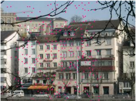
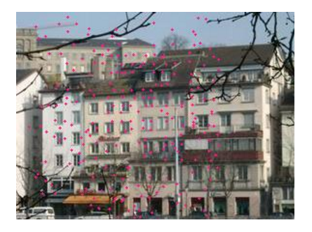
Figure 1. An example of image from the ZuBuD dataset. The left image is the original query where 424 features are detected, while the right image shows the cropped verison with 367 featured retained.

One of the weakness of classical VLAD in landmark recognition is due to the noisy features corresponding to distractors such as trees, traffic signs, cars, people, etc. The proposed variant of VLAD, called locVLAD (location-aware VLAD), tackles this problem by reducing the influence of features found at the borders of the image. One important point to make is that we do not simply remove features at the image borders, but fuse them at the VLAD descriptor level. The VLAD procedure described above is performed twice (only on test phase), one considering the whole image, and the other considering the images cropped of a certain percentage. It is quite straightforward (but important) to notice that, by repeating the whole pipeline, the feature set $x$ and, therefore, the VLAD vectors will be different. For instance, Fig. 1 shows how the detected features change. Once the two VLAD vectors (denoted with $\mathbf{\dot{v}}$ and $\mathbf{\dot{v}_{cropped}}$) are computed, the locVLAD vector is simply obtained by averaging them:

(1) $$\mathbf{\dot{v}_{locVLAD}}=\frac{\mathbf{\dot{v}}+\mathbf{\dot{v}_{cropped}}}{2}$$

There are two main parameters to account for: the weights for the two vectors $\mathbf{\dot{v}}$ and $\mathbf{\dot{v}_{cropped}}$, and the percentage of borders to be cropped. Regarding the former, we performed different tests and realized that the best results are obtained by an equal weight for the two vectors, as shown in equation 1. The second parameter depends on the resolution of the images in the dataset and will be discussed in the experiments. The rationale behind our proposal is that the most important features (useful to recognize the landmark) are located near the center of the image, whereas the distractors are often at the border of the image (see, for instance, Fig. 1).

The above rationale might not be always true, i.e. some features at the image borders might be useful. For this reasone we average both the cropped and not-cropped VLAD descriptors. However, locVLAD procedure is not applied to the database images. Although this could be reasonable, experiments demonstrate that applying it also on the database images decreases the recognition accuracy. This behaviour can be explained by the fact that the database contains different views of the same landmark, also zoomed views. In these latter cases the significant features are located at the borders too and should not be removed. Therefore, the best results are achieved by applying locVLAD encoding on the query images only.

4. Experimental results

In order to evaluate the accuracy of the proposed embedding technique with respect to the state of the art, we run experiments on public datasets and employing standard evaluation metrics.

4.1. Datasets and metrics

The performance is measured on two public image datasets: ZuBuD and Holidays.

ZuBuD (Zurich, 2003) is composed by 1005 images of the size of 640x480 (or 480x640 if they are rotated), subdivided in 201 classes, about the building of Zurich. The query images are 115 and they are of the size of 320x240. Not all the classes are represented in the query set, but only 85.

Since not all the classes are represented in the query set, in order to have a more balanced dataset, we created a new version of ZuBuD, called ZuBuD+ (available at http://implab.ce.unipr.it/?page_id=194). While keeping the database images unchanged, we extended the query images by randomly selecting images of the missing classes and transforming them by resizing and rotating them with ±90°. The total number of query images is raised to 1005 and all the classes are equally represented (5 queries per class). Fig. 2 shows some examples of the newly-added query images. According to (Zhang et al., 2015), to increase the recognition accuracy, we resized the database images to 320x240 (or 240x320 if they are rotated) during the creation of VLAD vectors for the database images.

Holidays (Jégou et al., 2008) is composed of 1491 high-resolution images representing the holiday photos of different locations and objects, subdivided in 500 classes. The database images are 991 and the query images are 500, one for every class.

Vocabulary creation. The vocabulary on both ZuBuD and ZuBuD+ (because they have the same training images) is created by using all the features detected (about 208k features) since the images are few and of limited resolution. Conversely, Holidays is a larger dataset with higher resolution images and using all the features would result in a very large vocabulary. Therefore, we downsampled the number of features by randomly selecting 1/5 of the detected features (1.84 M out of the total features). On the downsampled set of features, K-Means++ (an approximated version of K-Means clustering for NP-hard problems) (Arthur and Vassilvitskii, 2007) is applied. The use of less features has a twofold motivation: first, it reduces computational time; second, it allows to reduce the chance of overfitting problem by supposedly avoiding to include features of the query images in the vocabulary. Finally, by randomly selecting the features to be retained (instead of selecting the first N features), we can avoid to overtrain on a particular patch.

Figure 2. Example of data added in the query set of ZuBuD.

Size of cropped images. As mentioned in the previous chapter the locVLAD approach is based on a mean of two VLAD descriptors: the VLAD on the original image and the one on the cropped image. The size of the cropped image have different values for every dataset used in the experiments. Before getting the best results, we tried different values. The best values are shown in Table 1.

Table 1. Size of cropped images used for the application of locVLAD

Dataset	Size of cropped image
ZuBuD and ZuBuD+	90% of the original images’ size
Holidays	70% of the original images’ size

Metrics. Standard evaluation metrics include the mean average precision (mAP) or some ranking-based metrics, such as Top1 or 5xRecall@Top5 (average of how many times the correct image is in the top 5 results in the ranking). For the Holidays dataset we used the mAP provided by the corresponding evaluation tool, whereas for ZuBuD we prefered the ranking-based metrics which have been used in the compared works.

Distance. In order to compare a query image with the database, a $L_{2}$ distance is employed. An alternative distance is the cosine similarity, but results are similar and the computation is slower than the $L_{2}$ distance.

Implementation. In term of actual implementation, the detector and descriptor used is SiftGPU (Wu, 2007), that runs on GPU on a NVIDIA GeForce GTX 1070 mounted on a computer with a 8-core 3.40GHz CPU.

4.2. Results on ZuBuD+

Table 2. Comparison with the state of the art on ZuBuD and ZuBuD+ dataset

Method	Descriptor size	Top1	5xRecall@Top5
Tree histogram (ZuBuD) (Chen et al., 2009)	10M	98.00%	-
Decision tree (ZuBuD) (Fritz et al., 2006)	n/a	91.00%	-
Sparse coding (ZuBuD) (Zhang et al., 2015)	8k*64+1k*36	-	4.538
VLAD (ZuBuD) (Jégou et al., 2010)	4281*128	99.00%	4.416
VLAD (ZuBuD+) (Jégou et al., 2010)	4281*128	99.00%	4.526
locVLAD (ZuBuD)	4281*128	100.00%	4.469
locVLAD (ZuBuD+)	4281*128	100.00%	4.543

We run the first set of experiments on the balanced dataset ZuBuD+. We compared the proposed locVLAD with standard VLAD as baseline. Moreover, we also compared our approach with published results on ZuBuD from three state-of-the-art papers. The tree histogram approach proposed in (Chen et al., 2009) uses a vocabulary of $10M$ visual words. Instead, the approach presented in (Fritz et al., 2006) is based on decision trees and the i-SIFT detector described above. Finally, the third method compared (Zhang et al., 2015) is based on sparse coding. In terms of vocabulary size (which an important parameter to compare having a direct effect on the recognition accuracy and the computational complexity of the approach), the first method (Chen et al., 2009) uses very large vocabulary so they can not be fairly compared with our (which is much more compact) and the second (Fritz et al., 2006) does not use a vocabulary. However, as shown in Table 2, the locVLAD approach can obtain superior results on top1 even using a smaller vocabulary ($4281$ wrt $10M$ for (Chen et al., 2009)). Conversely, in the case of sparse coding in (Zhang et al., 2015), a vocabulary composed of $8k$ $64-D$ SURF descriptors plus $1k$ color descriptors is used. In order to perform a fair comparison, also locVLAD is tested with a vocabulary of the same size, i.e $64*8k+36*1k=548k$. Since we are using $128-D$ SIFT descriptors, this means about $4281$ visual words.

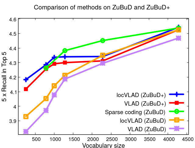
Figure 3. We compare VLAD and locVLAD with the method based on sparse coding, using different vocabulary size on ZuBuD and ZuBuD+.

Table 2 shows the results of locVLAD compared with baseline VLAD and sparse coding (Zhang et al., 2015) with the same vocabulary size and on 5xRecall@Top5, while the comparison with (Chen et al., 2009; Fritz et al., 2006) is done at completely different sizes and on Top1. For locVLAD both results on ZuBuD and ZuBuD+ are shown. It is evident that our method outperforms (Chen et al., 2009; Fritz et al., 2006) and baseline VLAD, and that for the first two it is also using a much small vocabulary. However, our results compared with sparse coding are slightly worse when applied on ZuBuD. This can be explained by the unbalance in the query set described above. When applied on ZuBuD+, locVLAD outperforms the sparse coding results. This is also confirmed in Fig. 3 where we reported the comparison with the baseline VLAD and sparse coding at different vocabulary sizes.

4.3. Results on Holidays

In similar way, we run experiments on the Holidays dataset. As before, we compared with both the baseline VLAD and state-of-the-art methods. In this case, we compared again with (Zhang et al., 2015) which uses sparse coding and max-pooling and with another paper (Cao et al., 2012) using again sparse coding but with geometric pooling, i.e. local descriptors sharing good geometric consistency are pooled together to ensure a more precise spatial layouts. As we did for ZuBuD, we set the vocabulary size to be comparable to that of the compared methods, i.e $4281$ for (Zhang et al., 2015) and $20k$ for (Cao et al., 2012).

Table 3. Comparison with the state of the art on Holidays dataset with different feature vectors size

Method	Descriptor size	mAP
Sparse coding (Zhang et al., 2015)	8k*64+1k*36	76.51%
VLAD (Jégou et al., 2010)	4281*128	74.43%
locVLAD	4281*128	77.20%
Sparse coding (Cao et al., 2012)	20k*128	79.00%
VLAD (Jégou et al., 2010)	20k*128	78.78%
locVLAD	20k*128	80.89%

In fact, in this last case, the number $K$ of visual words is set to $20k$. Table 3 shows the results and clearly demonstrates that the proposed locVLAD achieves better mAP than the other methods.

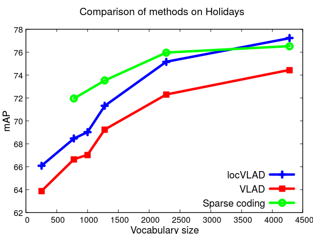
Figure 4. We compare VLAD and locVLAD with the method based on sparse coding, using different vocabulary size on Holidays.

As we showed in Fig. 3, Fig. 4 shows the different values of mAP achieved by baseline VLAD, sparse coding (Zhang et al., 2015) and locVLAD at different vocabulary sizes. Finally, Fig. 5 shows the computational time needed for clustering at different vocabulary sizes when all the features compared with the $1/5$ downsampled features are used. As expected, the computational time increases very quickly when using all the features.

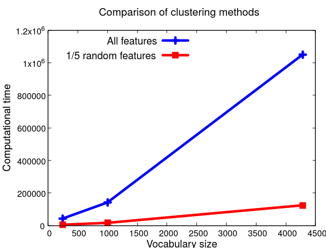
Figure 5. Computational time in the clustering phase on Holidays dataset. The vocabulary size choosen are: $250$, $1000$ and $4281$.

5. Conclusions

This paper proposes a novel embedding technique for efficient and effective landmark recognition. The proposed locVLAD technique includes, at a certain degree, information on the location of the features, by mitigating the negative efects of distractors found at the image borders. Experiments are performed on two public datasets, namely ZuBuD and Holidays, and demonstrates superior recognition accuracy wrt the state of the art. It is worth to note that on ZuBuD the method based on sparse coding in (Zhang et al., 2015) slightly outperforms the proposed one. This is due to an unbalanced query set and, probably, on the use of color information (which is not used in our approach). However, the results on both a more balanced dataset (ZuBuD+) and on the other dataset (Holidays) show that our method works better than (Zhang et al., 2015), substantially confirming our above-reported explanation.

Acknowledgments. This work is partially funded by Regione Emilia Romagna under the “Piano triennale alte competenze per la ricerca, il trasferimento tecnologico e l’imprenditorialità”.

References

- (1)
- Arandjelović and Zisserman (2012) Relja Arandjelović and Andrew Zisserman. 2012. Three things everyone should know to improve object retrieval. In Computer Vision and Pattern Recognition (CVPR), 2012 IEEE Conference on. IEEE, 2911–2918.
- Arandjelovic and Zisserman (2013) Relja Arandjelovic and Andrew Zisserman. 2013. All about VLAD. In Proceedings of the IEEE Conference on Computer Vision and Pattern Recognition. 1578–1585.
- Arthur and Vassilvitskii (2007) David Arthur and Sergei Vassilvitskii. 2007. k-means++: The advantages of careful seeding. In Proceedings of the eighteenth annual ACM-SIAM symposium on Discrete algorithms. Society for Industrial and Applied Mathematics, 1027–1035.
- Cao et al. (2012) Liujuan Cao, Rongrong Ji, Yue Gao, Yi Yang, and Qi Tian. 2012. Weakly supervised sparse coding with geometric consistency pooling. In Computer Vision and Pattern Recognition (CVPR), 2012 IEEE Conference on. IEEE, 3578–3585.
- Chen et al. (2013) David Chen, Sam Tsai, Vijay Chandrasekhar, Gabriel Takacs, Ramakrishna Vedantham, Radek Grzeszczuk, and Bernd Girod. 2013. Residual enhanced visual vector as a compact signature for mobile visual search. Signal Processing 93, 8 (2013), 2316–2327.
- Chen et al. (2011) David M Chen, Georges Baatz, Kevin Koser, Sam S Tsai, Ramakrishna Vedantham, Timo Pylvanainen, Kimmo Roimela, Xin Chen, Jeff Bach, Marc Pollefeys, and others. 2011. City-scale landmark identification on mobile devices. In Computer Vision and Pattern Recognition (CVPR), 2011 IEEE Conference on. IEEE, 737–744.
- Chen et al. (2009) David M Chen, Sam S Tsai, Vijay Chandrasekhar, Gabriel Takacs, Jatinder Singh, and Bernd Girod. 2009. Tree histogram coding for mobile image matching. In Data Compression Conference, 2009. DCC’09. IEEE, 143–152.
- Delhumeau et al. (2013) Jonathan Delhumeau, Philippe-Henri Gosselin, Hervé Jégou, and Patrick Pérez. 2013. Revisiting the VLAD image representation. In Proceedings of the 21st ACM international conference on Multimedia. ACM, 653–656.
- Fritz et al. (2006) Gerald Fritz, Christin Seifert, and Lucas Paletta. 2006. A mobile vision system for urban detection with informative local descriptors. In Computer Vision Systems, 2006 ICVS’06. IEEE International Conference on. IEEE, 30–30.
- Gong et al. (2014) Yunchao Gong, Liwei Wang, Ruiqi Guo, and Svetlana Lazebnik. 2014. Multi-scale orderless pooling of deep convolutional activation features. In European conference on computer vision. Springer, 392–407.
- Jégou et al. (2008) Hervé Jégou, Matthijs Douze, and Cordelia Schmid. 2008. Hamming embedding and weak geometry consistency for large scale image search-extended version. (2008).
- Jégou et al. (2010) Hervé Jégou, Matthijs Douze, Cordelia Schmid, and Patrick Pérez. 2010. Aggregating local descriptors into a compact image representation. In Computer Vision and Pattern Recognition (CVPR), 2010 IEEE Conference on. IEEE, 3304–3311.
- Jegou et al. (2012) Herve Jegou, Florent Perronnin, Matthijs Douze, Jorge Sánchez, Patrick Perez, and Cordelia Schmid. 2012. Aggregating local image descriptors into compact codes. IEEE transactions on pattern analysis and machine intelligence 34, 9 (2012), 1704–1716.
- Nister and Stewenius (2006) David Nister and Henrik Stewenius. 2006. Scalable recognition with a vocabulary tree. In Computer vision and pattern recognition, 2006 IEEE computer society conference on, Vol. 2. Ieee, 2161–2168.
- Perronnin and Dance (2007) Florent Perronnin and Christopher Dance. 2007. Fisher kernels on visual vocabularies for image categorization. In Computer Vision and Pattern Recognition, 2007. CVPR’07. IEEE Conference on. IEEE, 1–8.
- Perronnin et al. (2010) Florent Perronnin, Jorge Sánchez, and Thomas Mensink. 2010. Improving the fisher kernel for large-scale image classification. In European conference on computer vision. Springer, 143–156.
- Schroth et al. (2011) Georg Schroth, Anas Al-Nuaimi, Robert Huitl, Florian Schweiger, and Eckehard Steinbach. 2011. Rapid image retrieval for mobile location recognition. In Acoustics, Speech and Signal Processing (ICASSP), 2011 IEEE International Conference on. IEEE, 2320–2323.
- Sharif Razavian et al. (2014) Ali Sharif Razavian, Hossein Azizpour, Josephine Sullivan, and Stefan Carlsson. 2014. CNN features off-the-shelf: an astounding baseline for recognition. In Proceedings of the IEEE Conference on Computer Vision and Pattern Recognition Workshops. 806–813.
- Sivic et al. (2003) Josef Sivic, Andrew Zisserman, and others. 2003. Video google: A text retrieval approach to object matching in videos.. In iccv, Vol. 2. 1470–1477.
- Spyromitros-Xioufis et al. (2014) Eleftherios Spyromitros-Xioufis, Symeon Papadopoulos, Ioannis Yiannis Kompatsiaris, Grigorios Tsoumakas, and Ioannis Vlahavas. 2014. A comprehensive study over vlad and product quantization in large-scale image retrieval. IEEE Transactions on Multimedia 16, 6 (2014), 1713–1728.
- Wu (2007) Changchang Wu. 2007. SiftGPU: A GPU Implementation of Scale Invariant Feature Transform (SIFT). http://cs.unc.edu/~ccwu/siftgpu. (2007).
- Zhang et al. (2015) Yunchao Zhang, Jing Chen, Xiujie Huang, and Yongtian Wang. 2015. A Probabilistic Analysis of Sparse Coded Feature Pooling and Its Application for Image Retrieval. PloS one 10, 7 (2015), e0131721.
- Zhao et al. (2013) Wan-Lei Zhao, Hervé Jégou, and Guillaume Gravier. 2013. Oriented pooling for dense and non-dense rotation-invariant features. In BMVC-24th British machine vision conference.
- Zurich (2003) ETH Zurich. 2003. ZuBuD: Zurich Building Dataset. http://www.vision.ee.ethz.ch/showroom/zubud/. (2003).