Keldysh Derivation of Oguri’s Linear Conductance Formula for Interacting Fermions

Jan Heyder    Florian Bauer    Dennis Schimmel    Jan von Delft Arnold Sommerfeld Center for Theoretical Physics and Center for NanoScience, Ludwig-Maximilians-Universität München, Theresienstrasse 37, D-80333 München, Germany
(April 12, 2017)
Abstract

We present a Keldysh-based derivation of a formula, previously obtained by Oguri using the Matsubara formalisum, for the linear conductance through a central, interacting region coupled to non-interacting fermionic leads. Our starting point is the well-known Meir-Wingreen formula for the current, whose derivative w.r.t. to the source-drain voltage yields the conductance. We perform this derivative analytically, by exploiting an exact flow equation from the functional renormalization group, which expresses the flow w.r.t. voltage of the self-energy in terms of the two-particle vertex. This yields a Keldysh-based formulation of Oguri’s formula for the linear conductance, which facilitates applying it in the context of approximation schemes formulated in the Keldysh formalism. (Generalizing our approach to the non-linear conductance is straightforward, but not pursued here.) – We illustrate our linear conductance formula within the context of a model that has previously been shown to capture the essential physics of a quantum point contact in the regime of the 0.7 anomaly. The model involves a tight-binding chain with a one-dimensional potential barrier and onsite interactions, which we treat using second order perturbation theory. We show that numerical costs can be reduced significantly by using a non-uniform lattice spacing, chosen such that the occurence of artificial bound states close to the upper band edge is avoided.

I Introduction

Two cornerstones of the theoretical description of transport through a mesoscopic system are the Landauer-Büttiker Landauer (1957) and Meir-Wingreen Meir and Wingreen (1992) formulas for the conductance. The Landauer-Büttiker formula describes the conductance between two reservoirs connected by a central region in the absence of interactions. The Meir-Wingreen formula applies to the more general case that the central region contains electron-electron interactions: it expresses the current, in beautifully compact fashion, in terms of the Fermi functions of the reservoirs, and the retarded, advanced and Keldysh components of the Green’s function for the central region.

To actually apply the Meir-Wingreen formula, these Green’s functions have to be calculated explicitly, which in general is a challenging task. Depending on the intended application, a wide range of different theoretical tools have been employed for this purpose. Much attention has been lavished on the case of non-equilibrium transport through a quantum dot described by a Kondo or Anderson model, where the central interacting region consists of just a single localized spin or a single electronic level, see Refs. Eckel et al. (2010); Andergassen et al. (2010) for reviews. Here we are interested in the less well-studied case of systems for which the physics of the interacting region cannot be described by just a single site, but rather requires an extended model, consisting of many sites.

We have recently used a model of this type in a paper that offers an explanation for the microscopic origin of the 0.7-anomaly in the conductance through a quantum point contact (QPC) Bauer et al. (2013). The model involves a tight-binding chain with a one-dimensional potential barrier and onsite interactions. In Ref. Bauer et al. (2013) we used two approaches to treat interactions: second-order perturbation theory (SOPT) and the functional renormalization group (fRG). Our calculations of the linear conductance were based on an exact formula derived by Oguri Oguri (2001a, 2003). He started from the Kubo formula in the Matsubara formalism and performed the required analytical continuation of the two-particle vertex function occurring therein using Eliashberg theory Eliashberg (1962).

Since Oguri’s formula for the linear conductance is exact, it can also be used when employing methods different from SOPT, for example fRG, to calculate the self-energy and two-particle vertex. If this is done in the Matsubara formalism, and if one attempts to capture the frequency dependence of the self-energy (as for the fRG calculations of Ref. Bauer et al. (2013)), one is limited, in practice, to the case of zero temperature, because finite-temperature calculations would require an analytic continuation of numerical data from the imaginary to the real frequency axis, which is a mathematically ill-defined problem. This problem can be avoided by calculating the self-energy and vertex directly on the real axis using the Keldysh formalism Keldysh (1964); Kamenev and Levchenko (2009). However, to then calculate the linear conductance, the ingredients occuring in Oguri’s formula would have to be transcribed into Keldysh language, and such a transcription is currently not available in the literature in easily accessible form.

The main goal of the present paper is to derive a Keldysh version of Oguri’s formula for the linear conductance by working entirely within the Keldysh formalism. Our starting point is the Meir-Wingreen formula for the current, $J(V)$, with the conductance defined by $\text{g}=\partial_{V}J$. Rather than performing this derivative numerically, we here perform it analytically, based on the following central observation: The voltage derivative of the Green’s functions that occur in the Meir-Wingreen formula, $\partial_{V}\mathcal{G}$, all involve the voltage derivative of the self-energy, $\partial_{V}\Sigma$. The latter can be expressed in terms of the two-particle vertex by using an exact flow equation from the fRG. (Analogous strategies have been used in the past for the dependence of the self-energy on temperature Honerkamp and Salmhofer (2001) or chemical potential Sauli and Kopietz (2006); Jakobs et al. (2007a).) We show that it is possible to use this observation to derive Oguri’s formula for the linear conductance, expressed in Keldysh notation, provided that the Hamiltonian is symmetric and conserves particle number. Our argument evokes a Ward identity Ward (1950), following from $U(1)$-symmetry, which provides a relation between components of the self-energy and components of the vertex.

As an application of our Keldysh version of Oguri’s conductance formula, we use Keldysh-SOPT to calculate the conductance through a QPC using the model of Ref. Bauer et al. (2013). Some results of this type were already presented in Ref. Bauer et al. (2013), but without offering a detailed account of the underlying formalism. Providing these detail is one of the goals of the present paper. We also discuss some details of the numerical implementation of these calculations. In particular, we show that it is possible to greatly reduce the numerical costs by using a non-monotonic lattice spacing when formulating the discretized model. We present results for the conductance as function of barrier height for different choices of interaction strength $U$, magnetic field $B$ and temperature $T$ and discuss both the successes and limitations of the SOPT scheme.

The paper is organized as follows: After introducing the general interacting model Hamiltonian in Sec. II, we present the Keldysh derivation of Oguri’s conductance formula in Sec. III. We set the stage for explicit conductance calculations by expressing the self-energy and the two-particle vertex within Keldysh SOPT in Sec. IV. We introduce our the 1D-model of a QPC and discuss results for the conductance in Sec. V. A detailed collection of definitions and properties of both Green’s and vertex functions in the Keldysh formalism can be found in Appendix A and in Ref. Jakobs et al. (2010) (in fact our paper closely follows the notation used therein). A diagrammatic derivation of the fRG flow-equation for the self-energy is given in Appendix B and the Ward identity resulting from particle conservation is presented in Appendix C. In Appendix D we perform an explicit calculation to verify the fluctuation-dissipation theorem for the vertex-functions within SOPT. Finally, we apply the method of finite differences in Appendix E, to discretize the continuous Hamiltonian using a non-constant discretization scheme.

II Microscopic model

Within this work we consider a system composed of a finite central interacting region coupled to two non-interacting semi-infinite fermionic leads, a left lead, with chemical potential $\mu^{l}$, temperature $T^{l}$ and Fermi-distribution function $f^{l}$, and a right lead, with chemical potential $\mu^{r}$, temperature $T^{r}$ and Fermi-distribution function $f^{r}$. The two leads are not directly connected to each other, but only via the central region. A similar setup was considered in Ref. Meir and Wingreen (1992) and Ref. Oguri (2001a).

The general form of the model Hamiltonian reads

$${H}={H}_{{\color[rgb]{0,.5,0}\textbf{0}}}+{H}_{\rm{int}}=\sum_{\color[rgb]{0,0,1}ij}h_{{\color[rgb]{0,0,1}ij}}d_{{\color[rgb]{0,0,1}i}}^{\dagger}d_{{\color[rgb]{0,0,1}j}}+\sum_{{\color[rgb]{0,0,1}ij}}U_{{\color[rgb]{0,0,1}ij}}n_{{\color[rgb]{0,0,1}i}}n_{{\color[rgb]{0,0,1}j}}\;,$$ (1)

where $h_{{\color[rgb]{0,0,1}ij}}$ is a hermitian matrix, and $U_{{\color[rgb]{0,0,1}ij}}$ is a real, symmetric matrix, non-zero only for states $\color[rgb]{0,0,1}i$,$\color[rgb]{0,0,1}j$ within the central region. $d_{{\color[rgb]{0,0,1}i}}^{\dagger}$/$d_{{\color[rgb]{0,0,1}i}}$ creates/destroys an electron in state $\color[rgb]{0,0,1}i$ and $n_{{\color[rgb]{0,0,1}i}}=d_{{\color[rgb]{0,0,1}i}}^{\dagger}d_{{\color[rgb]{0,0,1}i}}$ counts the number of electrons in state $\color[rgb]{0,0,1}i$. While in general the index $\color[rgb]{0,0,1}i$ can represent any set of quantum numbers we will regard it as a composite index, referring, e.g. to the site and spin of an electron for a spinful lattice model. Note, that the Hamiltonian conserves particle number, which is crucial in order to formulate a continuity equation for the charge current in the system.

We use a block representation of the matrix $h$ of the single-particle Hamiltonian

$\displaystyle{h}\!=\!\left(\begin{array}[]{ccc}{h}_{l}&{h}_{lc}&0\\ \leavevmode\nobreak\ \!\!{h}_{cl}&{h}_{{\color[rgb]{0,.5,0}\textbf{0}},c}&{h}_{cr}\\ 0&{h}_{rc}&{h}_{r}\\ \end{array}\right),$ (5)

where the indices $l$, $r$, and $c$ stand for the left lead, right lead, and central region, respectively. For example, the spatial indices of the matrix ${h}_{{\color[rgb]{0,.5,0}\textbf{0}},c}$ both take values only within the central region, while the first spatial index of ${h}_{cl}$ takes a value within the central region and the second spatial index takes a value within the left lead. The subscript 00 emphasizes the absence of interactions in the definition of ${h}_{{\color[rgb]{0,.5,0}\textbf{0}},c}$ (the leads and the coupling between the leads and the central region are assumed non-interacting throughout the whole paper).

III Transport formulas

We henceforth work in the Keldysh formalism. Our notation for Keldysh indices, which mostly follows that of Ref. Jakobs et al. (2010), is set forth in detail in Appendix A, to allow the main text to focus only on the essential steps of the argument.

III.1 Current formula

We begin by retracing the derivation of the Meir-Wingreen formula. In steady state the number of particles in the central region is constant. Hence, the particle current from the left lead into the central region is equal to the particle current from the central region into the right lead, $J:=J_{l\to c}=J_{c\to r}$. [We remark that this continuity equation can also be obtained by imposing the invariance of the partition sum under a gauged $U(1)$ transformation, following from particle conservation of the Hamiltonian, see Appendix C]. This allows us to focus on the current through the interface between left lead and central region. Expressing the current in terms of the time-derivative of the total particle number operator of the left lead, $n_{l}=\sum_{{\color[rgb]{0,0,1}i}\in L}n_{{\color[rgb]{0,0,1}i}}$, we obtain the Heisenberg equation of motion $J=-e\langle\dot{n}_{l}\rangle=-ie/\hbar\langle[{H},n_{l}]\rangle$, where $e$ is the electronic charge and $\hbar$ is Planck’s constant. For the Hamiltonian of Eq. (1), the current thus reads

$\displaystyle J$ $\displaystyle=-\frac{ie}{\hbar}\!\sum_{\underset{{\color[rgb]{0,0,1}j}\in C}{{\color[rgb]{0,0,1}i}\in L}}\left[h_{{\color[rgb]{0,0,1}ij}}\langle d_{\mathchoice{\raisebox{-2.5pt}{$\displaystyle{\color[rgb]{0,0,1}j}$}}{\raisebox{-2.5pt}{$\textstyle{\color[rgb]{0,0,1}j}$}}{\raisebox{-2.5pt}{$\scriptstyle{\color[rgb]{0,0,1}j}$}}{\raisebox{-2.5pt}{$\scriptscriptstyle{\color[rgb]{0,0,1}j}$}}}^{{\color[rgb]{1,0,0}-}}(t)[d_{{\color[rgb]{0,0,1}i}}^{\color[rgb]{1,0,0}+}]^{\dagger}(t)\rangle-h_{{\color[rgb]{0,0,1}ji}}\langle d_{\mathchoice{\raisebox{-2.5pt}{$\displaystyle{\color[rgb]{0,0,1}i}$}}{\raisebox{-2.5pt}{$\textstyle{\color[rgb]{0,0,1}i}$}}{\raisebox{-2.5pt}{$\scriptstyle{\color[rgb]{0,0,1}i}$}}{\raisebox{-2.5pt}{$\scriptscriptstyle{\color[rgb]{0,0,1}i}$}}}^{{\color[rgb]{1,0,0}-}}(t)[d_{{\color[rgb]{0,0,1}j}}^{\color[rgb]{1,0,0}+}]^{\dagger}(t)\rangle\right]$
$\displaystyle=\!\frac{e}{\hbar}\left[{\rm{Tr}}\{({h}_{lc}-{h}_{cl})G^{{\color[rgb]{1,0,0}-}|{\color[rgb]{1,0,0}+}}\}\right],$ (6)

with the interacting equal-time lesser Green’s function $G_{{\color[rgb]{0,0,1}i}|{\color[rgb]{0,0,1}j}}^{{\color[rgb]{1,0,0}-}|{\color[rgb]{1,0,0}+}}\!=\!G_{{\color[rgb]{0,0,1}i}|{\color[rgb]{0,0,1}j}}^{{\color[rgb]{1,0,0}-}|{\color[rgb]{1,0,0}+}}(t|t)\!=\!-i\langle d_{\mathchoice{\raisebox{-2.5pt}{$\displaystyle{\color[rgb]{0,0,1}i}$}}{\raisebox{-2.5pt}{$\textstyle{\color[rgb]{0,0,1}i}$}}{\raisebox{-2.5pt}{$\scriptstyle{\color[rgb]{0,0,1}i}$}}{\raisebox{-2.5pt}{$\scriptscriptstyle{\color[rgb]{0,0,1}i}$}}}^{{\color[rgb]{1,0,0}-}}(t)[d_{{\color[rgb]{0,0,1}j}}^{\color[rgb]{1,0,0}+}]^{\dagger}(t)\rangle$ (here we used time-translational invariance of the steady-state). Fourier transformation of Eq. (6) yields

$\displaystyle J=\frac{e}{h}\!\int\!\!d\varepsilon\!\leavevmode\nobreak\ {\rm{Tr}}\big{\{}({h}_{lc}-{h}_{cl})\mathcal{G}^{{\color[rgb]{1,0,0}-}|{\color[rgb]{1,0,0}+}}(\varepsilon)\big{\}},$ (7)

with $h\!=\!2\pi\hbar$. We introduced the symbol $\mathcal{G}$ for a Green’s function that depends on a single frequency only (as opposed to the Fourier transform of the time-dependent Green’s function $G$, which, in general, depends on two frequencies, see Appendix A, Eq. (A.7), for details).

Following the strategy of Ref. Meir and Wingreen (1992), we use Dyson’s equation, Eq. (A.51), to express the current in terms of the central region Green’s function $\mathcal{G}_{c}$ and rotate from the contour basis into the Keldysh basis (the explicit Keldysh rotation is given by Eq. (A.14) and Eq. (A.27c)). This yields

$$J\!=\!\frac{ie}{2h}\!\int\!\!d\varepsilon\leavevmode\nobreak\ {\rm Tr}\{\Gamma^{l}[\mathcal{G}_{c}^{{\color[rgb]{1,0,0}2}|{\color[rgb]{1,0,0}2}}-(1-2f^{l})(\mathcal{G}_{c}^{{\color[rgb]{1,0,0}2}|{\color[rgb]{1,0,0}1}}-\mathcal{G}_{c}^{{\color[rgb]{1,0,0}1}|{\color[rgb]{1,0,0}2}})]\},$$ (8)

with retarded, $\mathcal{G}_{c}^{{\color[rgb]{1,0,0}2}|{\color[rgb]{1,0,0}1}}(\varepsilon)$, advanced, $\mathcal{G}_{c}^{{\color[rgb]{1,0,0}1}|{\color[rgb]{1,0,0}2}}(\varepsilon)$, and Keldysh central region Green’s function, $\mathcal{G}_{c}^{{\color[rgb]{1,0,0}2}|{\color[rgb]{1,0,0}2}}(\varepsilon)$, and the hybridization function $\Gamma^{l}(\varepsilon)\!=\!i\leavevmode\nobreak\ h_{cl}(g_{l}^{{\color[rgb]{1,0,0}2}|{\color[rgb]{1,0,0}1}}(\varepsilon)\!-\!g_{l}^{{\color[rgb]{1,0,0}1}|{\color[rgb]{1,0,0}2}}(\varepsilon))h_{lc}$, where $g_{l}(\varepsilon)$ is the Green’s function of the isolated left lead. Here and below we omit the frequency argument for all quantities that depend on the integration variable only. Eq. (8) is the celebrated Meir-Wingreen formula for the current (c.f. Eq. (6) in Ref. Meir and Wingreen (1992) for a symmetrized version thereof).

We now present a version of the Meir-Wingreen formula in terms of the interacting one-particle irreducible self-energy $\Sigma$ (with retarded, $\Sigma^{{\color[rgb]{1,0,0}1}|{\color[rgb]{1,0,0}2}}$, advanced, $\Sigma^{{\color[rgb]{1,0,0}2}|{\color[rgb]{1,0,0}1}}$ and Keldysh component $\Sigma^{{\color[rgb]{1,0,0}1}|{\color[rgb]{1,0,0}1}}$ [Eq. (A.3), Eq. (A.7), Eq. (A.26)]). It can be derived by means of Dyson’s equation, Eq. (A.50), which enables a reformulation of the Green’s functions in Eq. (8) in terms of the hybridization functions $\Gamma$, the lead distribution functions $f$ and the self-energy $\Sigma$:

$\displaystyle\mathcal{G}_{c}^{{\color[rgb]{1,0,0}2}|{\color[rgb]{1,0,0}1}}\!-\!\mathcal{G}_{c}^{{\color[rgb]{1,0,0}1}|{\color[rgb]{1,0,0}2}}=\mathcal{G}_{c}^{{\color[rgb]{1,0,0}2}|{\color[rgb]{1,0,0}1}}\big{(}\big{[}\mathcal{G}_{c}^{{\color[rgb]{1,0,0}1}|{\color[rgb]{1,0,0}2}}\big{]}^{-1}\!-\big{[}\mathcal{G}_{c}^{{\color[rgb]{1,0,0}2}|{\color[rgb]{1,0,0}1}}\big{]}^{-1}\big{)}\mathcal{G}_{c}^{{\color[rgb]{1,0,0}1}|{\color[rgb]{1,0,0}2}}$
$\displaystyle\quad\quad\quad\quad\leavevmode\nobreak\ =\mathcal{G}_{c}^{{\color[rgb]{1,0,0}2}|{\color[rgb]{1,0,0}1}}\big{(}-i(\Gamma^{l}+\Gamma^{r})+\!\Sigma^{{\color[rgb]{1,0,0}1}|{\color[rgb]{1,0,0}2}}-\Sigma^{{\color[rgb]{1,0,0}2}|{\color[rgb]{1,0,0}1}}\big{)}\mathcal{G}_{c}^{{\color[rgb]{1,0,0}1}|{\color[rgb]{1,0,0}2}},$
$\displaystyle\mathcal{G}_{c}^{{\color[rgb]{1,0,0}2}|{\color[rgb]{1,0,0}2}}\!=\!\mathcal{G}_{c}^{{\color[rgb]{1,0,0}2}|{\color[rgb]{1,0,0}1}}\!\big{(}-i\sum_{k=l,r}(1-2f^{k})\Gamma^{k}+\!\Sigma^{{\color[rgb]{1,0,0}1}|{\color[rgb]{1,0,0}1}}\big{)}\mathcal{G}_{c}^{{\color[rgb]{1,0,0}1}|{\color[rgb]{1,0,0}2}}.$ (9)

Hence, the current formula can be written as the sum of two terms,

$\displaystyle J=$ $\displaystyle\frac{e}{h}\int\!d\varepsilon\Bigl{[}(f^{l}-f^{r}){\rm Tr}\{\Gamma^{l}\mathcal{G}_{c}^{{\color[rgb]{1,0,0}2}|{\color[rgb]{1,0,0}1}}\Gamma^{r}\mathcal{G}_{c}^{{\color[rgb]{1,0,0}1}|{\color[rgb]{1,0,0}2}}\}+$ (10)
$\displaystyle\;\;\Bigl{.}+\frac{i}{2}{\rm Tr}\{\Gamma^{l}\mathcal{G}_{c}^{{\color[rgb]{1,0,0}2}|{\color[rgb]{1,0,0}1}}\!\left(\!\Sigma^{{\color[rgb]{1,0,0}1}|{\color[rgb]{1,0,0}1}}-(1\!-\!2f^{l})(\Sigma^{{\color[rgb]{1,0,0}1}|{\color[rgb]{1,0,0}2}}-\Sigma^{{\color[rgb]{1,0,0}2}|{\color[rgb]{1,0,0}1}})\right)\!\mathcal{G}_{c}^{{\color[rgb]{1,0,0}1}|{\color[rgb]{1,0,0}2}}\}\Bigr{]}.$

In equilibrium, i.e.​ $f\!:=\!f^{l}\!=\!f^{r}$, the current must fulfill $J\!=\!0$. With the first term of Eq. (10) vanishing trivially, this imposes the fluctuation-dissipation theorem (FDT) for the self-energy at zero bias voltage, $\Sigma^{{\color[rgb]{1,0,0}1}|{\color[rgb]{1,0,0}1}}\!=\!(1\!-\!2f)(\Sigma^{{\color[rgb]{1,0,0}1}|{\color[rgb]{1,0,0}2}}\!-\!\Sigma^{{\color[rgb]{1,0,0}2}|{\color[rgb]{1,0,0}1}})$. Note that a similar FDT can be formulated for the Green’s function in Eq. (8).

III.2 Differential conductance formula

Differentiating Eq. (8) w.r.t. the source-drain voltage $V\!=\!(\mu_{l}-\mu_{r})/e$, i.e. the voltage drop from the left to the right lead, provides the differential conductance $\text{g}_{V}=\partial_{V}J$. We denote derivatives w.r.t. frequency by a prime, e.g. ${f^{l}}^{\prime}:=\partial_{\varepsilon}f^{l}$, and derivatives w.r.t. the source-drain voltage by a dot, $\accentset{\mbox{.}}{\mathcal{G}}_{c}:=\partial_{V}\mathcal{G}_{c}$. Using Dyson’s equation [Eq. (A.50)], we can express the derivative of the Green’s function in terms of derivatives of the self-energy:

$\displaystyle\accentset{\mbox{.}}{\mathcal{G}}_{c}^{{\color[rgb]{1,0,0}\alpha}|{\color[rgb]{1,0,0}\alpha^{\prime}}}$ $\displaystyle\!=\!\sum_{{\color[rgb]{1,0,0}\beta},{\color[rgb]{1,0,0}\beta^{\prime}}}\mathcal{G}_{c}^{{\color[rgb]{1,0,0}\alpha}|{\color[rgb]{1,0,0}\beta^{\prime}}}\accentset{\mbox{.}}{\Sigma}^{{\color[rgb]{1,0,0}\beta^{\prime}}|{\color[rgb]{1,0,0}\beta}}\mathcal{G}_{c}^{{\color[rgb]{1,0,0}\beta}|{\color[rgb]{1,0,0}\alpha^{\prime}}}+S^{{\color[rgb]{1,0,0}\alpha}|{\color[rgb]{1,0,0}\alpha^{\prime}}},$
$\displaystyle S^{{\color[rgb]{1,0,0}1}|{\color[rgb]{1,0,0}1}}$ $\displaystyle\!=\!S^{{\color[rgb]{1,0,0}1}|{\color[rgb]{1,0,0}2}}\!=\!S^{{\color[rgb]{1,0,0}2}|{\color[rgb]{1,0,0}1}}\!=\!0\leavevmode\nobreak\ ,\leavevmode\nobreak\ S^{{\color[rgb]{1,0,0}2}|{\color[rgb]{1,0,0}2}}=\mathcal{G}_{c}^{{\color[rgb]{1,0,0}2}|{\color[rgb]{1,0,0}1}}\accentset{\mbox{.}}{\Sigma}_{\rm{lead}}^{{\color[rgb]{1,0,0}1}|{\color[rgb]{1,0,0}1}}\mathcal{G}_{c}^{{\color[rgb]{1,0,0}1}|{\color[rgb]{1,0,0}2}}.$ (11)

Here we introduced the socalled single scale propagator $S$ and the lead self-energy $\Sigma_{{\rm{lead}}}^{{\color[rgb]{1,0,0}1}|{\color[rgb]{1,0,0}1}}\!=\!-i\sum_{k=l,r}(1-2f^{k})\Gamma^{k}$ [Eq. (A.40)]. Hence, we can write the differential conductance in the form

$\displaystyle\text{g}_{V}\!$ $\displaystyle=\!\frac{ie}{2h}\!\int\!\!d\varepsilon{\rm Tr}\Biggl{\{}\Gamma^{l}\Biggl{[}\sum_{{\color[rgb]{1,0,0}\beta},{\color[rgb]{1,0,0}\beta^{\prime}}}\mathcal{G}_{c}^{{\color[rgb]{1,0,0}\alpha}|{\color[rgb]{1,0,0}\beta^{\prime}}}\accentset{\mbox{.}}{\Sigma}^{{\color[rgb]{1,0,0}\beta^{\prime}}|{\color[rgb]{1,0,0}\beta}}\mathcal{G}_{c}^{{\color[rgb]{1,0,0}\beta}|{\color[rgb]{1,0,0}\alpha^{\prime}}}+S^{{\color[rgb]{1,0,0}2}|{\color[rgb]{1,0,0}2}}\Biggr{.}\Biggr{.}$
$\displaystyle\hskip 50.00008pt-(1-2f^{l})(\mathcal{G}_{c}^{{\color[rgb]{1,0,0}2}|{\color[rgb]{1,0,0}1}}\accentset{\mbox{.}}{\Sigma}^{{\color[rgb]{1,0,0}1}|{\color[rgb]{1,0,0}2}}\mathcal{G}_{c}^{{\color[rgb]{1,0,0}2}|{\color[rgb]{1,0,0}1}}-\mathcal{G}_{c}^{{\color[rgb]{1,0,0}1}|{\color[rgb]{1,0,0}2}}\accentset{\mbox{.}}{\Sigma}^{{\color[rgb]{1,0,0}2}|{\color[rgb]{1,0,0}1}}\mathcal{G}_{c}^{{\color[rgb]{1,0,0}1}|{\color[rgb]{1,0,0}2}})$
$\displaystyle\hskip 50.00008pt\Biggl{.}\Biggl{.}+2\accentset{\mbox{.}}{f^{l}}(\mathcal{G}_{c}^{{\color[rgb]{1,0,0}2}|{\color[rgb]{1,0,0}1}}-\mathcal{G}_{c}^{{\color[rgb]{1,0,0}1}|{\color[rgb]{1,0,0}2}})\Biggr{]}\Biggr{\}}.$ (12)

We specify the voltage via the chemical potentials in the leads, $\mu^{l}=\mu+\alpha eV$ and $\mu^{r}=\mu+(\alpha-1)eV$, with $\alpha\!\in\![0,1]$. This yields

$\displaystyle S^{{\color[rgb]{1,0,0}2}|{\color[rgb]{1,0,0}2}}=-2ie\leavevmode\nobreak\ \mathcal{G}_{c}^{{\color[rgb]{1,0,0}2}|{\color[rgb]{1,0,0}1}}\!\left[\alpha{f^{l}}^{\prime}\Gamma^{l}+(\alpha-1){f^{r}}^{\prime}\Gamma^{r}\right]\mathcal{G}_{c}^{{\color[rgb]{1,0,0}1}|{\color[rgb]{1,0,0}2}}.$ (13)

Note that in the special case $\alpha\!=\!0$, i.e. if the voltage is applied to the right lead only, the last term in Eq. (12) vanishes and the differential conductance takes a particularly simple form. This is a consequence of our initial choice to express the current via the time derivative of the left lead’s occupation.

Eq. (12) for the differential conductance of an interacting Fermi system involves derivatives of all self-energy components, $\accentset{\mbox{.}}{\Sigma}$. Below, we show how these can be expressed in terms of the irreducible two-particle vertex $\mathcal{L}$ and the single scale propagator $S$ using the fRG flow equation for the self-energy. In this paper we apply this scheme to derive a Keldysh Kubo-type formula for the linear conductance (i.e. taking the limit $V\to 0$), which for a symmetric Hamiltonian yields a Keldysh version of Oguri’s formula. However, we emphasize that an extension to finite bias $(V\neq 0$) is trivial; for that case, too, Eq. (12) can be written in terms of the two-particle vertex, following the strategy discussed below.

In Ref. Bauer et al. (2013) we used Eq. (12) (with $\alpha\!=\!1/2$) to calculate the differential conductance (linear and non-linear) for a model designed to describe the lowest transport mode of a quantum point contact (QPC). The model involves a 1D parabolic potential barrier in the presence of an onsite electron-electron interaction (see Sec. V for details of the model). In Ref. Bauer et al. (2013) we used Keldysh-SOPT (details are presented in Sec. IV) to evaluate both the self-energy and its derivative with respect to voltage. The results qualitatively reproduce the main feature of the 0.7 conductance anomaly, including its typical dependence on magnetic field and temperature, as well as the zero-bias peak in the non-linear conductance. For the remainder of this paper, though, we will consider only the linear conductance.

III.3 Linear conductance formula

In linear response, i.e. $V\!\to\!0$, the linear conductance $g_{0}$ does not depend on the specific choice of $\alpha$. For the sake of simplicity we use $\alpha\!=\!1$, which corresponds to a voltage setup $\mu^{l}=\mu+eV$ and $\mu^{r}=\mu$. Henceforth, a dot implies the derivative at zero bias, e.g. $\accentset{\mbox{.}}{f}^{l}=\left.\partial_{V}f^{l}\right|_{V=0}$, and we have $\accentset{\mbox{.}}{f}^{l}\!=\!-ef^{\prime}$ and $\accentset{\mbox{.}}{f}^{r}\!=\!0$. Differentiating Eq. (10) w.r.t. the voltage, followed by setting $V\!=\!0$, yields the following formla for the linear conductance:

$\displaystyle\text{g}_{0}=$ $\displaystyle\left.\partial_{V}J\right|_{V=0}$
$\displaystyle=$ $\displaystyle-\frac{e^{2}}{h}\!\int\!d\varepsilon f^{\prime}{\rm Tr}\{\Gamma^{l}\mathcal{G}_{c}^{{\color[rgb]{1,0,0}2}|{\color[rgb]{1,0,0}1}}\!(\Gamma^{r}\!+\!i(\Sigma^{{\color[rgb]{1,0,0}1}|{\color[rgb]{1,0,0}2}}\!-\!\Sigma^{{\color[rgb]{1,0,0}2}|{\color[rgb]{1,0,0}1}}))\mathcal{G}_{c}^{{\color[rgb]{1,0,0}1}|{\color[rgb]{1,0,0}2}}\}$
$\displaystyle+\!\frac{e^{2}}{h}\int\!d\varepsilon{\rm Tr}\{\Gamma^{l}\mathcal{G}_{c}^{{\color[rgb]{1,0,0}2}|{\color[rgb]{1,0,0}1}}\Phi^{l}\mathcal{G}_{c}^{{\color[rgb]{1,0,0}1}|{\color[rgb]{1,0,0}2}}\}.$ (14)

All quantities in the integrand are evaluated in equilibrium. The voltage derivatives of the self-energy are combined in the expression

$\displaystyle\Phi^{l}\!=\!\frac{i}{2e}\left[\accentset{\mbox{.}}{\Sigma}^{{\color[rgb]{1,0,0}1}|{\color[rgb]{1,0,0}1}}\!-\!(1-2f)\!\left(\accentset{\mbox{.}}{\Sigma}^{{\color[rgb]{1,0,0}1}|{\color[rgb]{1,0,0}2}}\!-\accentset{\mbox{.}}{\Sigma}^{{\color[rgb]{1,0,0}2}|{\color[rgb]{1,0,0}1}}\right)\right].$ (15)

Provided that all components of the self-energy and its derivative in Eq. (15) are known at zero bias, Eq. (14) is sufficient to calculate the linear conductance. But, as is shown below, it is possible to express the voltage derivatives of $\Sigma$ directly in terms of the two-particle vertex $\mathcal{L}$, i.e.​ the rank-four tensor defined as the sum of all one-particle irreducible diagrams with four external amputated legs (see Appendix A). This not only reduces the numbers of objects to be calculated, but more importantly, it completely eliminates the voltage from the linear conductance formula: whereas the derivative $\accentset{\mbox{.}}{\Sigma}$ needs information of the self-energy at finite bias, the two-particle vertex does not.

To this end we use the fact that an exact expression for the derivative of the self-energy w.r.t. some parameter $\Lambda$ can be related to the two-particle vertex via an exact relation, the socalled flow equation of the functional renormalization group (fRG) (for a diagrammatic derivation of this equation see Appendix B and Ref. Jakobs et al. (2007b). A rigorous functional derivation of the full set of coupled fRG equations for all 1PI vertex functions is given in e.g. Ref. Metzner et al. (2012)). For example, this type of relation was exploited in Ref. Oguri (2001b) and Kopietz et al. (2010) to derive non-equilibrium properties of the single impurity Anderson model. Though $\Lambda$ is usually taken to be some high-energy cut-off, it can equally well be a physical parameter of the system, such as temperature Honerkamp and Salmhofer (2001), chemical potential Sauli and Kopietz (2006); Jakobs et al. (2007a) or, as in the present case, voltage: $\Lambda\!=\!V$. If only the quadratic part of the bare action depends explicitely on the flow parameter, as is the case here, the general flow equation reads

$\displaystyle\partial_{\Lambda}\Sigma_{{\color[rgb]{0,0,1}i}|{\color[rgb]{0,0,1}j}}^{{\color[rgb]{1,0,0}\alpha^{\prime}}|{\color[rgb]{1,0,0}\alpha}}(\varepsilon)=\frac{1}{2\pi i}\int d\varepsilon^{\prime}\sum_{\underset{{\color[rgb]{0,0,1}kl}\in C}{{\color[rgb]{1,0,0}\beta\beta^{\prime}}}}S_{\Lambda,{\color[rgb]{0,0,1}k}|{\color[rgb]{0,0,1}l}}^{{\color[rgb]{1,0,0}\beta}|{\color[rgb]{1,0,0}\beta^{\prime}}}(\varepsilon^{\prime})\mathcal{L}_{\Lambda,{\color[rgb]{0,0,1}ik}|{\color[rgb]{0,0,1}jl}}^{{\color[rgb]{1,0,0}\alpha^{\prime}\beta^{\prime}}|{\color[rgb]{1,0,0}\alpha\beta}}(\varepsilon^{\prime},\varepsilon;0),$ (16)

where $\mathcal{L}(\varepsilon^{\prime},\varepsilon;0)$ is the irreducible two-particle vertex, defined via Eq. (A.4) and Eq. (A.7). The specific form of this equation for a given flow-parameter $\Lambda$ is encoded in the single-scale propagator $S$, which is given by

$\displaystyle S_{\Lambda}=-\mathcal{G}_{c}\partial_{\Lambda}\left[\mathcal{G}_{{\color[rgb]{0,.5,0}\textbf{0}},c}\right]^{-1}\mathcal{G}_{c}=\mathcal{G}_{c}\mathcal{G}_{{\color[rgb]{0,.5,0}\textbf{0}},c}^{-1}\left[\partial_{\Lambda}\mathcal{G}_{{\color[rgb]{0,.5,0}\textbf{0}},c}\right]\mathcal{G}_{{\color[rgb]{0,.5,0}\textbf{0}},c}^{-1}\mathcal{G}_{c},$ (17)

with bare central region Green’s function $\mathcal{G}_{0,c}(\varepsilon)$. According to Eq. (A.41) only its Keldysh component, $\mathcal{G}_{{\color[rgb]{0,.5,0}\textbf{0}},c}^{{\color[rgb]{1,0,0}2}|{\color[rgb]{1,0,0}2}}$, depends explicitly on the voltage. Additionally, we use $\left[\mathcal{G}_{{\color[rgb]{0,.5,0}\textbf{0}},c}^{-1}\right]^{{\color[rgb]{1,0,0}2}|{\color[rgb]{1,0,0}2}}\!=\!0$, following from causality, Eq. (A.16), which yields:

$\displaystyle S_{V=0}^{{\color[rgb]{1,0,0}2}|{\color[rgb]{1,0,0}2}}$ $\displaystyle=\mathcal{G}_{c}^{{\color[rgb]{1,0,0}2}|{\color[rgb]{1,0,0}1}}\left[\mathcal{G}_{{\color[rgb]{0,.5,0}\textbf{0}},c}^{-1}\right]^{{\color[rgb]{1,0,0}1}|{\color[rgb]{1,0,0}2}}\partial_{V=0}\mathcal{G}_{{\color[rgb]{0,.5,0}\textbf{0}},c}^{{\color[rgb]{1,0,0}2}|{\color[rgb]{1,0,0}2}}\left[\mathcal{G}_{{\color[rgb]{0,.5,0}\textbf{0}},c}^{-1}\right]^{{\color[rgb]{1,0,0}2}|{\color[rgb]{1,0,0}1}}\mathcal{G}_{c}^{{\color[rgb]{1,0,0}1}|{\color[rgb]{1,0,0}2}}$
$\displaystyle=\leavevmode\nobreak\ -2ief^{\prime}\mathcal{G}_{c}^{{\color[rgb]{1,0,0}2}|{\color[rgb]{1,0,0}1}}\Gamma^{l}\mathcal{G}_{c}^{{\color[rgb]{1,0,0}1}|{\color[rgb]{1,0,0}2}},$
$\displaystyle S_{V=0}^{{\color[rgb]{1,0,0}1}|{\color[rgb]{1,0,0}1}}$ $\displaystyle=S_{V=0}^{{\color[rgb]{1,0,0}1}|{\color[rgb]{1,0,0}2}}=S_{V=0}^{{\color[rgb]{1,0,0}2}|{\color[rgb]{1,0,0}1}}=0.$ (18)

It is instructive to realize that this is indeed the single-scale propagator already introduced in the derivation of the differential conductance via Eq. (13). The trivial Keldysh structure of $S$ now implies, that the ${\color[rgb]{1,0,0}\alpha^{\prime}}|{\color[rgb]{1,0,0}\alpha}$- dependence of the self-energy derivatives only enters via that of the two-particle vertex:

$$\accentset{\mbox{.}}{\Sigma}_{{\color[rgb]{0,0,1}i}|{\color[rgb]{0,0,1}j}}^{{\color[rgb]{1,0,0}\alpha^{\prime}}|{\color[rgb]{1,0,0}\alpha}}(\varepsilon)\!=\!\frac{1}{2\pi i}\!\int\!d\varepsilon^{\prime}\!\!\sum_{{\color[rgb]{0,0,1}kl}\in C}S_{V=0,{\color[rgb]{0,0,1}k}|{\color[rgb]{0,0,1}l}}^{{\color[rgb]{1,0,0}2}|{\color[rgb]{1,0,0}2}}(\varepsilon^{\prime})\mathcal{L}_{{\color[rgb]{0,0,1}il}|{\color[rgb]{0,0,1}jk}}^{{\color[rgb]{1,0,0}\alpha^{\prime}2}|{\color[rgb]{1,0,0}\alpha 2}}(\varepsilon^{\prime},\varepsilon;0).$$ (19)

This allows us to write Eq. (15) in the form

$\displaystyle\Phi_{{\color[rgb]{0,0,1}i}|{\color[rgb]{0,0,1}j}}^{l}(\varepsilon)=$ $\displaystyle\frac{1}{2\pi i}\!\int\!d\varepsilon^{\prime}f^{\prime}(\varepsilon^{\prime})$ (20)
$\displaystyle\times\sum_{{\color[rgb]{0,0,1}kl}\in C}\!\!\left[\mathcal{G}_{c}^{{\color[rgb]{1,0,0}2}|{\color[rgb]{1,0,0}1}}(\varepsilon^{\prime})\Gamma^{l}(\varepsilon^{\prime})\mathcal{G}_{c}^{{\color[rgb]{1,0,0}1}|{\color[rgb]{1,0,0}2}}(\varepsilon^{\prime})\right]_{{\color[rgb]{0,0,1}k}|{\color[rgb]{0,0,1}l}}K_{{\color[rgb]{0,0,1}il}|{\color[rgb]{0,0,1}jk}}(\varepsilon^{\prime},\varepsilon;0),$

with vertex response part

$\displaystyle K_{{\color[rgb]{0,0,1}il}|{\color[rgb]{0,0,1}jk}}(\varepsilon^{\prime},\varepsilon;0)=$ $\displaystyle\mathcal{L}_{{\color[rgb]{0,0,1}il}|{\color[rgb]{0,0,1}jk}}^{{\color[rgb]{1,0,0}12}|{\color[rgb]{1,0,0}12}}(\varepsilon^{\prime},\varepsilon;0)-(1-2f(\varepsilon))$ (21)
$\displaystyle\times(\mathcal{L}_{{\color[rgb]{0,0,1}il}|{\color[rgb]{0,0,1}jk}}^{{\color[rgb]{1,0,0}12}|{\color[rgb]{1,0,0}22}}(\varepsilon^{\prime},\varepsilon;0)-\mathcal{L}_{{\color[rgb]{0,0,1}il}|{\color[rgb]{0,0,1}jk}}^{{\color[rgb]{1,0,0}22}|{\color[rgb]{1,0,0}12}}(\varepsilon^{\prime},\varepsilon;0)).$

We use the invariance of the trace under a cyclic permutation, ${\rm{Tr}}\{\Gamma^{l}\mathcal{G}_{c}^{{\color[rgb]{1,0,0}2}|{\color[rgb]{1,0,0}1}}\Phi^{l}\mathcal{G}_{c}^{{\color[rgb]{1,0,0}1}|{\color[rgb]{1,0,0}2}}\}={\rm{Tr}}\{\Phi^{l}\mathcal{G}_{c}^{{\color[rgb]{1,0,0}1}|{\color[rgb]{1,0,0}2}}\Gamma^{l}\mathcal{G}_{c}^{{\color[rgb]{1,0,0}2}|{\color[rgb]{1,0,0}1}}\}$, and interchange the frequency labels, $\varepsilon\leftrightarrow\varepsilon^{\prime}$, to obtain the linear conductance formula

$\displaystyle\text{g}_{0}=$ $\displaystyle-\frac{e^{2}}{h}\int d\varepsilon f^{\prime}\Bigl{[}{\rm Tr}\{\Gamma^{l}\mathcal{G}_{c}^{{\color[rgb]{1,0,0}2}|{\color[rgb]{1,0,0}1}}\left(\Gamma^{r}+i(\Sigma^{{\color[rgb]{1,0,0}1}|{\color[rgb]{1,0,0}2}}-\Sigma^{{\color[rgb]{1,0,0}2}|{\color[rgb]{1,0,0}1}})\right)\mathcal{G}_{c}^{{\color[rgb]{1,0,0}1}|{\color[rgb]{1,0,0}2}}\}\Bigr{.}$
$\displaystyle\qquad\Bigl{.}-{\rm Tr}\{\Gamma^{l}\mathcal{G}_{c}^{{\color[rgb]{1,0,0}1}|{\color[rgb]{1,0,0}2}}\tilde{\Phi}^{l}\mathcal{G}_{c}^{{\color[rgb]{1,0,0}2}|{\color[rgb]{1,0,0}1}}\}\Bigr{]},$ (22)

with the rearranged vertex correction term

$\displaystyle\tilde{\Phi}_{{\color[rgb]{0,0,1}l}|{\color[rgb]{0,0,1}k}}^{l}(\varepsilon)$ $\displaystyle=\frac{1}{2\pi i}\int d\varepsilon^{\prime}$
$\displaystyle\sum_{{\color[rgb]{0,0,1}ij}\in C}\left[\mathcal{G}_{c}^{{\color[rgb]{1,0,0}1}|{\color[rgb]{1,0,0}2}}(\varepsilon^{\prime})\Gamma^{l}(\varepsilon^{\prime})\mathcal{G}_{c}^{{\color[rgb]{1,0,0}2}|{\color[rgb]{1,0,0}1}}(\varepsilon^{\prime})\right]_{{\color[rgb]{0,0,1}j}|{\color[rgb]{0,0,1}i}}K_{{\color[rgb]{0,0,1}il|jk}}(\varepsilon,\varepsilon^{\prime};0).$ (23)

In Appendix C we show that particle conservation implies that the imaginary part of the self-energy and the vertex correction are related by the following Ward identity:

$$i[\Sigma^{{\color[rgb]{1,0,0}1}|{\color[rgb]{1,0,0}2}}(\varepsilon)-\Sigma^{{\color[rgb]{1,0,0}2}|{\color[rgb]{1,0,0}1}}(\varepsilon)]=\tilde{\Phi}^{l}+\tilde{\Phi}^{r}.$$ (24)

This result is obtained by demanding the invariance of the physics under a gauged, local $U(1)$ transformation, which must hold for any Hamiltonian that conserves the particle number in the system. This symmetry implies an infinite hierarchy of relations connecting different Green’s functions. The first equation in this hierarchy reproduces the continuity equation used in the beginning of the above derivation. The second equation in the hierarchy is Eq. (24), which connects parts of one-particle and two-particle Green’s function. Inserting the Ward identity in Eq. (22) yields

$\displaystyle\text{g}_{0}=$ $\displaystyle-\frac{e^{2}}{h}\int d\varepsilon f^{\prime}(\varepsilon)$
$\displaystyle\times\Bigl{[}{\rm Tr}\{\Gamma^{l}(\varepsilon)\mathcal{G}_{c}^{{\color[rgb]{1,0,0}2}|{\color[rgb]{1,0,0}1}}(\varepsilon)\big{[}\Gamma^{r}(\varepsilon)+\tilde{\Phi}^{l}(\varepsilon)+\tilde{\Phi}^{r}(\varepsilon)\big{]}\mathcal{G}_{c}^{{\color[rgb]{1,0,0}1}|{\color[rgb]{1,0,0}2}}(\varepsilon)\}\Bigr{.}$
$\displaystyle\qquad\Bigl{.}-{\rm Tr}\{\Gamma^{l}(\varepsilon)\mathcal{G}_{c}^{{\color[rgb]{1,0,0}1}|{\color[rgb]{1,0,0}2}}(\varepsilon)\tilde{\Phi}^{l}(\varepsilon)\mathcal{G}_{c}^{{\color[rgb]{1,0,0}2}|{\color[rgb]{1,0,0}1}}(\varepsilon)\}\Bigr{]}.$ (25)

This formula is the central result of this paper. It expresses the linear conductance in terms of the two-particle vertex $\mathcal{L}$, which enters via the vertex part $\tilde{\Phi}$ [Eq. (23)] and the response vertex $K$ [Eq. (21)]. Note that the two terms in Eq. (25) differ in their Keldysh structure via the Keldysh indexing of the full Green’s functions, which prevents further compactification of Eq. (25) for a non-symmetric Hamiltonian (e.g. in the presence of finite spin-orbit interactions, see. e.g. Ref. Goulko et al. (2014)). If, in contrast, the Hamiltonian of Eq. (1) is symmetric (i.e. $h_{{\color[rgb]{0,0,1}ij}}\!=\!h_{{\color[rgb]{0,0,1}ji}}$), Eq. (25) can be compactified significantly using the following argument: A symmetric Hamiltonian implies that the Green’s function $\mathcal{G}$, the self-energy $\Sigma$ and the hybridization $\Gamma$ are symmetric, too. This in turn gives a symmetric $\tilde{\Phi}$ via Eq. (24). Hence, the trace in the first term of Eq. (25) is taken over the product of four symmetric matrices, and transposing yields ${\rm Tr}\{\Gamma^{l}\mathcal{G}_{c}^{{\color[rgb]{1,0,0}2}|{\color[rgb]{1,0,0}1}}\big{[}\Gamma^{r}+\tilde{\Phi}^{l}+\tilde{\Phi}^{r}\big{]}\mathcal{G}_{c}^{{\color[rgb]{1,0,0}1}|{\color[rgb]{1,0,0}2}}\}={\rm Tr}\{\Gamma^{l}\mathcal{G}_{c}^{{\color[rgb]{1,0,0}1}|{\color[rgb]{1,0,0}2}}\big{[}\Gamma^{r}+\tilde{\Phi}^{l}+\tilde{\Phi}^{r}\big{]}\mathcal{G}_{c}^{{\color[rgb]{1,0,0}2}|{\color[rgb]{1,0,0}1}}\}$. Hence, all contributions involving $\tilde{\Phi}^{l}$ cancel in Eq. (25) and the linear conductance now simply reads

$\displaystyle\text{g}_{0}=$ $\displaystyle-\frac{e^{2}}{h}\int_{-\infty}^{\infty}d\varepsilon f^{\prime}(\varepsilon)$
$\displaystyle\times{\rm{Tr}}\{\Gamma^{l}(\varepsilon)\mathcal{G}_{c}^{{\color[rgb]{1,0,0}1}|{\color[rgb]{1,0,0}2}}(\varepsilon)[\Gamma^{r}(\varepsilon)+\tilde{\Phi}^{r}(\varepsilon)]\mathcal{G}_{c}^{{\color[rgb]{1,0,0}2}|{\color[rgb]{1,0,0}1}}(\varepsilon)\}.$ (26)

This equation constitutes a Keldysh version of Oguri’s formula for the linear conductance for a symmetric Hamiltonian (Eq. (2.35) in Ref. Oguri (2001a)). Oguri worked in the Matsubara formalism and used Eliashberg theory to perform the analytic continuation of the vertex from Matsubara frequencies to real frequencies. By comparing our formula (26) to Oguri’s version, a connection between the three Keldysh vertex components in Eq. (21) and the ones used in Oguri’s derivation can be established, if desired.

All calculations of the linear conductance reported in Ref. Bauer et al. (2013) using Matsubara-fRG and SOPT, and in Ref. Schimmel et al. (2017) using Keldysh-fRG, were based on Eq. (26).

III.4 Linear thermal conductance formula

We end this section with some considerations regarding thermal conductance, i.e. the conductance induced by a temperature difference between the leads. In the following we assume zero bias voltage, $V\!=\!0$. The left lead is in thermal equilibrium with $T^{l}\!=\!T+\tilde{T}$ and the right lead in thermal equilibrium with temperature $T^{r}\!=\!T$. Thus, the temperature gradient between the leads will provide a charge current through the central region. Similar to above, we are now interested in the linear response thermal conductance formula, $\text{g}_{0,T}=\partial_{\tilde{T}=0}{J}$, which we could calculate in similar fashion as the linear conductance $\text{g}_{0}$. Much easier is the following though: all terms in Eq. (25) were obtained by once time taking the derivative of the Fermi distribution $f^{l}$ w.r.t. the voltage, partly explicitly in Eq. (10) and partly from evaluating the single-scale propagator in Eq. (18). Now note, that $\partial_{\tilde{T}=0}f^{l}=\frac{\varepsilon-\mu}{T}f^{\prime}=-\frac{(\varepsilon-\mu)}{eT}\partial_{V=0}f^{l}$. For a symmetric Hamiltonian this directly implies, that the linear thermal conductance is given by

$\displaystyle\text{g}_{0,T}=$ $\displaystyle\frac{e}{hT}\int_{-\infty}^{\infty}\!\!d\varepsilon(\varepsilon-\mu)f^{\prime}(\varepsilon)$
$\displaystyle\times{\rm{Tr}}\{\Gamma^{l}(\varepsilon)\mathcal{G}_{c}^{{\color[rgb]{1,0,0}1}|{\color[rgb]{1,0,0}2}}(\varepsilon)[\Gamma^{r}(\varepsilon)\!+\!\tilde{\Phi}^{r}(\varepsilon)]\mathcal{G}_{c}^{{\color[rgb]{1,0,0}2}|{\color[rgb]{1,0,0}1}}(\varepsilon)\}.$ (27)

IV Vertex functions in SOPT

In Ref. Bauer et al. (2013) we calculated the linear conductance of our QPC model [Sec.V] using Eq. (26), and the non-linear differential conductance using Eq. (12). There we used fRG (within the coupled ladder approximation) to calculate the linear conductance at $T=V=0$, and SOPT to calculate both the linear conductance at $T\neq 0$ and the non-linear $(V\neq 0)$ differential conductance at $T=0$. The details of the fRG approach can be found in Ref. Weidinger et al. (2017). The purpose of the present section is to present the details of the SOPT calculations.

In order to apply the conductance formulas derived above we calculate the self-energy $\Sigma$ and the two-particle vertex $\mathcal{L}$ in second order perturbation theory (SOPT). Both are defined in Eq. (A.7) and needed when evaluating the conductance formulas (25) or (26). The SOPT strategy is to approximate them by a diagrammatic series truncated beyond second order in the bare interaction vertex $\nu$, defined below.

Within this section the compact composite index notation used above is dropped in favor of a more explicit one. We henceforth use blue roman subscripts (${\color[rgb]{0,0,1}i_{1}},{\color[rgb]{0,0,1}i_{2}},...$) for site indices only and explicitly denote spin dependencies using $\sigma\in\{\uparrow,\downarrow\}\!=\!\{+,-\}$. A green number subscript denotes an object’s order in the interaction, e.g. $\Sigma_{{\color[rgb]{0,.5,0}\textbf{2}}}$ is the desired self-energy to second order in the bare vertex $\nu$.

Below, the quadratic part of the model Hamiltonian, Eq. (1), is is represented by a real matrix that is symmetric in position basis and diagonal in spin space

$$h_{{\color[rgb]{0,0,1}ij}}^{\sigma}=h_{{\color[rgb]{0,0,1}ji}}^{\sigma}\in\mathbb{R}\leavevmode\nobreak\ \leavevmode\nobreak\ ,\leavevmode\nobreak\ \leavevmode\nobreak\ h=h^{\uparrow}+h^{\downarrow}.$$ (28)

In consequence, the bare Green’s function, too, is diagonal in spin space and symmetric in position space:

$\displaystyle\mathcal{G}_{{\color[rgb]{0,.5,0}\textbf{0}},{\color[rgb]{0,0,1}i}\sigma|{\color[rgb]{0,0,1}j}\sigma^{\prime}}=\delta_{\sigma\sigma^{\prime}}\mathcal{G}_{{\color[rgb]{0,.5,0}\textbf{0}},{\color[rgb]{0,0,1}i}|{\color[rgb]{0,0,1}j}}^{\sigma}\leavevmode\nobreak\ \leavevmode\nobreak\ ,\leavevmode\nobreak\ \leavevmode\nobreak\ \mathcal{G}_{{\color[rgb]{0,.5,0}\textbf{0}},{\color[rgb]{0,0,1}i}|{\color[rgb]{0,0,1}j}}^{\sigma}=\mathcal{G}_{{\color[rgb]{0,.5,0}\textbf{0}},{\color[rgb]{0,0,1}j}|{\color[rgb]{0,0,1}i}}^{\sigma}.$ (29)

We distinguish between composite quantum numbers including contour indices $k_{n}\!=\!({\color[rgb]{1,0,0}a_{n}},{\color[rgb]{0,0,1}i_{n}},\sigma_{n})$ and composite quantum numbers including Keldysh indices $\kappa_{n}\!=\!({\color[rgb]{1,0,0}\alpha_{n}},{\color[rgb]{0,0,1}i_{n}},\sigma_{n})$. The noninteracting Green’s function is represented by a directed line

$\displaystyle\mathcal{G}_{{\color[rgb]{0,.5,0}\textbf{0}},k_{1}|k_{1}^{\prime}}(\varepsilon)$ =[Uncaptioned image].absentmatrix[Uncaptioned image]\displaystyle=\begin{matrix}\includegraphics[width=56.9055pt]{G0.pdf}\end{matrix}. (30)

We choose an onsite interaction, which reduces the quartic term in Eq. (1) to a single sum

$$\mathcal{H}_{\rm{int}}=\sum_{{\color[rgb]{0,0,1}i}\in C}U_{{\color[rgb]{0,0,1}i}}n_{{\color[rgb]{0,0,1}i}\uparrow}n_{{\color[rgb]{0,0,1}i}\downarrow},$$ (31)

i.e. we evaluate the vertex functions for the case of an onsite electron-electron interaction. Since the two-particle interaction is instantaneous in time, we construct the anti-symmetrized bare interaction vertex as

$\displaystyle\nu_{k_{1}^{\prime},k_{2}^{\prime}|k_{1},k_{2}}(t_{1}^{\prime}$ $\displaystyle,t_{2}^{\prime}|t_{1},t_{2})$
$\displaystyle=U_{{\color[rgb]{0,0,1}i_{1}}}\delta_{{\color[rgb]{0,0,1}i_{1}}{\color[rgb]{0,0,1}i_{2}}}\delta_{{\color[rgb]{0,0,1}i_{1}i_{1}^{\prime}}}\delta_{{\color[rgb]{0,0,1}i_{1}i_{2}^{\prime}}}(-{\color[rgb]{1,0,0}a_{1}})\delta_{{\color[rgb]{1,0,0}a_{1}a_{2}}}\delta_{{\color[rgb]{1,0,0}a_{1}a_{1}^{\prime}}}\delta_{{\color[rgb]{1,0,0}a_{1}a_{2}^{\prime}}}$
$\displaystyle\quad\times\delta(t_{1}-t_{2})\delta(t_{1}-t_{1}^{\prime})\delta(t_{1}-t_{2}^{\prime})$
$\displaystyle\quad\times\delta_{\sigma_{1}\bar{\sigma}_{2}}\delta_{\sigma_{1}^{\prime}\bar{\sigma}_{2}^{\prime}}(\delta_{\sigma_{1}^{\prime}\sigma_{1}}-\delta_{\sigma_{1}^{\prime}\sigma_{2}})\,,$ (32)

with $\bar{\sigma}\!=\!-\sigma$. Note that its spin-dependence is determined by Pauli’s exclusion principle and the Slater-determinant character of the fermionic state. After Fourier transformation [ Eq. (A.6), Eq. (A.7)] and Keldysh rotation [Eq. (A.14), Eq. (A.15)] we find

$\displaystyle\nu_{\kappa_{1}^{\prime},\kappa_{2}^{\prime}|\kappa_{1}\kappa_{2}}$ $\displaystyle(\varepsilon_{1}^{\prime},\varepsilon_{2}^{\prime}|\varepsilon_{1},\varepsilon_{2})\!=\!2\pi\delta(\varepsilon_{1}\!+\!\varepsilon_{2}\!-\!\varepsilon_{1}^{\prime}\!-\!\varepsilon_{2}^{\prime})\bar{u}_{\kappa_{1}^{\prime},\kappa_{2}^{\prime}|\kappa_{1}\kappa_{2}},$ (33)

where we introduced the bare vertex

$\displaystyle\bar{u}_{\kappa_{1}^{\prime},\kappa_{2}^{\prime}|\kappa_{1}\kappa_{2}}$ $\displaystyle=u_{{\color[rgb]{0,0,1}i_{1}}}\delta_{{\color[rgb]{0,0,1}i_{1}i_{2}}}\delta_{{\color[rgb]{0,0,1}i_{1}i_{1}^{\prime}}}\delta_{{\color[rgb]{0,0,1}i_{1}i_{2}^{\prime}}}\xi^{{\color[rgb]{1,0,0}\alpha_{1}^{\prime}\alpha_{2}^{\prime}}|{\color[rgb]{1,0,0}\alpha_{1}}{\color[rgb]{1,0,0}\alpha_{2}}}$
$\displaystyle\quad\times\delta_{\sigma_{1}\bar{\sigma}_{2}}\delta_{\sigma_{1}^{\prime}\bar{\sigma}_{2}^{\prime}}(\delta_{\sigma_{1}^{\prime}\sigma_{1}}-\delta_{\sigma_{1}^{\prime}\sigma_{2}})$
=[Uncaptioned image],absentmatrix[Uncaptioned image]\displaystyle=\begin{matrix}\includegraphics[width=42.67912pt]{nu.pdf}\end{matrix}, (34)

with $u_{{\color[rgb]{0,0,1}i}}=U_{{\color[rgb]{0,0,1}i}}/2$ and the modulo operation

$$\xi^{{\color[rgb]{1,0,0}\alpha_{1}^{\prime}\alpha_{2}^{\prime}}|{\color[rgb]{1,0,0}\alpha_{1}\alpha_{2}}}=\begin{cases}1,\leavevmode\nobreak\ \leavevmode\nobreak\ \leavevmode\nobreak\ \rm{if}\leavevmode\nobreak\ {\color[rgb]{1,0,0}\alpha_{1}^{\prime}}+{\color[rgb]{1,0,0}\alpha_{2}^{\prime}}+{\color[rgb]{1,0,0}\alpha_{1}}+{\color[rgb]{1,0,0}\alpha_{2}}=\rm{odd}\\ 0,\leavevmode\nobreak\ \leavevmode\nobreak\ \leavevmode\nobreak\ \rm{else}.\end{cases}$$

IV.1 The two-particle vertex in SOPT

Our goal is to approximate the vertex part, Eq. (21), to second order in the interaction. The fully interacting two-particle vertex, $\mathcal{L}(\varepsilon,\varepsilon^{\prime};0)$, has the following diagrammatic representation:

$\displaystyle\mathcal{L}_{\kappa_{1}^{\prime}\kappa_{2}^{\prime}|\kappa_{1}\kappa_{2}}(\varepsilon^{\prime},\varepsilon;0)$ =[Uncaptioned image]absentmatrix[Uncaptioned image]\displaystyle\leavevmode\nobreak\ \leavevmode\nobreak\ =\begin{matrix}\includegraphics[width=65.44142pt]{vertex_explicit1.pdf}\end{matrix} (35)

In SOPT, the vertex $\mathcal{L}_{{\color[rgb]{0,.5,0}\textbf{2}}}$ is given by the sum of all 1PI diagrams with four external amputated legs and not more than two bare vertices. Defining the frequencies

$\displaystyle p=\varepsilon+\varepsilon^{\prime}\leavevmode\nobreak\ \leavevmode\nobreak\ ,\leavevmode\nobreak\ \leavevmode\nobreak\ x=\varepsilon-\varepsilon^{\prime},$ (36)

the vertex reads

$$\mathcal{L}_{{\color[rgb]{0,.5,0}\textbf{2}}}(\varepsilon^{\prime},\varepsilon;0)=\bar{u}+\mathcal{L}_{{\color[rgb]{0,.5,0}\textbf{2}}}^{p}(p)+\mathcal{L}_{{\color[rgb]{0,.5,0}\textbf{2}}}^{x}(x)+\mathcal{L}_{{\color[rgb]{0,.5,0}\textbf{2}}}^{d}(0),$$ (37)

with particle-particle channel $\mathcal{L}_{{\color[rgb]{0,.5,0}\textbf{2}}}^{p}$, particle-hole channel $\mathcal{L}_{{\color[rgb]{0,.5,0}\textbf{2}}}^{x}$ and direct channel $\mathcal{L}_{{\color[rgb]{0,.5,0}\textbf{2}}}^{d}$ defined as

$\displaystyle\mathcal{L}_{{\color[rgb]{0,.5,0}\textbf{2}},\kappa_{1}^{\prime}\kappa_{2}^{\prime}|\kappa_{1}\kappa_{2}}^{p}(p)$ =[Uncaptioned image]=i2π𝑑ε′′q1q2q1q2u¯κ1κ2|q1q2𝒢0,q1|q1(pε′′)𝒢0,q2|q2(ε′′)u¯q1q2|κ1κ2,absentmatrix[Uncaptioned image]𝑖2𝜋superscriptsubscriptdifferential-dsuperscript𝜀′′subscriptsubscript𝑞1subscript𝑞2superscriptsubscript𝑞1superscriptsubscript𝑞2subscript¯𝑢conditionalsuperscriptsubscript𝜅1superscriptsubscript𝜅2subscript𝑞1subscript𝑞2subscript𝒢0conditionalsubscript𝑞1superscriptsubscript𝑞1𝑝superscript𝜀′′subscript𝒢0conditionalsubscript𝑞2superscriptsubscript𝑞2superscript𝜀′′subscript¯𝑢conditionalsuperscriptsubscript𝑞1superscriptsubscript𝑞2subscript𝜅1subscript𝜅2\displaystyle=\begin{matrix}\includegraphics[width=56.9055pt]{p_channel.pdf}\end{matrix}=\leavevmode\nobreak\ \frac{i}{2\pi}\int_{-\infty}^{\infty}\!d\varepsilon^{\prime\prime}\!\sum_{q_{1}q_{2}q_{1}^{\prime}q_{2}^{\prime}}\bar{u}_{\kappa_{1}^{\prime}\kappa_{2}^{\prime}|q_{1}q_{2}}\mathcal{G}_{{\color[rgb]{0,.5,0}\textbf{0}},q_{1}|q_{1}^{\prime}}(p-\varepsilon^{\prime\prime})\mathcal{G}_{{\color[rgb]{0,.5,0}\textbf{0}},q_{2}|q_{2}^{\prime}}(\varepsilon^{\prime\prime})\bar{u}_{q_{1}^{\prime}q_{2}^{\prime}|\kappa_{1}\kappa_{2}}, (38a)
$\displaystyle\mathcal{L}_{{\color[rgb]{0,.5,0}\textbf{2}},\kappa_{1}^{\prime}\kappa_{2}^{\prime}|\kappa_{1}\kappa_{2}}^{x}(x)$ =[Uncaptioned image]=i2π𝑑ε′′q1q2q1q2u¯κ1q2|q1κ2𝒢0,q1|q1(ε′′)𝒢0,q2|q2(ε′′+x)u¯q1κ2|κ1q2,absentmatrix[Uncaptioned image]𝑖2𝜋superscriptsubscriptdifferential-dsuperscript𝜀′′subscriptsubscript𝑞1subscript𝑞2superscriptsubscript𝑞1superscriptsubscript𝑞2subscript¯𝑢conditionalsuperscriptsubscript𝜅1superscriptsubscript𝑞2subscript𝑞1subscript𝜅2subscript𝒢0conditionalsubscript𝑞1superscriptsubscript𝑞1superscript𝜀′′subscript𝒢0conditionalsubscript𝑞2superscriptsubscript𝑞2superscript𝜀′′𝑥subscript¯𝑢conditionalsuperscriptsubscript𝑞1superscriptsubscript𝜅2subscript𝜅1subscript𝑞2\displaystyle=\begin{matrix}\includegraphics[width=56.9055pt]{x_channel.pdf}\end{matrix}=\leavevmode\nobreak\ \frac{i}{2\pi}\int_{-\infty}^{\infty}\!d\varepsilon^{\prime\prime}\!\sum_{q_{1}q_{2}q_{1}^{\prime}q_{2}^{\prime}}\bar{u}_{\kappa_{1}^{\prime}q_{2}^{\prime}|q_{1}\kappa_{2}}\mathcal{G}_{{\color[rgb]{0,.5,0}\textbf{0}},q_{1}|q_{1}^{\prime}}(\varepsilon^{\prime\prime})\mathcal{G}_{{\color[rgb]{0,.5,0}\textbf{0}},q_{2}|q_{2}^{\prime}}(\varepsilon^{\prime\prime}+x)\bar{u}_{q_{1}^{\prime}\kappa_{2}^{\prime}|\kappa_{1}q_{2}}, (38b)
$\displaystyle\mathcal{L}_{{\color[rgb]{0,.5,0}\textbf{2}},\kappa_{1}^{\prime}\kappa_{2}^{\prime}|\kappa_{1}\kappa_{2}}^{d}(0)$ =[Uncaptioned image]=i2π𝑑ε′′q1q2q1q2u¯κ1q2|κ1q1𝒢0,q1|q1(ε′′)𝒢0,q2|q2(ε′′)u¯q1κ2|q2κ2.absentmatrix[Uncaptioned image]𝑖2𝜋superscriptsubscriptdifferential-dsuperscript𝜀′′subscriptsubscript𝑞1subscript𝑞2superscriptsubscript𝑞1superscriptsubscript𝑞2subscript¯𝑢conditionalsuperscriptsubscript𝜅1superscriptsubscript𝑞2subscript𝜅1subscript𝑞1subscript𝒢0conditionalsubscript𝑞1superscriptsubscript𝑞1superscript𝜀′′subscript𝒢0conditionalsubscript𝑞2superscriptsubscript𝑞2superscript𝜀′′subscript¯𝑢conditionalsuperscriptsubscript𝑞1superscriptsubscript𝜅2subscript𝑞2subscript𝜅2\displaystyle=\begin{matrix}\includegraphics[width=56.9055pt]{D_channel.pdf}\end{matrix}=\leavevmode\nobreak\ \frac{-i}{2\pi}\int_{-\infty}^{\infty}\!d\varepsilon^{\prime\prime}\!\sum_{q_{1}q_{2}q_{1}^{\prime}q_{2}^{\prime}}\bar{u}_{\kappa_{1}^{\prime}q_{2}^{\prime}|\kappa_{1}q_{1}}\mathcal{G}_{{\color[rgb]{0,.5,0}\textbf{0}},q_{1}|q_{1}^{\prime}}(\varepsilon^{\prime\prime})\mathcal{G}_{{\color[rgb]{0,.5,0}\textbf{0}},q_{2}|q_{2}^{\prime}}(\varepsilon^{\prime\prime})\bar{u}_{q_{1}^{\prime}\kappa_{2}^{\prime}|q_{2}\kappa_{2}}. (38c)

These expressions can be derived by a straightforward perturbation theory.

Using Eq. (29) and Eq. (34), we can identify the only non-vanishing components in spin- and real space,

$\displaystyle\Pi_{{\color[rgb]{0,0,1}ij}}^{\sigma\bar{\sigma}}(p)=\mathcal{L}_{{\color[rgb]{0,.5,0}\textbf{2}},{\color[rgb]{0,0,1}i}\sigma{\color[rgb]{0,0,1}i}\bar{\sigma}|{\color[rgb]{0,0,1}j}\sigma{\color[rgb]{0,0,1}j}\bar{\sigma}}^{p}(p),$ (39a)
$\displaystyle X_{{\color[rgb]{0,0,1}ij}}^{\sigma\sigma^{\prime}}(x)=\mathcal{L}_{{\color[rgb]{0,.5,0}\textbf{2}},{\color[rgb]{0,0,1}i}\sigma{\color[rgb]{0,0,1}j}\sigma^{\prime}|{\color[rgb]{0,0,1}j}\sigma{\color[rgb]{0,0,1}i}\sigma^{\prime}}^{x}(x),$ (39b)
$\displaystyle\Delta_{{\color[rgb]{0,0,1}ij}}^{\sigma\sigma^{\prime}}(0)=\mathcal{L}_{{\color[rgb]{0,.5,0}\textbf{2}},{\color[rgb]{0,0,1}i}\sigma{\color[rgb]{0,0,1}j}\sigma^{\prime}|{\color[rgb]{0,0,1}i}\sigma^{\prime}{\color[rgb]{0,0,1}j}\sigma}^{d}(0).$ (39c)

Eq. (28) and the channel definitions, Eq. (38), imply the symmetries

$\displaystyle\Pi_{{\color[rgb]{0,0,1}ij}}=\Pi_{{\color[rgb]{0,0,1}ji}}\leavevmode\nobreak\ ,\leavevmode\nobreak\ X_{{\color[rgb]{0,0,1}ij}}=X_{{\color[rgb]{0,0,1}ji}}\leavevmode\nobreak\ ,\leavevmode\nobreak\ \Delta_{{\color[rgb]{0,0,1}ij}}=\Delta_{{\color[rgb]{0,0,1}ji}},$ (40a)
$\displaystyle\Pi(p)=\Pi^{\sigma\bar{\sigma}}(p)=\Pi^{\bar{\sigma}\sigma}(p),$ (40b)
$\displaystyle X^{\sigma\sigma^{\prime}}(x)=X^{\sigma^{\prime}\!\sigma}(-x),$ (40c)
$\displaystyle\Delta^{\sigma\sigma^{\prime}}(0)=\Delta^{\sigma^{\prime}\!\sigma}(0).$ (40d)

Moreover, and directly following from the Keldysh structure of the bare vertex in Eq. (34), we are left with only four non-zero components per channel in Keldysh space. This is best seen from realizing, that the internal Keldysh structure of the diagrams in Eq. (38) only depends on whether the sum of external indices belonging to the same bare vertex is even/odd. Furthermore, from the Keldysh structure of the bare vertex, combined with $\mathcal{G}^{{\color[rgb]{1,0,0}1}|{\color[rgb]{1,0,0}1}}\!=\!0$ and the analytic properties of $\mathcal{G}$, it follows that $\mathcal{L}^{{\color[rgb]{1,0,0}22}|{\color[rgb]{1,0,0}22}}=0$. Hence, SOPT preserves the theorem of causality, Eq. (A.16), as it should. (this has also been shown for a wide range of approximation schemes in Ref. Jakobs (2010)). Thus, the Keldysh structure of the channels $Y=\Pi,X,\Delta$ is given by the matrix representation

$$Y=\left(\begin{array}[]{cc}Y^{\color[rgb]{1,0,0}K}&Y^{\color[rgb]{1,0,0}R}\\ Y^{{\color[rgb]{1,0,0}A}}&0\\ \end{array}\right)=\left(\begin{array}[]{cc}Y^{{\color[rgb]{1,0,0}1}|{\color[rgb]{1,0,0}1}}&Y^{{\color[rgb]{1,0,0}1}|{\color[rgb]{1,0,0}2}}\\ Y^{{\color[rgb]{1,0,0}2}|{\color[rgb]{1,0,0}1}}&Y^{{\color[rgb]{1,0,0}2}|{\color[rgb]{1,0,0}2}}\\ \end{array}\right).$$ (41)

We define the individual components according to the Keldysh structure of the full vertex,

$\displaystyle\mathcal{L}_{{\color[rgb]{0,.5,0}\textbf{2}}}^{{\color[rgb]{1,0,0}\alpha_{1}^{\prime}\alpha_{2}^{\prime}}|{\color[rgb]{1,0,0}\alpha_{1}\alpha_{2}}}=\leavevmode\nobreak$ $\displaystyle\Pi^{\psi({\color[rgb]{1,0,0}\alpha_{1}^{\prime}},{\color[rgb]{1,0,0}\alpha_{2}^{\prime}})|\psi({\color[rgb]{1,0,0}\alpha_{1}},{\color[rgb]{1,0,0}\alpha_{2}})}$
$\displaystyle+$ $\displaystyle X^{\psi({\color[rgb]{1,0,0}\alpha_{1}^{\prime}},{\color[rgb]{1,0,0}\alpha_{2}})|\psi({\color[rgb]{1,0,0}\alpha_{1}},{\color[rgb]{1,0,0}\alpha_{2}^{\prime}})}$
$\displaystyle+$ $\displaystyle\Delta^{\psi({\color[rgb]{1,0,0}\alpha_{1}^{\prime}},{\color[rgb]{1,0,0}\alpha_{1}})|\psi({\color[rgb]{1,0,0}\alpha_{2}},{\color[rgb]{1,0,0}\alpha_{2}^{\prime}})},$ (42)

where we introduced the modified modulo operation

$$\psi({\color[rgb]{1,0,0}\alpha_{1}},{\color[rgb]{1,0,0}\alpha_{2}},...,{\color[rgb]{1,0,0}\alpha_{n}})=\begin{cases}{\color[rgb]{1,0,0}1},\leavevmode\nobreak\ \rm{if}\leavevmode\nobreak\ \sum_{i=1,...,n}{\color[rgb]{1,0,0}\alpha_{i}}=\rm{odd}\\ {\color[rgb]{1,0,0}2},\leavevmode\nobreak\ \rm{else}.\end{cases}$$

That leaves us with the following explicit formulas

$\displaystyle\Pi_{{\color[rgb]{0,0,1}ij}}^{{\color[rgb]{1,0,0}1}|{\color[rgb]{1,0,0}2}}(p)=-\frac{u_{{\color[rgb]{0,0,1}i}}u_{{\color[rgb]{0,0,1}j}}}{2\pi i}\int\!d\varepsilon\!\left[\mathcal{G}_{{\color[rgb]{0,.5,0}\textbf{0}},{\color[rgb]{0,0,1}i}|{\color[rgb]{0,0,1}j}}^{\sigma,{\color[rgb]{1,0,0}2}|{\color[rgb]{1,0,0}1}}(p\!-\!\varepsilon)\mathcal{G}_{{\color[rgb]{0,.5,0}\textbf{0}},{\color[rgb]{0,0,1}i}|{\color[rgb]{0,0,1}j}}^{\bar{\sigma},{\color[rgb]{1,0,0}2}|{\color[rgb]{1,0,0}2}}(\varepsilon)\right.$
$\displaystyle\left.\quad\quad\quad\quad\quad\quad\quad\quad\quad+\mathcal{G}_{{\color[rgb]{0,.5,0}\textbf{0}},{\color[rgb]{0,0,1}i}|{\color[rgb]{0,0,1}j}}^{\sigma,{\color[rgb]{1,0,0}2}|{\color[rgb]{1,0,0}2}}(p\!-\!\varepsilon)\mathcal{G}_{{\color[rgb]{0,.5,0}\textbf{0}},{\color[rgb]{0,0,1}i}|{\color[rgb]{0,0,1}j}}^{\bar{\sigma},{\color[rgb]{1,0,0}2}|{\color[rgb]{1,0,0}1}}(\varepsilon)\right],$ (43a)
$\displaystyle\Pi^{{\color[rgb]{1,0,0}2}|{\color[rgb]{1,0,0}1}}=\left[\Pi^{{\color[rgb]{1,0,0}1}|{\color[rgb]{1,0,0}2}}\right]^{*},$ (43b)
$\displaystyle\Pi_{{\color[rgb]{0,0,1}ij}}^{{\color[rgb]{1,0,0}1}|{\color[rgb]{1,0,0}1}}(p)=-\frac{u_{{\color[rgb]{0,0,1}i}}u_{{\color[rgb]{0,0,1}j}}}{2\pi i}\int\!d\varepsilon\!\left[\mathcal{G}_{{\color[rgb]{0,.5,0}\textbf{0}},{\color[rgb]{0,0,1}i}|{\color[rgb]{0,0,1}j}}^{\sigma,{\color[rgb]{1,0,0}2}|{\color[rgb]{1,0,0}2}}(p\!-\!\varepsilon)\mathcal{G}_{{\color[rgb]{0,.5,0}\textbf{0}},{\color[rgb]{0,0,1}i}|{\color[rgb]{0,0,1}j}}^{\bar{\sigma},{\color[rgb]{1,0,0}2}|{\color[rgb]{1,0,0}2}}(\varepsilon)\right.$
$\displaystyle\left.\quad\quad\quad\quad\quad\quad\quad\quad\quad+\mathcal{G}_{{\color[rgb]{0,.5,0}\textbf{0}},{\color[rgb]{0,0,1}i}|{\color[rgb]{0,0,1}j}}^{\sigma,{\color[rgb]{1,0,0}2}|{\color[rgb]{1,0,0}1}}(p\!-\!\varepsilon)\mathcal{G}_{{\color[rgb]{0,.5,0}\textbf{0}},{\color[rgb]{0,0,1}i}|{\color[rgb]{0,0,1}j}}^{\bar{\sigma},{\color[rgb]{1,0,0}2}|{\color[rgb]{1,0,0}1}}(\varepsilon)\right.$
$\displaystyle\left.\quad\quad\quad\quad\quad\quad\quad\quad\quad+\mathcal{G}_{{\color[rgb]{0,.5,0}\textbf{0}},{\color[rgb]{0,0,1}i}|{\color[rgb]{0,0,1}j}}^{\sigma,{\color[rgb]{1,0,0}1}|{\color[rgb]{1,0,0}2}}(p\!-\!\varepsilon)\mathcal{G}_{{\color[rgb]{0,.5,0}\textbf{0}},{\color[rgb]{0,0,1}i}|{\color[rgb]{0,0,1}j}}^{\bar{\sigma},{\color[rgb]{1,0,0}1}|{\color[rgb]{1,0,0}2}}(\varepsilon)\right],$ (43c)
$\displaystyle\Pi^{{\color[rgb]{1,0,0}1}|{\color[rgb]{1,0,0}1}}(p)\Big{|}_{V=0}=[1+2b(p-\mu)]\left[\Pi^{{\color[rgb]{1,0,0}1}|{\color[rgb]{1,0,0}2}}(p)-\Pi^{{\color[rgb]{1,0,0}2}|{\color[rgb]{1,0,0}1}}(p)\right]_{V=0},$ (43d)
$\displaystyle X_{{\color[rgb]{0,0,1}ij}}^{\sigma\sigma^{\prime},{\color[rgb]{1,0,0}1}|{\color[rgb]{1,0,0}2}}(x)=-\frac{u_{{\color[rgb]{0,0,1}i}}u_{{\color[rgb]{0,0,1}j}}}{2\pi i}\int\!d\varepsilon\!\left[\mathcal{G}_{{\color[rgb]{0,.5,0}\textbf{0}},{\color[rgb]{0,0,1}i}|{\color[rgb]{0,0,1}j}}^{\bar{\sigma},{\color[rgb]{1,0,0}1}|{\color[rgb]{1,0,0}2}}(\varepsilon)\mathcal{G}_{{\color[rgb]{0,.5,0}\textbf{0}},{\color[rgb]{0,0,1}i}|{\color[rgb]{0,0,1}j}}^{\bar{\sigma}^{\prime},{\color[rgb]{1,0,0}2}|{\color[rgb]{1,0,0}2}}(\varepsilon\!+x)\right.$
$\displaystyle\left.\quad\quad\quad\quad\quad\quad\quad\quad\quad\quad\leavevmode\nobreak\ \leavevmode\nobreak\ +\mathcal{G}_{{\color[rgb]{0,.5,0}\textbf{0}},{\color[rgb]{0,0,1}i}|{\color[rgb]{0,0,1}j}}^{\bar{\sigma},{\color[rgb]{1,0,0}2}|{\color[rgb]{1,0,0}2}}(\varepsilon)\mathcal{G}_{{\color[rgb]{0,.5,0}\textbf{0}},{\color[rgb]{0,0,1}i}|{\color[rgb]{0,0,1}j}}^{\bar{\sigma}^{\prime},{\color[rgb]{1,0,0}2}|{\color[rgb]{1,0,0}1}}(\varepsilon\!+x)\right],$ (44a)
$\displaystyle X^{{\color[rgb]{1,0,0}2}|{\color[rgb]{1,0,0}1}}=\left[X^{{\color[rgb]{1,0,0}1}|{\color[rgb]{1,0,0}2}}\right]^{*},$ (44b)
$\displaystyle X_{{\color[rgb]{0,0,1}ij}}^{\sigma\sigma^{\prime},{\color[rgb]{1,0,0}1}|{\color[rgb]{1,0,0}1}}(x)=-\frac{u_{{\color[rgb]{0,0,1}i}}u_{{\color[rgb]{0,0,1}j}}}{2\pi i}\int\!d\varepsilon\!\left[\mathcal{G}_{{\color[rgb]{0,.5,0}\textbf{0}},{\color[rgb]{0,0,1}i}|{\color[rgb]{0,0,1}j}}^{\bar{\sigma},{\color[rgb]{1,0,0}2}|{\color[rgb]{1,0,0}2}}(\varepsilon)\mathcal{G}_{{\color[rgb]{0,.5,0}\textbf{0}},{\color[rgb]{0,0,1}i}|{\color[rgb]{0,0,1}j}}^{\bar{\sigma}^{\prime},{\color[rgb]{1,0,0}2}|{\color[rgb]{1,0,0}2}}(\varepsilon\!+x)\right.$
$\displaystyle\left.\quad\quad\quad\quad\quad\quad\quad\quad\quad\quad\leavevmode\nobreak\ \leavevmode\nobreak\ +\mathcal{G}_{{\color[rgb]{0,.5,0}\textbf{0}},{\color[rgb]{0,0,1}i}|{\color[rgb]{0,0,1}j}}^{\bar{\sigma},{\color[rgb]{1,0,0}2}|{\color[rgb]{1,0,0}1}}(\varepsilon)\mathcal{G}_{{\color[rgb]{0,.5,0}\textbf{0}},{\color[rgb]{0,0,1}i}|{\color[rgb]{0,0,1}j}}^{\bar{\sigma}^{\prime},{\color[rgb]{1,0,0}1}|{\color[rgb]{1,0,0}2}}(\varepsilon\!+x)\right]$
$\displaystyle\left.\quad\quad\quad\quad\quad\quad\quad\quad\quad\quad\leavevmode\nobreak\ \leavevmode\nobreak\ +\mathcal{G}_{{\color[rgb]{0,.5,0}\textbf{0}},{\color[rgb]{0,0,1}i}|{\color[rgb]{0,0,1}j}}^{\bar{\sigma},{\color[rgb]{1,0,0}1}|{\color[rgb]{1,0,0}2}}(\varepsilon)\mathcal{G}_{{\color[rgb]{0,.5,0}\textbf{0}},{\color[rgb]{0,0,1}i}|{\color[rgb]{0,0,1}j}}^{\bar{\sigma}^{\prime},{\color[rgb]{1,0,0}2}|{\color[rgb]{1,0,0}1}}(\varepsilon\!+x)\right],$ (44c)
$\displaystyle X^{{\color[rgb]{1,0,0}1}|{\color[rgb]{1,0,0}1}}(x)\Big{|}_{V=0}=[1+2b(x+\mu)]\big{[}X^{{\color[rgb]{1,0,0}1}|{\color[rgb]{1,0,0}2}}(x)-X^{{\color[rgb]{1,0,0}2}|{\color[rgb]{1,0,0}1}}(x)\big{]}_{V=0},$ (44d)
$\displaystyle\Delta_{{\color[rgb]{0,0,1}ij}}^{\sigma\sigma^{\prime},{\color[rgb]{1,0,0}1}|{\color[rgb]{1,0,0}2}}(0)=\frac{u_{{\color[rgb]{0,0,1}i}}u_{{\color[rgb]{0,0,1}j}}}{2\pi i}\int\!d\varepsilon\!\left[\mathcal{G}_{{\color[rgb]{0,.5,0}\textbf{0}},{\color[rgb]{0,0,1}i}|{\color[rgb]{0,0,1}j}}^{\bar{\sigma},{\color[rgb]{1,0,0}1}|{\color[rgb]{1,0,0}2}}(\varepsilon)\mathcal{G}_{{\color[rgb]{0,.5,0}\textbf{0}},{\color[rgb]{0,0,1}i}|{\color[rgb]{0,0,1}j}}^{\bar{\sigma}^{\prime},{\color[rgb]{1,0,0}2}|{\color[rgb]{1,0,0}2}}(\varepsilon)\right.$
$\displaystyle\left.\quad\quad\quad\quad\quad\quad\quad\quad\quad\leavevmode\nobreak\ \leavevmode\nobreak\ +\mathcal{G}_{{\color[rgb]{0,.5,0}\textbf{0}},{\color[rgb]{0,0,1}i}|{\color[rgb]{0,0,1}j}}^{\bar{\sigma},{\color[rgb]{1,0,0}2}|{\color[rgb]{1,0,0}2}}(\varepsilon)\mathcal{G}_{{\color[rgb]{0,.5,0}\textbf{0}},{\color[rgb]{0,0,1}i}|{\color[rgb]{0,0,1}j}}^{\bar{\sigma}^{\prime},{\color[rgb]{1,0,0}2}|{\color[rgb]{1,0,0}1}}(\varepsilon)\right],$ (45a)
$\displaystyle\Delta=\Delta^{{\color[rgb]{1,0,0}2}|{\color[rgb]{1,0,0}1}}=\Delta^{{\color[rgb]{1,0,0}1}|{\color[rgb]{1,0,0}2}},$ (45b)
$\displaystyle\Delta^{{\color[rgb]{1,0,0}1}|{\color[rgb]{1,0,0}1}}=0.$ (45c)

Here, we introduced the Bose distribution function, $b(z)=1/(e^{(z-\mu)/T}-1)$, with chemical potential $\mu$ and temperature $T$. $[\leavevmode\nobreak\ ]^{*}$ denotes the complex conjugate. Note that the components of every individual channel fulfill a fluctuation dissipation theorem (FDT) in equilibrium [Eqs.(43d,44d,45c)], warranting the choice of notation introduced in Eq. (41). We derive this FDT in detail in Appendix D.

Finally we write down the three components of the SOPT two-particle vertex that occur in the vertex-correction part, Eq. (21):

$\displaystyle\mathcal{L}_{{\color[rgb]{0,.5,0}\textbf{2}},{\color[rgb]{0,0,1}i}\sigma,{\color[rgb]{0,0,1}l}\sigma^{\prime}|{\color[rgb]{0,0,1}j}\sigma,{\color[rgb]{0,0,1}k}\sigma^{\prime}}^{{\color[rgb]{1,0,0}12}|{\color[rgb]{1,0,0}22}}(\varepsilon^{\prime},\varepsilon;0)=$
$\displaystyle\leavevmode\nobreak\ \leavevmode\nobreak\ \leavevmode\nobreak\ \leavevmode\nobreak\ \leavevmode\nobreak\ \leavevmode\nobreak\ \leavevmode\nobreak\ \delta_{\sigma\bar{\sigma}^{\prime}}\delta_{{\color[rgb]{0,0,1}ij}}\delta_{{\color[rgb]{0,0,1}ik}}\delta_{{\color[rgb]{0,0,1}il}}u_{{\color[rgb]{0,0,1}i}}+\delta_{\sigma\bar{\sigma}^{\prime}}\delta_{{\color[rgb]{0,0,1}il}}\delta_{{\color[rgb]{0,0,1}jk}}\Pi_{{\color[rgb]{0,0,1}ij}}^{{\color[rgb]{1,0,0}1}|{\color[rgb]{1,0,0}2}}(p)$
$\displaystyle\leavevmode\nobreak\ \leavevmode\nobreak\ \leavevmode\nobreak\ +\delta_{{\color[rgb]{0,0,1}ik}}\delta_{{\color[rgb]{0,0,1}jl}}X_{{\color[rgb]{0,0,1}ij}}^{\sigma\sigma^{\prime},{\color[rgb]{1,0,0}1}|{\color[rgb]{1,0,0}2}}(x)+\delta_{\sigma\sigma^{\prime}}\delta_{{\color[rgb]{0,0,1}ij}}\delta_{{\color[rgb]{0,0,1}kl}}\Delta_{{\color[rgb]{0,0,1}ik}}^{\sigma\sigma^{\prime}}(0),$ (46a)
$\displaystyle\mathcal{L}_{{\color[rgb]{0,.5,0}\textbf{2}}}^{{\color[rgb]{1,0,0}22}|{\color[rgb]{1,0,0}12}}=\bar{u}+\Pi^{{\color[rgb]{1,0,0}2}|{\color[rgb]{1,0,0}1}}+X^{{\color[rgb]{1,0,0}2}|{\color[rgb]{1,0,0}1}}+\Delta,$ (46b)
$\displaystyle\mathcal{L}_{{\color[rgb]{0,.5,0}\textbf{2}}}^{{\color[rgb]{1,0,0}12}|{\color[rgb]{1,0,0}12}}=\Pi^{{\color[rgb]{1,0,0}1}|{\color[rgb]{1,0,0}1}}+X^{{\color[rgb]{1,0,0}1}|{\color[rgb]{1,0,0}1}}.$ (46c)

Utilizing the equilibrium’s FDT for the $\Pi$-, and $X$-channel [Eq. (43d), Eq. (44d)], we find

$\displaystyle K_{{{\color[rgb]{0,0,1}i}\sigma,{\color[rgb]{0,0,1}l}\sigma^{\prime}|{\color[rgb]{0,0,1}j}\sigma,{\color[rgb]{0,0,1}k}\sigma^{\prime}}}(\varepsilon^{\prime},\varepsilon;0)=$
$\displaystyle\quad\delta_{\sigma\bar{\sigma}^{\prime}}\delta_{{\color[rgb]{0,0,1}il}}\delta_{{\color[rgb]{0,0,1}jk}}\left[2f(\varepsilon)+2b(p-\mu)\right](\Pi_{{\color[rgb]{0,0,1}ij}}^{{\color[rgb]{1,0,0}1}|{\color[rgb]{1,0,0}2}}(p)-\Pi_{{\color[rgb]{0,0,1}ij}}^{{\color[rgb]{1,0,0}2}|{\color[rgb]{1,0,0}1}}(p))$
$\displaystyle+\delta_{{\color[rgb]{0,0,1}ik}}\delta_{{\color[rgb]{0,0,1}jl}}\left[2f(\varepsilon)+2b(x+\mu)\right](X_{{\color[rgb]{0,0,1}ij}}^{\sigma\sigma^{\prime},{\color[rgb]{1,0,0}1}|{\color[rgb]{1,0,0}2}}(x)-X_{{\color[rgb]{0,0,1}ij}}^{\sigma\sigma^{\prime},{\color[rgb]{1,0,0}2}|{\color[rgb]{1,0,0}1}}(x)).$ (47)

We note, that this result (for $\mu\!=\!0$) has been obtained before by Oguri (see Eq. (4.7) of Ref. Oguri (2001a)) using Matsubara formalism and an analysis of the two-particle vertex following Eliashberg Eliashberg (1962).

IV.2 The self-energy in SOPT

Our goal is to approximate the self-energy to second order in the interaction. The fully interacting self-energy, $\Sigma(\varepsilon)$, has the following diagrammatic representation:

$\displaystyle\Sigma_{\kappa_{1}^{\prime}|\kappa_{1}}(\varepsilon)$ =[Uncaptioned image]absentmatrix[Uncaptioned image]\displaystyle\leavevmode\nobreak\ \leavevmode\nobreak\ =\begin{matrix}\includegraphics[width=42.67912pt]{Sigma_explicit.pdf}\end{matrix} (48)

In SOPT, the self-energy $\Sigma_{{\color[rgb]{0,.5,0}\textbf{2}}}$ is given by the sum of all 1PI diagrams with two external amputated legs and not more than two bare vertices. This amounts to three topologically different diagrams:

$\displaystyle\Sigma_{{\color[rgb]{0,.5,0}\textbf{2}},\kappa_{1}^{\prime}|\kappa_{1}}(\varepsilon)=$ [Uncaptioned image]matrix[Uncaptioned image]\displaystyle\;\begin{matrix}\includegraphics[width=184.9429pt]{Sigma_diamgrams.pdf}\end{matrix}
$\displaystyle=$ $\displaystyle\,\frac{-i}{2\pi}\int_{-\infty}^{\infty}\!\!d\varepsilon^{\prime}\sum_{q_{1}q_{1}^{\prime}}\Big{[}\bar{u}_{k_{1}^{\prime}q_{1}^{\prime}|k_{1}q_{1}}+\gamma_{{\color[rgb]{0,.5,0}\textbf{2}},k_{1}^{\prime}q_{1}^{\prime}|k_{1}q_{1}}^{d}(0)$
$\displaystyle+\gamma_{{\color[rgb]{0,.5,0}\textbf{2}},k_{1}^{\prime}q_{1}^{\prime}|k_{1}q_{1}}^{p}(\varepsilon+\varepsilon^{\prime})\Big{]}\mathcal{G}_{{\color[rgb]{0,.5,0}\textbf{0}},q_{1}|q_{1}^{\prime}}(\varepsilon^{\prime}).$ (49)

We note that, equivalently, the third diagram can also be expressed via either spin configuration, $X^{\sigma\sigma}$ or $X^{\sigma\bar{\sigma}}$, [Eq. (44), Eq. (51a)] of the particle-hole vertex channel $\gamma_{{\color[rgb]{0,.5,0}\textbf{2}}}^{x}$ instead of the particle-particle channel $\gamma_{{\color[rgb]{0,.5,0}\textbf{2}}}^{p}$.

As a consequence of the spin-dependence of both the noninteracting Green’s function and the bare vertex, Eq. (29) and Eq. (34), as well as the real space symmetry of the Hamiltonian, Eq. (28), the self-energy, too, is spin-diagonal and symmetric in real space:

$\displaystyle\Sigma_{{\color[rgb]{0,0,1}i}\sigma|{\color[rgb]{0,0,1}j}\sigma^{\prime}}=\delta_{\sigma\sigma^{\prime}}\Sigma_{{\color[rgb]{0,0,1}i}|{\color[rgb]{0,0,1}j}}^{\sigma}\leavevmode\nobreak\ \leavevmode\nobreak\ ,\leavevmode\nobreak\ \leavevmode\nobreak\ \Sigma_{{\color[rgb]{0,0,1}i}|{\color[rgb]{0,0,1}j}}^{\sigma}=\Sigma_{{\color[rgb]{0,0,1}j}|{\color[rgb]{0,0,1}i}}^{\sigma}.$ (50)

The Keldysh structure of the self-energy is given by matrix structure [Eq. (A.26)] with $\Sigma^{{\color[rgb]{1,0,0}R}}\!=\!\Sigma^{{\color[rgb]{1,0,0}1}|{\color[rgb]{1,0,0}2}}$. The theorem of causality demands $\Sigma^{{\color[rgb]{1,0,0}2}|{\color[rgb]{1,0,0}2}}\!=\!0$ [Eq. (A.16)]. Finally, explicit evaluation of the diagrams in Eq. (49) yields

$\displaystyle\Sigma_{{\color[rgb]{0,.5,0}\textbf{2}},{\color[rgb]{0,0,1}i}|{\color[rgb]{0,0,1}j}}^{\sigma,{\color[rgb]{1,0,0}1}|{\color[rgb]{1,0,0}2}}(\varepsilon)\!=\!\frac{-i}{2\pi}\!\int\!d\varepsilon^{\prime}\Big{[}\delta_{{\color[rgb]{0,0,1}i}{\color[rgb]{0,0,1}j}}u_{\color[rgb]{0,0,1}i}\mathcal{G}_{{\color[rgb]{0,.5,0}\textbf{0}},{\color[rgb]{0,0,1}i}|{\color[rgb]{0,0,1}i}}^{\bar{\sigma},{\color[rgb]{1,0,0}2}|{\color[rgb]{1,0,0}2}}(\varepsilon^{\prime})+\delta_{{\color[rgb]{0,0,1}i}{\color[rgb]{0,0,1}j}}\!\sum_{{\color[rgb]{0,0,1}k}}\mathcal{G}_{{\color[rgb]{0,.5,0}\textbf{0}},{\color[rgb]{0,0,1}k}|{\color[rgb]{0,0,1}k}}^{\sigma,{\color[rgb]{1,0,0}2}|{\color[rgb]{1,0,0}2}}(\varepsilon^{\prime})\Delta_{{\color[rgb]{0,0,1}i}{\color[rgb]{0,0,1}k}}^{\sigma\sigma}(0)+\mathcal{G}_{{\color[rgb]{0,.5,0}\textbf{0}},{\color[rgb]{0,0,1}i}|{\color[rgb]{0,0,1}j}}^{\sigma,{\color[rgb]{1,0,0}2}|{\color[rgb]{1,0,0}2}}(\varepsilon^{\prime})X_{{\color[rgb]{0,0,1}ij}}^{\sigma\sigma,{\color[rgb]{1,0,0}1}|{\color[rgb]{1,0,0}2}}(\varepsilon-\varepsilon^{\prime})+\mathcal{G}_{{\color[rgb]{0,.5,0}\textbf{0}},{\color[rgb]{0,0,1}i}|{\color[rgb]{0,0,1}j}}^{\sigma,{\color[rgb]{1,0,0}2}|{\color[rgb]{1,0,0}1}}(\varepsilon^{\prime})X_{{\color[rgb]{0,0,1}ij}}^{\sigma\sigma,{\color[rgb]{1,0,0}1}|{\color[rgb]{1,0,0}1}}(\varepsilon-\varepsilon^{\prime})\Big{]},$ (51a)
$\displaystyle\Sigma_{{\color[rgb]{0,.5,0}\textbf{2}}}^{{\color[rgb]{1,0,0}21}}=\left[\Sigma^{{\color[rgb]{1,0,0}12}}\right]^{*},$ (51b)
$\displaystyle\Sigma_{{\color[rgb]{0,.5,0}\textbf{2}},{\color[rgb]{0,0,1}i}|{\color[rgb]{0,0,1}j}}^{\sigma,{\color[rgb]{1,0,0}1}|{\color[rgb]{1,0,0}1}}(\varepsilon)=\frac{-i}{2\pi}\int d\varepsilon^{\prime}\left[\mathcal{G}_{{\color[rgb]{0,.5,0}\textbf{0}},{\color[rgb]{0,0,1}i}|{\color[rgb]{0,0,1}j}}^{\sigma,{\color[rgb]{1,0,0}2}|{\color[rgb]{1,0,0}2}}(\varepsilon^{\prime})X_{{\color[rgb]{0,0,1}ij}}^{\sigma\sigma,{\color[rgb]{1,0,0}1}|{\color[rgb]{1,0,0}1}}(\varepsilon-\varepsilon^{\prime})+\mathcal{G}_{{\color[rgb]{0,.5,0}\textbf{0}},{\color[rgb]{0,0,1}i}|{\color[rgb]{0,0,1}j}}^{\sigma,{\color[rgb]{1,0,0}2}|{\color[rgb]{1,0,0}1}}(\varepsilon^{\prime})X_{{\color[rgb]{0,0,1}ij}}^{\sigma\sigma,{\color[rgb]{1,0,0}1}|{\color[rgb]{1,0,0}2}}(\varepsilon-\varepsilon^{\prime})+\mathcal{G}_{{\color[rgb]{0,.5,0}\textbf{0}},{\color[rgb]{0,0,1}i}|{\color[rgb]{0,0,1}j}}^{\sigma,{\color[rgb]{1,0,0}1}|{\color[rgb]{1,0,0}2}}(\varepsilon^{\prime})X_{{\color[rgb]{0,0,1}ij}}^{\sigma\sigma,{\color[rgb]{1,0,0}21}}(\varepsilon-\varepsilon^{\prime})\right],$ (51c)
$\displaystyle\Sigma_{{\color[rgb]{0,.5,0}\textbf{2}},{\color[rgb]{0,0,1}i}|{\color[rgb]{0,0,1}j}}^{\sigma,{\color[rgb]{1,0,0}1}|{\color[rgb]{1,0,0}1}}(\varepsilon)|_{V=0}=(1-2f(\varepsilon))\left[\Sigma_{{\color[rgb]{0,.5,0}\textbf{2}},{\color[rgb]{0,0,1}i}|{\color[rgb]{0,0,1}j}}^{\sigma,{\color[rgb]{1,0,0}1}|{\color[rgb]{1,0,0}2}}(\varepsilon)-\Sigma_{{\color[rgb]{0,.5,0}\textbf{2}},{\color[rgb]{0,0,1}i}|{\color[rgb]{0,0,1}j}}^{\sigma,{\color[rgb]{1,0,0}2}|{\color[rgb]{1,0,0}1}}(\varepsilon)\right]_{V=0}.$ (51d)

We derive the FDT, Eq. (51d), in Appendix D.

IV.3 Voltage derivative of the self-energy in SOPT

In order to calculate the differential conductance via Eq. (12) we now provide explicit formulas for the voltage derivative of the self-energy components. In principle we could use the natural approach and differentiate the r.h.s. of the self-energy expressions, Eq. (51), with the corresponding vertex components given by Eqs.(43)-(45). To illustrate the power of the fRG flow equation we choose an alternative, more direct route, by expanding Eq. (19) up to second order in the bare interaction and allow for arbitrary values of the voltage $V$.

To first order in the interaction the single-scale propagator, Eq. (17), reads

$\displaystyle S_{{\color[rgb]{0,.5,0}\textbf{1}},V}^{{\color[rgb]{1,0,0}2}|{\color[rgb]{1,0,0}2}}$ $\displaystyle=\accentset{\mbox{.}}{\mathcal{G}}_{{\color[rgb]{0,.5,0}\textbf{0}}}^{{\color[rgb]{1,0,0}2}|{\color[rgb]{1,0,0}2}}+\mathcal{G}_{{\color[rgb]{0,.5,0}\textbf{0}}}^{{\color[rgb]{1,0,0}2}|{\color[rgb]{1,0,0}1}}\Sigma_{{{\color[rgb]{0,.5,0}\textbf{1}}}}^{{\color[rgb]{1,0,0}1}|{\color[rgb]{1,0,0}2}}\accentset{\mbox{.}}{\mathcal{G}}_{{\color[rgb]{0,.5,0}\textbf{0}}}^{{\color[rgb]{1,0,0}2}|{\color[rgb]{1,0,0}2}}+\accentset{\mbox{.}}{\mathcal{G}}_{{\color[rgb]{0,.5,0}\textbf{0}}}^{{\color[rgb]{1,0,0}2}|{\color[rgb]{1,0,0}2}}\Sigma_{{{\color[rgb]{0,.5,0}\textbf{1}}}}^{{\color[rgb]{1,0,0}2}|{\color[rgb]{1,0,0}1}}\mathcal{G}_{{\color[rgb]{0,.5,0}\textbf{0}}}^{{\color[rgb]{1,0,0}1}|{\color[rgb]{1,0,0}2}}.$ (52)

Inserting both Eq. (52) and the SOPT vertex, Eq. (46c), in Eq. (19) directly yields

$\displaystyle\accentset{\mbox{.}}{\Sigma}_{{\color[rgb]{0,.5,0}\textbf{2}},{\color[rgb]{0,0,1}i}|{\color[rgb]{0,0,1}j}}^{\sigma,{\color[rgb]{1,0,0}1}|{\color[rgb]{1,0,0}2}}(\varepsilon)=\!\frac{-i}{2\pi}\int d\varepsilon^{\prime}\Big{[}\delta_{{\color[rgb]{0,0,1}ij}}u_{{\color[rgb]{0,0,1}i}}\accentset{\mbox{.}}{\mathcal{G}}_{0,{\color[rgb]{0,0,1}i}|{\color[rgb]{0,0,1}i}}^{\bar{\sigma},{\color[rgb]{1,0,0}2}|{\color[rgb]{1,0,0}2}}+\delta_{{\color[rgb]{0,0,1}ij}}\!\!\sum_{{\color[rgb]{0,0,1}k}}\!\left[u_{{\color[rgb]{0,0,1}i}}\!\left(\!\mathcal{G}_{0,{\color[rgb]{0,0,1}i}|{\color[rgb]{0,0,1}k}}^{\bar{\sigma}{\color[rgb]{1,0,0}2}|{\color[rgb]{1,0,0}1}}\Sigma_{{\color[rgb]{0,.5,0}\textbf{1}},{\color[rgb]{0,0,1}k}|{\color[rgb]{0,0,1}k}}^{\bar{\sigma}{\color[rgb]{1,0,0}1}|{\color[rgb]{1,0,0}2}}\accentset{\mbox{.}}{\mathcal{G}}_{0,{\color[rgb]{0,0,1}k}|{\color[rgb]{0,0,1}i}}^{\bar{\sigma}{\color[rgb]{1,0,0}2}|{\color[rgb]{1,0,0}2}}\!+\!\accentset{\mbox{.}}{\mathcal{G}}_{0,{\color[rgb]{0,0,1}i}|{\color[rgb]{0,0,1}k}}^{\bar{\sigma},{\color[rgb]{1,0,0}2}|{\color[rgb]{1,0,0}2}}\Sigma_{{\color[rgb]{0,.5,0}\textbf{1}},{\color[rgb]{0,0,1}k}|{\color[rgb]{0,0,1}k}}^{\bar{\sigma},{\color[rgb]{1,0,0}2}|{\color[rgb]{1,0,0}1}}\mathcal{G}_{0,{\color[rgb]{0,0,1}k}|{\color[rgb]{0,0,1}i}}^{\bar{\sigma},{\color[rgb]{1,0,0}1}|{\color[rgb]{1,0,0}2}}\right)\!\!+\!\accentset{\mbox{.}}{\mathcal{G}}_{{\color[rgb]{0,.5,0}\textbf{0}},{\color[rgb]{0,0,1}k}|{\color[rgb]{0,0,1}k}}^{\sigma,{\color[rgb]{1,0,0}2}|{\color[rgb]{1,0,0}2}}\Delta_{{\color[rgb]{0,0,1}ik}}^{\sigma\sigma}(0)\!\right]$
$\displaystyle\hskip 90.00014pt+\accentset{\mbox{.}}{\mathcal{G}}_{{\color[rgb]{0,.5,0}\textbf{0}},{\color[rgb]{0,0,1}i}|{\color[rgb]{0,0,1}j}}^{\sigma,{\color[rgb]{1,0,0}2}|{\color[rgb]{1,0,0}2}}X_{{\color[rgb]{0,0,1}ij}}^{\sigma\sigma,{\color[rgb]{1,0,0}1}|{\color[rgb]{1,0,0}2}}(x)+\accentset{\mbox{.}}{\mathcal{G}}_{{\color[rgb]{0,.5,0}\textbf{0}},{\color[rgb]{0,0,1}i}|{\color[rgb]{0,0,1}j}}^{\bar{\sigma},{\color[rgb]{1,0,0}2}|{\color[rgb]{1,0,0}2}}\big{(}X_{{\color[rgb]{0,0,1}ij}}^{\sigma\bar{\sigma},{\color[rgb]{1,0,0}1}|{\color[rgb]{1,0,0}2}}(x)+\Pi_{{\color[rgb]{0,0,1}ij}}^{{\color[rgb]{1,0,0}1}|{\color[rgb]{1,0,0}2}}(p)\big{)}\Big{]},$
$\displaystyle\accentset{\mbox{.}}{\Sigma}_{{\color[rgb]{0,0,1}i}|{\color[rgb]{0,0,1}j}}^{\sigma,{\color[rgb]{1,0,0}2}|{\color[rgb]{1,0,0}1}}(\varepsilon)=\left[\accentset{\mbox{.}}{\Sigma}_{{\color[rgb]{0,0,1}i}|{\color[rgb]{0,0,1}j}}^{\sigma,{\color[rgb]{1,0,0}1}|{\color[rgb]{1,0,0}2}}(\varepsilon)\right]^{*},$
$\displaystyle\accentset{\mbox{.}}{\Sigma}_{{\color[rgb]{0,0,1}i}|{\color[rgb]{0,0,1}j}}^{\sigma,{\color[rgb]{1,0,0}1}|{\color[rgb]{1,0,0}1}}(\varepsilon)=\!\frac{-i}{2\pi}\int d\varepsilon^{\prime}\Bigg{[}\accentset{\mbox{.}}{\mathcal{G}}_{{\color[rgb]{0,.5,0}\textbf{0}},{\color[rgb]{0,0,1}i}|{\color[rgb]{0,0,1}j}}^{\sigma,{\color[rgb]{1,0,0}2}|{\color[rgb]{1,0,0}2}}X_{{\color[rgb]{0,0,1}ij}}^{\sigma\sigma,{\color[rgb]{1,0,0}1}|{\color[rgb]{1,0,0}1}}(x)+\accentset{\mbox{.}}{\mathcal{G}}_{{\color[rgb]{0,.5,0}\textbf{0}},{\color[rgb]{0,0,1}i}|{\color[rgb]{0,0,1}j}}^{\bar{\sigma},{\color[rgb]{1,0,0}2}|{\color[rgb]{1,0,0}2}}\left(X_{{\color[rgb]{0,0,1}ij}}^{\sigma\bar{\sigma},{\color[rgb]{1,0,0}1}|{\color[rgb]{1,0,0}1}}(x)+\Pi_{{\color[rgb]{0,0,1}ij}}^{{\color[rgb]{1,0,0}1}|{\color[rgb]{1,0,0}1}}(p)\right)\Bigg{]},$ (53)

where the derivative of the Keldysh bare Green’s function is given by [e.g. Eq. (A.41)]

$$\accentset{\mbox{.}}{\mathcal{G}}_{{\color[rgb]{0,.5,0}\textbf{0}}}^{{\color[rgb]{1,0,0}2}|{\color[rgb]{1,0,0}2}}=\mathcal{G}_{{\color[rgb]{0,.5,0}\textbf{0}}}^{{\color[rgb]{1,0,0}2}|{\color[rgb]{1,0,0}1}}\accentset{\mbox{.}}{\Sigma}_{{\rm{lead}}}^{{\color[rgb]{1,0,0}1}|{\color[rgb]{1,0,0}1}}\mathcal{G}_{{\color[rgb]{0,.5,0}\textbf{0}}}^{{\color[rgb]{1,0,0}1}|{\color[rgb]{1,0,0}2}}\!=\!2i\mathcal{G}_{{\color[rgb]{0,.5,0}\textbf{0}}}^{{\color[rgb]{1,0,0}2}|{\color[rgb]{1,0,0}1}}\Big{(}\sum_{k\in l,r}\accentset{\mbox{.}}{{f^{k}}}\Gamma^{k}\Big{)}\mathcal{G}_{{\color[rgb]{0,.5,0}\textbf{0}}}^{{\color[rgb]{1,0,0}1}|{\color[rgb]{1,0,0}2}}.$$ (54)

For compactness, we dropped all arguments that match the integration frequency in Eq. (53).

It is important to note that the energy integral $\int\!d\varepsilon^{\prime}$ in Eq. (53) can be performed trivially for the special case of zero temperature, $T\!=\!0$: Then the derivative of the Fermi functions in $\accentset{\mbox{.}}{\mathcal{G}}_{{\color[rgb]{0,.5,0}\textbf{0}}}^{{\color[rgb]{1,0,0}2}|{\color[rgb]{1,0,0}2}}$ are Dirac delta functions [for the definition of the voltage see Sec.(III.2)]:

$\displaystyle\accentset{\mbox{.}}{f}^{l}(\varepsilon^{\prime})$ $\displaystyle\overset{T=0}{=}e\alpha\cdot\delta(\varepsilon^{\prime}-\mu-e\alpha V)$
$\displaystyle\accentset{\mbox{.}}{f}^{r}(\varepsilon^{\prime})$ $\displaystyle\overset{T=0}{=}e(\alpha-1)\cdot\delta(\varepsilon^{\prime}-\mu-e(\alpha-1)V).$ (55)

This reduces the integration in Eq. (53) to evaluating the integrand at the chemical potentials of the left and right lead, respectively. Naturally, this simplification proves extremely beneficial: we can express the self-energy at arbitrary voltage as

$\displaystyle\Sigma(V)=\Sigma(0)+\int_{0}^{V}\!\!dV^{\prime}\leavevmode\nobreak\ \accentset{\mbox{.}}{\Sigma}(V^{\prime}).$ (56)

Numerically calculating this voltage integration provides both the self-energy $\Sigma(V^{\prime})$ and its derivative $\accentset{\mbox{.}}{\Sigma}(V^{\prime})$ within the whole intervall $0\!\leq\!V^{\prime}\!\leq\!V$. Hence, this procedure can save orders of magnitude of calculation time compared to the direct evaluation of the self-energy and its voltage derivative via Eq. (51) and Eq. (53), respectively.

V 1D Model of a QPC

As an application of the above formalism, we now study the influence of electron-electron interactions on the linear conductance of a one-dimensional symmetric potential barrier of height $V_{c}$ (measured w.r.t. the chemical potential $\mu$) and parabolic near the top,

$$V(x)=V_{c}+\mu-\frac{m\Omega_{x}^{2}}{2\hbar^{2}}x^{2},$$ (57)

where $m$ is the electron’s mass. The geometry of the barrier is determined by the energy scale $\Omega_{x}$ and the length scale $l_{x}\!=\!\hbar/\sqrt{2m\Omega_{x}}$. While the system extends to infinity, the potential is non-zero only within the central region $C$, defined by $-\ell/2\!<\!x\!<\!\ell/2$, and drops smoothly to zero as $|x|$ approaches $|\ell|/2$. We call the outer homogeneous regions the left lead $L$ ($x\!<\!-\ell/2$) and the right lead $R$ ($x\!>\!\ell/2$).

Numerics cannot deal with the infinite Hilbert space of this continuous system. Hence, we discretize real space using the method of finite differences (see Appendix E for details), which maps the system onto a discrete set of space points $\{x_{{\color[rgb]{0,0,1}j}}\}$. This results in the tight-binding representation

$\displaystyle H\!=\!\sum_{{\color[rgb]{0,0,1}j}\sigma}[E_{{\color[rgb]{0,0,1}j}}^{\sigma}n_{{\color[rgb]{0,0,1}j}\sigma}\!-\!\tau_{\color[rgb]{0,0,1}j}(d^{\dagger}_{{\color[rgb]{0,0,1}j}\sigma}d_{{\color[rgb]{0,0,1}j+1}\sigma}+{\rm h.c.})]\!+\!\sum_{{\color[rgb]{0,0,1}j}\in C}U_{{\color[rgb]{0,0,1}j}}n_{{\color[rgb]{0,0,1}j}\uparrow}n_{{\color[rgb]{0,0,1}j}\downarrow},$ (58)

with spin-dependent onsite energy $E_{{\color[rgb]{0,0,1}j}}^{\sigma}\!=\!E_{{\color[rgb]{0,0,1}j}}\!-\!\sigma B/2\!=\!V_{{\color[rgb]{0,0,1}j}}\!+\!\tau_{{\color[rgb]{0,0,1}j-1}}\!+\!\tau_{{\color[rgb]{0,0,1}j}}\!-\!\sigma B/2$, site-dependent hopping amplitude $\tau_{{\color[rgb]{0,0,1}j}}=\hbar^{2}/(2ma_{{\color[rgb]{0,0,1}j}}^{2})$, spacing $a_{\color[rgb]{0,0,1}j}\!=\!x_{{\color[rgb]{0,0,1}j+1}}-x_{\color[rgb]{0,0,1}j}$ and potential energy $V_{\color[rgb]{0,0,1}j}=V(x_{\color[rgb]{0,0,1}j})$. Note that we included a homogeneous Zeeman-field $B$ to investigate magnetic field dependencies, as well as an onsite-interaction, whose strength is tuned by the site-dependent parameter $U_{\color[rgb]{0,0,1}j}$.

In Ref. Bauer et al. (2013) we have used this model to investigate the physics of a quantum point contact (QPC), a short one-dimensional constriction We showed that the model suffices to reproduce the main features of the 0.7 anomaly, including the strong reduction of conductance as function of magnetic field, temperature and source-drain voltage in a sub-open QPC (see below). We argued, that the appearance of the 0.7 anomaly is due to an interplay of a maximum in the local density of states (LDOS) just above the potential barrier (the “van-Hove ridge”) and electron-electron interactions.

In Ref. Bauer et al. (2013) we have introduced a real space discretization scheme that dramatically minimizes numerical costs. Here, we discuss this scheme in more detail. We discuss both the noninteracting physics of the model as well as the magnetic field and temperature dependence of the linear conductance in the presence of interactions using SOPT.

V.1 The choice of discretization

For a proper description of the continuous case it is essential to choose the spacing much smaller than the length scale on which the potential changes (condition of adiabatic discretization). We model the central region by $N\!=\!2N^{\prime}\!+\!1$ sites, located at the space points $\{x_{{\color[rgb]{0,0,1}-N^{\prime}}},x_{{\color[rgb]{0,0,1}-N^{\prime}+1}},...,x_{{\color[rgb]{0,0,1}N^{\prime}-1}},x_{{\color[rgb]{0,0,1}N^{\prime}}}\}$, where $N\!\gtrsim\!100$ proves sufficient for a potential of the form Eq. (57). Due to the parity symmetry of the barrier we always choose $x_{{\color[rgb]{0,0,1}0}}\!=\!0$ and $x_{{\color[rgb]{0,0,1}j}}\!=\!-x_{{\color[rgb]{0,0,1}-j}}$.

The discretization of real space introduces an upper bound, $E^{\rm{max}}={\rm{max}}(V_{{\color[rgb]{0,0,1}j}}\!+2\tau_{{\color[rgb]{0,0,1}j-1}}+2\tau_{{\color[rgb]{0,0,1}j}})$, for the eigenenergies of the bare Hamiltonian. In addition, it causes the formation of a site-dependent energy band, defined as the energy intervall where the local density of states (LDOS) is non-negligible, i.e. where eigenstates have non-negligible weight. In case of an adiabatic discretization this energy band follows the shape of the potential. At a site ${\color[rgb]{0,0,1}j}$ it is defined within the upper and lower band edge

Refer to caption
Figure 1: (a), left half: The non-interacting LDOS of the central region, $\mathcal{A}_{{\color[rgb]{0,.5,0}\textbf{0}}}(\varepsilon,x_{{\color[rgb]{0,0,1}j}})$, resulting from a constant real-space discretization. The position of the discrete points $x_{{\color[rgb]{0,0,1}j}}$ is indicated by the x-axis ticks. Both the lower and upper band edge follow the shape of the potential: $\varepsilon_{{\color[rgb]{0,0,1}j}}^{{\rm{min}}}\!=\!V(x_{{\color[rgb]{0,0,1}j}})$ and $\varepsilon_{{\color[rgb]{0,0,1}j}}^{{\rm{max}}}\!=\!V(x_{{\color[rgb]{0,0,1}j}})+4\tau$. The local maximum of $\varepsilon_{{\color[rgb]{0,0,1}j}}^{{\rm{max}}}$ at ${\color[rgb]{0,0,1}j}\!=\!0$ causes the formation of bound states for energies $\varepsilon\!>\!4\tau$. (c), their discrete spectrum shows up as poles in the non-interacting Green’s function $\mathcal{G}_{{\color[rgb]{0,.5,0}\textbf{0}},{\color[rgb]{0,0,1}0}|{\color[rgb]{0,0,1}0}}(\varepsilon)$. (a), right half: The non-interacting LDOS of the central region resulting from an adaptive real-space discretization with $c\!=\!0.55$ [Eq. (63)], i.e. the spacing $a_{{\color[rgb]{0,0,1}j}}$ increases towards the barrier center (see x-axis ticks). Hence, the band width decreases with increasing barrier height, resulting in a local minimum of $\varepsilon_{{\color[rgb]{0,0,1}j}}^{{\rm{max}}}$ at ${\color[rgb]{0,0,1}j}\!=\!0$. (b), the LDOS at the central site, $\mathcal{A}_{{\color[rgb]{0,.5,0}\textbf{0}}}(\varepsilon,{\color[rgb]{0,0,1}0})$, for both schemes.
$$\varepsilon_{{\color[rgb]{0,0,1}j}}^{\rm{min}}=V_{{\color[rgb]{0,0,1}j}},\qquad\varepsilon_{{\color[rgb]{0,0,1}j}}^{\rm{max}}=V_{{\color[rgb]{0,0,1}j}}+w_{{\color[rgb]{0,0,1}j}},$$ (59)

where the band width depends on the local spacing, i.e. on the choice of discretization (see Appendix E for additional information):

$$w_{{\color[rgb]{0,0,1}j}}=2\tau_{{\color[rgb]{0,0,1}j-1}}+2\tau_{{\color[rgb]{0,0,1}j}}=\frac{\hbar^{2}}{m}\left(\frac{1}{a_{{\color[rgb]{0,0,1}j-1}}^{2}}+\frac{1}{a_{{\color[rgb]{0,0,1}j}}^{2}}\right).$$ (60)

Note that a larger distance between successive sites leads to a narrowing of the energy band and vice versa; while the lower band edge is, for any adiabatic discretization, directly given by the potential, the upper band edge depends sensitively on the applied discretization scheme.

In the following we discuss and compare two different discretization procedures: The standard approach of equidistant discretization (constant hopping $\tau$) causes a local maximum $\varepsilon_{{\color[rgb]{0,0,1}0}}^{{\rm{max}}}\!=\!V_{{\color[rgb]{0,0,1}0}}+2\tau$ of the upper band edge in the vicinity of the barrier center. This approach leads to artificial bound states far above the potential barrier, which complicate numerical implementation and calculation. Hence, we recommend and apply an alternative adaptive scheme where the spacing increases (the band width decreases) with increasing potential, i.e. towards ${\color[rgb]{0,0,1}j}\!=\!0$. Note that this still implies a constant hopping $\tau_{|{\color[rgb]{0,0,1}j}|>N^{\prime}}\!=\!\tau$ in the leads.

V.1.1 Constant discretization

We discuss the case of constant spacing $a\!=\!a_{{\color[rgb]{0,0,1}j}}$, implying grid points $x_{\color[rgb]{0,0,1}j}\!=\!a{\color[rgb]{0,0,1}j}$ and a constant hopping $\tau\!=\!\hbar^{2}/(2ma^{2})$. In a homogeneous system, $V(x_{{\color[rgb]{0,0,1}j}})\!=\!0$, the energy eigenstates are Bloch waves $\psi_{k}(x_{{\color[rgb]{0,0,1}j}})=e^{ika{\color[rgb]{0,0,1}j}}$, which form an energy band $\varepsilon_{k}=2\tau[1-\cos(ka)]$ of width $w\!=\!4\tau$. Adding the parabolic potential,

$\displaystyle V(x_{\color[rgb]{0,0,1}j})=V_{c}+\mu-\frac{\Omega_{x}^{2}}{4\tau}{\color[rgb]{0,0,1}j}^{2},$ (61)

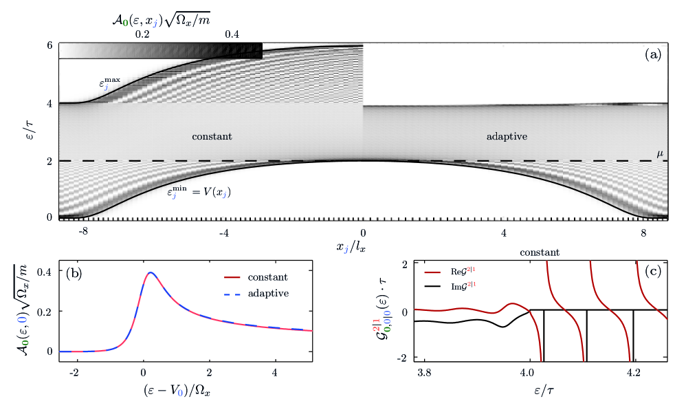
these states are now subject to scattering at the barrier which causes the formation of standing wave patterns for energies $\varepsilon\!<\!V_{{\color[rgb]{0,0,1}0}}=\!V({\color[rgb]{0,0,1}0})\!=\!V_{c}\!+\!\mu$ below the barrier top. The left half ($x_{{\color[rgb]{0,0,1}j}}\!<\!0$) of Fig. 1(a) shows the noninteracting central region’s local density of states (LDOS), $\mathcal{A}_{{\color[rgb]{0,.5,0}\textbf{0}}}^{\sigma}(x_{{\color[rgb]{0,0,1}j}},\varepsilon)\!=\!-1/(\pi a)\!\cdot\!{\rm{Im}}\mathcal{G}_{{\color[rgb]{0,.5,0}\textbf{0}},{\color[rgb]{0,0,1}j}|{\color[rgb]{0,0,1}j}}^{\sigma,{\color[rgb]{1,0,0}2}|{\color[rgb]{1,0,0}1}}(\varepsilon)$ at $B\!=\!0$, as a function of position $x_{{\color[rgb]{0,0,1}j}}$ and energy $\varepsilon$. Due to the condition of adiabaticity the energy band smoothly follows the shape of the potential, implying a site-dependent upper band edge, $\varepsilon^{{\rm{max}}}(x_{{\color[rgb]{0,0,1}j}})\!=\!V_{\color[rgb]{0,0,1}j}\!+4\tau$.

The local maximum of $\varepsilon^{\rm{max}}(x_{{\color[rgb]{0,0,1}j}})$ in the central region’s center generates artificial bound states, owed to the discretization scheme, in the energy interval $\varepsilon\!\in\![4\tau,4\tau+\!V_{{\color[rgb]{0,0,1}0}}]$. This is illustrated in Figure 1(c), where the real and imaginary parts of the bare Green’s function of the central site, $\mathcal{G}_{{\color[rgb]{0,.5,0}\textbf{0}},{\color[rgb]{0,0,1}0}|{\color[rgb]{0,0,1}0}}^{{\color[rgb]{1,0,0}2}|{\color[rgb]{1,0,0}1}}(\varepsilon)$, are plotted. These bound states result from the shape of the upper band edge: Since the band in the homogeneous leads is restricted to energies below $4\tau$ (unlike in the continuous case), all states with higher energy are spacially confined to within the central region, have an infinite lifetime and form a discrete spectrum, determined by the shape of the applied potential $V(x_{{\color[rgb]{0,0,1}j}})$.

The calculation of self-energy and two particle vertex, Eq. (51) and Eq. (45), is performed by ad-infinitum frequency integrations over products of Green’s functions. Thus, the energy region of the upper band edge and the local bound states must be included in their calculation with adequate care. This involves determining the exact position and weigth of the bound states, which requires high numerical effort, as well as dealing with the numerical evaluation of principal value integrals and convolutions, where one function has poles and the other one is continuous. While all this is doable with sufficient dedication, we can avoid such complications entirely by adapting the discretization scheme, discussed next.

V.1.2 Adaptive discretization

According to Eq. (59) and Eq. (60) we can modify the band width locally by choosing non-equidistant discretization points. In the following we discuss a non-constant discretization scheme that reduces the band width within the central region enough so that the upper band edge exhibits a local minimum at $x_{{\color[rgb]{0,0,1}0}}$ rather than a local maximum (as in the case of constant spacing). In consequence the Green’s functions are continuous within the whole energy band, which facilitates a numerical treatment of interactions.

For a non-constant real space discretization it proves useful to first define the onsite energy $E_{{\color[rgb]{0,0,1}j}}$ and the hopping $\tau_{{\color[rgb]{0,0,1}j}}$ of the discrete tight-binding Hamiltonian Eq. (58) and then use these expressions to calculate the geometry of the corresponding physical barrier, i.e. its height $V_{c}$ and curvature $\Omega_{x}$.

We specify the onsite energy to be quadratic near the top with

$\displaystyle E_{\color[rgb]{0,0,1}j}=\tilde{E}_{\color[rgb]{0,0,1}j}+2\tau\simeq\tilde{E}_{\color[rgb]{0,0,1}0}\left[1-\frac{{\color[rgb]{0,0,1}j}^{2}}{N^{\prime 2}}\right]+2\tau,$ (62)

where $\tilde{E}_{{\color[rgb]{0,0,1}0}}$ is positive. We use the shape of $\tilde{E}_{\color[rgb]{0,0,1}j}$ within $C$ (which, apart from its height and the quadratic shape around the top does not influence transport properties, as long as $\tilde{E}_{\color[rgb]{0,0,1}j}$ goes adiabatically to zero upon approaching ${\color[rgb]{0,0,1}j}=|N^{\prime}|$) to define a site-dependent hopping (amounting to a site-dependent spacing)

$\displaystyle\tau_{\color[rgb]{0,0,1}j}=\tau\left[1-\frac{c}{2\tau}\left(\tilde{E}_{\color[rgb]{0,0,1}j}+\tilde{E}_{{\color[rgb]{0,0,1}j+1}}\right)\right],$ (63)

where we have introduced a dimensionless positive parameter $c<\tau/\tilde{E}_{{\color[rgb]{0,0,1}0}}$ that determines how strongly the band width is to be reduced. Note that Eq. (63) describes a hopping, that is constant ($=\tau$) in the leads, where $\tilde{E}_{{\color[rgb]{0,0,1}j}}\!=\!V_{{\color[rgb]{0,0,1}j}}\!=\!0$, and decreases with increasing $\tilde{E}_{{\color[rgb]{0,0,1}j}}$ in the central region. This corresponds to a site-dependent lattice spacing $a_{{\color[rgb]{0,0,1}j}}\!=\!a\sqrt{\tau/\tau_{{\color[rgb]{0,0,1}j}}}$, which increases towards the center of the central region. The real space position $x_{{\color[rgb]{0,0,1}j}}$ that corresponds to a site ${\color[rgb]{0,0,1}j}$ is given by

$\displaystyle x_{{\color[rgb]{0,0,1}j}}=\operatorname{sgn}({\color[rgb]{0,0,1}j})\sum_{{\color[rgb]{0,0,1}j^{\prime}}=1}^{|{\color[rgb]{0,0,1}j}|}a_{{\color[rgb]{0,0,1}j^{\prime}}}=a\sqrt{\tau}\operatorname{sgn}({\color[rgb]{0,0,1}j})\sum_{{\color[rgb]{0,0,1}j^{\prime}}=1}^{|{\color[rgb]{0,0,1}j}|}\frac{1}{\sqrt{\tau_{{\color[rgb]{0,0,1}j}}}},$ (64)

where $\operatorname{sgn}(x)$ is the sign function. Following Eq. (59), the construction introduced in Eq. (62) and Eq. (63) leads to an upper band edge given by

$\displaystyle\varepsilon_{{\color[rgb]{0,0,1}j}}^{\rm{max}}\simeq E_{\color[rgb]{0,0,1}j}+\tau_{{\color[rgb]{0,0,1}j-1}}+\tau_{\color[rgb]{0,0,1}j}\simeq 4\tau+(1-2c)\tilde{E}_{\color[rgb]{0,0,1}j},$ (65)

which for the choice $c\!>\!0.5$ indeed exhibits a smooth local minimum at ${\color[rgb]{0,0,1}j}\!=\!0$, thus avoiding the bound states discussed above for the constant discretization, $c\!=\!0$.

Refer to caption
Figure 2: : (a)-(c), Linear conductance as a function of barrier height $V_{c}$ for some values of magnetic field $B$ with interaction strength $U$ increasing from left to right. (d)-(f), Linear conductance as a function of barrier height $V_{c}$ for some values of temperature $T$ with interaction strength $U$ increasing from left to right. Interactions cause an asymmetric evolution of conductance with magnetic field and temperature due to the interaction-enhanced reduction of conductance in the sub-open regime – the 0.7 anomaly.

Despite the drastic manipulation of $\varepsilon_{{\color[rgb]{0,0,1}j}}^{\rm{max}}$, the lower band edge still serves as a proper potential barrier,

$\displaystyle\varepsilon_{{\color[rgb]{0,0,1}j}}^{\rm{min}}\!=\!V_{\color[rgb]{0,0,1}j}\simeq(1+2c)\tilde{E}_{\color[rgb]{0,0,1}j},$ (66)

with a quadratic potential barrier top whose height now depends on the compensation factor $c$:

$\displaystyle V_{\color[rgb]{0,0,1}j}\simeq(1+2c)\tilde{E}_{\color[rgb]{0,0,1}j}\left[1-\frac{{\color[rgb]{0,0,1}j}^{2}}{N^{\prime 2}}\right].$ (67)

Finally, we write the potential barrier in the form given in Eq. (61), i.e. express the curvature $\Omega_{x}$ in units of the constant lead-hopping $\tau$. By comparison we find

$$V_{c}=V_{{\color[rgb]{0,0,1}0}}-\mu,\qquad\Omega_{x}=\frac{2}{N^{\prime}}\sqrt{V_{{\color[rgb]{0,0,1}0}}\tau_{{\color[rgb]{0,0,1}0}}}.$$ (68)

The right half ($x_{{\color[rgb]{0,0,1}j}}\!>\!0$) of Fig. 1(a) shows the LDOS of the central region for an adaptive discretization with $c\!=\!0.55$. All additional parameters are chosen such that the resulting potential barrier matches the case of constant discretization (plotted for $x_{{\color[rgb]{0,0,1}j}}\!<\!0$). Most importantly, the minimum of $\varepsilon_{{\color[rgb]{0,0,1}j}}^{\rm{max}}$ at ${\color[rgb]{0,0,1}j}\!=\!0$ prevents the occurance of bound states above the barrier, which allows for a faster numerical evaluation of the vertex functions. Importantly, both discretization schemes approximate the same physical system; their differences are non-neglegible only for energies far above the barrier, i.e. far away from the energies relevant for transport. This can be seen from the matching grey scale at the interface ${\color[rgb]{0,0,1}j}\!=\!0$ for energies $\varepsilon<V_{\color[rgb]{0,0,1}0}+\mathcal{O}(\Omega_{x})$, as well as from comparison of the central site’s LDOS in Fig. 1(c).

V.2 The choice of system parameters

To ensure that the discrete model reflects the transport properties of the continuous barrier, Eq. (57), the chemical potential of the system (or of both leads in non-equilibrium) must be chosen far enough below the global minimum of $\varepsilon^{\rm{max}}(x_{{\color[rgb]{0,0,1}j}})$. Only in this case the unphysical upper band edge does not contribute to the results. The onsite-energy is chosen as

$\displaystyle\tilde{E}_{\color[rgb]{0,0,1}j}$ $\displaystyle=\theta(N^{\prime}-|{\color[rgb]{0,0,1}j}|)\tilde{E}_{\color[rgb]{0,0,1}0}\exp\!\left(-\frac{\left(\frac{{\color[rgb]{0,0,1}j}}{N^{\prime}}\right)^{2}}{1-\left(\frac{{\color[rgb]{0,0,1}j}}{N^{\prime}}\right)^{2}}\right),$ (69)

where $\theta(x)$ is the Heavyside step function. Note, that this definition is consistent with Eq. (62). In order to calculate the site-dependent coupling we use $c\!=0.55$ in Eq. (63). Hence, for a barrier height $V_{\color[rgb]{0,0,1}0}\!=\!\mu$ (corresponding to a noninteracting transmission $\mathcal{T}_{{\color[rgb]{0,.5,0}\textbf{0}}}\!=\!0.5$, see Eq. (71) below), we get a potential curvature $\Omega_{x}\!=\!0.039\tau$. Finally, the shape of the onsite interaction is chosen as

$\displaystyle U_{\color[rgb]{0,0,1}j}$ $\displaystyle=\theta(N^{\prime}-|{\color[rgb]{0,0,1}j}|)U_{\color[rgb]{0,0,1}0}\exp\!\left(-\frac{\left(\frac{{\color[rgb]{0,0,1}j}}{N^{\prime}}\right)^{6}}{1-\left(\frac{{\color[rgb]{0,0,1}j}}{N^{\prime}}\right)^{2}}\right).$ (70)

V.3 Non-interacting properties of the model

In Ref. Bauer et al. (2013) we argued that the model of Eq. (58), combined with a potential with parabolic barrier top, Eq. (57), is sufficient to describe the physics of the lowest subband of a QPC: Making a saddle-point ansatz for the electrostatic potential caused by voltages applied to a typical QPC gate structure provides an effective 1D-potential of the form Eq. (57). Information about the transverse geometry of the QPCs potential can be incorporated into the site-dependent effective interaction strength $U_{\color[rgb]{0,0,1}j}$, see Eq. (70).

The non-interacting, spin-dependent transmission through a quadratic barrier of height $V_{{\color[rgb]{0,0,1}0}}=V_{c}+\mu$ and curvature $\Omega_{x}$, Eq. (57), in the presence of a magnetic field $B$ can be derived analytically Büttiker (1990) and is given by

$\displaystyle\mathcal{T}_{{\color[rgb]{0,.5,0}\textbf{0}}}^{\sigma}(\varepsilon)=\frac{1}{e^{-2\pi(\varepsilon-V_{\color[rgb]{0,0,1}0}+\sigma B/2)/\Omega_{x}}+1}.$ (71)

Hence, according to the Landauer-Büttiker formula, the non-interacting (bare) linear conductance,

$\displaystyle\text{g}_{{\color[rgb]{0,.5,0}\textbf{0}}}=-\frac{e^{2}}{h}\sum_{\sigma}\int_{-\infty}^{\infty}f^{\prime}(\varepsilon)\mathcal{T}_{{\color[rgb]{0,.5,0}\textbf{0}}}^{\sigma}(\varepsilon),$ (72)

is a step function of width $\Omega_{x}$ at $B\!=\!T\!=\!0$, changing from 00 to $1$, when the barrier top is shifted through $\mu$ from above. This step gets broadened with temperature [see Figure 2(d)] and develops a double-step structure with magnetic field [see Figure 2(a)]. For all $B$ and $T$ the bare conductance obeys the symmetry $\text{g}_{{\color[rgb]{0,.5,0}\textbf{0}}}(V_{c})=1-\text{g}_{{\color[rgb]{0,.5,0}\textbf{0}}}(-V_{c})$.

Furthermore, an analytic expression for the non-interacting LDOS at the chemical potential in the barrier center as function of barrier height $V_{c}$ can be calculated [see e.g. Ref. Sloggett, C. et al. (2008)],

$\displaystyle\mathcal{A}_{{\color[rgb]{0,.5,0}\textbf{0}}}(\varepsilon\!=\!\mu,{\color[rgb]{0,0,1}0})=\frac{\left|\Gamma\left(1/4+iV_{c}/(2\Omega_{x})\right)\right|^{2}}{4\sqrt{2}\pi^{2}e^{\pi V_{c}/(2\Omega_{x})}},$ (73)

where $\Gamma(z)$ is the complex gamma-function. This is a smeared and shifted version of the 1D van Hove singularity [see Ref. Bauer et al. (2013) for further details], peaked at $V_{c}\!=\!-\mathcal{O}(\Omega_{x})$, i.e. if the barrier top lies sightly below the chemical potential. Here, the value of the noninteracting conductance is given by $\text{g}_{{\color[rgb]{0,.5,0}\textbf{0}}}\approx 0.8$. Hence, we call this parameter regime sub-open.

V.4 Interacting results

As was discussed in Ref. Bauer et al. (2013), the shape of the LDOS in the barrier center lies at the heart of the mechanism causing the 0.7 conductance anomaly: Semiclassically, the LDOS can be interpreted as being inversely proportional to the velocity $v$ of the charge carriers, $\mathcal{A}_{{\color[rgb]{0,.5,0}\textbf{0}}}(\varepsilon,x_{{\color[rgb]{0,0,1}j}})\propto 1/v_{{\color[rgb]{0,0,1}j}}(\varepsilon)$. Hence, the average time that a non-interacting electron with energy $\varepsilon=\mu$ spends in the vicinity of the barrier center is maximal in the sub-open regime (where $\mathcal{A}_{{\color[rgb]{0,.5,0}\textbf{0}}}(\mu,{\color[rgb]{0,0,1}0})$ is maximal, see Eq. (73) and its subsequent discussion), resulting in an enhanced scattering probability and thus a strong reduction of conductance at finite interaction strength in this parameter regime.

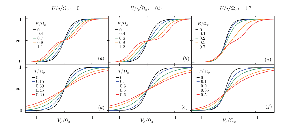
Figure 2 compares the bare conductance, calculated via the Landauer-Büttiker formula [Eq. (72)], with the conductance obtained by taking into account interactions using SOPT, calculated via the Keldysh version of Oguri’s formula [Eq. (26)], as a function of barrier height $V_{c}$ for several values of magnetic field (panels (a)-(c)) and temperature (panels (d)-(f)), for three interaction strengths increasing from left to right. For small but finite interactions, $U\sqrt{\Omega_{x}\tau}=0.5$, the shape of the LDOS causes a slight asymmetry in the conductance curves at (b) finite magnetic field or (e) finite temperature: A finite magnetic field induces an imbalance of spin-species in the vicinity of the barrier center. This imbalance is enhanced by exchange interactions via Stoner-type physics, where the disfavoured spin species (say spin down) is pushed out of the center region by the coulomb blockade of the the favoured spin-species (say spin up). Hence, transport is dominated by the spin-up channel, resulting in a strong reduction of total conductance in the sub-open regime even for a small magnetic field. A finite temperature, on the other hand, opens phase-space for inelastic scattering, which, again, is strongest for large LDOS, again resulting in the reduction of conductance in the sub-open regime. This interaction-induced trend continues with increasing interactions, and gives rise to a weak 0.7 anomaly at $B\neq 0$, Figure 2(c), or $T\neq 0$, Figure 2(f), for intermediate interaction strength, $U\sqrt{\Omega_{x}\tau}=1.7$. Upon a further increase of interactions, SOPT breaks down (see below), and more elaborate methods are needed to obtain qualitatively correct results. This was done in Ref. Bauer et al. (2013) and Ref. Weidinger et al. (2017), where we used fRG to reach interaction strength of up to $U\sqrt{\Omega_{x}\tau}=3.5$; they yielded a pronounced 0.7 anomaly even at $B=T=0$ and its typical magnetic field development into the spin-resolved conductance steps at high field.

The main limitations of SOPT when treating the inhomogeneous system, introduced in Eq. (57), can be explained as follows: Upon increasing interactions, the LDOS is shifted towards higher energy, as Hartree contributions cause an effective higher potential barrier compared to the non-interaction case. As a consequence, a proper description of interactions requires information about this shift to be incorporated into the calculation of the vertex functions via feed-back of the self-energy into all propagators. However, SOPT calculates the self-energy and the two-particle vertex [Section IV] using only bare propagators, which only carry information of the bare LDOS. Together with the drastic truncation of the perturbation series beyond second order, this limits the quantitative validity of SOPT to weak interaction strength and the qualitative validity of SOPT to intermediate interaction strength. In particular, the skewing of the conductance curves with increasing temperature is typically much stronger for measured data curves than seen in Fig. 2(f). Nevertheless, SOPT does serve as a useful too for illustrating the essential physics involved in the appearance of the 0.7 conductance anomaly.

VI Conclusion and Outlook

In this paper we discuss electronic transport through an interacting region of arbitrary shape using the Keldysh formalism. Starting from the well-established Meir-Wingreen formula for the system’s current we derive exact formulas for both the differential and linear conductance. In the latter case we use the fRG flow-equation for the self-energy as well as a Ward identity, following from the Hamiltonian’s particle conservation, to obtain a Keldysh version of Oguri’s linear conductance formula. As an application, we use SOPT to calculate the conductance of the lowest subband of a QPC, which we model by a one-dimensional parabolic potential barrier and onsite interactions – a setup we have recently used to explore the microscopic origin of the 0.7 conductance anomaly Bauer et al. (2013). We present detailed discussion of the model’s properties and argue that an adaptive, non-constant real space discretization scheme greatly facilitates numerical effort. We treat the influence of interactions using SOPT, presenting all details that are necessary to employ the derived conductance formulas. Our SOPT-results for the linear conductance as function of magnetic field and temperature illustrate that the anomalous reduction of conductance in the sub-open regime of a QPC is due to an interplay of the van-Hove ridge and electron-electron interactions.

A logical next step would be to go beyond SOPT by treating interactions using Keldysh-fRG. Work in this direction is currently in progress. For example, in Ref. Schimmel et al. (2017) the conductance formula (26) was used to compute the finite-temperature linear conductance through an interacting QPC using Keldysh-fRG.

Acknowledgements

We thank S. Andergassen, S. Jakobs, V. Meden and H. Schoeller for very helpful discussions. We acknowledge support from the DFG via SFB-631, SFB-TR12, De730/4-3, and the Cluster of Excellence Nanosystems Initiative Munich.

Appendix A Properties of Green’s and vertex functions in Keldysh formalism

To investigate transport properties of the system in and out of equilibrium, we apply the well-established Keldysh formalism Keldysh (1964); Kamenev and Levchenko (2009). Here we collect some of its standard ingredients. We mostly follow the definitions and conventions given in Ref. Jakobs et al. (2010).

All operators carry Keldysh time-contour indices, ${\color[rgb]{1,0,0}a_{1}},{\color[rgb]{1,0,0}a_{1}^{\prime}},{\color[rgb]{1,0,0}a_{2}},...=\{{\color[rgb]{1,0,0}+},{\color[rgb]{1,0,0}-}\}$, marking the position of the time argument $t$ of an operator as lying on the forward (${\color[rgb]{1,0,0}-}$) or backward (+) branch of the Keldysh contour. We use Keldysh indices with or without a prime, ${\color[rgb]{1,0,0}a}$ or ${\color[rgb]{1,0,0}a^{\prime}}$, to label the time arguments of annihilation or creation operators, respectively. Since the model Hamiltonian, Eq. (1), is time-independent, the only non-zero matrix elements of the Hamiltonian in contour space have equal contour indices:

$\displaystyle\mathcal{H}_{{\color[rgb]{0,.5,0}\textbf{0}}}^{{\color[rgb]{1,0,0}a_{1}}|{\color[rgb]{1,0,0}a_{1}^{\prime}}}$ $\displaystyle=-{\color[rgb]{1,0,0}a_{1}}\cdot\delta_{\color[rgb]{1,0,0}a_{1}a_{1}^{\prime}}H_{{\color[rgb]{0,.5,0}\textbf{0}}},$
$\displaystyle\mathcal{H}_{\rm{int}}^{{{\color[rgb]{1,0,0}a_{1}a_{2}}|{\color[rgb]{1,0,0}a_{1}^{\prime}a_{2}^{\prime}}}}$ $\displaystyle=-{\color[rgb]{1,0,0}a_{1}}\cdot\delta_{\color[rgb]{1,0,0}a_{1}a_{2}}\delta_{\color[rgb]{1,0,0}a_{1}a_{1}^{\prime}}\delta_{\color[rgb]{1,0,0}a_{1}a_{2}^{\prime}}H_{\rm{int}},$ (A.1)

with $\{{\color[rgb]{1,0,0}a}\}$ labeling the time arguments of annihilation operators and $\{{\color[rgb]{1,0,0}a^{\prime}}\}$ labeling the time arguments of creation operators. Note that a calligraphic $\mathcal{H}$ carries contour indices, while a capital $H$ does not.

We define time-dependent, $n$-particle Keldysh Green’s functions as the expectation values

$\displaystyle G_{\mbox{\scriptsize{\boldmath${\color[rgb]{0,0,1}i}$}}|\mbox{\scriptsize{\boldmath${\color[rgb]{0,0,1}i^{\prime}}$}}}^{n,\mbox{\scriptsize{\boldmath${\color[rgb]{1,0,0}a}$}}|\mbox{\scriptsize{\boldmath${\color[rgb]{1,0,0}a^{\prime}}$}}\mbox{\boldmath{}}}(\mbox{\normalsize{\boldmath$t$}}|\mbox{\normalsize{\boldmath$t^{\prime}$}}\mbox{\boldmath{}})=G_{{\color[rgb]{0,0,1}i_{1}},...,{\color[rgb]{0,0,1}i_{n}}|{\color[rgb]{0,0,1}i_{1}^{\prime}},...{\color[rgb]{0,0,1}i_{n}^{\prime}}}^{{\color[rgb]{1,0,0}a_{1}},...,{\color[rgb]{1,0,0}a_{n}}|{\color[rgb]{1,0,0}a_{1}^{\prime}},...{\color[rgb]{1,0,0}a_{n}^{\prime}}}(t_{1},...,t_{n}|t_{n}^{\prime},...,t_{1}^{\prime})=$
$\displaystyle(-i)^{n}\langle\mathcal{T}_{c}d_{{\color[rgb]{0,0,1}i_{1}}}^{\color[rgb]{1,0,0}a_{1}}(t_{1})...d_{{\color[rgb]{0,0,1}i_{n}}}^{\color[rgb]{1,0,0}a_{n}}(t_{n})[d_{{\color[rgb]{0,0,1}i_{n}^{\prime}}}^{\color[rgb]{1,0,0}a_{n}^{\prime}}]^{\dagger}(t_{n}^{\prime})...[d_{{\color[rgb]{0,0,1}i_{1}^{\prime}}}^{\color[rgb]{1,0,0}a_{1}^{\prime}}]^{\dagger}(t_{1}^{\prime})\rangle,$ (A.2)

where we use boldface notation for multi-indices $\mbox{\boldmath{$x$}}=(x_{1},...,x_{n})$. The operator $d_{{\color[rgb]{0,0,1}i}}^{{\color[rgb]{1,0,0}a}}(t)/\left[d_{{\color[rgb]{0,0,1}i}}^{{\color[rgb]{1,0,0}a}}\right]^{\dagger}\!(t)$ destroys/creates an electron at time $t$ on contour branch ${\color[rgb]{1,0,0}a}$ in quantum state ${\color[rgb]{0,0,1}i}$, and the time-ordering operator $\mathcal{T}_{c}$ moves later contour times to the left. In case of equal time arguments, annihilation operators are always arranged to the right of creation operators. The bare, non-interacting Green’s function, whose time-dependence is governed by the quadratic part of the Hamiltonian, $\mathcal{H}_{{\color[rgb]{0,.5,0}\textbf{0}}}$, carries an additional subscript, $G_{{\color[rgb]{0,.5,0}\textbf{0}}}$.

We define anti-symmetrized, irreducible, $n$-particle vertex functions, $\gamma_{\mbox{\scriptsize{\boldmath${\color[rgb]{0,0,1}i^{\prime}}$}}|\mbox{\scriptsize{\boldmath${\color[rgb]{0,0,1}i}$}}}^{n,\mbox{\scriptsize{\boldmath${\color[rgb]{1,0,0}a^{\prime}}$}}|\mbox{\scriptsize{\boldmath${\color[rgb]{1,0,0}a}$}}\mbox{\boldmath{}}}(\mbox{\normalsize{\boldmath$t^{\prime}$}}|\mbox{\normalsize{\boldmath$t$}}\mbox{\boldmath{}})$, as the sum of all $1$-particle irreducible ($1$PI) diagrams with $n$ amputated ingoing and $n$ amputated outgoing legs. For an explicit series representation of the one- and two-particle vertex, see Eq. (B.1). A formula for the prefactor of every single diagram is given by Eq. (20) of Ref. Jakobs et al. (2010).

The Dyson equation provides a direct relation between the one-particle Green’s and vertex function:

$$G(t_{1}|t_{1}^{\prime})\!=\!G_{{\color[rgb]{0,.5,0}\textbf{0}}}(t_{1}|t_{1}^{\prime})\!-\!\int\!d\tau_{1}d\tau_{1}^{\prime}G_{{\color[rgb]{0,.5,0}\textbf{0}}}(t_{1}|\tau_{1}^{\prime})\gamma(\tau_{1}^{\prime}|\tau_{1})G(\tau_{1}|t_{1}^{\prime}).$$ (A.3)

Here and below, whenever quantum state indices ${\color[rgb]{0,0,1}i}$ and contour indices ${\color[rgb]{1,0,0}a}$/Keldysh indices ${\color[rgb]{1,0,0}\alpha}$ are implicit, they are understood to be summed over in products.

Decomposing the two-particle Green’s yields a connection to the two-particle vertex function via

$\displaystyle G(t_{1},t_{2}|t_{1}^{\prime},t_{2}^{\prime})=G(t_{1}|t_{1}^{\prime})G(t_{2}|t_{2}^{\prime})-G(t_{1}|t_{2}^{\prime})G(t_{2}|t_{1}^{\prime})$
$\displaystyle-\!i\!\int\!d\mbox{\boldmath$\tau$}G(t_{1}|\tau_{1}^{\prime})G(t_{2}|\tau_{2}^{\prime})\gamma(\tau_{1}^{\prime},\tau_{2}^{\prime}|\tau_{1},\tau_{2})G(\tau_{1}|t_{1}^{\prime})G(\tau_{2}|t_{2}^{\prime}).$ (A.4)

Our choice of sign for $\gamma$ is opposite to that of Ref. Jakobs et al. (2010).

Since the Hamiltonian, Eq. (1), is time-independent, the Green’s/vertex functions are translationally invariant in time, implying that $n$-particle functions depend on $2n-1$ time arguments only:

$\displaystyle G(t_{1},...,t_{n}|t_{1}^{\prime},...t_{n}^{\prime})$ $\displaystyle=G(0,...,t_{n}-t_{1}|t_{1}^{\prime}-t_{1},...,t_{n}^{\prime}-t_{1}),$
$\displaystyle\gamma(t_{1}^{\prime},...,t_{n}^{\prime}|t_{1},...t_{n})$ $\displaystyle=\gamma(0,...,t_{n}^{\prime}-t_{1}^{\prime}|t_{1}-t_{1}^{\prime},...,t_{n}-t_{1}^{\prime}).$ (A.5)

As a consequence, the Fourier-transform,

$\displaystyle G(\mbox{\normalsize{\boldmath$\varepsilon$}}|\mbox{\normalsize{\boldmath$\varepsilon^{\prime}$}}\mbox{\boldmath{}})$ $\displaystyle=\int\!d\mathbf{t}d\mathbf{t^{\prime}}\leavevmode\nobreak\ e^{i\mbox{\footnotesize{\boldmath$\varepsilon t$}}\mbox{\boldmath{}}}e^{-i\mbox{\footnotesize{\boldmath$\varepsilon^{\prime}t^{\prime}$}}\mbox{\boldmath{}}}G(\mathbf{t}|\mathbf{t^{\prime}}),$
$\displaystyle\gamma(\mbox{\normalsize{\boldmath$\varepsilon^{\prime}$}}|\mbox{\normalsize{\boldmath$\varepsilon$}}\mbox{\boldmath{}})$ $\displaystyle=\int\!d\mathbf{t}d\mathbf{t^{\prime}}\leavevmode\nobreak\ e^{i\mbox{\footnotesize{\boldmath$\varepsilon^{\prime}t^{\prime}$}}\mbox{\boldmath{}}}e^{-i\mbox{\footnotesize{\boldmath$\varepsilon t$}}\mbox{\boldmath{}}}\gamma(\mathbf{t^{\prime}}|\mathbf{t}),$ (A.6)

fulfills energy conservation. In particular, this allows for the following representation for the one- and two-particle functions, where calligraphic letters $\mathcal{G}$ and $\mathcal{L}$ are used when a $\delta$-function has been split off:

$\displaystyle G(\varepsilon_{1}|\varepsilon_{1}^{\prime})=2\pi\delta(\varepsilon_{1}-\varepsilon_{1}^{\prime})\mathcal{G}(\varepsilon_{1}),$
$\displaystyle G(\varepsilon_{1},\varepsilon_{2}|\varepsilon_{1}^{\prime},\varepsilon_{2}^{\prime})=2\pi\delta(\varepsilon_{1}+\varepsilon_{2}-\varepsilon_{1}^{\prime}-\varepsilon_{2}^{\prime})\mathcal{G}(\varepsilon_{2},\varepsilon_{1}^{\prime};\varepsilon_{1}-\varepsilon_{1}^{\prime}),$
$\displaystyle\gamma(\varepsilon_{1}^{\prime}|\varepsilon_{1})=-2\pi\delta(\varepsilon_{1}^{\prime}-\varepsilon_{1})\Sigma(\varepsilon_{1}^{\prime}),$
$\displaystyle\gamma(\varepsilon_{1}^{\prime},\varepsilon_{2}^{\prime}|\varepsilon_{1},\varepsilon_{2})=2\pi\delta(\varepsilon_{1}^{\prime}+\varepsilon_{2}^{\prime}-\varepsilon_{1}-\varepsilon_{2})\mathcal{L}(\varepsilon_{2}^{\prime},\varepsilon_{1};\varepsilon_{1}^{\prime}-\varepsilon_{1}).$ (A.7)

The one-particle vertex-function $\Sigma$, introduced above, is called the interacting irreducible self-energy. We Fourier-transform Dyson’s equation, Eq. (A.3), which provides

$\displaystyle\mathcal{G}(\varepsilon)\!$ $\displaystyle=\!\mathcal{G}_{{\color[rgb]{0,.5,0}\textbf{0}}}(\varepsilon)\!+\!\mathcal{G}_{{\color[rgb]{0,.5,0}\textbf{0}}}(\varepsilon)\Sigma(\varepsilon)\mathcal{G}(\varepsilon)\!=\!\left[\left[\mathcal{G}_{{\color[rgb]{0,.5,0}\textbf{0}}}(\varepsilon)\right]^{-1}-\Sigma(\varepsilon)\right]^{-1}.$ (A.8)

Note that this is a matrix equation in both Keldysh and position space.

The four single-particle Green’s functions and self-energies in contour space are called chronological ($\mathcal{G}^{{\color[rgb]{1,0,0}-|-}}$, $\Sigma^{{\color[rgb]{1,0,0}-|-}}$), lesser ($\mathcal{G}^{{\color[rgb]{1,0,0}-|+}}$, $\Sigma^{{\color[rgb]{1,0,0}-|+}}$), greater ($\mathcal{G}^{{\color[rgb]{1,0,0}+|-}}$, $\Sigma^{{\color[rgb]{1,0,0}+|-}}$) and anti-chronological ($\mathcal{G}^{{\color[rgb]{1,0,0}+|+}}$, $\Sigma^{{\color[rgb]{1,0,0}+|+}}$). As a consequence of the definition, Eq. (A.2), the single-particle Green’s functions fulfill the contour-relation

$$\mathcal{G}^{{\color[rgb]{1,0,0}+}|{\color[rgb]{1,0,0}+}}+\mathcal{G}^{{\color[rgb]{1,0,0}-}|{\color[rgb]{1,0,0}-}}=\mathcal{G}^{{\color[rgb]{1,0,0}-}|{\color[rgb]{1,0,0}+}}+\mathcal{G}^{{\color[rgb]{1,0,0}+}|{\color[rgb]{1,0,0}-}}.$$ (A.9)

We define the transformation from contour space (${\color[rgb]{1,0,0}a}=\{{\color[rgb]{1,0,0}-},{\color[rgb]{1,0,0}+}\}$) into Keldysh space (${\color[rgb]{1,0,0}\alpha}=\{{\color[rgb]{1,0,0}1},{\color[rgb]{1,0,0}2}\}$) by the rotation

$\displaystyle R=\left(\begin{array}[]{cc}R^{{\color[rgb]{1,0,0}-}|{\color[rgb]{1,0,0}1}}&R^{{\color[rgb]{1,0,0}-}|{\color[rgb]{1,0,0}2}}\\ R^{{\color[rgb]{1,0,0}+}|{\color[rgb]{1,0,0}1}}&R^{{\color[rgb]{1,0,0}+}|{\color[rgb]{1,0,0}2}}\end{array}\right)=\frac{1}{\sqrt{2}}\left(\begin{array}[]{cc}1&1\\ -1&1\end{array}\right).$ (A.14)

Hence, any $n$-th rank tensor $A^{n,{\color[rgb]{1,0,0}\mbox{\scriptsize{\boldmath$\alpha^{\prime}$}}}|\mbox{\scriptsize{\boldmath${\color[rgb]{1,0,0}\alpha}$}}\mbox{\boldmath{}}}$ in Keldysh space is represented in contour space by

$\displaystyle A^{n,\mbox{\scriptsize{\boldmath${\color[rgb]{1,0,0}\alpha}$}}|\mbox{\scriptsize{\boldmath${\color[rgb]{1,0,0}\alpha^{\prime}}$}}\mbox{\boldmath{}}}=\sum_{\mbox{\scriptsize{\boldmath${\color[rgb]{1,0,0}a}$}},\mbox{\scriptsize{\boldmath${\color[rgb]{1,0,0}a^{\prime}}$}}\mbox{\boldmath{}}}\left[R^{-1}\right]^{\mbox{\scriptsize{\boldmath${\color[rgb]{1,0,0}\alpha}$}}|\mbox{\scriptsize{\boldmath${\color[rgb]{1,0,0}a}$}}\mbox{\boldmath{}}}A^{n,\mbox{\scriptsize{\boldmath${\color[rgb]{1,0,0}a}$}}|\mbox{\scriptsize{\boldmath${\color[rgb]{1,0,0}a^{\prime}}$}}\mbox{\boldmath{}}}R^{\mbox{\scriptsize{\boldmath${\color[rgb]{1,0,0}a^{\prime}}$}}|\mbox{\scriptsize{\boldmath${\color[rgb]{1,0,0}\alpha^{\prime}}$}}\mbox{\boldmath{}}}.$ (A.15)

As can be shown explicitly (see Chapter 4.3 of Ref. Jakobs et al. (2010)) the Green’s and vertex functions fulfill a theorem of causality:

$\displaystyle\mathcal{G}^{{{\color[rgb]{1,0,0}1}...{\color[rgb]{1,0,0}1}|{\color[rgb]{1,0,0}1}...{\color[rgb]{1,0,0}1}}}=0,$
$\displaystyle\mathcal{L}^{{{\color[rgb]{1,0,0}2}...{\color[rgb]{1,0,0}2}|{\color[rgb]{1,0,0}2}...{\color[rgb]{1,0,0}2}}}=0.$ (A.16)

The remaining three non-zero Keldysh components of the single-particle functions are called retarded ($\mathcal{G}^{{\color[rgb]{1,0,0}2}|{\color[rgb]{1,0,0}1}}$, $\Sigma^{{\color[rgb]{1,0,0}1}|{\color[rgb]{1,0,0}2}}$), advanced ($\mathcal{G}^{{\color[rgb]{1,0,0}1}|{\color[rgb]{1,0,0}2}}$, $\Sigma^{{\color[rgb]{1,0,0}2}|{\color[rgb]{1,0,0}1}}$) and Keldysh ($\mathcal{G}^{{\color[rgb]{1,0,0}2}|{\color[rgb]{1,0,0}2}}$, $\Sigma^{{\color[rgb]{1,0,0}1}|{\color[rgb]{1,0,0}1}}$):

$\displaystyle\mathcal{G}$ $\displaystyle=\left(\begin{array}[]{cc}0&\mathcal{G}^{{\color[rgb]{1,0,0}A}}\\ \mathcal{G}^{{\color[rgb]{1,0,0}R}}&\mathcal{G}^{{\color[rgb]{1,0,0}K}}\end{array}\right)=\left(\begin{array}[]{cc}0&\mathcal{G}^{{\color[rgb]{1,0,0}1}|{\color[rgb]{1,0,0}2}}\\ \mathcal{G}^{{\color[rgb]{1,0,0}2}|{\color[rgb]{1,0,0}1}}&\mathcal{G}^{{\color[rgb]{1,0,0}2}|{\color[rgb]{1,0,0}2}}\end{array}\right),$ (A.21)
$\displaystyle\Sigma$ $\displaystyle=\left(\begin{array}[]{cc}\Sigma^{{\color[rgb]{1,0,0}K}}&\Sigma^{{\color[rgb]{1,0,0}R}}\\ \Sigma^{{\color[rgb]{1,0,0}A}}&0\end{array}\right)=\left(\begin{array}[]{cc}\Sigma^{{\color[rgb]{1,0,0}1}|{\color[rgb]{1,0,0}1}}&\Sigma^{{\color[rgb]{1,0,0}1}|{\color[rgb]{1,0,0}2}}\\ \Sigma^{{\color[rgb]{1,0,0}2}|{\color[rgb]{1,0,0}1}}&0\end{array}\right).$ (A.26)

The transformation, Eq. (A.15), provides the identities

$\displaystyle\mathcal{G}^{{{\color[rgb]{1,0,0}-}}|{{\color[rgb]{1,0,0}+}}}$ $\displaystyle=\frac{1}{2}\left[\mathcal{G}^{{{\color[rgb]{1,0,0}2}|{\color[rgb]{1,0,0}2}}}-\left(\mathcal{G}^{{{\color[rgb]{1,0,0}2}|{\color[rgb]{1,0,0}1}}}-\mathcal{G}^{{{\color[rgb]{1,0,0}1}|{\color[rgb]{1,0,0}2}}}\right)\right],$ (A.27a)
$\displaystyle\mathcal{G}^{{{\color[rgb]{1,0,0}+}}|{{\color[rgb]{1,0,0}-}}}-\mathcal{G}^{{{\color[rgb]{1,0,0}-}}|{{\color[rgb]{1,0,0}+}}}$ $\displaystyle=\mathcal{G}^{{{\color[rgb]{1,0,0}2}|{\color[rgb]{1,0,0}1}}}-\mathcal{G}^{{{\color[rgb]{1,0,0}1}|{\color[rgb]{1,0,0}2}}},$ (A.27b)
$\displaystyle\mathcal{H}_{{\color[rgb]{0,.5,0}\textbf{0}}}^{{\color[rgb]{1,0,0}1}|{\color[rgb]{1,0,0}2}}$ $\displaystyle=\mathcal{H}_{{\color[rgb]{0,.5,0}\textbf{0}}}^{{\color[rgb]{1,0,0}2}|{\color[rgb]{1,0,0}1}}=H_{{\color[rgb]{0,.5,0}\textbf{0}}}\leavevmode\nobreak\ ,\leavevmode\nobreak\ \mathcal{H}_{{\color[rgb]{0,.5,0}\textbf{0}}}^{{\color[rgb]{1,0,0}1}|{\color[rgb]{1,0,0}1}}=\mathcal{H}_{{\color[rgb]{0,.5,0}\textbf{0}}}^{{\color[rgb]{1,0,0}2}|{\color[rgb]{1,0,0}2}}=0,$ (A.27c)

all of which are used in the derivation of the conductance formula in Sec. I. Note that a calligraphic $\mathcal{H}$ carries Keldysh indices, while a capital $H$ does not. The retarded/advanced components are analytic in the upper/lower half plane of the complex frequency plane. Hence, the following notation is always implied,

$\displaystyle\mathcal{G}^{{\color[rgb]{1,0,0}2}|{\color[rgb]{1,0,0}1}}(\varepsilon)$ $\displaystyle=\mathcal{G}^{{\color[rgb]{1,0,0}2}|{\color[rgb]{1,0,0}1}}(\varepsilon+i\delta)\leavevmode\nobreak\ ,\leavevmode\nobreak\ \Sigma^{{\color[rgb]{1,0,0}1}|{\color[rgb]{1,0,0}2}}(\varepsilon)=\Sigma^{{\color[rgb]{1,0,0}1}|{\color[rgb]{1,0,0}2}}(\varepsilon+i\delta),$ (A.28)
$\displaystyle\mathcal{G}^{{\color[rgb]{1,0,0}1}|{\color[rgb]{1,0,0}2}}(\varepsilon)$ $\displaystyle=\mathcal{G}^{{\color[rgb]{1,0,0}1}|{\color[rgb]{1,0,0}2}}(\varepsilon-i\delta)\leavevmode\nobreak\ ,\leavevmode\nobreak\ \Sigma^{{\color[rgb]{1,0,0}2}|{\color[rgb]{1,0,0}1}}(\varepsilon)=\Sigma^{{\color[rgb]{1,0,0}2}|{\color[rgb]{1,0,0}1}}(\varepsilon-i\delta),$ (A.29)

with real, infinitesimal, positive $\delta$. In contrast, the Keldysh component describes fluctuations, restricted to the real frequency axis. In equilibrium, the single-particle functions fulfill a fluctuation dissipation theorem (FDT):

$\displaystyle\Sigma^{{\color[rgb]{1,0,0}1}|{\color[rgb]{1,0,0}1}}(\varepsilon)=(1-2f(\varepsilon))\big{[}\Sigma^{{\color[rgb]{1,0,0}1}|{\color[rgb]{1,0,0}2}}(\varepsilon)-\Sigma^{{\color[rgb]{1,0,0}2}|{\color[rgb]{1,0,0}1}}(\varepsilon)\big{]},$ (A.30a)
$\displaystyle\mathcal{G}^{{\color[rgb]{1,0,0}2}|{\color[rgb]{1,0,0}2}}(\varepsilon)=(1-2f(\varepsilon))\big{[}\mathcal{G}^{{\color[rgb]{1,0,0}2}|{\color[rgb]{1,0,0}1}}(\varepsilon)-\mathcal{G}^{{\color[rgb]{1,0,0}1}|{\color[rgb]{1,0,0}2}}(\varepsilon)\big{]},$ (A.30b)

where $f(\varepsilon)=1/(1+\exp[(\varepsilon-\mu)/T])$ is the Fermi distribution function.

Within this work we consider a system composed of a finite central interacting region coupled to two non-interacting fermionic leads: The left lead, with chemical potential $\mu_{L}$ and temperature $T_{L}$, and the right lead, with chemical potential $\mu_{R}$ and temperature $T_{R}$. We can represent the quadratic part of the Hamiltonian in block-matrix form as

$\displaystyle{h}_{{\color[rgb]{0,.5,0}\textbf{0}}}\!=\!\left(\begin{array}[]{ccc}h_{l}&h_{lc}&0\\ \leavevmode\nobreak\ \!\!h_{cl}&h_{{\color[rgb]{0,.5,0}\textbf{0}},c}&h_{cr}\\ 0&h_{rc}&h_{r}\\ \end{array}\right).$ (A.34)

where the matrices $h_{l}$ and $h_{r}$ fully define the properties of the isolated leads, and the matrix $h_{{\color[rgb]{0,.5,0}\textbf{0}},c}$ describes the non-interacting part of the isolated central region. Finally, $h_{cl}$ and $h_{cr}$ specify the coupling of the central region to the corresponding lead. Similarly, we write the system’s Green’s function, $\mathcal{G}(\varepsilon)$ [Eq. (A.8)], in the same basis (for the bare, non-interacting Green’s function $\mathcal{G}_{{\color[rgb]{0,.5,0}\textbf{0}}}$ we set $\Sigma\!=\!0$):

$\displaystyle\mathcal{G}\!=\!\left(\begin{array}[]{ccc}\mathcal{G}_{l}&\mathcal{G}_{lc}&\mathcal{G}_{lr}\\ \mathcal{G}_{cl}&\mathcal{G}_{c}&\mathcal{G}_{cr}\\ \mathcal{G}_{rl}&\mathcal{G}_{rc}&\mathcal{G}_{r}\\ \end{array}\right).$ (A.38)

We use the small letter $g$ to denote the Green’s function of an isolated subsystem, e.g. $g_{l}(\varepsilon)$ is the Green’s function of the isolated left lead $L$. The non-interacting Green’s function of the central region is given by Dyson’s equation

$\displaystyle\mathcal{G}_{{\color[rgb]{0,.5,0}\textbf{0}},c}$ $\displaystyle=g_{{\color[rgb]{0,.5,0}\textbf{0}},c}\!+\!g_{{\color[rgb]{0,.5,0}\textbf{0}},c}\Sigma_{{\rm{lead}}}\mathcal{G}_{{\color[rgb]{0,.5,0}\textbf{0}},c}=\left[\left[g_{{\color[rgb]{0,.5,0}\textbf{0}},c}\right]^{-1}\!-\!\Sigma_{{\rm{lead}}}\right]^{-1}.$ (A.39)

Again note that this is a matrix equation in Keldysh and position space. We incorporated environment contributions into the lead self-energy

$\displaystyle\Sigma_{{\rm{lead}}}=\sum_{k=l,r}h_{ck}g_{k}h_{kc}.$ (A.40)

The individual Keldysh components of the non-interacting Green’s function are given by

$\displaystyle\mathcal{G}_{{\color[rgb]{0,.5,0}\textbf{0}},c}^{{\color[rgb]{1,0,0}1}|{\color[rgb]{1,0,0}2}}(\varepsilon)$ $\displaystyle=\left(\varepsilon-h_{c}-\Sigma_{{\rm{lead}}}^{{\color[rgb]{1,0,0}2}|{\color[rgb]{1,0,0}1}}(\varepsilon)\right)^{-1},$ (A.41a)
$\displaystyle\mathcal{G}_{{\color[rgb]{0,.5,0}\textbf{0}},c}^{{\color[rgb]{1,0,0}2}|{\color[rgb]{1,0,0}1}}(\varepsilon)$ $\displaystyle=\left(\varepsilon-h_{c}-\Sigma_{{\rm{lead}}}^{{\color[rgb]{1,0,0}1}|{\color[rgb]{1,0,0}2}}(\varepsilon)\right)^{-1},$ (A.41b)
$\displaystyle\mathcal{G}_{{\color[rgb]{0,.5,0}\textbf{0}},c}^{{\color[rgb]{1,0,0}2}|{\color[rgb]{1,0,0}2}}(\varepsilon)$ $\displaystyle=\mathcal{G}_{{\color[rgb]{0,.5,0}\textbf{0}},c}^{{\color[rgb]{1,0,0}2}|{\color[rgb]{1,0,0}1}}(\varepsilon)\Sigma_{{\rm{lead}}}^{{\color[rgb]{1,0,0}1}|{\color[rgb]{1,0,0}1}}(\varepsilon)\mathcal{G}_{{\color[rgb]{0,.5,0}\textbf{0}},c}^{{\color[rgb]{1,0,0}1}|{\color[rgb]{1,0,0}2}}(\varepsilon)$
$\displaystyle=-i\sum_{k=l,r}[1-2f^{k}(\varepsilon)]\mathcal{G}_{{\color[rgb]{0,.5,0}\textbf{0}},c}^{{\color[rgb]{1,0,0}2}|{\color[rgb]{1,0,0}1}}(\varepsilon)\Gamma^{k}(\varepsilon)\mathcal{G}_{{\color[rgb]{0,.5,0}\textbf{0}},c}^{{\color[rgb]{1,0,0}2}|{\color[rgb]{1,0,0}1}}(\varepsilon),$ (A.41c)

where we introduced the hybridization function, $\Gamma^{k}(\varepsilon)\!=\!ih_{ck}(g_{k}^{{\color[rgb]{1,0,0}2}|{\color[rgb]{1,0,0}1}}(\varepsilon)\!-\!g_{k}^{{\color[rgb]{1,0,0}1}|{\color[rgb]{1,0,0}2}}(\varepsilon))h_{kc}$.

With the interaction being restricted to the central region we use the notation $\Sigma=\Sigma_{c}=C\Sigma C$ for the interacting self-energy. Dyson’s equation, Eq. (A.8), and the real space structure, Eq. (A.38), yields

$\displaystyle\mathcal{G}_{c}(\varepsilon)=\left[\left[\mathcal{G}_{{\color[rgb]{0,.5,0}\textbf{0}},c}(\varepsilon)\right]^{-1}-\Sigma(\varepsilon)\right]^{-1}.$ (A.42)

The matrix representation of its Keldysh structure is given by

$\displaystyle\left(\begin{array}[]{cc}0&\mathcal{G}_{c}^{{\color[rgb]{1,0,0}1}|{\color[rgb]{1,0,0}2}}\\ \mathcal{G}_{c}^{{\color[rgb]{1,0,0}2}|{\color[rgb]{1,0,0}1}}&\mathcal{G}_{c}^{{\color[rgb]{1,0,0}2}|{\color[rgb]{1,0,0}2}}\\ \end{array}\right)\!=\!\left[\left(\begin{array}[]{cc}0&\mathcal{G}_{{\color[rgb]{0,.5,0}\textbf{0}},c}^{{\color[rgb]{1,0,0}1}|{\color[rgb]{1,0,0}2}}\\ \mathcal{G}_{{\color[rgb]{0,.5,0}\textbf{0}},c}^{{\color[rgb]{1,0,0}2}|{\color[rgb]{1,0,0}1}}&\mathcal{G}_{{\color[rgb]{0,.5,0}\textbf{0}},c}^{{\color[rgb]{1,0,0}2}|{\color[rgb]{1,0,0}2}}\\ \end{array}\right)^{-1}-\left(\begin{array}[]{cc}\Sigma^{{\color[rgb]{1,0,0}1}|{\color[rgb]{1,0,0}1}}&\Sigma^{{\color[rgb]{1,0,0}1}|{\color[rgb]{1,0,0}2}}\\ \Sigma^{{\color[rgb]{1,0,0}2}|{\color[rgb]{1,0,0}1}}&0\\ \end{array}\right)\right]^{-1}.$ (A.49)

Block matrix inversion then provides the components

$\displaystyle\mathcal{G}_{c}^{{\color[rgb]{1,0,0}1}|{\color[rgb]{1,0,0}2}}(\varepsilon)$ $\displaystyle=\left(\varepsilon-h_{c}-\Sigma_{{\rm{lead}}}^{{\color[rgb]{1,0,0}2}|{\color[rgb]{1,0,0}1}}(\varepsilon)-\Sigma^{{\color[rgb]{1,0,0}2}|{\color[rgb]{1,0,0}1}}(\varepsilon)\right)^{-1},$ (A.50a)
$\displaystyle\mathcal{G}_{c}^{{\color[rgb]{1,0,0}2}|{\color[rgb]{1,0,0}1}}(\varepsilon)$ $\displaystyle=\left(\varepsilon-h_{c}-\Sigma_{{\rm{lead}}}^{{\color[rgb]{1,0,0}1}|{\color[rgb]{1,0,0}2}}(\varepsilon)-\Sigma^{{\color[rgb]{1,0,0}1}|{\color[rgb]{1,0,0}2}}(\varepsilon)\right)^{-1},$ (A.50b)
$\displaystyle\mathcal{G}_{c}^{{\color[rgb]{1,0,0}2}|{\color[rgb]{1,0,0}2}}(\varepsilon)$ $\displaystyle=\mathcal{G}_{c}^{{\color[rgb]{1,0,0}2}|{\color[rgb]{1,0,0}1}}(\varepsilon)\left[\Sigma_{{\rm{lead}}}^{{\color[rgb]{1,0,0}1}|{\color[rgb]{1,0,0}1}}+\Sigma^{{\color[rgb]{1,0,0}1}|{\color[rgb]{1,0,0}1}}\right]\mathcal{G}_{c}^{{\color[rgb]{1,0,0}1}|{\color[rgb]{1,0,0}2}}(\varepsilon).$ (A.50c)

From Eq. (A.8), we can show, that the off-diagonal components of the full Green’s function, are given by

$\displaystyle\mathcal{G}_{kc}=g_{k}\mathcal{H}_{kc}\mathcal{G}_{c}\leavevmode\nobreak\ ,\leavevmode\nobreak\ \mathcal{G}_{ck}=\mathcal{G}_{c}\mathcal{H}_{ck}g_{k},$ (A.51)

where in this single case, $\mathcal{H}_{kc}$ is the matrix-element $h_{kc}$ with additional Keldysh-structure. In general, one has

$\displaystyle\mathcal{G}_{{\color[rgb]{0,.5,0}\textbf{0}},{\color[rgb]{0,0,1}i}|{\color[rgb]{0,0,1}j}}^{{\color[rgb]{1,0,0}1}|{\color[rgb]{1,0,0}2}}$ $\displaystyle\!=\!\left[\mathcal{G}_{{\color[rgb]{0,.5,0}\textbf{0}},{\color[rgb]{0,0,1}j}|{\color[rgb]{0,0,1}i}}^{{\color[rgb]{1,0,0}2}|{\color[rgb]{1,0,0}1}}\right]^{*}\!,\mathcal{G}_{{\color[rgb]{0,0,1}i}|{\color[rgb]{0,0,1}j}}^{{\color[rgb]{1,0,0}1}|{\color[rgb]{1,0,0}2}}\!=\!\left[\mathcal{G}_{{\color[rgb]{0,0,1}j}|{\color[rgb]{0,0,1}i}}^{{\color[rgb]{1,0,0}2}|{\color[rgb]{1,0,0}1}}\right]^{*}\!,\Sigma_{{\color[rgb]{0,0,1}i}|{\color[rgb]{0,0,1}j}}^{{\color[rgb]{1,0,0}1}|{\color[rgb]{1,0,0}2}}\!=\!\left[\Sigma_{{\color[rgb]{0,0,1}j}|{\color[rgb]{0,0,1}i}}^{{\color[rgb]{1,0,0}2}|{\color[rgb]{1,0,0}1}}\right]^{*}\!,$ (A.52a)
$\displaystyle\mathcal{G}_{{\color[rgb]{0,.5,0}\textbf{0}},{\color[rgb]{0,0,1}i}|{\color[rgb]{0,0,1}j}}^{{\color[rgb]{1,0,0}2}|{\color[rgb]{1,0,0}2}}$ $\displaystyle\!=\!-\left[\mathcal{G}_{{\color[rgb]{0,.5,0}\textbf{0}},{\color[rgb]{0,0,1}j}|{\color[rgb]{0,0,1}i}}^{{\color[rgb]{1,0,0}2}|{\color[rgb]{1,0,0}2}}\right]^{*}\!,\mathcal{G}_{{\color[rgb]{0,0,1}i}|{\color[rgb]{0,0,1}j}}^{{\color[rgb]{1,0,0}2}|{\color[rgb]{1,0,0}2}}\!=\!-\left[\mathcal{G}_{{\color[rgb]{0,0,1}j}|{\color[rgb]{0,0,1}i}}^{{\color[rgb]{1,0,0}2}|{\color[rgb]{1,0,0}2}}\right]^{*}\!,\Sigma_{{\color[rgb]{0,0,1}i}|{\color[rgb]{0,0,1}j}}^{{\color[rgb]{1,0,0}1}|{\color[rgb]{1,0,0}1}}\!=\!-\left[\Sigma_{{\color[rgb]{0,0,1}j}|{\color[rgb]{0,0,1}i}}^{{\color[rgb]{1,0,0}1}|{\color[rgb]{1,0,0}1}}\right]^{*}.$ (A.52b)

For a symmetric, real Hamiltonian, the following additional symmetries hold in equilibrium

$\displaystyle\mathcal{G}_{{\color[rgb]{0,.5,0}\textbf{0}},{\color[rgb]{0,0,1}i}|{\color[rgb]{0,0,1}j}}^{{\color[rgb]{1,0,0}1}|{\color[rgb]{1,0,0}2}}$ $\displaystyle\!=\!\mathcal{G}_{{\color[rgb]{0,.5,0}\textbf{0}},{\color[rgb]{0,0,1}j}|{\color[rgb]{0,0,1}i}}^{{\color[rgb]{1,0,0}1}|{\color[rgb]{1,0,0}2}}\leavevmode\nobreak\ ,\leavevmode\nobreak\ \mathcal{G}_{{\color[rgb]{0,0,1}i}|{\color[rgb]{0,0,1}j}}^{{\color[rgb]{1,0,0}1}|{\color[rgb]{1,0,0}2}}\!=\!\mathcal{G}_{{\color[rgb]{0,0,1}j}|{\color[rgb]{0,0,1}i}}^{{\color[rgb]{1,0,0}1}|{\color[rgb]{1,0,0}2}}\leavevmode\nobreak\ ,\leavevmode\nobreak\ \Sigma_{{\color[rgb]{0,0,1}i}|{\color[rgb]{0,0,1}j}}^{{\color[rgb]{1,0,0}1}|{\color[rgb]{1,0,0}2}}\!=\!\Sigma_{{\color[rgb]{0,0,1}j}|{\color[rgb]{0,0,1}i}}^{{\color[rgb]{1,0,0}1}|{\color[rgb]{1,0,0}2}},$ (A.53a)
$\displaystyle\mathcal{G}_{{\color[rgb]{0,.5,0}\textbf{0}},{\color[rgb]{0,0,1}i}|{\color[rgb]{0,0,1}j}}^{{\color[rgb]{1,0,0}2}|{\color[rgb]{1,0,0}1}}$ $\displaystyle\!=\!\mathcal{G}_{{\color[rgb]{0,.5,0}\textbf{0}},{\color[rgb]{0,0,1}j}|{\color[rgb]{0,0,1}i}}^{{\color[rgb]{1,0,0}2}|{\color[rgb]{1,0,0}1}}\leavevmode\nobreak\ ,\leavevmode\nobreak\ \mathcal{G}_{{\color[rgb]{0,0,1}i}|{\color[rgb]{0,0,1}j}}^{{\color[rgb]{1,0,0}2}|{\color[rgb]{1,0,0}1}}\!=\!\mathcal{G}_{{\color[rgb]{0,0,1}j}|{\color[rgb]{0,0,1}i}}^{{\color[rgb]{1,0,0}2}|{\color[rgb]{1,0,0}1}}\leavevmode\nobreak\ ,\leavevmode\nobreak\ \Sigma_{{\color[rgb]{0,0,1}i}|{\color[rgb]{0,0,1}j}}^{{\color[rgb]{1,0,0}2}|{\color[rgb]{1,0,0}1}}\!=\!\Sigma_{{\color[rgb]{0,0,1}j}|{\color[rgb]{0,0,1}i}}^{{\color[rgb]{1,0,0}2}|{\color[rgb]{1,0,0}1}}.$ (A.53b)

Appendix B   Diagrammatic discussion of the fRG flow-equation of the self-energy

In this appendix we provide a diagrammatic plausibility argument for the fRG flow-equation for the self-energy, Eq. (16). A detailed diagrammatic derivation may be found in Ref. Jakobs et al. (2007b). We use the observation, that every diagram in the diagrammatic series of the self-energy contains a sub-diagram which appears in the diagrammatic series of the two-particle vertex. As a consequence, taking the derivative of the self-energy, $\partial_{\Lambda}\Sigma$, w.r.t. some parameter $\Lambda$ allows for a resummation of diagrams, such that the full two-particle vertex series can be factorized. Hence, we get an equation which can formally be written as $\partial_{\Lambda}\Sigma_{\Lambda}=\int\!S_{\Lambda}\mathcal{L}_{\Lambda}$, with the socalled single-scale propagator $S$ and the two-particle vertex $\mathcal{L}$, both depending on the parameter $\Lambda$.

The self-energy $\Sigma$ and two-particle vertex $\mathcal{L}$ are diagrammatically defined as the sum of all one-particle irreducible diagrams with two and four amputated external legs, respectively. Using the graphical representation of the bare Green’s function, Eq. (30), and the bare vertex, Eq. (34), the first terms of their perturbation series are (we omit the arrows for the sake of simplicity)

[Uncaptioned image]matrix[Uncaptioned image]\displaystyle\begin{matrix}\includegraphics[width=455.24408pt]{Sigma_series_noarrows.pdf}\end{matrix} (B.1a)
[Uncaptioned image]matrix[Uncaptioned image]\displaystyle\begin{matrix}\includegraphics[width=455.24408pt]{Gamma_series.pdf}\end{matrix} (B.1b)

We introduce a parameter $\Lambda$ into the bare propagator, $\mathcal{G}_{{\color[rgb]{0,.5,0}\textbf{0}}}\rightarrow\mathcal{G}_{{\color[rgb]{0,.5,0}\textbf{0}}}^{\Lambda}$, and represent its derivative w.r.t. $\Lambda$ by a crossed-out line, Λ𝒢0Λ=[Uncaptioned image].subscriptΛsuperscriptsubscript𝒢0Λmatrix[Uncaptioned image]\partial_{\Lambda}\mathcal{G}_{{\color[rgb]{0,.5,0}\textbf{0}}}^{\Lambda}=\begin{matrix}\includegraphics[width=28.45274pt]{G_cutoff.pdf}\end{matrix}. Hence, the derivative of the self-energy is given by

[Uncaptioned image]matrix[Uncaptioned image]\displaystyle\begin{matrix}\includegraphics[width=512.1496pt]{Sigma_series_derivative.pdf}\end{matrix} (B.2)

where we introduced the socalled single scale propagator

$\displaystyle\phantom{S_{\Lambda}}=\left[1+\mathcal{G}_{{\color[rgb]{0,.5,0}\textbf{0}}}\Sigma+\mathcal{G}_{{\color[rgb]{0,.5,0}\textbf{0}}}\Sigma\mathcal{G}_{{\color[rgb]{0,.5,0}\textbf{0}}}\Sigma+\dots\right]\left(\partial_{\Lambda}\mathcal{G}_{{\color[rgb]{0,.5,0}\textbf{0}}}^{\Lambda}\Sigma\right)\left[1+\mathcal{G}_{{\color[rgb]{0,.5,0}\textbf{0}}}\Sigma+\mathcal{G}_{{\color[rgb]{0,.5,0}\textbf{0}}}\Sigma\mathcal{G}_{{\color[rgb]{0,.5,0}\textbf{0}}}\Sigma+\dots\right]$
$\displaystyle\phantom{S_{\Lambda}}=\mathcal{G}\left[\mathcal{G}_{{\color[rgb]{0,.5,0}\textbf{0}}}\right]^{-1}\left(\partial_{\Lambda}\mathcal{G}_{{\color[rgb]{0,.5,0}\textbf{0}}}^{\Lambda}\Sigma\right)\left[\mathcal{G}_{{\color[rgb]{0,.5,0}\textbf{0}}}\right]^{-1}\mathcal{G}$ (B.3)

Finally, we fix the prefactor of the diagram on the r.h.s. in Eq. (B.2) by the following argument: The first order self-energy, $\Sigma_{{\color[rgb]{0,.5,0}\textbf{1}}}$, is of Hartree-type and hence purely determined by the local density $n_{{\color[rgb]{0,0,1}j}}$ and the local interaction strength $U_{{\color[rgb]{0,0,1}j}}$. We calculate the first order self-energy in equilibrium

$\displaystyle\left.\Sigma^{R}_{{\color[rgb]{0,.5,0}\textbf{1}},{\color[rgb]{0,0,1}j}}\right|_{V=0}=n_{{\color[rgb]{0,0,1}j}}U_{{\color[rgb]{0,0,1}j}}=\frac{1}{\pi i}\bar{u}_{{\color[rgb]{0,0,1}j}}\int d\varepsilon\leavevmode\nobreak\ \mathcal{G}_{{\color[rgb]{0,.5,0}\textbf{0}},{\color[rgb]{0,0,1}j}|{\color[rgb]{0,0,1}j}}^{<}(\varepsilon).$ (B.4)

The derivative of Eq. (B.4) is given by

$\displaystyle\left.\partial_{\Lambda}\Sigma^{R}_{{\color[rgb]{0,.5,0}\textbf{1}},{\color[rgb]{0,0,1}j}}\right|_{V=0}=\frac{1}{2\pi i}\bar{u}_{{\color[rgb]{0,0,1}j}}\int d\varepsilon\leavevmode\nobreak\ \partial_{\Lambda}\left(\mathcal{G}_{{\color[rgb]{0,.5,0}\textbf{0}},{\color[rgb]{0,0,1}j}|{\color[rgb]{0,0,1}j}}^{K}(\varepsilon)+\mathcal{G}_{{\color[rgb]{0,.5,0}\textbf{0}},{\color[rgb]{0,0,1}j}|{\color[rgb]{0,0,1}j}}^{A}(\varepsilon)-\mathcal{G}_{{\color[rgb]{0,.5,0}\textbf{0}},{\color[rgb]{0,0,1}j}|{\color[rgb]{0,0,1}j}}^{R}(\varepsilon)\right).$ (B.5)

$G^{R}$ is analytic in the upper half plane. For reasonable flow parameters (in particular flow parameters associated with a physical quantity, like temperature or source-drain bias), $\partial_{\Lambda}G^{R}$ is also analytic in the upper half plane and $\partial_{\Lambda}G^{R}$ decays sufficiently fast as function of energy that the contour may be closed in the lower half-plane to yield zero. For analogous reasons, $\partial_{\Lambda}G^{A}$ yields zero, too. Therefore, Eq. (B.5) simplifies to

$\displaystyle\left.\partial_{\Lambda}\Sigma^{R}_{{\color[rgb]{0,.5,0}\textbf{1}},{\color[rgb]{0,0,1}j}}\right|_{V=0}=\frac{1}{2\pi i}\bar{u}_{{\color[rgb]{0,0,1}j}}\int d\varepsilon\leavevmode\nobreak\ \partial_{\Lambda}\mathcal{G}_{{\color[rgb]{0,.5,0}\textbf{0}},{\color[rgb]{0,0,1}j}|{\color[rgb]{0,0,1}j}}^{K}(\varepsilon),$ (B.6)

which fixes the prefactor of the diagram on the r.h.s. in Eq. (B.2). Hence, we end up with Eq. (16) for the derivative of the self-energy:

$\displaystyle\partial_{\Lambda}\Sigma_{{\color[rgb]{0,0,1}i}|{\color[rgb]{0,0,1}j}}^{{\color[rgb]{1,0,0}\alpha^{\prime}}|{\color[rgb]{1,0,0}\alpha}}(\varepsilon)=\frac{1}{2\pi i}\int d\varepsilon^{\prime}\sum_{\underset{{\color[rgb]{0,0,1}kl}\in C}{{\color[rgb]{1,0,0}\beta\beta^{\prime}}}}S_{\Lambda,{\color[rgb]{0,0,1}k}|{\color[rgb]{0,0,1}l}}^{{\color[rgb]{1,0,0}\beta}|{\color[rgb]{1,0,0}\beta^{\prime}}}(\varepsilon^{\prime})\mathcal{L}_{{\color[rgb]{0,0,1}ik}|{\color[rgb]{0,0,1}jl}}^{{\color[rgb]{1,0,0}\alpha^{\prime}\beta^{\prime}}|{\color[rgb]{1,0,0}\alpha\beta}}(\varepsilon^{\prime},\varepsilon;0).$ (B.7)

Appendix C   Charge conservation - Ward identity

In this Appendix we derive the Ward identity used in the main text, Eq. (24), from variational principles, following Ref. Zinn-Justin (1993). Since the action corresponding to the Hamiltonian, Eq. (1), is invariant under a global $U(1)$ symmetry, it satisfies a conservation law. Starting from the path integral representation of expectation values using Grassmann variables, the requirement of vanishing variation under the gauged $U(1)$ transformation yields both a continuity equation for particle current and the desired connection between the interacting self-energy $\Sigma$, introduced in Eq. (A.7), and the vertex part $\Phi$, defined in Eq. (23).

Within this Appendix, for notational convenience, we combine the left and right lead, thus representing the matrix $h$ in the Hamiltonian Eq. (1) and the Green’s function by

$\displaystyle h=\left(\begin{array}[]{cc}h_{c}&h_{c\ell}\\ \leavevmode\nobreak\ \!\!h_{\ell c}&h_{\ell}\end{array}\right)\leavevmode\nobreak\ ,\leavevmode\nobreak\ \mathcal{G}=\left(\begin{array}[]{cc}\mathcal{G}_{c}&\mathcal{G}_{c\ell}\\ \mathcal{G}_{\ell c}&\mathcal{G}_{\ell}\end{array}\right),$ (C.5)

where $l$ corresponds to spatial indices in either lead, and $c$ to spatial indices within the central region. Let $\{\psi\},\{\bar{\psi}\}$ be sets of Grassmann variables, i.e. fermionic fields. We write $n$-particle expectation values in terms of the functional path integral,

$\displaystyle G_{\mbox{\scriptsize{\boldmath${\color[rgb]{0,0,1}i}$}}|\mbox{\scriptsize{\boldmath${\color[rgb]{0,0,1}i^{\prime}}$}}}^{n,\mbox{\scriptsize{\boldmath${\color[rgb]{1,0,0}a}$}}|\mbox{\scriptsize{\boldmath${\color[rgb]{1,0,0}a^{\prime}}$}}\mbox{\boldmath{}}}(\mbox{\normalsize{\boldmath$t$}}|\mbox{\normalsize{\boldmath$t^{\prime}$}}\mbox{\boldmath{}})\!=\!(-i)^{n}\langle\psi_{{\color[rgb]{0,0,1}i_{1}}}^{{\color[rgb]{1,0,0}a_{1}}}(t_{1})...\psi_{{\color[rgb]{0,0,1}i_{n}}}^{{\color[rgb]{1,0,0}a_{n}}}(t_{n})\bar{\psi}_{{\color[rgb]{0,0,1}i_{n}^{\prime}}}^{{\color[rgb]{1,0,0}a_{n}^{\prime}}}(t_{n}^{\prime})...\bar{\psi}_{{\color[rgb]{0,0,1}i_{1}^{\prime}}}^{{\color[rgb]{1,0,0}a_{1}^{\prime}}}(t_{1}^{\prime})\rangle\!=\!(-i)^{n}\int\!\mathcal{D}(\mbox{\normalsize{\boldmath$\bar{\psi}$}}\mbox{\normalsize{\boldmath$\psi$}})\psi_{{\color[rgb]{0,0,1}i_{1}}}^{{\color[rgb]{1,0,0}a_{1}}}(t_{1})...\psi_{{\color[rgb]{0,0,1}i_{n}}}^{{\color[rgb]{1,0,0}a_{n}}}(t_{n})\bar{\psi}_{{\color[rgb]{0,0,1}i_{n}^{\prime}}}^{{\color[rgb]{1,0,0}a_{n}^{\prime}}}(t_{n}^{\prime})...\bar{\psi}_{{\color[rgb]{0,0,1}i_{1}^{\prime}}}^{{\color[rgb]{1,0,0}a_{1}^{\prime}}}(t_{1}^{\prime})e^{iS[\mbox{\normalsize{\boldmath$\bar{\psi}$}},\mbox{\normalsize{\boldmath$\psi$}}]},$ (C.6)

where the Keldysh action is given by the Keldysh contour time integral

$\displaystyle S[\mbox{\normalsize{\boldmath$\bar{\psi}$}},\mbox{\normalsize{\boldmath$\psi$}}]\!$ $\displaystyle=\!\int_{\mathcal{C}}dt\sum_{{\color[rgb]{0,0,1}ii^{\prime}}}\bar{\psi}_{{\color[rgb]{0,0,1}i^{\prime}}}(t)(\overbrace{i\delta_{{\color[rgb]{0,0,1}i^{\prime}i}}\partial_{t}-h_{{\color[rgb]{0,0,1}i^{\prime}i}})}^{[G_{{\color[rgb]{0,.5,0}\textbf{0}}}(t)^{-1}]_{{\color[rgb]{0,0,1}i^{\prime}i}}}\psi_{{\color[rgb]{0,0,1}i}}(t)+S_{{\rm{int}}}[\mbox{\normalsize{\boldmath$\bar{\psi}$}},\mbox{\normalsize{\boldmath$\psi$}}]\!=\!\int_{-\infty}^{\infty}dt\sum_{{\color[rgb]{1,0,0}a},{\color[rgb]{0,0,1}ii^{\prime}}}(-{\color[rgb]{1,0,0}a})\bar{\psi}_{{\color[rgb]{0,0,1}i^{\prime}}}^{{\color[rgb]{1,0,0}a}}(t)\left(i\delta_{{\color[rgb]{0,0,1}i^{\prime}i}}\partial_{t}-h_{{\color[rgb]{0,0,1}i^{\prime}i}}\right)\psi_{{\color[rgb]{0,0,1}i}}^{{\color[rgb]{1,0,0}a}}(t)+S_{{\rm{int}}}[\mbox{\normalsize{\boldmath$\bar{\psi}$}},\mbox{\normalsize{\boldmath$\psi$}}]$
$\displaystyle=\int_{-\infty}^{\infty}dt\sum_{{\color[rgb]{1,0,0}a}}(-{\color[rgb]{1,0,0}a})\mbox{\normalsize{\boldmath$\bar{\psi}$}}^{{\color[rgb]{1,0,0}a}}\!(t)\!\left(i\mbox{\normalsize{\boldmath$\partial$}}_{t}-h\right)\mbox{\normalsize{\boldmath$\psi$}}^{{\color[rgb]{1,0,0}a}}(t)+S_{{\rm{int}}}[\mbox{\normalsize{\boldmath$\bar{\psi}$}},\mbox{\normalsize{\boldmath$\psi$}}].$ (C.7)

In the last line we introduced the vector notation $\mbox{\normalsize{\boldmath$\psi$}}\!=\!\left(\!\begin{array}[]{c}\psi_{{\color[rgb]{0,0,1}1}}\\ \psi_{{\color[rgb]{0,0,1}2}}\\ \vdots\\ \end{array}\!\right)$ and $\mbox{\normalsize{\boldmath$\bar{\psi}$}}\!=\!\left(\psi_{{\color[rgb]{0,0,1}1}},\psi_{{\color[rgb]{0,0,1}2}},\ldots\right)$. Note that $\mbox{\normalsize{\boldmath$\partial$}}_{t}$ is a diagonal matrix.

C.1 Gauge transformation

The action, Eq. (C.7), is invariant under the global $U(1)$ transformation $\mbox{\normalsize{\boldmath$\psi$}}\rightarrow\mbox{\normalsize{\boldmath$\psi$}}e^{i\alpha}$ and $\mbox{\normalsize{\boldmath$\bar{\psi}$}}\rightarrow\mbox{\normalsize{\boldmath$\bar{\psi}$}}e^{-i\alpha}$, where $\alpha$ is a real constant. Gauging this transformation, i.e. making $\alpha$ space-, and time-dependent, yields to linear order in $\alpha$

$\displaystyle\delta\psi_{{\color[rgb]{0,0,1}i}}^{{\color[rgb]{1,0,0}a}}(t)=i\alpha_{{\color[rgb]{0,0,1}i}}^{{\color[rgb]{1,0,0}a}}(t)\psi_{{\color[rgb]{0,0,1}i}}^{{\color[rgb]{1,0,0}a}}(t)\leavevmode\nobreak\ ,\leavevmode\nobreak\ \delta\bar{\psi}_{{\color[rgb]{0,0,1}i^{\prime}}}^{{\color[rgb]{1,0,0}a}}(t^{\prime})=-i\alpha_{{\color[rgb]{0,0,1}i^{\prime}}}^{{\color[rgb]{1,0,0}a}}(t^{\prime})\bar{\psi}_{{\color[rgb]{0,0,1}i^{\prime}}}^{{\color[rgb]{1,0,0}a}}(t^{\prime}).$ (C.8)

Since we are interested in the current through the system, from one lead to another, it is convenient to pick $\alpha$ non-vanishing only in the central region:

$\displaystyle\alpha_{{\color[rgb]{0,0,1}i}}^{{\color[rgb]{1,0,0}a}}(t)=\begin{cases}\alpha^{{\color[rgb]{1,0,0}a}}(t),\quad{\rm{if}}\quad{\color[rgb]{0,0,1}i}\in C\\ 0,\quad\hskip 18.00005pt{\rm{if}}\quad{\color[rgb]{0,0,1}i}\in\mathbb{L}.\end{cases}$ (C.9)

This is equivalent to first deriving the Ward identity using an arbitrary $\alpha$ and then summing over the central region. The requirement that the right-hand side of Eq. (C.6) is invariant when applying the gauged $U(1)$ transformation to all $\psi$’s therein now reads:

$$\delta G_{\mbox{\scriptsize{\boldmath${\color[rgb]{0,0,1}i}$}}|\mbox{\scriptsize{\boldmath${\color[rgb]{0,0,1}i^{\prime}}$}}}^{n,\mbox{\scriptsize{\boldmath${\color[rgb]{1,0,0}a}$}}|\mbox{\scriptsize{\boldmath${\color[rgb]{1,0,0}a^{\prime}}$}}\mbox{\boldmath{}}}(\mbox{\normalsize{\boldmath$t$}}|\mbox{\normalsize{\boldmath$t^{\prime}$}}\mbox{\boldmath{}})=0.$$ (C.10)

This requirement is simply a change of the integration variable in field space. In other words, the physical correlators cannot depend on an arbitrary choice of basis in which the fields are represented.

C.2 The continuity equation (zeroth order Ward identity)

For $n=0$, Eq. (C.10) sets a condition on the variation of the partition sum. Since the measure of the path integral is invariant under the transformation in Eq. (C.8) (the $U(1)$-symmetry is not anomalous), this in turn sets a condition on the variation of the action:

$\displaystyle 0=\delta\left[\int\!\mathcal{D}(\mbox{\normalsize{\boldmath$\bar{\psi}$}}\mbox{\normalsize{\boldmath$\psi$}})e^{iS[\mbox{\normalsize{\boldmath$\bar{\psi}$}},\mbox{\normalsize{\boldmath$\psi$}}]}\right]=i\int\!\mathcal{D}(\mbox{\normalsize{\boldmath$\bar{\psi}$}}\mbox{\normalsize{\boldmath$\psi$}})\delta S[\mbox{\normalsize{\boldmath$\bar{\psi}$}},\mbox{\normalsize{\boldmath$\psi$}}]e^{iS[\mbox{\normalsize{\boldmath$\bar{\psi}$}},\mbox{\normalsize{\boldmath$\psi$}}]}.$ (C.11)

The quartic term, $S_{{\rm{int}}}$, describes a density-density interaction. Hence, its variation vanishes trivially and the variation of the total action reduces to the variation of the quadratic term:

$\displaystyle\delta S[\mbox{\normalsize{\boldmath$\bar{\psi}$}},\mbox{\normalsize{\boldmath$\psi$}}]$ $\displaystyle=\int_{-\infty}^{\infty}dt\sum_{{\color[rgb]{1,0,0}a},{\color[rgb]{0,0,1}i}}(-{\color[rgb]{1,0,0}a})\Big{[}\alpha_{{\color[rgb]{0,0,1}i}}^{{\color[rgb]{1,0,0}a}}(t)\bar{\psi}_{{\color[rgb]{0,0,1}i}}^{{\color[rgb]{1,0,0}a}}(t)\partial_{t}\psi_{{\color[rgb]{0,0,1}i}}^{{\color[rgb]{1,0,0}a}}(t)-\bar{\psi}_{{\color[rgb]{0,0,1}i}}^{{\color[rgb]{1,0,0}a}}(t)\partial_{t}\!\left(\alpha_{{\color[rgb]{0,0,1}i}}^{{\color[rgb]{1,0,0}a}}(t)\psi_{{\color[rgb]{0,0,1}i}}^{{\color[rgb]{1,0,0}a}}(t)\right)+\sum_{{\color[rgb]{0,0,1}i^{\prime}}}\big{[}i\alpha_{{\color[rgb]{0,0,1}i^{\prime}}}^{{\color[rgb]{1,0,0}a}}(t)-i\alpha_{{\color[rgb]{0,0,1}i}}^{{\color[rgb]{1,0,0}a}}(t)\big{]}\bar{\psi}_{{\color[rgb]{0,0,1}i^{\prime}}}^{{\color[rgb]{1,0,0}a}}\!(t)h_{{\color[rgb]{0,0,1}i^{\prime}i}}\psi_{{\color[rgb]{0,0,1}i}}^{{\color[rgb]{1,0,0}a}}(t)\Big{]}$
$\displaystyle=\int_{-\infty}^{\infty}dt\sum_{{\color[rgb]{1,0,0}a}}(-{\color[rgb]{1,0,0}a})\alpha^{{\color[rgb]{1,0,0}a}}(t)\Big{[}\partial_{t}\!\left(\mbox{\normalsize{\boldmath$\bar{\psi}$}}_{c}^{{\color[rgb]{1,0,0}a}}(t)\mbox{\normalsize{\boldmath$\psi$}}_{c}^{{\color[rgb]{1,0,0}a}}(t)\right)-i\mbox{\normalsize{\boldmath$\bar{\psi}$}}_{c}^{{\color[rgb]{1,0,0}a}}(t)h_{cl}\mbox{\normalsize{\boldmath$\psi$}}_{l}^{{\color[rgb]{1,0,0}a}}(t)+i\mbox{\normalsize{\boldmath$\bar{\psi}$}}_{l}^{{\color[rgb]{1,0,0}a}}(t)h_{lc}\mbox{\normalsize{\boldmath$\psi$}}_{c}^{{\color[rgb]{1,0,0}a}}(t)\Big{]}$
$\displaystyle=\int_{-\infty}^{\infty}dt\sum_{{\color[rgb]{1,0,0}a}}(-{\color[rgb]{1,0,0}a})\alpha^{{\color[rgb]{1,0,0}a}}(t)\Big{[}-\partial_{t}\!\left(\mbox{\normalsize{\boldmath$\psi$}}_{c}^{{\color[rgb]{1,0,0}a}}(t)\mbox{\normalsize{\boldmath$\bar{\psi}$}}_{c}^{{\color[rgb]{1,0,0}a}}(t)\right)+i{\rm{Tr}}\!\left\{\!h_{cl}\mbox{\normalsize{\boldmath$\psi$}}_{l}^{{\color[rgb]{1,0,0}a}}(t)\mbox{\normalsize{\boldmath$\bar{\psi}$}}_{c}^{{\color[rgb]{1,0,0}a}}(t)\!\right\}-i{\rm{Tr}}\!\left\{\!h_{lc}\mbox{\normalsize{\boldmath$\psi$}}_{c}^{{\color[rgb]{1,0,0}a}}(t)\mbox{\normalsize{\boldmath$\bar{\psi}$}}_{l}^{{\color[rgb]{1,0,0}a}}(t)\!\right\}\Big{]},$ (C.12)

where we used integration by parts in the first term Since Eq. (C.11) must hold for arbitrary $\alpha(t)$ this provides the continuity equation

$\displaystyle-\partial_{t}\langle\mbox{\normalsize{\boldmath$\psi$}}_{c}^{{\color[rgb]{1,0,0}a}}(t)\mbox{\normalsize{\boldmath$\bar{\psi}$}}_{c}^{{\color[rgb]{1,0,0}a}}(t)\rangle=i{\rm{Tr}}\!\left\{\!h_{lc}\langle\mbox{\normalsize{\boldmath$\psi$}}_{c}^{{\color[rgb]{1,0,0}a}}(t)\mbox{\normalsize{\boldmath$\bar{\psi}$}}_{l}^{{\color[rgb]{1,0,0}a}}(t)\rangle\!\right\}-i{\rm{Tr}}\!\left\{\!h_{cl}\langle\mbox{\normalsize{\boldmath$\psi$}}_{l}^{{\color[rgb]{1,0,0}a}}(t)\mbox{\normalsize{\boldmath$\bar{\psi}$}}_{c}^{{\color[rgb]{1,0,0}a}}(t)\rangle\!\right\}.$ (C.13)

In steady-state, the time derivative of the density term on the l.h.s. vanishes and Eq. (C.13) reduces to current conservation, i.e. the current into the central region equals the current out of the central region:

$\displaystyle{\rm{Tr}}\big{\{}\!h_{lc}G_{cl}^{{\color[rgb]{1,0,0}-}|{\color[rgb]{1,0,0}+}}(0)\!\big{\}}={\rm{Tr}}\big{\{}\!h_{cl}G_{lc}^{{\color[rgb]{1,0,0}-}|{\color[rgb]{1,0,0}+}}(0)\!\big{\}}.$ (C.14)

Here we made use of the time-translational invariance of the Green’s function, Eq. (A.5), and the equivalence of the contour Green’s function components for equal-time arguments $G^{{\color[rgb]{1,0,0}-}|{\color[rgb]{1,0,0}+}}(t,t)\!=\!G^{{\color[rgb]{1,0,0}-}|{\color[rgb]{1,0,0}-}}(t,t)\!=\!G^{{\color[rgb]{1,0,0}+}|{\color[rgb]{1,0,0}+}}(t,t)$.

C.3 Relation between self-energy and two-particle vertex (first order Ward identity)

For $n=1$, Eq. (C.10) reads

$\displaystyle 0=\delta\langle\psi_{{\color[rgb]{0,0,1}i}}^{{\color[rgb]{1,0,0}a}}(t)\bar{\psi}_{{\color[rgb]{0,0,1}i^{\prime}}}^{{\color[rgb]{1,0,0}a^{\prime}}}\!(t^{\prime})\rangle=\int\!\mathcal{D}(\mbox{\normalsize{\boldmath$\bar{\psi}$}}\mbox{\normalsize{\boldmath$\psi$}})\left[\left(\delta\psi_{{\color[rgb]{0,0,1}i}}^{{\color[rgb]{1,0,0}a}}(t)\right)\bar{\psi}_{{\color[rgb]{0,0,1}i^{\prime}}}^{{\color[rgb]{1,0,0}a^{\prime}}}(t^{\prime})+\psi_{{\color[rgb]{0,0,1}i}}^{{\color[rgb]{1,0,0}a}}(t)(\delta\bar{\psi}_{{\color[rgb]{0,0,1}i^{\prime}}}^{{\color[rgb]{1,0,0}a^{\prime}}}(t^{\prime}))+i\psi_{{\color[rgb]{0,0,1}i}}^{{\color[rgb]{1,0,0}a}}(t)\bar{\psi}_{{\color[rgb]{0,0,1}i^{\prime}}}^{{\color[rgb]{1,0,0}a^{\prime}}}\!(t^{\prime})(\delta S[\mbox{\normalsize{\boldmath$\bar{\psi}$}},\mbox{\normalsize{\boldmath$\psi$}}])\right]e^{iS[\mbox{\normalsize{\boldmath$\bar{\psi}$}},\mbox{\normalsize{\boldmath$\psi$}}]}.$ (C.15)

Since the r.h.s. contains both terms quadratic and quartic in $\psi$, this equation will eventually lead to a relation between the self-energy and the two-particle vertex. For states ${\color[rgb]{0,0,1}i},{\color[rgb]{0,0,1}i^{\prime}}\!\in\!C$ Eq. (C.15) can be written as

$\displaystyle 0=\int_{\infty}^{\infty}dt^{\prime\prime}\sum_{{\color[rgb]{1,0,0}a^{\prime\prime}}}(-{\color[rgb]{1,0,0}a^{\prime\prime}})i\alpha^{{\color[rgb]{1,0,0}a^{\prime\prime}}}(t^{\prime\prime})\Bigg{\{}$ $\displaystyle\int\!\mathcal{D}(\mbox{\normalsize{\boldmath$\bar{\psi}$}}\mbox{\normalsize{\boldmath$\psi$}})\psi_{{\color[rgb]{0,0,1}i}}^{{\color[rgb]{1,0,0}a}}(t)\bar{\psi}_{{\color[rgb]{0,0,1}i^{\prime}}}^{{\color[rgb]{1,0,0}a^{\prime}}}(t^{\prime})\bigg{[}(-{\color[rgb]{1,0,0}a})\delta(t^{\prime\prime}-t)\delta_{{\color[rgb]{1,0,0}aa^{\prime\prime}}}+{\color[rgb]{1,0,0}a^{\prime}}\delta(t^{\prime\prime}-t^{\prime})\delta_{{\color[rgb]{1,0,0}a^{\prime}a^{\prime\prime}}}$
$\displaystyle\left.+\sum_{{\color[rgb]{0,0,1}j}\in C}\partial_{t^{\prime\prime}}\left(\bar{\psi}_{{\color[rgb]{0,0,1}j}}^{{\color[rgb]{1,0,0}a^{\prime\prime}}}(t^{\prime\prime})\psi_{{\color[rgb]{0,0,1}j}}^{{\color[rgb]{1,0,0}a^{\prime\prime}}}(t^{\prime\prime})\right)\right.$
$\displaystyle+i\sum_{{\color[rgb]{0,0,1}j_{1}},{\color[rgb]{0,0,1}j_{2}}}\left(\bar{\psi}_{{\color[rgb]{0,0,1}j_{1}}}^{{\color[rgb]{1,0,0}a^{\prime\prime}}}(t^{\prime\prime})h_{\ell c,{\color[rgb]{0,0,1}j_{1}}|{\color[rgb]{0,0,1}j_{2}}}\psi_{{\color[rgb]{0,0,1}j_{2}}}^{{\color[rgb]{1,0,0}a^{\prime\prime}}}(t^{\prime\prime})-\bar{\psi}_{{\color[rgb]{0,0,1}j_{2}}}^{{\color[rgb]{1,0,0}a^{\prime\prime}}}(t^{\prime\prime})h_{c\ell,{\color[rgb]{0,0,1}j_{2}}|{\color[rgb]{0,0,1}j_{1}}}\psi_{{\color[rgb]{0,0,1}j_{1}}}^{{\color[rgb]{1,0,0}a^{\prime\prime}}}(t^{\prime\prime})\right)\bigg{]}\!e^{iS[\mbox{\normalsize{\boldmath$\bar{\psi}$}},\mbox{\normalsize{\boldmath$\psi$}}]}\Bigg{\}}.$ (C.16)

Again, this must be true for arbitrary $\alpha(t)$, providing

$\displaystyle\left[(-{\color[rgb]{1,0,0}a})\delta(t^{\prime\prime}-t)\delta_{{\color[rgb]{1,0,0}aa^{\prime\prime}}}+{\color[rgb]{1,0,0}a^{\prime}}\delta(t^{\prime\prime}-t^{\prime})\delta_{{\color[rgb]{1,0,0}a^{\prime}a^{\prime\prime}}}\right]G_{{\color[rgb]{0,0,1}i}|{\color[rgb]{0,0,1}i^{\prime}}}^{{\color[rgb]{1,0,0}a}|{\color[rgb]{1,0,0}a^{\prime}}}(t|t^{\prime})$
$\displaystyle=\sum_{{\color[rgb]{0,0,1}j_{1}},{\color[rgb]{0,0,1}j_{2}}}\left[h_{\ell c,{\color[rgb]{0,0,1}j_{1}}|{\color[rgb]{0,0,1}j_{2}}}G_{{\color[rgb]{0,0,1}j_{2}i}|{\color[rgb]{0,0,1}j_{1}i^{\prime}}}^{{\color[rgb]{1,0,0}a^{\prime\prime}a}|{\color[rgb]{1,0,0}a^{\prime\prime}a^{\prime}}}(t^{\prime\prime}t|t^{\prime\prime}t^{\prime})\ -h_{c\ell,{\color[rgb]{0,0,1}j_{2}}|{\color[rgb]{0,0,1}j_{1}}}G_{{\color[rgb]{0,0,1}j_{1}i}|{\color[rgb]{0,0,1}j_{2}i^{\prime}}}^{{\color[rgb]{1,0,0}a^{\prime\prime}a}|{\color[rgb]{1,0,0}a^{\prime\prime}a^{\prime}}}(t^{\prime\prime}t|t^{\prime\prime}t^{\prime})\right]-i\partial_{t^{\prime\prime}}\!\sum_{{\color[rgb]{0,0,1}j}\in C}G_{{\color[rgb]{0,0,1}ji}|{\color[rgb]{0,0,1}ji^{\prime}}}^{{\color[rgb]{1,0,0}a^{\prime\prime}a}|{\color[rgb]{1,0,0}a^{\prime\prime}a^{\prime}}}(t^{\prime\prime}t|t^{\prime\prime}t^{\prime}).$ (C.17)

We proceed by decomposing the 2-particle Green’s function in the first term of the r.h.s. according to Eq. (A.4). Since the first disconnected term, $G(t^{\prime\prime}|t^{\prime\prime})G(t|t^{\prime})$, vanishes due to the current conservation, Eq. (C.13), we get

$\displaystyle\left[(-{\color[rgb]{1,0,0}a})\delta(t^{\prime\prime}-t)\delta_{{\color[rgb]{1,0,0}aa^{\prime\prime}}}+{\color[rgb]{1,0,0}a^{\prime}}\delta(t^{\prime\prime}-t^{\prime})\delta_{{\color[rgb]{1,0,0}a^{\prime}a^{\prime\prime}}}\right]G_{{\color[rgb]{0,0,1}i}|{\color[rgb]{0,0,1}i^{\prime}}}^{{\color[rgb]{1,0,0}a}|{\color[rgb]{1,0,0}a^{\prime}}}(t|t^{\prime})$
$\displaystyle=-\sum_{{\color[rgb]{0,0,1}j_{1}},{\color[rgb]{0,0,1}j_{2}}}\left[G_{{\color[rgb]{0,0,1}i}|{\color[rgb]{0,0,1}j_{1}}}^{{\color[rgb]{1,0,0}a}|{\color[rgb]{1,0,0}a^{\prime\prime}}}(t|t^{\prime\prime})h_{\ell c,{\color[rgb]{0,0,1}j_{1}}|{\color[rgb]{0,0,1}j_{2}}}G_{{\color[rgb]{0,0,1}j_{2}}|{\color[rgb]{0,0,1}i^{\prime}}}^{{\color[rgb]{1,0,0}a^{\prime\prime}}|{\color[rgb]{1,0,0}a^{\prime}}}(t^{\prime\prime}|t^{\prime})-G_{{\color[rgb]{0,0,1}i}|{\color[rgb]{0,0,1}j_{2}}}^{{\color[rgb]{1,0,0}a}|{\color[rgb]{1,0,0}a^{\prime\prime}}}(t|t^{\prime\prime})h_{c\ell,{\color[rgb]{0,0,1}j_{2}}|{\color[rgb]{0,0,1}j_{1}}}G_{{\color[rgb]{0,0,1}j_{1}}|{\color[rgb]{0,0,1}i^{\prime}}}^{{\color[rgb]{1,0,0}a^{\prime\prime}}|{\color[rgb]{1,0,0}a^{\prime}}}(t^{\prime\prime}|t^{\prime})\right]-i\partial_{t^{\prime\prime}}\!\sum_{{\color[rgb]{0,0,1}j}\in C}G_{{\color[rgb]{0,0,1}ji}|{\color[rgb]{0,0,1}ji^{\prime}}}^{{\color[rgb]{1,0,0}a^{\prime\prime}a}|{\color[rgb]{1,0,0}a^{\prime\prime}a^{\prime}}}(t^{\prime\prime}t|t^{\prime\prime}t^{\prime})$
$\displaystyle-i\sum_{{\color[rgb]{0,0,1}j_{1}},{\color[rgb]{0,0,1}j_{2}}}\sum_{\mbox{{\footnotesize{\boldmath${\color[rgb]{0,0,1}k}$}}},\mbox{{\footnotesize{\boldmath${\color[rgb]{1,0,0}b}$}}}}\mbox{\normalsize{\boldmath$$}}\!\int\!d\mbox{\normalsize{\boldmath$\tau$}}\leavevmode\nobreak\ G_{{\color[rgb]{0,0,1}i}|{\color[rgb]{0,0,1}k_{2}^{\prime}}}^{{\color[rgb]{1,0,0}a}|{\color[rgb]{1,0,0}b_{2}^{\prime}}}(t|\tau_{2}^{\prime})\left[G_{{\color[rgb]{0,0,1}k_{1}}|{\color[rgb]{0,0,1}j_{1}}}^{{\color[rgb]{1,0,0}b_{1}}|{\color[rgb]{1,0,0}a^{\prime\prime}}}(\tau_{1}|t^{\prime\prime})h_{\ell c,{\color[rgb]{0,0,1}j_{1}}|{\color[rgb]{0,0,1}j_{2}}}G_{{\color[rgb]{0,0,1}j_{2}}|{\color[rgb]{0,0,1}k_{1}^{\prime}}}^{{\color[rgb]{1,0,0}a^{\prime\prime}}|{\color[rgb]{1,0,0}b_{1}^{\prime}}}(t^{\prime\prime}|\tau_{1}^{\prime})\!-\!({\color[rgb]{0,0,1}j_{1}}\leftrightarrow{\color[rgb]{0,0,1}j_{2}},h_{\ell c}\!\leftrightarrow\!h_{c\ell})\right]\gamma_{{\color[rgb]{0,0,1}k_{1}^{\prime}k_{2}^{\prime}}|{\color[rgb]{0,0,1}k_{1}k_{2}}}^{{\color[rgb]{1,0,0}b_{1}^{\prime}b_{2}^{\prime}}|{\color[rgb]{1,0,0}b_{1}b_{2}}}(\tau_{1}^{\prime},\tau_{2}^{\prime}|\tau_{1},\tau_{2})G_{{\color[rgb]{0,0,1}k_{2}}|{\color[rgb]{0,0,1}i^{\prime}}}^{{\color[rgb]{1,0,0}b_{2}}|{\color[rgb]{1,0,0}a^{\prime}}}(\tau_{2}|t^{\prime}).$ (C.18)

We find the corresponding relation in frequency domain after Fourier transformation w.r.t. all time arguments $t,t^{\prime},t^{\prime\prime}$,

$\displaystyle(-{\color[rgb]{1,0,0}a})\delta_{{\color[rgb]{1,0,0}a}{\color[rgb]{1,0,0}a^{\prime\prime}}}\mathcal{G}_{{\color[rgb]{0,0,1}i}|{\color[rgb]{0,0,1}i^{\prime}}}^{{\color[rgb]{1,0,0}a}|{\color[rgb]{1,0,0}a^{\prime}}}\!(\varepsilon+\omega)+{\color[rgb]{1,0,0}a^{\prime}}\delta_{{\color[rgb]{1,0,0}a^{\prime}}{\color[rgb]{1,0,0}a^{\prime\prime}}}\mathcal{G}_{{\color[rgb]{0,0,1}i}|{\color[rgb]{0,0,1}i^{\prime}}}^{{\color[rgb]{1,0,0}a}|{\color[rgb]{1,0,0}a^{\prime}}}(\varepsilon)$
$\displaystyle\!=\!-\sum_{{\color[rgb]{0,0,1}j_{1}},{\color[rgb]{0,0,1}j_{2}}}\left[\mathcal{G}_{{\color[rgb]{0,0,1}i}|{\color[rgb]{0,0,1}j_{1}}}^{{\color[rgb]{1,0,0}a}|{\color[rgb]{1,0,0}a^{\prime\prime}}}(\varepsilon+\omega)h_{\ell c,{\color[rgb]{0,0,1}j_{1}}|{\color[rgb]{0,0,1}j_{2}}}\mathcal{G}_{{\color[rgb]{0,0,1}j_{2}}|{\color[rgb]{0,0,1}i^{\prime}}}^{{\color[rgb]{1,0,0}a^{\prime\prime}}|{\color[rgb]{1,0,0}a^{\prime}}}(\varepsilon)-({\color[rgb]{0,0,1}j_{1}}\leftrightarrow{\color[rgb]{0,0,1}j_{2}},h_{\ell c}\!\leftrightarrow\!h_{c\ell})\right]-\frac{\omega}{2\pi}\!\int\!d\varepsilon^{\prime}\sum_{{\color[rgb]{0,0,1}j}\in C}\!\mathcal{G}_{{\color[rgb]{0,0,1}ji}|{\color[rgb]{0,0,1}ji^{\prime}}}^{{\color[rgb]{1,0,0}a^{\prime\prime}a}|{\color[rgb]{1,0,0}a^{\prime\prime}a^{\prime}}}\!(\varepsilon,\varepsilon^{\prime};\omega).$
$\displaystyle-\!\frac{i}{2\pi}\!\sum_{\overset{\mbox{{\footnotesize{\boldmath${\color[rgb]{0,0,1}k}$}}},\mbox{{\footnotesize{\boldmath${\color[rgb]{1,0,0}b}$}}}}{{\color[rgb]{0,0,1}j_{1}},{\color[rgb]{0,0,1}j_{2}}}}\mbox{\normalsize{\boldmath$$}}\mathcal{G}_{{\color[rgb]{0,0,1}i}|{\color[rgb]{0,0,1}k_{2}^{\prime}}}^{{\color[rgb]{1,0,0}a}|{\color[rgb]{1,0,0}b_{2}^{\prime}}}(\varepsilon)\bigg{\{}\!\int\!d\varepsilon^{\prime}\!\left[\mathcal{G}_{{\color[rgb]{0,0,1}k_{1}}|{\color[rgb]{0,0,1}j_{1}}}^{{\color[rgb]{1,0,0}b_{1}}|{\color[rgb]{1,0,0}a^{\prime\prime}}}(\varepsilon^{\prime})h_{\ell c,{\color[rgb]{0,0,1}j_{1}}|{\color[rgb]{0,0,1}j_{2}}}\mathcal{G}_{{\color[rgb]{0,0,1}j_{2}}|{\color[rgb]{0,0,1}k_{1}^{\prime}}}^{{\color[rgb]{1,0,0}a^{\prime\prime}}|{\color[rgb]{1,0,0}b_{1}^{\prime}}}(\varepsilon^{\prime}+\omega)\!-\!({\color[rgb]{0,0,1}j_{1}}\leftrightarrow{\color[rgb]{0,0,1}j_{2}},h_{\ell c}\!\leftrightarrow\!h_{c\ell})\right]\!\mathcal{L}_{{\color[rgb]{0,0,1}k_{1}^{\prime}k_{2}^{\prime}}|{\color[rgb]{0,0,1}k_{1}k_{2}}}^{{\color[rgb]{1,0,0}b_{1}^{\prime}b_{2}^{\prime}}|{\color[rgb]{1,0,0}b_{1}b_{2}}}(\varepsilon,\varepsilon^{\prime};\omega)\bigg{\}}\mathcal{G}_{{\color[rgb]{0,0,1}k_{2}}|{\color[rgb]{0,0,1}i^{\prime}}}^{{\color[rgb]{1,0,0}b_{2}}|{\color[rgb]{1,0,0}a^{\prime}}}(\varepsilon+\omega).$ (C.19)

We set $\omega\!=\!0$ and sum over ${\color[rgb]{1,0,0}a^{\prime\prime}}$ on both sides to get the matrix equation

$\displaystyle\sum_{{\color[rgb]{1,0,0}a^{\prime\prime}}}\left[(-{\color[rgb]{1,0,0}a})\delta_{{\color[rgb]{1,0,0}aa^{\prime\prime}}}+{\color[rgb]{1,0,0}a^{\prime}}\delta_{{\color[rgb]{1,0,0}a^{\prime}a^{\prime\prime}}}\right]\mathcal{G}_{c}^{{\color[rgb]{1,0,0}a}|{\color[rgb]{1,0,0}a^{\prime}}}(\varepsilon)=Y^{{\color[rgb]{1,0,0}a}|{\color[rgb]{1,0,0}a^{\prime}}}\!(\varepsilon),$ (C.20)

where we defined the response object

$\displaystyle Y_{{\color[rgb]{0,0,1}i}|{\color[rgb]{0,0,1}i^{\prime}}}^{{\color[rgb]{1,0,0}a}|{\color[rgb]{1,0,0}a^{\prime}}}(\varepsilon)=$ $\displaystyle-\sum_{{\color[rgb]{1,0,0}a^{\prime\prime}}}\sum_{{\color[rgb]{0,0,1}j_{1}},{\color[rgb]{0,0,1}j_{2}}}\left[\mathcal{G}_{{\color[rgb]{0,0,1}i}|{\color[rgb]{0,0,1}j_{1}}}^{{\color[rgb]{1,0,0}a}|{\color[rgb]{1,0,0}a^{\prime\prime}}}(\varepsilon)h_{\ell c,{\color[rgb]{0,0,1}j_{1}}|{\color[rgb]{0,0,1}j_{2}}}\mathcal{G}_{{\color[rgb]{0,0,1}j_{2}}|{\color[rgb]{0,0,1}i^{\prime}}}^{{\color[rgb]{1,0,0}a^{\prime\prime}}|{\color[rgb]{1,0,0}a^{\prime}}}(\varepsilon)-({\color[rgb]{0,0,1}j_{1}}\leftrightarrow{\color[rgb]{0,0,1}j_{2}},h_{\ell c}\!\leftrightarrow\!h_{c\ell})\right]$
$\displaystyle-\!\frac{i}{2\pi}\!\sum_{{\color[rgb]{1,0,0}a^{\prime\prime}}}\sum_{\overset{\mbox{{\footnotesize{\boldmath${\color[rgb]{0,0,1}k}$}}},\mbox{{\footnotesize{\boldmath${\color[rgb]{1,0,0}b}$}}}}{{\color[rgb]{0,0,1}j_{1}},{\color[rgb]{0,0,1}j_{2}}}}\mbox{\normalsize{\boldmath$$}}\mathcal{G}_{{\color[rgb]{0,0,1}i}|{\color[rgb]{0,0,1}k_{2}^{\prime}}}^{{\color[rgb]{1,0,0}a}|{\color[rgb]{1,0,0}b_{2}^{\prime}}}(\varepsilon)\bigg{\{}\!\int\!d\varepsilon^{\prime}\!\left[\mathcal{G}_{{\color[rgb]{0,0,1}k_{1}}|{\color[rgb]{0,0,1}j_{1}}}^{{\color[rgb]{1,0,0}b_{1}}|{\color[rgb]{1,0,0}a^{\prime\prime}}}(\varepsilon^{\prime})h_{\ell c,{\color[rgb]{0,0,1}j_{1}}|{\color[rgb]{0,0,1}j_{2}}}\mathcal{G}_{{\color[rgb]{0,0,1}j_{2}}|{\color[rgb]{0,0,1}k_{1}^{\prime}}}^{{\color[rgb]{1,0,0}a^{\prime\prime}}|{\color[rgb]{1,0,0}b_{1}^{\prime}}}(\varepsilon^{\prime})\!-\!({\color[rgb]{0,0,1}j_{1}}\leftrightarrow{\color[rgb]{0,0,1}j_{2}},h_{\ell c}\!\leftrightarrow\!h_{c\ell})\right]\!\mathcal{L}_{{\color[rgb]{0,0,1}k_{1}^{\prime}k_{2}^{\prime}}|{\color[rgb]{0,0,1}k_{1}k_{2}}}^{{\color[rgb]{1,0,0}b_{1}^{\prime}b_{2}^{\prime}}|{\color[rgb]{1,0,0}b_{1}b_{2}}}(\varepsilon,\varepsilon^{\prime};0)\bigg{\}}\mathcal{G}_{{\color[rgb]{0,0,1}k_{2}}|{\color[rgb]{0,0,1}i^{\prime}}}^{{\color[rgb]{1,0,0}b_{2}}|{\color[rgb]{1,0,0}a^{\prime}}}(\varepsilon).$ (C.21)

With two independent contour arguments, ${\color[rgb]{1,0,0}a}$ and ${\color[rgb]{1,0,0}a^{\prime}}$, Eq. (C.20) results in four independent contour space relations

$\displaystyle 0=Y^{{\color[rgb]{1,0,0}+}|{\color[rgb]{1,0,0}+}}=Y^{{\color[rgb]{1,0,0}-}|{\color[rgb]{1,0,0}-}}\leavevmode\nobreak\ ,\leavevmode\nobreak\ -2\mathcal{G}_{c}^{{\color[rgb]{1,0,0}+}|{\color[rgb]{1,0,0}-}}=Y^{{\color[rgb]{1,0,0}+}|{\color[rgb]{1,0,0}-}}\leavevmode\nobreak\ ,\leavevmode\nobreak\ 2\mathcal{G}_{c}^{{\color[rgb]{1,0,0}-}|{\color[rgb]{1,0,0}+}}=Y^{{\color[rgb]{1,0,0}-}|{\color[rgb]{1,0,0}+}}.$ (C.22)

Adding up all equations and transforming into Keldysh space [Eq. (A.14)] yields

$\displaystyle 2(\mathcal{G}_{c}^{{\color[rgb]{1,0,0}+}|{\color[rgb]{1,0,0}-}}-\mathcal{G}_{c}^{{\color[rgb]{1,0,0}-}|{\color[rgb]{1,0,0}+}})$ $\displaystyle=Y^{{\color[rgb]{1,0,0}+}|{\color[rgb]{1,0,0}+}}+Y^{{\color[rgb]{1,0,0}-}|{\color[rgb]{1,0,0}-}}-Y^{{\color[rgb]{1,0,0}+}|{\color[rgb]{1,0,0}-}}-Y^{{\color[rgb]{1,0,0}-}|{\color[rgb]{1,0,0}+}}$
Eq.(A.14)𝒢c2|1𝒢c1|2formulae-sequenceEqA.14superscriptsubscript𝒢𝑐conditional21superscriptsubscript𝒢𝑐conditional12\displaystyle\overset{{\rm{Eq.\leavevmode\nobreak\ (\ref{eq:transformation})}}}{\Leftrightarrow}\leavevmode\nobreak\ \leavevmode\nobreak\ \leavevmode\nobreak\ \mathcal{G}_{c}^{{\color[rgb]{1,0,0}2}|{\color[rgb]{1,0,0}1}}-\mathcal{G}_{c}^{{\color[rgb]{1,0,0}1}|{\color[rgb]{1,0,0}2}} $\displaystyle=Y^{{\color[rgb]{1,0,0}1}|{\color[rgb]{1,0,0}1}}.$ (C.23)

As a consequence of the theorem of causality [Eq. (A.16)] we have $\mathcal{G}^{{\color[rgb]{1,0,0}1}|{\color[rgb]{1,0,0}1}}\!=\!0$. Hence, only the summand with ${\color[rgb]{1,0,0}a^{\prime\prime}}\!=\!2$ in $Y^{{\color[rgb]{1,0,0}1}|{\color[rgb]{1,0,0}1}}$ is non-zero:

$\displaystyle Y^{{\color[rgb]{1,0,0}1}|{\color[rgb]{1,0,0}1}}(\varepsilon)=$ $\displaystyle\leavevmode\nobreak\ b^{{\color[rgb]{1,0,0}1}|{\color[rgb]{1,0,0}1}}(\varepsilon)-i\mathcal{G}_{c}^{{\color[rgb]{1,0,0}1}|{\color[rgb]{1,0,0}2}}(\varepsilon)\tilde{\Phi}(\varepsilon)\mathcal{G}_{c}^{{\color[rgb]{1,0,0}2}|{\color[rgb]{1,0,0}1}}(\varepsilon),$ (C.24)

where we defined the coupling term

$\displaystyle b^{{\color[rgb]{1,0,0}\alpha}|{\color[rgb]{1,0,0}\alpha^{\prime}}}$ $\displaystyle=$ $\displaystyle\mathcal{G}_{c}^{{\color[rgb]{1,0,0}\alpha}|{\color[rgb]{1,0,0}2}}h_{c\ell}\mathcal{G}_{\ell c}^{{\color[rgb]{1,0,0}2}|{\color[rgb]{1,0,0}\alpha^{\prime}}}-\mathcal{G}_{c\ell}^{{\color[rgb]{1,0,0}\alpha}|{\color[rgb]{1,0,0}2}}h_{\ell c}\mathcal{G}_{c}^{{\color[rgb]{1,0,0}2}|{\color[rgb]{1,0,0}\alpha^{\prime}}}$
=Eq.(A.51)formulae-sequenceEqA.51\displaystyle\overset{\rm{Eq.\leavevmode\nobreak\ (\ref{eq:Dyson_offdiagonal})}{}}{=} $\displaystyle\mathcal{G}_{c}^{{\color[rgb]{1,0,0}\alpha}|{\color[rgb]{1,0,0}2}}h_{c\ell}\sum_{{\color[rgb]{1,0,0}\beta},{\color[rgb]{1,0,0}\gamma}}g_{\ell}^{{\color[rgb]{1,0,0}2}|{\color[rgb]{1,0,0}\beta}}\mathcal{h}_{\ell c}^{{\color[rgb]{1,0,0}\beta}|{\color[rgb]{1,0,0}\gamma}}\mathcal{G}_{c}^{{\color[rgb]{1,0,0}\gamma}|{\color[rgb]{1,0,0}\alpha^{\prime}}}$
$\displaystyle-\sum_{{\color[rgb]{1,0,0}\beta},{\color[rgb]{1,0,0}\gamma}}\mathcal{G}_{c}^{{\color[rgb]{1,0,0}\alpha}|{\color[rgb]{1,0,0}\beta}}\mathcal{h}_{c\ell}^{{\color[rgb]{1,0,0}\beta}|{\color[rgb]{1,0,0}\gamma}}g_{\ell}^{{\color[rgb]{1,0,0}\gamma}|{\color[rgb]{1,0,0}2}}h_{\ell c}\mathcal{G}_{c}^{{\color[rgb]{1,0,0}2}|{\color[rgb]{1,0,0}\alpha^{\prime}}},$ (C.25)

and the response function

$\displaystyle\tilde{\Phi}_{{\color[rgb]{0,0,1}k_{2}^{\prime}}|{\color[rgb]{0,0,1}k_{2}}}(\varepsilon)=\frac{1}{2\pi}\!\int\!d\varepsilon^{\prime}\!\sum_{\underset{{\color[rgb]{0,0,1}k_{1}},{\color[rgb]{0,0,1}k_{1}^{\prime}}}{{\color[rgb]{1,0,0}b_{1}},{\color[rgb]{1,0,0}b_{1}^{\prime}}}}b_{{\color[rgb]{0,0,1}k_{1}}|{\color[rgb]{0,0,1}k_{1}^{\prime}}}^{{\color[rgb]{1,0,0}b_{1}}|{\color[rgb]{1,0,0}b_{1}^{\prime}}}(\varepsilon^{\prime})\mathcal{L}_{{\color[rgb]{0,0,1}k_{1}^{\prime}k_{2}^{\prime}}|{\color[rgb]{0,0,1}k_{1}k_{2}}}^{{\color[rgb]{1,0,0}b_{1}^{\prime}2}|{\color[rgb]{1,0,0}b_{1}2}}(\varepsilon,\varepsilon^{\prime};0).$ (C.26)

Using the hybridization, $\Gamma=ih_{c\ell}(g_{\ell}^{{\color[rgb]{1,0,0}2}|{\color[rgb]{1,0,0}1}}-g_{\ell}^{{\color[rgb]{1,0,0}1}|{\color[rgb]{1,0,0}2}})h_{\ell c}$, we find

$\displaystyle b^{{\color[rgb]{1,0,0}1}|{\color[rgb]{1,0,0}1}}=-i\mathcal{G}_{c}^{{\color[rgb]{1,0,0}1}|{\color[rgb]{1,0,0}2}}\Gamma\mathcal{G}_{c}^{{\color[rgb]{1,0,0}2}|{\color[rgb]{1,0,0}1}}\leavevmode\nobreak\ ,\leavevmode\nobreak\ b^{{\color[rgb]{1,0,0}1}|{\color[rgb]{1,0,0}2}}=-b^{{\color[rgb]{1,0,0}2}|{\color[rgb]{1,0,0}1}}=(1-2f)b^{{\color[rgb]{1,0,0}1}|{\color[rgb]{1,0,0}1}}.$ (C.27)

Hence, the response function reads (since $\gamma^{{\color[rgb]{1,0,0}22}|{\color[rgb]{1,0,0}22}}\!=\!0$)

$\displaystyle\tilde{\Phi}_{{\color[rgb]{0,0,1}k_{2}^{\prime}}|{\color[rgb]{0,0,1}k_{2}}}(\varepsilon)$ $\displaystyle\!=\!\frac{1}{2\pi i}\!\int\!d\varepsilon^{\prime}\!\sum_{\underset{{\color[rgb]{0,0,1}k_{1}},{\color[rgb]{0,0,1}k_{1}^{\prime}}}{{\color[rgb]{0,0,1}j_{1}},{\color[rgb]{0,0,1}j_{1}^{\prime}}}}\mathcal{G}_{{\color[rgb]{0,0,1}k_{1}}|{\color[rgb]{0,0,1}j_{1}^{\prime}}}^{{\color[rgb]{1,0,0}1}|{\color[rgb]{1,0,0}2}}(\varepsilon^{\prime})\Gamma_{{\color[rgb]{0,0,1}j_{1}^{\prime}}|{\color[rgb]{0,0,1}j_{1}}}(\varepsilon^{\prime})\mathcal{G}_{{\color[rgb]{0,0,1}j_{1}}|{\color[rgb]{0,0,1}k_{1}^{\prime}}}^{{\color[rgb]{1,0,0}2}|{\color[rgb]{1,0,0}1}}(\varepsilon^{\prime})$
$\displaystyle\hskip 50.00008pt\times\left[\mathcal{L}_{{\color[rgb]{0,0,1}k_{1}^{\prime}k_{2}^{\prime}}|{\color[rgb]{0,0,1}k_{1}k_{2}}}^{{\color[rgb]{1,0,0}12}|{\color[rgb]{1,0,0}12}}(\varepsilon,\varepsilon^{\prime};0)-(1-2f(\varepsilon^{\prime}))\left(\mathcal{L}_{{\color[rgb]{0,0,1}k_{1}^{\prime}k_{2}^{\prime}}|{\color[rgb]{0,0,1}k_{1}k_{2}}}^{{\color[rgb]{1,0,0}12}|{\color[rgb]{1,0,0}22}}(\varepsilon,\varepsilon^{\prime};0)-\mathcal{L}_{{\color[rgb]{0,0,1}k_{1}^{\prime}k_{2}^{\prime}}|{\color[rgb]{0,0,1}k_{1}k_{2}}}^{{\color[rgb]{1,0,0}22}|{\color[rgb]{1,0,0}12}}(\varepsilon,\varepsilon^{\prime};0)\right)\right],$ (C.28)

in accord with Eq. (23). Finally, we multiply $\left[\mathcal{G}^{{\color[rgb]{1,0,0}1}|{\color[rgb]{1,0,0}2}}\right]^{-1}$ from the left and $\left[\mathcal{G}^{{\color[rgb]{1,0,0}2}|{\color[rgb]{1,0,0}1}}\right]^{-1}$ from the right in Eq. (C.23), which provides

$\displaystyle\left[\mathcal{G}^{{\color[rgb]{1,0,0}1}|{\color[rgb]{1,0,0}2}}(\varepsilon)\right]^{-1}-\left[\mathcal{G}^{{\color[rgb]{1,0,0}2}|{\color[rgb]{1,0,0}1}}(\varepsilon)\right]^{-1}$ $\displaystyle=-i\left[\Gamma(\varepsilon)+\tilde{\Phi}(\varepsilon)\right].$ (C.29)

Inserting Eq. (A.50) and using $\Sigma_{{\rm{lead}}}^{{\color[rgb]{1,0,0}1}|{\color[rgb]{1,0,0}2}}(\varepsilon)-\Sigma_{{\rm{lead}}}^{{\color[rgb]{1,0,0}2}|{\color[rgb]{1,0,0}1}}(\varepsilon)=-i\Gamma(\varepsilon)$ [see Eq. (A.40)] the hybridization terms cancel and we recover Eq. (24) (note that we combined the left and right lead, which implies $\tilde{\Phi}=\tilde{\Phi}^{l}+\tilde{\Phi}^{r}$):

$\displaystyle i\left[\Sigma^{{\color[rgb]{1,0,0}1}|{\color[rgb]{1,0,0}2}}(\varepsilon)-\Sigma^{{\color[rgb]{1,0,0}2}|{\color[rgb]{1,0,0}1}}(\varepsilon)\right]=\tilde{\Phi}(\varepsilon).$ (C.30)

This equation is a necessary condition that any method for describing the influence of interactions has to satisfy in order to produce quantitative reliable results for transport properties of the system. If Eq. (C.30), and therefore particle conservation, is violated by a chosen approach (such as e.g. truncated fRG schemes) one should exercise great caution in interpreting the results.

Appendix D Derivation of the fluctuation-dissipation theorem for the vertex channels and the self-energy

In this appendix we verify, within SOPT, that the fluctuation-dissipation theorem holds for both the frequency-dependent vertex channels, Eq. (43d) and Eq. (44d), and the self-energy, Eq. (51d).

D.1 FDT for the $\Pi$-channel

We use the FDT for the bare Green’s function, Eq. (A.30), to write the Keldysh Green’s function in terms of the difference between the retarded and advanced Green’s function. With that we can write the Keldysh component of the $\Pi$-channel as

$\displaystyle\Pi_{{\color[rgb]{0,0,1}i}{\color[rgb]{0,0,1}j}}^{{\color[rgb]{1,0,0}1}|{\color[rgb]{1,0,0}1}}(p)$ $\displaystyle=-\frac{u_{{\color[rgb]{0,0,1}i}}u_{{\color[rgb]{0,0,1}j}}}{2\pi i}\int\!d\varepsilon\!\left[\mathcal{G}_{{\color[rgb]{0,.5,0}\textbf{0}},{\color[rgb]{0,0,1}i}|{\color[rgb]{0,0,1}j}}^{\sigma,{\color[rgb]{1,0,0}2}|{\color[rgb]{1,0,0}2}}(p\!-\!\varepsilon)\mathcal{G}_{{\color[rgb]{0,.5,0}\textbf{0}},{\color[rgb]{0,0,1}i}|{\color[rgb]{0,0,1}j}}^{\bar{\sigma},{\color[rgb]{1,0,0}2}|{\color[rgb]{1,0,0}2}}(\varepsilon)+\mathcal{G}_{{\color[rgb]{0,.5,0}\textbf{0}},{\color[rgb]{0,0,1}i}|{\color[rgb]{0,0,1}j}}^{\sigma,{\color[rgb]{1,0,0}2}|{\color[rgb]{1,0,0}1}}(p\!-\!\varepsilon)\mathcal{G}_{{\color[rgb]{0,.5,0}\textbf{0}},{\color[rgb]{0,0,1}i}|{\color[rgb]{0,0,1}j}}^{\bar{\sigma},{\color[rgb]{1,0,0}2}|{\color[rgb]{1,0,0}1}}(\varepsilon)+\mathcal{G}_{{\color[rgb]{0,.5,0}\textbf{0}},{\color[rgb]{0,0,1}i}|{\color[rgb]{0,0,1}j}}^{\sigma,{\color[rgb]{1,0,0}1}|{\color[rgb]{1,0,0}2}}(p\!-\!\varepsilon)\mathcal{G}_{{\color[rgb]{0,.5,0}\textbf{0}},{\color[rgb]{0,0,1}i}|{\color[rgb]{0,0,1}j}}^{\bar{\sigma},{\color[rgb]{1,0,0}1}|{\color[rgb]{1,0,0}2}}(\varepsilon)\right]$
$\displaystyle=-\frac{u_{{\color[rgb]{0,0,1}i}}u_{{\color[rgb]{0,0,1}j}}}{\pi i}\int\!d\varepsilon\Big{[}1-f(\varepsilon)-f(p-\varepsilon)+2f(\varepsilon)f(p-\varepsilon)\Big{]}\left(\mathcal{G}_{{\color[rgb]{0,.5,0}\textbf{0}},{\color[rgb]{0,0,1}i}|{\color[rgb]{0,0,1}j}}^{\sigma,{\color[rgb]{1,0,0}2}|{\color[rgb]{1,0,0}1}}(\varepsilon)-\mathcal{G}_{{\color[rgb]{0,.5,0}\textbf{0}},{\color[rgb]{0,0,1}i}|{\color[rgb]{0,0,1}j}}^{\sigma,{\color[rgb]{1,0,0}1}|{\color[rgb]{1,0,0}2}}(\varepsilon)\right)\left(\mathcal{G}_{{\color[rgb]{0,.5,0}\textbf{0}},{\color[rgb]{0,0,1}i}|{\color[rgb]{0,0,1}j}}^{\bar{\sigma},{\color[rgb]{1,0,0}2}|{\color[rgb]{1,0,0}1}}(p-\varepsilon)-\mathcal{G}_{{\color[rgb]{0,.5,0}\textbf{0}},{\color[rgb]{0,0,1}i}|{\color[rgb]{0,0,1}j}}^{\bar{\sigma},{\color[rgb]{1,0,0}1}|{\color[rgb]{1,0,0}2}}(p-\varepsilon)\right),$ (D.1)

where we added zeros $\int d\varepsilon\leavevmode\nobreak\ \mathcal{G}_{{\color[rgb]{0,.5,0}\textbf{0}}}^{{\color[rgb]{1,0,0}2}|{\color[rgb]{1,0,0}1}}(\varepsilon)\mathcal{G}_{{\color[rgb]{0,.5,0}\textbf{0}}}^{{\color[rgb]{1,0,0}1}|{\color[rgb]{1,0,0}2}}(p-\varepsilon)=\int d\varepsilon\leavevmode\nobreak\ \mathcal{G}_{{\color[rgb]{0,.5,0}\textbf{0}}}^{{\color[rgb]{1,0,0}1}|{\color[rgb]{1,0,0}2}}(\varepsilon)\mathcal{G}_{{\color[rgb]{0,.5,0}\textbf{0}}}^{{\color[rgb]{1,0,0}2}|{\color[rgb]{1,0,0}1}}(p-\varepsilon)=0$. We then use the relation

$$2f(\varepsilon)f(p-\varepsilon)=2b(p-\mu)[1-f(p-\varepsilon)-f(\varepsilon)],$$ (D.2)

which yields

$\displaystyle\Pi_{{\color[rgb]{0,0,1}i}{\color[rgb]{0,0,1}j}}^{{\color[rgb]{1,0,0}1}|{\color[rgb]{1,0,0}1}}(p)$ $\displaystyle=-\frac{u_{{\color[rgb]{0,0,1}i}}u_{{\color[rgb]{0,0,1}j}}}{\pi i}\Big{[}1+2b(p-\mu)\Big{]}\int\!d\varepsilon\Big{[}1-f(\varepsilon)-f(p-\varepsilon)\Big{]}\left(\mathcal{G}_{{\color[rgb]{0,.5,0}\textbf{0}},{\color[rgb]{0,0,1}i}|{\color[rgb]{0,0,1}j}}^{\sigma,{\color[rgb]{1,0,0}2}|{\color[rgb]{1,0,0}1}}(\varepsilon)-\mathcal{G}_{{\color[rgb]{0,.5,0}\textbf{0}},{\color[rgb]{0,0,1}i}|{\color[rgb]{0,0,1}j}}^{\sigma,{\color[rgb]{1,0,0}1}|{\color[rgb]{1,0,0}2}}(\varepsilon)\right)\left(\mathcal{G}_{{\color[rgb]{0,.5,0}\textbf{0}},{\color[rgb]{0,0,1}i}|{\color[rgb]{0,0,1}j}}^{\bar{\sigma},{\color[rgb]{1,0,0}2}|{\color[rgb]{1,0,0}1}}(p-\varepsilon)-\mathcal{G}_{{\color[rgb]{0,.5,0}\textbf{0}},{\color[rgb]{0,0,1}i}|{\color[rgb]{0,0,1}j}}^{\bar{\sigma},{\color[rgb]{1,0,0}1}|{\color[rgb]{1,0,0}2}}(p-\varepsilon)\right)$
$\displaystyle=\Big{[}1+2b(p-\mu)\Big{]}\left[\Pi_{{\color[rgb]{0,0,1}i}{\color[rgb]{0,0,1}j}}^{{\color[rgb]{1,0,0}1}|{\color[rgb]{1,0,0}2}}(p)-\Pi_{{\color[rgb]{0,0,1}i}{\color[rgb]{0,0,1}j}}^{{\color[rgb]{1,0,0}2}|{\color[rgb]{1,0,0}1}}(p)\right].$ (D.3)

This proves Eq. (43d).

D.2 FDT for the $X$-channel

A similar calculation as above shows the FDT for the $x$-channel:

$\displaystyle X_{{\color[rgb]{0,0,1}i}{\color[rgb]{0,0,1}j}}^{\sigma\sigma^{\prime},{\color[rgb]{1,0,0}1}|{\color[rgb]{1,0,0}1}}(x)$ $\displaystyle=-\frac{u_{{\color[rgb]{0,0,1}i}}u_{{\color[rgb]{0,0,1}j}}}{2\pi i}\int\!d\varepsilon\!\left[\mathcal{G}_{{\color[rgb]{0,.5,0}\textbf{0}},{\color[rgb]{0,0,1}i}|{\color[rgb]{0,0,1}j}}^{\bar{\sigma},{\color[rgb]{1,0,0}2}|{\color[rgb]{1,0,0}2}}(\varepsilon)\mathcal{G}_{{\color[rgb]{0,.5,0}\textbf{0}},{\color[rgb]{0,0,1}i}|{\color[rgb]{0,0,1}j}}^{\bar{\sigma}^{\prime},{\color[rgb]{1,0,0}2}|{\color[rgb]{1,0,0}2}}(\varepsilon+x)+\mathcal{G}_{{\color[rgb]{0,.5,0}\textbf{0}},{\color[rgb]{0,0,1}i}|{\color[rgb]{0,0,1}j}}^{\bar{\sigma},{\color[rgb]{1,0,0}2}|{\color[rgb]{1,0,0}1}}(\varepsilon)\mathcal{G}_{{\color[rgb]{0,.5,0}\textbf{0}},{\color[rgb]{0,0,1}i}|{\color[rgb]{0,0,1}j}}^{\bar{\sigma}^{\prime},{\color[rgb]{1,0,0}1}|{\color[rgb]{1,0,0}2}}(\varepsilon+x)+\mathcal{G}_{{\color[rgb]{0,.5,0}\textbf{0}},{\color[rgb]{0,0,1}i}|{\color[rgb]{0,0,1}j}}^{\bar{\sigma},{\color[rgb]{1,0,0}1}|{\color[rgb]{1,0,0}2}}(\varepsilon)\mathcal{G}_{{\color[rgb]{0,.5,0}\textbf{0}},{\color[rgb]{0,0,1}i}|{\color[rgb]{0,0,1}j}}^{\bar{\sigma}^{\prime},{\color[rgb]{1,0,0}2}|{\color[rgb]{1,0,0}1}}(\varepsilon+x)\right]$
$\displaystyle=-\frac{u_{{\color[rgb]{0,0,1}i}}u_{{\color[rgb]{0,0,1}j}}}{\pi i}\int\!d\varepsilon\Big{[}f(\varepsilon)-f(\varepsilon+x)-2f(\varepsilon)f(-\varepsilon-x+2\mu)\Big{]}\left(\mathcal{G}_{{\color[rgb]{0,.5,0}\textbf{0}},{\color[rgb]{0,0,1}i}|{\color[rgb]{0,0,1}j}}^{\bar{\sigma},{\color[rgb]{1,0,0}2}|{\color[rgb]{1,0,0}1}}(\varepsilon)-\mathcal{G}_{{\color[rgb]{0,.5,0}\textbf{0}},{\color[rgb]{0,0,1}i}|{\color[rgb]{0,0,1}j}}^{\bar{\sigma},{\color[rgb]{1,0,0}1}|{\color[rgb]{1,0,0}2}}(\varepsilon)\right)\left(\mathcal{G}_{{\color[rgb]{0,.5,0}\textbf{0}},{\color[rgb]{0,0,1}i}|{\color[rgb]{0,0,1}j}}^{\bar{\sigma}^{\prime},{\color[rgb]{1,0,0}2}|{\color[rgb]{1,0,0}1}}(\varepsilon+x)-\mathcal{G}_{{\color[rgb]{0,.5,0}\textbf{0}},{\color[rgb]{0,0,1}i}|{\color[rgb]{0,0,1}j}}^{\bar{\sigma}^{\prime},{\color[rgb]{1,0,0}1}|{\color[rgb]{1,0,0}2}}(\varepsilon+x)\right)$
$\displaystyle=-\frac{u_{{\color[rgb]{0,0,1}i}}u_{{\color[rgb]{0,0,1}j}}}{\pi i}\Big{[}1+2b(x+\mu)\Big{]}\int\!d\varepsilon\Big{[}f(\varepsilon+x)-f(\varepsilon)\Big{]}\left(\mathcal{G}_{{\color[rgb]{0,.5,0}\textbf{0}},{\color[rgb]{0,0,1}i}|{\color[rgb]{0,0,1}j}}^{\bar{\sigma},{\color[rgb]{1,0,0}2}|{\color[rgb]{1,0,0}1}}(\varepsilon)-\mathcal{G}_{{\color[rgb]{0,.5,0}\textbf{0}},{\color[rgb]{0,0,1}i}|{\color[rgb]{0,0,1}j}}^{\bar{\sigma},{\color[rgb]{1,0,0}1}|{\color[rgb]{1,0,0}2}}(\varepsilon)\right)\left(\mathcal{G}_{{\color[rgb]{0,.5,0}\textbf{0}},{\color[rgb]{0,0,1}i}|{\color[rgb]{0,0,1}j}}^{\bar{\sigma}^{\prime},{\color[rgb]{1,0,0}2}|{\color[rgb]{1,0,0}1}}(\varepsilon+x)-\mathcal{G}_{{\color[rgb]{0,.5,0}\textbf{0}},{\color[rgb]{0,0,1}i}|{\color[rgb]{0,0,1}j}}^{\bar{\sigma}^{\prime},{\color[rgb]{1,0,0}1}|{\color[rgb]{1,0,0}2}}(\varepsilon+x)\right)$
$\displaystyle=\Big{[}1+2b(x+\mu)\Big{]}\left[X_{{\color[rgb]{0,0,1}i}{\color[rgb]{0,0,1}j}}^{\sigma\sigma^{\prime},{\color[rgb]{1,0,0}1}|{\color[rgb]{1,0,0}2}}(x)-X_{{\color[rgb]{0,0,1}i}{\color[rgb]{0,0,1}j}}^{\sigma\sigma^{\prime},{\color[rgb]{1,0,0}2}|{\color[rgb]{1,0,0}1}}(x)\right].$ (D.4)

D.3 FDT for the self-energy

Finally we show the FDT for the self-energy: Using the FDT for both the $X$-channel of the vertex as well as of the bare Green’s function, we can rewrite the Keldysh component of the self-energy:

$\displaystyle\Sigma_{{\color[rgb]{0,.5,0}\textbf{2}},{\color[rgb]{0,0,1}i}|{\color[rgb]{0,0,1}j}}^{\sigma,{\color[rgb]{1,0,0}1}|{\color[rgb]{1,0,0}1}}(\varepsilon)=$ $\displaystyle-\frac{1}{2\pi i}\int d\varepsilon^{\prime}\left[\mathcal{G}_{{\color[rgb]{0,.5,0}\textbf{0}},{\color[rgb]{0,0,1}i}|{\color[rgb]{0,0,1}j}}^{\sigma,{\color[rgb]{1,0,0}2}|{\color[rgb]{1,0,0}2}}(\varepsilon^{\prime})X_{{\color[rgb]{0,0,1}ij}}^{\sigma\sigma,{\color[rgb]{1,0,0}1}|{\color[rgb]{1,0,0}1}}(\varepsilon-\varepsilon^{\prime})+\mathcal{G}_{{\color[rgb]{0,.5,0}\textbf{0}},{\color[rgb]{0,0,1}i}|{\color[rgb]{0,0,1}j}}^{\sigma,{\color[rgb]{1,0,0}2}|{\color[rgb]{1,0,0}1}}(\varepsilon^{\prime})X_{{\color[rgb]{0,0,1}ij}}^{\sigma\sigma,{\color[rgb]{1,0,0}1}|{\color[rgb]{1,0,0}2}}(\varepsilon-\varepsilon^{\prime})+\mathcal{G}_{{\color[rgb]{0,.5,0}\textbf{0}},{\color[rgb]{0,0,1}i}|{\color[rgb]{0,0,1}j}}^{\sigma,{\color[rgb]{1,0,0}1}|{\color[rgb]{1,0,0}2}}(\varepsilon^{\prime})X_{{\color[rgb]{0,0,1}ij}}^{\sigma\sigma,{\color[rgb]{1,0,0}2}|{\color[rgb]{1,0,0}1}}(\varepsilon-\varepsilon^{\prime})\right]$
$\displaystyle=$ $\displaystyle-\frac{1}{2\pi i}\int d\varepsilon^{\prime}\left(\left[1-2f(\varepsilon^{\prime})\right]\left[1+2b(\varepsilon-\varepsilon^{\prime}+\mu)\right]+1\right)\left(\mathcal{G}_{{\color[rgb]{0,.5,0}\textbf{0}},{\color[rgb]{0,0,1}i}|{\color[rgb]{0,0,1}j}}^{\sigma,{\color[rgb]{1,0,0}21}}(\varepsilon^{\prime})-\mathcal{G}_{{\color[rgb]{0,.5,0}\textbf{0}},{\color[rgb]{0,0,1}i}|{\color[rgb]{0,0,1}j}}^{\sigma,{\color[rgb]{1,0,0}12}}(\varepsilon^{\prime})\right)\left(X_{{\color[rgb]{0,0,1}ij}}^{\sigma\sigma,{\color[rgb]{1,0,0}1}|{\color[rgb]{1,0,0}2}}(\varepsilon-\varepsilon^{\prime})-X_{{\color[rgb]{0,0,1}ij}}^{\sigma\sigma,{\color[rgb]{1,0,0}2}|{\color[rgb]{1,0,0}1}}(\varepsilon-\varepsilon^{\prime})\right)$
$\displaystyle=$ $\displaystyle-\frac{1}{2\pi i}\left[1-2f(\varepsilon)\right]\int d\varepsilon^{\prime}\left[2-2f(\varepsilon^{\prime})+2b(\varepsilon-\varepsilon^{\prime}+\mu)\right]\left(\mathcal{G}_{{\color[rgb]{0,.5,0}\textbf{0}},{\color[rgb]{0,0,1}i}|{\color[rgb]{0,0,1}j}}^{\sigma,{\color[rgb]{1,0,0}21}}(\varepsilon^{\prime})-\mathcal{G}_{{\color[rgb]{0,.5,0}\textbf{0}},{\color[rgb]{0,0,1}i}|{\color[rgb]{0,0,1}j}}^{\sigma,{\color[rgb]{1,0,0}12}}(\varepsilon^{\prime})\right)\left(X_{{\color[rgb]{0,0,1}ij}}^{\sigma\sigma,{\color[rgb]{1,0,0}1}|{\color[rgb]{1,0,0}2}}(\varepsilon-\varepsilon^{\prime})-X_{{\color[rgb]{0,0,1}ij}}^{\sigma\sigma,{\color[rgb]{1,0,0}2}|{\color[rgb]{1,0,0}1}}(\varepsilon-\varepsilon^{\prime})\right)$
. $\displaystyle=[1-2f(\varepsilon)]\left[\Sigma_{{\color[rgb]{0,.5,0}\textbf{2}},{\color[rgb]{0,0,1}i}|{\color[rgb]{0,0,1}j}}^{\sigma,{\color[rgb]{1,0,0}1}|{\color[rgb]{1,0,0}2}}(\varepsilon)-\Sigma_{{\color[rgb]{0,.5,0}\textbf{2}},{\color[rgb]{0,0,1}i}|{\color[rgb]{0,0,1}j}}^{\sigma,{\color[rgb]{1,0,0}2}|{\color[rgb]{1,0,0}1}}(\varepsilon)\right].$ (D.5)

Here we added zeros, $\int d\varepsilon^{\prime}\mathcal{G}_{{\color[rgb]{0,.5,0}\textbf{0}}}^{{\color[rgb]{1,0,0}2}|{\color[rgb]{1,0,0}1}}(\varepsilon^{\prime})X^{{\color[rgb]{1,0,0}2}|{\color[rgb]{1,0,0}1}}(\varepsilon-\varepsilon^{\prime})=\int d\varepsilon^{\prime}\mathcal{G}_{{\color[rgb]{0,.5,0}\textbf{0}}}^{{\color[rgb]{1,0,0}1}|{\color[rgb]{1,0,0}2}}(\varepsilon^{\prime})X^{{\color[rgb]{1,0,0}1}|{\color[rgb]{1,0,0}2}}(\varepsilon-\varepsilon^{\prime})=0$, to get to the second line. Furthermore we used the relation

$\displaystyle b(\varepsilon-\varepsilon^{\prime}+\mu)\left[f(\varepsilon)-f(\varepsilon^{\prime})\right]=-f(\varepsilon)f(-\varepsilon^{\prime}+2\mu)=-f(\varepsilon)+f(\varepsilon)f(\varepsilon^{\prime}).$ (D.6)

Appendix E Method of finite differences for non-uniform grid

In this appendix we derive a discrete description of a continuous system having the Hamiltonian ${H}(x)=\hbar^{2}/(2m)\partial_{x}^{2}+V(x)$. While the standard precedure usually involves discretization via a grid with constant spacing, we focus on the more general case, where the spacing is non-constant. This bypasses, for a proper choice of non-monotonic discretization, the occurence of artificial bound states close to the upper band edge, which are a consequence of the inhomogeneity V(x).

Refer to caption
Figure 3: Illustration of the choice of notation used to discretize real space.

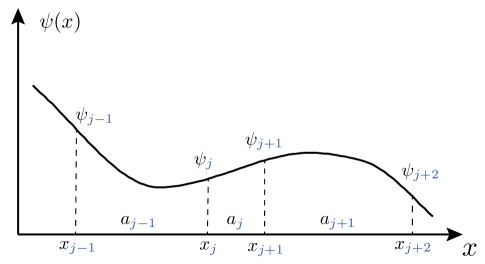
We discretize real space using a set of grid points $\{x_{j}\}$ (see Fig.(3)). The distance between two successive points is given by $a_{\color[rgb]{0,0,1}j}\!=\!x_{{\color[rgb]{0,0,1}j+1}}\!-\!x_{{\color[rgb]{0,0,1}j}}$. Now, a function $\psi(x)$ and its first and second derivatives $\psi^{\prime}(x)$ and $\psi^{\prime\prime}(x)$ are discretized as

$\displaystyle\psi_{{\color[rgb]{0,0,1}j}}$ $\displaystyle=\psi(x_{\color[rgb]{0,0,1}j}),$
$\displaystyle\psi^{\prime}_{{\color[rgb]{0,0,1}j+1/2}}$ $\displaystyle=\frac{\psi(x_{{\color[rgb]{0,0,1}j+1}})-\psi(x_{\color[rgb]{0,0,1}j})}{a_{\color[rgb]{0,0,1}j}},$
$\displaystyle\psi_{{\color[rgb]{0,0,1}j}}^{\prime\prime}$ $\displaystyle=\frac{\psi_{{\color[rgb]{0,0,1}j+1/2}}^{\prime}-\psi_{{\color[rgb]{0,0,1}j-1/2}}^{\prime}}{\frac{a_{{\color[rgb]{0,0,1}j}}+a_{{\color[rgb]{0,0,1}j-1}}}{2}}=2\frac{\frac{\psi_{{\color[rgb]{0,0,1}j+1}}-\psi_{{\color[rgb]{0,0,1}j}}}{a_{{\color[rgb]{0,0,1}j}}}-\frac{\psi_{{\color[rgb]{0,0,1}j}}-\psi_{{\color[rgb]{0,0,1}j-1}}}{a_{{\color[rgb]{0,0,1}j-1}}}}{a_{{\color[rgb]{0,0,1}j}}+a_{{\color[rgb]{0,0,1}j-1}}}$
$\displaystyle\simeq\frac{1}{a_{{\color[rgb]{0,0,1}j-1}}^{2}}\psi_{{\color[rgb]{0,0,1}j-1}}-\left(\frac{1}{a_{{\color[rgb]{0,0,1}j-1}}^{2}}+\frac{1}{a_{{\color[rgb]{0,0,1}j}}^{2}}\right)\psi_{{\color[rgb]{0,0,1}j}}+\frac{1}{a_{{\color[rgb]{0,0,1}j}}^{2}}\psi_{{\color[rgb]{0,0,1}j+1}},$ (E.1)

where we demanded that the spacing changes smoothly as a function of ${\color[rgb]{0,0,1}j}$, implying $(a_{{\color[rgb]{0,0,1}j}}+a_{{\color[rgb]{0,0,1}j-1}})a_{{\color[rgb]{0,0,1}j}}\!\simeq\!2a_{{\color[rgb]{0,0,1}j}}^{2}$ and $(a_{{\color[rgb]{0,0,1}j}}+a_{{\color[rgb]{0,0,1}j-1}})a_{{\color[rgb]{0,0,1}j-1}}\!\simeq\!2a_{{\color[rgb]{0,0,1}j-1}}^{2}$. Note that the first derivative is defined ‘in between’ grid points. Hence, the discretized version of the Hamiltonian $H(x)\!=\!-\frac{\hbar^{2}}{2m}\partial_{x}^{2}\!+\!V(x)$ at a point $x_{j}$ is given by

$\displaystyle H\psi_{{\color[rgb]{0,0,1}j}}=-\tau_{{\color[rgb]{0,0,1}j-1}}\psi_{{\color[rgb]{0,0,1}j-1}}-\tau_{j}\psi_{{\color[rgb]{0,0,1}j+1}}+E_{{\color[rgb]{0,0,1}j}}\psi_{{\color[rgb]{0,0,1}j}},$ (E.2)

with site-dependent hopping $\tau_{{\color[rgb]{0,0,1}j}}\!=\!1/(2ma_{{\color[rgb]{0,0,1}j}}^{2})$ (here and below we set $\hbar\!=\!1$) and the onsite-energy $E_{{\color[rgb]{0,0,1}j}}=\tau_{{\color[rgb]{0,0,1}j-1}}+\tau_{{\color[rgb]{0,0,1}j}}+V_{{\color[rgb]{0,0,1}j}}$.

References