Study of Anomaly Detection Based on Randomized Subspace Methods in IP Networks

Abstract

In this paper we propose novel randomized subspace methods to detect anomalies in Internet Protocol networks. Given a data matrix containing information about network traffic, the proposed approaches perform a normal-plus-anomalous matrix decomposition aided by random subspace techniques and subsequently detect traffic anomalies in the anomalous subspace using a statistical test. Experimental results demonstrate improvement over the traditional principal component analysis-based subspace methods in terms of robustness to noise and detection rate.

Keywords— anomaly detection, PCA subspace methods, orthonormal basis, $Q$-statistic.

1 Introduction

Network anomalies typically refer to abnormal behavior in the network traffic such as traffic volume, bandwidth and protocol use, which indicate a potential threat. Traffic anomalies may arise due to various causes ranging from network attacks such as denials-of-service (DoS) and network scans, to atypical circumstances such as flash-crowds and failures, which can have serious destructive effects on the performance and security of Internet Protocol (IP) networks [1], [2].

The seminal paper by Lakhina et al. [3] first employed Principal Component Analysis (PCA) [4] to detect network-wide traffic anomalies. Given a matrix of link traffic data ${\bf Y}$, the approach performs a normal-plus-anomalous matrix decomposition (i.e., ${\bf Y}=\hat{\bf Y}+\tilde{\bf Y}$) using (a specific number of) its principal components and seeks anomalies in the anomalous subspace $\tilde{\bf Y}$. The emergence of this approach inspired researchers to improve its performance and to evaluate its sensitivity for detecting anomalies [5], [6]. Ringberg et al. [5] point out that since PCA does not consider the temporal correlation of the data, the normal subspace is contaminated with anomalies. To address this issue, Brauckhoff et al. [6] propose to apply the Karhunen-Loeve (KL) expansion [7], which considers both the temporal and spatial correlations. Recently, inspired by the well-established compressed sensing (CS) theory [8], [9] and also by robust principal component analysis (RPCA) [10], [11], [12], several works have approached network-wide traffic anomaly detection using these methods (i.e., by solving a constrained optimization problem) [13], [14].

The PCA-based methods [3], [15], [6] focus on link traffic covariance matrix and accordingly compute its singular value decomposition (SVD), a computationally expensive factorization, to separate the subspaces. In this paper, we present two novel randomized subspace approaches to detect anomalies in network traffic. In contrast to the works in [3], [15], [6], the proposed approaches do not form the covariance matrix and consequently obviate the computation of the SVD for subspace separation. We validate the proposed approaches using synthetically generated data. Experimental results demonstrate that the proposed techniques can successfully diagnose network-wide anomalies with more effectiveness than PCA and robust PCA (RPCA).

The remainder of this paper is organized as follows. In Section 2 we introduce the signal model that represents IP traffic and formulate the problem we are interested in solving. We review the method of PCA for network anomaly detection in Section 3. In Section 4, we describe our proposed methods in detail. In Section 5, we present and discuss our experimental results and our conclusion remarks are given in Section 6.

2 Signal Model and Problem Formulation

In this section, we describe a signal model that represents the traffic in an IP network using linear algebra and state the problem of interest. Based on the structure of a network and the flow of data obtained by network tomography [16], we can model the link traffic as a function of the origin-destination (OD) flow traffic and the network-specific routing. Specifically, the relationship between the link traffic ${\bf Y}\in\mathbb{R}^{m\times t}$ and OD flow traffic ${\bf X}\in\mathbb{R}^{n\times t}$, for a network with $m$ links and $n$ OD flows may be written as:

$${\bf Y}={\bf R}{\bf X},$$ (1)

where $t$ is the number of snapshots and ${\bf R}\in\mathbb{R}^{m\times n}$ is a routing matrix. The entries of ${\bf R}$, i.e., ${\bf R}_{i,j}$, are assigned a value equal to one (${\bf R}_{i,j}=1$) if the OD flow $j$ traverses link $i$, and are assigned a value equal to zero otherwise.

The network traffic model that takes into account the anomalies and the measurement noise over the links can be expressed by

$${\bf Y}={\bf R}({\bf X}+{\bf A})+{\bf V},$$ (2)

where ${\bf R}\in\mathbb{R}^{m\times n}$ is a fixed routing matrix, ${\bf X}\in\mathbb{R}^{n\times t}$ is the clean traffic matrix, ${\bf A}\in\mathbb{R}^{n\times t}$ is the matrix with traffic anomalies and ${\bf V}\in\mathbb{R}^{m\times t}$ denotes the link measurement noise samples. The problem we are interested in this work is how detect anomalies by observing ${\bf Y}$.

3 Principal Component Analysis for Network Anomaly Detection

Given the link traffic ${\bf Y}$, in order to detect anomalies the work in [3] performs a normal-plus-anomalous matrix decomposition such that ${\bf Y}=\hat{\bf Y}+\tilde{\bf Y}$, where $\hat{\bf Y}$ is the modeled traffic and $\tilde{\bf Y}$ is the projection of ${\bf Y}$ onto the anomalous subspace $\tilde{\mathcal{S}}$, using a selected number of its principal components.

The modeled traffic represented by $\hat{\bf Y}$ is the projection of ${\bf Y}$ onto the normal subspace $\mathcal{S}$ and the residual traffic modeled by $\tilde{\bf Y}$ is the projection of ${\bf Y}$ onto the anomalous subspace $\tilde{\mathcal{S}}$. Specifically, the modeled traffic can be obtained by

$$\hat{\bf Y}={\bf P}{\bf P}^{T}{\bf Y}=\hat{\bf C}{\bf Y}$$ (3)

and

$$\tilde{\bf Y}=({\bf I}-{\bf P}{\bf P}^{T}){\bf Y}=\tilde{\bf C}{\bf Y},$$ (4)

where ${\bf P}=[{\bf w}_{1},{\bf w}_{2},...,{\bf w}_{r}]$ is formed by the first $r$ singular vectors of the covariance of the centered traffic data $\hat{\bf\Sigma}=\frac{1}{t-1}({\bf{Y-\mu}})({\bf{Y-\mu}})^{T}$ and $\hat{\bf\Sigma}={\bf W}{\bf\Lambda}{\bf W}^{T}$ is a singular value decomposition.

In order to detect abnormal changes in $\tilde{\bf Y}$, a statistic referred to as the $Q$-statistic [17] is applied by computing the squared prediction error (SPE) of the residual traffic:

$${\text{SPE}}={\|\tilde{\bf Y}\|_{2}^{2}}={\|\tilde{\bf C}{\bf Y}\|_{2}^{2}},$$ (5)

The network traffic is considered to be normal if

$${\text{SPE}}\leq Q_{\beta},$$ (6)

where $Q_{\beta}$ is a threshold for the SPE defined as:

$$Q_{\beta}=\theta_{1}\Big{[}\frac{c_{\beta}\sqrt{2\theta_{2}h_{0}^{2}}}{\theta_{1}}+1+\frac{\theta_{2}h_{0}(h_{0}-1)}{\theta_{1}^{2}}\Big{]}^{\frac{1}{h_{0}}},$$ (7)

where

$$h_{0}=1-\frac{2\theta_{1}\theta_{3}}{3\theta_{2}^{2}}$$ (8)

and

$$\theta_{i}=\sum_{j=k+1}^{m}\lambda_{j}^{i},\text{for}\mspace{6.0mu}i=1,2,3$$ (9)

with $\lambda_{j}$ denoting the $j$-th singular value of $\hat{\bf\Sigma}$ and $c_{\beta}$ is the $1-\beta$ percentile in a standard normal distribution.

The singular vectors of $\hat{\bf\Sigma}$ (or principal components of ${\bf Y}$) maximize the variance of the projected data. Thus, for instance, the $j$-the singular value of $\hat{\bf\Sigma}$ (or the variance captured by the $j$-the PC) can be expressed as $\lambda_{j}=\mathbb{V}{\text{ar}}\{({{\bf w}_{j}}^{T}{\bf Y})^{T}\}$. Note that, each row in ${\bf Y}$, $Y_{i}\in\mathbb{R}^{1\times t}$.

4 Proposed Subspace-Projected Basis for Anomaly detection

This section describes our proposed approaches termed Randomized Bases Anomaly Detection (RBAD) and Switched Subspace-Projected Bases for Anomaly Detection (SSPBAD). Similar to the works in [18] and [3], given the data traffic matrix ${\bf Y}$, RBAD and SSPBAD perform a normal-plus-anomalous matrix decomposition. However, instead of the principal components of ${\bf Y}$, they employ a matrix with a set of orthonormal bases ${\bf Q}\in\mathbb{R}^{m\times m}$ whose range approximates the range of ${\bf Y}$. Once ${\bf Q}$ is constructed, as will be explained in the next subsections, ${\bf Y}$ is represented as a linear superposition of normal and anomalous components (${\bf Y}=\hat{\bf Y}+\tilde{\bf Y}$) as given by

$$\hat{\bf Y}={\bf P}{\bf P}^{T}{\bf Y}=\hat{\bf C}{\bf Y}$$ (10)

and

$$\tilde{\bf Y}=({\bf I}-{\bf P}{\bf P}^{T}){\bf Y}=\tilde{\bf C}{\bf Y},$$ (11)

where the matrix ${\bf P}=[{\bf q}_{1},{\bf q}_{2},...,{\bf q}_{r}]$ contains the first $r$ columns of ${\bf Q}$. Accordingly, the variances captured by the orthonormal basis are computed as:

$${\bf\Lambda_{Q}}=\mathbb{V}{\text{ar}}\{({{\bf Q}^{T}{\bf Y})^{T}\}}$$ (12)

Then, the $Q$-statistic is applied to the anomalous component to diagnose anomalies. In contrast to [18] and [3], the proposed approaches do not require the estimation of the covariance matrix from the data and, as a result, the SVD is not required to be computed to separate subspaces. This also results in the reduction of the number of floating-point operations (flops) to detect anomalies in the traffic network.

4.1 Randomized Basis Anomaly Detection

To separate normal and anomalous subspaces as in (3), RBAD uses orthonormal bases whose range approximates the range of the traffic matrix ${\bf Y}$ (instead of the singular vectors of $\hat{\bf\Sigma}$ used in [18] and [3]). To compute the bases, the product ${\bf B}={\bf Y}{\bf\Phi}$ is first formed using a random matrix ${\bf\Phi}\in\mathbb{R}^{t\times m}$ and a $QR$ factorization is then performed on ${\bf B}$ (i.e., ${\bf Q}{\bf R}={\bf B}$) [19]. To improve the approximation accuracy the work in [19] multiplies ${\bf B}$ with ${\bf Y}$ and ${\bf Y}^{T}$ alternately. Once the bases are obtained, the variances captured by ${\bf Q}$ are calculated (i.e., ${\bf\Lambda_{Q}}=\mathbb{V}{\text{ar}}\{({{\bf Q}^{T}{\bf Y})^{T}\}}$) to detect abnormal behavior in anomalous components. Moreover, to apply $Q$-statistics the variances must be known [17], [20]. A pseudocode for RBAD is given in Table 1.

Table 1: Pseudocode for the proposed RBAD technique.

 

 

0:     traffic matrix $\ {\bf Y}\in\mathbb{R}^{m\times t},{\text{rank}}\mspace{6.0mu}r,{\text{an exponent}}\mspace{6.0mu}q$;

1:  Generate a random matrix $\bf\Phi$;

2:  Form ${\bf B}=({\bf Y}{\bf Y}^{T})^{q}{\bf Y\Phi}$;

3:  Perform a QR factorization to build an orthonormal basis: ${\bf B}={\bf Q}{\bf R}$;

4:  Compute the variances: ${\bf\Lambda_{Q}}=\mathbb{V}{\text{ar}}\{({{\bf Q}^{T}{\bf Y})^{T}\}}$;

5:  Separate the subspaces with rank $r$: ${\bf Y}=\hat{\bf Y}+\tilde{\bf Y}$;

6:  Apply $Q$-statistic to $\tilde{\bf Y}$: if SPE $>Q_{\beta}\rightarrow$ anomalies;

7:  return  anomalies in $\bf A$

 

 

4.2 Switched Subspace-Projected Basis for Anomaly Detection

The proposed SSPBAD technique, similar to RBAD, also constructs bases with orthonormal columns whose range approximates the range of ${\bf Y}$ which based on projects the traffic data ${\bf Y}$ onto two subspaces orthogonal to each other ( $\hat{\mathcal{S}}$ and $\tilde{\mathcal{S}}$). First, the product ${{\bf T}_{1}}={{\bf Y}^{T}}{{\bf T}_{2}}$ is formed using a random matrix ${{\bf T}_{2}}\in\mathbb{R}^{m\times m}$. Next, ${{\bf T}_{2}}$ is updated by ${{\bf T}_{1}}$ such that ${{\bf T}_{2}}={\bf Y}{{\bf T}_{1}}$. Afterwards, a $QR$ factorization is performed to construct the orthonormal bases for the range of ${{\bf T}_{2}}$. These orthonormal bases will serve as a surrogate to the bases of principal components used in [18] and [3] to separate normal and anomalous subspaces. Subsequently, the variances captured by ${\bf Q}$ are computed (i.e., ${\bf\Lambda_{Q}}=\mathbb{V}{\text{ar}}\{({{\bf Q}^{T}{\bf Y})^{T}\}}$) to detect traffic anomalies in the anomalous component using the $Q$-statistic.

A similar approach to constructing the orthonormal bases as in SSPBAD was proposed in [21] to approximate a rank-$r$ matrix, but they construct the bases for the range of ${{\bf T}_{1}}$. To increase robustness of the algorithm for detecting anomalies, we employ different matrices ${{\bf T}_{2}}$ as in [22], [23, 24, 25, 26, 27, 28, 29, 30, 31, 32, 33, 34, 35, 36]. The random matrices generated include:

• a matrix with i.i.d Gaussian entries i.e., $\mathcal{N}(0,1)$,

• a matrix whose entries are i.i.d. random variables drawn from a Bernoulli distribution with probability 0.5,

• a Markov matrix whose entries are all nonnegative and the entries of each column add up to 1,

• a matrix whose entries are independently drawn from $\{$-1, 1$\}$.

Thus, SSPBAD switches among different random matrices and chooses the best one in order to obtain the maximum number of anomalies. A pseudocode for SSPBAD is given in Table 2.

Table 2: Pseudocode for the proposed SSPBAD technique.

 

 

0:     traffic matrix $\ {\bf Y}\in\mathbb{R}^{m\times t},{\text{rank}}\mspace{6.0mu}r$;

1:  Generate $N$ random matrices ${{\bf T}_{2}}$;

2:  for $i=$ 1: $N$ do

3:     Form ${{\bf T}_{1}}$: ${{\bf T}_{1}}={{\bf Y}^{T}}{{\bf T}_{2}}$;

4:     Update ${{\bf T}_{2}}$: ${{\bf T}_{2}}={\bf Y}{{\bf T}_{1}}$;

5:     Perform a QR factorization to build orthonormal bases: ${\bf T}_{2}={\bf Q}{\bf R}$;

6:     Compute the variances: ${\bf\Lambda_{Q}}=\mathbb{V}{\text{ar}}\{({{\bf Q}^{T}{\bf Y})^{T}\}}$;

7:     Separate the subspaces with rank $r$: ${\bf Y}=\hat{\bf Y}+\tilde{\bf Y}$;

8:     Apply $Q$-statistic to $\tilde{\bf Y}$: if SPE $>Q_{\beta}\rightarrow$ anomalies;

9:  end for

10:  Choose the best random matrix with maximum number of anomalies;

11:  return  anomalies in $\bf A$

 

 

5 Experimental Results

To validate the proposed approaches, we conduct experiments on synthetically generated data and compare them with PCA and RPCA. The data matrix ${\bf Y}$ is generated according to the model in (2) with dimensions $m=120,n=240,t=640$. The low-rank matrix ${\bf X}$ is formed by a matrix multiplication ${\bf U}{\bf V}^{T}$, where ${\bf U}\in\mathbb{R}^{n\times r}$ and ${\bf V}\in\mathbb{R}^{t\times r}$ have Gaussian distributed entries $\mathcal{N}(0,1/n)$ and $\mathcal{N}(0,1/t)$, respectively and $r=0.2\times m$. The routing matrix ${\bf R}$ is generated by entries drawn from a Bernoulli distribution with probability $0.05$. The sparse matrix of anomalies has $s=0.001\times mt$ non-zero elements drawn randomly from the set $\{-1,1\}$ and the noise matrix ${\bf V}$ has independent and identically distributed (i.i.d) Gaussian entries with variance $\sigma^{2}$, i.e., $\mathcal{N}(0,\sigma^{2})$. We set the confidence limit $1-\beta=99.5\%$ for the value of the $Q$-statistic for all three approaches.

In Fig. 1, we compare the variances captured by the proposed approaches (orthonormal basis) with the PCA method (PCs) since they play a crucial role in the statistical test ($Q$-statistic) used to detect anomalies (cf. (8)). As can be seen, returned variances by RBAD and SSPBAD are very close to those returned by SVD.

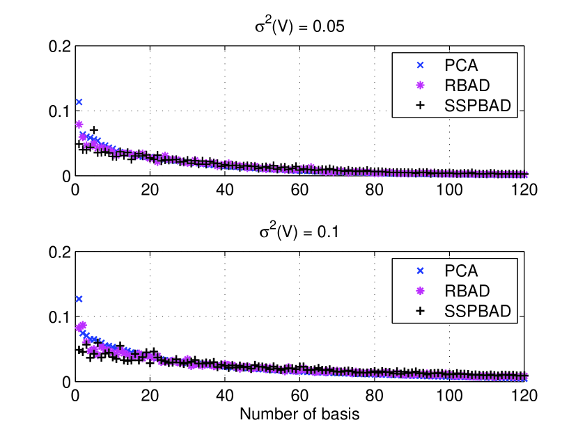
Figure 1: A comparison of variances for PCA, RBAD, SSPBAD.

Fig. 2 compares the detection rate against the number of bases for different approaches. As pointed out in [2] the detection rate combines false-alarm rate and detection probability into one measure and obviates the need for showing these two probabilities in one versus the other manner. As can be seen, the proposed RBAD and SSPBAD approaches outperform PCA when the measurement noise has a higher variance. Furthermore, RPCA [10],[11], [12] performs poorly. Since we consider measurement noises ${\bf V}$ in our data model (cf. 2), by increasing the rank, these noise samples contaminate the matrix of outliers returned by RPCA and as a result the abnormal patterns of the network (anomalies) cannot be recovered.

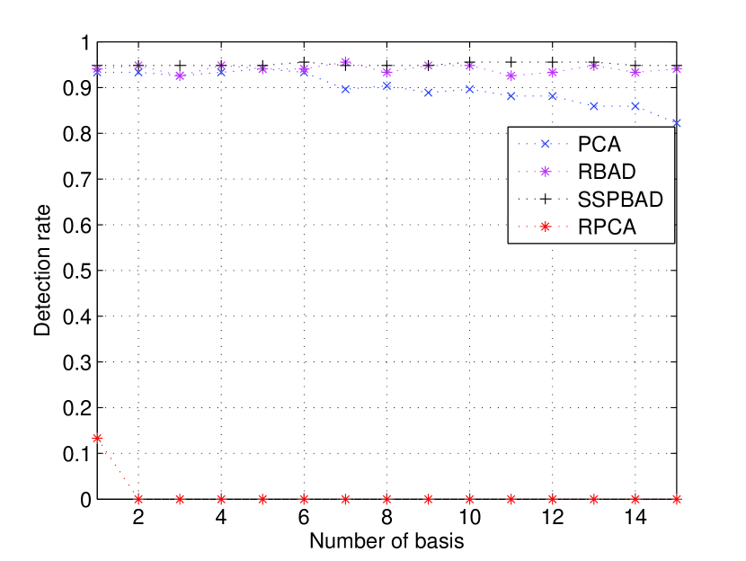
Figure 2: A comparison of detection rate for PCA, RBAD, SSPBAD and RPCA. Variance of the measurement noises $\sigma^{2}=0.1$

5.1 Computational Complexity

The traditional PCA method operates on the link traffic covariance ($\hat{\bf\Sigma}$) to separate the subspaces. In particular, PCA employs the SVD which requires $O(m^{3})$ floating-point operations (flops). RBAD and SSPBAD operate on the link traffic directly but employ the $QR$ factorization, which requires $O(m^{3})$ flops as well. Although the computational complexity of RBAD and SSPBAD is roughly the same as PCA in the context of anomaly detection, in certain applications where SVD cannot be efficiently used, an extension of the proposed approaches can be employed. For instance, they can be used to build a direct solver for contour integral equations with nonoscillatory kernels where the computational cost for a $QR$ factorization is considerably less prohibitive than that of SVD [37].

6 Conclusion

In this paper, we have proposed the RBAD and SSPBAD random subspace methods to detect traffic anomalies in IP networks. Both approaches form normal and anomalous randomized subspaces by orthonormal bases constructed for the range of the traffic data. A statistical test is then applied and detects anomalies in the traffic. Simulations show that RBAD and SSPBAD outperform PCA and RPCA. Future work will concentrate on mathematical analysis of RBAD and SSPBAD.

References

- [1] M. Thottan and C. Ji, “Anomaly detection in IP networks,” IEEE Transactions on Signal Processing, vol. 51, no. 8, pp. 2191 – 2204, aug 2003.
- [2] Y. Zhang, Z. Ge, A. Greenberg, and M. Roughan, “Network Anomography,” in Proceedings of the 5th ACM SIGCOMM conference on Internet Measurement (IMC ’05), oct 2005.
- [3] A. Lakhina, M. Crovella, and C. Diot, “Diagnosing Network-Wide Traffic Anomalies,” in proceedings of ACM SIGCOMM, aug 2004.
- [4] I. T. Jolliffe, “Principal Component Analysis,” 2nd ed, Springer, 2002.
- [5] H. Ringberg, A. Soule, J. Rexford, and C. Diot, “Sensitivity of PCA for traffic anomaly detection,” in Proceedings of the 2007 ACM SIGMETRICS international conference on Measurement and modeling of computer systems, jun 2007, pp. 109–120.
- [6] D. Brauckhoff, K. Salamatian, and M. Martin, “Applying PCA for Traffic Anomaly Detection: Problems and Solutions,” in Proceedings of INFOCOM 2009, apr 2009, pp. 2866 – 2870.
- [7] R. M. Gray and L. D. Davisson, “An Introduction to Statistical Signal Processing,” Cambridge University Press, 2005.
- [8] D. L. Donoho, “Compressed Sensing,” IEEE Transactions on Information Theory, vol. 52, no. 4, pp. 1289 – 1306, apr 2006.
- [9] E. J. Candès, J. Romberg, and T. Tao, “Exact Signal Reconstruction From Highly Incomplete Frequency Information,” IEEE Transactions on Information Theory, vol. 52, no. 2, pp. 489 – 509, feb 2006.
- [10] V. Chandrasekaran, S. Sanghavi, P. a. Parrilo, and A. S. Willsky, “Rank-Sparsity Incoherence for Matrix Decomposition,” SIAM Journal on Optimization, vol. 21, no. 2, pp. 572–596, 2009.
- [11] J. Wright, Y. Peng, Y. Ma, A. Ganesh, and S. Rao, “Robust Principal Component Analysis: Exact Recovery of Corrupted Low-Rank Matrices,” Advances in Neural Information Processing Systems (NIPS), pp. 2080–2088, 2009.
- [12] E. J. Candès, X. Li, Y. Ma, and J. Wright, “Robust principal component analysis?” Journal of the ACM, vol. 58, no. 3, pp. 1–37, may 2011.
- [13] M. Roughan, Y. Zhang, W. Willinger, and L. Qiu, “Spatio-Temporal Compressive Sensing and Internet Traffic Matrices (Extended Version),” IEEE/ACM Transactions on Networking, vol. 20, no. 3, pp. 662 – 676, jun 2012.
- [14] M. Mardani and G. B. Giannakis, “Estimating Traffic and Anomaly Maps via Network Tomography,” IEEE/ACM Transactions on Networking, vol. 24, no. 3, pp. 1533 – 1547, jun 2016.
- [15] L. Huang, X. Nguyen, M. Garofalakis, M. Jordan, A. D. Joseph, and N. Taft, “In-network pca and anomaly detection,” EECS Department, University of California, Berkeley, Tech. Rep. UCB/EECS-2007-10, Jan 2007. [Online]. Available: http://www.eecs.berkeley.edu/Pubs/TechRpts/2007/EECS-2007-10.html
- [16] Y. Vardi, “Network Tomography: Estimating Source-Destination Traffic Intensities from Link Data,” Journal of the American Statistical Association, no. 433, pp. 365–377, feb 1996.
- [17] J. E. Jackson and G. S. Mudholkar, “Control procedures for residuals associated with principal component analysis,” Technometrics, vol. 21, no. 3, pp. 341–349, aug 1979.
- [18] R. Dunia and S. J. Qin, “A Subspace Approach to Multidimensional Fault Identification and Reconstruction,” American Institute of Chemical Engineers (AIChE) Journal, vol. 44, no. 8, pp. 1813––1831, aug 1998.
- [19] N. Halko, P.-G. Martinsson, and J. A. Tropp, “Finding structure with randomness: Probabilistic algorithms for constructing approximate matrix decompositions,” SIAM Rev, vol. 53, no. 2, pp. 217–288, Jun 2011.
- [20] J. E. Jackson, “A User’s Guide to Principal Components,” New York: Wiley, 1991.
- [21] T. Zhou and D. Tao, “Godec: Randomized low-rank & sparse matrix decomposition in noisy case,” in ICML, 2011.
- [22] M. F. Kaloorazi and R. C. de Lamare, “Switched-Randomized Robust PCA for Background and Foreground Separation in Video Surveillance,” in IEEE SAM 2016, jul 2016.
- [23] R. C. de Lamare and R. Sampaio-Neto, “Adaptive Reduced-Rank Processing Based on Joint and Iterative Interpolation, Decimation, and Filtering,” IEEE Transactions on Signal Processing, vol. 57, no. 7, pp. 2503–2514, jul 2009.
- [24] R. Fa and R. C. De Lamare, “Multi-branch successive interference cancellation for mimo spatial multiplexing systems: design, analysis and adaptive implementation,” IET communications, vol. 5, no. 4, pp. 484–494, 2011.
- [25] R. C. de Lamare and R. Sampaio-Neto, “Minimum mean-squared error iterative successive parallel arbitrated decision feedback detectors for ds-cdma systems,” IEEE Transactions on Communications, vol. 56, no. 5, pp. 778–789, 2008.
- [26] R. C. De Lamare and R. Sampaio-Neto, “Adaptive reduced-rank mmse filtering with interpolated fir filters and adaptive interpolators,” IEEE Signal Processing Letters, vol. 12, no. 3, pp. 177–180, 2005.
- [27] R. Fa, R. C. de Lamare, and L. Wang, “Reduced-rank stap schemes for airborne radar based on switched joint interpolation, decimation and filtering algorithm,” IEEE Transactions on Signal Processing, vol. 58, no. 8, pp. 4182–4194, 2010.
- [28] Y. Zhaocheng, R. De Lamare, and L. Xiang, “L1 regularized stap algorithm with a generalized sidelobe canceler architecture for airborne radar,” IEEE Transactions on Signal Processing, vol. 60, no. 2, pp. 674–686, 2012.
- [29] R. de Lamare, “Adaptive and iterative multi-branch mmse decision feedback detection algorithms for multi-antenna systems,” IEEE Transactions on Wireless Communications, vol. 12, no. 10, pp. 5294–5308, 2013.
- [30] T. Peng, R. de Lamare, and A. Schmeink, “Adaptive distributed space-time coding based on adjustable code matrices for cooperative mimo relaying systems,” IEEE Transactions on Communications, vol. 61, no. 7, pp. 2692–2703, 2013.
- [31] S. Li, R. C. de Lamare, and R. Fa, “Reduced-rank linear interference suppression for ds-uwb systems based on switched approximations of adaptive basis functions,” IEEE Transactions on Vehicular Technology, vol. 60, no. 2, pp. 485–497, 2011.
- [32] S. Xu, R. C. de Lamare, and H. V. Poor, “Distributed compressed estimation based on compressive sensing,” IEEE Signal Processing Letters, vol. 22, no. 9, pp. 1311–1315, 2015.
- [33] ——, “Adaptive link selection algorithms for distributed estimation,” EURASIP Journal on Advances in Signal Processing, vol. 2015, no. 1, p. 86, 2015.
- [34] Y. Cai, R. C. de Lamare, L.-L. Yang, and M. Zhao, “Robust mmse precoding based on switched relaying and side information for multiuser mimo relay systems,” IEEE Transactions on Vehicular Technology, vol. 64, no. 12, pp. 5677–5687, 2015.
- [35] F. G. A. Neto, R. C. De Lamare, V. H. Nascimento, and Y. V. Zakharov, “Adaptive reweighting homotopy algorithms applied to beamforming,” IEEE Transactions on Aerospace and Electronic Systems, vol. 51, no. 3, pp. 1902–1915, 2015.
- [36] T. Peng and R. C. de Lamare, “Adaptive buffer-aided distributed space-time coding for cooperative wireless networks,” IEEE Transactions on Communications, vol. 64, no. 5, pp. 1888–1900, 2016.
- [37] H. Cheng, Z. Gimbutas, P. G. Martinsson, and V. Rokhlin, “On the compression of low rank matrices,” SIAM Journal on Scientific Computing (SISC), vol. 26, no. 4, p. 1389 – 1404, 2005.