Gait transitions in a phase oscillator model
of an insect central pattern generator

Abstract

Legged locomotion involves various gaits. It has been observed that fast running insects (cockroaches) employ a tripod gait with three legs lifted off the ground simultaneously in swing, while slow walking insects (stick insects) use a tetrapod gait with two legs lifted off the ground simultaneously. Fruit flies use both gaits and exhibit a transition from tetrapod to tripod at intermediate speeds. Here we study the effect of stepping frequency on gait transition in an ion-channel bursting neuron model in which each cell represents a hemi-segmental thoracic circuit of the central pattern generator. Employing phase reduction, we collapse the network of bursting neurons represented by 24 ordinary differential equations to 6 coupled nonlinear phase oscillators, each corresponding to a sub-network of neurons controlling one leg. Assuming that the left and right legs maintain constant phase differences (contralateral symmetry), we reduce from 6 equations to 3, allowing analysis of a dynamical system with 2 phase differences defined on a torus. We show that bifurcations occur from multiple stable tetrapod gaits to a unique stable tripod gait as speed increases. Finally, we consider gait transitions in two sets of data fitted to freely walking fruit flies.

Key words. bifurcation, bursting neurons, coupling functions, insect gaits, phase reduction, phase response curves, stability

AMS subject classifications. 34C16, 34C60, 37G10, 92B20, 92C20

1 Introduction: idealized insect gaits

Legged locomotion involves alternating stance and swing phases in which legs respectively provide thrust to move the body and are then raised and repositioned for the next stance phase. Insects, having six legs, are capable of complex walking gaits in which various combinations of legs can be simultaneously in stance and swing. However, when walking on level ground, their locomotive behavior can be characterized by the following kinematic rules, [1, 2].

1. A wave of protractions (swing) runs from posterior to anterior legs.

2. Contralateral legs of the same segment alternate approximately in anti-phase.

   In addition, in [1], Wilson assumed that:

3. Swing duration remains approximately constant as speed increases.

4. Stance (retraction) duration decreases as speed increases.

Rules 3 and 4 have been documented in fruit flies by Mendes et. al. [3].

In the slow metachronal gait, the hind, middle and front legs on one side swing in succession followed by those on the other side; at most one leg is in swing at any time. As speed increases, in view of rules 3 and 4, the swing phases of contralateral pairs of legs begin to overlap, so that two legs swing while four legs are in stance in a tetrapod gait, as observed for fruit flies in [3]. At the highest speeds the hind and front legs on one side swing together with the contralateral middle leg while their contralateral partners provide support in an alternating tripod gait which is typical for insects at high speeds.

Motivated by observations and data from fruit flies, which use both tetrapod and tripod gaits, and from cockroaches, which use tripod gaits [4], and stick insects, which use tetrapod gaits [5], our goal is to understand the transition between these gaits and their stability properties, analytically. Our dynamical analysis provides a mechanism that supplements the kinematic description given above. This will allow us to distinguish tetrapod, tripod, and transition gaits precisely and ultimately to obtain rigorous results characterizing their existence and stability. For gait transitions in vertebrate animals, see e.g. [6, 7].

In [4], a $6$-oscillator model, first proposed in [8], was used to fit data from freely running cockroaches that use tripod gaits over much of their speed range [9]. Here, in addition to the tripod gait, we consider tetrapod gaits and study the transitions among them and tripod gaits. We derive a $6$-oscillator model from a network of 6 bursting neurons with inhibitory nearest neighbor coupling. After showing numerically that it can produce multiple tetrapod gaits as well as a tripod gait, we appeal to the methods of phase reduction and bifurcation theory to study gait transitions. Our coupling assumption is supported by studies of freely running cockroaches in [4], in which various architectures were compared and inhibitory nearest neighbor coupling provided the best fits to data according to Akaike and Bayesian Information Criteria (AIC and BIC). The inhibitory assumption is motivated by the fact that neighboring oscillators’ solutions are out of phase [10].

Phase reduction is also used by Yeldesbay et. al. in [11, 12] to model stick insect locomotion and display gait transitions. Their reduced model contains 3 ipsilateral legs and has a cyclical coupling architecture, with a connection from hind to front segments. Here we show that the nearest neighbor architecture also produces such gait transitions.

Our main contributions are as follows. First, we confirm that speed changes in the bursting neuron model can be achieved by parameter variations (cf. [8, 13]) and we numerically illustrate that increasing speed leads to transition from tetrapod to tripod gaits. We then reduce the bursting neuron model from 24 ODEs to 2 phase difference equations and characterize coupling functions that produce these gait transitions. We illustrate them via analysis and simulations of the 24 ODE model and the phase difference equations, using parameters derived from fruit fly data, thereby showing biological feasibility of the mechanisms.

This paper is organized as follows. In Section 2, we review the ion-channel model for bursting neurons which was developed in [8, 13], study the influence of the parameters on speed and demonstrate gait transitions numerically. In Section 3, we describe the derivation of reduced phase equations, and define tetrapod, tripod and transition gaits. At any fixed speed, we assume constant phase differences between left- and right-hand oscillators, so that an ipsilateral network of 3 oscillators determines the dynamics of all 6 legs. We further reduce to a pair of phase-difference equations defined on a 2-dimensional torus. In Section 4 we prove the existence of tetrapod, tripod and transition gaits under specific conditions on the intersegmental coupling strengths, and establish their stability types.

In Section 5 we apply the results of Section 4 to the bursting neuron model. We show that the form of the coupling functions, which depend upon speed, imply the existence of transition solutions connecting tetrapod gaits to the tripod gait. In Section 6 we characterize a class of explicit coupling functions that exhibit transitions from tetrapod gaits to the tripod gait. As an example, we analyze phase-difference equations, using coupling functions approximated by Fourier series and derive bifurcation diagrams via branch-following methods. In Section 7 we describe gait transitions in a phase model with coupling strengths estimated by fitting data from freely running fruit flies, and show that such transitions occur even when coupling strengths are far from the special cases studied in Sections 4 and 5. We conclude in Section 8.

2 Bursting neuron model

In this section we define the bursting neuron model, describe its behavior, and illustrate the gait transitions in a system of 24 ODEs representing 6 coupled bursting neurons.

2.1 A single neuron

CPGs in insects are networks of neurons in the thoracic and other ganglia that produce rhythmic motor patterns such as walking, swimming, and flying. CPGs for rhythmic movements are reviewed in e.g. [14, 15]. In this work, we employ a bursting neuron model which was developed in [13] to model the local neural network driving each leg. This system includes a fast nonlinear current, e.g., $I_{Ca}$, a slower potassium current $I_{K}$, an additional very slow current $I_{KS}$, and a linear leakage current $I_{L}$. The following system of ordinary differential equations (ODEs) describes the bursting neuron model and its synaptic output $s(t)$.

$$C\dot{v} =-\left\{I_{Ca}(v)+I_{K}(v,m)+I_{KS}(v,{w})+I_{L}(v)\right\}+I_{ext},$$ (1a)

$$\dot{m} =\displaystyle\frac{\epsilon}{\tau_{m}(v)}[m_{\infty}(v)-m],$$ (1b)

$$\dot{{w}} =\displaystyle\frac{\delta}{\tau_{{w}}(v)}[{w}_{\infty}(v)-{w}],$$ (1c)

$$\dot{s} =\displaystyle\frac{1}{\tau_{s}}[s_{\infty}(v)(1-s)-s],$$ (1d)

where the ionic currents are of the following forms

$$I_{Ca}(v)\;=\;\bar{g}_{Ca}n_{\infty}(v)(v-E_{Ca}),\qquad I_{K}(v,m)\;=\;\bar{g}_{K}\;m\;(v-E_{K}),$$ (2)

$$I_{KS}(v,{w})\;=\;\bar{g}_{KS}{w}\;(v-E_{KS}),\qquad I_{L}(v)\;\;=\;\;\bar{g}_{L}(v-E_{L}).$$

The steady state gating variables associated with ion channels and their time scales take the forms

$$m_{\infty}(v)\;=\;\frac{1}{1+e^{-2k_{K}(v-v_{K})}}\;,\qquad\qquad{w}_{\infty}(v)\;=\;\frac{1}{1+e^{-2k_{KS}(v-v_{KS})}}\;,$$ (3)

$$n_{\infty}(v)\;=\;\frac{1}{1+e^{-2k_{Ca}(v-v_{Ca})}}\;,\qquad\qquad s_{\infty}(v)\;=\;\frac{a}{1+e^{-2k_{s}(v-E^{pre}_{s})}}\;,$$

and

$$\tau_{m}(v)=\mbox{sech}\,(k_{K}(v-v_{K})),\quad\tau_{{w}}(v)=\mbox{sech}\,(k_{KS}(v-v_{KS})).$$ (4)

Here the variable $s$ represents neurotransmitter released at the synapse and the constant parameter $\tau_{s}$ specifies the synaptic time scale. The constant parameters are generally fixed as specified in Table 1. Most of the parameter values are taken from [13], but some of our notations are different.

	$\delta$	$I_{ext}$	$\bar{g}_{Ca}$	$\bar{g}_{K}$	$\bar{g}_{KS}$	$\bar{g}_{L}$	$\bar{g}_{syn}$	$E_{Ca}$	$E_{K}$	$E_{KS}$	$E_{L}$	$E^{post}_{s}$
$\delta$ control	varies	35.6	4.4	9.0	0.19	2.0	0.01	120	-80	-80	-60	-70
$I_{ext}$ control	0.027	varies	4.4	9.0	0.5	2.0	0.01	120	-80	-80	-60	-70

	$k_{Ca}$	$k_{K}$	$k_{KS}$	$k_{s}$	$v_{Ca}$	$v_{K}$	$v_{KS}$	$E^{pre}_{s}$	a	$C$	$\epsilon$	$\tau_{s}$
$\delta$ control	0.056	0.1	0.8	0.11	-1.2	2	-27	2	55.56	1.2	4.9	5.56
$I_{ext}$ control	0.056	0.1	0.8	0.11	-1.2	2	-26	2	444.48	1.2	5.0	5.56

Table 1: The constant parameters in the bursting neuron model, as $\delta$ (first row) and $I_{ext}$ (second row) vary.

Figure 1 (first row) shows the solution of Equation (1) for the parameters specified in the first row of Table 1, and for $\delta=0.02$. Figure 1 (second row) shows the solution of Equation (1) for the parameters specified in the second row of Table 1, and for $I_{ext}=36.5$. We solved the equation using a fourth order explicit Runge-Kutta method in a custom-written code, with fixed time step, $0.001$ ms and ran the simulation for 1000 ms with initial conditions:

$$v(0)=-70,\;m(0)=-10,\;{w}(0)=-4,\;s(0)=2.$$

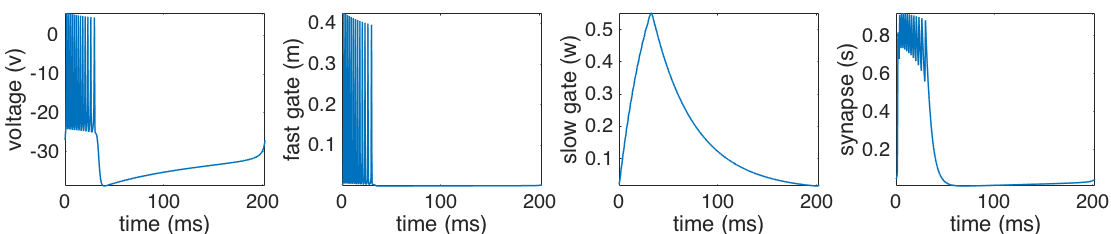
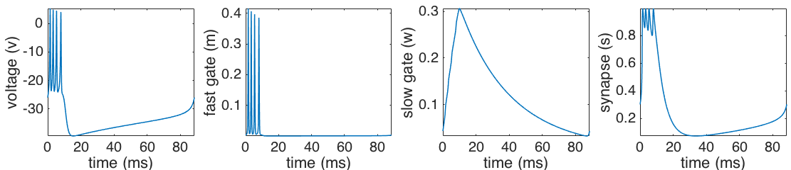
Figure 1: First row: A solution of Equation (1) for the parameters in the first row of Table 1, and for $\delta=0.02$. Second row: A solution of Equation (1) for the parameters in the second row of Table 1, and for $I_{ext}=36.5$. Each case is shown for one period of the bursting process.

The periodic orbit in $(v,m,{w})$ space contains a sequence of spikes (a burst) followed by a quiescent phase, which correspond respectively to the swing and stance phases of one leg. The burst from the CPG inhibits depressor motoneurons, allowing the swing leg to lift from the ground [8, 10] (see also [16, 17]). We denote the period of the periodic orbit by $T$, i.e., it takes $T$ time units (ms here) for an insect to complete the cycle of each leg. The number of steps completed by one leg per unit of time is the stepping frequency and is equal to $\omega=2\pi/T$. The period of the limit cycles shown in Figure 1 are approximately 202 ms and 88.57 ms, and their frequencies are approximately 4.95 Hz and 11.29 Hz, respectively. The swing phase ($SW$) is the duration of one burst and represents the time when the leg is off the ground, and the stance phase ($ST$) is the duration of the quiescence in each periodic orbit and represents the time when the leg is on the ground. Hence, $SW+ST=T$. The swing duty cycle, denoted by $DC$, is equal to $SW/T$. Note that an insect decreases its speed primarily by decreasing its stance phase duration (see the data in [3], and the rules from [1], given in the introduction).

In what follows, we show the effect of two parameters in the bursting neuron model, $\delta$ and $I_{ext}$, on period, swing, stance and duty cycle. We will see that these parameters have a major effect on speed; i.e., when either $\delta$ and $I_{ext}$ increase, the period of the periodic orbit decreases, primarily by decreasing stance phase duration, and so the insect’s speed increases. We consider the effects of each parameter separately but in parallel. As we study the effect of $\delta$ (resp. $I_{ext}$), we fix all other parameters as in the first (resp. second) row of Table 1. We let $\delta$ vary in the range ${\color[rgb]{0,0,0}{[\delta_{1},\delta_{2}]}}=[0.0097,0.04]$ and $I_{ext}$ vary in the range ${\color[rgb]{0,0,0}{[I_{1},I_{2}]}}=[35.65,37.7]$.

2.1.1 Effect of the slowest time scale $\delta$ and external input $I_{ext}$ on stepping frequency

Figure 2 shows the frequency, duty cycle, stance, and swing as functions of $\delta$. We computed these quantities by numerically solving the bursting neuron model (1) for a fixed set of parameters (first row of Table 1) as $\delta$ varies. As the figure depicts, as $\delta$ increases from $0.0097$ to $0.04$, stepping frequency increases from approximately $2.66$ Hz to $8.59$ Hz, i.e., the speed of the animal increases. Also, note that the stance and swing phase durations decrease, while the duty cycle remains approximately constant.

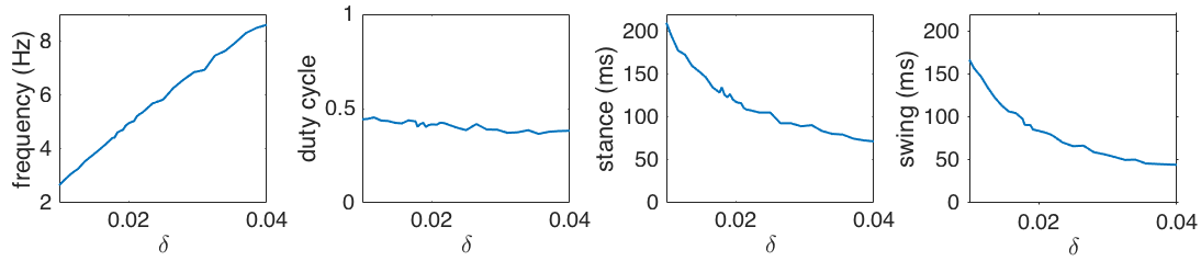
Figure 2: The effect of $\delta$ on frequency, duty cycle, stance, and swing in a single uncoupled bursting neuron model. See the first row of Table 1 for parameters.

We repeat the scenario with fixed parameters in the second row of Table 1 and varying $I_{ext}$. Figure 3 shows frequency, duty cycle, stance, and swing as functions of $I_{ext}$. As $I_{ext}$ increases from $35.65$ to $37.7$, stepping frequency increases from approximately $6.9$ Hz to $14.9$ Hz. Now, the duty cycle increases slightly, in contrast to Figure 2, while the swing duration remains approximately constant. This is closer to the rules given in Section 1.

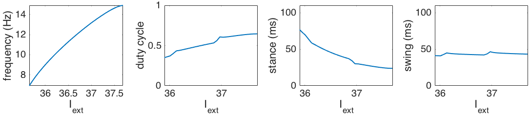
Figure 3: The effect of $I_{ext}$ on frequency, duty cycle, stance, and swing in a single uncoupled bursting neuron model. See the second rows of Table 1 for parameters.

For the rest of the paper, we use the symbol ${\xi}$ to denote the speed parameter $\delta$ or $I_{ext}$. We note that it is more realistic to use $I_{ext}$ as speed parameter, for the following three reasons.

1. Input currents provide a more biologically relevant control mechanism, [18].

2. Swing duration remains approximately constant, as proposed in rule 3 of Section 1, while $\delta$ affects burst duration [13].

3. The frequency range obtained is closer to that seen in fruit fly [3] and cockroach data [4].

Remark 1.

We have observed that $\bar{g}_{KS}$ has a similar influence on stepping frequency as $\delta$ and $I_{ext}$, but we will not study the effects of this parameter on gait transition in this paper.

2.2 Weakly interconnected neurons

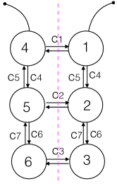
Figure 4: Network of CPGs

We now consider a network of six mutually inhibiting units, representing the hemi-segmental CPG networks contained in the insect’s thorax, as shown in Figure 4. We assume that inhibitory coupling is achieved via synapses that produce negative postsynaptic currents. The synapse variable $s$ enters the postsynaptic cell in Equation (1a) as an additional term, $I_{syn}$,

$$C\dot{v}_{i} =-\left\{I_{Ca}+I_{K}+I_{KS}+I_{L}\right\}+I_{ext}+I_{syn}\;,$$ (5)

where

$$I_{syn}=\sum_{j\in\mathcal{N}_{i}}I_{syn}(v_{i},s_{j})=\sum_{j\in\mathcal{N}_{i}}-\bar{c}_{ji}\bar{g}_{syn}s_{j}\left(v_{i}-E_{s}^{post}\right),$$ (6)

$\bar{g}_{syn}$ denotes the synaptic strength, and $\mathcal{N}_{i}$ denotes the set of the nodes adjacent to node $i$. The multiplicative factor $\bar{c}_{ji}$ accounts for the fact that multiple bursting neurons are interconnected in the real animals, and $-\bar{c}_{ji}\bar{g}_{syn}$ represents an overall coupling strength between hemi-segments. Following [4] we assume contralateral symmetry and include only nearest neighbor coupling, so that there are three contralateral coupling strengths ${c}_{1},{c}_{2},{c}_{3}$ and four ipsilateral coupling strengths ${c}_{4},{c}_{5},{c}_{6},$ and ${c}_{7}$; see Figure 4. For example, $\bar{c}_{21}={c}_{5}$, $\bar{c}_{41}={c}_{1},$ etc. Furthermore, we assume that all connections are inhibitory, i.e., $-{c}_{i}\bar{g}_{syn}<0$, therefore, all the ${c}_{i}$’s are positive.

A system of $24$ equations describes the dynamics of the $6$ coupled cells in the network as shown in Figure 4. We assume that each cell which is governed by Equation (1), represents one leg of the insect. Cells $1,2$, and $3$ represent right front, middle, and hind legs, and cells $4,5$, and $6$ represent left front, middle, and hind legs, respectively. For example, assuming that each cell is described by $(v_{i},m_{i},{w}_{i},s_{i})^{T}$, $i=1,\ldots,6$, the synapses from presynaptic cells $2$ and $4$, denoted by $s_{2}$ and $s_{4}$, respectively, enter the postsynaptic cell $1$. The following system of $4$ ODEs describe the dynamics of cell $1$ when connected to cells $2$ and $4$:

$$C\dot{v}_{1} =-\left\{I_{Ca}(v_{1})+I_{K}(v_{1},m_{1})+I_{KS}(v_{1},{w}_{1})+I_{L}(v_{1})\right\}+I_{ext}$$ (7)

$$\quad-{c}_{1}\bar{g}_{syn}s_{4}(v_{1}-E_{s}^{post})-{c}_{5}\bar{g}_{syn}s_{2}(v_{1}-E_{s}^{post}),$$

$$\dot{m}_{1} =\frac{\epsilon}{\tau_{m}(v_{1})}[m_{\infty}(v_{1})-m_{1}],$$

$$\dot{{w}}_{1} =\frac{\delta}{\tau_{{w}}(v_{1})}[{w}_{\infty}(v_{1})-{w}_{1}],$$

$$\dot{s}_{1} =\frac{1}{\tau_{s}}[s_{\infty}(v_{1})(1-s_{1})-s_{1}],$$

where ${c}_{1}$ and ${c}_{5}$ are the coupling strengths from cell $4$ and cell $2$ to cell $1$, respectively. Note that we assume contralateral symmetry, so the coupling strength from cell $1$ to cell $4$ is equal to the coupling strength from cell $4$ to cell $1$, etc. Five sets, each of analogous ODEs, describe the dynamics of the other five legs. Moreover, unlike the front and hind legs, the middle leg cells are connected to three neighbors; see Figure 4. Thus, the full model is described by 24 ODEs.

2.3 Tetrapod and tripod gaits

In this section, we show numerically the gait transition from tetrapod to tripod as the speed parameter ${\xi}$ increases. An insect is said to move in a tetrapod gait if at each step two legs swing in synchrony while the remaining four are in stance. The following four patterns are possible.

1. Forward right tetrapod: $(R2,L3),(R1,L2),(R3,L1)$.

2. Forward left tetrapod: $(R2,L1),(R1,L3),(R3,L2)$.

3. Backward right tetrapod: $(R2,L3),(R3,L1),(R1,L2)$.

4. Backward left tetrapod: $(R2,L1),(R3,L2),(R1,L3)$.

Here $R1,R2,R3$ denote the right front, middle and hind legs, and $L1,L2,L3$ denote the left front, middle and hind legs, respectively. The legs in each pair swing simultaneously, and touchdown of the legs in each pair coincides with lift off of the next pair. For example, in $(R1,L3)$, the right front leg and left hind legs are in synchrony, etc. Figure 5 (left) shows cartoons of an insect executing one cycle of the forward and backward tetrapod gaits, in which each leg completes one swing and one stance phase.

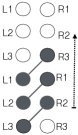
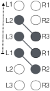
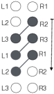
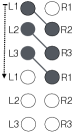
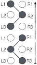
Figure 5: (Left to right) one cycle of forward right, forward left, backward right, backward left tetrapod gaits, and a tripod gait are shown. The diagonal lines connect legs that swing together; arrows indicate forward (resp. backward) waves.

In forward gaits, a forward wave of swing phases from hind to front legs causes a movement, while in backward gaits, the swing phases pass from front to hind legs. In right gaits, the right legs lead while in left gaits the left legs lead. We will exhibit a gait transition from forward right tetrapod to tripod as $I_{ext}$ varies, and a gait transition from forward left tetrapod to tripod as $\delta$ varies. Backward gaits have not been observed in forward walking; however, see Figure 29 and the corresponding discussion in the text.

An insect is said to move in a tripod gait (also called alternating tripod), when the following triplets of legs swing simultaneously, and touchdown of each triplet coincides with lift off of the other.

$$(R1,L2,R3),(L1,R2,L3).$$

Figure 5 (right) shows a cartoon of an insect executing one cycle of the tripod gait, in which each leg completes one swing and one stance phase.

Figure 6 depicts a gait transition from a forward right tetrapod to a tripod in the bursting neuron model as $I_{ext}$ increases (first column) and from a forward left tetrapod to a tripod as $\delta$ increases (second column), and for a fixed set of parameters, initial conditions, and coupling strengths ${c}_{i}$ as given below. Figure 7 shows the corresponding voltages. Coupling strengths ${c}_{i}$ are fixed at the following values for the simulations shown in Figures 6 and 7:

$${c}_{1}={c}_{2}={c}_{3}={c}_{4}=1,\;{c}_{5}={c}_{6}=3,\;{c}_{7}=2.$$ (8)

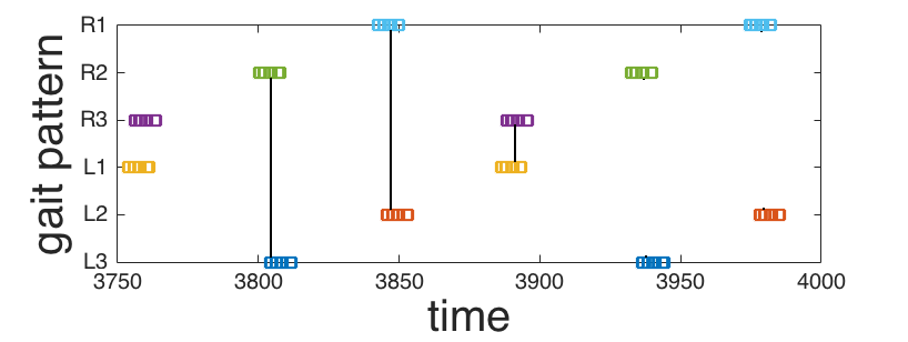
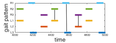
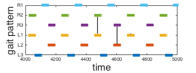
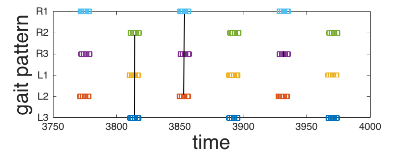
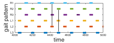
Figure 6: Interconnected bursting neuron model: gait transitions from forward right tetrapod to tripod as $I_{ext}$ increases, $I_{ext}=35.9,36.2,37.0$ (left column, top to bottom), and from forward left tetrapod to tripod as $\delta$ increases, $\delta=0.01,0.019,0.03$ (right column, top to bottom). Width of horizontal bars indicate swing durations. Note the transitional gaits with partial overlap of swing durations in the middle row.

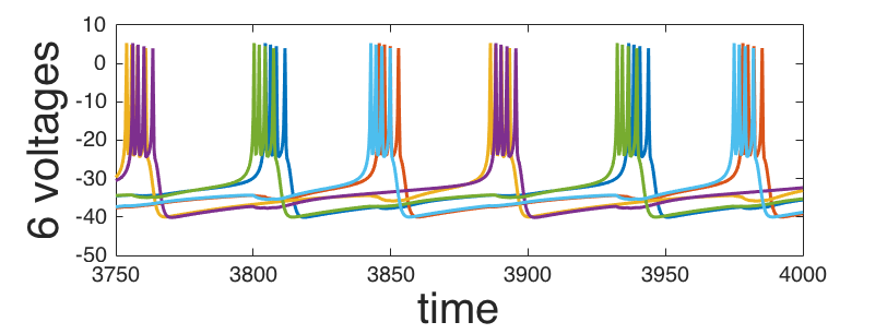
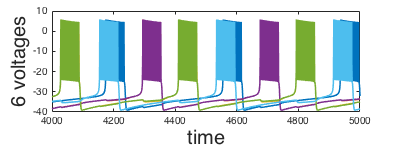
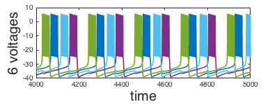
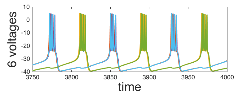
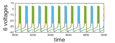
Figure 7: The corresponding voltages for the gaits presented in Figure 6. Color code matches that for legs in Figure 6. Note that some traces are hidden due to in-phase bursts.

In the simulations shown in first column of Figure 6 (as $I_{ext}$ varies), the 24 initial conditions for the 24 ODEs are equal to

$$v_{1}(0)=-31.93,\;v_{2}(0)=-38.55,\;v_{3}(0)=-23.83,\;v_{4}(0)=-24.12,\;v_{5}(0)=-31.93,\;v_{6}(0)=-38.55,$$ (9)

and for $i=1,\cdots,6$, $m_{i}$, ${w}_{i}$, and $s_{i}$ take their steady state values as in Equation (11). We computed the solutions up to time $t=4000$ ms but only show the time window $[3750,4000],$ after transients have died out. In the simulations shown in second column of Figure 6 (as $\delta$ varies), the 24 initial conditions for the 24 ODEs are equal to

$$v_{1}(0)=-10,\;v_{2}(0)=-40,\;v_{3}(0)=-30,\;v_{4}(0)=-40,\;v_{5}(0)=5,\;v_{6}(0)=20,$$ (10)

and for $i=1,\cdots,6$, $m_{i}$, ${w}_{i}$, and $s_{i}$ take their steady state values:

$$m_{i}(0)=m_{\infty}(v_{i}(0)),\;{w}_{i}(0)={w}_{\infty}(v_{i}(0)),\;s_{i}(0)=\frac{s_{\infty}(v_{i}(0))}{s_{\infty}(v_{i}(0))+1}.$$ (11)

We computed solutions up to time $t=5000$ ms but only show the time window $[4000,5000],$ after transients have died out.

Our goal is to show that, for the fixed set of parameters in Table 1, and appropriate coupling strengths ${c}_{i}$, as the speed parameter ${\xi}$, $I_{ext}$ or $\delta$, increases, a gait transition from (forward) tetrapod to tripod gait occurs. We will provide appropriate conditions on the ${c}_{i}$’s in Section 4. To reach our goal we first need to define the tetrapod and tripod gaits mathematically. To this end, in the following section, we reduce the interconnected bursting neuron model to $6$ interconnected phase oscillators, each describing one leg’s cyclical movement.

3 A phase oscillator model

In this section, we apply the theory of weakly coupled oscillators (see Section 9) to the coupled bursting neuron models to reduce the 24 ODEs to 6 phase oscillator equations. For a comprehensive review of oscillatory dynamics in neuroscience with many references see [19].

3.1 Phase equations for a pair of weakly coupled oscillators

Let the ODE

$$\dot{X}=f(X),\qquad X\in{\mathbb{R}}^{n},$$ (12)

describe the dynamics of a single neuron. In our model, $X=(v,m,{w},s)^{T}$ and $f(X)$ is as the right hand side of Equations (1). Assume that Equation (12) has an attracting hyperbolic limit cycle $\Gamma=\Gamma(t)$, with period $T$ and frequency ${\omega}=2\pi/T$.

Now consider the system of weakly coupled identical neurons

$$\dot{X}_{1}=f(X_{1})+\epsilon g(X_{1},X_{2}),$$ (13)

$$\dot{X}_{2}=f(X_{2})+\epsilon g(X_{2},X_{1}),$$

where $0<\epsilon\ll 1$ is the coupling strength and $g$ is the coupling function. The phase of a neuron, denoted by $\phi$, is the time that has elapsed as its state moves around $\Gamma$, starting from an arbitrary reference point in the cycle. For each neuron, the phase equation is:

$$\frac{d\phi_{i}}{dt}(t)=\omega+\epsilon H(\phi_{j}(t)-\phi_{i}(t)),$$ (14)

where

$$H=H(\theta)=\frac{1}{T}\int_{0}^{T}Z(\Gamma(\tilde{t}))\cdot g(\Gamma(\tilde{t}),\Gamma(\tilde{t}+\theta))\;d\tilde{t},$$

is the coupling function: the convolution of the synaptic current input to the neuron via coupling $g$ and the neuron’s infinitesimal phase response curve (iPRC), $Z$. For more details see the Appendix (Section 9).

In the interconnected bursting neuron model, the coupling function $g$ is defined as follows.

$$g(x_{i},x_{j})=\left(-\bar{g}_{syn}s_{j}\left(v_{i}-E_{s}^{post}\right),0,0,0\right)^{T},$$ (15)

where $x_{i}=(v_{i},m_{i},{w}_{i},s_{i})^{T}$ represents a single neuron (cf. Equations (5)-(7)). Therefore, $Z\cdot g=-Z_{v}\bar{g}_{syn}s_{j}\left(v_{i}-E_{s}^{post}\right)$, where $Z_{v}$ is the iPRC in the direction of voltage (Figures 8 and 9 (first rows)), and the coupling function, denoted by $H_{BN}$, takes the following form:

$$H_{BN}(\theta)=-\frac{\bar{g}_{syn}}{T}\int_{0}^{T}Z_{v}(\Gamma(\tilde{t}))\left(v_{i}(\Gamma(\tilde{t}))-E_{s}^{post}\right)s_{j}\left(\Gamma(\tilde{t}+\theta)\right)\;d\tilde{t}.$$ (16)

In Figures 8 and 9 (second rows), we show the coupling functions $H_{BN}$ derived in Equation (16) for two different values of $\delta$ and $I_{ext}$, respectively. Note that $H_{BN}(\theta)<0$ over most of its range, and in particular over the interval $[T/3,2T/3]$ corresponding to tetrapod and tripod gaits. Here and for the remainder of the paper, coupling functions are plotted with domain $[0,1]$, although we continue to specify the period $T$ and stepping frequency $\omega=2\pi/T$ in referring to gaits in the text.

Similar iPRCs to ours have been obtained for the non-spiking half center oscillator model used by Yeldesbay et. al. [12], apart from in the region of the burst (personal communication).

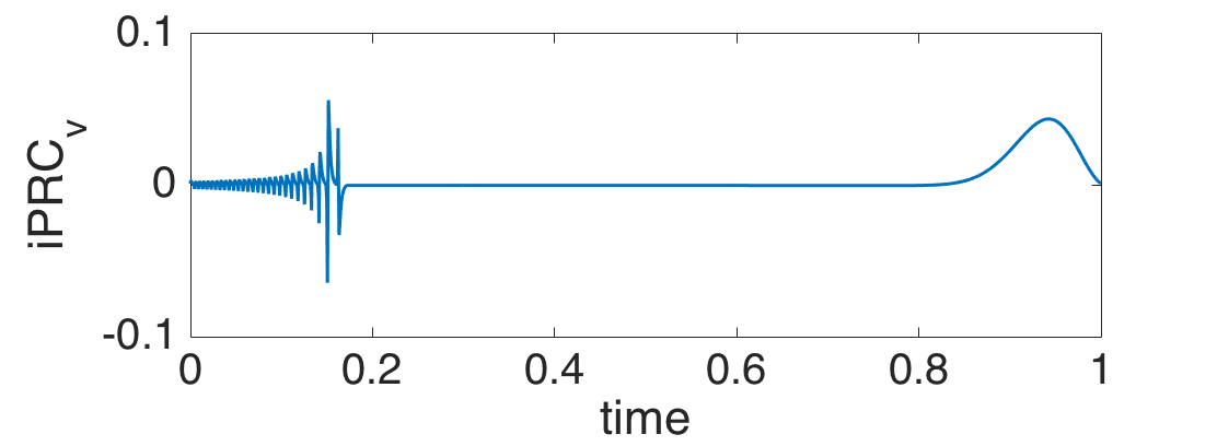
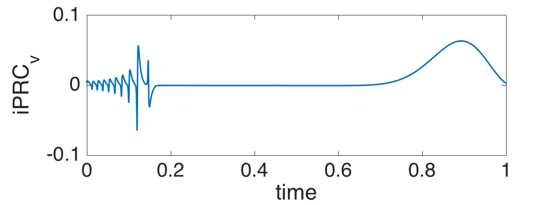
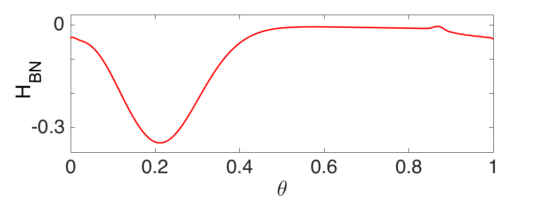
Figure 8: First row: iPRC (in the direction of $v$) for $\delta=0.0097$ (left), $\delta=0.03$ (right). Second row: the coupling functions $H_{BN}(\theta)$ for $\delta=0.0097$ (left), $\delta=0.03$ (right)

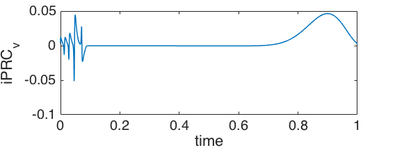
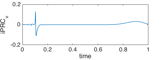
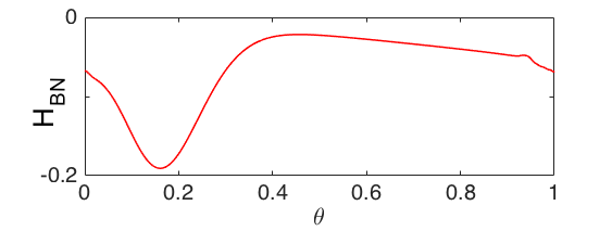
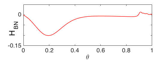
Figure 9: First row: iPRC (in the direction of $v$) for $I_{ext}=35.9$ (left), $I_{ext}=37.1$ (right). Second row: the coupling functions $H_{BN}(\theta)$ for $I_{ext}=35.9$ (left), $I_{ext}=37.1$ (right).

3.2 Phase equations for six weakly coupled neurons

We now apply the techniques from Section 3.1 to six coupled neurons and derive the 6-coupled phase oscillator model via phase reduction. We assume that all six hemi-segmental units have the same intrinsic (uncoupled) frequency $\omega$ and that the coupling functions $H_{i}$ are all identical ($H_{i}=H$) and T-periodic, $T=2\pi/\omega$. Recalling Equation (14) for a pair of neurons, this leads to the following system of ODEs describing the six legs’ motions.

$$\begin{array}[]{ll}&\dot{\phi}_{1}\;=\;\omega+{c}_{1}H(\phi_{4}-\phi_{1})+{c}_{5}H(\phi_{2}-\phi_{1}),\\ &\dot{\phi}_{2}\;=\;\omega+{c}_{2}H(\phi_{5}-\phi_{2})+{c}_{4}H(\phi_{1}-\phi_{2})+{c}_{7}H(\phi_{3}-\phi_{2}),\\ &\dot{\phi}_{3}\;=\;\omega+{c}_{3}H(\phi_{6}-\phi_{3})+{c}_{6}H(\phi_{2}-\phi_{3}),\\ &\dot{\phi}_{4}\;=\;\omega+{c}_{1}H(\phi_{1}-\phi_{4})+{c}_{5}H(\phi_{5}-\phi_{4}),\\ &\dot{\phi}_{5}\;=\;\omega+{c}_{2}H(\phi_{2}-\phi_{5})+{c}_{4}H(\phi_{4}-\phi_{5})+{c}_{7}H(\phi_{6}-\phi_{5}),\\ &\dot{\phi}_{6}\;=\;\omega+{c}_{3}H(\phi_{3}-\phi_{6})+{c}_{6}H(\phi_{5}-\phi_{6}).\end{array}$$ (17)

Oscillators 1, 2, and 3 drive the front, middle, and hind legs on the right with phases $\phi_{1},\phi_{2},$ and $\phi_{3}$, and oscillators 4, 5, and 6 drive the analogous legs on the left with phases $\phi_{4},\phi_{5},$ and $\phi_{6}$ ($\phi_{i}\in[0,T)$). Note that the derivation of the phase reduced system in Section 3.1 assumes that the coupling strength $\epsilon$ is small, implying that the product of the coefficients ${c}_{i}$ and $H$ in Equations (17) should be small compared to the uncoupled frequency $\omega$. Since $H$ includes $\bar{g}_{syn}$, (Equation (16)) and $\bar{g}_{syn}=0.01$, (Table 1), we have $H=\mathcal{O}(0.1)$ (Figures 8 and 9). In the examples studied below we will take ${c}_{i}=\mathcal{O}(1)$.

Next, we provide sufficient conditions such that an insect employs a tetrapod gait at low speeds and a tripod gait at high speeds. We first define idealized tetrapod and tripod gaits mathematically.

Definition 1 (Tetrapod and tripod gaits).

We define four versions of tetrapod gaits as follows. Each gait corresponds to a $T$-periodic solution of Equation (17). In each version two legs swing simultaneously in the sequences indicated in braces, and all six oscillators share the common coupled stepping frequency $\hat{\omega}$.

1. Forward right tetrapod gait $A_{FR},\{(R2,L3),(R1,L2),(R3,L1)\}$, corresponds to

   $$A_{FR}:=\left(\hat{\omega}t+\frac{2T}{3},\;\;\hat{\omega}t,\;\;\hat{\omega}t+\frac{T}{3};\;\;\hat{\omega}t+\frac{T}{3},\;\;\hat{\omega}t+\frac{2T}{3},\;\;\hat{\omega}t\right).$$

2. Forward left tetrapod gait $A_{FL},\{(R2,L1),(R1,L3),(R3,L2))\}$, corresponds to

   $$A_{FL}:=\left(\hat{\omega}t+\frac{2T}{3},\;\;\hat{\omega}t,\;\;\hat{\omega}t+\frac{T}{3};\;\;\hat{\omega}t,\;\;\hat{\omega}t+\frac{T}{3},\;\;\hat{\omega}t+\frac{2T}{3}\right).$$

3. Backward right tetrapod gait $A_{BR},\{(R2,L3),(R3,L1),(R1,L2)\}$, corresponds to

   $$A_{BR}:=\left(\hat{\omega}t+\frac{T}{3},\;\;\hat{\omega}t,\;\;\hat{\omega}t+\frac{2T}{3};\;\;\hat{\omega}t+\frac{2T}{3},\;\;\hat{\omega}t+\frac{T}{3},\;\;\hat{\omega}t\right).$$

4. Backward left tetrapod gait $A_{BL},\{(R2,L1),(R3,L2),(R1,L3)\}$, corresponds to

   $$A_{BL}:=\left(\hat{\omega}t+\frac{T}{3},\;\;\hat{\omega}t,\;\;\hat{\omega}t+\frac{2T}{3};\;\;\hat{\omega}t,\;\;\hat{\omega}t+\frac{2T}{3},\;\;\hat{\omega}t+\frac{T}{3}\right).$$

Finally the tripod gait $A_{Tri},\{(R1,L2,R3),(R2,L1,L3)\}$, corresponds to

$$A_{Tri}:=\left(\hat{\omega}t+\frac{T}{2},\;\;\hat{\omega}t,\;\;\hat{\omega}t+\frac{T}{2};\;\;\hat{\omega}t,\;\;\hat{\omega}t+\frac{T}{2},\;\;\hat{\omega}t\right).$$

The frequency $\hat{\omega}$ will be determined later in Proposition 2. Depending on the sign of the coupling, ${c}_{i}H$, $\hat{\omega}$ is either larger or smaller than $\omega.$ Since we assumed that all the connections are inhibitory, ${c}_{i}H(\phi)<0$ in the relevant range $[T/3,2T/3]$, and therefore $\hat{\omega}<\omega.$

Note that in both tetrapod and tripod gaits, the phase difference between the left and right legs in each segment is constant and is either equal to $T/3$ or $2T/3$ (in tetrapod gaits) or $T/2$ (in tripod gaits).

We would like to show that Equations (17) admit a stable solution at $A_{FR}$ or $A_{FL}$ corresponding to a forward right or left tetrapod gait, respectively, when the speed parameter ${\xi}$ (representing either $\delta$ or $I_{ext}$) is “small,” and a stable solution at $A_{Tri}$ corresponding to a tripod gait, when the speed parameter ${\xi}$ is “large.” Since we are interested in studying the effect of the speed parameter ${\xi}$ on gait transition, we let the coupling function $H$ and the frequency $\omega$ depend on ${\xi}$ and write $H=H(\phi;{\xi})$ and $\omega=\omega({\xi})$.

Definition 2 (Transition gaits).

For any fixed number ${\eta}\in[0,T/6]$, the forward right and forward left transition gaits, $A_{FR}({\eta})$ and $A_{FL}({\eta})$ respectively, are as follows.

$$A_{FR}({\eta}) :=\left(\hat{\omega}t+\frac{2T}{3}-{\eta},\;\hat{\omega}t,\;\hat{\omega}t+\frac{T}{3}+{\eta};\;\;\hat{\omega}t+\frac{T}{3}-2{\eta},\;\hat{\omega}t+\frac{2T}{3}-{\eta},\;\hat{\omega}t\right),$$ (18a)

$$A_{FL}({\eta}) :=\left(\hat{\omega}t+\frac{2T}{3}-{\eta},\;\hat{\omega}t,\;\hat{\omega}t+\frac{T}{3}+{\eta};\;\;\hat{\omega}t,\;\hat{\omega}t+\frac{T}{3}+{\eta},\;\hat{\omega}t+\frac{2T}{3}+2{\eta}\right).$$ (18b)

We call $A_{FR}({\eta})$ and $A_{FL}({\eta})$ “transition gaits” since as ${\eta}$ varies from $0$ to $T/6$, $A_{FR}({\eta})$ (resp. $A_{FL}({\eta})$) transits from the forward right (resp. left) tetrapod gait to the tripod gait. For ${\eta}=0$, $A_{FR}(0)=A_{FR}$ corresponds to the forward right tetrapod gait, and $A_{FL}(0)=A_{FL}$ corresponds to the forward left tetrapod gait. Also for ${\eta}=T/6$, $A_{FR}(T/6)=A_{FL}(T/6)=A_{Tri}$ corresponds to the tripod gait. In addition, the phase differences between the left and right legs ($\phi_{4}-\phi_{1},\phi_{5}-\phi_{2},\phi_{6}-\phi_{3}$), are constant and equal to $2T/3-{\eta}$ in $A_{FR}({\eta})$, and $T/3+{\eta}$ in $A_{FL}({\eta})$. This value is equal to $2T/3$ (resp. $T/3$) when ${\eta}=0$, as in the forward right (resp. left) tetrapod gait, and is equal to $T/2$, when ${\eta}=T/6$, as in the tripod gait.

We further assume that the phase differences between the left and right legs are equal to the steady state phase differences in $A_{FR}({\eta})$ or $A_{FL}({\eta})$ (later we will see that there are no differences between these two choices), i.e., we assume that for a fixed ${\eta}$, and for any $i=1,2,3$,

$$\phi_{i+3}=\phi_{i}+\bar{\phi}({\eta}),$$ (19)

where $\bar{\phi}({\eta})={2T}/{3}-{\eta}$ or $\bar{\phi}({\eta})={T}/{3}+{\eta}$. For steady states, this assumption is supported by experiments for tripod gaits [4], where $\bar{\phi}({\eta})=T/2$, and by simulations for tripod and tetrapod gaits in the bursting neuron model, Figures 6 and 7. We make a further simplifying assumption that the steady state contralateral phase differences remain constant for all $t$.

Thus, assuming that the phase difference between the left and right legs $\phi_{i+3}-\phi_{i}=\bar{\phi}({\eta})={2T}/{3}-{\eta}$ or $\bar{\phi}({\eta})={T}/{3}+{\eta}$, and noting that since $H=H(\phi;{\xi})$ is $T$-periodic in its first argument, $\phi_{i}-\phi_{i+3}=-\bar{\phi}({\eta})={T}/{3}+{\eta}\;\mbox{or}\;{2T}/{3}-{\eta}$ (recall that $-2T/3=T/3$ mod $T$), we can rewrite Equation (17) for the forward right transition gait $A_{FR}({\eta})$ as follows.

$$\dot{\phi}_{1}\;=\;\omega({\xi})+{c}_{1}H\left(\frac{2T}{3}-{\eta};{\xi}\right)+{c}_{5}H(\phi_{2}-\phi_{1};{\xi}),$$ (20a)

$$\dot{\phi}_{2}\;=\;\omega({\xi})+{c}_{2}H\left(\frac{2T}{3}-{\eta};{\xi}\right)+{c}_{4}H(\phi_{1}-\phi_{2};{\xi})+{c}_{7}H(\phi_{3}-\phi_{2};{\xi}),$$ (20b)

$$\dot{\phi}_{3}\;=\;\omega({\xi})+{c}_{3}H\left(\frac{2T}{3}-{\eta};{\xi}\right)+{c}_{6}H(\phi_{2}-\phi_{3};{\xi}),$$ (20c)

$$\dot{\phi}_{4}\;=\;\omega({\xi})+{c}_{1}H\left(\frac{T}{3}+{\eta};{\xi}\right)+{c}_{5}H(\phi_{5}-\phi_{4};{\xi}),$$ (20d)

$$\dot{\phi}_{5}\;=\;\omega({\xi})+{c}_{2}H\left(\frac{T}{3}+{\eta};{\xi}\right)+{c}_{4}H(\phi_{4}-\phi_{5};{\xi})+{c}_{7}H(\phi_{6}-\phi_{5};{\xi}),$$ (20e)

$$\dot{\phi}_{6}\;=\;\omega({\xi})+{c}_{3}H\left(\frac{T}{3}+{\eta};{\xi}\right)+{c}_{6}H(\phi_{5}-\phi_{6};{\xi}).$$ (20f)

A similar equation is obtained for $A_{FL}({\eta})$ as follows.

$$\dot{\phi}_{1}\;=\;\omega({\xi})+{c}_{1}H\left(\frac{T}{3}+{\eta};{\xi}\right)+{c}_{5}H(\phi_{2}-\phi_{1};{\xi}),$$ (21a)

$$\dot{\phi}_{2}\;=\;\omega({\xi})+{c}_{2}H\left(\frac{T}{3}+{\eta};{\xi}\right)+{c}_{4}H(\phi_{1}-\phi_{2};{\xi})+{c}_{7}H(\phi_{3}-\phi_{2};{\xi}),$$ (21b)

$$\dot{\phi}_{3}\;=\;\omega({\xi})+{c}_{3}H\left(\frac{T}{3}+{\eta};{\xi}\right)+{c}_{6}H(\phi_{2}-\phi_{3};{\xi}),$$ (21c)

$$\dot{\phi}_{4}\;=\;\omega({\xi})+{c}_{1}H\left(\frac{2T}{3}-{\eta};{\xi}\right)+{c}_{5}H(\phi_{5}-\phi_{4};{\xi}),$$ (21d)

$$\dot{\phi}_{5}\;=\;\omega({\xi})+{c}_{2}H\left(\frac{2T}{3}-{\eta};{\xi}\right)+{c}_{4}H(\phi_{4}-\phi_{5};{\xi})+{c}_{7}H(\phi_{6}-\phi_{5};{\xi}),$$ (21e)

$$\dot{\phi}_{6}\;=\;\omega({\xi})+{c}_{3}H\left(\frac{2T}{3}-{\eta};{\xi}\right)+{c}_{6}H(\phi_{5}-\phi_{6};{\xi}).$$ (21f)

Although we are interested in gait transitions in the bursting neuron model and in the phase reduction equations derived from the bursting neuron model, we prove our results for more general $H$. Our goal is to provide sufficient conditions on the coupling function $H$ and the coupling strengths ${c}_{i}$ that guarantee for any ${\eta}\in[0,T/6]$, $A_{FR}({\eta})$ or $A_{FL}({\eta})$ is a stable solution of Equations (20) and (21). To this end, in the following section we reduce the 6 equations (20a)-(20f) and the 6 equations (21a)-(21f) to 2 equations on a 2-torus. The coupling strengths ${c}_{i}$ may also depend on the speed parameter ${\xi}$ (see Section 7 below). For the rest of the paper, we assume that ${c}_{i}$ depends on ${\xi}$, ${c}_{i}={c}_{i}({\xi})$, but for simplicity, we drop the argument ${\xi}$.

3.3 Phase differences model

In this section, the goal is to reduce the 6 equations (20a)-(20f) and the 6 equations (21a)-(21f) to 2 equations on a 2-torus. To this end, we assume the following condition for the coupling function $H$.

Assumption 1.

Assume that $H=H(\theta;{\xi})$ is a differentiable function, defined on ${\mathbb{R}}\times{\color[rgb]{0,0,0}{[{\xi}_{1},{\xi}_{2}]}}$ which is $T$-periodic on its first argument and has the following property. For any fixed ${\xi}\in[{\xi}_{1},{\xi}_{2}]$,

$$H\left(\frac{2T}{3}-{\eta};{\xi}\right)=H\left(\frac{T}{3}+{\eta};{\xi}\right),$$ (22)

has a unique solution $\eta({\xi})$ such that $\eta=\eta({\xi}):[{\xi}_{1},{\xi}_{2}]\to[0,T/6]$ is an onto and non-decreasing function. Note that Equation (22) is also trivially satisfied by the constant solution ${\eta}=T/6$.

For the rest of the paper, we assume that the coupling function $H$ satisfies Assumption 1. In Proposition 9, Section 6, we characterize a class of functions $H$, that guarantee solutions of Equation (22). Also, we will show that the coupling functions $H_{BN}$ derived from the bursting neuron model satisfy Assumption 1, see Figures 8 and 9, and Section 5 below.

Using Equations (19) and (22), Equations (20) and (21) can be reduced to the following 3 equations describing the right legs’ motions:

$$\dot{\phi}_{1}\;=\;\omega({\xi})+{c}_{1}H\left(\frac{2T}{3}-{\eta};{\xi}\right)+{c}_{5}H(\phi_{2}-\phi_{1};{\xi}),$$ (23a)

$$\dot{\phi}_{2}\;=\;\omega({\xi})+{c}_{2}H\left(\frac{2T}{3}-{\eta};{\xi}\right)+{c}_{4}H(\phi_{1}-\phi_{2};{\xi})+{c}_{7}H(\phi_{3}-\phi_{2};{\xi}),$$ (23b)

$$\dot{\phi}_{3}\;=\;\omega({\xi})+{c}_{3}H\left(\frac{2T}{3}-{\eta};{\xi}\right)+{c}_{6}H(\phi_{2}-\phi_{3};{\xi}).$$ (23c)

Because only phase differences appear in the vector field, we may define

$$\theta_{1}:=\phi_{1}-\phi_{2}\quad\mbox{and}\quad\theta_{2}:=\phi_{3}-\phi_{2},$$

so that the following equations describe the dynamics of $\theta_{1}$ and $\theta_{2}$:

$$\dot{\theta}_{1}=({c}_{1}-{c}_{2})H\left(\frac{2T}{3}-{\eta};{\xi}\right)+{c}_{5}H(-\theta_{1};{\xi})-{c}_{4}H(\theta_{1};{\xi})-{c}_{7}H(\theta_{2};{\xi}),$$ (24a)

$$\dot{\theta}_{2}=({c}_{3}-{c}_{2})H\left(\frac{2T}{3}-{\eta};{\xi}\right)+{c}_{6}H(-\theta_{2};{\xi})-{c}_{4}H(\theta_{1};{\xi})-{c}_{7}H(\theta_{2};{\xi}).$$ (24b)

Note that Equations (24) are $T$-periodic in both variables, i.e., $(\theta_{1},\theta_{2})\in\mathbb{T}^{2}$, where $\mathbb{T}^{2}$ is a 2-torus.

In Equations (24), the tripod gait $A_{Tri}$ corresponds to the fixed point $(T/2,T/2)$, the forward tetrapod gaits, $A_{FR}$ and $A_{FL}$, correspond to the fixed point $(2T/3,T/3)$, and the transition gaits, $A_{FR}({\eta})$ and $A_{FL}({\eta})$, correspond to $(2T/3-{\eta},T/3+{\eta})$. Note that since $A_{FR}({\eta})$ and $A_{FL}({\eta})$ correspond to the same fixed point on the torus, we may assume the contralateral phase differences to be equal to $\phi_{i+3}-\phi_{i}={2T}/{3}-{\eta}$ or ${T}/{3}+{\eta}$. See [20] for another example of conditions on coupling functions that produce specific phase differences.

3.4 Qualitative behavior of the solutions of phase difference equations

In this section, as an example, we illustrate the nullclines and phase plane of Equations (24) with $H=H_{BN}$ and the coupling strengths as follows.

$${c}_{1}=1,\;{c}_{2}=2.5,\;{c}_{3}=1.5,\;{c}_{4}=5,\;{c}_{5}=7.5,\;{c}_{6}=7,\;{c}_{7}=1.$$ (25)

Here and henceforth, in all the simulations, we normalize the range of the coupling function $H_{BN}$ and so the torus is represented by a $1\times 1$ square. For example $(2T/3,T/3)$ is shown by a point at $(2/3,1/3)$, etc. To obtain phase portraits we solved Equations (24) using the fourth order Runge-Kutta method with fixed time step $0.001$ ms and ran the simulation up to 100 ms with multiple initial conditions.

Figure 10 (left to right) shows the nullclines and phase planes of Equations (24) with $H=H_{BN}$ computed in Figure 8(left), for a small $\delta=0.0097$ and Figure 8(right), for a large $\delta=0.03$, respectively. Intersections of the nullclines indicate the location of fixed points. We observe that for small $\delta$, the fixed points $(2/3,1/3)$ (corresponding to the forward tetrapod) and $(1/3,2/3)$ (corresponding to the backward tetrapod) are stable, while $(1/2,1/2)$ (corresponding to the tripod) is unstable. For larger $\delta$, the two tetrapod gaits merge to $(1/2,1/2)$, which becomes a sink.

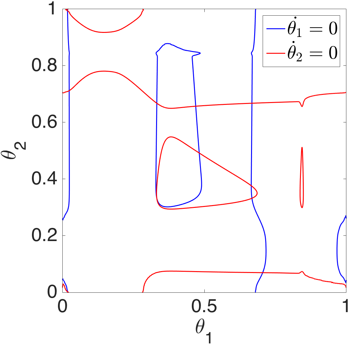
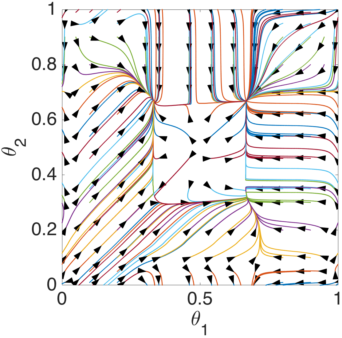
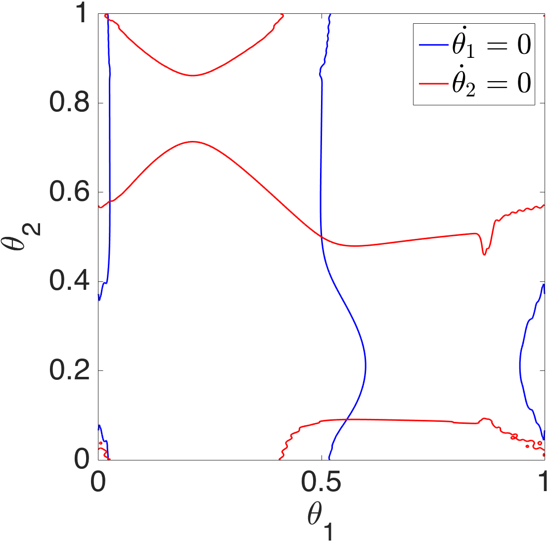
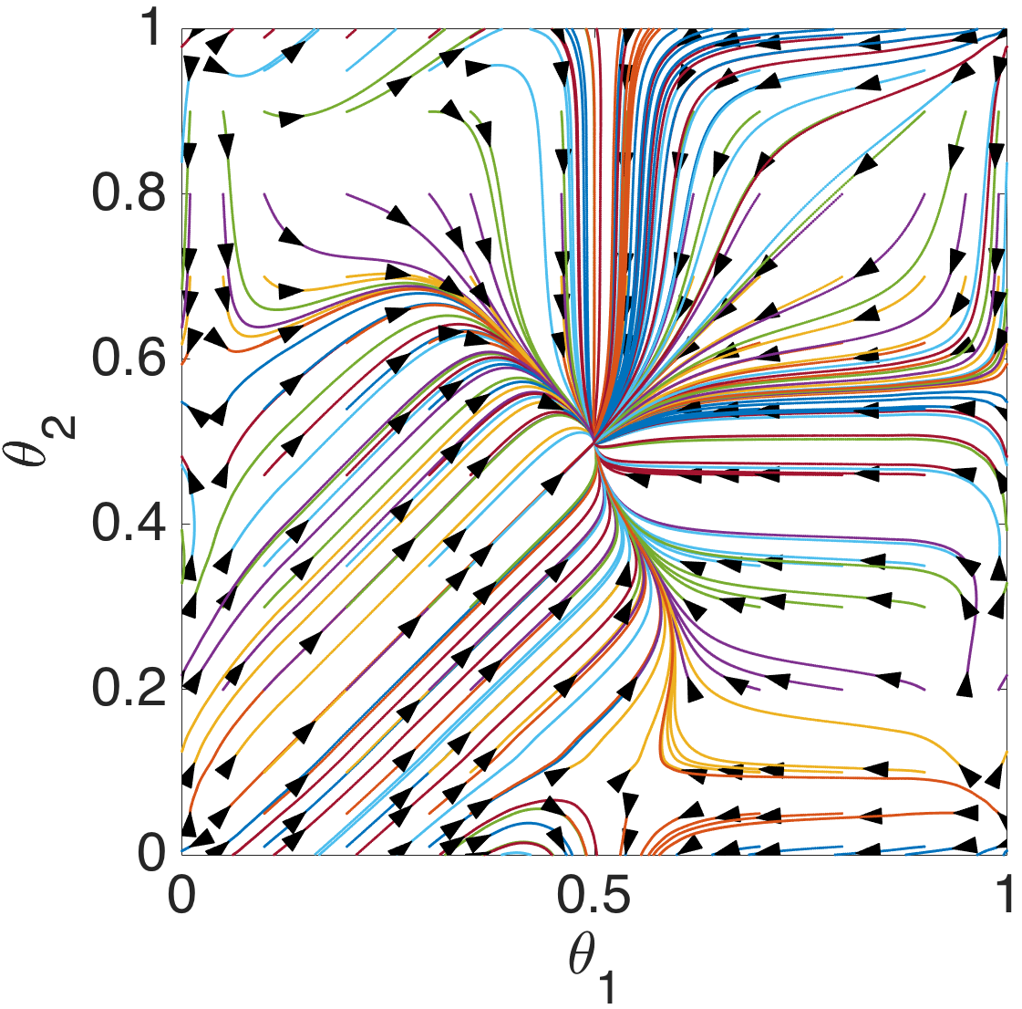
Figure 10: (Left to right) Nullclines and phase planes of Equations (24) when ${c}_{i}$’s satisfy Equation (25), and $\delta=0.0097$ and $0.03$, respectively. For computation of coupling functions, all bursting neuron parameters are as in the first rows of Table 1.

In the following sections we will address existence and stability of these fixed points and associated gaits and explore nonlinear phenomena involved in gait transitions.

4 Existence and stability of tetrapod and tripod gaits

We now prove that, under suitable conditions on the coupling functions and coupling strengths, multiple fixed points exist for Equations (24) and we derive explicit expressions for eigenvalues of the linearized system at these fixed points.

4.1 Existence with balance condition

We first provide conditions on the coupling strengths ${c}_{i}$ such that Equations (24) admit a stable fixed point at $(\theta_{1}^{1},\theta_{2}^{1}):=(2T/3-{\eta},T/3+{\eta})$, for any ${\eta}\in[0,T/6]$.

Proposition 1.

If the coupling strengths ${c}_{i}$ satisfy the following relations

$${c}_{1}+{c}_{5}={c}_{2}+{c}_{4}+{c}_{7}={c}_{3}+{c}_{6},$$ (26)

then for any ${\eta}\in[0,T/6]$, Equations (24) admit a fixed point at $(\theta_{1}^{1},\theta_{2}^{1})=(2T/3-{\eta},T/3+{\eta})$. Note that $(\theta_{1}^{1},\theta_{2}^{1})=(2T/3-{\eta},T/3+{\eta})$ corresponds to forward tetrapod (${\eta}=0$), forward transition ($0<{\eta}<T/6$), and tripod (${\eta}=T/6$) gaits. In addition, if the following inequalities hold, then the fixed point is stable.

$$\mbox{Tr}:=-({c}_{5}+{c}_{7})H^{\prime}\left(\frac{T}{3}+{\eta};{\xi}\right)-({c}_{4}+{c}_{6})H^{\prime}\left(\frac{2T}{3}-{\eta};{\xi}\right)<0,$$ (27a)

$$\mbox{Det}:={c}_{5}{c}_{6}H^{\prime}\left(\frac{T}{3}+{\eta};{\xi}\right)H^{\prime}\left(\frac{2T}{3}-{\eta};{\xi}\right)+{c}_{4}{c}_{6}\left[H^{\prime}\left(\frac{2T}{3}-{\eta};{\xi}\right)\right]^{2}+{c}_{5}{c}_{7}\left[H^{\prime}\left(\frac{T}{3}+{\eta};{\xi}\right)\right]^{2}>0.$$ (27b)

Equation (26) is called the balance equation; it expresses the fact that the sum of the coupling strengths entering each leg are equal. The equalities were assumed, without biological support, in [8], and were subsequently found to approximately hold for fast running cockroaches in [4, Figure 9c], according to the best data fits, judged by AIC and BIC, as reported in that paper.

Proof.

Since by Equation (22), $H({2T}/{3}-{\eta};{\xi})=H({T}/{3}+{\eta};{\xi})$, and

$$-(T/3+{\eta})=2T/3-{\eta}\quad\mbox{ mod $T$},$$

the right hand sides of Equations (24) at $(\theta_{1}^{1},\theta_{2}^{1})=(2T/3-{\eta},T/3+{\eta})$ are

$$({c}_{1}-{c}_{2}+{c}_{5}-{c}_{4}-{c}_{7})H\left(\frac{T}{3}+{\eta};{\xi}\right),$$ (28a)

$$({c}_{3}-{c}_{2}+{c}_{6}-{c}_{4}-{c}_{7})H\left(\frac{T}{3}+{\eta};{\xi}\right),$$ (28b)

which both are zero by Equations (26). Therefore, $(\theta_{1}^{1},\theta_{2}^{1})$ is a fixed point of Equations (24).

To study the stability of $(\theta_{1}^{1},\theta_{2}^{1})$, we consider the linearization of Equations (24) and evaluate the Jacobian of their right hand side at $(\theta_{1}^{1},\theta_{2}^{1})=(2T/3-{\eta},T/3+{\eta})$:

$$J_{1}\;=\;-\left(\begin{array}[]{ccc}{c}_{5}H^{\prime}\left(\frac{T}{3}+{\eta};{\xi}\right)+{c}_{4}H^{\prime}\left(\frac{2T}{3}-{\eta};{\xi}\right)&{c}_{7}H^{\prime}\left(\frac{T}{3}+{\eta};{\xi}\right)\\ \\ {c}_{4}H^{\prime}\left(\frac{2T}{3}-{\eta};{\xi}\right)&{c}_{6}H^{\prime}\left(\frac{2T}{3}-{\eta};{\xi}\right)+{c}_{7}H^{\prime}\left(\frac{T}{3}+{\eta};{\xi}\right)\end{array}\right),$$ (29)

where $H^{\prime}$ stands for the derivative $dH/d\theta$. A calculation shows that the trace and the determinant of $J_{1}$ at $(\theta_{1}^{1},\theta_{2}^{1})$ are as in Equation (27). Since $\mbox{Tr}<0$ and $\mbox{Det}>0$, both eigenvalues of $J_{1}$ have negative real parts and $(\theta_{1}^{1},\theta_{2}^{1})$ is a stable fixed point of Equations (24). ∎

Corollary 1.

Assume that $(\theta_{1}^{1},\theta_{2}^{1})=(2T/3-{\eta},T/3+{\eta})$ is a fixed point of Equations (24). Then,

• $(\theta_{1}^{2},\theta_{2}^{2})=(T/3+{\eta},T/3+{\eta})$,

• $(\theta_{1}^{3},\theta_{2}^{3})=(T/3+{\eta},2T/3-{\eta})$ which corresponds to a backward transition gait; and

• $(\theta_{1}^{4},\theta_{2}^{4})=(2T/3-{\eta},2T/3-{\eta})$,

are also fixed points of Equations (24).

Proof.

Since $-(T/3+{\eta})=2T/3-{\eta}$ mod $T$ and by Equation (22), $H({2T}/{3}-{\eta};{\xi})=H({T}/{3}+{\eta},;{\xi})$, the right hand sides of Equations (24) at $(\theta_{1}^{1},\theta_{2}^{1})=(2T/3-{\eta},T/3+{\eta})$ are equal to the right hand sides of Equations (24) at $(\theta_{1}^{i},\theta_{2}^{i})$, $i=2,3,4,$ and both are therefore equal to zero. ∎

Remark 2.

Besides the four fixed points $(\theta_{1}^{i},\theta_{2}^{i})$, $i=1,2,3,4,$ and depending on their stability types, Equations (24) may or may not admit more fixed points. By the Euler characteristic [21, Section 1.8], the sum of the indices of all the fixed points on a 2-torus must be zero; thus allowing us to infer the existence of additional fixed points.

Next we determine the coupled stepping frequency $\hat{\omega}$ such that the transition gaits defined in Equations (18) become solutions of Equations (20).

Proposition 2.

If the coupling strengths $c_{i}$ satisfy Equations (26) and (27), then for any ${\eta}\in[0,T/6]$, Equations (20) admit the following stable $T$-periodic solutions

$$A_{FR}({\eta}) :=\left(\hat{\omega}t+\frac{2T}{3}-{\eta},\;\hat{\omega}t,\;\hat{\omega}t+\frac{T}{3}+{\eta};\;\;\hat{\omega}t+\frac{T}{3}-2{\eta},\;\hat{\omega}t+\frac{2T}{3}-{\eta},\;\hat{\omega}t\right),$$ (30a)

$$A_{FL}({\eta}) :=\left(\hat{\omega}t+\frac{2T}{3}-{\eta},\;\hat{\omega}t,\;\hat{\omega}t+\frac{T}{3}+{\eta};\;\;\hat{\omega}t,\;\hat{\omega}t+\frac{T}{3}+{\eta},\;\hat{\omega}t+\frac{2T}{3}+2{\eta}\right),$$ (30b)

where the coupled stepping frequency $\hat{\omega}=\hat{\omega}({\xi})$, satisfies

$$\hat{\omega}=\omega({\xi})+({c}_{1}+{c}_{5})H\left(\frac{2T}{3}-{\eta};{\xi}\right)=\omega({\xi})+({c}_{2}+{c}_{4}+{c}_{7})H\left(\frac{2T}{3}-{\eta};{\xi}\right)=\omega({\xi})+({c}_{3}+{c}_{6})H\left(\frac{2T}{3}-{\eta};{\xi}\right).$$

Proof.

By the definition of $\hat{\omega}$, and using Equation (22), it can be seen that both $A_{FR}({\eta})$ and $A_{FL}({\eta})$ are $T$-periodic solutions of Equations (20). To check the stability of these solutions, we linearize the right hand side of Equations (20) at $A_{FR}({\eta})$ and $A_{FL}({\eta})$ to obtain

$$J_{2}=\left(\begin{array}[]{cc}A&0\\ 0&A\end{array}\right),$$

where $0$ represents a $3\times 3$ zero matrix and

$$A=\left(\begin{array}[]{ccccc}-{c}_{5}H^{\prime}\left(\frac{T}{3}+{\eta};\xi\right)&{c}_{5}H^{\prime}\left(\frac{T}{3}+{\eta};\xi\right)&0\\ \\ {c}_{4}H^{\prime}\left(\frac{2T}{3}-{\eta};\xi\right)&-{c}_{4}H^{\prime}\left(\frac{2T}{3}-{\eta};\xi\right)-{c}_{7}H^{\prime}\left(\frac{T}{3}+{\eta};\xi\right)&{c}_{7}H^{\prime}\left(\frac{T}{3}+{\eta};\xi\right)\\ \\ 0&{c}_{6}H^{\prime}\left(\frac{2T}{3}-{\eta};\xi\right)&-{c}_{6}H^{\prime}\left(\frac{2T}{3}-{\eta};\xi\right)\end{array}\right).$$

Note that since we assumed a constant contralateral symmetry between the right and left legs in Equations (20), these sets of legs are effectively decoupled and hence $J_{2}$ is a block diagonal matrix.

Some calculations show that the characteristic polynomial of $A$ is

$$g(\lambda)=-\lambda f(\lambda),$$

where

$$f(\lambda)=\lambda^{2}-\mbox{Tr}\lambda+\mbox{Det},$$

is the characteristic polynomial of $J_{1}$ (Equation (29)) and Tr and Det are defined in Equations (27). The non-zero eigenvalues of $A$ therefore have the same stability properties as the non-zero eigenvalues of $J_{2}$, and Equations (27) guarantee the stability of both $A_{FR}({\eta})$ and $A_{FL}({\eta})$, up to overall shifts in phase

$$\phi_{i}\rightarrow\phi_{i}+\bar{\phi}_{R},\quad\mbox{for}\;i=1,2,3,\qquad\mbox{and}\qquad\phi_{i}\rightarrow\phi_{i}+\bar{\phi}_{L},\quad\mbox{for}\;i=4,5,6,$$

that correspond to the two zero eigenvalues of $J_{2}$. ∎

Remark 3.

The balance condition Equation (26) is sufficient for the existence of tripod or tetrapod gaits. In Section 7, we will show the existence of such gaits for coupling strengths which approximate balance and also which are far from balance.

4.2 Existence with balance condition and equal contralateral couplings

In Proposition 1, we provided sufficient conditions for the stability of tetrapod gaits when the coupling strengths satisfy the balance condition, Equation (26).

In this section, in addition to the balance condition, we assume that ${c}_{1}={c}_{2}={c}_{3}$. Then under some extra conditions on ${c}_{i}$’s and $H$, we show that for any ${\eta}\in[0,T/6]$, the fixed point $(2T/3-{\eta},T/3+{\eta})$ is stable. The reason that we are interested in the assumption ${c}_{1}={c}_{2}={c}_{3}$ is the following estimated coupling strengths from fruit fly data [22]. We will return to this data set in Section 7.

$${c}_{1}=2.9145,\;{c}_{2}=2.5610,\;{c}_{3}=2.6160,\;{c}_{4}=2.9135,\;{c}_{5}=5.1800,\;{c}_{6}=5.4770,\;{c}_{7}=2.6165.$$

In this set of data, the ${c}_{i}$’s approximately satisfy the balance condition and also

$${c}_{1}\approx{c}_{2}\approx{c}_{3},\;{c}_{5}\approx{c}_{4}+{c}_{7}\approx{c}_{6}.$$

Proposition 3.

Assume that the coupling strengths ${c}_{i}$ satisfy Equation (26) and ${c}_{1}={c}_{2}={c}_{3}$. Also assume that $\forall{\eta}\in[0,T/6]$, $H^{\prime}=dH/d\theta$ satisfies

$$\quad H^{\prime}\left(\frac{T}{3}+\eta;{\xi}\right)+H^{\prime}\left(\frac{2T}{3}-\eta;{\xi}\right)>0.$$ (31)

Let $\alpha$ and $\alpha_{max}$ be as follows:

$$\alpha:=\frac{{c}_{4}}{{c}_{4}+{c}_{7}},\quad\alpha_{max}:=\frac{H^{\prime}\left(\frac{T}{3}+{\eta};{\xi}\right)}{H^{\prime}\left(\frac{T}{3}+{\eta};{\xi}\right)-H^{\prime}\left(\frac{2T}{3}-{\eta};{\xi}\right)}\;.$$ (32)

If

$$(\alpha_{max}-\alpha)\left(H^{\prime}\left(\frac{T}{3}+\eta;{\xi}\right)-H^{\prime}\left(\frac{2T}{3}-\eta;{\xi}\right)\right)>0,$$ (33)

then $(\theta_{1}^{1},\theta_{2}^{1})=(2T/3-{\eta},T/3+{\eta})$ is a stable fixed point of Equations (24) and if

$$(\alpha_{max}-\alpha)\left(H^{\prime}\left(\frac{T}{3}+\eta;{\xi}\right)-H^{\prime}\left(\frac{2T}{3}-\eta;{\xi}\right)\right)<0,$$ (34)

then $(\theta_{1}^{1},\theta_{2}^{1})=(2T/3-{\eta},T/3+{\eta})$ is a saddle point.

Proof.

Using the assumption ${c}_{1}={c}_{2}={c}_{3}$ and Equation (26), the following relations among the coupling strengths hold:

$${c}_{1}={c}_{2}={c}_{3},\;{c}_{5}={c}_{4}+{c}_{7}={c}_{6}.$$ (35)

Letting

$$\alpha:=\frac{{c}_{4}}{{c}_{4}+{c}_{7}},\quad(0<\alpha<1),$$ (36)

and making a change of time variable that eliminates ${c}_{5}$, Equations (24) become

$$\dot{\theta}_{1}=H(-\theta_{1};{\xi})-\alpha H(\theta_{1};{\xi})-(1-\alpha)H(\theta_{2};{\xi}),$$ (37a)

$$\dot{\theta}_{2}=H(-\theta_{2};{\xi})-\alpha H(\theta_{1};{\xi})-(1-\alpha)H(\theta_{2};{\xi}).$$ (37b)

Consider the linearization of Equation (37) at $(\theta_{1},\theta_{2})$:

$$J_{3}(\theta_{1},\theta_{2})\;=\;-\left(\begin{array}[]{ccc}H^{\prime}(-\theta_{1};{\xi})+{\alpha}H^{\prime}(\theta_{1};{\xi})&(1-{\alpha})H^{\prime}(\theta_{2};{\xi})\\ \\ {\alpha}H^{\prime}(\theta_{1};{\xi})&H^{\prime}(-\theta_{2};{\xi})+(1-{\alpha})H^{\prime}(\theta_{2};{\xi})\end{array}\right).$$

Standard calculations show that the eigenvalues of $J_{3}$ at $(\theta_{1}^{1},\theta_{2}^{1})=(2T/3-{\eta},T/3+{\eta})$ are

$$\lambda_{1}^{1}=-H^{\prime}\left(\frac{2T}{3}-{\eta};{\xi}\right)-H^{\prime}\left(\frac{T}{3}+{\eta};{\xi}\right),\quad\mbox{and}\quad\lambda_{2}^{1}=-(1-{\alpha})H^{\prime}\left(\frac{T}{3}+{\eta};{\xi}\right)-{\alpha}H^{\prime}\left(\frac{2T}{3}-{\eta};{\xi}\right).$$

By Equation (31), $H^{\prime}\left(\frac{2T}{3}-{\eta};{\xi}\right)+H^{\prime}\left(\frac{T}{3}+{\eta};{\xi}\right)>0$, hence $\lambda_{1}^{1}<0$. A calculation shows that $\lambda_{2}^{1}<0$ if $H^{\prime}\left(\frac{T}{3}+\eta;{\xi}\right)-H^{\prime}\left(\frac{2T}{3}-\eta;{\xi}\right)>0$ and ${\alpha}<{\alpha}_{max}$ or $H^{\prime}\left(\frac{T}{3}+\eta;{\xi}\right)-H^{\prime}\left(\frac{2T}{3}-\eta;{\xi}\right)<0$ and ${\alpha}>{\alpha}_{max}$. Therefore, if Inequality (33) holds, then $(\theta_{1}^{1},\theta_{2}^{1})=(2T/3-{\eta},T/3+{\eta})$ is a stable fixed point. Otherwise, $(\theta_{1}^{1},\theta_{2}^{1})=(2T/3-{\eta},T/3+{\eta})$ is a saddle point. ∎

In the following corollary, assuming that Equation (31) holds and $H^{\prime}\left({2T}/{3}-\eta;{\xi}\right)<0$, we verify the stability types of the other fixed points introduced in Corollary 1 (in Section 5 we will see that the coupling function computed for the bursting neuron model satisfies both of these assumptions):

Proposition 4.

Assume that for some ${\eta}\in[0,T/6]$, Equation (31) holds and $H^{\prime}\left({2T}/{3}-\eta;{\xi}\right)<0$. Then

1. $\left(\theta_{1}^{2},\theta_{2}^{2}\right)=(T/3+{\eta},T/3+{\eta})$ is a saddle point.

2. $\left(\theta_{1}^{3},\theta_{2}^{3}\right)=(T/3+{\eta},2T/3-{\eta})$, which corresponds to a backward tetrapod gait, is a sink if

   $$\alpha>{\alpha_{min}:=\frac{H^{\prime}\left(\frac{2T}{3}-{\eta};{\xi}\right)}{H^{\prime}\left(\frac{2T}{3}-{\eta};{\xi}\right)-H^{\prime}\left(\frac{T}{3}+{\eta};{\xi}\right)}}\;,$$ (38)

   and a saddle point if ${\alpha}_{min}>0$ and ${\alpha}<{\alpha}_{min}$.

3. $\left(\theta_{1}^{4},\theta_{2}^{4}\right)=(2T/3-{\eta},2T/3-{\eta})$ is a sink.

Proof.

Note that for any $i=1,\ldots,4$, the fixed point $\left(\theta_{1}^{i},\theta_{2}^{i}\right)$ either lies on the line $\theta_{1}=\theta_{2}$ or on the line $\theta_{1}=-\theta_{2}$.

1. The eigenvalues of $J_{3}$ at $\left(\theta_{1}^{2},\theta_{2}^{2}\right)=(T/3+{\eta},T/3+{\eta})$ are

   $$\lambda_{1}^{2}=-H^{\prime}(2T/3-{\eta};{\xi})-H^{\prime}(T/3+{\eta};{\xi})\quad\mbox{and}\quad\lambda_{2}^{2}=-H^{\prime}(2T/3-{\eta};{\xi}).$$

   By Equation (31), $\lambda_{1}^{2}<0$ and since we assumed $H^{\prime}(2T/3-{\eta};{\xi})<0$, $\lambda_{2}^{2}>0$. Therefore, independent of the choice of $\alpha$, $\left(\theta_{1}^{2},\theta_{2}^{2}\right)$ is always a saddle point.

2. The eigenvalues of $J_{3}$ at $\left(\theta_{1}^{3},\theta_{2}^{3}\right)=(T/3+{\eta},2T/3-{\eta})$ are

   $$\lambda_{1}^{3}=-H^{\prime}(2T/3-{\eta};{\xi})-H^{\prime}(T/3+{\eta};{\xi})\quad\mbox{and}\quad\lambda_{2}^{3}=-(1-{\alpha})H^{\prime}(2T/3-{\eta};{\xi})-{\alpha}H^{\prime}(T/3+{\eta};{\xi}).$$

   By Equation (31), $\lambda_{1}^{3}<0$. Since $H^{\prime}\left({2T}/{3}-\eta;{\xi}\right)<0$, for $\alpha>\alpha_{min}$, $\lambda_{2}^{3}<0$. Therefore, $(\theta_{1}^{3},\theta_{2}^{3})$ is a sink. Note that for $\alpha<\alpha_{min}$, $\lambda_{2}^{3}$ becomes positive and so $(\theta_{1}^{3},\theta_{2}^{3})$ becomes a saddle point.

3. The eigenvalues of $J_{3}$ at $(\theta_{1}^{4},\theta_{2}^{4})=(2T/3-{\eta},2T/3-{\eta})$ are

   $$\lambda_{1}^{4}=-H^{\prime}(2T/3-{\eta};{\xi})-H^{\prime}(T/3+{\eta};{\xi})\quad\mbox{and}\quad\lambda_{2}^{4}=-H^{\prime}(T/3+{\eta};{\xi}).$$

   $H^{\prime}(2T/3-{\eta};{\xi})+H^{\prime}(T/3+{\eta};{\xi})>0$ and $H^{\prime}(2T/3-{\eta};{\xi})<0$ imply that $H^{\prime}(T/3+{\eta};{\xi})>0$. Therefore, both eigenvalues are negative and independent of the choice of $\alpha$, $(\theta_{1}^{4},\theta_{2}^{4})$ is always a sink.

∎

On the other hand, if we assume that $H^{\prime}(2T/3-{\eta};{\xi})>0$, then all stable fixed points become saddle points and the saddle points become stable fixed points.

Proposition 5.

In addition to $\left(\theta_{1}^{i},\theta_{2}^{i}\right)$, $i=1,\ldots,4$, when ${c}_{1}={c}_{2}={c}_{3}$, Equations (24) admit the following fixed points.

1. $(\theta_{1}^{5},\theta_{2}^{5})=(T/2,T/2)$ is a fixed point and if $\exists\,{\xi}_{*}\in[{\xi}_{1},{\xi}_{2}]$ such that for ${\xi}<{\xi}_{*}$, $H^{\prime}\left({T}/{2};\xi\right)<0$, while for ${\xi}>{\xi}_{*}$, $H^{\prime}\left({T}/{2};\xi\right)>0$, then the fixed point $(T/2,T/2)$ changes its stability to a sink from a source as ${\xi}$ increases.

2. $\left(\theta_{1}^{6},\theta_{2}^{6}\right)=(0,0)$ is a fixed point and when $H^{\prime}(0;{\xi})<0$, it is a source.

Proof.

1. The eigenvalues of $J_{3}$ at $(T/2,T/2)$ are

   $$\lambda_{1}^{5}=-H^{\prime}(T/2;{\xi})\quad\mbox{and}\quad\lambda_{1}^{5}=-2H^{\prime}(T/2;{\xi}),$$

   so the stability depends on the sign of $H^{\prime}(T/2;{\xi})$, which by assumption is positive for ${\xi}<{\xi}_{*}$. Hence, for ${\xi}<{\xi}_{*}$, both eigenvalues are positive and $(\theta_{1}^{5},\theta_{2}^{5})$ is a source and for for ${\xi}>{\xi}_{*}$, both eigenvalues becomes negative and hence $(\theta_{1}^{5},\theta_{2}^{5})=(T/2,T/2)$ becomes a sink.

2. The eigenvalues of $J_{3}$ at $(0,0)$ are

   $$\lambda_{1}^{6}=-H^{\prime}(0;{\xi})\quad\mbox{and}\quad\lambda_{1}^{6}=-2H^{\prime}(0;{\xi}),$$

   so the stability depends on the sign of $H^{\prime}(0;{\xi})$, which we assumed is negative. Therefore, $(0,0)$ is a source.

∎

Note that as explained in Remark 2, by the Euler characteristic of zero for the 2-torus, there should exist more fixed points (e.g. saddle points).

Proposition 6.

If ${c}_{1}={c}_{3}$ and ${c}_{5}={c}_{6}$, then $\theta_{1}=\theta_{2}$ is an invariant line.

Proof.

Setting ${c}_{1}={c}_{3}$ and ${c}_{5}={c}_{6}$ in Equations (24), we conclude that $\dot{\theta}_{1}=\dot{\theta}_{2}$. Hence $\theta_{1}=\theta_{2}$ is invariant. ∎

Corollary 2.

Under the conditions of Proposition 3, $\theta_{1}=\theta_{2}$ is an invariant line. In addition, if ${c}_{4}={c}_{7}$, then the system is reflection symmetric with respect to $\theta_{1}=\theta_{2}$; i.e., if $(\dot{\theta}_{1},\dot{\theta}_{2})=(a,b)$ at $(\bar{\theta}_{1},\bar{\theta}_{2})$, then $(\dot{\theta}_{1},\dot{\theta}_{2})=(b,a)$ at $(\bar{\theta}_{2},\bar{\theta}_{1})$.

Proof.

Setting $(\theta_{1},\theta_{2})=(\bar{\theta}_{1},\bar{\theta}_{2})$ and $(\theta_{1},\theta_{2})=(\bar{\theta}_{2},\bar{\theta}_{1})$ in Equations (37) yields the result. ∎

In the following sections we first apply the results of this section to the coupling functions computed for the bursting neuron model (Section 5). Then, we characterize a class of functions $H$ which satisfies Assumption 1 (Section 6).

5 Application to the bursting neuron model

In Section 3.1, for some $\delta$ and $I_{ext}$ values, we numerically computed the coupling function $H_{BN}$ for the bursting neuron model (see Figures 8 and 9). Here we show that the results of Section 4 apply to the coupling function $H_{BN}$.

Lemma 1.

The coupling function $H_{BN}$, which is computed numerically from the bursting neuron model, satisfies Assumption 1.

Proof.

Figure 11 shows the graphs of ${\eta}={\eta}({\xi})$, the solutions of Equation (22) for $H=H_{BN}$, where ${\xi}=\delta\in{\color[rgb]{0,0,0}{[\delta_{1},\delta_{2}]}}=[0.0097,0.04]$ (left) and ${\xi}=I_{ext}\in{\color[rgb]{0,0,0}{[I_{1},I_{2}]}}=[35.65,37.7]$ (right). (Note that solving Equation (22) is equivalent to solving $G_{BN}(\theta;{\xi})=0$ for $\theta$, where $G_{BN}(\theta;{\xi}):=H_{BN}(\theta;{\xi})-H_{BN}(-\theta;{\xi})$.) Note that ${\eta}$ is the unique solution of Equation (22) which is non-decreasing and onto. Therefore, Assumption 1 is satisfied.

Figure 11: The solution ${\eta}({\xi})$ of $H_{BN}\left({2T}/{3}-{\eta};{\xi}\right)=H_{BN}\left({T}/{3}+{\eta};{\xi}\right)$ where ${\xi}=\delta$ and ${\eta}:[0.0097,0.04]\to[0,1/6]$ (left); and where ${\xi}=I_{ext}$ and ${\eta}:[35.65,37.7]\to[0,1/6]$ (right).

∎

5.1 Balance condition

Since $H_{BN}$ satisfies Assumption 1, one can apply Proposition 1 to show that under balance condition for the coupling strengths, and Equations (27), $(2T/3-{\eta},T/3+{\eta})$ is a stable fixed point of Equation (24) with $H=H_{BN}$. In Section 3.4, Figure 10, we showed the nullclines and phase planes of Equations (24) with coupling strengths given in Equation (25). Note that those coupling strengths satisfy the balance equation and for $\delta=0.0097$, they satisfy Equations (27) (Tr $\approx-2.78<0$ and Det $\approx 0.61>0$). In Figure 10 (left to right) we observe that for small $\delta$, there exist 3 sinks corresponding to $(\theta_{1}^{i},\theta_{2}^{i})$, $i=1,3,4$, and 1 saddle point corresponding to $(\theta_{1}^{2},\theta_{2}^{2})$. In addition, there exist 2 sources (one located at $(1/2,1/2)$ and the other one at $(0,0)$), and $4$ more saddle points. When $\delta$ is large, for $i=1,2,3,4$, $(\theta_{1}^{i},\theta_{2}^{i})$ merge to $(1/2,1/2)$, and $(1/2,1/2)$, which corresponds to the tripod gait, becomes a sink. The unstable fixed point $(0,0)$ and the two remaining saddle points, near the boundary, preserve their stability types.

5.2 Balance condition and equal contralateral couplings

In this section we apply Proposition 3 to $H_{BN}$ to show existence and stability of tetrapod and tripod gaits.

Proposition 7.

Consider Equations (37) for $H=H_{BN}$. If $\alpha<\alpha_{max}$ (as defined in Equation (32)), then $(\theta_{1}^{1},\theta_{2}^{1})=(2T/3-{\eta},T/3+{\eta})$ is a stable fixed point of Equations (24) and if $\alpha>\alpha_{max}$ then $(\theta_{1}^{1},\theta_{2}^{1})=(2T/3-{\eta},T/3+{\eta})$ is a saddle point.

Proof.

Figure 12 shows that $H_{BN}^{\prime}(2T/3-{\eta};{\xi})+H_{BN}^{\prime}(T/3+{\eta};{\xi})>0$, for ${\xi}=\delta$ and ${\xi}=I_{ext}$. Hence, Equation (31) holds.

Figure 12: $\lambda_{1}^{1}=-H_{BN}^{\prime}(2T/3-{\eta};{\xi})-H_{BN}^{\prime}(T/3+{\eta};{\xi})$ vs. ${\xi}=\delta$ (left) and $\xi=I_{ext}$ (right) are shown.

Figure 13 shows that $H_{BN}^{\prime}(2T/3-{\eta};{\xi})<0$ and $H_{BN}^{\prime}(T/3+{\eta};{\xi})>0$. Therefore, $H_{BN}^{\prime}(T/3+{\eta};{\xi})-H_{BN}^{\prime}(2T/3-{\eta};{\xi})>0$. Hence, by Proposition 3, If $\alpha<\alpha_{max}$, Equation (33) holds and $(\theta_{1}^{1},\theta_{2}^{1})=(2T/3-{\eta},T/3+{\eta})$ is a stable fixed point of Equations (24) and if $\alpha>\alpha_{max}$, Equation (34) holds and $(\theta_{1}^{1},\theta_{2}^{1})=(2T/3-{\eta},T/3+{\eta})$ is a saddle point.

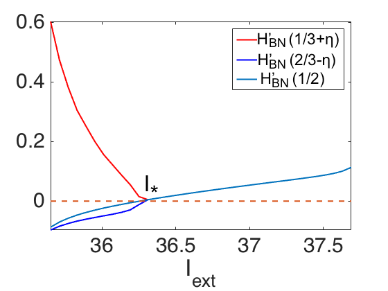
Figure 13: $H_{BN}^{\prime}(2T/3-{\eta};{\xi})$, $H_{BN}^{\prime}(T/3+{\eta};{\xi})$, and $H_{BN}^{\prime}(T/2;{\xi})$ vs. ${\xi}=\delta$ (left) and ${\xi}=I_{ext}$ (right) are shown. Note that the curves first meet at $\delta_{*}$ (left) and $I_{*}$ (right) and subsequently overlap for $\delta>\delta_{*}$ and $I_{ext}>I_{*}$.

∎

Moreover, we apply Propositions 4 and 5 to show the existence and stability of more fixed points.

Proposition 8.

In Equations (37) with $H=H_{BN}$:

1. $\left(\theta_{1}^{2},\theta_{2}^{2}\right)=(T/3+{\eta},T/3+{\eta})$ is a saddle point.

2. If $\alpha>\alpha_{min}$ (as defined in Equation (38)), then $(\theta_{1}^{3},\theta_{2}^{3})=(T/3+{\eta},2T/3-{\eta})$ is a stable fixed point, otherwise, it is a saddle point.

3. $\left(\theta_{1}^{4},\theta_{2}^{4}\right)=(2T/3-{\eta},2T/3-{\eta})$ is a sink.

4. For ${\xi}<{\xi}_{*}$ (${\xi}_{*}=\delta_{*}\approx 0.0208$ and ${\xi}_{*}=I_{*}\approx 36.3$), $(T/2,T/2)$ is a source and for ${\xi}>{\xi}_{*}$, $(T/2,T/2)$ becomes a sink.

Proof.

By Figure 12, $H_{BN}^{\prime}(2T/3-{\eta};{\xi})+H_{BN}^{\prime}(T/3+{\eta};{\xi})>0$ and by Figure 13, $H_{BN}^{\prime}(2T/3-{\eta};{\xi})<0$, and $H_{BN}^{\prime}(T/2;{\xi})$ changes sign from negative to positive at ${\xi}={\xi}_{*}$ (${\xi}_{*}=\delta_{*}\approx 0.0208$ and ${\xi}_{*}=I_{*}\approx 36.3$). Therefore, Propositions 4 and 5 give the desired results. ∎

5.3 Phase plane analyses

We now study Equations (37) by analyzing phase planes. In the following cases we preserve the balance condition and let ${c}_{1}={c}_{2}={c}_{3}$, but allow $\alpha$ to vary. First we assume that $\alpha=1/2$ (rostrocaudal symmetry), for which, by Corollary 2, the system is reflection symmetric with respect to $\theta_{1}=\theta_{2}$. For example, we let

$${c}_{1}={c}_{2}={c}_{3}=0.5,\;{c}_{4}={c}_{7}=1,\;{c}_{5}={c}_{6}=2.$$

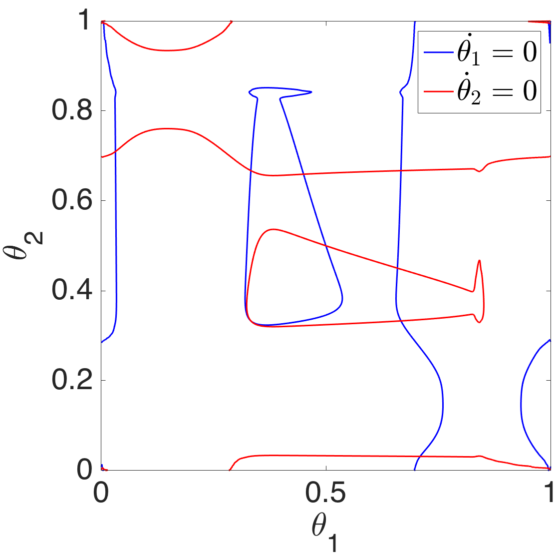
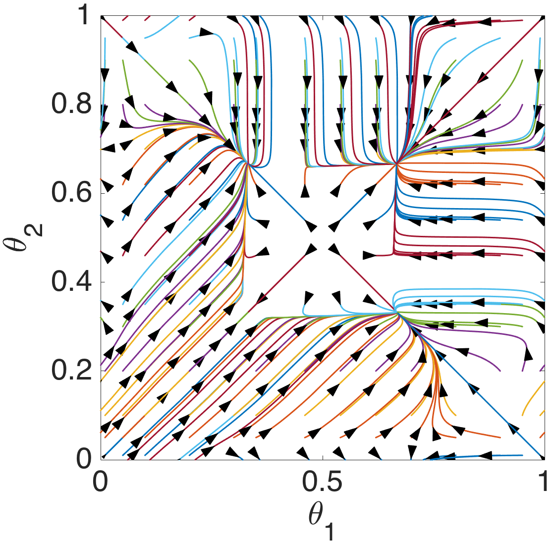
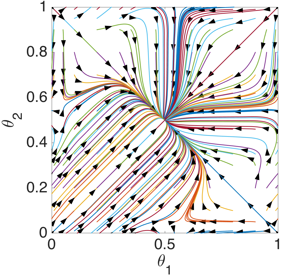
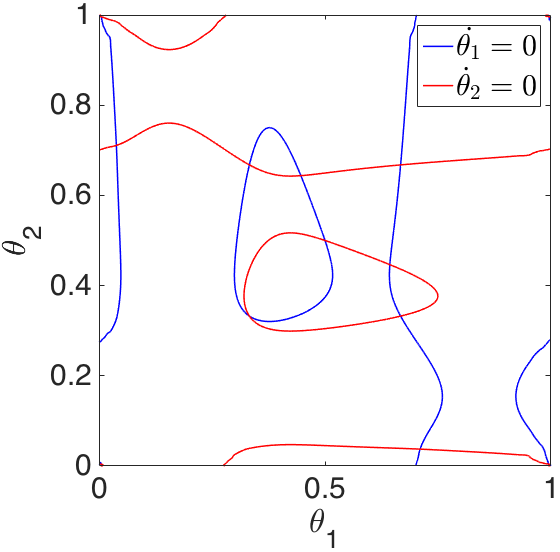
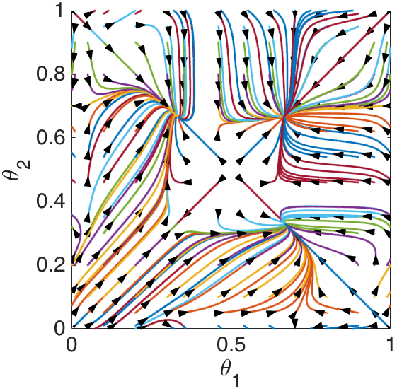
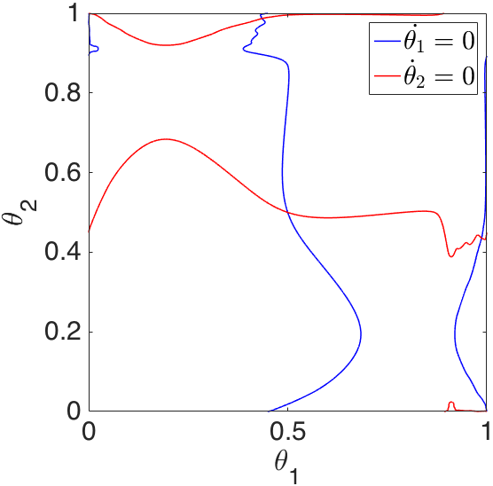
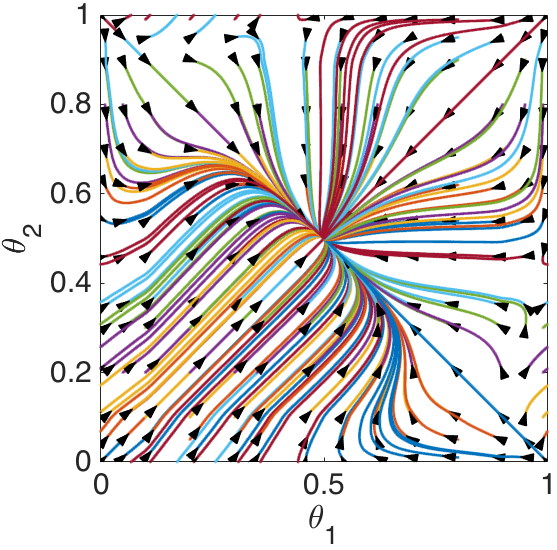
Figure 14: Nullclines and phase planes of Equation (37) when $\alpha=1/2$. First row: $\delta=0.0097$ (left) and $\delta=0.03$ (right). Second row: $I_{ext}=35.65$ (left) and $I_{ext}=37.1$ (right). Note reflection symmetry.

Figure 14 (first row, left to right) shows the nullclines and phase planes of Equations (37), for a small $\delta=0.0097<\delta_{*}$, and a large $\delta=0.03>\delta_{*}$, respectively. Figure 14 (second row, left to right) shows the nullclines and phase planes of Equations (37), for a small $I_{ext}=35.65<I_{*}$ and a large $I_{ext}=37.1>I_{*}$, respectively. As expected from Proposition 3 and Proposition 4, we observe that when $\delta$ or $I_{ext}$ is small, there exist 3 sinks corresponding to $(\theta_{1}^{i},\theta_{2}^{i})$, $i=1,3,4$, and 2 sources corresponding to $(\theta_{1}^{i},\theta_{2}^{i})$, $i=5,6$. In addition, there exist $5$ saddle points, of which one corresponds to $(\theta_{1}^{2},\theta_{2}^{2})$. When $\delta$ or $I_{ext}$ is large, $(\theta_{1}^{i},\theta_{2}^{i})$, for $i=1,2,3,4$ merge to $(\theta_{1}^{5},\theta_{2}^{5})=(1/2,1/2)$, and we observe that $(1/2,1/2)$ which corresponds to the tripod gait, becomes a sink. The unstable fixed point $(0,0)$ and two saddle points continue to exist and preserve their stability types.

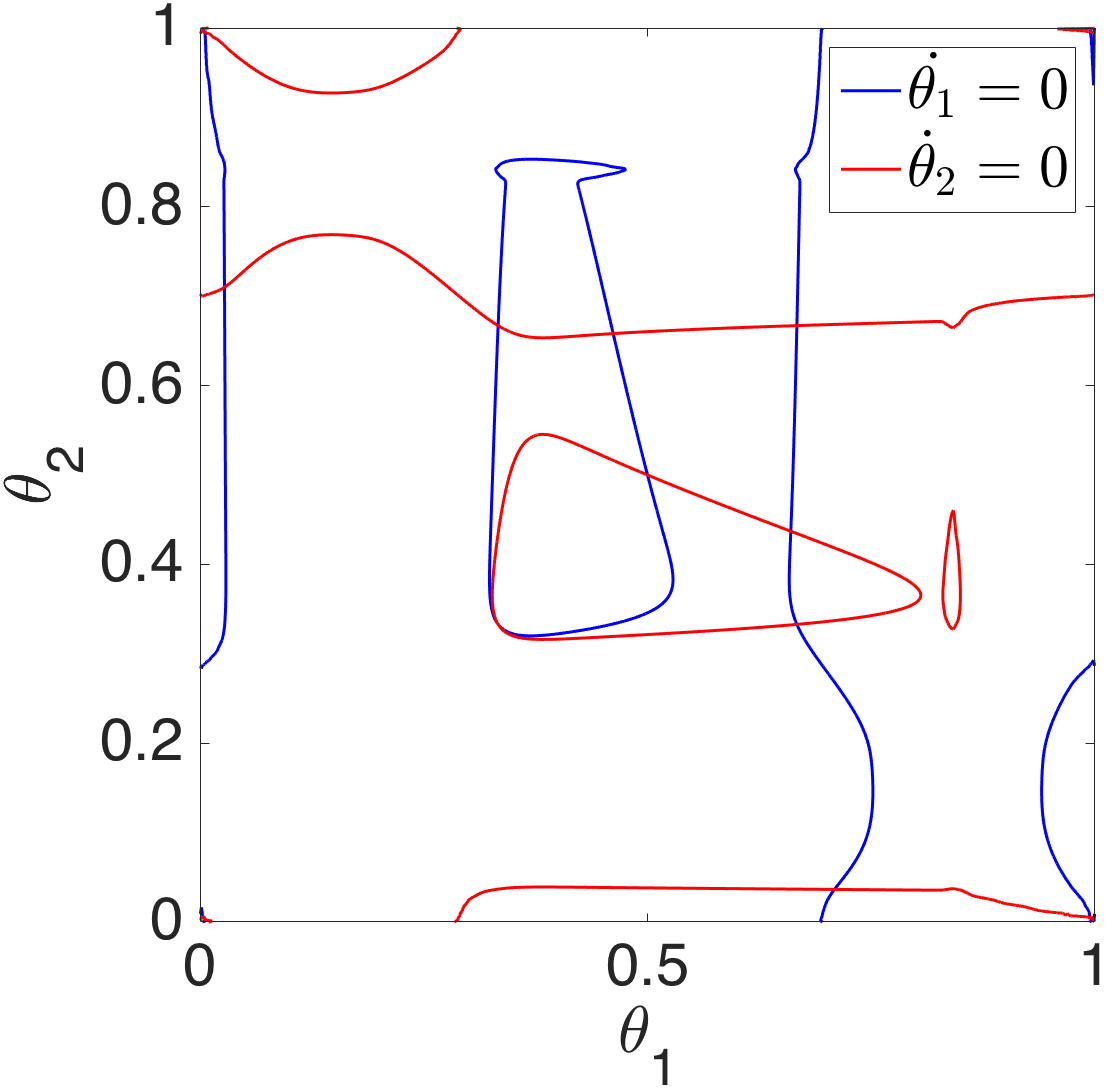
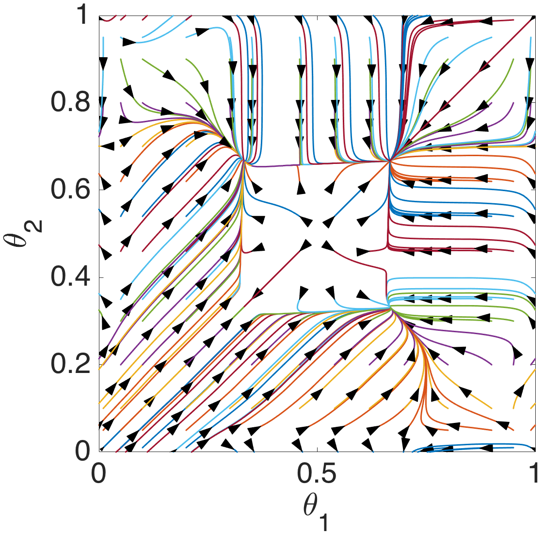
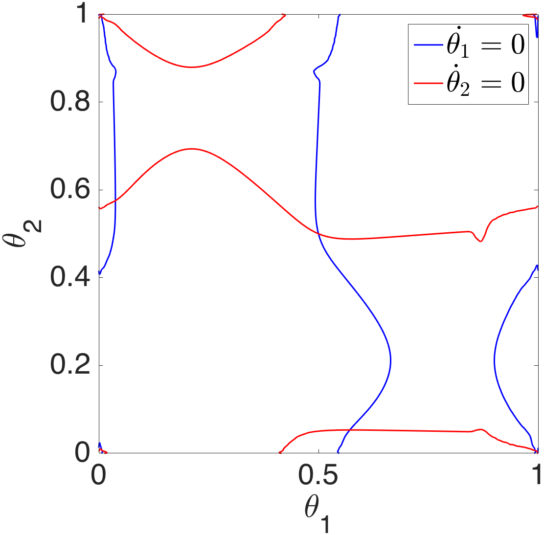
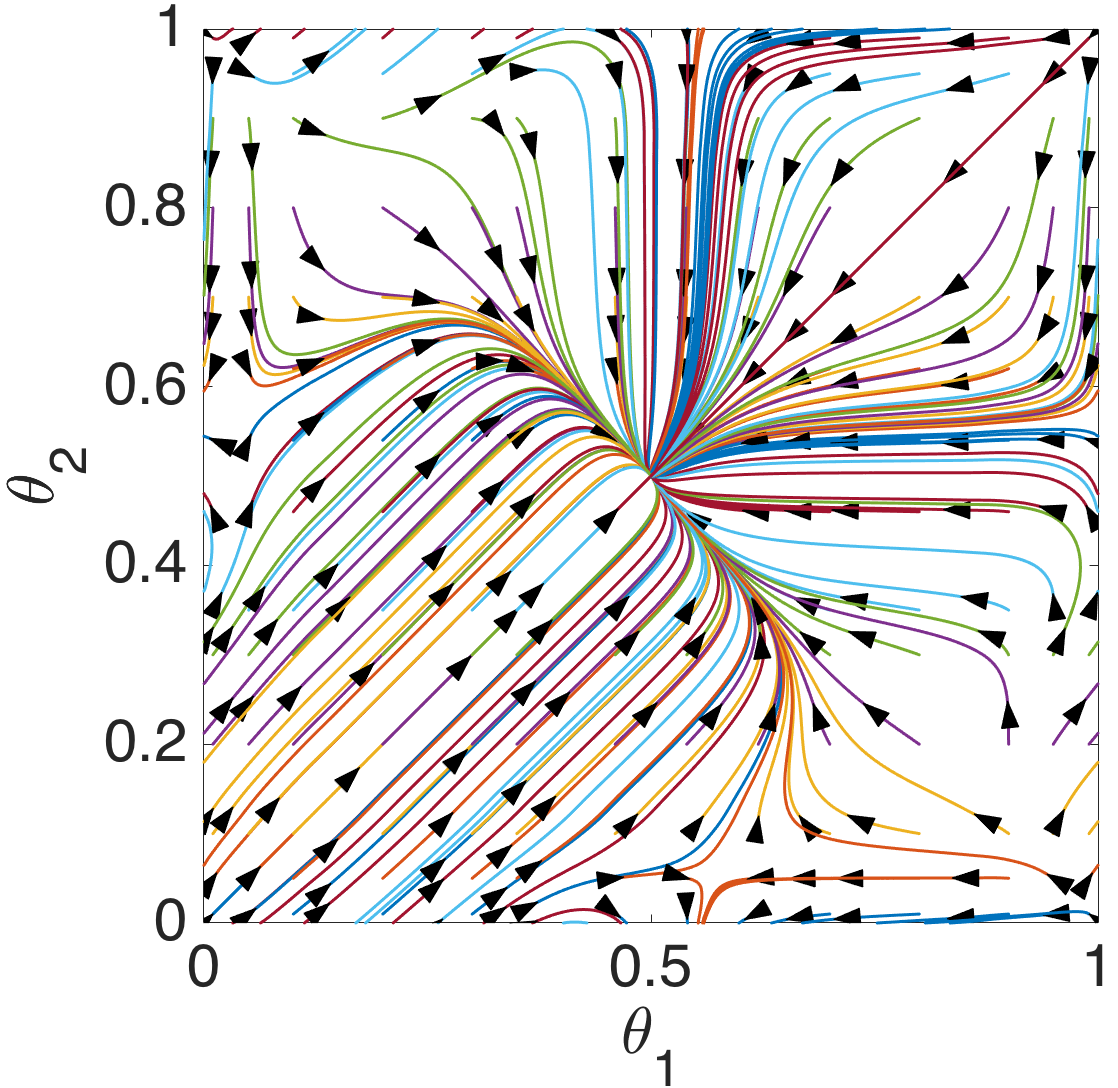
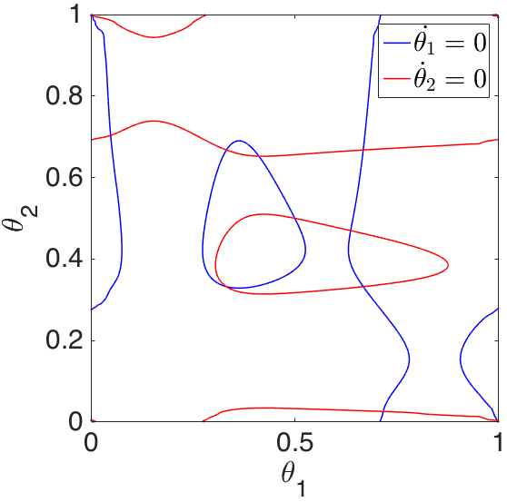
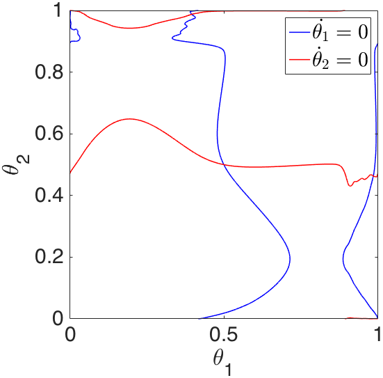
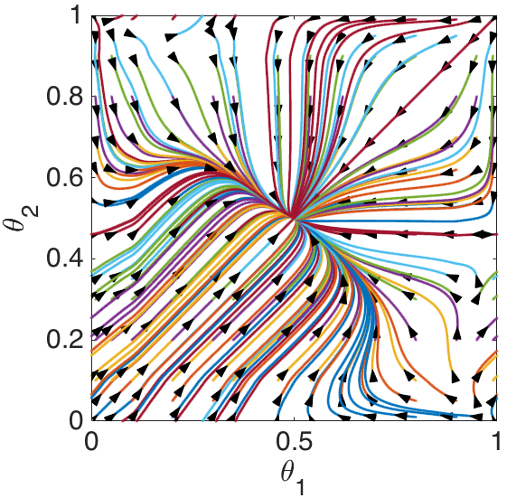
Figure 15: Nullclines and phase planes of Equations (37) when $\alpha=1/3$. First row: $\delta=0.0097$ (left) and $\delta=0.03$ (right). Second row: $I_{ext}=35.65$ (left) and $I_{ext}=37.1$ (right). Reflection symmetry is slightly broken, but the invariant line $\theta_{1}=\theta_{2}$ persists.

Next, we let ${\alpha}\neq 1/2$ but keep it close to $1/2$, i.e., we want $\alpha_{min}<\alpha<\alpha_{max}$. Specifically, we set

$${c}_{1}={c}_{2}={c}_{3}={c}_{4}=1,\;{c}_{7}=2,\;{c}_{5}={c}_{6}=3,$$

so that ${\alpha}=1/3$. Figure 15 (first row, left to right) shows the nullclines and the phase planes of Equations (37), for a small $\delta=0.0097$, and a large $\delta=0.03$, respectively. Figure 15 (second row, left to right) shows the nullclines and the phase planes of Equations (37), for a small $I_{ext}=35.65$ and a large $I_{ext}=37.1$, respectively. As we expect, the qualitative behaviors of the fixed points do not change, but reflection symmetry about the diagonal $\theta_{1}=\theta_{2}$ is broken, most easily seen in the nullclines.

Finally, we let ${\alpha}\approx 1$, i.e., $\alpha>\alpha_{max}$. For $\delta<\delta_{*}$ (resp. $I_{ext}<I_{*}$), we expect to have a stable backward tetrapod gait at $(T/3+{\eta},2T/3-{\eta})$ and an unstable forward tetrapod gait at $(2T/3-{\eta},T/3+{\eta})$. For $\delta>\delta_{*}$ (resp. $I_{ext}>I_{*}$), the tripod gait at $(T/2,T/2)$ becomes stable. In the simulations shown below we let

$${c}_{1}={c}_{2}={c}_{3}=0.5,\;{c}_{4}=2,\;{c}_{7}=0.1,\;{c}_{5}={c}_{6}=2.1,$$

so that ${\alpha}\approx 0.952.$

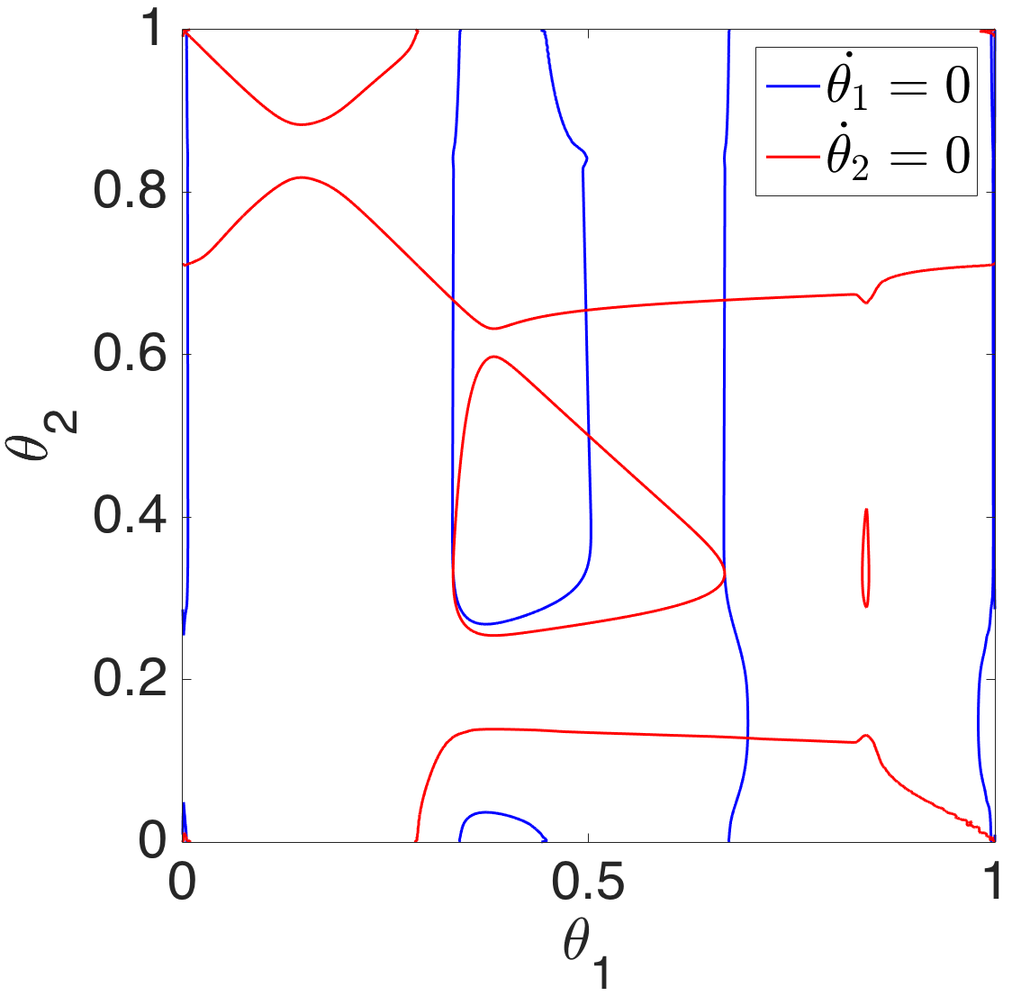
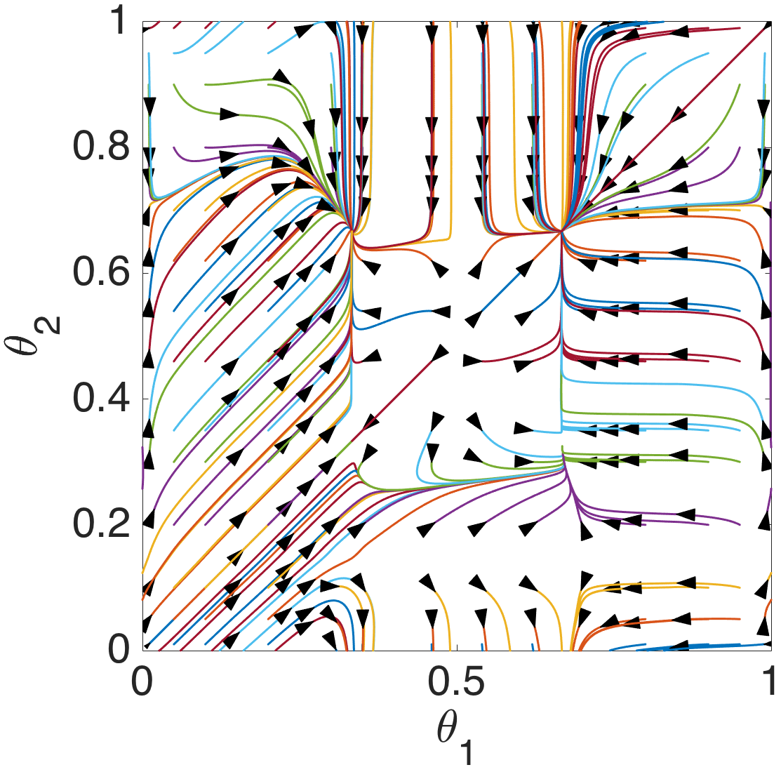
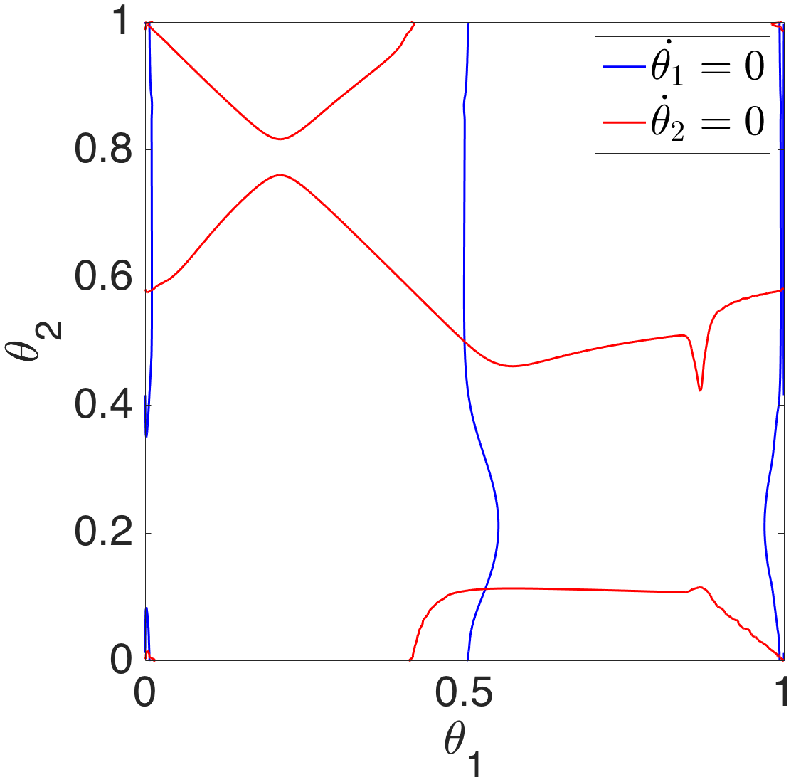
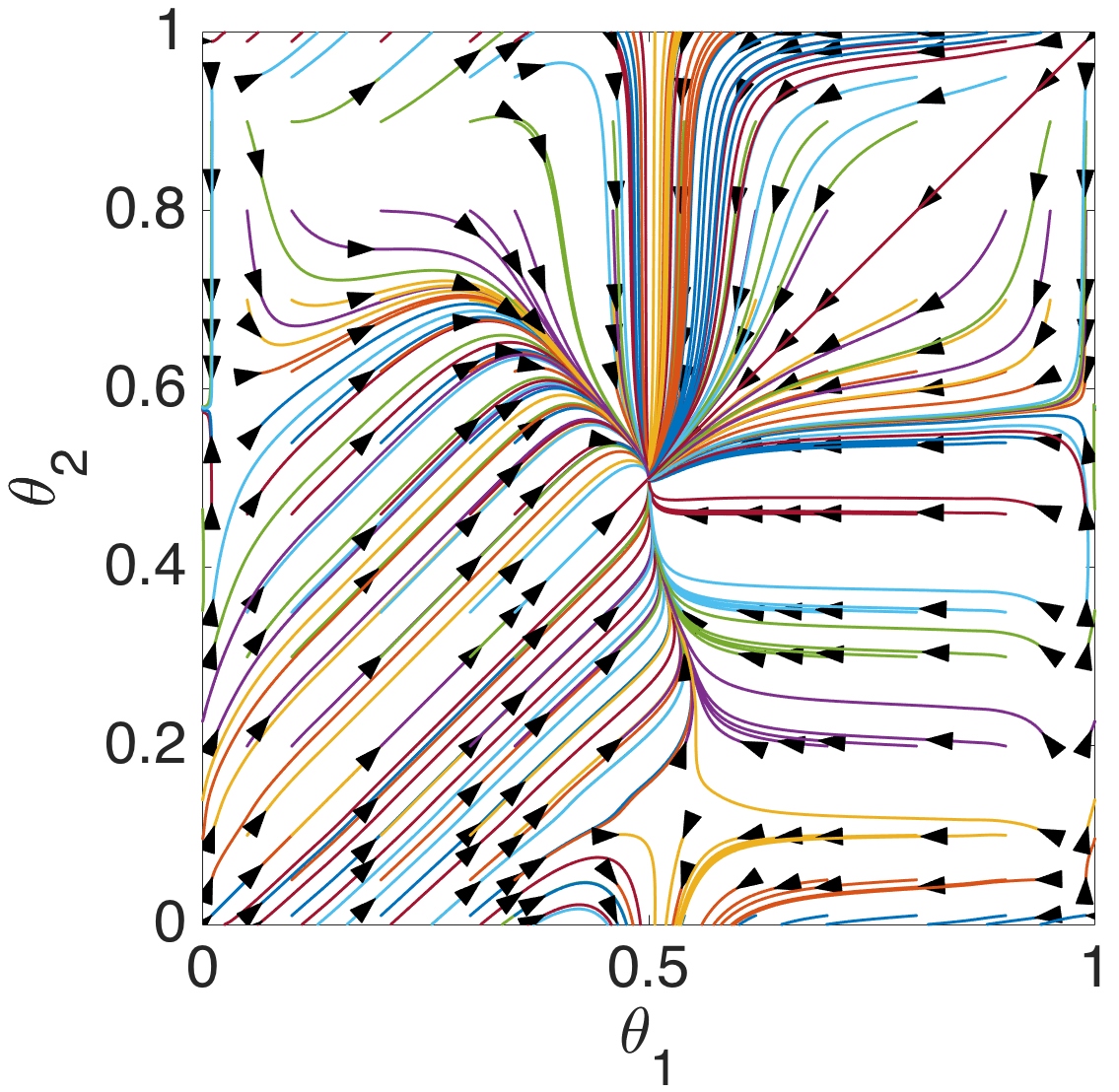
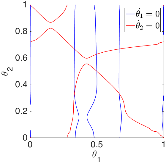
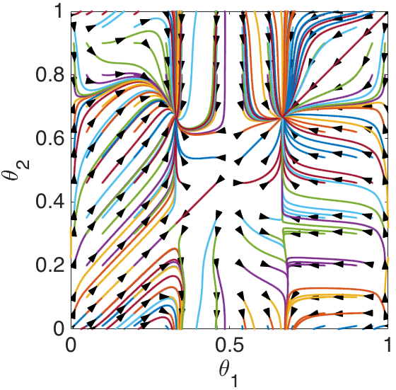
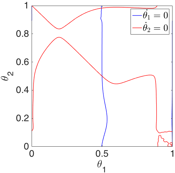
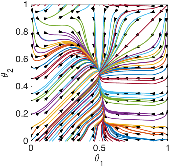
Figure 16: Nullclines and phase planes of Equations (37) when $\alpha\approx 0.95>{\alpha}_{max}$. First row: $\delta=0.0097$ (left) and $\delta=0.03$ (right). Second row: $I_{ext}=35.65$ (left) and $I_{ext}=37.1$ (right). Reflection symmetry is clearly broken.

Figure 16 (first row, left to right) shows the nullclines and phase planes of Equation (37) for a small $\delta=0.0097$, and a large $\delta=0.03$, respectively. Figure 16 (second row, left to right) shows the nullclines and the phase planes of Equation (37), for a small $I_{ext}=35.65$ and a large $I_{ext}=37.1$, respectively. Here reflection symmetry is broken more obviously. Similarly, when ${\alpha}$ is near zero, i.e., $\alpha<\alpha_{min}$, we expect to have a stable forward tetrapod gait, and an unstable backward tetrapod gait. In Figure 17, we let ${c}_{1}={c}_{2}={c}_{3}=0.5,\;{c}_{4}=0.1,\;{c}_{7}=3,\;{c}_{5}={c}_{6}=3.1,$ so that ${\alpha}\approx 0.032.$ As we expect, the forward tetrapod gait remains stable while the backward tetrapod gait becomes a saddle through a transcritical bifurcation. However, a stable fixed point appears (through the same transcritical bifurcation) very close to the backward tetrapod gait.

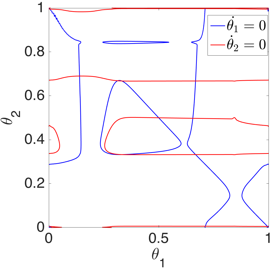
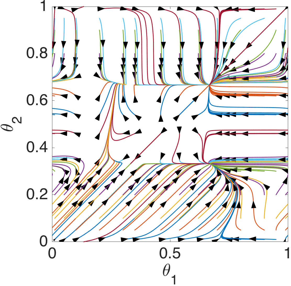
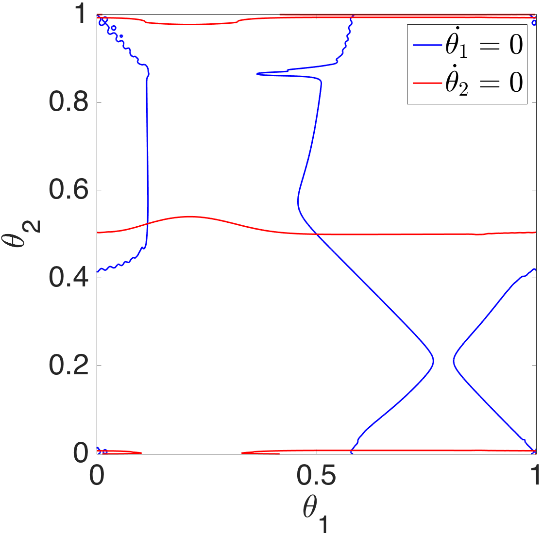
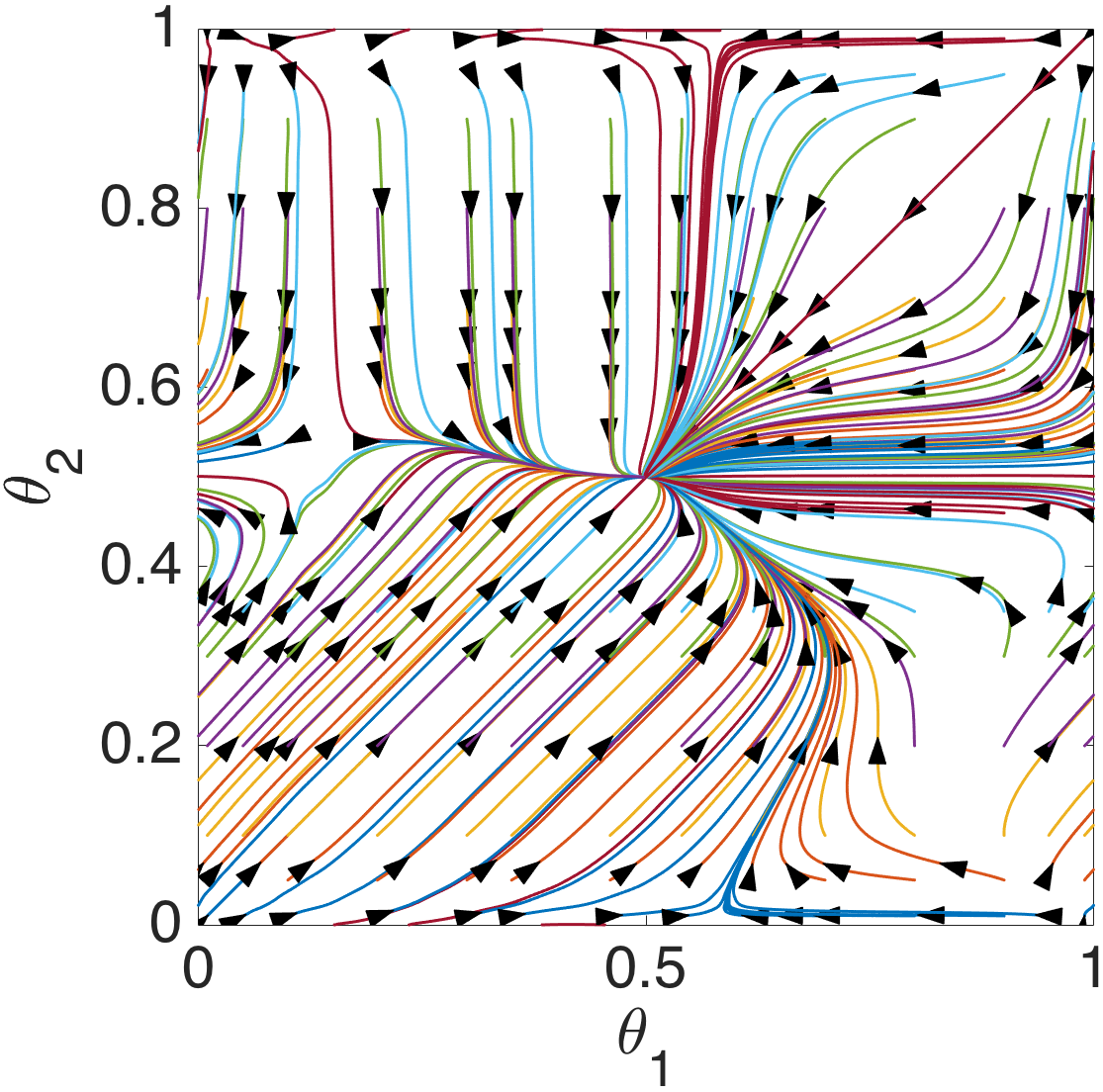
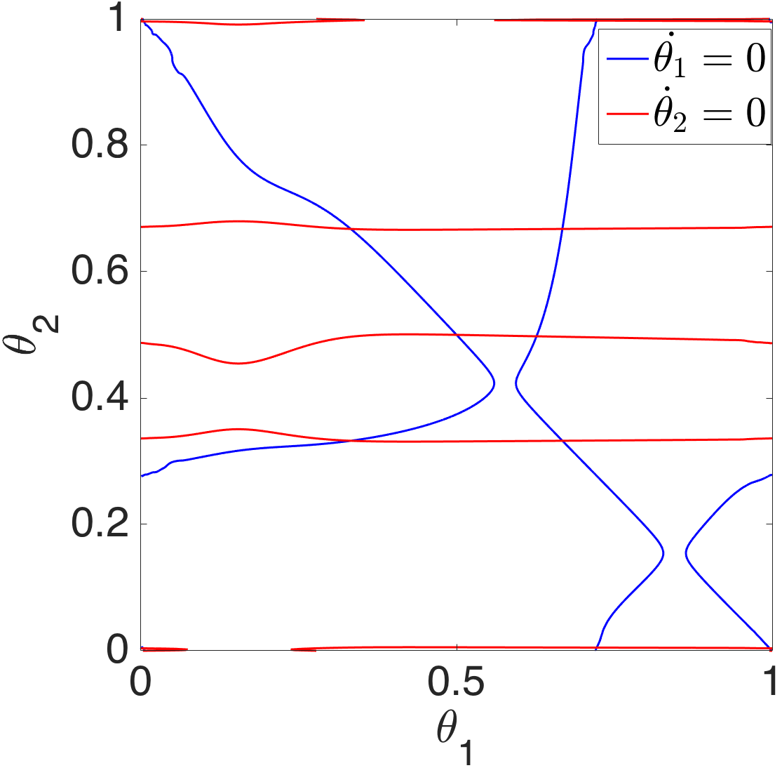
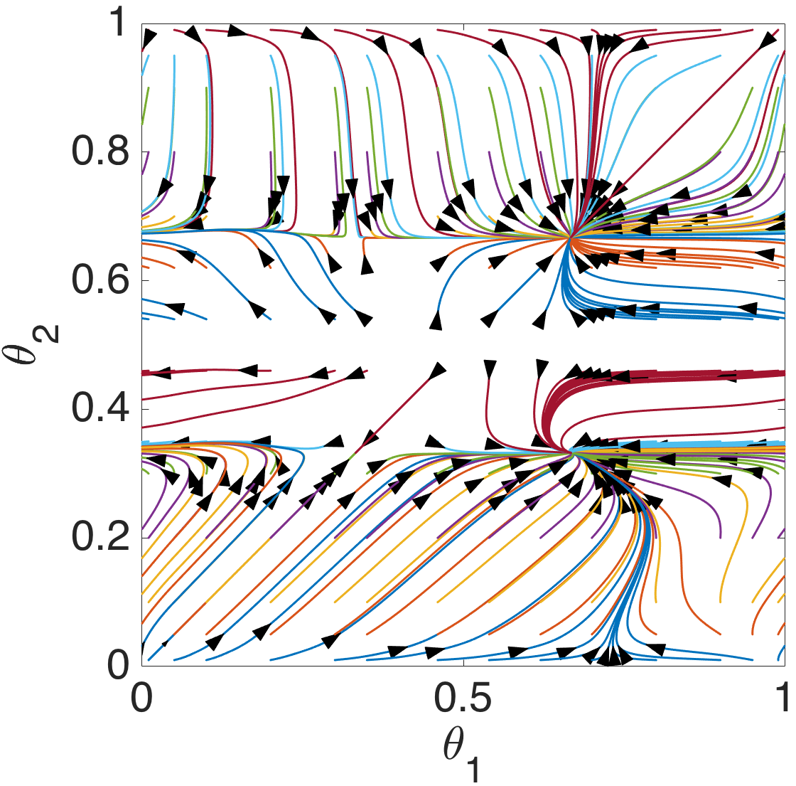
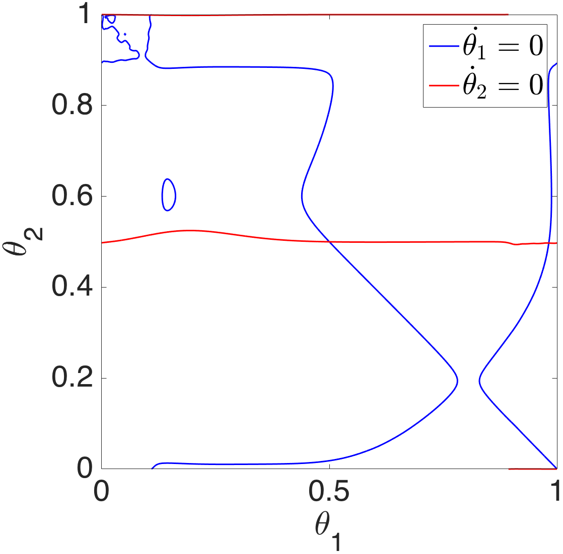
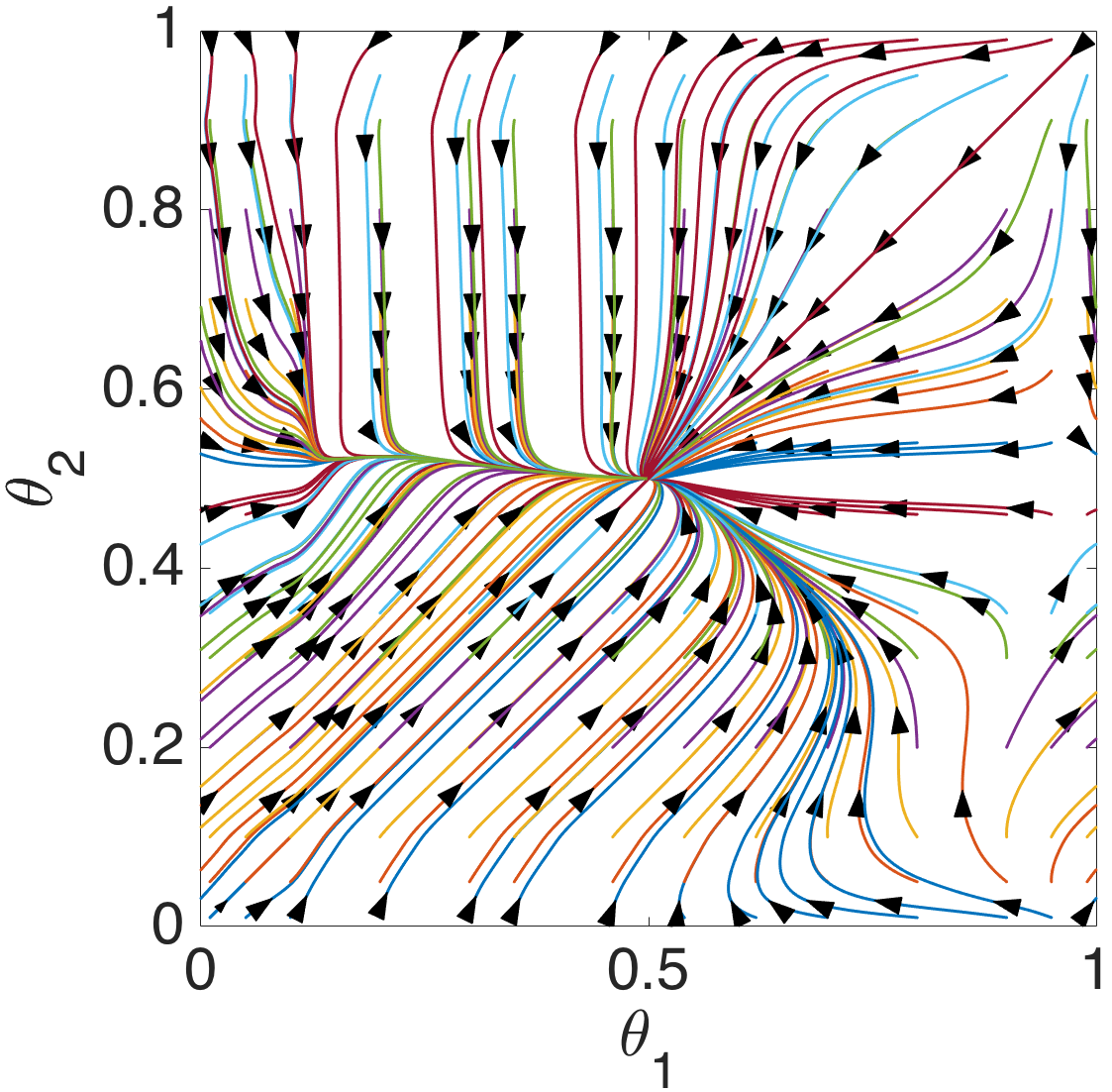
Figure 17: Nullclines and phase planes of Equations (37) when $\alpha\approx 0.032<{\alpha}_{min}$. First row: $\delta=0.0097$ (left) and $\delta=0.03$ (right). Second row: $I_{ext}=35.65$ (left) and $I_{ext}=37.1$ (right). Reflection symmetry is clearly broken.

In this section, using the coupling functions $H_{BN}$ that we computed numerically and with appropriate conditions on coupling strengths ${c}_{i}$, we saw that the phase difference equations admit 10 fixed points when the speed parameter is small (Figures 14-15 (left)), and 4 fixed points when the speed parameter is high (Figures 14-15 (right)). We saw how 4 fixed points (located on the corners of a square) together with 2 saddle points (near the corners of the square), merged to one fixed point (located on the center of the square). We would like to show that in fact 7 fixed points merge and one fixed point bifurcates. To this end, in Section 6.1, we approximate the coupling function $H_{BN}$ by a low order Fourier series.

6 A class of coupling functions producing gait transitions

In this section, we first characterize a class of functions satisfying Assumption 1 and then provide an example based on the bursting neuron model.

Proposition 9.

Let $H(\theta;{\xi})$ be $C^{2}$ and $T$-periodic on $\theta\in[0,T]$ and $C^{1}$ on ${\xi}\in[{\xi}_{1},{\xi}_{2}]$ and let $G(\theta;{\xi})=H(\theta;{\xi})-H(-\theta;{\xi})$. Assume that

(1)

$\exists\,\bar{\xi}\in[{\xi}_{1},{\xi}_{2})$ such that $G(T/3;\bar{\xi})=0$;

(2)

$\forall\,{\xi}>\bar{\xi}$ and $T/3\leq\theta<T/2,\displaystyle\frac{dG}{d{\xi}}(\theta;{\xi})<0$;

(3)

$\exists\,{\xi}_{*}\in(\bar{\xi},{\xi}_{1}]$ such that $\forall\,\theta\in(T/3,T/2)$, and $\bar{\xi}<{\xi}<{\xi}_{*}$, $\displaystyle\frac{d^{2}G}{d\theta^{2}}(\theta;{\xi})=G^{\prime\prime}(\theta;{\xi})<0$.

Then, $\forall\,{\xi}\in(\bar{\xi},{\xi}_{*}),\,G(\theta;{\xi})$ has a unique solution in $[T/3,T/2]$ denoted by $\hat{\theta}({\xi})$ such that $\hat{\theta}(\bar{\xi})=T/3$, $\hat{\theta}({\xi}_{*})=T/2$ and $\hat{\theta}({\xi})$ is a continuous and increasing function on $[\bar{\xi},{\xi}_{*}]$.

Moreover, Equations (24), with the balance equation (26) and ${\eta}({\xi})=\hat{\theta}({\xi})-T/3$, admit a fixed point at $(T-\hat{\theta}({\xi}),\hat{\theta}({\xi}))=(2T/3-{\eta},T/3+{\eta})$, which corresponds to a forward tetrapod gait at ${\xi}=\bar{\xi}$, a tripod gait at ${\xi}={\xi}_{*}$, and a transition gait for ${\xi}\in(\bar{\xi},{\xi}_{*})$.

Proof.

Since $H$ is $T$-periodic, $G(T/2;{\xi})=0,\forall\,{\xi}$, and because $G^{\prime\prime}(\theta;{\xi})<0$ for $\theta\in(T/3,T/2)$ and $\forall\,{\xi}<{\xi}_{*}$,

$$G(T^{-}/2;{\xi})>0\;\;\mbox{where $\;T^{-}/2<T/2\;$ is sufficiently close to $T/2$}.$$ (39)

Also, since $G(T/3;\bar{\xi})=0$ and $\frac{dG}{d{\xi}}(T/3;{\xi})<0$,

$$G(T/3;{\xi})<0,\quad\forall\,{\xi}>\bar{\xi}.$$ (40)

Equations (39) and (40) and Bolzano’s intermediate value theorem imply that for any ${\xi}\in(\bar{\xi},{\xi}_{*})$, $G(\theta;{\xi})$ has a zero $\hat{\theta}({\xi})\in(T/3,T/2)$. $G^{\prime\prime}(\theta;{\xi})<0$ for $\theta\in(T/3,T/2)$ guarantees uniqueness of $\hat{\theta}({\xi})$.

Next we show that $\hat{\theta}({\xi})$ is increasing; i.e., for any $x_{2}>x_{1}\Rightarrow\hat{\theta}(x_{2})>\hat{\theta}(x_{1})$. Fix $x_{1}>\bar{\xi}$. By definition of $\hat{\theta}({\xi})$, $G(\hat{\theta}(x_{1});x_{1})=0$, and because $\frac{dG}{d{\xi}}(\hat{\theta}(x_{1});{\xi})<0,\;\,\forall\,{\xi}>x_{1}$,

$$G(\hat{\theta}(x_{1});x_{2})<0.$$ (41)

Equations (39) and (41) and Bolzano’s theorem imply that $G(\theta;x_{2})$ has a zero in $(\hat{\theta}(x_{1}),T/2)$. Since the zero is unique, it lies at $\hat{\theta}(x_{2})$ and so $\hat{\theta}(x_{2})>\hat{\theta}(x_{1})$. Moreover, $\hat{\theta}(x)$ is continuous: $\forall\,\epsilon>0,\exists\,\delta>0$ such that

$$|x_{1}-x_{2}|<\delta\,\Rightarrow\,|\hat{\theta}(x_{1})-\hat{\theta}(x_{2})|<\epsilon.$$ (42)

We now prove inequality (42). Fix $x_{1}\in(\bar{\xi},{\xi}_{*})$ and choose $\bar{{\xi}}<x_{1}$ small enough such that

$$0<b:=G\left(\hat{\theta}(\bar{{\xi}})+\frac{\epsilon}{2};x_{1}\right)<a:=G\left(\hat{\theta}(\bar{{\xi}})+\frac{\epsilon}{2};\bar{{\xi}}\right).$$

Now $G(\theta;{\xi})$ is continuous, decreasing with ${\xi}$, and $\bar{{\xi}}<x_{1}$, therefore $G(\hat{\theta}(\bar{{\xi}});x_{1})<0$. Since $G(\hat{\theta}({\xi})+{\epsilon}/{2};x_{1})>0$ and $G(\hat{\theta}(\bar{{\xi}});x_{1})<0$ we find that $\hat{\theta}(x_{1})\in(\hat{\theta}(\bar{{\xi}}),\hat{\theta}(\bar{{\xi}})+\epsilon/2)$, and hence that

$$|\hat{\theta}(\bar{{\xi}})-\hat{\theta}(x_{1})|<\frac{\epsilon}{2}.$$ (43)

Since $G(\theta,{\xi})$ is continuous on ${\xi}$, for $\epsilon_{1}=(a-b)/4>0,\,\exists\,\delta_{1}<(x_{1}-\bar{{\xi}})/2$ such that $|x_{2}-x_{1}|<\delta_{1}$ implies that

$$\left|G\left(\hat{\theta}(\bar{{\xi}})+\frac{\epsilon}{2};x_{2}\right)-G\left(\hat{\theta}(\bar{{\xi}})+\frac{\epsilon}{2};x_{1})\right)\right|<\epsilon_{1},$$

and this in turn implies that $G(\hat{\theta}(\bar{{\xi}})+{\epsilon}/{2};x_{2})>0$. Since $\delta_{1}<(x_{1}-\bar{{\xi}})/2$, $x_{2}>\bar{{\xi}}$ and so $G(\hat{\theta}(\bar{{\xi}});x_{2})<0$. Therefore if $\hat{\theta}(x_{2})\in(\hat{\theta}(\bar{{\xi}}),\hat{\theta}(\bar{{\xi}})+\epsilon/2)$ then

$$|\hat{\theta}(x_{2})-\hat{\theta}(\bar{{\xi}})|<\frac{\epsilon}{2}.$$ (44)

Finally, Equations (43) and (44) imply that for $\delta=\delta_{1}$, if $|x_{1}-x_{2}|<\delta$ then $|\hat{\theta}(x_{1})-\hat{\theta}(x_{2})|<\epsilon$. ∎

As an example, we next show that $H_{app}(\theta;{\xi})$, an explicit function which approximates $H_{BN}(\theta;{\xi})$, satisfies assumptions (1), (2) and (3) in Proposition 9.

6.1 Example of an explicit coupling function

In this section, we approximate $H_{app}$ by its Fourier series and derive an explicit function $H_{app}$ as follows. To derive $H_{app}$, we first computed the coefficients of the Fourier series of $H_{BN}$, and then, using polyfit in Matlab, fitted an appropriate quadratic function for each coefficient, obtaining

Figure 18: Fourier coefficients of $H_{app}$

$$a_{0}(\delta) =-80.8384\delta^{2}+2.6862\delta-0.0986,$$ (45a)

$$a_{1}(\delta) =-137.9839\delta^{2}+7.5308\delta-0.1433,$$ (45b)

$$b_{1}(\delta) =77.9417\delta^{2}-3.9694\delta-0.0720,$$ (45c)

$$a_{2}(\delta) =-184.2374\delta^{2}+8.9996\delta-0.0420,$$ (45d)

$$b_{2}(\delta) =68.0350\delta^{2}+0.6692\delta-0.1077.$$ (45e)

By definition, $H_{{app}}(\theta;\delta)$ on $[0\;1]\times[0.008\;0.024]$ is

$$H_{{app}}(\theta;\delta)\;:=\;\displaystyle\sum_{k=0}^{2}a_{k}(\delta)\cos(2\pi k\theta)+\displaystyle\sum_{k=1}^{2}b_{k}(\delta)\sin(2\pi k\theta).$$

In Figure 19, we compare the approximate coupling function $H_{app}$ with $H_{BN}$ for the values of $\delta$ at the endpoints of the interval of interest.

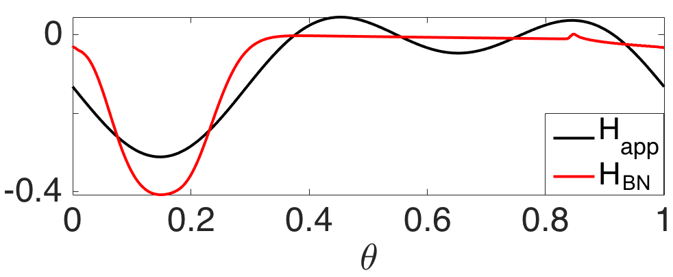
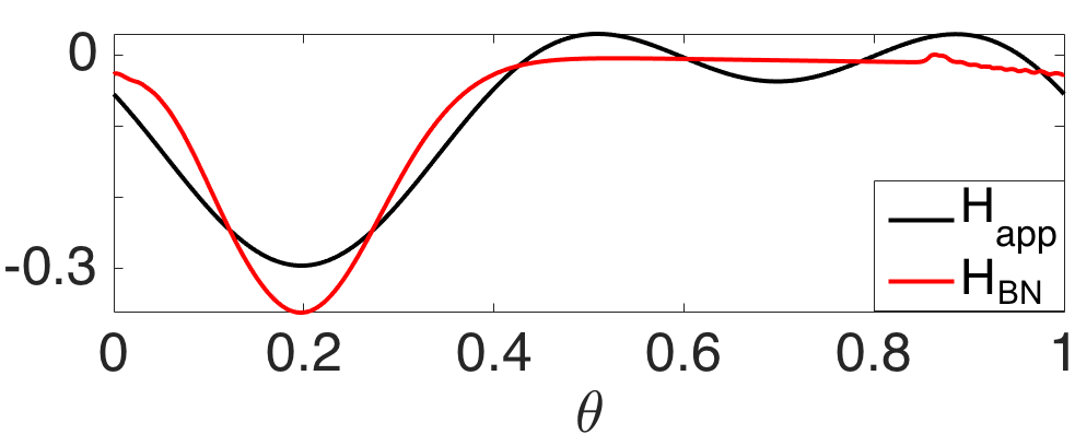
Figure 19: The coupling function $H_{BN}$ and its approximation $H_{app}$ are shown for $\delta=0.01$ (left) and $\delta=0.024$ (right).

We next verify that

$$G_{app}(\theta;\delta):=H_{app}(\theta;\delta)-H_{app}(-\theta;\delta)=2b_{1}(\delta)\sin(2\pi\theta)+2b_{2}(\delta)\sin(4\pi\theta),$$ (46)

satisfies conditions (1), (2), and (3) of Proposition 9.

Conditions of Proposition 9

Figure 20 shows the graphs of $G_{app}$ for different values of $\delta$. Since we are only interested in the interval $[1/3,1/2]$, we only show the $G_{app}$’s in this interval.

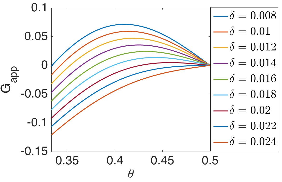
Figure 20: The graphs of $G_{app}$ on $[1/3,1/2]$ and for different values of $\delta$ are shown.

As Figure 20 shows, for $\bar{\delta}=0.008$, $G_{app}$ equals to zero at $1/3$: $G_{app}(1/3;0.008)=0$. In the interval $[1/3,1/2]$, as $\delta$ increases, at each point $\theta$, $G_{app}$ decreases: $dG_{app}/d\delta<0$. For $\delta<\delta_{*}=0.0218$, the graph of $G_{app}$ is concave down: $G^{\prime\prime}_{app}<0$. One can compute the zero of $G_{app}(1/3;\delta)$, $dG_{app}/d\delta$, and $G^{\prime\prime}_{app}$ explicitly and verify the above conditions.

Computing ${\eta}$. We show that

$${\eta}(\delta)=\frac{1}{2\pi}\arccos\left(\frac{-b_{1}(\delta)}{2b_{2}(\delta)}\right)-\frac{1}{3},$$ (47)

is a unique non-constant and non-decreasing solution of $H_{app}\left({2}/{3}-{\eta};\delta\right)=H_{app}\left({1}/{3}+{\eta},\delta\right)$. Note that ${\eta}$ is defined only where $\left|{-b_{1}(\delta)}/{2b_{2}(\delta)}\right|\leq 1$. Figure 21 (left) shows that $\exists\delta_{*}\approx 0.0218$ such that for $\delta\in[0.008,\delta_{*}]$, $-1\leq{-b_{1}(\delta)}/{2b_{2}(\delta)}<0$. Therefore, we let $[0.008,\delta_{*}]$ be the domain of ${\eta}$, where $\delta_{*}$ satisfies

$$\frac{-b_{1}(\delta_{*})}{2b_{2}(\delta_{*})}=-1.$$ (48)

Figure 21 (right) shows the graph of ${\eta}$. Note that the range of ${\eta}$ is approximately $[0,1/6]$, as desired.

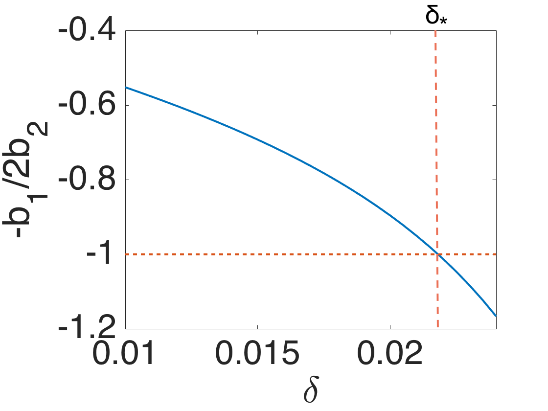
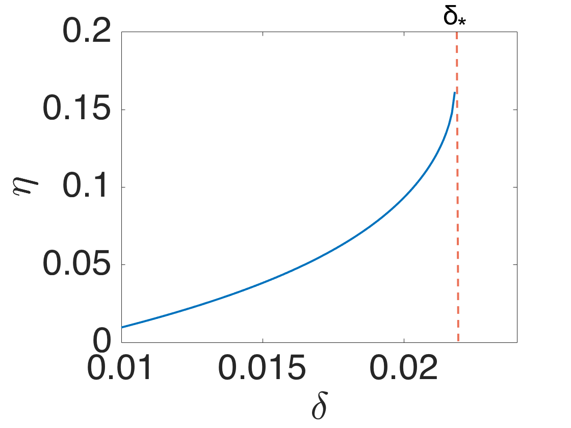
Figure 21: (Left) the graph of ${-b_{1}(\delta)}/{2b_{2}(\delta)}$ which determines the domain of ${\eta}$ defined in Equations (47); (right) the graph of ${\eta}$.

A simple calculation shows that because $\cos(2\pi-x)=\cos x$,

$$\cos\left(2\pi k\left({2}/{3}-{\eta}\right)\right)=\cos\left(2\pi k-\left(2\pi k\left({2}/{3}-{\eta}\right)\right)\right)=\cos\left(2\pi k\left({1}/{3}+{\eta}\right)\right),$$

and therefore the cosine terms in the Fourier series cancel, resulting in

$$H_{app}\left(\frac{2}{3}-{\eta};\delta\right)=H_{app}\left(\frac{1}{3}+{\eta};\delta\right) \Longleftrightarrow$$ (49)

$$\sum_{k=1}^{2}b_{k}(\delta)\sin\left(2\pi k\left({2}/{3}-{\eta}\right)\right) =\sum_{k=1}^{2}b_{k}(\delta)\sin\left(2\pi k\left({1}/{3}+{\eta}\right)\right).$$

Using the fact that $\sin(2\pi-x)=-\sin x$, we have

$$\sin\left(2\pi k\left({2}/{3}-{\eta}\right)\right)=-\sin\left(2\pi k-\left(2\pi k\left({2}/{3}-{\eta}\right)\right)\right)=-\sin\left(2\pi k\left({1}/{3}+{\eta}\right)\right),$$

and so the right hand equality of Equation (49) can be written as follows.

$$\quad\quad\sum_{k=1}^{2}b_{k}(\delta)\sin\left(2\pi k\left({2}/{3}-{\eta}\right)\right)=\sum_{k=1}^{2}b_{k}(\delta)\sin\left(2\pi k\left({1}/{3}+{\eta}\right)\right)$$ (50a)

$$\Longleftrightarrow \quad-\sum_{k=1}^{2}b_{k}(\delta)\sin\left(2\pi k\left({1}/{3}+{\eta}\right)\right)=\sum_{k=1}^{2}b_{k}(\delta)\sin\left(2\pi k\left({1}/{3}+{\eta}\right)\right)$$ (50b)

$$\Longleftrightarrow \quad b_{1}(\delta)\sin\left(2\pi\left({1}/{3}+{\eta}\right)\right)+b_{2}(\delta)\sin\left(4\pi\left({1}/{3}+{\eta}\right)\right)=0.$$ (50c)

Now using the double-angle identity, $\sin(2x)=2\sin x\cos x$, we get

$$H_{app}\left(\frac{2}{3}-{\eta};\delta\right)=H_{app}\left(\frac{1}{3}+{\eta};\delta\right)\Longleftrightarrow\sin\left(2\pi(1/3+{\eta})\right)\left[b_{1}(\delta)+2b_{2}(\delta)\cos\left(2\pi(1/3+{\eta})\right)\right]=0.$$

Since we are looking for a non-constant and non-decreasing solution, we solve

$$b_{1}(\delta)+2b_{2}(\delta)\cos\left(2\pi(1/3+{\eta})\right)=0,$$

for ${\eta}$, which gives ${\eta}$ as in Equation (47).

Therefore, by Proposition 9, Equations (24), with $H=H_{app}$ and the balance equation (26) admit a fixed point at $(T-\hat{\theta}({\xi}),\hat{\theta}({\xi}))=(2T/3-{\eta},T/3+{\eta})$, which corresponds to a forward tetrapod gait at ${\xi}=\bar{\xi}$, a tripod gait ${\xi}={\xi}_{*}$, and a transition gait for ${\xi}\in(\bar{\xi},{\xi}_{*})$.

In what follows we assume Equations (37) with $H=H_{app}$. We compute $H_{app}^{\prime}$, and show that it satisfies conditions of Propositions 3, 4, and 5.

$$H_{app}^{\prime}=-2\pi\displaystyle\sum_{k=1}^{2}k\;a_{k}(\delta)\sin(2\pi k\theta)+2\pi\displaystyle\sum_{k=1}^{2}k\;b_{k}(\delta)\cos(2\pi k\theta).$$ (51)

Conditions of Proposition 3

First, we verify the stability of $(2/3-{\eta},1/3+{\eta})$.

$$H_{app}^{\prime}\left({1}/{3}+\eta,\delta\right)\pm H_{app}^{\prime}\left({2}/{3}-\eta,\delta\right)>0,\quad\forall\delta\in[0.01,\delta_{*}].$$

Substituting Equation (47) in the derivative of $H_{app}$, Equation (51), and using trigonometrical identities yields

$$H_{app}^{\prime}\left(\frac{1}{3}+{\eta};\delta\right)+H_{app}^{\prime}\left(\frac{2}{3}-{\eta};\delta\right)=-2\pi\;\displaystyle\frac{4b_{2}^{2}(\delta)-b_{1}^{2}(\delta)}{b_{2}(\delta)}>0,$$

and

$$H_{app}^{\prime}\left(\frac{1}{3}-{\eta};\delta\right)+H_{app}^{\prime}\left(\frac{2}{3}-{\eta};\delta\right)=\pi\left(a_{1}(\delta)-2\frac{a_{2}(\delta)b_{1}(\delta)}{b_{2}(\delta)}\right)\;\displaystyle\frac{\sqrt{4b_{2}^{2}(\delta)-b_{1}^{2}(\delta)}}{b_{2}(\delta)}>0,$$

which are positive because $4b_{2}^{2}(\delta)-b_{1}^{2}(\delta)>0$ on $[0.008,\delta_{*}]$, $a_{1}(\delta),b_{1}(\delta),b_{2}(\delta)<0$, and $a_{2}(\delta)>0$ (see Figures 21(left) and 18). Therefore, by Proposition 4, for ${\alpha}<{\alpha}_{max}$ (resp. ${\alpha}>{\alpha}_{max}$), $(2/3-{\eta},1/3+{\eta})$ is a sink (resp. saddle point).

Conditions of Proposition 4

Next, we verify the stability of $(1/3+{\eta},1/3+{\eta})$, $(1/3+{\eta},2/3-{\eta})$, and $(2/3-{\eta},2/3-{\eta})$.

$H_{app}^{\prime}\left({2}/{3}-\eta,\delta\right)$ changes sign, on the domain of ${\eta}$, i.e., $[0.01,\delta_{*}]$. Substituting Equation (47) in the derivative of $H_{app}$, Equation (51), and using trigonometrical identities yields

$$H_{app}^{\prime}\left(\frac{2}{3}-{\eta};\delta\right)=-\displaystyle\frac{\pi}{b_{2}(\delta)}\sqrt{4b_{2}^{2}(\delta)-b_{1}^{2}(\delta)}\left(a_{1}(\delta)-2\frac{a_{2}(\delta)b_{1}(\delta)}{b_{2}(\delta)}+\sqrt{4b_{2}^{2}(\delta)-b_{1}^{2}(\delta)}\right).$$

Figure 22 (left) shows that $H_{app}^{\prime}\left({2}/{3}-{\eta};\delta\right)$ changes sign from positive to negative on $\delta\in[0.01,\delta_{*}]$, at some $\delta$ near $0.01$. We will see that through a transcritical bifurcation, $(1/3+{\eta},1/3+{\eta})$ becomes a saddle point from a sink. The reason is that by Proposition 4, as $H^{\prime}_{app}(2/3-{\eta};\delta)$ changes sign, one of the eigenvalues of $(1/3+{\eta},1/3+{\eta})$ becomes positive while the other one remains negative. For ${\alpha}>{\alpha}_{min}$, the fixed points $(1/3+{\eta},2/3-{\eta})$ and $(2/3-{\eta},2/3-{\eta})$ are always sinks.

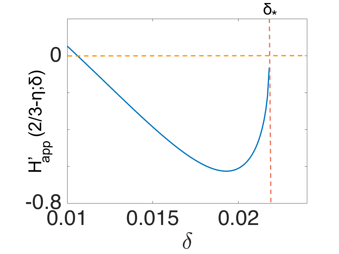
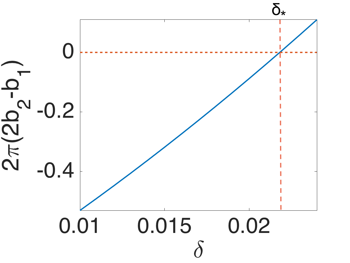
Figure 22: (Left) $H_{app}^{\prime}\left(\frac{2}{3}-\eta;\delta\right)<0$, (right) $H^{\prime}_{app}\left(\frac{1}{2};\delta\right)$.

Conditions of Proposition 5

Finally, we verify the stability types of $(1/2,1/2)$ and $(0,0)$.

• For $\delta<\delta_{*}$, $H_{app}^{\prime}\left({1}/{2};\delta\right)<0$, while for $\delta>\delta_{*}$, $H_{app}^{\prime}\left({1}/{2};\delta\right)>0$. Setting $\theta=1/2$ in Equation (51), we get

  $$H_{app}^{\prime}(1/2;\delta)=2\pi(2b_{2}(\delta)-b_{1}(\delta)).$$

  By the definition of $\delta_{*}$, for $\delta<\delta_{*}$, $-b_{1}/2b_{2}<-1$. Figure 22 (right) shows that $H_{app}^{\prime}(1/2,\delta)$ changes sign from negative to positive at $\delta=\delta_{*}$. This guarantees that the fixed point $(1/2,1/2)$ becomes stable as $\delta$ passes $\delta_{*}$.

• $H_{app}^{\prime}(0;\delta)<0$. Setting $\theta=0$ in Equation (51), we obtain $H_{app}^{\prime}(0;\delta)=2\pi(b_{1}(\delta)+2b_{2}(\delta))$, which is negative because for $\delta\in[0.0080.024]$ both $b_{1}(\delta)$ and $b_{2}(\delta)$ are negative (see Figure 18). This guarantees that $(0,0)$ is always a source.

6.2 Bifurcation diagrams: balance conditions and equal contralateral couplings

In this section, we consider Equations (37) for $H=H_{app}$ and study the bifurcations as $\delta$ increases. We draw the bifurcation diagrams (Figure 24) using Matcont, a Matlab numerical continuation packages for the interactive bifurcation analysis of dynamical systems [23]. We first consider the system with ${\alpha}=1/3$. When $\delta$ is small, $\delta=0.01$, as Figures 23 (first row, left) shows, there exist 12 fixed points: 6 saddle points, 2 sources, and 4 sinks. In this case, $(1/3+{\eta},1/3+{\eta})$ is a sink (shown by a green dot in Figure 23). As $\delta$ increases and reaches $\delta^{(0)}$ (Figure 24 (left)), through a transcritical bifurcation, $(1/3+{\eta},1/3+{\eta})$ becomes a saddle. Further, as $\delta$ reaches $\delta^{(1)}$, through a saddle node bifurcation, a sink (green dot) and a saddle (orange star) annihilate each other and 10 fixed points remain: 5 saddle points, 2 sources, and 3 sinks (see Figures 23 (first row, right) and 24 (left)). Note that the two extra fixed points were not observed in the case of the numerically computed $H$ and the transcritical and saddle node bifurcations did not occur.

As $\delta$ increases further to $\delta^{(2)}$, through a degenerate bifurcation, 4 fixed points disappear and only 6 fixed points remain (see Figures 23 (second row, left) and 24 (left)).

When $\delta$ reaches $\delta^{(3)}$, 2 fixed points vanish in a saddle node bifurcation and 4 fixed points remain: 2 saddle points, a source, and a sink (see Figures 23 (second row, right) and 24 (left)). Note that 2 saddle points and 1 source near the edges of the square remain unchanged while $\delta$ varies. Figure 24 (left) shows the bifurcation diagram when $\alpha=1/3$.

Remark 4.

Figure 24 (right) shows the bifurcation diagram when $\alpha=1/2$. In this case, due to reflection symmetry about $\theta^{(1)}=\theta^{(2)}$, there is no saddle node bifurcation at $\delta=\delta^{(3)}$ (as in the case of ${\alpha}=1/3$), and 7 fixed points merge to $(1/2,1/2)$ in a very degenerate bifurcation.

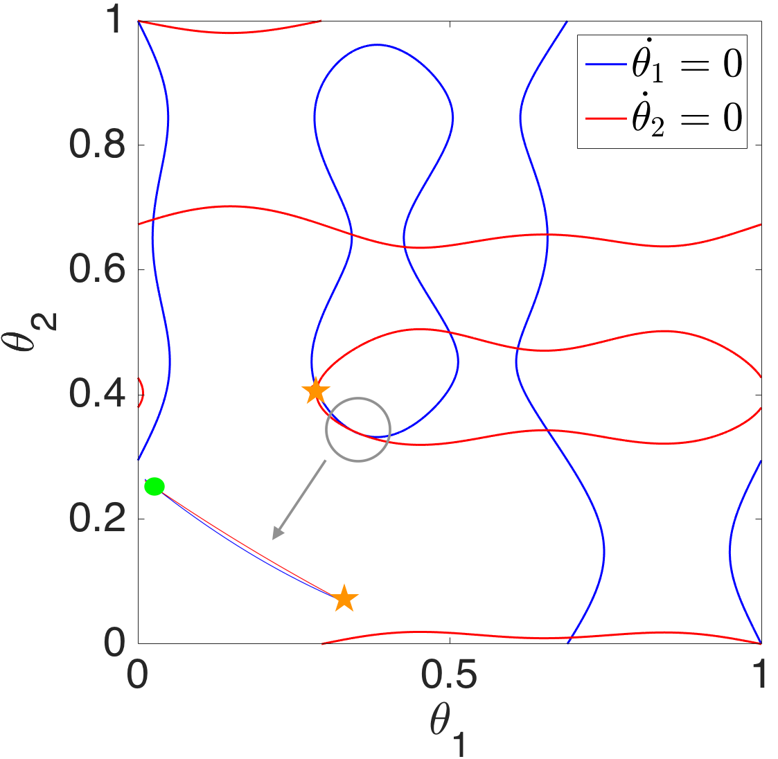
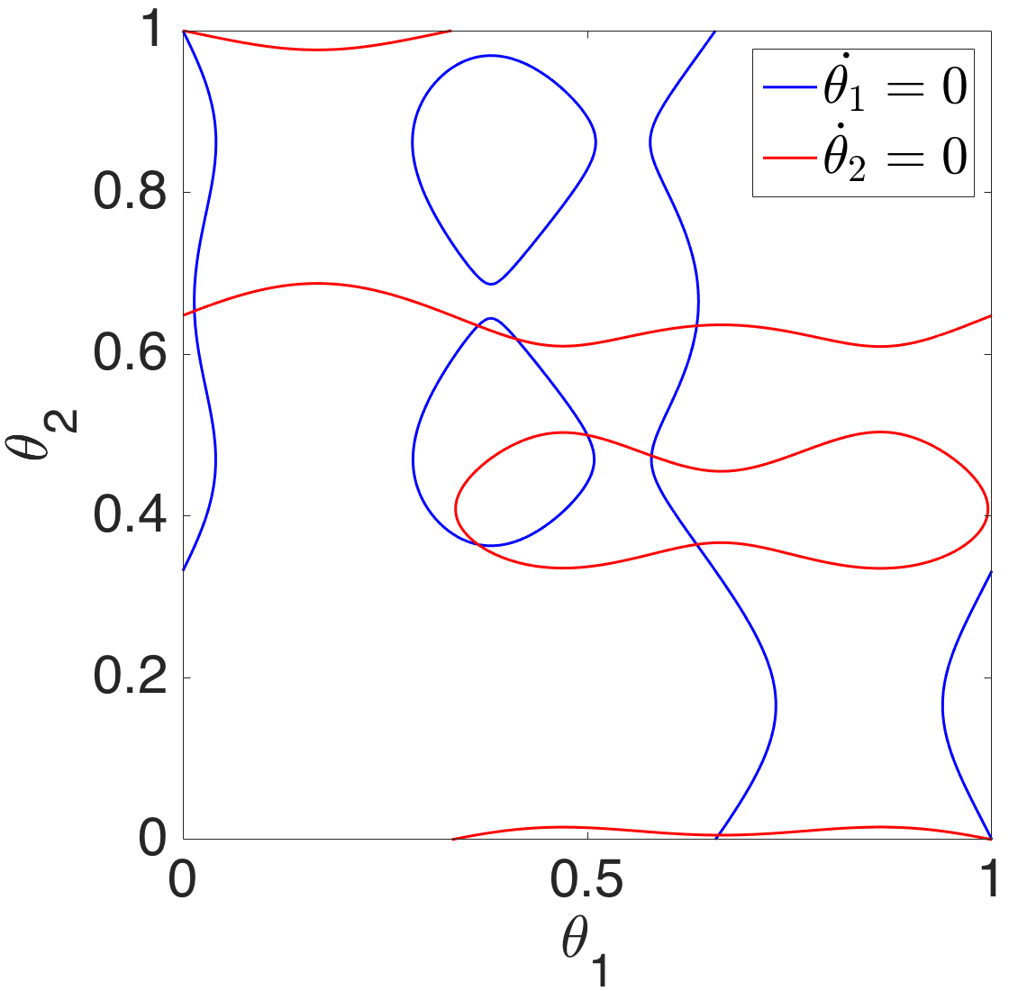
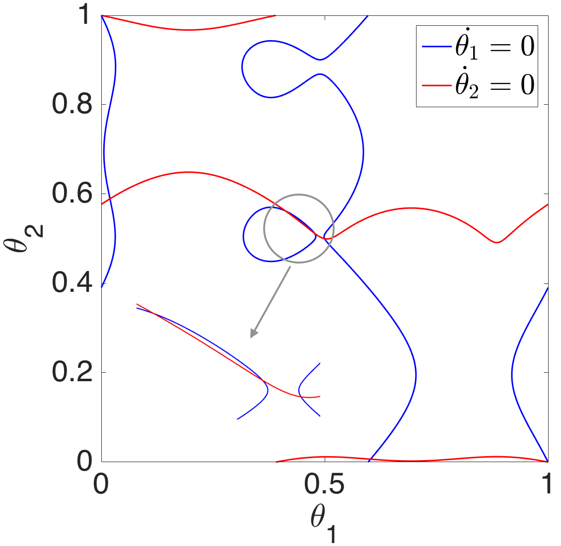
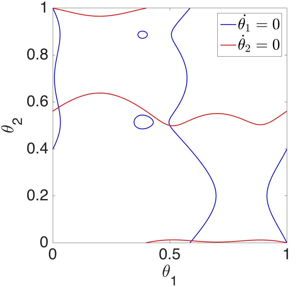
Figure 23: Nullclines of Equations (37) with $H=H_{app}$, ${\alpha}=1/3$ and 4 values of $\delta$ are shown. Note enlargements of nullcline intersections in left column. First row: $\delta=0.01$ (left), $\delta=0.014$ (right); as $\delta$ increases, a transcritical bifurcation at $\delta=\delta^{(0)}>0.01$ and a saddle node bifurcation at $\delta=\delta^{(1)}<0.014$ occur. Second row: $\delta=0.023$ (left), $\delta=0.025$ (right); as $\delta$ increases, a degenerate bifurcation at $\delta=\delta^{(2)}>0.023$ and a saddle node bifurcation at $\delta=\delta^{(3)}>0.025$ occur. The corresponding bifurcation diagram is shown in Figure 24 (left)). Note that the green dot indicates a sink and the orange star indicates a saddle point. See text for further explanation.

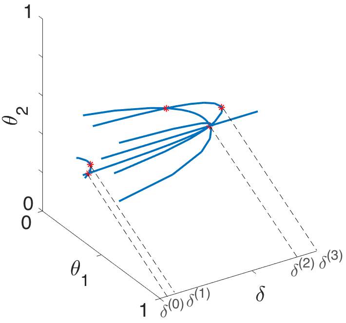
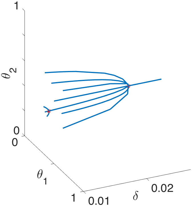
Figure 24: Partial bifurcation diagrams of Equations (37) with $H=H_{app}$ for ${\alpha}=1/3$ (left) and ${\alpha}=1/2$ (right). In both cases the coupling strengths are balanced, but the ${\alpha}=1/3$ case is not rostrocaudally symmetric. The source $(0,0)$ and two saddle points near $\theta_{1}=0$ and $\theta_{2}=0$ are omitted.

7 Gaits deduced from fruit fly data fitting

In this section, we use two sets of coupling strengths which were estimated for slow, medium, and fast wild-type fruit flies in our reduced model on the torus and show the existence of stable tetrapod gaits at low frequency and stable tripod gaits at higher frequency. To vary frequency, we change $I_{ext}$ in the first set of estimates in Section 7.1, and we change $\delta$ in the second set of estimates in Section 7.2. Unlike the gait transitions of Section 4, the fitted data predict different coupling strengths across the speed range. As in previous sections, we display both results from the bursting neuron model and the nullclines and phase planes from the reduction to the $(\theta_{1},\theta_{2})$ plane.

7.1 Dataset 1

We first exhibit a gait transition from tetrapod to tripod as $I_{ext}$ increases.

	$\hat{\omega}$	${c}_{1}$	${c}_{2}$	${c}_{3}$	${c}_{4}$	${c}_{5}$	${c}_{6}$	${c}_{7}$
slow	9.92	0.3614	0.1478	0.1780	0.1837	0.2509	0.3409	0.1495
medium	12.48	0.2225	0.6255	0.4715	0.1436	0.3895	0.7921	0.2964
fast	15.52	0.0580	0.8608	0.6726	0.0470	0.4294	1.1498	0.8500

Table 2: Values of estimated frequency and coupling strengths for slow, medium, and fast wild-type fruit flies.

Table 2 shows the coupling strengths ${c}_{i}$ which were estimated for slow (represented by coupled frequency $\hat{\omega}=9.92$), medium ($\hat{\omega}=12.48$), and fast ($\hat{\omega}=15.52$) wild-type fruit flies. These fits were obtained after linearizing Equations (17) and adding i.i.d. zero mean Gaussian noise to each equation. The touchdown times of every leg are treated as measurements of the phase of its associated oscillator in Equations (17), additionally corrupted by a zero mean Gaussian measurement noise. To incorporate the circular nature of phase measurements, the initial condition distribution for Equations (17) is modeled by a mixture Gaussian distribution. For each sequence of leg touchdowns, a Gaussian sum filter [24] is used to compute the distribution and the log-likelihood of leg touchdown times. The aggregate log-likelihood for pooled sequences of leg touchdowns for different flies is maximized to compute the maximum likelihood estimates (MLEs) of coupling strengths, phase differences, and variance of the i.i.d. measurement noises.

We choose 3 different values of $I_{ext}$: $I_{ext}=35.95$ for slow (represented by uncoupled frequency $\omega=8.76$), $I_{ext}=36.85$ for medium ($\omega=12.64$), and $I_{ext}=37.65$ for fast ($\omega=14.85$) speeds. Note that in general $\hat{\omega}<\omega$, because we assume that all the couplings are inhibitory, ${c}_{i}H<0$, although the coupled frequency corresponding to the slow and fast speed are not less than the uncoupled frequency in our simulations below. Also note that the medium and fast speed coupling parameters (Table 2, second and third rows) are far from balanced.

Figure 25 shows solutions of the 24 ODEs for the following initial conditions:

$$v_{1}=-40,\;v_{2}=10,\;v_{3}=-10,\;v_{4}=30,\;v_{5}=15,\;v_{6}=-30,\;$$ (52)

and for $i=1,\cdots,6$, the $m_{i}$’s, ${w}_{i}$’s, and $s_{i}$’s take their steady state values as in Equation (11). In Figure 25 (left), $I_{ext}=35.95$ and the coupling strengths ${c}_{i}$ are as in Table 2, first row. In Figure 25 (middle), $I_{ext}=36.85$ and the coupling strengths ${c}_{i}$ are as in Table 2, second row. In Figure 25 (right), $I_{ext}=37.65$ and the coupling strengths ${c}_{i}$ are as in Table 2, third row. As we expect, these respectively depict tetrapod, transition, and tripod gaits. We computed the solutions up to time $t=5000$ ms but only show the time windows $[4800,5000],$ after transients have died out.

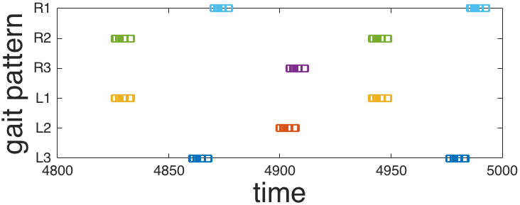
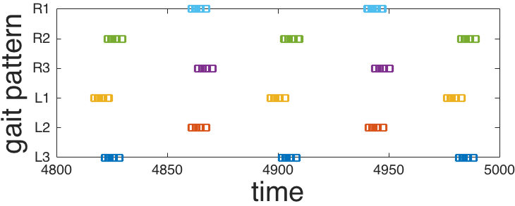
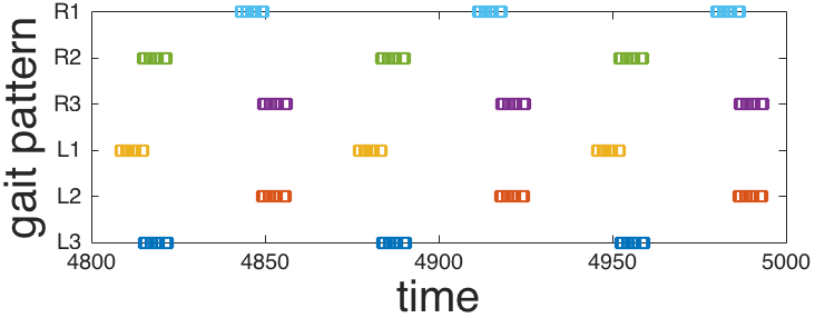
Figure 25: (Left to right) A solution of 24 ODEs for $I_{ext}=35.95$ and ${c}_{i}$’s as in the first row of Table 2; $I_{ext}=36.85$ and ${c}_{i}$’s as in the second row of Table 2; and for $I_{ext}=37.65$ and ${c}_{i}$’s as in the third row of Table 2.

Figure 26 shows the nullclines (first row) and the corresponding phase planes (second row) of Equation (24) for the three different values of $I_{ext}$. As Figure 26 (left) depicts, when the speed parameter is small, there exist 6 fixed points: 2 sinks which correspond to the forward and backward tetrapod gaits, a source, and 3 saddle points. As Figure 26 (middle) depicts, when the speed parameter increases, there exist 4 fixed points: a sink which corresponds to the transition gait, a source, and 2 saddle points. As Figure 26 (right) depicts, when the speed parameter is large, there exist only 2 fixed points: a sink corresponding to the tripod gait and a saddle point.

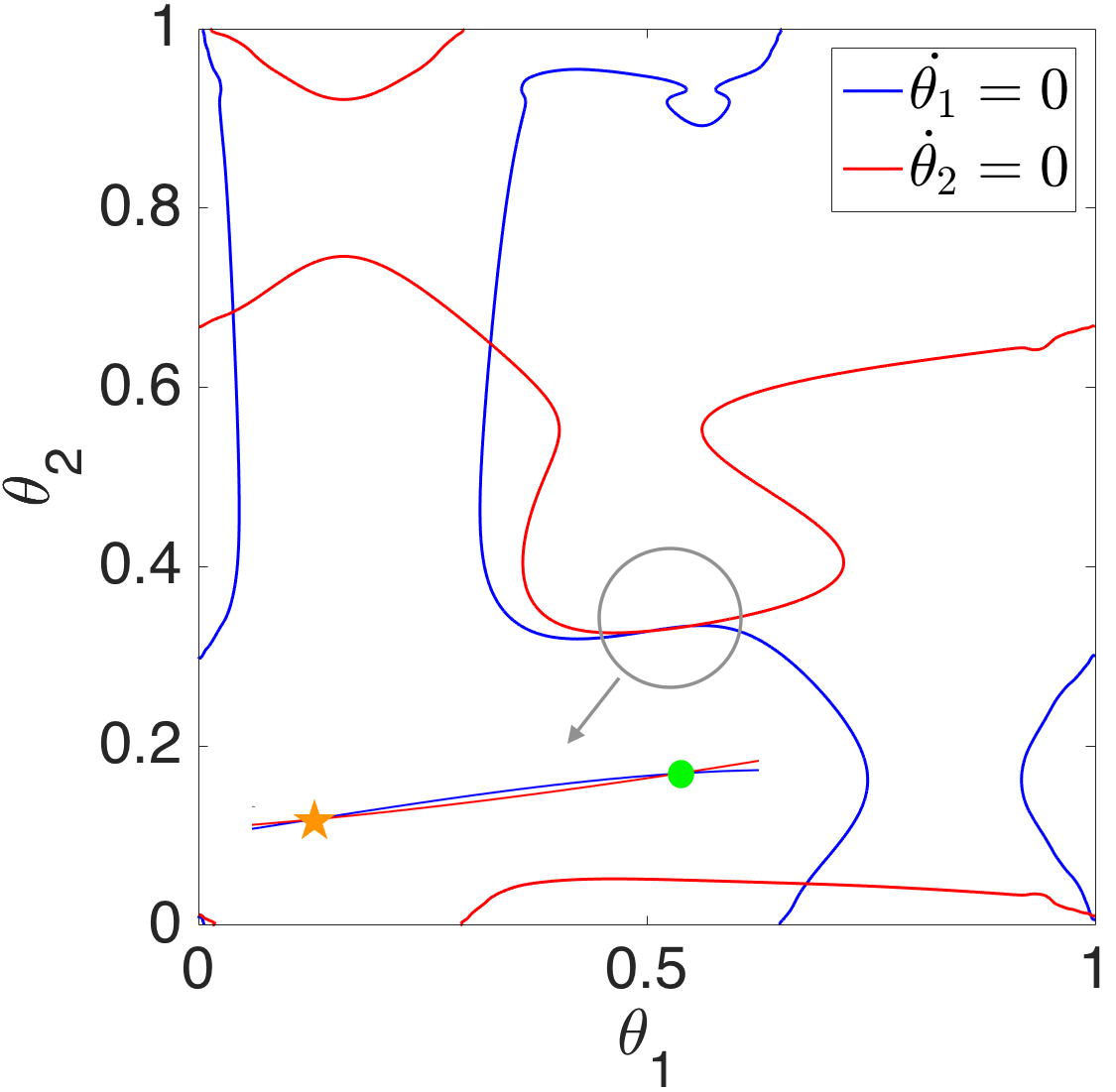
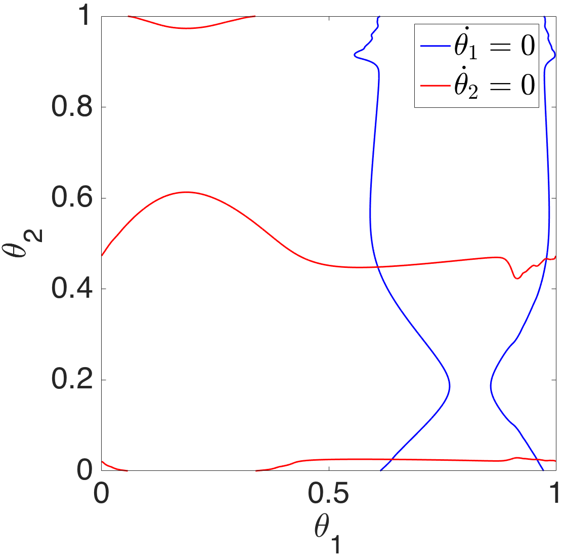
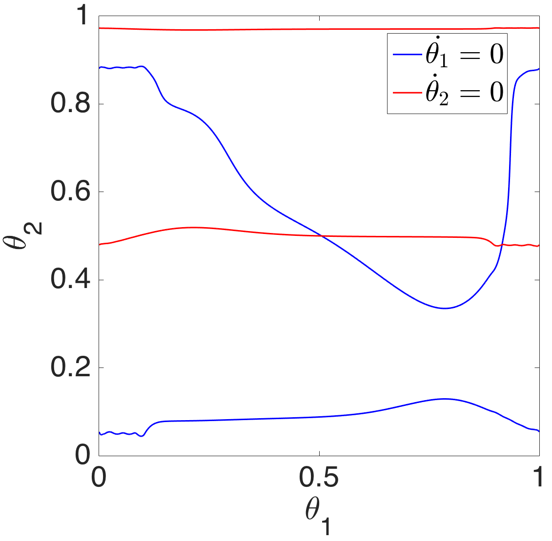
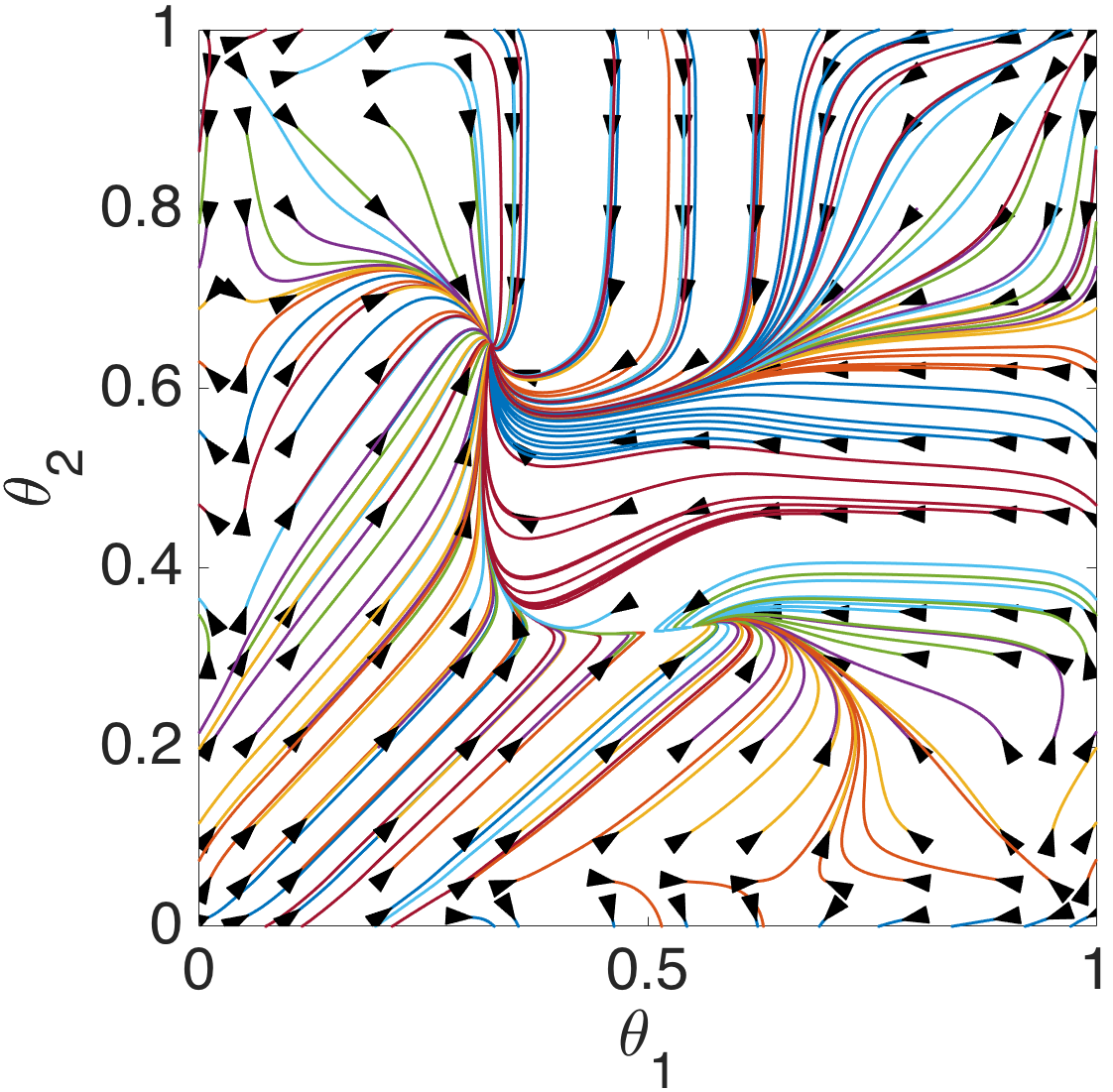
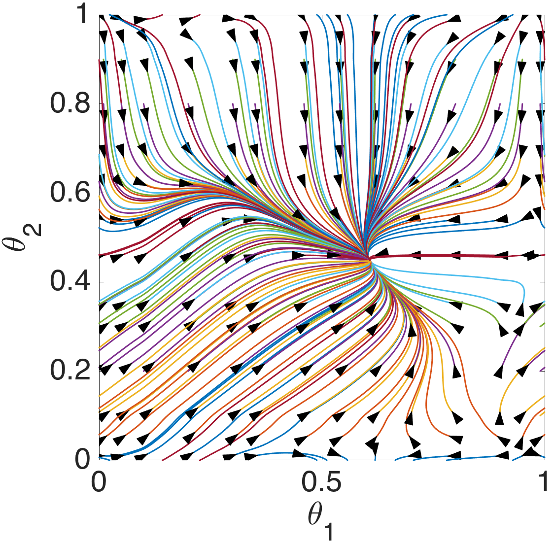
Figure 26: (First row: left to right) Nullclines of Equations (24) for $I_{ext}=35.95$ and ${c}_{i}$’s as in the first row of Table 2; $I_{ext}=36.85$ and ${c}_{i}$’s as in the second row of Table 2; and for $I_{ext}=37.65$ and ${c}_{i}$’s as in the third row of Table 2. (Second row: left to right) Corresponding phase planes. Note that the green dot indicates a sink and the orange star indicates a saddle point. See text for further explanation.

7.2 Dataset 2

In this section, we show a gait transition from tetrapod to tripod, as $\delta$ increases.

	$\hat{\omega}$	${c}_{1}$	${c}_{2}$	${c}_{3}$	${c}_{4}$	${c}_{5}$	${c}_{6}$	${c}_{7}$
medium	12.23	0.2635	1.2860	2.9480	1.3185	1.3885	2.5025	1.2265
fast	15.65	2.9145	2.5610	2.6160	2.9135	5.1800	5.4770	2.6165

Table 3: Values of estimated frequency and coupling strengths for medium, and fast free-walking wild-type fruit flies.

Table 3 shows the coupling strengths ${c}_{i}$ which were estimated for medium (represented by coupled frequency $\hat{\omega}=12.23$) and fast ($\hat{\omega}=15.65$) wild-type fruit flies. These fits are obtained using linearized ODEs similar to Section 7.1. However, to obtain these fits, touchdown sequences for different flies are concatenated to obtain a single large sequence and a Kalman filter is used to compute the distribution and the log-likelihood of leg touchdown times. The MLEs for coupling strengths are obtained by maximizing the aggregate likelihood for the concatenated touchdown sequence.

We choose 2 different values of $\delta$, $\delta=0.014$ for medium (represented by uncoupled frequency $\omega=3.57$), and $\delta=0.03$ for fast ($\omega=6.91$) speeds [22]. As noted earlier in Section 2.1.1, as $\delta$ varies in the bursting neuron model, the range of frequency does not match the range of frequency estimated from data. In spite of this, we show that the estimated coupling strengths in the low speed range (small $\delta$) give a tetrapod gait and in the high speed range (large $\delta$) give a tripod gait.

Figure 27 shows solutions of the 24 ODEs for the following initial conditions.

$$v_{1}=-10,\;v_{2}=-40,\;v_{3}=-30,\;v_{4}=-40,\;v_{5}=5,\;v_{6}=20,\;$$ (53)

and for $i=1,\cdots,6$, $m_{i}$’s, ${w}_{i}$’s, and $s_{i}$’s take their steady state values as in Equation (11). In Figure 27 (left), $\delta=0.014$ and the coupling strengths ${c}_{i}$ are as in Table 3, first row. In Figure 27 (right), $\delta=0.03$ and the coupling strengths ${c}_{i}$ are as in Table 3, second row. As we expect, Figure 27 (left to right) depicts transition (still very close to a tetrapod gait) and tripod gaits, respectively. We computed the solutions up to time $t=5000$ ms but only show the time window $[4000,5000],$ after transients have died out.

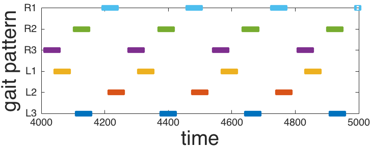
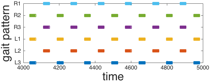
Figure 27: (Left to right) A solution of 24 ODEs for $\delta=0.014$ and ${c}_{i}$’s as in the first row of Table 3 and for $\delta=0.03$ and ${c}_{i}$’s as in the second row of Table 3. Note the approximate tetrapod and almost perfect tripod gaits.

Figures 28 (left to right) show the nullclines and corresponding phase planes of Equations (24) for the two different values of $\delta$. As Figure 28 (left) depicts, when the speed parameter is relatively small, there exist 4 fixed points: a sink which corresponds to a transition gait, a source and 2 saddle points. Figure 28 (right) shows that these fixed points persist as the speed parameter increases, but the sink now corresponds to a tripod gait. No bifurcation of fixed points occurs, although the topology of the nullclines changes.

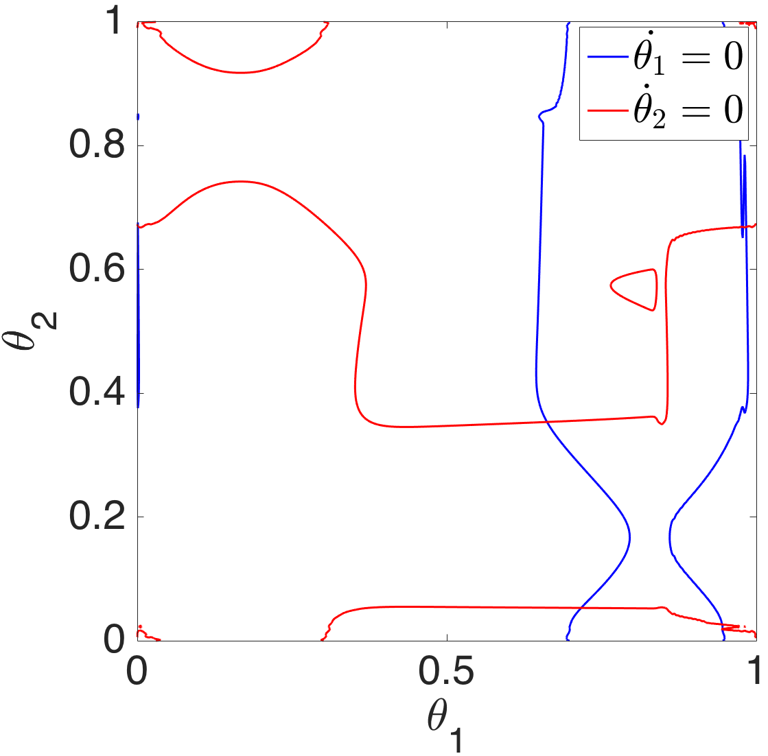
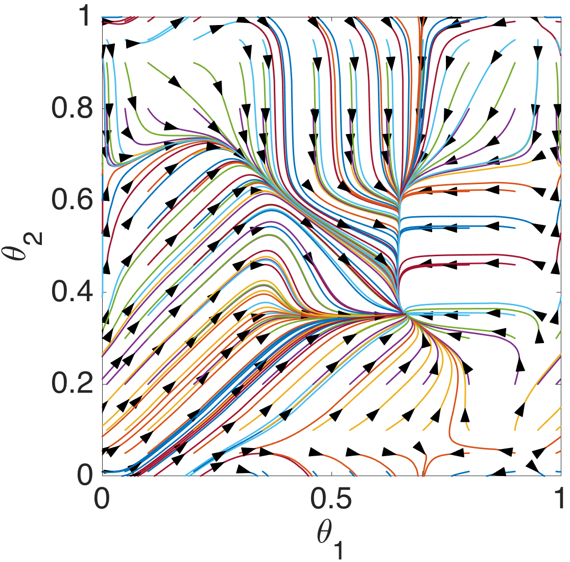
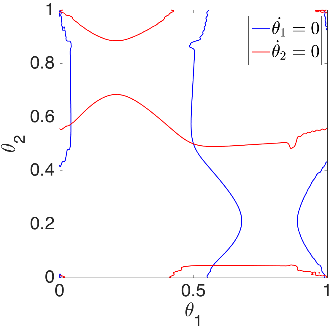
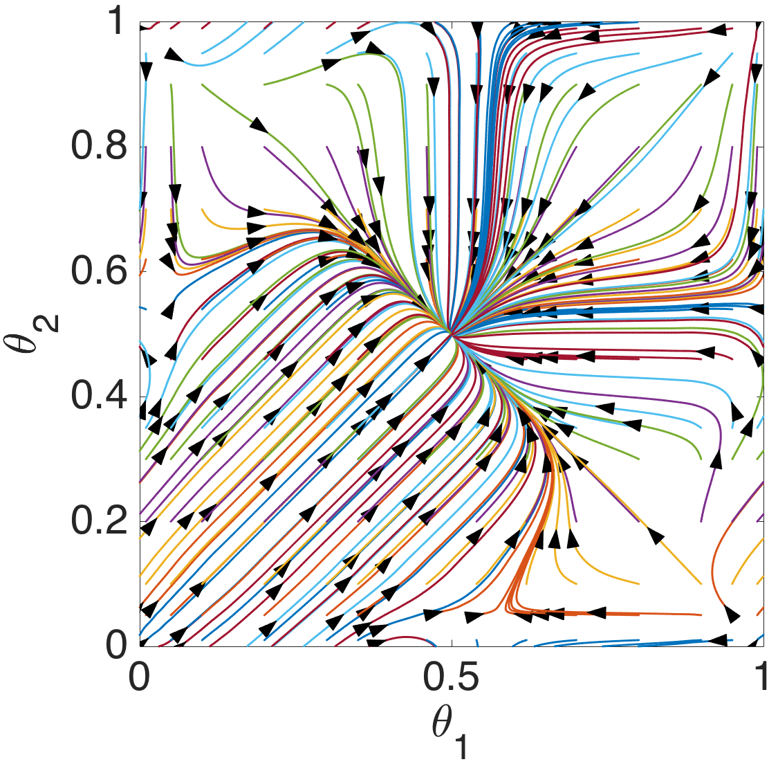
Figure 28: (Left to right) Nullclines and phase planes of Equations (24) for $\delta=0.014$ and ${c}_{i}$’s as in the first row of Table 3 (left pair); $\delta=0.03$ and ${c}_{i}$’s as in the second row of Table 3 (right pair). Note the close approximation to reflection symmetry at right due to almost perfect balance, ${c}_{1}\approx{c}_{2}\approx{c}_{3}$ and ${\alpha}=0.5269\approx 1/2$.

Note that the estimated coupling strengths in only the second row of Table 3 approximately satisfy the balance equation (26) and also ${c}_{1}\approx{c}_{2}\approx{c}_{3}$. Hence, as our analysis predicts, the system has 4 fixed points: a sink corresponding to a tripod gait, a source and 2 saddle points. Although the other estimated coupling strengths do not satisfy the balance equation (26), we still observe the existence of one sink which corresponds to a tetrapod gait (slow speed), a transition gait (medium speed), or a tripod gait (high speed). As discussed earlier, the balance equation is a necessary condition for the existence of tetrapod and tripod gaits but it is not sufficient. The estimated coupling strengths in Tables 2 and 3 (first row), provide counterexamples.

Remark 5.

The coupling strengths ${c}_{i}$ in Tables 2 and 3 are at most $O(1)$, the largest being $\approx 5.48$ in Table 3. From Figures 8 and 9 (second rows), the maxima of $\left|H\right|$ are $0.19$ (as $I_{ext}$ varies) and $0.4$ (as $\delta$ varies). Thus $\left|c_{i}H\right|$ takes maximum values of $0.19\times 1.15\approx 0.219$ in Table 2 and $0.4\times 5.48\approx 2.19$ in Table 3. For both sets of data, we observe transition from a stable (forward) tetrapod gait to a stable tripod gait as the speed parameter ${\xi}$ increases. However, the coupled frequency $\hat{\omega}$ should be less than the uncoupled frequency $\omega$, which does not hold in some cases.

8 Discussion

In this paper we developed an ion-channel bursting-neuron model for an insect central pattern generator based on that of [8]. We used this to investigate tetrapod to tripod gait transitions, at first numerically for a system of 24 ODEs describing cell voltages, ionic gates and synapses, and then for a reduced system of six coupled phase oscillators. This still presents a challenging problem, but by fixing contralateral phase differences, we further reduced to three ipsilaterally-coupled oscillators and thence to a set of ODEs defined on the 2-torus that describes phase differences between front and middle and hind and middle legs. This allowed us to study different sets of inter-leg coupling strengths as stepping frequency increases, and to find constraints on them that yield systems whose phase spaces are amenable to analysis.

Recent studies of different 3-cell ion-channel bursting CPG networks [25, 26, 27] share some common features with the current paper. Without explicitly addressing insect locomotion, or using phase reduction theory, the authors numerically extract Poincaré maps defined on 2-dimensional tori which have multiple stable fixed points corresponding to orbits with specific phase differences. In [27] they discuss transient control inputs that can move solutions from one stable state to another. A more abstract study of coupled cell systems with an emphasis on heteroclinic cycles that lie in “synchronous subspaces” appears in [28].

In addition to Propositions 1, 2, 3, 4 and Corollary 1, which characterize particular tetrapod and tripod solutions of the phase and phase-difference equations, our main results in Sections 4 and 7 illustrate the existence of these solutions and their stability types. Figures 10 and 14-16 display nullclines and phase portraits for systems with balanced coupling strengths, showing how a set of fixed points arrayed around a square astride the main diagonal $\theta_{1}=\theta_{2}$ on the 2-torus collapses to a single fixed point, corresponding to a stable tripod gait, as speed increases. Figures 23 and 24 illustrate nullclines and bifurcation diagrams for a Fourier series approximation of the coupling function. Finally, Figures 25-28 show gaits, nullclines and phase portraits for several cases in which coupling strengths were fitted to data from free running animals.

While details vary depending upon the coupling strengths, the results of Section 4 reveal a robust phenomenon in which a group of fixed points that include stable forward and backward tetrapod gaits converge upon and stabilize a tripod gait. This occurs even for coupling strengths that are far from balanced. For the coupling strengths derived from data in Section 7 (Figures 25-28), as stepping frequency increases and coupling strengths change there is still a shift from an approximate forward tetrapod to an approximate tripod gait, in which the tetrapod gaits disappear in saddle node bifurcations. In the final example (Figures 27 and 28 (right panels)) the tripod gait is almost ideal.

In Definition 1 we introduced 4 tetrapod gaits, two of which feature a wave traveling from front to hind legs. Such backward waves are not normally seen in insects and we excluded them from the gaits illustrated thus far. They do, however, appear as fixed points in the region $(\theta_{1},\theta_{2})=(T/3+{\eta},2T/3-{\eta})$ on the torus, which as shown in Proposition 8, are stable for some values of coupling strengths. We note that this backward wave in leg touchdowns does not imply backward walking, the study of which demands a more detailed model with motoneurons and muscles, to characterize different legs and leg joint angle sequences, as in e.g. [18].

For completeness, see Figure 29 for a backward tetrapod gait of the interconnected bursting neuron model, when $\delta=0.01$. The initial conditions are as follows:

$$v_{1}(0)=-40,\;v_{2}(0)=-40,\;v_{3}(0)=-30,\;v_{4}(0)=10,\;v_{5}(0)=5,\;v_{6}(0)=-20,$$ (54)

and for $i=1,\ldots,6$, $m_{i}$, ${w}_{i}$, and $s_{i}$ are as in Equation (11). The coupling strengths ${c}_{i}$ are as in Equation (8).

Figure 29: Interconnected bursting neuron model: backward tetrapod gait for $\delta=0.01$.

Recall from Section 5 (Figures 16 and 17), when ${\alpha}=0.95\approx 1$, a stable backward tetrapod gait exists, but a stable forward tetrapod exists for ${\alpha}=0.032\ll 1$. Since ${\alpha}=\frac{{c}_{4}}{{c}_{4}+{c}_{7}}$, and ${c}_{5}\approx{c}_{6}$ if ${c}_{1}\approx{c}_{2}\approx{c}_{3}$, this suggests that when couplings from front to hind legs are strong (${c}_{4},{c}_{6}\gg{c}_{7}$), we expect to see backward tetrapod gaits, but when couplings from hind to front legs are strong (${c}_{5},{c}_{7}\gg{c}_{4}$), forward tetrapod gaits would be observed. Similarly, in [29], a lamprey model suggested that the tail-to-head neural connections along the spinal cord would be stronger than those running from head to tail, despite the fact that the wave associated with swimming travels from head to tail. That prediction was later confirmed experimentally in [30]. See Figure 26 (left) for examples of coexisting stable backward and forward tetrapod gaits in a phase plane plot obtained from fitted fruit fly data. Backward tetrapod gaits have been observed in backward-walking flies, but have not been seen in forward-walking flies [31, Supplementary Materials, Figure S1].

In the introduction we mentioned related work of Yeldesbay et. al. [11, 12] in which a non-bursting half center oscillator model for the CPG contained in three ipsilateral segments is reduced to a set of ipsilateral phase oscillators with unidirectional coupling running from front to middle to hind and returning to front leg units. Tetrapod, tripod and transition gaits were also found in their work, although the cyclic architecture is strikingly different from our nearest neighbor coupling and it involves excitatory and inhibitory proprioceptive feedback. It is therefore interesting to see that similar gaits appear in both reduced models, although the bifurcations exhibited in [11, 12] appear quite different from those illustrated here in Figures (23) and (24). Moreover, gait transitions occur in response to changes in feedback as well as to changes in stepping frequency.

In summary, we have shown that multiple tetrapod gaits exist and can be stable, and described the transitions in which they approach tripod gaits as speed increases. In studying the phase reduced system on the 2-torus, we move from the special cases of Section 4, in which coupling strengths are balanced and other constraints apply, to the experimentally estimated data sets of Section 7 in which the detailed dynamics differ but tetrapod to tripod transitions still occur.

9 Appendix

Here, we review the theory of weakly coupled oscillators which can reduce the dynamics of each neuron to a single first order ODE describing the phase of the neuron. In Section 3, we applied this method to the coupled bursting neuron models to reduce the 24 ODEs to 6 phase oscillator equations.

Let the ODE

$$\dot{X}=f(X),\qquad X\in{\mathbb{R}}^{n},$$ (55)

describe the dynamics of a single neuron. In our model, $X=(v,m,{w},s)^{T}$ and $f(X)$ is as the right hand side of Equations (1). Assume that Equation (55) has an attracting hyperbolic limit cycle $\Gamma=\Gamma(t)$, with period $T$ and frequency ${\omega}=2\pi/T$.

The phase of a neuron is the time that has elapsed as its state moves around $\Gamma$, starting from an arbitrary reference point in the cycle. We define the phase of the periodically firing neuron at time $t$ to be

$$\phi(t)=\omega t+\bar{\phi}\quad\mbox{mod T}.$$ (56)

The constant $\bar{\phi}$, which is called the relative phase, is determined by the state of the neuron on $\Gamma$ at time $t=0$. Note that by the definition of phase, Equation (55) for a single neuron is reduced to the scalar equation

$$\frac{d\phi}{dt}=\omega,$$ (57)

while the dynamics of its relative phase are described by

$$\frac{d\bar{\phi}}{dt}=0.$$ (58)

Now consider the system of weakly coupled identical neurons

$$\dot{X}_{1}=f(X_{1})+\epsilon g(X_{1},X_{2}),$$ (59)

$$\dot{X}_{2}=f(X_{2})+\epsilon g(X_{2},X_{1}),$$

where $0<\epsilon\ll 1$ is the coupling strength and $g$ is the coupling function. For future reference, recall that neurons are coupled only via their voltage variables; see Equation (7). When a neuron is perturbed by synaptic currents from other neurons or by other external stimuli, its dynamics no longer remain on the limit cycle $\Gamma$, and the relative phase $\bar{\phi}$ is not constant. However, when perturbations are sufficiently weak, the intrinsic dynamics dominate, ensuring that the perturbed system remains close to $\Gamma$ with frequency close to $\omega$. Therefore, we can approximate the solution of neuron $j$ by

$$X_{j}(t)=\Gamma(\omega t+\bar{\phi}_{j}(t)),$$ (60)

where the relative phase $\bar{\phi}_{j}(t)$ is now a function of time $t$. Over each cycle of the oscillations, the weak perturbations to the neurons produce only small changes in $\bar{\phi}_{j}(t)$. These changes are negligible over a single cycle, but they can slowly accumulate over many cycles and produce substantial effects on the relative firing times. The goal now is to understand how the relative phases $\bar{\phi}_{j}(t)$ of the coupled neurons evolve.

To do this, we first review the concept of an infinitesimal phase response curve (iPRC), $Z(\phi)$, and then we show how to derive the phase equation given in Equation (14) from Equation (13). For details see [8, 32]; specifically, we borrow some material from [32].

Intuitively, an iPRC [33] of an oscillating neuron measures the phase shifts in response to small brief perturbations (Dirac $\delta$ function) delivered at different times in its limit cycle and acts like a Green’s function for the oscillating neurons. Below, we will give a precise mathematical definition of the iPRC and explain how we compute it in our model.

Suppose that a small brief rectangular current pulse of amplitude $\epsilon I$ and duration $\Delta t$ is applied to a neuron at phase $\phi$, i.e., the total charge applied to the cell by the stimulus is equal to $\epsilon I\Delta t$. Then the membrane potential $v$ changes by $\Delta v=\epsilon I\Delta t/C$. Depending on the amplitude and duration of the stimulus and the phase in the oscillation at which it is applied, the cell may fire sooner (phase advance) or later (phase delay) than it would have fired without the perturbation. For sufficiently small and brief stimuli, the neuron will respond in an approximately linear fashion, and the iPRC in the direction of $v$, denoted by $Z_{v}$, scales linearly with the magnitude of the current stimulus in the limit $\Delta v\to 0$:

$$Z_{v}(\phi):=\lim_{\Delta v\to 0}\frac{\Delta\phi(\phi)}{\Delta v}.$$ (61)

Note that $Z_{v}$ only captures the response to perturbations in the direction of the membrane potential $v$. However, such responses can be computed for perturbations in any direction in state space.

There is a one to one correspondence between phase $\phi$ and each point $x$ on the limit cycle $\Gamma$. The phase map $\Phi$ on $\Gamma$ is defined as follows.

$$\Phi(x(t)):=\phi(t)=\omega t+\bar{\phi}\quad\mbox{mod T},$$ (62)

which implies that

$$\nabla_{x}\Phi\cdot\dot{X}=\nabla_{x}\Phi\cdot f=\omega.$$ (63)

The phase map is well defined for all points on $\Gamma$. For any asymptotically stable limit cycle, we can extend the domain of the phase map to points in the domain of attraction of the limit cycle. If $x$ is a point on $\Gamma$ and $y$ is a point in a neighborhood of $\Gamma$, then we say that $y$ has the same asymptotic phase as $x$ if

$$\|X(t,x)-X(t,y)\|\to 0\qquad\mbox{as $t\to\infty$},$$

where $X(\cdot,x)$ is the unique solution of Equation (55) with initial condition $x$. Note that with $x\in\Gamma$, $X(t,x)=\Gamma(\omega t+\bar{\phi})$, for some $\bar{\phi}$. This means that the solution starting at the initial point $y$ in a sufficiently small neighborhood of $\Gamma$ converges to the solution starting at the point $x\in\Gamma$ as $t\rightarrow\infty$, so that $\Phi(x)=\Phi(y)$. The set of all points in the neighborhood of $\Gamma$ that have the same asymptotic phase as the point $x\in\Gamma$ is called the isochron for phase $\phi=\Phi(x)$ [33, 34].

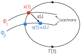
Figure 30: Isochrons and asymptotic phase.

Given the concepts of isochron and asymptotic phase, we show that the gradient of the phase map $\Phi$ is the vector iPRC, i.e., its components are the iPRCs for every variable in Equation (55). Suppose that, at time $t$, the neuron is in state $x(t)\in\Gamma(t)$ with corresponding phase $\phi_{1}(t)$:

$$\Phi(x(t))=\phi_{1}(t)=\omega t+\bar{\phi}_{1}(t).$$

At this time, it receives a small abrupt external perturbation $\epsilon U$ with magnitude $\epsilon$, where $U$ is the unit vector in the direction of the perturbation in state space. Immediately after the perturbation, the neuron is in the state $x(t)+\epsilon U$ and its new “asymptotic phase” is

$$\Phi(x(t)+\epsilon U)=\phi_{2}(t)=\omega t+\bar{\phi}_{2}(t).$$

See Figure 30 for an illustration. Using Taylor series,

$$\phi_{2}(t)-\phi_{1}(t)=\Phi(x(t)+\epsilon U)-\Phi(x(t))=\nabla_{x}\Phi(x(t))\cdot\epsilon U+O\left(\epsilon^{2}\right),$$ (64)

and dividing by $\epsilon,$ we obtain

$$\frac{\phi_{2}(t)-\phi_{1}(t)}{\epsilon}=\nabla_{x}\Phi(x(t))\cdot U+O\left(\epsilon\right),$$ (65)

and therefore, by the definition of iPRC, as $\epsilon\to 0$, the left hand side of Equation (65) is the iPRC at $\phi_{1}(t)$ in the direction of $U$:

$$Z(\phi_{1}(t))\cdot U=\nabla_{x}\Phi(x(t))\cdot U.$$ (66)

Hence, for any point on the limit cycle $\Gamma$, $Z=\nabla_{x}\Phi$.

The iPRCs can also be computed from an adjoint formulation [32, 35], which is the method adopted here. Specifically, the iPRC $Z$ is a $T$-periodic solution of the adjoint equation of Equation (55), i.e.,

$$\frac{dZ}{dt}=-[J_{f}(\Gamma)]^{T}\;Z,$$ (67)

subject to the constraint that makes $Z(\phi_{1}(t))$ normal to the limit cycle $\Gamma(t)$ at $t=0$:

$$Z(0)\cdot\Gamma^{\prime}(0)=0.$$ (68)

In Equation (67), $J_{f}(\Gamma)=D_{f}(\Gamma)$ is the linearization of Equation (55) around the limit cycle $\Gamma$ and $\Gamma^{\prime}(0)$ denotes the vector tangent to the limit cycle at time $t=0$: $\Gamma^{\prime}(0)=f(x(0))\mid_{x\in\Gamma}$. Note that the adjoint system (67) has the opposite stability of the original system (55), which has an asymptotically stable solution $\Gamma$. Thus, to obtain the unstable periodic solution of Equation (67), we integrate backwards in time from an arbitrary initial condition. To obtain the iPRC, we normalize the periodic solution using Equation (68).

There is a direct way to relate the gradient of the phase map to the solution of the adjoint equation (67). In fact, $\nabla_{x}\Phi(\Gamma(t))$ satisfies the adjoint equation (67) and the normalization condition Equation (68), [36]. Figure 8 and 9 (first rows) show $Z_{v}$, the first component of the vector iPRC $Z$ computed by the adjoint method, of the bursting neuron model for different values of $\delta$, and $I_{ext}$, respectively.

Now consider the system of weakly coupled identical neurons introduced in Equation (59). As we discussed earlier, our goal is to understand how the relative phase $\bar{\phi}_{j}(t)$ of the coupled neurons evolves slowly in time. For $i=1,2$, let $X_{i}(t)$ be solutions of Equation (59) with corresponding phases

$$\phi_{i}(t):=\Phi(X_{i}(t))=\omega t+\bar{\phi}_{i}(t).$$

Then by taking the derivative of $\phi_{i}$ and using Equations (59), (60), (63), and (66), we obtain:

$$\displaystyle\frac{d\phi_{i}}{dt}(t) =\nabla_{x}\Phi(X_{i}(t))\cdot\dot{X}_{i}$$ (69a)

$$=\nabla_{x}\Phi(X_{i}(t))\cdot\left[f(X_{i}(t))+\epsilon g(X_{i},X_{j})\right]$$ (69b)

$$\approx\nabla_{x}\Phi(\Gamma(\omega t+\bar{\phi}_{i}(t)))\cdot\left[f(\Gamma(\omega t+\bar{\phi}_{i}(t)))+\epsilon g(\Gamma(\omega t+\bar{\phi}_{i}(t)),\Gamma(\omega t+\bar{\phi}_{j}(t)))\right]$$ (69c)

$$=\omega+\epsilon Z(\Gamma(\omega t+\bar{\phi}_{i}(t)))\cdot g(\Gamma(\omega t+\bar{\phi}_{i}(t)),\Gamma(\omega t+\bar{\phi}_{j}(t))).$$ (69d)

Using the change of variables $\phi_{i}(t)=\omega t+\bar{\phi}_{i}(t)$, we get the following dynamics for ${d\bar{\phi}_{i}}/{dt}$

$$\frac{d\bar{\phi}_{i}}{dt}(t)=\epsilon Z(\Gamma(\omega t+\bar{\phi}_{i}(t)))\cdot g(\Gamma(\omega t+\bar{\phi}_{i}(t)),\Gamma(\omega t+\bar{\phi}_{j}(t))).$$ (70)

Now letting $\tilde{t}:=\omega t+\bar{\phi}_{i}(t)$ and taking the average of the right hand side of Equation (70) over one unperturbed period and using the Averaging Theorem [21, Section 4.1], we obtain the following equation for the relative phase $\bar{\phi}_{i}$.

$$\frac{d\bar{\phi}_{i}}{dt}=\frac{\epsilon}{T}\int_{0}^{T}Z(\Gamma(\tilde{t}))\cdot g(\Gamma(\tilde{t}),\Gamma(\tilde{t}+\bar{\phi}_{j}(t)-\bar{\phi}_{i}(t)))\;d\tilde{t}=:\epsilon H(\bar{\phi}_{j}(t)-\bar{\phi}_{i}(t)),$$ (71)

where

$$H=H(\theta)=\frac{1}{T}\int_{0}^{T}Z(\Gamma(\tilde{t}))\cdot g(\Gamma(\tilde{t}),\Gamma(\tilde{t}+\theta))\;d\tilde{t},$$

is the coupling function: the convolution of the synaptic current input to the neuron via coupling $g$ and the neuron’s iPRC $Z$. Using $\phi_{i}(t)=\omega t+\bar{\phi}_{i}(t)$ and Equation (71), we can write the phase equation of each neuron instead of relative phase equations,

$$\frac{d\phi_{i}}{dt}(t)=\omega+\epsilon H(\phi_{j}(t)-\phi_{i}(t)),$$ (72)

where $\epsilon$ denotes the coupling strength (cf. Equation (71)).

References

- [1] D.M. Wilson. Insect walking. Ann. Rev. Entomol., pages 103–122, 1966.
- [2] D. Graham. Pattern and control of walking in insects. Adv. Insect Physiology, 18:31–140, 1985.
- [3] C.S. Mendes, I. Bartos, T. Akay, S. Márka, and R.S. Mann. Quantification of gait parameters in freely walking wild type and sensory deprived Drosophila melanogaster. eLife, 2:e00231, 2013.
- [4] E. Couzin-Fuchs, T. Kiemel, O. Gal, A. Ayali, and P. Holmes. Intersegmental coupling and recovery from perturbations in freely running cockroaches. J. Exp. Biol., 218(2):285–297, 2015.
- [5] A. Ayali, A. Borgmann, A. Buschges, E. Couzin-Fuchs, S. Daun-Gruhn, and P. Holmes. The comparative investigation of the stick insect and cockroach models in the study of insect locomotion. Current Opinion in Insect Science, 12:1 – 10, 2015.
- [6] M. Golubitsky, I. Stewart, P-L. Buono, and J.J. Collins. Symmetry in locomotor central pattern generators and animal gaits. Nature, 401:693–695, 1999.
- [7] J.J. Collins and I.N. Stewart. Coupled nonlinear oscillators and the symmetries of animal gaits. Journal of Nonlinear Science, 3(1):349–392, Dec 1993.
- [8] R.M. Ghigliazza and P. Holmes. A minimal model of a central pattern generator and motorneurons for insect locomotion. SIAM J. Appl. Dyn. Sys., 3(4):671–700, 2004.
- [9] F. Delcomyn. The locomotion of the cockroach Periplaneta americana. J. Exp. Biol., 54 (2):725–744, 1971.
- [10] K.G. Pearson and J.F. Iles. Nervous mechanisms underlying intersegmental co-ordination of leg movements during walking in the cockroach. J. Exp. Biol., 58:725–744, 1973.
- [11] A. Yeldesbay, P. Holmes, T. Tóth, and S. Daun. Phase reduction of an inter-segmental network model of stick insect locomotion. 2016. Poster presented at Advances in the collective behaviour of complex systems, University of Potsdam, Sept. 1-3.
- [12] A. Yeldesbay, T. Tóth, and S. Daun. Phase reduction of an inter-segmental network model of multi-legged locomotion. In preparation, 2017.
- [13] R.M. Ghigliazza and P. Holmes. Minimal models of bursting neurons: The effects of multiple currents and timescales. SIAM J. Appl. Dyn. Sys., 3(4):636–670, 2004.
- [14] E. Marder and D. Bucher. Central pattern generators and the control of rhythmic movements. Current Biology, 11(23):R986 – R996, 2001.
- [15] A.J. Ijspeert. Central pattern generators for locomotion control in animals and robots: A review. Neural Networks, 21(4):642 – 653, 2008.
- [16] K.G. Pearson and J.F. Iles. Discharge patterns of coxal levator and depressor motoneurones of the cockroach, Periplaneta americana. J. Exp. Biol., 52:139–165, 1970.
- [17] K.G. Pearson. Central programming and reflex control of walking in the cockroach. J. Exp. Biol., 56:173–193, 1972.
- [18] T.I. Tóth, S. Knops, and S. Daun-Gruhn. A neuromechanical model explaining forward and backward stepping in the stick insect. J. Neurophysiol., 107:3267–3280, 2013.
- [19] P. Ashwin, S. Coombes, and R. Nicks. Mathematical frameworks for oscillatory network dynamics in neuroscience. J. Math. Neurosci., 6 (2):1–92, 2016.
- [20] C. Zhang and T.J. Lewis. Robust phase-waves in chains of half-center oscillators. J. Math. Biol., 74(7):1627–1656, 2017.
- [21] J. Guckenheimer and P. Holmes. Nonlinear Oscillations, Dynamical Systems, and Bifurcations of Vector Fields. Springer-Verlag, 6th edition, 2002.
- [22] E. Couzin. Analysis of free-walking fly data. Unpublished notes, 2016.
- [23] A. Dhooge, W. Govaerts, and Yu.A. Kuznetsov. Matcont: A Matlab package for numerical bifurcation analysis of ODEs. ACM TOMS, 29:141–164, 2003.
- [24] D. Alspach and H. Sorenson. Nonlinear Bayesian estimation using Gaussian sum approximations. IEEE Transactions on Automatic Control, 17(4):439–448, 1972.
- [25] J. Wojcik, J. Schwabedal, R. Clewley, and A.L. Silnikov. Key bifurcations of bursting polyrhythms in 3-cell central pattern generators. PLoS ONE, 9 (4):e92918, 2014.
- [26] R. Barrio, M. Rodríguez, S. Serrano, and A. Silnikov. Mechanism of quasi-periodic lag jitter in bursting rhythms by a neuronal network. European Phys. Let., 112:38002, 2015.
- [27] A. Lozano, M. Rodríguez, and R. Barrio. Control strategies of 3-cell central pattern generator via global stimuli. Scientific Reports, 6:23622, 2016.
- [28] M. Aguiar, P. Ashwin, A. Dias, and M. Field. Dynamics of coupled cell networks: Synchrony, heteroclinic cycles and inflation. J. Nonlinear Sci., 21:271–323, 2011.
- [29] G.B. Ermentrout and N. Kopell. Frequency plateaus in a chain of weakly coupled oscillators. SIAM Journal on Mathematical Analysis, 15(2):215–237, 1984.
- [30] K.A. Sigvardt and T.L. Williams. Models of central pattern generators as oscillators: The lamprey locomotor CPG. Seminars in Neuroscience, 4(1):37 – 46, 1992.
- [31] S.S. Bidaye, C. Machacek, Y. Wu, and B.J. Dickson. Neuronal control of drosophila walking direction. Science, 344:97–101, 2014.
- [32] M.A. Schwemmer and T.J. Lewis. The theory of weakly coupled oscillators. In N.W. Schultheiss, A.A. Prinz, and R.J. Butera, editors, Phase Response Curves in Neuroscience: Theory, Experiment, and Analysis, pages 3–31. Springer, New York, 2012.
- [33] A.T. Winfree. The Geometry of Biological Time, volume 12 of Interdisciplinary Applied Mathematics. Springer-Verlag, New York, second edition, 2001.
- [34] J. Guckenheimer. Isochrons and phaseless sets. J. Math. Biol., 1:259–273, 1975.
- [35] G.B. Ermentrout and D. Terman. Mathematical Foundations of Neuroscience. Springer, New York, 2010.
- [36] E. Brown, J. Moehlis, and P. Holmes. On the phase reduction and response dynamics of neural oscillator populations. Neural Comput., 16(4):673–715, April 2004.