Effect of lateral tip motion on multifrequency atomic force microscopy

Abstract

In atomic force microscopy (AFM), the angle relative to the vertical ($\theta_{i}$) that the tip apex of a cantilever moves is determined by the tilt of the probe holder, and the geometries of the cantilever beam and actuated eigenmode $i$. Even though the effects of $\theta_{i}$ on static and single-frequency AFM are known (increased effective spring constant, sensitivity to sample anisotropy, etc.), the higher eigenmodes used in multifrequency force microscopy lead to additional effects that have not been fully explored. Here we use Kelvin probe force microscopy (KPFM) to investigate how $\theta_{i}$ affects not only the signal amplitude and phase, but can also lead to behaviors such as destabilization of the KPFM voltage feedback loop. We find that longer cantilever beams and modified sample orientations improve voltage feedback loop stability, even though variations to scanning parameters such as shake amplitude and lift height do not.

The development of specialized cantilever probes enabled atomic force microscopy (AFM)Binnig1986 . Later, it was realized that the holder tilts the cantilever and the trajectory of the tip apex which both increases the effective static spring constant and causes the phase of Amplitude Modulation (AM) AFM to be sensitive to both the anisotropy and slope of samplesMarcus2002 ; DAmato2004 ; Heim2004 ; Hutter2005a . For higher eigenmodes $i$, the angle between the tip apex trajectory and the vertical axis ($\theta_{i}$) also depends the geometries of the cantilever and eigenmode, so that recent experiments were able to use eigenmodes with different $\theta_{i}$ to probe forces in several directionsKawai2010a ; Sigdel2013 ; Reiche2015 ; Meier2016 ; Huang2017 ; Naitoh2017 . Bimodal AFM, in which two eigenmodes are driven by excitation of the cantilever base, was used for most of these experiments, but it is only one of many multifrequency techniquesNonnenmacher1991 ; Jesse2007 ; Platz2008 ; Tetard2010 ; Garcia2012a ; Ebeling2013b ; Zerweck2005 ; Rajapaksa2011 ; Sugawara2012 ; Arima2015 ; Garrett2016 ; Tumkur2016 ; Jahng2016 ; Ambrosio2017 , and the effects of $\theta_{i}$ have not yet been explored for the general multifrequency case.

Sideband multifrequency AFM methods are promising ways to investigate optoelectronic materials and devices at the nanoscaleZerweck2005 ; Rajapaksa2011 ; Sugawara2012 ; Arima2015 ; Garrett2016 ; Tumkur2016 ; Jahng2016 ; Ambrosio2017 . In order to eliminate long-range artifacts and improve spatial resolution, they drive a signal by mixing a modulated tip-sample force with piezo-driven cantilever oscillations. A prominent sideband method is photo-induced force microscopy (PIFM), which has been used for nanoscale imaging of Raman spectraRajapaksa2011 , nanoparticle resonancesTumkur2016 , and refractive index changesAmbrosio2017 . However, there is considerable debate about how to extract quantitative data from PIFM scansJahng2016 ; Tumkur2016 ; Ambrosio2017 because it is unclear how the force couples into the probe and optical forces themselves are difficult to characterize a priori.

Because the electrostatic force is well-characterized and controllable compared to optical forces, it offers an opportunity to test the sideband actuation technique. Frequency Modulation (FM) and Heterodyne (H) Kelvin probe force microscopy (KPFM) are sideband methods that use the electrostatic force to drive cantilever oscillations, which are in turn input into a feedback loop that measures the tip-sample potential difference. In a recent experiment, height variation of around 10 nm destabilized the H-KPFM voltage feedback loop, but FM-KPFM scans were stable for variations of over 100 nmGarrett2017a . Because FM- and H-KPFM are primarily distinguished by the eigenmode used to amplify the KPFM signal, the cause of their qualitatively different behavior likely originates from the geometry of the eigenmodes. Moreover, the details of cantilever dynamics have been shown to be critical to understanding AM-KPFMElias2011 ; Satzinger2012 , a much simpler technique that drives and detects its signal at a single frequency, and which can be used for comparison.

Figure 1: The tip apex moves at an angle relative to the vertical for each eigenmode $i$ ($\theta_{i}$), which depends on the angle of the probe holder ($\theta_{\text{holder}}$), the geometry of the cantilever, and the geometry of the eigenmode ($\Phi_{i}$). The inset shows the tip apex with the first eigenmode excited ($i$=1), in which the amplitude of the eigenmode ($Y_{1}$), the tip apex displacement ($\vec{r}_{1}$), and $\theta_{1}$ are labeled.

In this letter, we use KPFM measurements to answer the questions: (a) how does the $\theta_{i}$ of each eigenmode affect the signals of KFPM, (b) why does the KPFM feedback instability differ between H- and FM-KPFM, and (c) how do the effects of $\theta_{i}$ appear in sideband multifrequency force microscopy methods?

The motion of a cantilever beam can be expressed as a sum of eigenmodes, each a solution to the Euler-Bernoulli beam equationButt1995 ; Lozano2009 :

$$z_{\text{cant}}(x,t)=\sum_{i=1}^{\infty}Y_{i}(t)\Phi_{i}(x),$$ (1)

where $Y_{i}(t)$ contains the time-dependence, $\Phi_{i}$ is the shape of the $i$th cantilever beam eigenmode (normalized so that $\Phi_{i}(L)=1$, where $L$ is the length of the cantilever beam), and $z_{\text{cant}}$ is the displacement of the cantilever beam (see figure 1). To maintain generality, the exact form of $\Phi_{i}$ is not specified until the numerical evaluation of $\theta_{i}$, at which point the solution for a rectangular cantilever beam is usedButt1995 ; Lozano2009 . Thus the following analysis holds even for non-rectangular cantilever beams and probes with large tip cones, both which may have atypical $\Phi_{i}$Tung2010 ; Labuda2016 .

To calculate the trajectory of the tip apex, the probe is characterized by its tip cone height $h$, contact angle $\delta$, and contact position $x_{t}$ (figure 2). The position of the tip apex is the location of base of the tip cone {$x_{t},Y_{i}\Phi_{i}(x_{t})$} plus the position of the tip apex relative to the base of tip cone, {$h\cos(\xi(Y_{i})-\delta),h\sin(\xi(Y_{i})-\delta)$}, where $\xi(Y_{i})=\tan^{-1}(Y_{i}\partial_{x}\Phi_{i}(x_{t}))$ is the angle of the vector normal to the cantilever at $x_{t}$. Because the probe is held at an angle $\theta_{\text{holder}}$ (here, 0.2 radians), the displacement of the tip apex from equilibrium becomes, in the small oscillation limit ($Y_{i}\ll L$):

$$\vec{r}_{i} =\mathbf{R}\bigg{[}\begin{matrix}h(\cos(\xi(Y_{i})-\delta)-\cos(\delta))\\ Y_{i}\Phi_{i}(x_{t})+h(\sin(\xi(Y_{i})-\delta)+\sin(\delta))\end{matrix}\bigg{]},$$ (2)

where $\mathbf{R}=\left[\begin{smallmatrix}\cos(\theta_{\text{holder}})&\sin(\theta_{\text{holder}})\\ -\sin(\theta_{\text{holder}})&\cos(\theta_{\text{holder}})\end{smallmatrix}\right]$ is a 2D rotation matrix around the base of the cantilever beam. For a single eigenmode in the $Y_{i}\ll L$ limit, the tip apex moves in a straight line at an angle with respect to the vertical:

$$\theta_{i}=\lim_{Y_{i}/L\rightarrow 0}\cos^{-1}\big{(}\vec{r}_{i}\cdot(Y_{i}\hat{z})\big{)}.$$ (3)

Note that equations 2 and 3 imply that much of the trajectory of the tip apex is in the $\hat{x}$ direction, even for very small excitations. For example, a 10 nm amplitude excitation of the first eigenmode of the cantilever beam in figure 2b causes the tip apex to move $\approx 3.9$ nm in the $\hat{x}$ direction and 8.6 nm in the $\hat{z}$ direction. Because the potential energy of an eigenmode must be the same whether the motion of the end of cantilever beam ($\Phi_{i}(L)$) or the tip apex ($\vec{r}_{i}$) is considered, an effective spring constant ($k_{i}^{\text{eff}}$) for forces acting on the tip apex parallel to $\vec{r}_{i}$ (perpendicular forces excite only eigenmodes $\neq i$) can be definedReiche2015 :

$$k_{i}^{\text{eff}} =\lim_{Y_{i}/L\rightarrow 0}\frac{Y_{i}^{2}}{|\vec{r}_{i}(Y_{i})|^{2}}k_{i},$$ (4)

where $k_{i}$ is the spring constant for an upward force acting at $x=L$Melcher2007 .

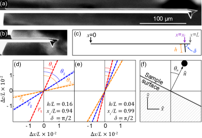
Figure 2: Cantilever geometry determines the direction of the tip apex motion. (a,b) SEM images show cantilevers of length 350 $\mu$m and 90 $\mu$m, respectively ($\mu$masch, CSC37/Pt-B and NSC35/Pt-B). (c) Each cantilever is characterized by its tip cone height $h$, contact position $x_{t}$, contact angle $\delta$, and length $L$. (d,e) The full calculation of $\vec{r}_{i}$ (solid line, equation 2) and linear approximation (dashed line, equation 3) show agreement. For each eigenmode, $\theta_{i}$ is greater for the short cantilever than for the long cantilever. (f) The slope of the sample is characterized by its normal vector ($\hat{n}$) and the angle it makes with the vertical ($\theta_{n}$).

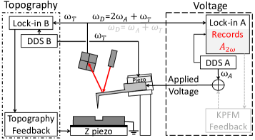
Figure 3: An AC voltage, $V_{AC}$, is applied to the cantilever at frequency $\omega_{A}$, while tip-sample separation is controlled by piezo-driven oscillation at frequency $\omega_{T}$ and the sample is grounded. The oscillations at $\omega_{T}$ mix with the electrostatic force driven by $V_{AC}$ at frequency $\omega_{A}$ to drive the tip apex at the detection frequency, $\omega_{D}$, which is amplified by one of the cantilever’s resonance frequencies and detected by a lock-in amplifier. When KPFM feedback is used, the grey signal paths are added to the circuit, and $\omega_{A}=(\omega_{D}-\omega_{T})/2$ is changed to $\omega_{A}=\omega_{D}-\omega_{T}$.

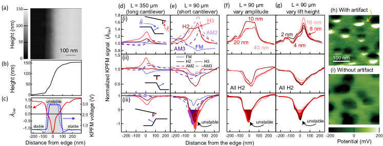
Figure 4: (a,b) The height of a trench that is scanned with KPFM ($128^{2}$ pixels, 500 nm/s). (c) Where the normalized signal ($\tilde{A}_{2\omega}$, red) becomes negative, the KPFM voltage with feedback on (blue) becomes unstable and approaches the limit imposed on the feedback loop, for both trace (solid) and retrace (dashed). Long (d) and short (e-g) cantilever beams scan across the trench edge in three different orientations: down (i, $\theta_{n}<0$), parallel to (ii), and up the slope (iii, $\theta_{n}>0$). In (i,ii), $\tilde{A}_{2\omega}$ remains positive for all methods, but in (iii) all methods except FM-KPFM contain a negative portion for the short cantilever beam. (f,g) Varying scan parameters such as $A_{T}$ (used for topography control) and lift height are not sufficient to prevent $\tilde{A}_{2\omega}$ < 0. The different scanning modes are labeled by a prefix (eg. ‘H’ for H-KPFM) and a number indicating the eigenmode used to amplify the signal, except for FM-KPFM, which always uses the first eigenmode. (h) An artifact is present in an H-KFPM scan of Au nanoparticles on indium tin oxide when the signal is amplified by the second eigenmode of the short cantilever beam. (i) When the long cantilever beam is used to scan other Au nanopaticles on the same sample, the artifact is eliminated.

Table 1: Cantilever resonance frequencies

L ($\mu$m)	$\frac{\omega_{1}}{2\pi}$ (MHz)	$\frac{\omega_{2}}{2\pi}$	$\frac{\omega_{3}}{2\pi}$	$\frac{\omega_{4}}{2\pi}$	$\frac{\omega_{5}}{2\pi}$	$\frac{\omega_{6}}{2\pi}$	$\frac{\omega_{7}}{2\pi}$
90	0.25	1.62	4.58	-	-	-	-
350	0.02	0.13	0.37	0.72	1.20	1.79	2.50

The tip apex trajectory affects AFM techniques that use a modulated tip-sample force $\vec{F}_{\text{dir}}$ to actuate the cantilever either directly or through sideband coupling while relying on piezo-driven oscillation with amplitude $A_{T}$ at frequency $\omega_{T}$ for topography control (here, $\omega_{T}=\omega_{1}$ in table 1 is used). Sideband techniques generate a signal by modulating a separation-dependent force $\vec{F}_{\text{dir}}$ at frequency $\omega_{M}$, which is then mixed with the piezo-driven oscillations, typically $A_{T}$. Here, the resonance frequency used for detection determines the modulation frequency $\omega_{M}=\omega_{i}-\omega_{T}$ (table 1). By using the force gradient, sideband methods exclude the non-local effects of the cantilever beam that are present when $\vec{F}_{\text{dir}}$ is used for direct actuation, such as in AM-KPFMZerweck2005 ; Sugawara2012 ; Jahng2016 .

To confirm that the cantilever beam’s contribution to the total force is small even when higher eigenmodes are used, the force on the beam is computed for both direct actuation ($-\partial U/\partial Y_{i}$) and sideband actuation ($-\partial^{2}U/\partial Y_{i}^{2}$), where $U$ is the electrostatic potential energy between the probe and the surface evaluated using the proximity force approximation and the geometry of the longer probe. The contribution from the tip apex is calculated by modeling it as a 30 nm radius sphere 10 nm above the surface. The percent of the signal originating from the cantilever beam using direct actuation is found to be 17-53% for the first seven eigenmodes, while with sideband actuation 0.1-0.2% of the signal originates from the beam. The small contribution from the beam validates the approximation that the electrostatic force acts on the tip apex for sideband actuation of higher eigenmodes.

In the small-oscillation approximationJahng2016 ; Garrett2016 , the force driving sideband oscillation is $\vec{F}_{\text{side}}\cos(\omega_{D}t)$, where

$$\vec{F}_{\text{side}}=\partial_{d}\vec{F}_{\text{dir}}\frac{A_{T}}{2}\cos(\theta_{i}-\theta_{n}),$$ (5)

in which $d$ is the tip-sample separation, $\omega_{D}$ is the detection frequency, and the $\cos(\theta_{i}-\theta_{n})$ factor originates from the angle between the trajectory of the tip apex and the force vector (parallel to $\hat{n}$). The displacement of the tip apex at $\omega_{D}$ is then $\vec{r}_{j}(t)=A_{D}\cos(\omega_{D}t)\hat{r}_{j}$, where eigenmode $j$ is driven and the signal detected by the lock-in amplifier is

$$A_{D} =\frac{Q_{j}}{k^{\text{eff}}_{j}}\vec{F}\cdot\hat{r}_{j},$$ (6)

for both the sideband and direct driving forces (figure 3). A change in the sign of $A_{D}$ corresponds to a phase shift by $\pi$ radians.

The interplay of $\theta_{j}$ and sample slope can then be observed in the signal $A_{D}$ normalized by the its value on a flat surface ($\tilde{A}_{D}\equiv\frac{A_{D}}{A_{D}(\theta_{n}=0)}$):

$$\tilde{A}_{D}^{\text{dir}} =\frac{\cos(\theta_{j}-\theta_{n})}{\cos(\theta_{j})},$$ (7)

$$\tilde{A}_{D}^{\text{side}} =\frac{\cos(\theta_{n}-\theta_{j})\cos(\theta_{n}-\theta_{i})}{\cos(\theta_{j})\cos(\theta_{i})},$$ (8)

where it is assumed that $\hat{n}$ is in the x-z plane and $\theta_{i},\theta_{j}\neq\pm\pi/2$. Note that if $|\theta_{i}-\theta_{n}|>\frac{\pi}{2}>\theta_{i}$, $\tilde{A}_{D}$ changes sign.

Equations 7 and 8 predict how the geometry of tip apex motion causes scanning probe methods to be sensitive to sample slope. To test the equations, a silicon trench is fabricated using e-beam lithography to pattern a 2 $\mu$m $\times$ 100 $\mu$m line on a silicon wafer which is then etched using reactive ion etching (RIE) and coated with 5 nm of chromium for conductivity. The edges of the trench are imaged, in attractive mode Paulo2002 , (Cypher, Asylum Research), trace and retrace images are averaged, and each column of pixels is summed and averaged (figure 4a,b).

In the static limit, when an AC voltage is applied to a probe at frequency $\omega_{A}$, the tip-sample electrostatic force has components at three frequenciesNonnenmacher1991 ; Zerweck2005 : $\vec{F}_{\text{es}}=\vec{F}_{DC}+\vec{F}_{\omega}\cos(\omega_{A}t)+\vec{F}_{2\omega}\cos(2\omega_{A}t).$ Either $\vec{F}_{\omega}$ or $\vec{F}_{2\omega}$ can be used in equation 5 to drive the sideband signal by choosing $\omega_{M}=\omega_{A}$ or $2\omega_{A}$, respectively. The signal then depends on the gradient of the original modulation forceZerweck2005 ; Sugawara2012 ; Miyahara2017 . For FM-KPFM, $\omega_{A}\ll\omega_{1}$Zerweck2005 . Closed loop KPFM measures the contact potential difference between the probe and sample using a feedback loop to nullify a signal driven by the force $\vec{F}_{\omega}$. Alternatively, open loop KPFM uses oscillation driven by $\vec{F}_{2\omega}$ combined with the $\vec{F}_{\omega}$ signal to estimate the potential difference $\Delta V$ from the relationship between the forces $\vec{F}_{2\omega}=\vec{F}_{\omega}V_{AC}/(4\Delta V)$Takeuchi2007 ; Collins2015 . The relationship between $\vec{F}_{2\omega}$ (which drives $A_{2\omega}$ according to equation 6) and KPFM feedback loop itself can be seen in figure 4c: the feedback becomes unstable at locations where $A_{2\omega}$ changes sign. Moreover, any change in $A_{2\omega}$ makes KPFM susceptible to topographic cross-talkBarbet2014 . The signal is driven by $\vec{F}_{2\omega}$ because it reveals the behavior of the KPFM feedback loop, without requiring feedback to be used and is not susceptible to patch potentials or tip change.

The effect of slope is revealed by observing how the normalized signal ($\tilde{A}_{2\omega}$) changes as the tip apex approaches an edge of the trench at different orientations, for AM-, FM- and H-KPFM with the first three eigenmodes of each cantilever, and $V_{AC}$ = 3 V. In figure 4 the trench edge is crossed with three different orientations: (i) the vector from the base of the cantilever beam to its tip apex points down the slope ($\theta_{n}>0$, from the higher to the lower level) (ii) parallel to the slope ($\hat{n}$ out of plane) and (iii) up the slope ($\theta_{n}<0$). One trend predicted by equation 8 is observed: $\tilde{A}_{2\omega}$ tends to increase as $\theta_{n}$ increases. However, the decrease of $\tilde{A}_{2\omega}$ is greater for the short cantilever beam than for the long cantilever beam. For the short cantilever beam, the $\theta_{n}<0$ edge leads to $\tilde{A}_{2\omega}<0$ for every technique except FM-KPFM.

Other scan parameters affect $\tilde{A}_{2\omega}$ much less. $A_{T}$, used for topography control, is varied from 10 to 40 nm, but the shape of $\tilde{A}_{2\omega}$ retains a negative portion as the $\theta_{n}<0$ edge is crossed. Similarly, using a two-pass method and varying the lift height from 2 nm to 16 nm does not prevent $\tilde{A}_{2\omega}<0$ at the $\theta_{n}<0$ edge. Thus, if KPFM feedback is unstable for geometric reasons, adjustments to the scan settings do not typically stablize it.

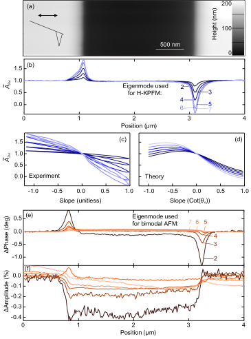
Figure 5: (a) A cantilever scans, using H-KPFM, across a 2 $\mu$m wide chromium-coated silicon trench (64$\times$256 pixels, 800 nm/s). (b) On the downward slope (left), the normalized signal $\tilde{A}_{2\omega}$ becomes larger, but on the upward slope (right), the signal decreases. (c) Measured and (d) predicted values of $\tilde{A}_{2\omega}$ are plotted against the local slope of the trench. Higher eigenmodes tend to show a greater change with slope, as predicted from their larger $\theta_{i}$. Bimodal AFM is also used to scan across the surface, while biased to 3 V. (e) The change in phase shows peaks at the edges, but unlike the H-KPFM case, the relative amplitude of the phase change decreases for higher eigenmodes, because the of increased $k^{\text{eff}}_{i}$. (f) The amplitude decreases in the middle of the trench, but not at the edges, and changes by $<0.5\%$.

To test the predictions with a wider range of $\theta_{i}$, the trenches are scanned again with the long probe in H-KPFM mode using the first eigenmode for topography control and amplifying the $\vec{F}_{2\omega}$ signal with eigenmodes 2-7 (ie. $\omega_{A}=\omega_{M}/2=(\omega_{i}-\omega_{1})/2$, so that $\omega_{D}=\omega_{i}$ for 2$\leq i\leq$7, table 1). Because each eigenmode has a slightly greater $\theta_{i}$ than the one before it (ie. $\theta_{i+1}>\theta_{i}$), equation 8 predicts that the effect of sample slope is greater for the higher eigenmodes than the lower ones, and the experiment confirms this trend, although the seventh eigenmode changes less than the sixth (figure 5b-d). The experimental data do not all fall on a single line (figure 5c), perhaps because the region on the sample from which the $\vec{F}_{2\omega}$ force originates deviates from the single-slope assumption. For eigenmodes 3-7, the data agree better with equation 8, which has no free parameters, than with the null hypothesis that the signal does not depend on slope, thus confirming that the direction of the force affects how it drives the tip apex. However, equation 8 tends to underestimate $\tilde{A}_{2\omega}$, particularly for slopes $<-0.5$, which suggests that other factors, such as the tip cone and changes to the piezo-driven oscillation, $A_{T}$, may also matter. An initial test of effect of slope on piezo-driven oscillation with bimodal AFM shows a change in the phase at the edges of the trench (figure 5e,f). Because the sideband excitation technique is similar for different forces, the results here indicate that $\theta_{i}$ affects the whole class of methods.

The direction of the tip apex trajectory depends on cantilever geometry and the eigenmodes used, and influences sideband multifrequency force microscopy methods. It can even change the sign of the signal, which leads to feedback instability in KPFM. The results here show that considerable topographic restrictions exist for multifrequency methods when short cantilevers are used. Because short cantilevers enable faster scanning than long cantileversWalters1996a , the restriction amounts to a speed limitation for any given roughness. Because the equations above separate the calculation of $\theta_{i}$ (1-4) from the analysis of the sideband signal (5-8), either portion can be combined with numerical methods to account for non-rectangular cantilever beams, or non-analytic forces. Knowledge of the effect of geometry will assist in the development of additional multifrequency methods and will make the interpretation of current methods more accurate. In particular, the improved stability of KPFM will enable high resolution voltage mapping of rough or textured surfaces, which will allow for improved nanoscale characterization of optoelectronic structures such as solar cells and for the study of light induced charging effects resulting from hot carrier generation or plasmoelectric excitation of nanostructured metalsSheldon2014 ; Tumkur2016 ; Garrett2017a .

The authors acknowledge funding support from the Office of Naval Research Young Investigator Program (YIP) under Grant No. N00014-16-1-2540, and the support of the Maryland NanoCenter and its FabLab. LK acknowledges that this material is based upon work supported by the National Science Foundation Graduate Research Fellowship under DGE 1322106.

References

- (1) Binnig G, Quate C and Gerber C 1986 Phys. Rev. Lett. 56
- (2) Marcus M S, Carpick R W, Sasaki D Y and Eriksson M A 2002 Phys. Rev. Lett. 88 226103
- (3) D’Amato M J, Marcus M S, Eriksson M A and Carpick R W 2004 Appl. Phys. Lett. 85 4738–4740
- (4) Heim L O, Kappl M and Butt H J 2004 Langmuir 20 2760–2764
- (5) Hutter J L 2005 Langmuir 21 2630–2
- (6) Kawai S, Glatzel T, Koch S, Such B, Baratoff A and Meyer E 2010 Phys. Rev. B 81 085420
- (7) Sigdel K P, Grayer J S and King G M 2013 Nano Lett. 13 5106–5111
- (8) Reiche C F, Vock S, Neu V, Schultz L, Büchner B and Mühl T 2015 New J. Phys. 17 013014
- (9) Meier T, Eslami B and Solares S D 2016 Nanotechnology 27 085702
- (10) Huang F, Tamma V A, Rajaei M, Almajhadi M and Wickramasinghe H K 2017 Appl. Phys. Lett. 110 063103
- (11) Naitoh Y, Turanský R, Brndiar J, Li Y J, Štich I and Sugawara Y 2017 Nat. Phys. 13 663–667
- (12) Nonnenmacher M, O’Boyle M P and Wickramasinghe H K 1991 Appl. Phys. Lett. 58 2921
- (13) Jesse S, Kalinin S V, Proksch R, Baddorf A P and Rodriguez B J 2007 Nanotechnology 18 435503
- (14) Platz D, Tholén E A, Pesen D and Haviland D B 2008 Appl. Phys. Lett. 92 153106
- (15) Tetard L, Passian A and Thundat T 2010 Nat. Nanotechnol. 5 105–109
- (16) Garcia R and Herruzo E T 2012 Nat. Nanotechnol. 7 217–26
- (17) Ebeling D, Eslami B and Solares S D J 2013 ACS Nano 7 10387–10396
- (18) Zerweck U, Loppacher C, Otto T, Grafström S and Eng L M 2005 Phys. Rev. B 71 125424
- (19) Rajapaksa I and Kumar Wickramasinghe H 2011 Appl. Phys. Lett. 99 161103
- (20) Sugawara Y, Kou L, Ma Z, Kamijo T, Naitoh Y and Jun Li Y 2012 Appl. Phys. Lett. 100 223104
- (21) Arima E, Naitoh Y, Jun Li Y, Yoshimura S, Saito H, Nomura H, Nakatani R and Sugawara Y 2015 Nanotechnology 26 125701
- (22) Garrett J L and Munday J N 2016 Nanotechnology 27 245705
- (23) Tumkur T U, Yang X, Cerjan B, Halas N J, Nordlander P and Thomann I 2016 Nano Lett. 16 7942–7949
- (24) Jahng J, Kim B, Lee E S and Potma E O 2016 Phys. Rev. B 94 195407
- (25) Ambrosio A, Devlin R C, Capasso F and Wilson W L 2017 ACS Photonics 4 846–851
- (26) Garrett J L, Tennyson E M, Hu M, Huang J, Munday J N and Leite M S 2017 Nano Lett. 17 2554–2560
- (27) Elias G, Glatzel T, Meyer E, Schwarzman A, Boag A and Rosenwaks Y 2011 Beilstein J. Nanotechnol. 2 252–260
- (28) Satzinger K J, Brown K A and Westervelt R M 2012 J. Appl. Phys. 112 064510
- (29) Butt H J and Jaschke M 1995 Nanotechnology 6 1–7
- (30) Lozano J and Garcia R 2009 Phys. Rev. B 79 014110
- (31) Tung R C, Wutscher T, Martinez-Martin D, Reifenberger R G, Giessibl F and Raman A 2010 J. Appl. Phys. 107 104508
- (32) Labuda A, Kocun M, Lysy M, Walsh T, Meinhold J, Proksch T, Meinhold W, Anderson C and Proksch R 2016 Rev. Sci. Instrum. 87 073705
- (33) Melcher J, Hu S and Raman A 2007 Appl. Phys. Lett. 91 053101
- (34) Paulo Á and García R 2002 Phys. Rev. B 66 041406
- (35) Miyahara Y and Grutter P 2017 Appl. Phys. Lett. 110 163103
- (36) Takeuchi O, Ohrai Y, Yoshida S and Shigekawa H 2007 Jpn. J. Appl. Phys. 46 5626–5630
- (37) Collins L, Jesse S, Balke N, Rodriguez B J, Kalinin S and Li Q 2015 Appl. Phys. Lett. 106 104102
- (38) Barbet S, Popoff M, Diesinger H, Deresmes D, Théron D and Mélin T 2014 J. Appl. Phys. 115 144313
- (39) Walters D A, Cleveland J P, Thomson N H, Hansma P K, Wendman M A, Gurley G and Elings V 1996 Rev. Sci. Instrum. 67 3583–3590
- (40) Sheldon M T, Groep J V D, Brown A M, Polman A and Atwater H A 2014 Science 346 828–831