A Critical Comparison of Lagrangian Methods for Coherent Structure Detection

Abstract

We review and test twelve different approaches to the detection of finite-time coherent material structures in two-dimensional, temporally aperiodic flows. We consider both mathematical methods and diagnostic scalar fields, comparing their performance on three benchmark examples: the quasiperiodically forced Bickley jet, a two-dimensional turbulence simulation, and an observational wind velocity field from Jupiter’s atmosphere. A close inspection of the results reveals that the various methods often produce very different predictions for coherent structures, once they are evaluated beyond heuristic visual assessment. As we find by passive advection of the coherent set candidates, false positives and negatives can be produced even by some of the mathematically justified methods due to the ineffectiveness of their underlying coherence principles in certain flow configurations. We summarize the inferred strengths and weaknesses of each method, and make general recommendations for minimal self-consistency requirements that any Lagrangian coherence detection technique should satisfy.

Coherent Lagrangian (material) structures are ubiquitous in unsteady fluid flows, often observable indirectly from tracer patterns they create, for example, in the atmosphere and the ocean. Despite these observations, a direct identification of these structures from the flow velocity field (without reliance on seeding passive tracers) has remained a challenge. Several heuristic and mathematical detection methods have been developed over the years, each promising to extract materially coherent domains from arbitrary unsteady velocity fields over a finite time interval of interest. Here we review a number of these methods and compare their performance systematically on three benchmark velocity data sets. Based on this comparison, we discuss the strengths and weaknesses of each method, and recommend minimal self-consistency requirements that Lagrangian coherence detection tools should satisfy.

I Introduction

Coherent structures, such as eddies, jet streams and fronts, are ubiquitous in fluid dynamics. They tend to enhance or inhibit material transport between distinct flow regions. Their Lagrangian (trajectory-based) analysis has improved our understanding of a number of fluid mechanics problems, including ocean mixing Beron-Vera et al. (2008); Haller and Beron-Vera (2013); Harrison, Siegel, and Mitarai (2013); Dong et al. (2014), the swimming of marine animals Dabiri et al. (2005); Peng and Dabiri (2007); Huhn et al. (2015) and fluid-structure interactions Lipinski, Cardwell, and Mohseni (2008); Green, Rowley, and Smits (2010); Le and Sotiropoulos (2013).

A number of different approaches to Lagrangian structure detection have been proposed over the past two decades (see Refs. Peacock and Dabiri, 2010; Peacock and Haller, 2013; Peacock, Froyland, and Haller, 2015; Shadden, 2011; Haller, 2015; Allshouse and Peacock, 2015 for reviews). The volume and variety of these methods have made it difficult for the practitioner to choose the appropriate tool that fits their needs best. In addition, purely heuristic tools with unclear assumptions and mathematical methods supported by theorems have rarely been contrasted, creating a general feeling that all Lagrangian methods give pretty much the same results. All this creates a need for taking stock in the area of material structure detection by comparing the methods on challenging benchmark problems. The purpose of this paper is to address this need by surveying a large number of Lagrangian coherent structure detection methods. We aim to provide a comparative guide to practitioners who wish to use these techniques in specific flow problems.

In this comparison, we consider twelve coherent structure detection methods. After a brief introduction to each method, we compare their outputs on three examples, then summarize our findings in a list of strengths and weaknesses for each method. We classify the twelve methods into two broad categories:

1. Diagnostic methods: They propose a scalar field, derived from physical intuition, whose features are expected to highlight coherent structures. These methods are reviewed in Section III.

2. Analytic methods: They define the coherent structures as the solutions of mathematically formulated coherence problems. These methods are reviewed in Section IV.

Being diagnostic or analytic in nature is not an a priori positive or negative feature for a method. As we point out in Section IV, a heuristic but insightful diagnostic method might outperform a rigorous mathematical coherence principle that has been formulated with disregard to the underlying physics. On the computational side, a consistently performing diagnostic may also be preferred as a tool for quick exploration over a rigorous mathematical approach with heavy computational cost. On the other hand, diagnostic tools offering purely visual inference of structures must meet a minimum expectation: they must consistently outperform visual inference from randomly chosen scalar fields, such as those shown for our three examples in Fig. 1.

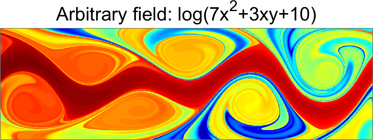
(a)

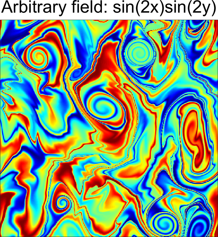
(b)

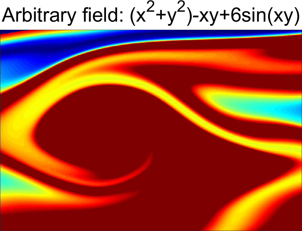
(c)

Figure 1: Three arbitrary advected scalar fields evaluated on advected particle positions $(x,y)$ at the end time, then plotted over the initial positions $(x_{0},y_{0})$ of the particles. (a) quasiperiodic Bickley jet (b) two-dimensional turbulence (c) observed wind field of Jupiter.

These three examples include the following:

1. The Bickley jet: an analytically defined velocity field with quasi-periodic time dependence.

2. Two-dimensional turbulence: a high-resolution data set obtained from the direct numerical simulation of the Navier–Stokes equations in two dimensions.

3. Jupiter’s wind field: an observational data set of Jupiter’s atmospheric velocities, reconstructed from video footage taken by the Cassini spacecraft..

These examples are ordered in an increasing level of difficulty, given how much information is available about the flow in each of them. The Bickley jet velocity field is temporally aperiodic but recurrent, and known analytically at all locations and times. The two-dimensional turbulence data set is slightly more challenging, as the velocity field is fully aperiodic, known only at discrete points in space and time. One could, however, still increase the resolution of the data by solving the Navier–Stokes equations over finer grids (or, equivalently, by including more Fourier modes). Furthermore, the temporal duration of the data set can also be increased at will. The third example involving the Jupiter’s atmospheric velocities poses the greatest challenge, as the spatial and temporal length and resolution of this fully aperiodic data set is limited by the available video footage recorded by the Cassini mission.

Comparisons of a limited number of methods on specific structures in individual examples have already appeared Beron-Vera et al. (2013); Haller et al. (2016); Ma and Bollt (2015). Here the objective is to perform a systematic comparison on a variety of challenging flow fields in which a ground truth can nevertheless be reasonably established. Our scope is also broader in that we cover all known types of Lagrangian structures in two-dimensions: elliptic (vortex-type), hyperbolic (repelling or attracting) and parabolic (jet-core-type) material structures.

The rest of this paper is organized as follows. In Sections II, III and IV, we introduce the twelve diagnostic and analytic methods considered in this comparison. Despite our efforts to keep the method descriptions to a minimum, the introduction of analytic methods necessarily takes up more space due to the need to explain the mathematical principles underlying them. In Section V, the methods are applied to the three examples, with different aspects of their performance compared. Our overall assessment of the strengths and weaknesses of each method appears in Section VI, and a proposed set of minimal requirements for Lagrangian coherence detection methods is given in Section VII.

II General setup

We consider here flows defined by two-dimensional unsteady velocity fields $v(x,t)$ known over a finite time interval $[t_{0},t_{1}]$. The fluid particle motions satisfy the differential equation

$$\dot{x}=v(x,t),\quad x\in U\subset\mathbb{R}^{2},\quad t\in[t_{0},t_{1}],$$ (1)

whose trajectories are denoted by $x(t;t_{0},x_{0})$, with $x_{0}$ referring to their initial position at time $t_{0}$. Our focus here is Lagrangian, concerned with coherent behavior exhibited by sets of trajectories of (1). This is in contrast to the classic Eulerian approach taken in fluid mechanics which focuses on coherent features of $v(x,t)$.

Central to all Lagrangian approaches is the flow map

$$F_{t_{0}}^{t}(x_{0}):x_{0}\mapsto x(t;t_{0},x_{0}),$$ (2)

mapping initial positions $x_{0}$ to their current positions $x$ at time $t$. Several Lagrangian coherence-detection methods also rely on the flow gradient $\nabla F(x_{0})$ (or deformation gradient), the derivative of the flow map with respect to the initial condition $x_{0}$. The stretching induced by the flow gradient is captured by the right Cauchy–Green strain tensor $C_{t_{0}}^{t}$ of the deformation field, defined as Truesdell and Noll (2004)

$$C_{t_{0}}^{t}(x_{0})=\left[\nabla F_{t_{0}}^{t}\right]^{\intercal}\nabla F_{t_{0}}^{t},$$ (3)

with the symbol $\intercal$ indicating matrix transposition. In our present two-dimensional setting, the symmetric and positive definite tensor $C_{t_{0}}^{t}$ has two positive eigenvalues $0<\lambda_{1}\leq\lambda_{2}$ and an orthonormal eigenbasis $\left\{\xi_{1},\xi_{2}\right\}$ satisfying

$$C_{t_{0}}^{t}(x_{0})\xi_{i}(x_{0})=\lambda_{i}(x_{0})\mathbf{\xi}_{i}(x_{0}),\quad\left|\xi_{i}(x_{0})\right|=1,\quad i=1,2,$$

$$\xi_{2}(x_{0})=\Omega\xi_{1}(x_{0}),\quad\Omega=\left(\begin{array}[]{cc}0&-1\\ 1&0\end{array}\right).$$ (6)

III Diagnostics for Lagrangian coherence

We first briefly review five Lagrangian diagnostic scalar fields that have been proposed for material coherence detection in the literature. They are classified as Lagrangian because their pointwise value at a point $x_{0}$ of the flow domain depends solely on the trajectory segment running from the location $x_{0}$ at time $t_{0}$ up to the location $F_{t_{0}}^{t_{1}}(x_{0})$ at time $t_{1}$. Based on simple geometric or physical arguments, these diagnostics are expected to highlight coherence or lack thereof in the flow. Most of them, however, offer neither a strict definition of the coherent flow structures they seek, nor a precise mathematical connection between their geometric features and those flow structures.

A basic expectation for such diagnostic scalar fields is that they should at least outperform generic passively advected scalar fields in their diagnostic abilities. By definition, Lagrangian coherent structures (LCSs) create coherent trajectory patterns Haller (2015), and hence the footprint of LCSs should invariably appear in any generic tracer distribution advected by trajectories. To this end, in our comparisons performed on given examples, we have also included ad hoc passive scalar fields as baselines for the efficacy of diagnostic and mathematical approaches (see Figure 1).

Another expectation for Lagrangian diagnostics stems from the fact that LCSs are composed of the same material trajectories, irrespective of what coordinate system we use to study them. Therefore, the assessment of whether or not a trajectory is part of an LCS is inherently independent of the frame of the observerPeacock, Froyland, and Haller (2015). Any self-consistent two-dimensional LCS method should, therefore, identify the same set of trajectories as LCSs under all Euclidean observer changes of the form $x=Q(t)y+b(t),$ where $y\in\mathbb{R}^{2}$ is the coordinate in the new frame, $Q(t)\in SO(2)$ represents time-dependent rotation, and $b(t)\in\mathbb{R}^{2}$ represents time-dependent translation. A similar requirement holds, with appropriate modifications, for three-dimensional LCS-detection methods.

Frame-invariance is particularly important in truly unsteady flows, which have no distinguished frame of reference Lugt (1979). Within this class, geophysical fluid flows represent an additional challenge, because they are defined in a rotating frame. The detection or omission of a feature by a diagnostic in such flows, therefore, should clearly not be an artifact of the co-rotation of the frame with the Earth. For each surveyed diagnostic below, we will discuss its objectivity or lack thereof.

III.1 Finite-time Lyapunov exponent (FTLE)

Haller Haller and Yuan (2000); Haller (2002) proposed that the time $t_{0}$ positions of the strongest repelling LCSs over the time interval $[t_{0},t_{1}]$ should form ridges of the finite-time Lyapunov exponent (FTLE) field

$$\begin{split}\text{FTLE}_{t_{0}}^{t_{1}}(x_{0})&=\frac{1}{\left|t_{1}-t_{0}\right|}\log\left\|\nabla F_{t_{0}}^{t_{1}}(x_{0})\right\|\\ &=\frac{1}{\left|t_{1}-t_{0}\right|}\log\sqrt{\lambda_{2}(x_{0})}.\end{split}$$ (7)

Similarly, time $t_{1}$ positions of the strongest attracting LCSs over $[t_{0},t_{1}]$ are expected to be marked by ridges of the backward-time FTLE field $\text{FTLE}_{t_{1}}^{t_{0}}$. Repelling and attracting LCSs are usually referred to as hyperbolic LCSs, as they generalize the notion of hyperbolic invariant manifolds to finite-time dynamics. The FTLE field is objective by the objectivity of the invariants of the Cauchy–Green strain tensor Gurtin (1982).

The FTLE field (7) measures the largest finite-time growth exponent experienced by infinitesimal perturbations to the initial condition $x_{0}$ over the time interval $[t_{0},t_{1}]$. It is therefore a priori unclear if a given FTLE ridge indeed marks a repelling material surface, or just a surface of high shear (cf. Ref. Haller, 2015 for an example). Nevertheless, time-evolving FTLE ridges computed over sliding intervals $[t_{0}+T,t_{1}+T]$ with varying $T$ are often informally identified with LCSs. There are, however, both conceptual and mathematical issues with such an identification, and the evolving ridges so obtained may be far from Lagrangian Haller (2015).

Motivated by the fact that material stretching is minimal along jet steams, FTLE trenches have been proposed for detection of unsteady jet cores (or parabolic LCSs)Beron-Vera et al. (2010, 2012). While, in many examples, the jet cores are closely approximated by the FTLE trenches, there exist counterexamples where an FTLE trench does not coincide with the jet Farazmand, Blazevski, and Haller (2014).

The FTLE diagnostic is not geared towards detecting elliptic (vortex-type) LCSs in finite-time flow data. While the FTLE values are expected to be low near elliptic LCS, a sharp boundary for vortex-type structures does not generally emerge from this diagnostic, as seen in our examples below.

III.2 Finite-Size Lyapunov Exponent (FSLE)

An alternative assessment of perturbation growth in the flow is provided by the Finite-Size Lyapunov exponent (FSLE). To define this quantity, we first select an initial separation $\delta_{0}>0$ and a separation factor $r>1$ of interest. The separation time $\tau(x_{0};\delta_{0},r)$ is then defined as the minimal time in which the distance between a trajectory starting from $x_{0}$ and some neighboring trajectory starting $\delta_{0}$-close to $x_{0}$ first reaches $r\delta_{0}$. The FSLE associated with the location $x_{0}$ is then defined as Artale et al. (1997); Aurell et al. (1997); Joseph and Legras (2002)

$$\text{FSLE}(x_{0};\delta_{0},r)=\frac{\log r}{\tau(x_{0};\delta_{0},r)}.$$ (8)

In contrast to the FTLE field, the FSLE field focuses on separation scales exceeding the threshold $r$, and hence can be used for selective structure detection. A further conceptual advantage of the FSLE field is that its computation requires no a priori choice of an end time $t_{1}$.

By analogy with FTLE ridges, FSLE ridges have also been proposed as indicators of hyperbolic LCSs (see Refs. Joseph and Legras, 2002; d’Ovidio et al., 2004; Bettencourt, López, and Hernández-García, 2013). This analogy is mathematically justified for sharp enough FSLE ridges of nearly constant height Karrasch and Haller (2013). A general correspondence between FSLE and FTLE ridges, however, does not exist. This is because $\text{FSLE}(x_{0};\delta_{0},r)$ lumps trajectory separation events occurring over different time intervals into the same scalar field, and hence has no general relationship to the single finite-time flow map $F_{t_{0}}^{t}(x_{0})$.

The FSLE field has generic jump discontinuities and a related sensitivity to the computational time step (see Ref. Karrasch and Haller, 2013 for details). The FSLE, however, is still an objective field, given that it is purely a function of particle separation.

III.3 Mesochronic analysis

Mezić et al. Mezić et al. (2010) proposed the eigenvalue configuration of the deformation gradient $\nabla F_{t_{0}}^{t_{1}}(x_{0})$ as a diagnostic for qualitatively different regions of material mixing. Specifically, their mesochronic classification considers regions where $\nabla F_{t_{0}}^{t_{1}}(x_{0})$ have real eigenvalues as mesohyperbolic, and regions where $\nabla F_{t_{0}}^{t_{1}}(x_{0})$ has complex eigenvalues as mesoelliptic. Mesohyperbolic regions are further divided into two categories as follows. Since $\nabla F_{t_{0}}^{t_{1}}(x_{0})$ is an orientation preserving diffeomorphism, we necessarily have $\det\nabla F_{t_{0}}^{t_{1}}(x_{0})>0$, which implies that real eigenvalues of $\nabla F_{t_{0}}^{t_{1}}(x_{0})$ are either both negative or both positive. Mezic et al. Mezić et al. (2010) refer to the case where the real eigenvalues are both positive as mesohyperbolic without (a $180^{\circ}$) rotation. If the eigenvalues are real and negative, the trajectory is called mesohyperbolic with (a $180^{\circ}$) rotation.

Data collected in the aftermath of Deepwater Horizon Spill Mezić et al. (2010) shows that mixing zones in the ocean are predominantly mesohyperbolic when the integration time is selected to be about 4 days. Longer studies of ocean data suggest that oceanic flows are predominantly mesoelliptic over time scales beyond four days Beron-Vera et al. (2013). This is in line with the expectation that accumulated material rotation along general trajectories unavoidably creates nonzero imaginary parts for the eigenvalues of $\nabla F_{t_{0}}^{t_{1}}(x_{0})$, even if the underlying trajectory starting from $x_{0}$ is of saddle-type.

From a mathematical point of view, the linear mapping $\nabla F_{t_{0}}^{t_{1}}(x_{0})$ is a two-point-tensor between the tangent spaces $T_{x_{0}}\mathbb{R}^{2}$ and $T_{F_{t_{0}}^{t_{1}}(x_{0})}\mathbb{R}^{2}$ of $\mathbb{R}^{2}$. Posing an eigenvalue problem for $\nabla F_{t_{0}}^{t_{1}}(x_{0})$ is, therefore, only meaningful when these tangent spaces coincide, i.e., $x_{0}=F_{t_{0}}^{t_{1}}(x_{0})$ lies on a trajectory that returns exactly to its starting point at time $t$. For this reason, it is difficult to attach a mathematical meaning to the mesochronic partition in general unsteady flows in which such returning trajectories are nonexistent.

The mesochronic partition of the flow domain is not objective due to the frame-dependence of the deformation gradient $\nabla F_{t_{0}}^{t_{1}}(x_{0})$ (see e.g., Ref. Liu, 2003). As a consequence, the elliptic-hyperbolic classification of trajectories obtained from this method will change under changes of the observer.

The mesochronic notions of hyperbolicity and ellipticity differ from classic hyperbolicity and ellipticity concepts for Lagrangian trajectories. Even regions of concentric closed orbits in a steady flow (a classic case of elliptic particle motion) are marked by nested sequences of alternating mesoelliptic and mesohyperbolic annuli (see Ref. Mezić et al., 2010 for an example). No published account of a coherent vortex definition from these plots is yet available, but outermost boundaries of smooth and nested elliptic, hyperbolic-with-rotation annulus sequences have recently been suggested as coherent structure boundaries Mezić (2015) for general unsteady flow. We will adopt this definition (i.e., at least three nested annuli of different mesochronic types, containing no saddle-type critical points of $\det\nabla F_{t_{0}}^{t_{1}}(x_{0})$) for a mesoelliptic coherent structure in our comparison study.

III.4 Trajectory length

Mancho et al. Mancho et al. (2013) propose that abrupt variations (i.e., curves of high gradients) in the arc-length function

$$M_{t_{0}}^{t_{1}}(x_{0})=\int_{t_{0}}^{t_{1}}\left|v(x(s;t_{0},x_{0}),s)\right|ds$$

of the trajectory $x(s;t_{0},x_{0})$ indicate the time $t_{0}$ positions of boundaries of qualitatively different dynamics. The $M_{t_{0}}^{t_{1}}(x_{0})$ function is arguably the quickest to compute of all Lagrangian diagnostics considered here. It also naturally lends itself to applications to float data, given that the arclength of a trajectory can be computed without any reliance on a velocity field or on neighboring trajectories.

As any scalar field computed along trajectories, $M_{t_{0}}^{t_{1}}(x_{0})$ is generally expected to show an imprint of Lagrangian coherent structures, as indeed found by Mancho et al. Mancho et al. (2013). There is, however, no established mathematical connection between material coherent structures and features of $M_{t_{0}}^{t_{1}}(x_{0})$. Indeed, several counter-examples to coherent structure detection based on trajectory length are available.Ruiz-Herrera (2015, 2016).

The function $M_{t_{0}}^{t_{1}}(x_{0})$ is not objective or even Galilean invariant. For instance, in a frame co-moving with any selected trajectory $x(s;t_{0},x_{0})$, the trajectory itself has zero arclength, and hence its initial condition $x_{0}$ will generically be a global minimum. The level curve structure of $M_{t_{0}}^{t_{1}}(x_{0})$ is not objective either, because the integrand of its gradient field $\nabla M_{t_{0}}^{t_{1}}(x_{0})$ consists of elements that are frame-dependent.

III.5 Trajectory complexity

Rypina et al. Rypina et al. (2011) propose a partitioning of the flow domain into regions where trajectories exhibit different levels of complexity. They quantify individual trajectory complexity over a finite time interval $[t_{0},t_{1}]$ using the ergodicity defect (cf. Ref. Scott et al., 2009)

$$d(s;x_{0},t_{0})=\sum\limits_{j=1}^{K}\,\,\left[\frac{N_{j}(s)}{N}-s^{2}\right]^{2},f$$ (9)

where $N$ is the total number of trajectories, and $N_{j}(s)$ is the the number of trajectory points that lie inside the $j^{th}$ element of a square grid of side-length $s$. The integer $K=1/s^{2}$ denotes the total number of boxes forming the grid. The total area of the full flow domain is normalized to unity. Mathematically, formula (9) is just the $L^{2}$ deviation of a histogram based on the trajectory points from a constant histogram.

The “most non-ergodic trajectory” is a fixed point, for which we obtain $d=1$. In contrast, for an “ergodic trajectory” (uniformly distributed trajectory), one should obtain $\lim_{s\to 0}d(s;x_{0},t_{0})=0$. Rypina et al. Rypina et al. (2011) define the average ergodicity defect over different scales of $s$ as

$$\bar{d}(s;x_{0},t_{0})=\mathrm{mean}_{s}(d(s;x_{0},t_{0})),$$ (10)

where the mean is taken over a broad range of spatial scales $s$ of interest.

While no mathematical connection is known between the ergodicity defect and finite-time coherent structures, locations of abrupt changes (large gradients) in the topology of $\bar{d}(s;x_{0},t_{0})$ as a function of $x_{0}$ are expected to mark boundaries between qualitatively different flow regions. The quantity $\bar{d}(s;x_{0},t_{0})$ is objective, because presence in, or absence from, a grid cell is invariant under rotations and translations, as long as the same rotations and translations are applied to both the trajectories and the grid cells. The approach is simple to implement and has proven itself effective on low-resolution data Rypina et al. (2011).

III.6 Shape coherence

Ma and Bollt Ma and Bollt (2014) seek coherent set boundaries as closed material lines at time $t_{0}$ that are nearly congruent with their advected images at time $t_{1}$. Such near-congruence is ensured by classic results if the curvature distributions along the original and advected curve are close enough.

Motivated by examples of steady linear flows, Ma and Bollt Ma and Bollt (2014) propose finding shape-coherent curves as minimizers of the angle between the dominant eigenvectors of the forward-time and the backward-time Cauchy–Green strain tensors. Stated in our present context, the position of the boundary of a shape-coherent set at time $\hat{t}=(t_{0}+t_{1})/2$ is a closed curve along which the splitting angle function

$$\theta(\hat{x}_{0})=\arcsin\left(|\xi_{2}^{fw}(\hat{x}_{0})\times\xi_{2}^{bw}(\hat{x}_{0})|\right),\qquad\hat{x}_{0}=F_{t_{0}}^{\hat{t}}(x_{0}),$$ (11)

vanishes. Here we used the definitions

$$C_{\hat{t}}^{t_{1}}(\hat{x}_{0})\xi_{2}^{fw}(\hat{x}_{0})=\lambda_{2}^{fw}(\hat{x}_{0})\xi_{2}^{fw}(\hat{x}_{0}),\qquad C_{\hat{t}}^{t_{0}}(\hat{x}_{0})\xi_{2}^{bw}(\hat{x}_{0})=\lambda_{2}^{bw}(\hat{x}_{0})\xi_{2}^{bw}(\hat{x}_{0}),\qquad\left|\xi_{2}^{fw}\right|=\left|\xi_{2}^{bw}\right|=1.$$

Ma and Bollt Ma and Bollt (2014, 2015) argue that level curves of eq. (11) with $\left|\theta(\hat{x}_{0})\right|\ll 1$ should show significant shape coherence over a finite time interval. They support this expectation with examples of steady, linear velocity fields.

For unsteady flows with general time dependence, the smallness of $\left|\theta(\hat{x}_{0})\right|\ll 1$ along closed structure boundaries remains a heuristic assertion that we will test here on temporally aperiodic examples. Locating closed level curves of $\theta(\hat{x}_{0})$ reliably is a highly challenging numerical problem to which Refs. Ma and Bollt, 2014, 2015 offer no immediate solution. For a direct comparison with other methods, we will simply identify the set $\left|\theta(\hat{x}_{0})\right|\ll 1$ for initial conditions $\hat{x}_{0}$ seeded at time $\hat{t}$, then advect these initial conditions under the flow map $F_{\hat{t}}^{t_{0}}$ to time $t_{0}$. The resulting open set must then necessarily contain the structure boundary curves envisioned by Refs. Ma and Bollt, 2014, 2015. The splitting angle diagnostic (11) is objective, given that it only depends on the angle between appropriate Cauchy–Green eigenvectors.

IV Mathematical approaches to Lagrangian coherence

Here we recall approaches that locate coherent structures by providing precise solutions to mathematically formulated coherence principles. These approaches, however, are only precise relative to their starting coherence principle. One still needs to test whether those coherence principles capture observed coherent trajectory patterns consistently and effectively in various finite-time data sets. Indeed, a heuristic but well-motivated diagnostic tool may consistently outperform a rigorous mathematical approach that is based on an ineffective coherence principle.

As in the case of diagnostics, we consider frame-indifference (or objectivity) to be a fundamental requirement for the self-consistency of mathematical approaches to Lagrangian coherence. All mathematical approaches considered below satisfy this requirement.

IV.1 Transfer operator method

Transfer operator approaches provide a global view of density evolution in the phase space, identifying maximally coherent or minimally dispersive regions over a finite time interval $[t_{0},t_{1}]$. Such regions are known as almost-invariant sets for autonomous systems Dellnitz and Junge (1999); Froyland (2005); Froyland and Padberg (2009) or coherent sets for non-autonomous systems Froyland, Lloyd, and Santitissadeekorn (2010); Froyland, Santitissadeekorn, and Monahan (2010); Froyland (2013) and minimally mix with the surrounding phase space.

IV.1.1 Probabilistic transfer operator method

Following the approach from Ref. Froyland, 2013, we let $M\subset\mathbb{R}^{d}$ be a compact domain and let $\mu$ denote a reference probability measure on $M$ representing the distribution or concentration of a quantity of interest. In many cases, one would select $\mu$ to be the normalized volume on $M$; this would treat all parts of the phase space equally. In other cases, one might select $\mu$ to be the distribution of a chemical in a fluid or the distribution of a (compressible) air mass in the atmosphere.

We now imagine advection-diffusion dynamics; this could arise from purely advective dynamics with some additional small amplitude $\epsilon$-diffusion, as in the examples considered in this comparative study, or this could be genuine advection-diffusion dynamics. Specializing to the former case, we have a flow map $F_{t_{0}}^{t_{1}}:M\to F_{t_{0}}^{t_{1}}(M)$ from some initial time $t_{0}$ to some final time $t_{1}$. Roughly speaking, we wish to identify subsets $A_{t_{0}}\subset M$, $A_{t_{1}}\subset F_{t_{0}}^{t_{1}}(M)$ that maximize the quantity

$$\mu(A_{t_{0}}\cap(F_{t_{0}}^{t_{1}})^{-1}A_{t_{1}})/\mu(A_{t_{0}}),$$

subject $\mu(A_{t_{0}})\leq 1/2$ ($A_{t_{0}}$ comprises not more than half of $M$). The numerator represents the $\mu$-proportion of $A_{t_{0}}$ that is mapped into $A_{t_{1}}$, and the entire expression is therefore the fraction of $\mu$-mass that is mapped from $A_{t_{0}}$ to $A_{t_{1}}$.

The determination of these sets is achieved by computing the second singular value of a normalized transfer operator $\cal{L}_{\epsilon}$ and extracting the sets $A_{t_{0}}$ and $A_{t_{1}}$ from level sets of the corresponding left and right singular vectors, respectively; see Ref. Froyland, 2013 or the survey Ref. Froyland and Padberg-Gehle, 2014 for details.

One can characterise the amount of mixing that has occurred during the interval $[t_{0},t_{1}]$ as

$$\rho:=\max_{A_{t_{0}},A_{t_{1}}\subset M}\left\{\frac{\langle\mathcal{L}_{\epsilon}\mathbf{1}_{A_{t_{0}}},\mathbf{1}_{A_{t_{1}}}\rangle}{\mu(A_{t_{0}})}+\frac{\langle\mathcal{L}_{\epsilon}\mathbf{1}_{A_{t_{0}}^{c}},\mathbf{1}_{A_{t_{1}^{c}}}\rangle}{\mu(A_{t_{0}^{c}})}\right\}.$$ (12)

The quantity $\rho$ probabilistically quantifies the degree to which one can find agreement between pairs of sets $F^{t_{1}}_{t_{0}}A_{t_{0}}$ and $A_{t_{1}}$ (and between their complements). Larger $\rho$ means sets can be found with greater agreement and that less mixing has occurred. One has the theoretical upper bound $\rho\leq 1+\sigma_{2}$, where $\sigma_{2}$ is the second singular value of $\mathcal{L}_{\epsilon}$ (Theorem 2 [48]). One can represent (12) as an $L^{2}$ maximisation problem, the solutions of which are left and right singular vectors of $\mathcal{L}_{\epsilon}$; see [48]. The objective of this maximisation problem is an $L^{2}$ relaxation of (12) and using a standard approach, one recovers feasible solutions of (12) as optimal level sets (optimal according to the objective (12)) of the solutions of the relaxation; in this case, level sets of the left and right singular vectors. Further singular vectors can be used to find multiple coherent sets by either (i) thresholding individual singular vectors as in the numerics section, or (ii) clustering several vectors embedded in Euclidean space as in Ref. Froyland, 2005.

In practice, a common way to numerically compute $\mathcal{L}$ is to use Ulam’s method. One (i) partitions $M$ and $F_{t_{0}}^{t_{1}}(M)$ into a fine grid of sets, (ii) samples several initial points in each grid set, (iii) numerically integrates these initial points, and (iv) computes grid set to grid set transition probabilities by counting how many initial points from each grid set $A$ enter another grid set $B$. If there are $m$ grid sets in $M$ and $n$ grid sets in $F_{t_{0}}^{t_{1}}(M)$, one obtains a sparse $m\times n$ stochastic transition matrix $P$, which may be identified as a Markov chain transition matrix with each grid set considered a state. One now normalizes this matrix $P$ to produce a matrix $L$ approximating $\mathcal{L}$ and computes singular vectors (see Refs. Froyland, Santitissadeekorn, and Monahan, 2010; Froyland, 2013 for details). The small additional $\epsilon$-diffusion need not be explicitly simulated because numerical diffusion already arises from the discretization of $M$ and $F_{t_{0}}^{t_{1}}(M)$ into grid sets.

Alternative, non-Ulam numerical implementations of variations of the transfer operator method from Ref. Froyland, 2013 include Ref. Williams, Rypina, and Rowley, 2015 which uses approximate Galerkin projection onto a basis of thin-plate splines; Ref. Denner, Junge, and Matthes, 2015 which uses spectral collocation, and Ref. Banisch and Koltai, 2016, which uses diffusion map constructions.

IV.1.2 Dynamic Laplace operator method

Considering the $\epsilon\to 0$ (i.e., zero diffusion amplitude) limit in the previous section leads to a geometric theory of finite-time coherent sets, which targets the boundaries of coherent families of sets. For simplicity of presentation, assume that the flow map $F_{t_{0}}^{t_{1}}:M\to F_{t_{0}}^{t_{1}}(M)$ from the previous section is volume-preserving. The goal of the dynamic Laplacian approach Froyland (2015) is to seek surfaces $\Gamma\subset M$ that disconnect a bounded phase space $M$ in such a way that the advected disconnecting surface $F_{t_{0}}^{t_{1}}(\Gamma)$ remains as short as possible relative to the volume of the disconnected parts for $t\in[t_{0},t_{1}]$. Thus, the region enclosed by $\Gamma$ (or by $\Gamma$ and by the boundary of the phase space) is coherent because filamentation of the boundary is minimized under nonlinear evolution of the dynamics. Specifically, for a finite subset $\mathcal{T}$ of $[t_{0},t_{1}]$ containing $t_{0}$ and $t_{1}$, the quantity $(\frac{1}{|\mathcal{T}|}\sum_{t\in\mathcal{T}}\ell_{d-1}(F_{t_{0}}^{t}(\Gamma)))/\min\{\ell(M_{1}),\ell(M_{2})\}$ is minimized over smooth disconnecting $\Gamma$, where $\ell$ is the volume measure on the phase space, $\ell_{d-1}$ is the induced volume measure for hypersurfaces, and $M_{1},M_{2}$ partition phase space with shared smooth boundary $\Gamma$.

To solve this problem, one considers the dynamic Laplace operator

$$\triangle^{D}:=\frac{1}{|\mathcal{T}|}\sum_{t\in\mathcal{T}}F_{t_{0}}^{t}\circ\triangle\circ(F_{t_{0}}^{t})^{-1}$$

on $M$. The standard Laplace-Beltrami operator $\triangle$ is extensively used in manifold learning or nonlinear dimensionality reduction via Laplace eigenmaps and spectral clustering Belkin and Niyogi (2003). The second and lower eigenvectors of $\triangle^{D}$ reveal further geometric information in analogy to the eigenvectors of the standard (static) Laplace operator Belkin and Niyogi (2003) and multiple coherent sets can be extracted using the methods described in the previous section for transfer operators. In practice, one approximates the above operator with a numerical method appropriate for elliptic self-adjoint operators (e.g. finite difference Froyland (2015), radial basis function collocation Froyland and Junge (2015), or others).

Because this method arises as a zero-diffusion limit Froyland (2015) of the probabilistic transfer operator method discussed in the previous section, the numerical results obtained from the dynamic Laplace operator approach are very similar and will not be discussed separately in our comparison. Both the probabilistic transfer operator and dynamic Laplace operator methods are objective by construction. An advantage of the dynamic Laplace operator approach is the flexibility in the method of approximation of the operators. Higher-order schemes may be employed when the dynamics is smooth in order to exploit the smoothness and reduce the input and computational requirements Froyland and Junge (2015). The theory and constructions for general non-volume-preserving $F_{t_{0}}^{t_{1}}$ and general reference measure $\mu$ are developed in Ref. Froyland and Kwok, 2016. Ref. Karrasch and Keller, 2016 describes a related theory based on a single Riemannian metric.

IV.2 Hierarchical coherent pairs

The transfer operator method described in Ref. Froyland, Santitissadeekorn, and Monahan, 2010 focused primarily on identifying two sets, $A_{0}$ and its complement $\widetilde{A}_{0}$, that partition a given region of interest into two coherent sets. Ma and Bollt MA and BOLLT (2013) propose an extension of this idea that enables the identification of multiple coherent pairs in a given domain. The extension is based on an iterative and hierarchical refinement of coherent pairs using a reference measure of probability $\mu$. Specifically, Ma and Bollt MA and BOLLT (2013) refine the coherent pairs $A_{0}$ and $\widetilde{A}_{0}$ identified earlier over several steps by applying the probabilistic transfer operator method restricted to these sets. This iterative refinement of coherent pairs can be stopped once $\mu$ shows no appreciable improvement compared to the earlier iterations. We refer to this method as hierarchical transfer operator method throughout our comparison. This “repeated bisection” approach is an alternative to extracting multiple coherent sets using multiple singular vectors of $\mathcal{L}$ as described in the previous section.

IV.3 Fuzzy cluster analysis of trajectories

Recently, Froyland and Padberg-Gehle Froyland and Padberg-Gehle (2015) proposed a method based on traditional fuzzy C-means clustering Bezdek (1981); Dunn (1973) to identify finite-time coherent regions from incomplete and sparse trajectory data set. Their method locates coherent sets as clusters of trajectories according to the dynamic distance $D(x,y)=\int_{t_{0}}^{t_{1}}\|x(t)-y(t)\|^{2}\ dt$, where $x(t),y(t)$ are a pair of trajectories over a finite time interval $[t_{0},t_{1}]$.

To identify such coherent sets, Ref. Froyland and Padberg-Gehle, 2015 first constructs a trajectory array $X\in\mathbb{R}^{n\times dm}$ whose rows are vectors $(X_{i})_{i=1,\ldots,n}$ containing concatenated positions of $n$ Lagrangian particles over $m$ discrete time intervals in $d$-dimensional space; that is, $x_{i}=(x_{i,t_{0}},\ldots,x_{i,t_{1}})$. Second, Ref. Froyland and Padberg-Gehle, 2015 applies the fuzzy C-means (FCM) algorithm to the trajectory array $X$, which seeks to split the trajectories into $K$ clusters based on the distance between a given trajectory point $X_{i}$ and initial cluster centers $(C_{j})_{j=1,\ldots,K}$ predefined in $\mathbb{R}^{dm}$, using the following objective function:

$$\min\sum_{i=1}^{n}\sum_{j=1}^{c}u_{ij}^{m}\left\|X_{i}-C_{j}\right\|^{2}=\min u_{ij}^{m}\sum_{t=t_{0}}^{t_{1}}\|x_{i,t}-c_{j,t}\|^{2},$$ (13)

where $u_{i,j}$ is the membership value defined as

$$u_{i,j}=\left[\sum\limits_{j=1}^{K}\left(\frac{\|X_{i}-C_{k}\|}{\|X_{i}-C_{j}\|}\right)^{\frac{2}{m-1}}\right]^{-1},\qquad 0\leq u_{i,j}\leq 1,\qquad 1\leq m<\infty.$$ (14)

The membership value $u_{i,j}$ describes the likelihood that a trajectory point $X_{i}$ belongs to a cluster associated with the cluster center $C_{j}$, for a fixed parameter $m$ specified in advance.

The parameter $m$ determines the fuzziness of cluster boundaries, that is how much clusters are allowed to overlap. A large $m$ results in less extreme membership values $u_{k,j}$, and consequently fuzzier clusters. In the limit $m=1$, the memberships converge to $0$ or $1$, and hence the FCM results in non-overlapping clusters in a fashion similar to the K-means algorithm Lloyd (2006). The cluster center is the mean of all trajectory points, weighted by the degree of belonging to each of the $K$ clusters. Specifically, the $j^{th}$ cluster center is defined as

$$C_{j}=\frac{\sum\limits_{i=1}^{n}\left(u_{i,j}\right)^{m}X_{i}}{\sum\limits_{i=1}^{n}\left(u_{i,j}\right)^{m}}.$$ (15)

To optimize (13), the FCM algorithm iteratively computes membership values (14) and relocates the cluster centers using (15), until the objective function (13) shows no substantial improvement. Finally, given the membership values $u_{i,j}$ and cluster centers $C_{j}$, each trajectory is assigned to only one cluster based on the maximum membership value it carries.

Those trajectories carrying low membership values for all clusters, with respect to a given threshold (selected as $0.9$ in all our examples below), are occasionally considered to be non-coherent Froyland and Padberg-Gehle (2015). The incomplete data case (e.g., some or all trajectories have missing “gaps”) is also described in Ref. Froyland and Padberg-Gehle, 2015. We finally note that the fuzzy cluster analysis of trajectories is an objective approach, as the label of trajectories remains invariant under any affine coordinate transformation Froyland and Padberg-Gehle (2015).

IV.4 Spectral clustering of trajectories

Hadjighasem et al. Hadjighasem et al. (2016) propose spectral clustering to identify coherent structures by grouping Lagrangian particles into coherent and incoherent clusters. Specifically, they define a coherent structure as a distinguished set of Lagrangian trajectories that maintain short distances among themselves relative to their distances to trajectories outside the structure.

The spectral clustering approach starts with $n$ trajectories whose positions are available at $m$ discrete times $t_{0}<t_{1}<\ldots<t_{k}<\ldots<t_{m-1}=t_{f}$ in a two-dimensional spatial domain. This information is stored in an $n\times m\times 2$-dimensional numerical array with elements $\mathbf{x}_{k}^{i}\coloneqq\mathbf{x}^{i}(t_{k})\in\mathbb{R}^{2}$. The dynamical distance $r_{ij}$ between Lagrangian particles $\mathbf{x}^{i}$ and $\mathbf{x}^{j}$ is then defined as

$$\begin{split}r_{ij}&\coloneqq\frac{1}{t_{f}-t_{0}}\int_{t_{0}}^{t_{f}}\left|\mathbf{x}^{i}(t)-\mathbf{x}^{j}(t)\right|\mathrm{d}t\\ &\approx\frac{1}{t_{f}-t_{0}}\sum_{k=0}^{m-2}\frac{t_{k+1}-t_{k}}{2}\left(\left|\mathbf{x}_{k+1}^{i}-\mathbf{x}_{k+1}^{j}\right|+\left|\mathbf{x}_{k}^{i}-\mathbf{x}_{k}^{j}\right|\right),\end{split}$$ (16)

where $\left|\cdot\right|$ denotes the spatial Euclidean norm. Note that the dynamic distance (16) is an objective metric, as it only depends on the distance of trajectory points.

Next, Ref. Hadjighasem et al., 2016 constructs a similarity graph $G=(V,E,W)$, which is specified by the set of its nodes $V={v_{1},\ldots,v_{N}}$, the set of edges $E\subseteq V\times V$ between nodes, and a symmetric similarity matrix $W\in\mathbb{R}^{n\times n}$ which assigns weights $w_{ij}$ to the edges $e_{ij}$. The similarity matrix entries (or weights) $w_{ij}\geq 0$ give the probability of nodes $v_{i}$ and $v_{j}$ to be in the same cluster. In the context of coherent structure detection, the graph nodes $V$ are Lagrangian particles themselves, with the associated similarity weights defined as

$$w_{ij}=1/r_{ij}\quad\text{for}\;i\neq j.$$ (17)

With the similarity weights at hand, the degree of a node $v_{i}\in V$ is defined as

$$\text{deg}(v_{i})\coloneqq\sum_{j=1}^{n}w_{ij}.$$

The subsequent degree matrix $D$ is then constructed as a diagonal matrix with the degrees $\deg(v_{i})$ in the diagonal. Given a subset of nodes $A\in V$, the size of $A$ is measured by

$$\operatorname{vol}(A)\coloneqq\sum_{i\in A}\deg(v_{i}),$$

with summation over the weights of all edges attached to nodes in $A$.

With the notation developed so far, the problem of coherent structure detection can now be posed in terms of a normalized graph cut problem: Given a similarity graph $G=(V,E,W)$, partition the graph nodes $V$ into $k$ sets $A_{1},A_{2},\ldots,A_{k}$ such that the following conditions hold:

Within-cluster similarity

Nodes in the same cluster are similar to each other, i.e., particles in a coherent structure have mutually short dynamical distances.

Between-cluster dissimilarity

Nodes in a cluster are dissimilar to those located in the complementary cluster. In other words, particles in a coherent structure have long dynamical distances from the rest of the particles, particularity from those located in the mixing region (i.e., noise cluster) that fills the space outside the coherent structures.

The normalized cut that implements the above (dis)similarity conditions can be formulated mathematically as

$$\operatorname{NCut}(A_{i},...,A_{k})=\frac{1}{2}\sum_{i=1}^{k}\frac{\operatorname{cut}(A_{i},\overline{A}_{i})}{\operatorname{vol}(A_{i})},\qquad\operatorname{cut}(A_{1},...,A_{k})=\frac{1}{2}\sum_{i=1}^{k}W(A_{i},\overline{A}_{i}),$$ (18)

where $\overline{A}$ denotes the complement of set $A$ in $V$. The minimization of the normalized cut exactly is an NP-complete problem. The solution of Ncut problem, however, can be approximated by solutions of a generalized eigenproblem associated with the graph Laplacian $L=D-W$, defined as Shi and Malik (2000)

$$Lu=\lambda Du.$$ (19)

In particular, the first $k$ eigenvectors $u_{1},\ldots,u_{k}$, whose corresponding eigenvalues are close to zero, minimize approximately the Ncut objective (18). The value of $k$, in this case, is equal to the number of eigenvalues preceding the largest gap in the eigenvalue sequence Bhatia (1997). The first $k$ generalized eigenvectors $u$ then offer an alternative representation of the weighted graph data such that each leading eigenvector highlights a single coherent structure in the computational domain. Finally, these $k$ coherent structures beside the complementary incoherent region can be extracted from the eigenvectors $u_{1},\ldots,u_{k}$ using a simple K-means algorithm Lloyd (2006) or more sophisticated approaches, such as PNCZ Yu and Shi (2003).

A related variational level-set formulation of the spectral clustering approach is now available for two-dimensional flows Hadjighasem and Haller (2016a).

IV.5 Stretching-based coherence: Geodesic theory of LCS

The geodesic theory of LCSs is a collection of global variational principles for material surfaces that form the centerpieces of coherent, time-evolving tracer patterns Haller (2015). Out of these material surfaces, hyperbolic LCSs act as generalized stable and unstable manifolds, repelling or attracting neighboring material elements with locally the highest rate over a finite-time interval. Parabolic LCSs minimize Lagrangian shear and hence serve as generalized jet cores. Finally, elliptic LCSs extend the notion of Kolmogorov–Arnold–Moser (KAM) tori and serve as generalized coherent vortex boundaries in finite-time unsteady flows. Geodesic LCS theory is objective, as it builds on material notions of strain and shear that are expressible through the invariants of the right Cauchy–Green strain tensor.

Below we summarize the main results for two-dimensional flows from Farazmand et al. Farazmand, Blazevski, and Haller (2014) for hyperbolic and parabolic LCSs, and from Haller and Beron–Vera Haller and Beron-Vera (2013) for elliptic LCSs. A general review with further mathematical LCS results, as well as extensions to three-dimensional flows, can be found in Ref. Haller, 2015.

IV.5.1 Stationary curves of the average shear: Hyperbolic and parabolic LCSs

A shearless LCS is a material curve whose average Lagrangian shear shows no leading-order variation when compared to nearby $C^{1}$-close material lines. Specifically, the time $t_{0}$ position of a shearless LCS is a stationary curve for the material-line-averaged tangential shear functional. Farazmand et al. Farazmand, Blazevski, and Haller (2014) show that such LCSs coincide with null-geodesics of the metric tensor

$$D_{t_{0}}^{t_{1}}(x_{0})=\frac{1}{2}\left[C_{t_{0}}^{t_{1}}(x_{0})\Omega-\Omega C_{t_{0}}^{t_{1}}(x_{0})\right],$$ (20)

with the rotation matrix $\Omega$ given in (6). The tensor $D_{t_{0}}^{t_{1}}(x_{0})$ is Lorentzian (i.e., indefinite) wherever $\lambda_{1}(x_{0})\neq\lambda_{2}(x_{0}).$ All null-geodesics of $D_{t_{0}}^{t_{1}}(x_{0})$ are found to be trajectories of one of the two line fields

$$x_{0}^{\prime}=\xi_{j}(x_{0}),\qquad j=1,2.$$ (21)

We refer to trajectories of (21) with $j=1$ as shrink lines, as they strictly shrink in arc-length under the action of the flow map $F_{t_{0}}^{t_{1}}$. Similarly, we call trajectories of (21) with $j=2$ stretch lines, as they strictly stretch under $F_{t_{0}}^{t_{1}}$. For lack of a well-defined orientation for eigenvectors, equation (21) defines a line field Farazmand and Haller (2012), not an ordinary differential equation. Nevertheless, the trajectories of (21) (i.e., curves tangent to the eigenvector field $\xi_{j}$) are well-defined at all points where $\lambda_{1}(x_{0})\neq\lambda_{2}(x_{0})$.

Repelling LCSs are defined as special shrink lines that start from local maxima of $\lambda_{2}(x_{0})$; attracting LCSs, by contrast, are special stretch lines that start from local minima of $\lambda_{1}(x_{0})$. As a consequence of their definitions, repelling and attracting LCSs (or hyperbolic LCSs, for short) have a role similar to that of stable and unstable manifolds of strong saddle points in a classical dynamical system. Between any two of their points, hyperbolic LCSs are solutions of the stationary shear variational problem under fixed endpoint boundary conditions.

Parabolic LCSs, in contrast, are composed of structurally stable chains of alternating shrink–stretch line segments that connect tensorline singularities (i.e., points where $\lambda_{1}(x_{0})=\lambda_{2}(x_{0})$). Out of all such possible chains, one builds parabolic LCSs (generalized jet cores) by identifying tensorlines that are closest to being neutrally stable (cf. Ref. Farazmand, Blazevski, and Haller, 2014 for further details). Parabolic LCSs are more robust under perturbations than hyperbolic LCSs, because they are solutions of the original stationary shear variational principle under variable endpoint boundary conditions.

IV.5.2 Stationary curves of the average strain: Elliptic LCSs

An elliptic LCS is a closed material line across which the material-line-averaged Lagrangian stretching shows no leading-order variation when compared to closed, $C^{1}$-close material lines. Specifically, the time $t_{0}$ position of an elliptic LCS is a stationary curve for the material-line-averaged tangential strain functional. As shown by Haller and Beron–Vera Haller and Beron-Vera (2013), such stationary curves coincide with closed null-geodesics of the one-parameter family of Lorentzian metric tensors

$$E_{\lambda}(x_{0})=\frac{1}{2}\left[C_{t_{0}}^{t}(x_{0})-\lambda I\right],$$

where the real number $\lambda>0$ parametrizes the family. These closed null-geodesics turn out to be closed trajectories (limit cycles) of the two, one-parameter families of line fields

$$x_{0}^{\prime}=\eta_{\lambda}^{\pm}(x_{0})=\sqrt{\frac{\lambda_{2}(x_{0})-\lambda^{2}}{\lambda_{2}(x_{0})-\lambda_{1}(x_{0})}}\xi_{1}(x_{0})\pm\sqrt{\frac{\lambda^{2}-\lambda_{1}(x_{0})}{\lambda_{2}(x_{0})-\lambda_{1}(x_{0})}}\xi_{2}(x_{0}).$$ (22)

A simple calculation shows that all limit cycles of (22) are infinitesimally uniformly stretching. Specifically, any subset of such a limit cycle is stretched exactly by a factor of $\lambda$ over the time interval $[t_{0},t_{1}]$ under the flow map $F_{t_{0}}^{t_{1}}$. As a result, elliptic LCSs exhibit no filamentation when advected under the flow map $F_{t_{0}}^{t_{1}}$. Elliptic LCSs occur in nested families due to their structural stability with respect to changes in $\lambda$. The outermost member of such a nested limit cycle family serves as a Lagrangian vortex boundary.

For computing geodesic LCSs in the forthcoming examples, we use the automated algorithm developed in Haller and Beron-Vera Haller and Beron-Vera (2013) and Karrasch et al. Karrasch, Huhn, and Haller (2014). A MATLAB implementation of this method is provided in https://github.com/LCSETH. A simplified algorithm for computing geodesic LCSs without the use of the direction field is now available Serra and Haller (2017), but will not be used in this paper. There is no general extension of geodesic LCS theory to three dimensional flows, but related local variational principles for hyperbolic and elliptic LCSs are now available in three dimensions as well Blazevski and Haller (2014); Oettinger and Haller (2016).

IV.6 Rotational coherence from the Lagrangian-Averaged Vorticity Deviation (LAVD)

Farazmand & Haller Farazmand and Haller (2016) introduce the notion of rotationally coherent LCSs as tubular material surfaces whose elements exhibit identical mean material rotation over a finite time interval $[t_{0},t_{1}]$. They use the classic polar decomposition to compute the polar rotation angle (PRA) from the flow gradient $\nabla F_{t_{0}}^{t_{1}}$ for this purpose. Outermost closed and convex level curves of the PRA then define initial positions of rotationally coherent vortex boundaries. The rotational LCSs obtained in this fashion are objective in two-dimensional flows.

Polar rotations, however, are not additive: the total PRA computed over a time interval $[t_{0},t_{1}]$ does not equal the sum of PRAs computed over smaller sub-intervals Haller et al. (2016). As a consequence, PRA does not match the experimentally observed mean material rotation of finite-tracers in a fluid flow.

To resolve this dynamical inconsistency of the PRA, Haller Haller (2016) has recently developed a dynamic polar decomposition (DPD) as an alternative to the classic polar decomposition. The DPD of the deformation gradient is a unique factorization of the form

$$\nabla F_{t_{0}}^{t_{1}}=O_{t_{0}}^{t_{1}}M_{t_{0}}^{t_{1}}=N_{t_{0}}^{t_{1}}O_{t_{0}}^{t_{1}},$$ (23)

where $O_{t_{0}}^{t}$ is the dynamic rotation tensor and $M_{t_{0}}^{t}$ and $N_{t_{0}}^{t}$ are the left dynamic stretch tensor and right dynamic stretch tensor, respectively. Compared to the classic polar decomposition, where the rotational and stretching components are obtained from matrix manipulations, the dynamic rotation and stretch tensors are obtained as solutions of linear differential equations. Specifically, the dynamic rotation tensor $O_{t_{0}}^{t}=\nabla_{a_{0}}a(t)$ is the deformation gradient of a purely rotational flow $a(t)$ satisfying

$$\dot{a}=W\left(x(t;x_{0}),t\right)a,$$ (24)

where the spin tensor $W(x,t)$ is defined as $W(x,t)=\frac{1}{2}\left(\nabla v(x,t)-(\nabla v(x,t))^{T}\right)$. The dynamic rotation tensor $O_{t_{0}}^{t}$ can further be factorized into two deformation gradients:

$$O_{t_{0}}^{t}=\Phi_{t_{0}}^{t}\Theta_{t_{0}}^{t}.$$ (25)

Here the mean rotation tensor $\Theta_{t_{0}}^{t}$ describes a uniform rigid-body-type rotation, and the relative rotation tensor $\Phi_{t_{0}}^{t}$ represents the deviation from this uniform rotation. The relative rotation tensor $\Phi_{t_{0}}^{t}=\nabla_{\alpha_{0}}\alpha(t)$ turns out to be the deformation gradient of the relative rotation flow $\alpha(t)$ satisfying

$$\dot{\alpha}=\left[W\left(x(t;x_{0}),t\right)-\bar{W}\left(t\right)\right]\alpha,$$ (26)

where $\bar{W}(t)$ is the spatial average of the spin tensor. On the other hand, the mean rotation tensor $\Theta_{t_{0}}^{t}=\nabla_{\beta_{0}}\beta(t)$ is the deformation gradient of the mean-rotation flow

$$\dot{\beta}=\Phi_{t}^{t_{0}}\bar{W}\left(t\right)\Phi_{t_{0}}^{t}\beta.$$ (27)

As the fundamental matrix solution of a classic linear system of ODEs, the mean rotation tensor $\Theta_{t_{0}}^{t}$ is dynamically consistent, implying that the intrinsic angle $\psi_{t_{0}}^{t}(x_{0})$, swept by $\Phi_{t_{0}}^{t}$ about its time-varying axis of rotation over the time interval $[t_{0},t_{1}]$, is always the sum of $\psi_{t_{0}}^{t}(x_{0})$ and $\psi_{t}^{t_{1}}\left(F_{t_{0}}^{t}\left(x_{0}\right)\right)$ for any choice of $t\in[t_{0},t_{1}]$. The intrinsic rotation angle $\psi_{t_{0}}^{t}(x_{0})$ is, therefore, a dynamically consistent and objective extension of the PRA in both two- and three-dimensional flows (see Ref. Haller, 2016 for more detail).

Using these results, Haller et al. Haller et al. (2016) use the Lagrangian-Averaged Vorticity Deviation (LAVD), i.e., twice the value of the intrinsic rotation angle $\psi_{t_{0}}^{t_{1}}(x_{0})$, to identify rotationally coherent LCSs. The LAVD is defined as the trajectory-averaged, normed deviation of the vorticity from its spatial mean, i.e., as

$$\mathrm{LAVD}_{t_{0}}^{t_{1}}(x_{0})=\int_{t_{0}}^{t_{1}}\left|\omega(x(s;x_{0}),s)-\bar{\omega}(s)\right|\,\,ds,$$ (28)

where $\bar{\omega}$ is the spatial mean of the vorticity $\omega$. As in the case of the PRA, initial positions of rotational LCSs are defined as tubular level surfaces of the LAVD field along a singular maximal level surface. By a tubular level surface, we mean here a toroidal surface whose size exceeds a minimal length scale threshold $l_{min}$ and whose convexity deficiency (i.e., whose distance from its convex hull) stays below a maximal value $d_{min}$. LAVD-based coherent Lagrangian vortex boundaries are then defined as outermost members of nested families of tubular LAVD level surfaces. These boundaries are objective by the objectivity of the LAVD field (cf. Ref. Haller et al., 2016).

By construction, the LAVD-based coherent vortex boundaries may display tangential filamentation, but any developing filament necessarily rotates at the same average rate with the vortex body, without a global transverse breakaway Haller et al. (2016). As a notable implication for experimental observations, centers of LAVD-based vortices (defined by local maxima of the LAVD field) are proven to be the observed centers of attraction or repulsion for inertial particles in the limit of vanishing Rossby numbers (cf. Ref. Haller et al., 2016). To compute the LAVD vortices, we use here a MATLAB implementation of the LAVD method provided in https://github.com/LCSETH.

V Method comparisons on three examples

We now compare the performance of diagnostics and mathematical methods reviewed in Sections Sections III and IV on three specific examples. Our first example, the Bickley jet, is an analytically defined velocity field with quasiperiodic time dependence Beron-Vera et al. (2010). With its infinite time interval of definition and recurrent time dependence, this example falls in the realm of a classical dynamical systems problem with uniquely defined, infinite-time invariant manifolds. The parameter setting we choose, however, is not near-integrable, and hence the survival of the stable and unstable manifolds and KAM tori of the unperturbed steady limit is a priori unknown. In addition, the time dependence is recurrent but not periodic, and hence the classic Poincar map approach is not applicable to visualize coherence in the flow.

Our second example is a finite-time velocity sample obtained from a direct numerical simulation of two-dimensional turbulence Farazmand and Haller (2013). This flow captures most major aspects of a real-life coherence identification problem: the velocity field is a data set; several coherent regions exist, move around and even merge; and the time dependence of the vector field is aperiodic and non-recurrent.

Our third example is a velocity field reconstructed from an enhanced video footage of Jupiter, capturing Jupiter’s Great Red Spot (GRS) Hadjighasem and Haller (2016b). This last example has only a single vortical structure, but the data set is short relative to rotation period of the GRS. This shortness relative to characteristic time scales in the data set is an additional challenge relative to our second example.

Table 1 compares the computational effort required by each method in terms of the number of particles advected. We select the constants $n_{x}$, $n_{y}$ and $N_{s}$ in a way that the total number of trajectories used in each method is the same for each example. Beyond comparing the results in a single composite plot for all methods in all three examples, we also illustrate different aspects of select approaches on each example.

Table 2 compares the degree of autonomy for each method in terms of the number of parameters it requires from the user. Here, we only list major parameters, and ignore minor parameters such as the integration time, grid resolution and ODE solver tolerance conditions which are invariably required by all the methods. Moreover, we specify some parameters as optional since they are not strictly required for the implementation. Importantly, the number of parameters required by each method should be viewed according to the functionality of the method. For instance, the majority of diagnostic tools do not offer any procedure for extracting coherent structures, while other methods such as the geodesic, transfer operator/dynamic Laplacian, LAVD, fuzzy clustering, and spectral clustering provide detailed coherence structure boundaries in an automated fashion. Automated procedures naturally require numerical control parameters, as opposed to simple diagnostic tools, which are only evaluated visually and hence do not deliver specific structure boundaries.

Method	# particles
20cmTrajectory length, Trajectory complexity, LAVD,
Fuzzy C-means clustering, Spectral clustering	$n_{x}\times n_{y}$
FTLE, Mesochronic, Shape coherence, Dynamic Laplacian, Geodesic	$4\times n_{x}\times n_{y}$
FSLE	$(4+1)\times n_{x}\times n_{y}$
Probabilistic transfer operator, Hierarchical coherent pairs	$N_{s}\times n_{x}\times n_{y}$

Table 1: Comparison of the minimum number of particles required by each method to construct a Lagrangian field with the resolution $n_{x}\times n_{y}$. The number $N_{s}$ is the number of sample points placed in each grid box for the transfer operator method.

Method	# parameters	Description
FTLE	0-1	• (optional) auxiliary grid space to increase the accuracy of finite differencing Farazmand and Haller (2012)
FSLE	2	• initial separation distance $\delta_{0}$ • separation factor $r$
Mesochronic	0-1	• (optional) auxiliary grid space
Trajectory length	0-1	• (optional) number $N_{t}$ of sampled points along each trajectory
Trajectory complexity	2	• number $N_{t}$ of sampled points along each trajectory • vector specifying a range of spatial scales $s$
Shape coherent	0-1	• (optional) auxiliary grid space
20cmProbabilistic transfer operator/
Dynamic Laplacian	1	• number of sample points $N_{s}$ for initial boxes $B_{i}$
Hierarchical coherent pairs	2	• number of sample points $N_{s}$ for initial boxes $B_{i}$ • threshold on a relative improvement of reference measure of probability $\mu$
Fuzzy C-means clustering	4	• number $N_{t}$ of sampled points along each trajectory • number $K$ of clusters needs to be extracted • fuzzifier parameter $m$ • minimum threshold on the maximum membership value a trajectory carrying in order to be considered coherent
Spectral clustering	1-2	• (optional) number $N_{t}$ of sampled points along each trajectory • graph sparsification radius $\epsilon$
Geodesic	6-7	• (optional) auxiliary grid space • minimum distance threshold between admissible singularities Karrasch, Huhn, and Haller (2014) • radius of circular neighborhood around each singularity to determine its type Karrasch, Huhn, and Haller (2014) • minimum distance threshold between a wedge pair Karrasch, Huhn, and Haller (2014) • length for the Poincaré section • number of initial conditions on each Poincaré section for which $\eta_{\lambda}^{\pm}(x_{0})$ will be computed • range of stretching parameters $\lambda$ needs to be searched for identifying closed orbits
LAVD	2-3	• (optional) auxiliary grid space for computing vorticity along trajectories, assuming the direct measure of vorticity is not available • arclength threshold $l_{min}$ for discarding small-sized vortex boundaries • convexity deficiency threshold $d_{min}$ for relaxing the strict convexity requirement

Table 2: Comparison of the minimum number of parameters required by each method to construct a Lagrangian field with the resolution $m\times n$ over the time interval $[t_{0},t_{1}]$. Here, we ignore trivial parameters such as the ODE solver tolerance conditions, which are required by all methods for advecting particles. Moreover, some parameters are specified as optional since they are not strictly required for implementing a method.

To carry out the computations, one inevitably must make a choice for the parameters listed in Table 2. Given the large number of methods we consider, including the choice of the free parameters in the comparisons will be a cumbersome task. We therefore rely on our expertise and experience to choose a reasonable set of parameters for each method with the intention that (i) The choice of parameter(s) results in the most favorable outcome for the corresponding method and (ii) The outcome is robust, i.e., small variations in the parameters do not lead to drastic changes in the outcome.

Finally, a few words on how we will assess the efficacy of the methods in our comparison. If advection of various predictions in a given flow region confirms sustained material coherence for these predicted material structures, then we consider the very presence of a structure in that region as the established ground truth. (The geometric details of the predicted structure may vary from one method to the other.)

Any method that fails to predict a structure in that same flow domain will then be deemed to yield a false negative in that domain. Likewise, if a method predicts a structure in a given region and our advection studies disprove the predicted coherence of this material domain under advection, then we consider a case of a false positive established for that method. Different methods seek to capture different aspects of coherence, but we only deem their efforts successful if they produce structures that remain arguably coherent under observations. Observed material coherence requires a lack of extensive folding and/or filamentation for the material structure.

V.1 Quasi-periodically perturbed Bickley jet

An idealized model for an eastward zonal jet in geophysical fluid dynamics is the Bickley jet del Castillo-Negrete and Morrison (1993); Beron-Vera et al. (2010), comprising a steady background flow and a time-dependent perturbation. The time-dependent Hamiltonian (stream function) for this model is given by

$$\psi(x,y,t)=\psi_{0}(y)+\psi_{1}(x,y,t),$$ (29)

where

$$\psi_{0}(y)=-UL\tanh\left(\frac{y}{L}\right)$$ (30)

is the steady background flow and

$$\psi_{1}(x,y,t)=UL\mathrm{sech}^{2}\left(\frac{y}{L}\right)\mbox{Re}\left[\sum_{n=1}^{3}f_{n}(t)\exp(\mbox{i}k_{n}x)\right]$$ (31)

is the perturbation. The constants $U$ and $L$ are characteristic velocity and length scales, with values adopted from Ref. Beron-Vera et al., 2010 as

$$U=62.66\;\mbox{ms}^{-1},\ \ L=1770\;\mbox{km},\ \ k_{n}=2n/r_{0}.$$ (32)

Here $r_{0}=6371\;\mbox{km}$ is the mean radius of the earth. For $f_{n}(t)=\epsilon_{n}\exp(-\mbox{i}k_{n}c_{n}t)$, the time-dependent part of the Hamiltonian consists of three Rossby waves with wave-numbers $k_{n}$ travelling at speeds $c_{n}$. The amplitude of each Rossby wave is determined by the parameters $\epsilon_{n}$. In line with Ref. Beron-Vera et al., 2010, we take $f_{n}(t)=\epsilon_{n}\exp(-\mbox{i}k_{n}c_{n}t)$, with constant amplitudes $\epsilon_{1}=0.075$, $\epsilon_{2}=0.4$, $\epsilon_{3}=0.3$ and speeds $c_{3}=0.461U$, $c_{2}=0.205U$, $c_{1}=c_{3}+((\sqrt{(}5)-1)/2)(k_{2}/k_{1})(c_{2}-c_{3})$. The time interval of interest is $t\in[0,11]$ day.

We generate $5\times 10^{5}$ trajectories from a grid of initial conditions in the domain $[0,20]\times[-3,3]$. For the FTLE, mesochronic analysis, shape coherence and geodesic LCS methods, this means using a grid of $500\times 250$ grid points with $4$ auxiliary points at each grid point for finite-differencing that approximates the gradient of the flow map. FSLE similarly requires $4$ auxiliary points in addition to the main grid points to measure the minimal separation time $\tau$ between the auxiliary points and the main grid. In contrast, the arclength function, trajectory complexity, fuzzy C-means clustering, spectral clustering and LAVD methods are computed on a $1000\times 500$ grid to ensure that the same number of points are used in the comparison. We compute the transfer operator and its hierarchical version using a partition of $250\times 125$ boxes, with $16$ particles per box. We show the results for all methods in Figure 2.

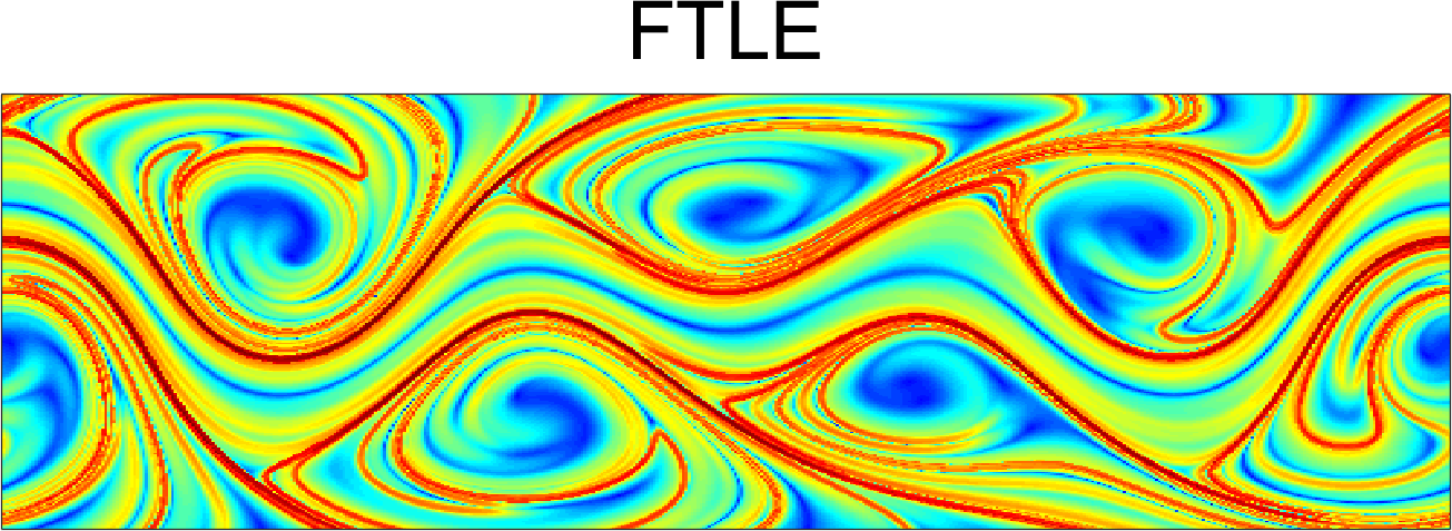
(a)

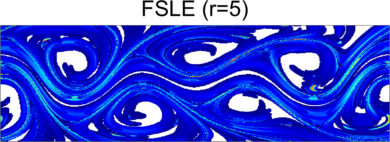
(b)

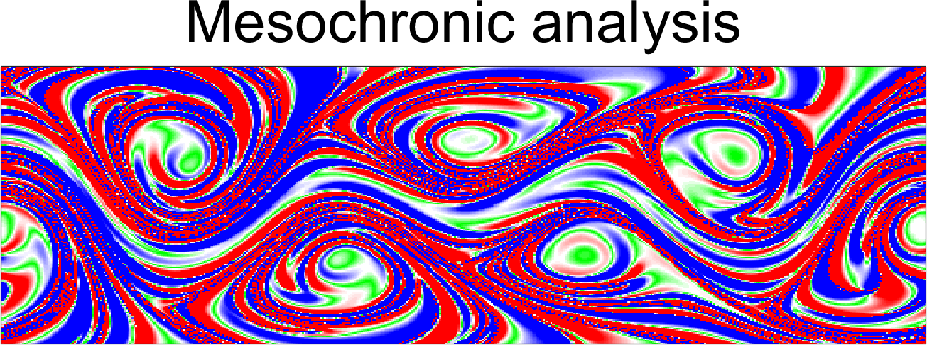
(c)

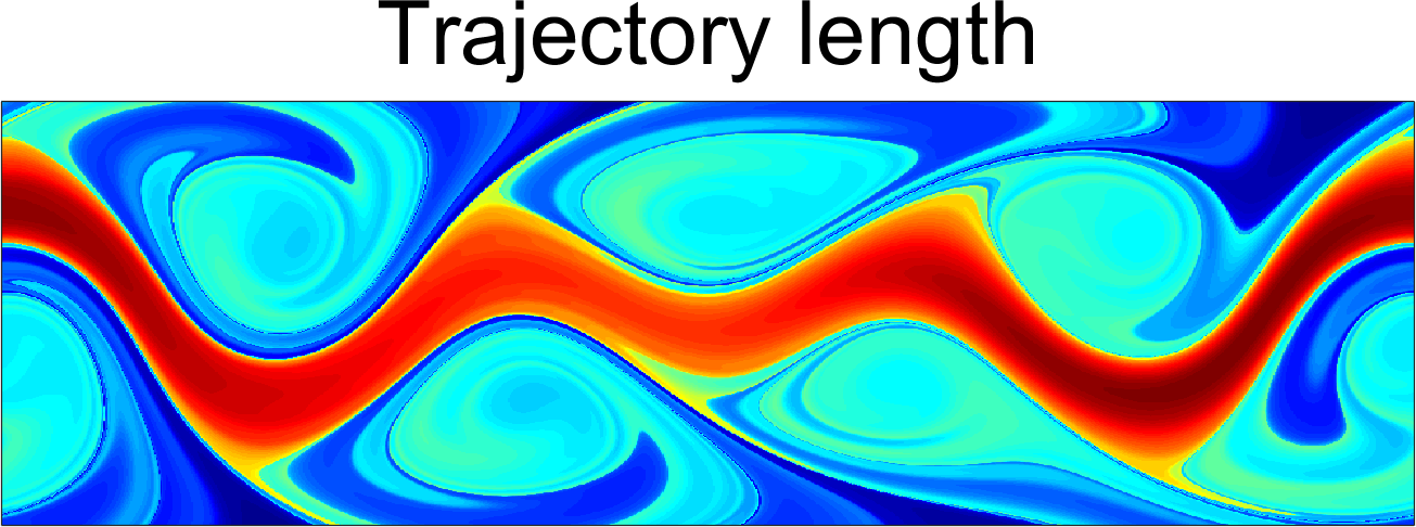
(d)

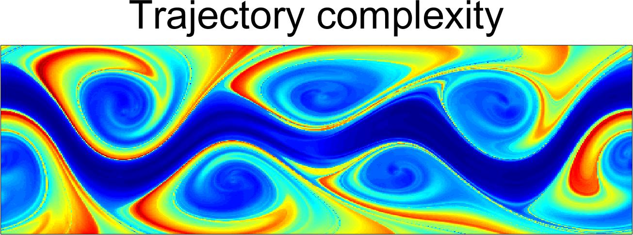
(e)

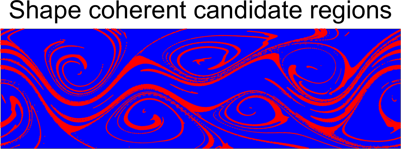
(f)

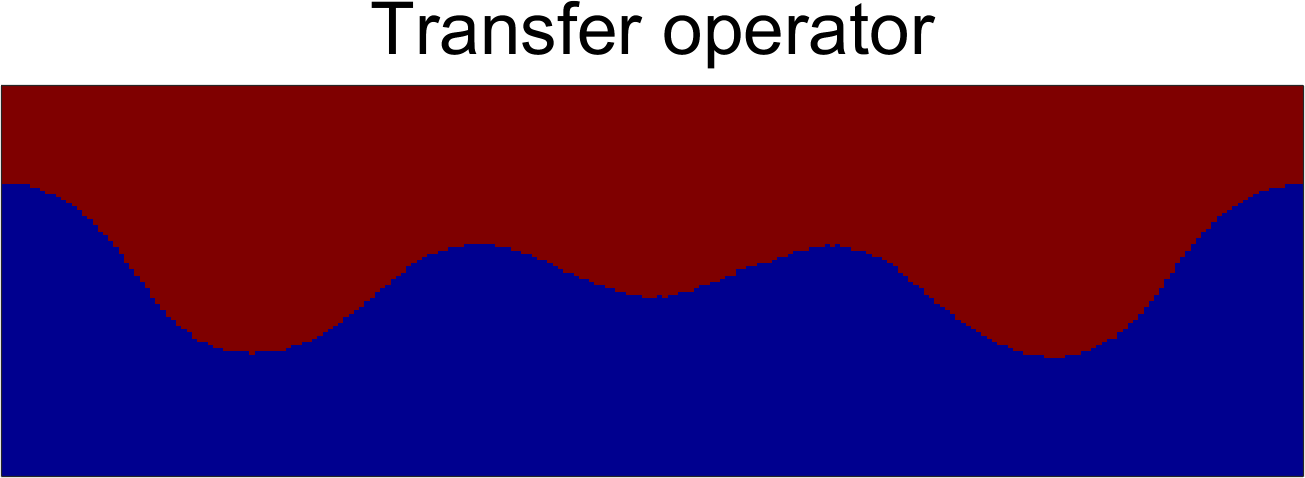
(g)

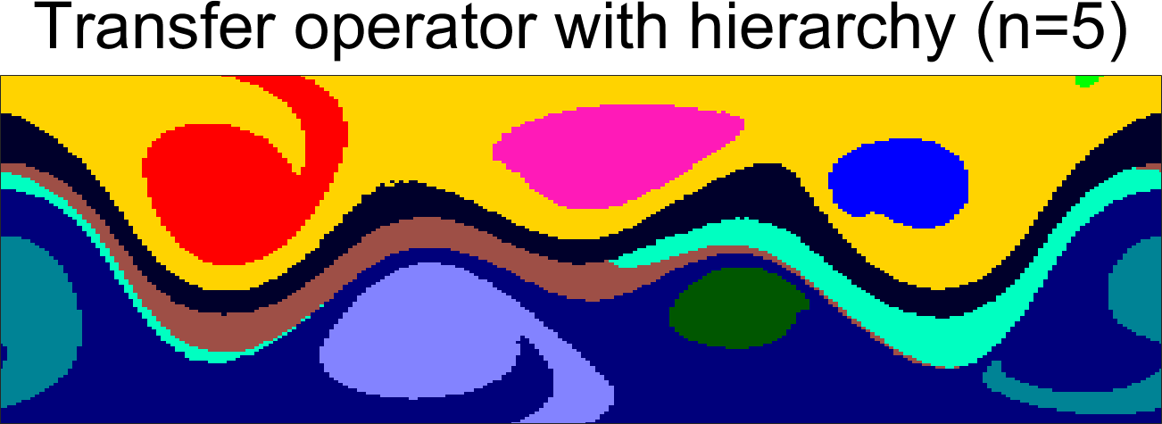
(h)

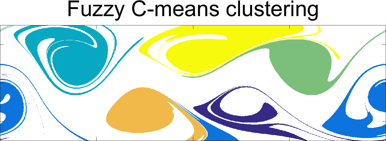
(i)

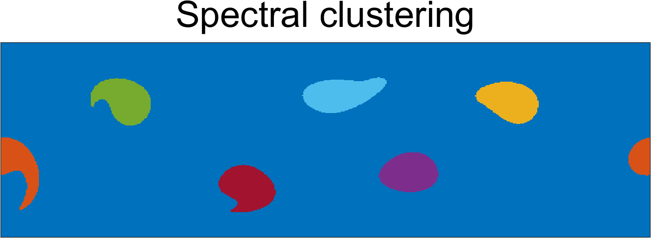
(j)

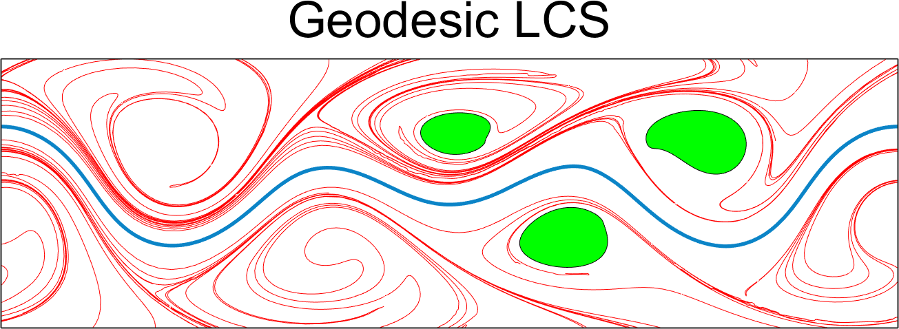
(k)

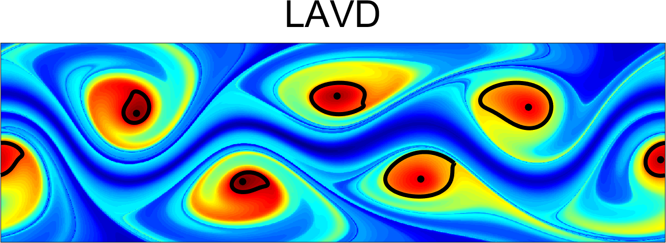
(l)

Figure 2: Comparison of Lagrangian methods on the quasiperiodic Bickley jet example (forward-time calculation only).

The majority of diagnostic scalar fields in Figure 2 indicate the presence of six vortices. Out of those offering more specific definitions for coherent structure boundaries, however, the mesochronic analysis, the shape coherence, the transfer operator and the geodesic method miss some or all of the vortices. Below, we discuss these exceptions in more detail.

Figure 2c shows the mesochronic partitioning of the domain into three different regions: mesohyperbolic without rotation (blue), mesoelliptic (green) and mesohyperbolic with rotation (red). Following the criterion proposed by Mezić Mezić (2015), we seek coherent vortex regions as nested sequences of alternating mesoelliptic and mesohyperbolic annuli with smooth boundaries (i.e., no saddle-type critical points of the mesochronic plot should be embedded in the boundary of at least three annuli of different colors). Examining fig. 5, we observe saddle-type critical points for the mesochronic field in all the vortex regions, resulting in a lack of smooth annular region boundaries. Hence, when precisely implemented, the mesochronic analysis put forward in Refs. Mezić et al., 2010; Mezić, 2015 does not indicate any coherent vortex in this example, even though the topology of mesochronic contours gives a good general indication of the vortical regions identified by objective methods. The mesochronic plot also fails to identify the hyperbolic and parabolic LCSs identified by other diagnostics, such as the FTLE field.

Figure 2f shows candidate regions (red) where shape coherent sets may exist at the initial time $t_{0}=0$. In these regions, the splitting angle between the dominant eigenvectors of the forward-time and the backward-time Cauchy–Green strain tensor is smaller than $5.7^{\circ}$. As mentioned earlier, these candidate regions are supposed to encompass vortex boundaries that have significant shape coherence over the time interval $[t_{0},t_{1}]$ of interest. In Figure 2f, however, all candidate regions are of spiral shapes, and hence cannot contain closed curves encircling the candidate regions. Consequently, the shape coherence method captures none of the coherent vortices for the Bickley jet, given that even the weakened version of the underlying criterion provides domains that cannot contain closed boundaries for these vortices.

Figure 2g shows the two coherent sets identified by the transfer operator method in this example. These two sets are precisely the upper and lower parts of the flow domain separated by the core of the jet. The jet core is identified very sharply, but the method misses the coherent vortices identified by most other methods. Higher singular vectors of the transfer operator do indicate the presence of all these vortices, even if the actual boundaries of these vortices will depend on what thresholding one uses to extract structures from the eigenfunctions. It is a priori unclear, however, how many singular vectors one needs to consider to obtain an indication of all vortices in the problem (but see below for more detail on how to make the exploration of singular vectors systematic).

Figure 2h provides a successive partitioning of the coherent sets obtained from the hierarchical transfer operator method into further coherent sets. At the fifth level of hierarchy $(n=5)$, the method captures the three most coherent vortices in the problem. These vortices will be further partitioned under subsequent steps in the hierarchical construction, unless one has a sense of the ground truth and hence knows when to stop. The increased hierarchy also dilutes the sharpness of the jet core identified by the transfer operator method. A steadily growing number of patches appear that are hard to justify physically in a perfectly homogeneous shear jet.

Figure 2i shows the results from fuzzy clustering ($K=6$, $m=1.25$). The method gives a good general sense for all coherent vortices, but indicates no well-defined coherent vortex core with a closed boundary. Instead, convoluted boundaries are detected for all vortical regions, suggesting a lack of regular, convex domains that stay tightly packed under advection. The sharp jet core detected by the transfer operator method is also absent in these results. The detected structures remain convoluted under advection in Figure 3c (Multimedia view), except for their subsets contained in coherent vortices signaled by other methods.

Figure 2j shows that the spectral clustering method consistently detects all vortices involved, improving on the estimates on their sizes given by other method. All these Lagrangian vortices do remain coherent, as confirmed by their advection in Figure 3d (Multimedia view). At the same time, the method gives no indication of the coherent meandering jet in the dominant eigenvectors $u_{1},\ldots,u_{6}$ of the graph Laplacian $L$. The seventh eigenvector $u_{7}$ does reveal the meandering jet in the flow (see Figure 5), but there is no a priori indication from the spectrum that it should. The reason is that the jet particles separate from each other due to shear, which creates notably weaker within-class-similarity for the jet than for the vortices.

Figure 2k shows the result for the geodesic LCS analysis, where elliptic LCSs (material vortices), a parabolic LCS (material jet core) and repelling hyperbolic LCSs (stable manifolds) are shown in green, blue and red, respectively. In this example, the geodesic method identifies only three out of six vortical regions as coherent. Indeed, as seen in Figure 3e (Multimedia view), only three material vortex cores with no filamentation can be found under advection to the final time $t_{1}=11$ day. (As seen in Figure 2, these three vortices also happen to be the ones most clearly identified by the hierarchical transfer operator method.) That said, Figure 3d (Multimedia view) and Figure 3f (Multimedia view) show that the actual number of arguably coherent material vortices is six, which indicates that the variational principle behind the geodesic method is too restrictive for some of the vortices of the Bickley jet flow.

Figure 2l shows that the LAVD method captures all vortices accurately and the detected structures only show tangential filamentation under advection (cf. Figure 3f (Multimedia view)), as they should by construction. At the same time, the LAVD method is unable to detect the intended main feature of this model flow, the meandering jet in the middle. More generally, the LAVD method is not designed to detect hyperbolic or parabolic LCSs.

(a)

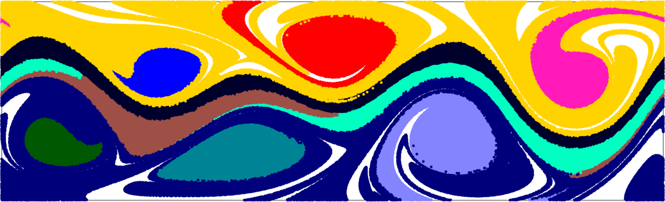
(b)

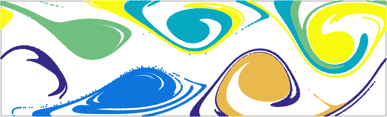
(c)

(d)

(e)

(f)

Figure 3: Advected images of Lagrangian coherent structures at the final time $t_{1}=11$ day for six different methods: (a) Probabilistic transfer operator (Multimedia view) (b) Hierarchical transfer operator (Multimedia view) (c) Fuzzy clustering (Multimedia view) (d) Spectral clustering (Multimedia view) (e) Geodesic (Multimedia view) and (f) LAVD (Multimedia view). See also Figure 6 (right) and Figure 8b for the transfer operator. Plots (a) and (b) have lower resolution because the total number of trajectories used in all computations were selected equal for a fair comparison.

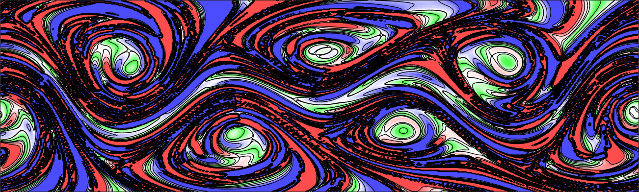
Figure 4: Mesochronic plot and its contours at the initial time $t_{0}=0$ for the quasiperiodic Bickley jet.

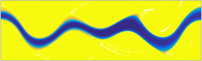
Figure 5: The seventh generalized eigenvector of the graph Laplacian $L$ obtained from the spectral clustering analysis for the quasiperiodic Bickley jet.

As for jet identification, we observe that most methods offer some indication of the central jet, except for the shape coherence, fuzzy clustering, spectral clustering and LAVD methods. The majority of methods, however, do not offer a systematic approach to extracting the jet core or jet boundaries. The only exceptions are the FTLE, geodesic and the transfer operator methods that give a sharp boundary for the jet core (see Figures 2k, 2g and 2h).

On this example, we also illustrate how a consideration of the higher singular vectors of the transfer operator yields additional insight into the structure of the two main coherent sets revealed by its second singular vector in Figure 2g. The initial domain $X=[0,20]\times[-2.5,2.5]$ (with left and right edges identified) is gridded into 125,000 identical squares (250 grid boxes in the $x$-direction and $125$ grid boxes in the $y$-direction). We use 16 uniformly distributed sample points per grid box and compute Lagrangian trajectories, recording the terminal points after time $t_{1}=24$ days. The image domain $Y=T(X)$ is gridded into squares of the same size, and is covered by 132,131 grid boxes. The grid-to-grid transition matrix $P$ (see Ref. Froyland, Santitissadeekorn, and Monahan, 2010 for details) is therefore a row-stochastic $132,131\times 125,000$ rectangular matrix. The leading singular vectors $u_{k}$ (resp. $v_{k}$), $k=2,\ldots,6$ of the transfer operator are shown in the left (resp. right) columns of Figure 6. The top row of Figure 6 shows a clear separation of the upper and lower parts of the flow domain.

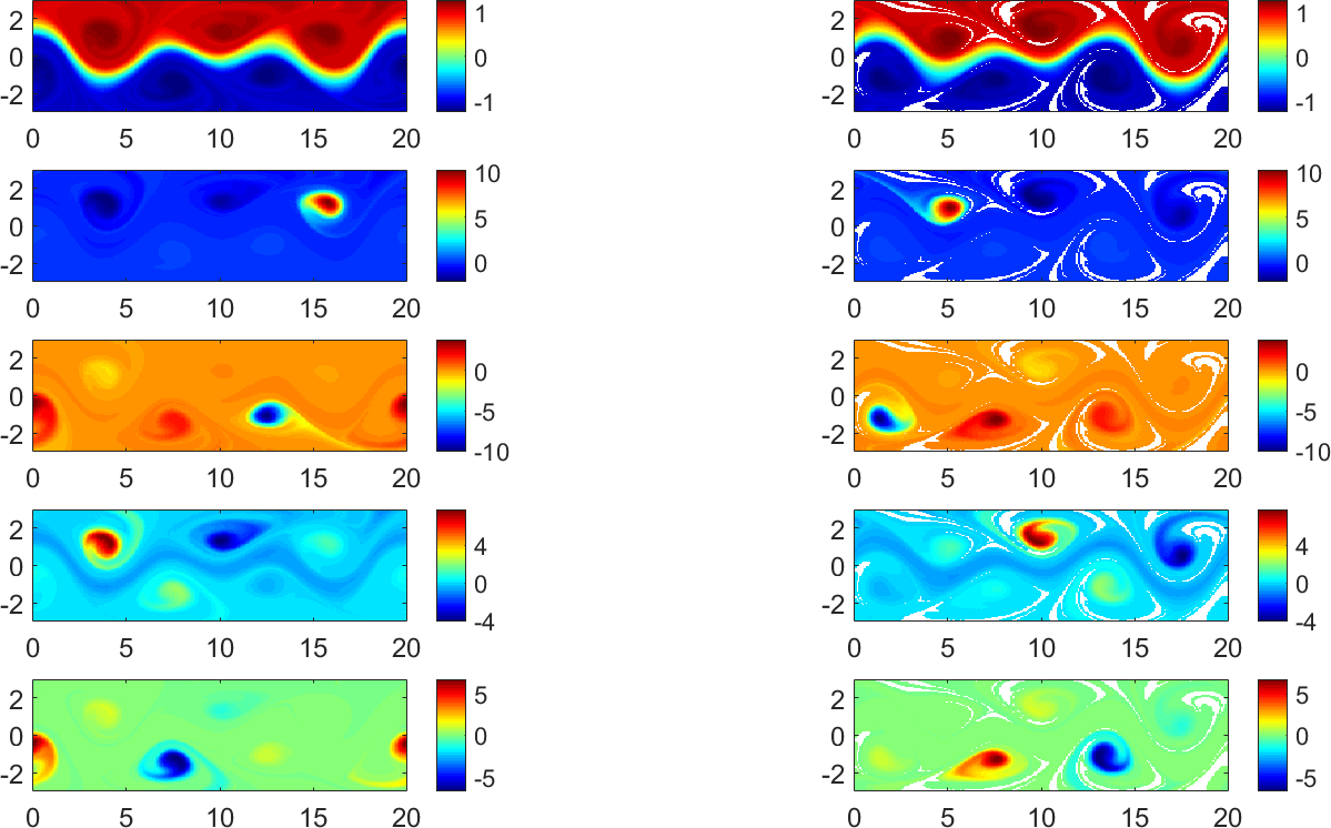
Figure 6: The first five nontrivial singular vectors of the transfer operator for the Bickley jet example. Left column: Vectors $u_{2},u_{3},u_{4},u_{5},u_{6}$ (top to bottom). Right column: Vectors $v_{2},v_{3},v_{4},v_{5},v_{6}$ (top to bottom). Various finite-time coherent sets are highlighted at the initial time (left column) and final time (right column).

We threshold the vectors $u_{2},v_{2}$ according to the algorithm proposed in Ref. Froyland, Santitissadeekorn, and Monahan, 2010 by letting $c\in\{1,\ldots,12,500\}$ represent a sorted box index. We then plot the coherence ratio $\rho(A_{c},\tilde{A}_{c})$ vs. $c$ in Figure 7 (left), where $A_{c}$, $\tilde{A}_{c}$ are super/sub-level sets of $u_{2}$, $v_{2}$ (see Algorithm 1 in Ref. Froyland, Santitissadeekorn, and Monahan, 2010 for details). In Figure 7, the blue curve indicates grid sets sorted in descending value of $u_{2}$ from the maximum of $u_{2}$, while the red curve indicates grid sets sorted in ascending value of $u_{2}$ from the minimum of $u_{2}$; the two curves meet where the mass of the partition sets are both equal to 1/2. The maximum value of $\rho(A_{c},\tilde{A}_{c})$ is indicated by the vertical arrow and the black asterisk. The resulting spatial partition is the pale yellow/pale orange separation shown in Figure 8.

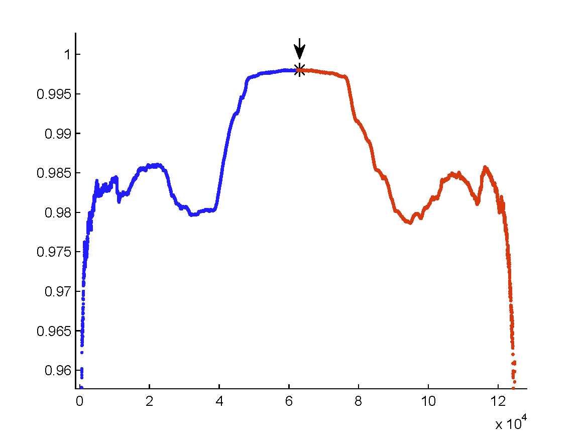
(a)

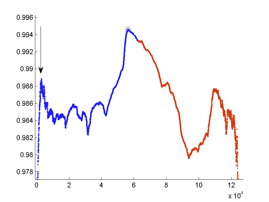
(b)

Figure 7: (a) Plot of $\rho(A_{c},\tilde{A}_{c})$ vs. $c$ based on $u_{2},v_{2}$. The global maximum of $\rho(A_{c},\tilde{A}_{c})$ is indicated with a vertical arrow and black asterisk. This corresponds to the upper/lower separation shown in pale yellow/pale orange in Figure 8. (b) Plot of $\rho(A_{c},\tilde{A}_{c})$ vs. $c$ based on $u_{3},v_{3}$. The first local maximum of $\rho(A_{c},\tilde{A}_{c})$, starting from the largest value of $u_{3}$ and descending, is indicated with a vertical arrow. This corresponds to the red set in the lower right of the upper panel of Figure 8, and its image in the lower left of the lower panel of Figure 8.

The vectors $u_{k},v_{k},k=3,\ldots,5$ in Figure 6 (second and lower rows) highlight other smaller features. In order to extract these smaller features, there are two main approaches. First, one could restrict the domain to a smaller domain, a little larger than twice the size of the highlighted feature (see, e.g., the experiments in the atmosphere Froyland, Santitissadeekorn, and Monahan (2010) and the ocean Froyland et al. (2012, 2015)). One then recomputes $u_{2}$ and $v_{2}$ and because other coherent features have been eliminated from the domain, these dominant nontrivial vectors capture the required feature. Note that this procedure is different to Ref. MA and BOLLT, 2013.

Second, one could retain the original domain and use the vectors $u_{k},v_{k},k=2,\ldots,5$ directly. Various techniques have been devised to extract information from multiple vectors (see, e.g., the references in 3.1 of Ref. Froyland and Padberg, 2009). One could, for instance, fuzzy cluster the embedded vectors $u_{k}$,Froyland (2005). Here we take a vector by vector approach. In the present example, there are clear features highlighted through the extreme negative or positive values of $u_{k},v_{k},k=3,\ldots,5$. In general, given a particular sufficiently coherent spatial feature, one should always be able to find a vector which highlights that feature through an extreme negative or positive value (for example, see Fig. 4 of Ref. Froyland, Stuart, and van Sebille, 2014 for computations on the global ocean). A simple approach is to look for the first local maxima of $\rho(A_{c},\tilde{A}_{c})$ in the thresholding figures computed from $u_{k},v_{k},k=3,\ldots,5$, starting at either the negative or positive end of the vector that corresponds to the spatial feature one wishes to extract.

For example, the second row of Figure 6 highlights a small red feature, which corresponds to a extreme positive values of $u_{3},v_{3}$. Thus, we threshold starting from the maxima of $u_{3},v_{3}$ and descend, looking for the first local maximum of $\rho(A_{c},\tilde{A}_{c})$. Figure 7 (right) shows the full plot of $\rho(A_{c},\tilde{A}_{c})$ vs. $c$, with the first local maximum indicated with a vertical black arrow. The corresponding spatial feature is shown in the lightest red in Figure 8. This approach is repeated for all remaining highlighted features in Figure 6 . The extracted finite-time coherent sets are displayed in Figure 8.

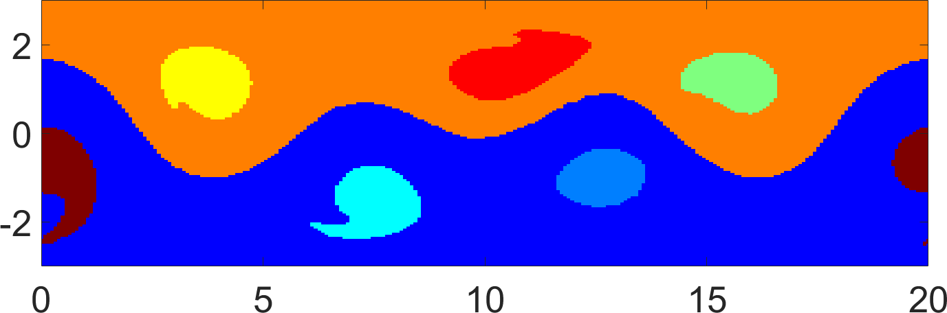
(a)

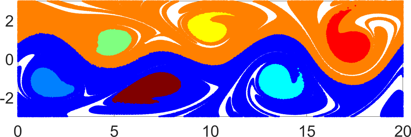
(b)

Figure 8: (a) The finite-time coherent sets extracted from the singular vectors $u_{k},v_{k},k=2,\ldots,6$ for the Bickley jet example at the initial time. (b) Advected image of the coherent sets at the final time.

V.2 Two-dimensional turbulence

As our second example, we consider a flow without any temporal recurrence. We solve the forced Navier–Stokes equation

$$\partial_{t}v+v\cdot\nabla v=-\nabla p+\nu\Delta v+f,\quad\nabla\cdot v=0,$$ (33)

for a two-dimensional velocity field $v(x,t)$ with $x=(x_{1},x_{2})\in U=[0,2\pi]\times[0,2\pi]$. We use a pseudo-spectral code with viscosity $\nu=10^{-5}$ on a $512\times 512$ grid, as described in Ref. Farazmand and Haller, 2013. A random-in-phase velocity field evolves in the absence of forcing ($f=0$) until the flow is fully developed. At that point, a random-in-phase forcing is applied. For the purposes of the following Lagrangian analysis, we identify this instance with the initial time $t=0$. The finite time interval of interest is then $t\in[0,50]$.

Figure 9 shows the result from various Lagrangian methods applied to the resulting finite-time dynamical system $\dot{x}=v(x,t)$. We use the auxiliary gird approach with the distance $\rho=10^{-3}$ to construct the FTLE, FSLE, mesochronic and shape coherence diagnostic fields. The same auxiliary distance is used to compute the Cauchy–Green strain tensor as well as the vorticity for the geodesic and LAVD methods, respectively.

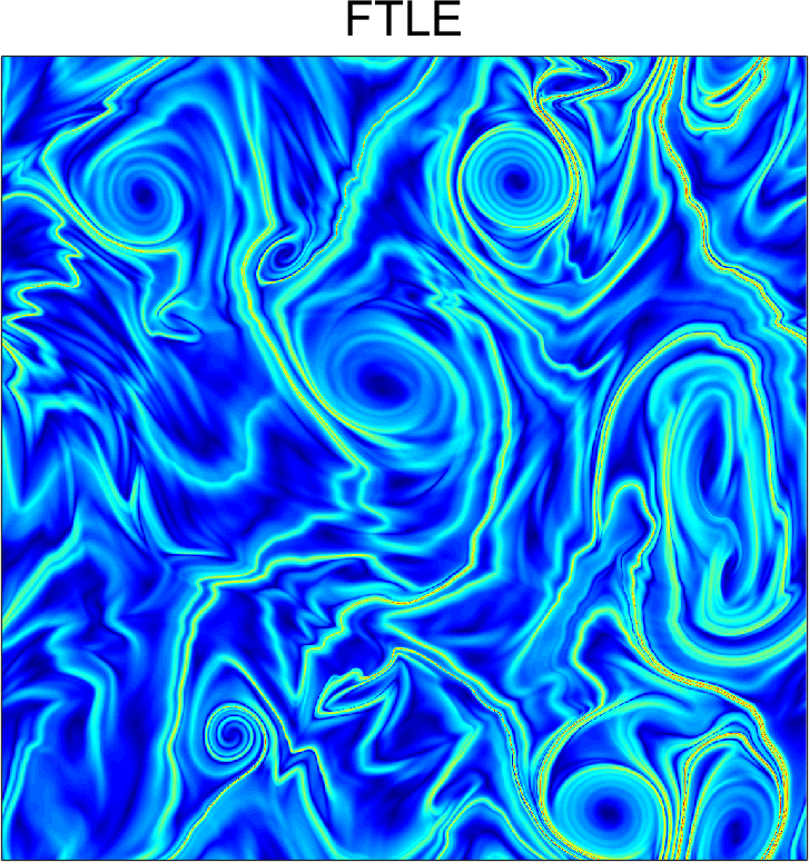
(a)

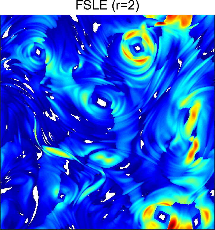
(b)

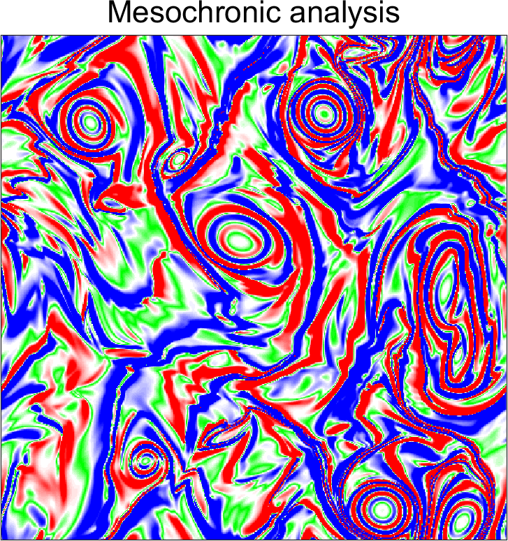
(c)

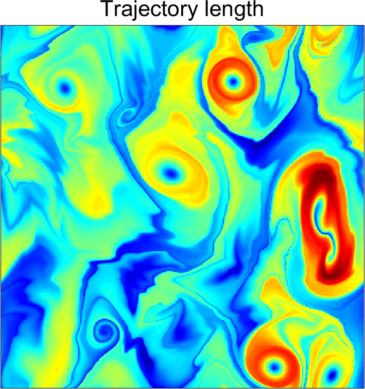
(d)

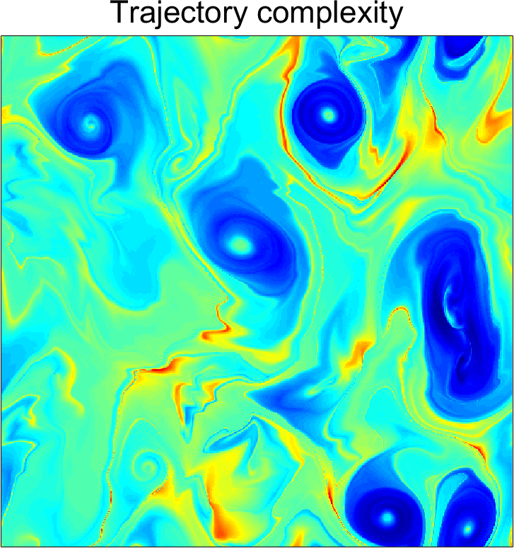
(e)

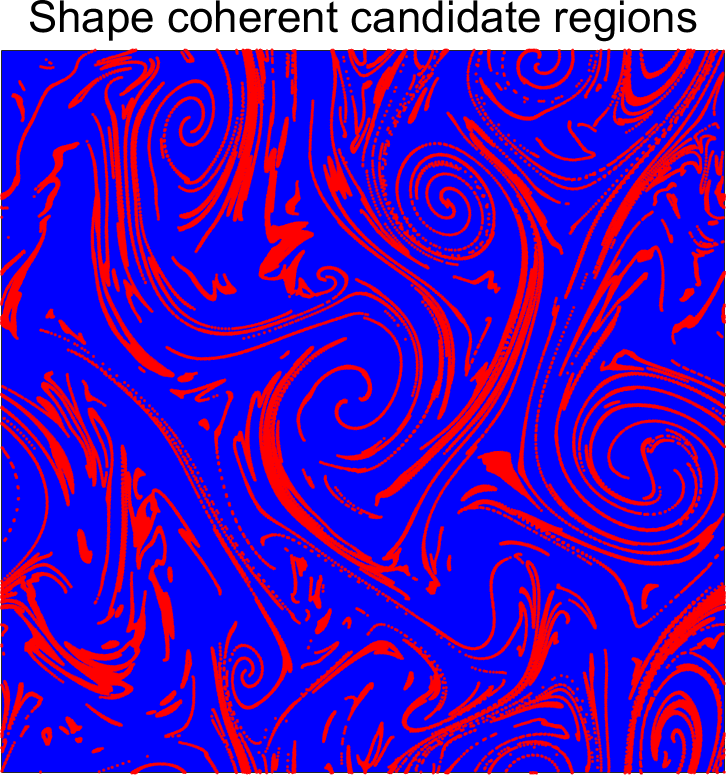
(f)

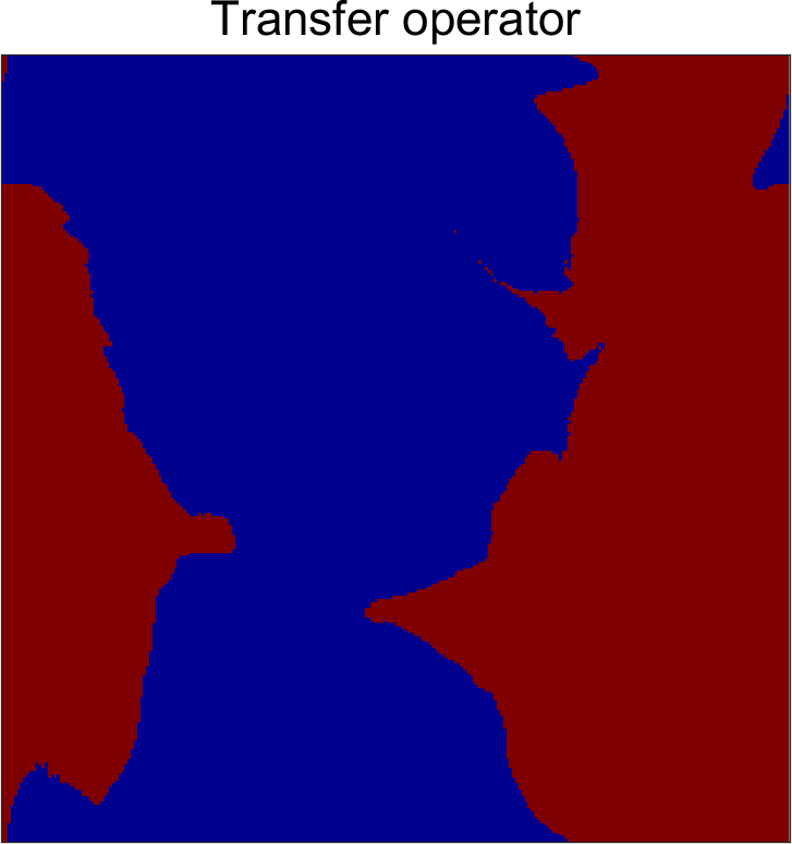
(g)

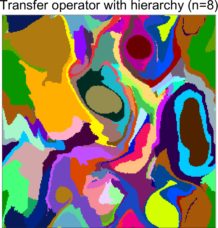
(h)

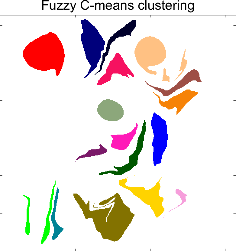
(i)

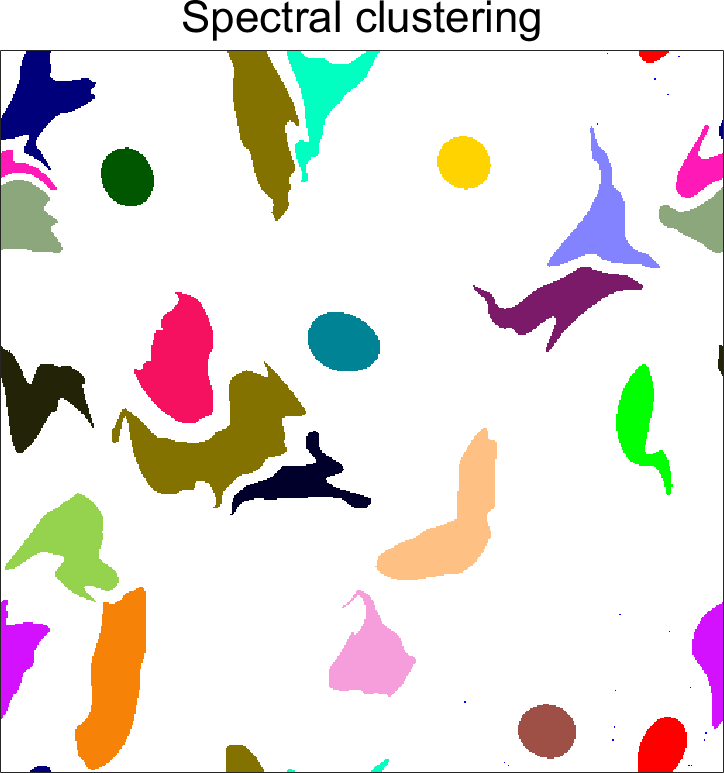
(j)

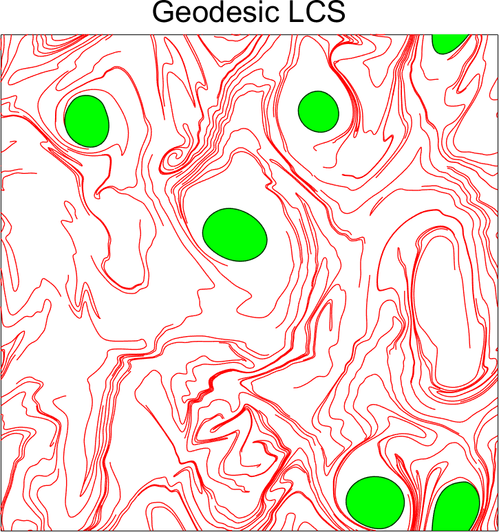
(k)

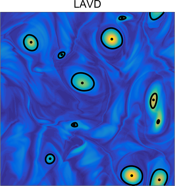
(l)

Figure 9: Comparison of Lagrangian methods on the two-dimensional turbulence simulation example.

Most plots in Figure 9 indicate several vortex-type structures, except for the shape coherence and transfer operator methods. While the boundaries of the large-scale coherent sets identified by the latter method indeed do not grow significantly under the finite-time flow, these sets are unrelated to the vortices that are generally agreed to be the coherent structures of two-dimensional turbulence. These vortices only appear in some of the higher singular vectors of the transfer operator, similarly to Figure 6 and Figure 8. Just as in the case of the Bickley jet, however, there is no clear indication from the spectrum of singular values for the number of singular vectors to be considered to recover all vortices.

The hierarchical application of the transfer operator method MA and BOLLT (2013) also signals vortex-like structures but these no longer stand out of the many additional patches it labels as coherent sets. Most of these patches appear to be examples of coincidental, rather than physical, coherence with respect to the coherence metric imposed by the method. An additional issue with the hierarchical transfer operator method MA and BOLLT (2013) is its convergence on this example. The method sets a threshold on the relative improvement of the coherence with respect to the reference probability measure $\mu$, which needs to be computed and satisfied over consecutive refinements of coherent pairs. However, at each iteration, $\mu$ depends on the initial numerical diffusion imposed by the box covering. As a consequence, identifying similar coherent sets under various box covering resolutions requires different threshold values. Figure 10 shows the hierarchical coherent sets obtained with a fixed termination threshold for three different box covering resolutions. Figure 10 indicates no overall convergence, except in some minor details.

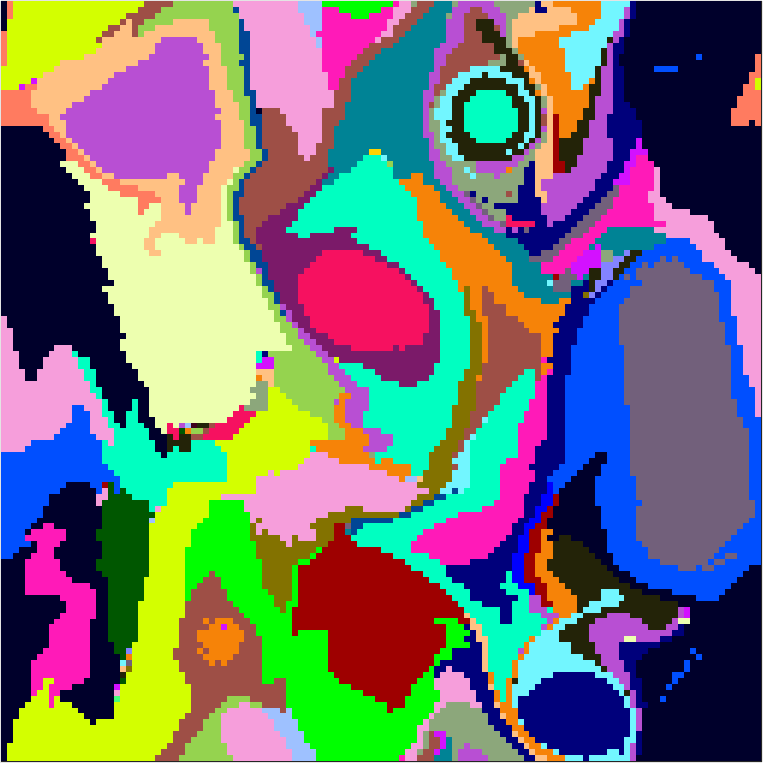
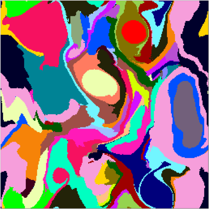
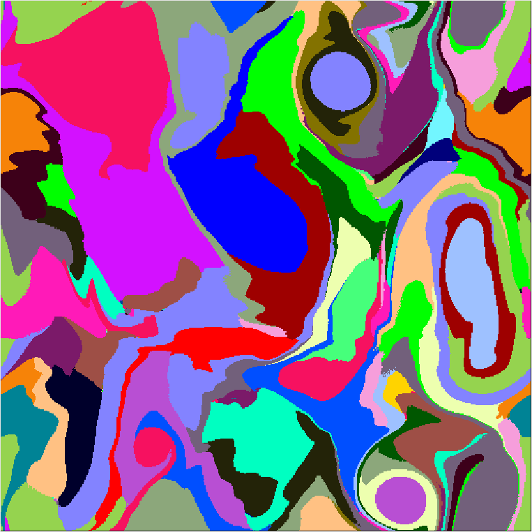
Figure 10: Hierarchical transfer operator method with $128$ (left), $256$ (middle) and $512$ (right) boxes. For all cases: Each box contains $16$ points; $8$ levels of hierarchy where used; and $\mu$-tolerance is set to $5\times 10^{-2}$.

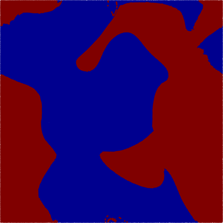
(a)

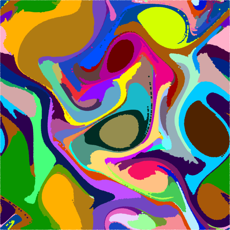
(b)

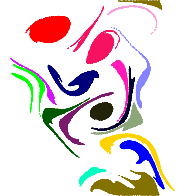
(c)

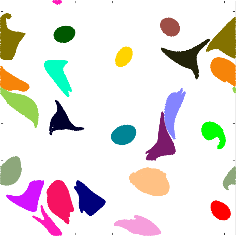
(d)

(e)

(f)

Figure 11: Advected images of Lagrangian coherent structures at the final time $t_{1}=50$ for six different methods: (a) Probabilistic transfer operator (Multimedia view) (b) Hierarchical transfer operator (Multimedia view) (c) Fuzzy clustering (Multimedia view) (d) Spectral clustering (Multimedia view) (e) Geodesic (Multimedia view) and (f) LAVD (Multimedia view). Plots (a) and (b) have lower resolution because the total number of trajectories used in all computations were selected equal for a fair comparison.

Figure 9f shows candidate regions (red) where shape coherent sets may exist at the initial time $t_{0}=0$. In these regions, the angle between stable and unstable foliations is smaller than $5.7^{\circ}$, and hence all vortex boundaries should be fully contained in these regions. Inspection of Figure 9f, however, reveals that these candidate regions are spirals, and hence no closed vortex boundaries satisfying the shape coherence requirement exist. This is unsurprising as the underlying coherence principle is only arguable for flows whose behavior is the same in forward and backward time, which is not the case for the present example.

Figure 9j shows the coherent sets detected by the spectral clustering method at the initial time. These coherent sets include the vortices captured by the Geodesic and LAVD methods, as well as some additional structures. Figure 11d (Multimedia view) illustrates that the advected image of these additional coherent sets indeed show limited dispersion at the final time $t_{1}=50$. As in the case of hierarchical transfer operator method, some of these moderately dispersive sets are of irregular, physically unexpected shape. A systematic comparison with the results of the FTLE analysis (see Figure 9a) shows that all these irregularly shaped regions are valleys of low FTLE values among FTLE ridges. Therefore, beyond coherent vortices, spectral clustering also identifies domains that are trapped between finite-time stable manifolds of saddle-type (hyperbolic) trajectories. This feature may make spectral clustering the method of choice in applications with a well-defined time scale of interest (e.g., fixed-time forecasting problems). At the same time, there is no a priori constraint in a turbulent flow that keeps stable manifolds of different hyperbolic trajectories close to each other. For this reason, several of the irregularly shaped sets identified from spectral clustering may change substantially under changes in the extraction interval.

Figure 9i shows that fuzzy clustering (with $m=1.5$ and $K=20$) also identifies both regularly and irregularly shaped coherent sets. Three of these clearly indicate coherent vortices, containing the coherent vortices indicated by other methods in these locations. Since these larger vortices predicted by fuzzy clustering only show tangential filamentation (cf. Figure 11c (Multimedia view) ), this method gives the sharpest, least conservative assessment of coherence for these vortices relative to the results returned by other methods. That said, the method also completely misses the remaining two, highly coherent larger vortices. Furthermore, the irregularly shaped domains identified by fuzzy clustering lose their coherence by the end time of the extraction interval, showing stretching and filamentation in Figure 11c (Multimedia view). The total number of extracted sets (the number $K$ of clusters) is an input parameter for the method, so the number of inaccurate coherence predictions are influenced by choices made by the user.

Figure 9k shows the geodesic Lagrangian vortex boundaries (green) as well as the repelling hyperbolic LCSs (red) at the initial time $t_{0}=0$. Coherent Lagrangian vortex boundaries (black) are defined as the outermost members of nested elliptic LCS families. In Figure 11e (Multimedia view), we confirm the sustained coherence of the geodesic vortex boundaries by advecting them to the final time $t_{1}=50$. At the same time, other methods (e.g., the LAVD method discussed below) reveal additional vortices that should also be considered coherent based on their advection properties, as they only exhibit limited tangential filamentation. The geodesic method, is therefore, too conservative to detect these smaller vortices.

Figure 9l shows the Lagrangian vortex boundaries extracted using the LAVD method at the initial time $t_{0}=0$. In this computation, we have set the minimum arc-length, $l_{min}=0.3$ and convexity deficiency bound $d_{max}=0.005$. In Figure 11f (Multimedia view), we confirm the Lagrangian rotational coherence of these vortex boundaries by advecting them to the final time $t_{1}=50$. As guaranteed by the derivation of the LAVD method, the vortex boundaries display only tangential filamentation. With this relaxed definition of coherence, the LAVD approach identifies additional smaller vortices missed by the geodesic LCS method (cf. Figure 9k). At the same time, the LAVD method only targets vortices, missing other patches of trajectories that remain closely packed over the same time interval (see, e.g., the discussion on spectral clustering above).

Beyond showing the results of various methods, we also use this example to investigate whether contours of diagnostic tools such as the trajectory length function or mesochronic field can be used for the purpose of vortex boundary detection. Specifically, we extract the contours of these two diagnostic methods for two select vortex regions at initial time $t_{0}=0$, and advect them to the final time $t_{1}=50$. In addition, we make a comparison with the geodesic vortex boundaries obtained for the same regions.

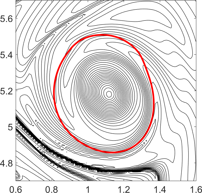
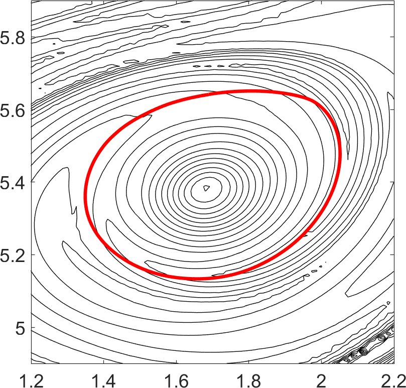
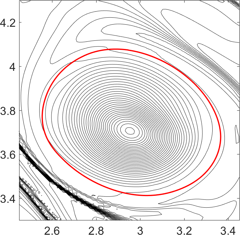
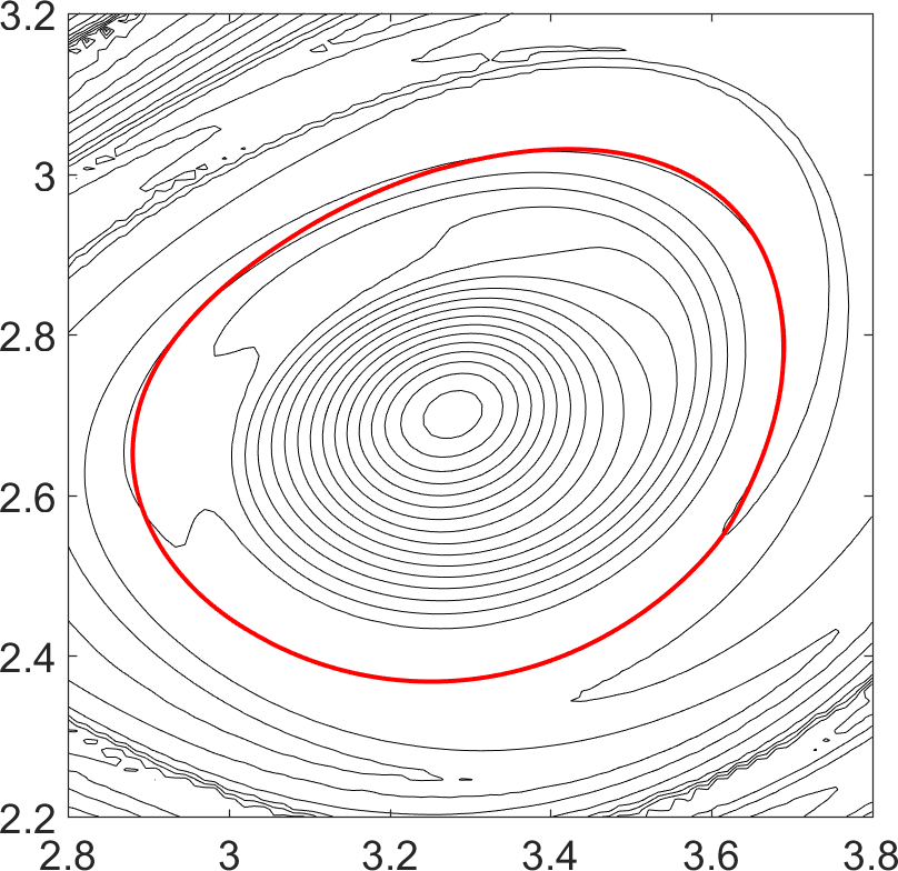
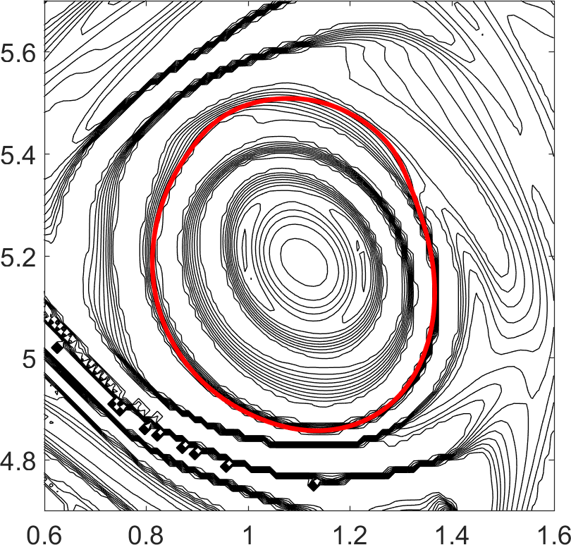
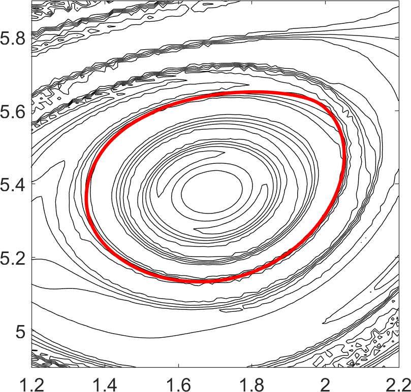
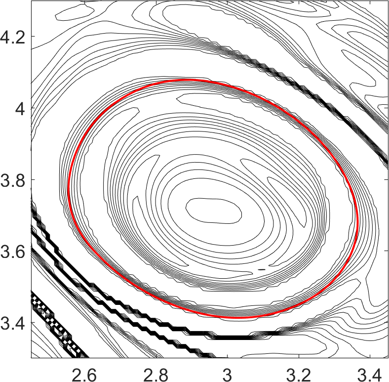
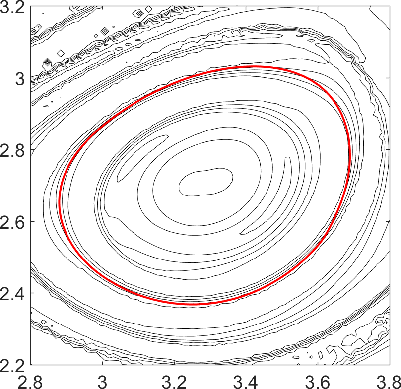
Figure 12: M-function contours (black curves) and the geodesic vortex boundary (red curves) at the initial time $t=0$ (left) and at the final time $t=50$ (right).

Figure 13: Contours of the mesochronic scalar (black curves) and the geodesic vortex boundary (red curves) at the initial time $t=0$ (left) and at the final time $t=50$ (right).

Figure 13 shows the advection of the level-curves of the trajectory length function $M_{0}^{50}$ around two select vortices. The level-curves closer to the vortex core remain coherent for both vortices. A comparison with the geodesic vortex boundary, however, shows that the contours of $M_{0}^{50}$ underestimate the size of the upper vortex substantially. A precise implementation of the mesochronic vortex criterion of Ref. Mezić, 2015 shows again a lack of vortex-type structures in the selected regions due to presence of the saddle-type critical points. In contrast, a visual inspection of the same regions in Figure 9, without implementing the specific vortex criterion of Ref. Mezić, 2015, does suggest coherent vortices in all vortical regions identified by the geodesic and the LAVD method. The actual boundaries of the vortices, however, cannot be inferred based on such an inspection.

V.3 Wind field from Jupiter’s atmosphere

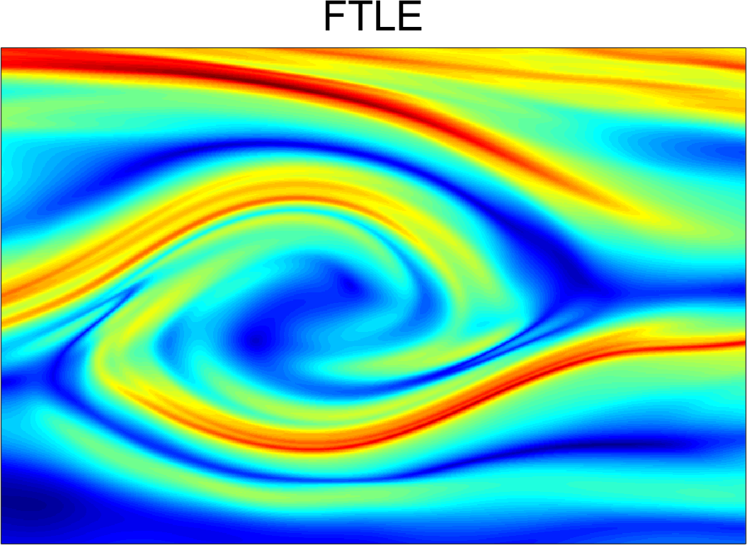
(a)

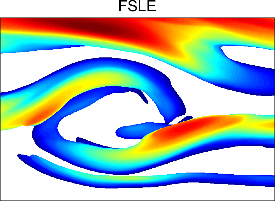
(b)

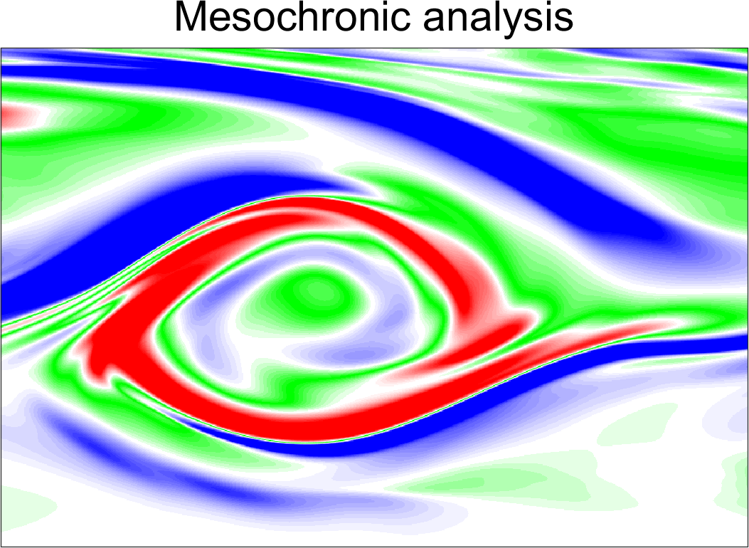
(c)

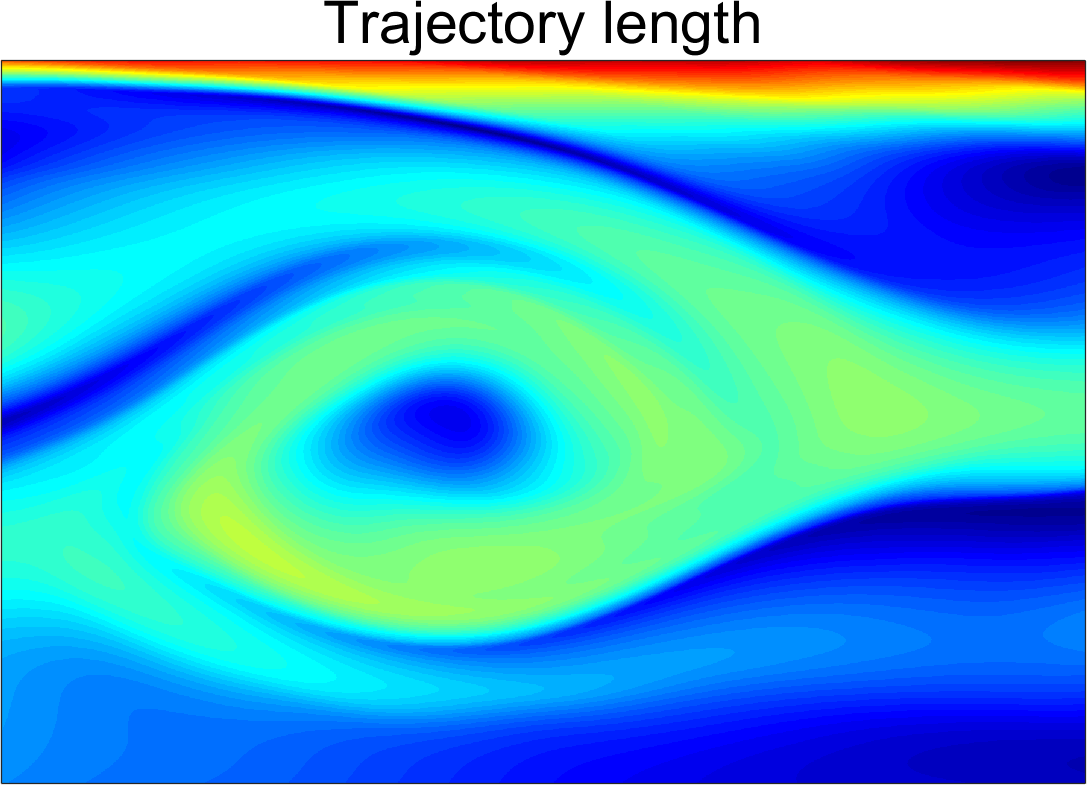
(d)

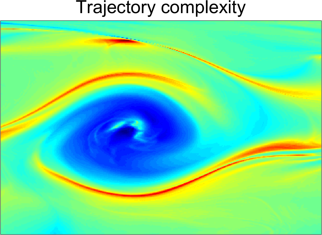
(e)

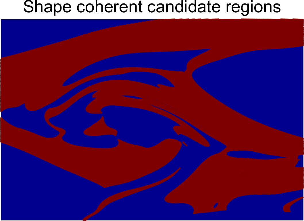
(f)

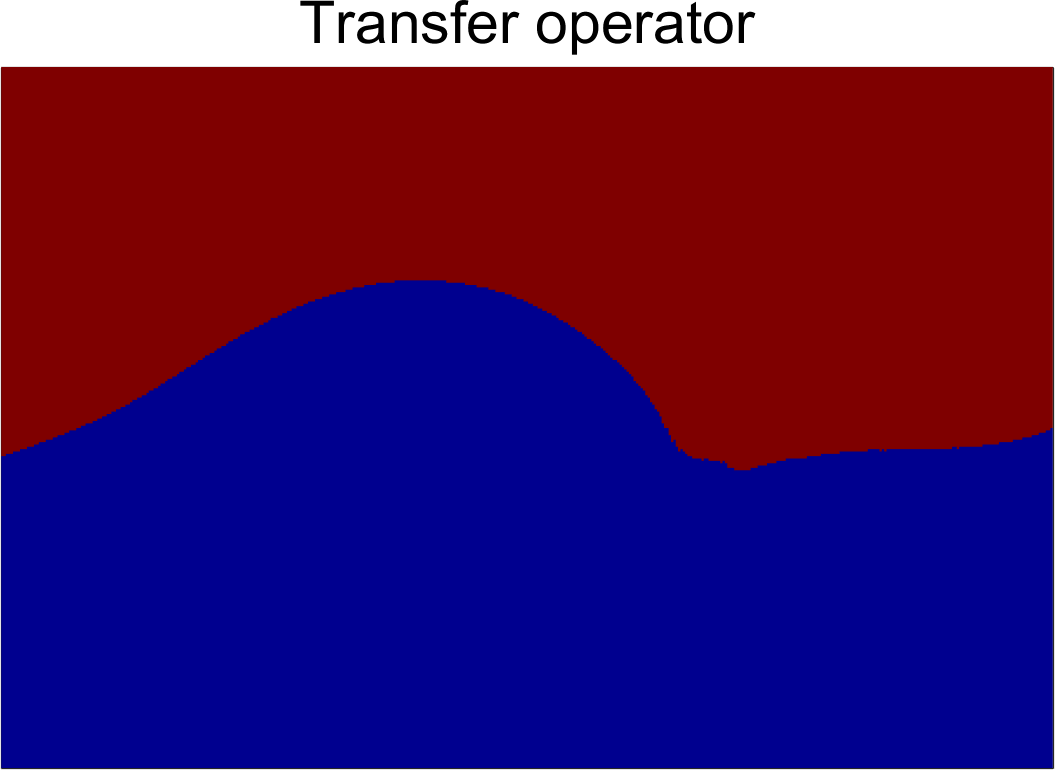
(g)

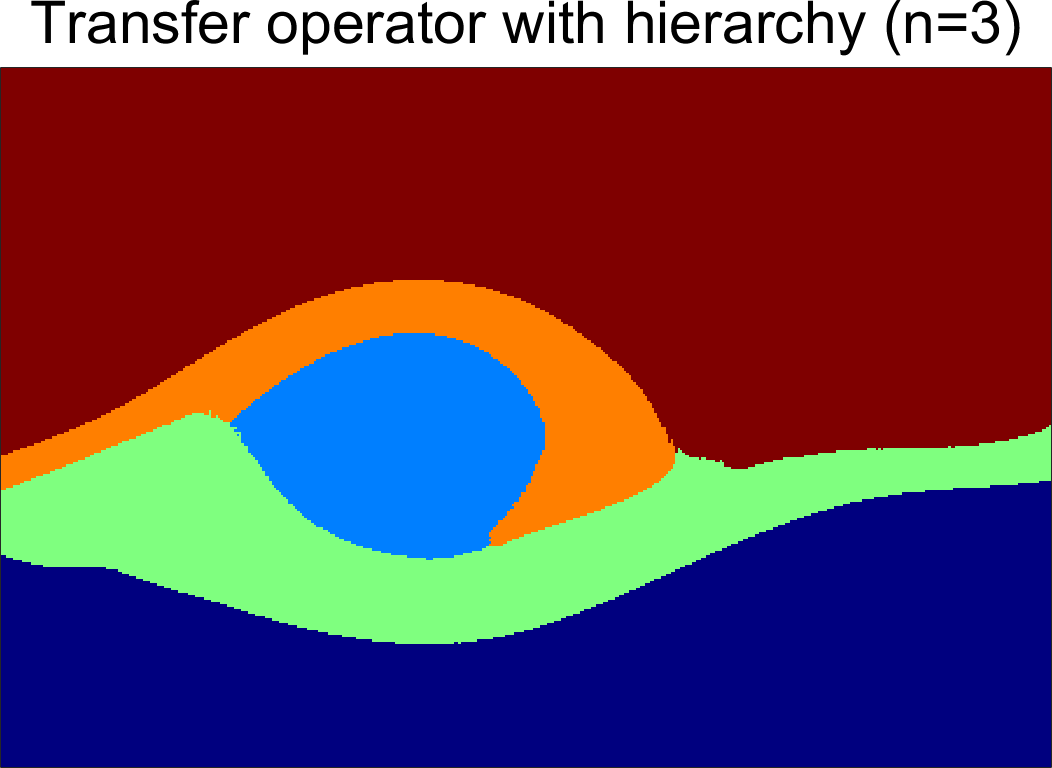
(h)

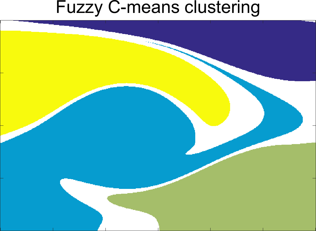
(i)

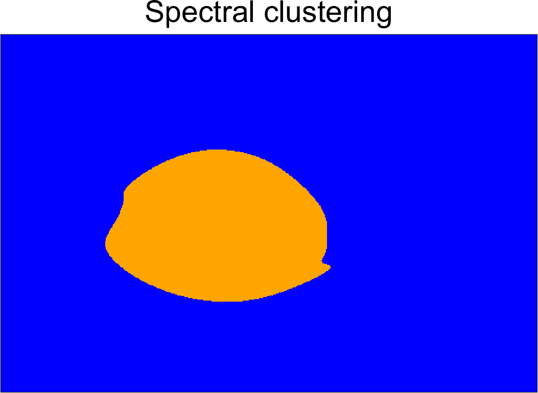
(j)

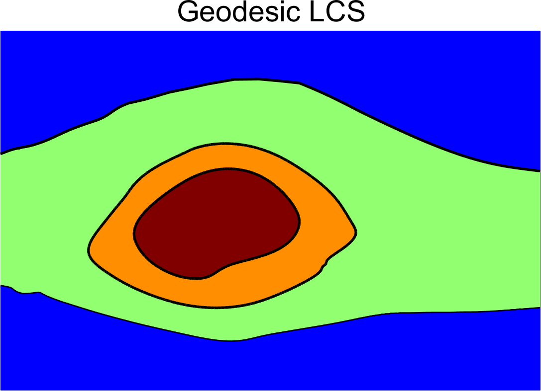
(k)

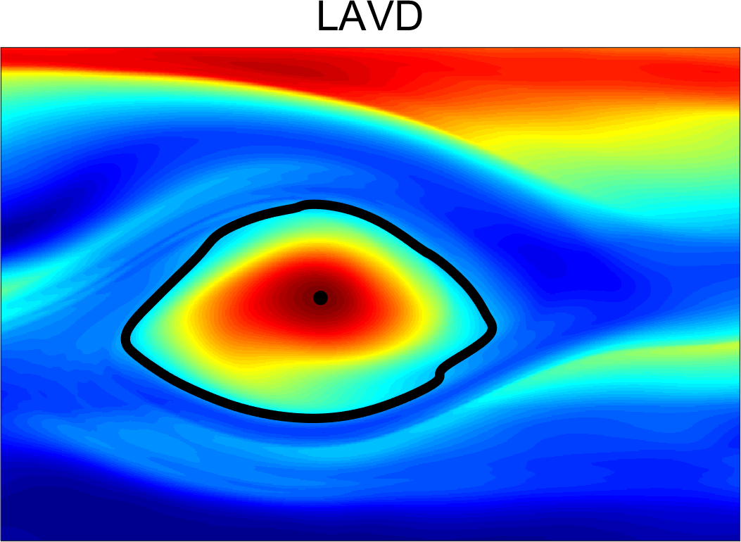
(l)

Figure 14: The output of all methods at initial time $t_{0}$ for Jupiter’s wind-velocity field of Ref. Hadjighasem and Haller, 2016b.

In our third example, we compare the twelve Lagrangian structure detection methods on an unsteady velocity field extracted from video footage of Jupiter’s atmosphere. The video footage was acquired by the Cassini spacecraft, covering $24$ Jovian days, ranging from October 31 to November 9 in year 2000. To reconstruct the velocity field, we used the Advection Corrected Correlation Image Velocimetry (ACCIV) method Asay-Davis et al. (2009) to obtain high-density, time-resolved velocity vectors (cf. Ref. Hadjighasem and Haller, 2016b for details). This is a characteristically finite-time problem: no further video footage and hence no further time-resolved velocity data are available outside the time interval analyzed here. Furthermore, the data was acquired in a frame orbiting around Jupiter, and hence the frame-invariance of the results is a crucial requirements.

In this example, we use a total number of $1800\times 1200$ particles for all the methods. The spatial domain $U$ in question ranges from $-61.6^{\circ}$ W to $-31.6^{\circ}$ W in longitude and from $-8.9^{\circ}$ S to $-28.9^{\circ}$ S in latitude. We perform the computation of gradient-based approaches, such as FTLE, FSLE, mesochronic, shape coherence and geodesic LCS analysis, using an auxiliary grid to ensure high-precision and numerical stability in the finite differencing. Specifically, an embedded grid of resolution $900\times 600$ is used to construct the corresponding scalar fields. In contrast, we use a uniform grid of $1800\times 1200$ for the gradient-free methods. As for the transfer-operator-based approaches, we use a grid of $450\times 300$ boxes, with $16$ uniformly uniformly sampled points per grid box. Here, we use a variable-order Adams–Bashforth–Moulton solver (ODE113 in MATLAB), with relative and absolute tolerances of $10^{-6}$, for trajectory advection. We obtain the velocity field at any given point by interpolating the velocity data set using bilinear interpolation.

As seen in Figure 14, several methods that offer specific structure boundary definitions signal a localized, vortex-type coherent structure corresponding to the Great Red Spot (GRS) of Jupiter. Exceptions to this rule are the transfer operator, shape coherence, fuzzy clustering and the mesochronic method. The 5th singular vector (not shown here) of the transfer operator does give an indication of the GRS, similarly to Figures 2 and 9. As in our pervious examples, however, an inspection of the singular value spectrum of the transfer operator does not a priori suggest a distinguished role for the 5th singular vector.

As in our previous example, the hierarchical transfer operator method also signals a localized vortex-like structure (see Figure 14h). The precise implementation of the mesochronic vortex criterion of Ref. Mezić, 2015 provides again no coherent vortex boundary due to the lack of a nested sequence of smooth closed contours. An intuitive visual inspection of the mesochronic plots still suggests a vortical structure to the extent that other heuristic diagnostics do (the FTLE, FSLE, M-function and trajectory complexity methods).

Spectral clustering, geodesic LCS detection and the LAVD method give very close results for the boundary of the GRS in this example. This suggests that the core of the Great Red Spot is a fairly well defined material vortex with negligible material filamentation.

As for jet identification, most diagnostic methods in Figure 14 give some indication of two jets passing north and south of the GRS. However, since these methods give no clear recipe for jet identification, we could not go beyond a general visual assessment of the results. In contrast, the transfer operator, the hierarchical transfer operator and the geodesic LCS methods suggest clear jet cores or jet boundaries. The ones signalled by the geodesic LCS method also coincide with zonal jet cores observed visually in Jupiter’s atmosphere Hadjighasem and Haller (2016b).

As in the earlier two examples, fuzzy clustering (with $m=1.25$ and $K=4$) gives convoluted structure boundary candidates, some of which stretch out significantly under advection in Figure 15c. The observed stretch in these boundaries is unsurprising, given that they are transverse to known transport barriers (shear jets) in the atmosphere of Jupiter. Together with our earlier Bickley jet example, the present example indicates a difficulty for fuzzy clustering to identify vortical and jet-type structures when both are present.

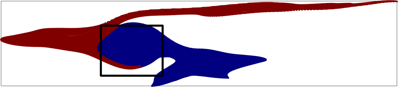
(a)

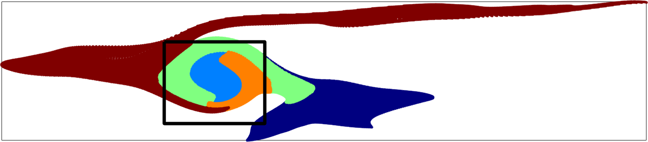
(b)

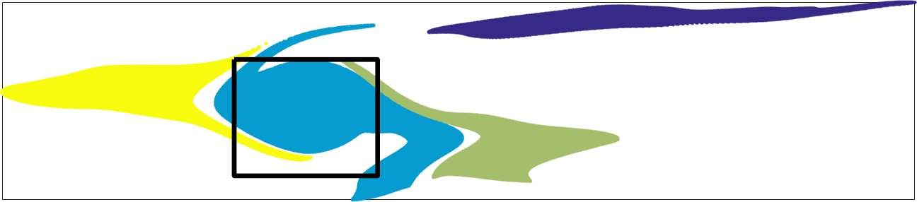
(c)

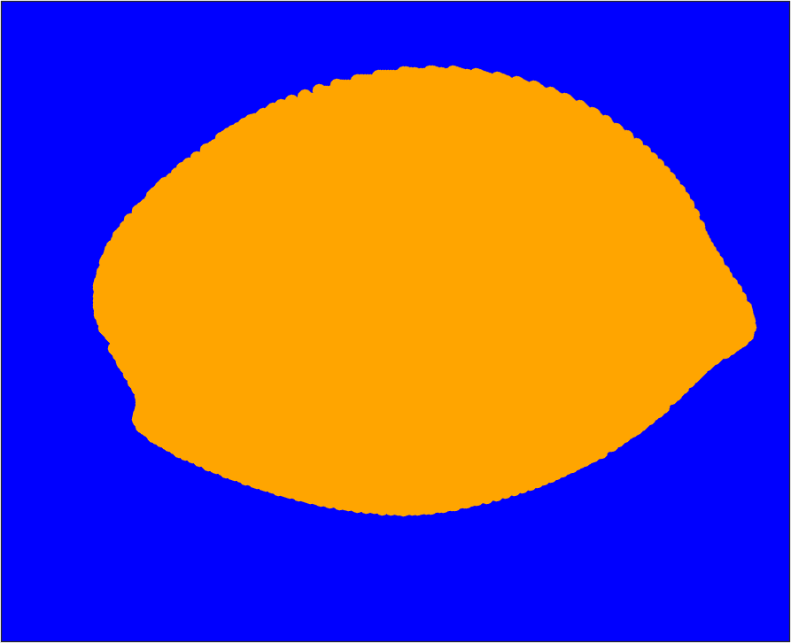
(d)

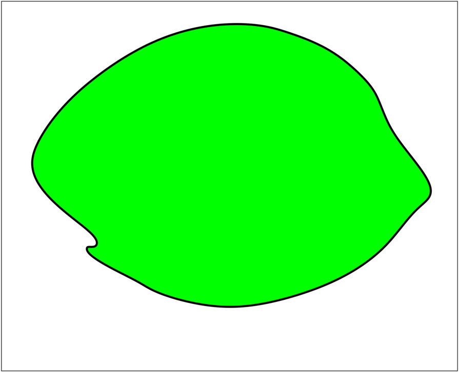
(e)

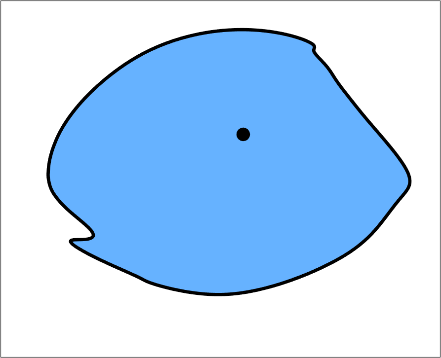
(f)

Figure 15: Advected images of Lagrangian coherent structures at the final time $t_{1}=24$ for six different methods: (a) Probabilistic transfer operator (Multimedia view) (b) Hierarchical transfer operator (Multimedia view) (c) Fuzzy clustering (Multimedia view) (d) Spectral clustering (Multimedia view) (e) Geodesic (Multimedia view) and (f) LAVD (Multimedia view). Plots (a), (b) and (c) are constructed using the advected image of the original rectangular domain of Figures 14g, 14h and 14i, respectively. In these plots, the box framing the plots (d), (e), and (f) is shown in black for reference.

In Figures 15a, 15b and 15c (Multimedia view), we advect to the final time $t_{1}=24$ the initial rectangular domain and the partitioning of this domain into sets identified as coherent by the probabilistic transfer operator, hierarchical transfer operator, and fuzzy clustering methods. A zoom-in of the advected image of the single subset identified as coherent by the spectral clustering, geodesic LCS, and LAVD methods is shown in Figures 15d, 15e and 15f (Multimedia view). As noted above, coherent regions predicted by the transfer operator and the transfer operator with hierarchy have common boundaries that remain short by construction. At the same time, the advected domain boundaries (which are beyond the control of these methods) stretch substantially over the time interval of advection. In contrast, all boundary components of the regions identified by the fuzzy clustering as coherent either are long at the initial time or stretch under advection, defying expectations for coherence. Finally, all structure boundaries predicted by the spectral clustering, geodesic LCS and LAVD methods stay coherent.

VI Assessment

Based on our three benchmark examples and available evidence in the literature, we now summarize the inferred strengths and weaknesses of the twelve Lagrangian methods compared here:

VI.0.1 FTLE method

Strengths

simple and objective algorithm; FTLE ridges capture hyperbolic LCSs under additional mathematical conditions (cf. Ref. Haller, 2011); FTLE trenches tend to approximate jet cores (but see Ref. Farazmand, Blazevski, and Haller, 2014 for exceptions).

Weaknesses

no reliable detection of elliptic LCSs; ridges connect locations of high stretching with those of high shear, and hence also produce false positives for hyperbolic LCS.

VI.0.2 FSLE method

Strengths

simple and objective algorithm; requires no a priori time scale of integration; can be focused on a length scale of interest; requires no differentiation of the flow map with respect to initial conditions.

Weaknesses

correspondence to actual hyperbolic LCS is limited (cf. Ref. Karrasch and Haller, 2013); no reliable detection of elliptic and parabolic LCSs; highlights structures arising over different time intervals; has unremovable jump discontinuities (cf. Ref. Karrasch and Haller, 2013).

VI.0.3 Mesochronic analysis

Strengths

simple algorithm; visual inspection often reveals features generally consistent with material vortices detected by objective methods.

Weaknesses

nonobjective; unclear mathematical meaning for non-periodic trajectories (cf. Section III.3); no reliable detection of hyperbolic and parabolic LCS; elliptic and hyperbolic classification of trajectories inconsistent with classic notions of stability (cf. Section III.3); precise implementation of additional vortex criterion of Ref. Mezić, 2015 eliminates most visually inferred material vortex candidates.

VI.0.4 Trajectory length method

Strengths

simplest of all to implement; visual inspection often reveals features consistent with output of other methods; requires no differentiation of flow map with respect to initial conditions.

Weaknesses

nonobjective; a number of known counterexamples in simple flows show inconsistencies with the method (cf. Ref. Ruiz-Herrera, 2015, 2016); unclear definition of a coherent structure.

VI.0.5 Trajectory complexity method

Strengths

simple and objective algorithm; underlying principle is physically intuitive; topology is consistent for all vortical features; requires no differentiation of the flow map with respect to initial conditions.

Weaknesses

delivers no clear structure boundaries; lacks clear mathematical connection to coherence.

VI.0.6 Shape coherence method

Strengths

objective; intuitive for steady and time-periodic flows.

Weaknesses

assumes that stretching history is the same in forward and backward time; as a consequence, misses coherent structures in time-dependent flow data; no clear recipe for extracting closed structure boundaries.

VI.0.7 Transfer operator/dynamic Laplacian method

Strengths

objective method with an appealing mathematical foundation; supported by rigorous estimates for material coherence; applies in any dimensions; gives sharp structure boundaries when a given flow region can be partitioned into precisely two coherent sets (e.g., two sides of a jet core-type barrier); higher-order eigenfunctions reveal further coherent structures; can be applied to diffusive problems as well (probabilistic transfer operator only); requires no differentiation of the flow map with respect to initial conditions; requires a small number of user inputs.

Weaknesses

computationally expensive (this does not apply to dynamic Laplacian method); does not generally detect hyperbolic LCSs; first nontrivial singular vector will always partition the domain into just two coherent sets; an a priori unclear number of further singular vectors need to be deployed and thresholded to recover coherent features revealed by some other methods.

VI.0.8 Hierarchical transfer operator method

Strengths

objective method with an appealing mathematical foundation; not limited to flows with two coherent sets; incremental implementation possible until required granularity is reached; no inspection of an a priori undetermined number of higher eigenfunctions is required; requires no differentiation of flow map with respect to initial conditions; requires a small number of user inputs.

Weaknesses

lack of overall convergence under increasing hierarchy; the number of identified coherent subsets increases endlessly even in regions that are clearly homogeneous; unphysical output tends to arise over a certain level of granularity.

VI.0.9 Fuzzy clustering of trajectories

Strengths

simple implementation, appealing theoretical foundation; objective method; requires no differentiation of the flow map with respect to initial conditions.

Weaknesses

most detected structures have convoluted shapes that differ from known coherent structure boundaries; some of the detected structures lose their coherence further via stretching under advection; inability to detect hyperbolic LCS and difficulty in detecting elliptic and parabolic LCSs simultaneously; robustness of structures need to be checked over different parameters; number of coherent structures to be located is an input parameter.

VI.0.10 Spectral clustering of trajectories

Strengths

objective method with an appealing mathematical foundation; simple implementation; number of coherent structures is output; requires no differentiation of the flow map with respect to initial conditions; requires a small number of user inputs; consistently finds open, low-dispersion regions beyond elliptic LCS.

Weaknesses

requires a well-defined spectral gap; computationally expensive for a large number of trajectories; inability to detect hyperbolic and parabolic LCSs; also produces low-dispersion structures whose robustness is unlikely under variations in the extraction time; the size of the spectral gap varies with the choice of the sparsification radius.

VI.0.11 Geodesic LCS method

Strengths:

automated and objective detection of hyperbolic, elliptic and parabolic LCS; supported by exact variational principles; perfect lack of filamentation is guaranteed for elliptic LCS under advection.

Weaknesses:

computationally involved; detects only the most coherent elliptic LCSs, misses those with non-uniformly stretching boundaries; unlike all other methods reviewed, it does not extend to three dimensions; automated implementation in [32] requires a large number of numerical parameters and requires a parameter-sensitive identification of Cauchy–Green singularities (but see Ref. Serra and Haller, 2017 for a recent implementation eliminating all these issues)

VI.0.12 LAVD method

Strengths:

automated, simple and objective algorithm; low computational cost; requires no differentiation of the flow map with respect to initial conditions; precise mathematical relationship to material rotation; requires a small number of user inputs.

Weaknesses:

inability to detect hyperbolic and parabolic LCS; relies on derivatives of the velocity field; requires a minimal spatial scale and a maximal convexity deficiency parameter; assumes large enough computational domain for spatial mean vorticity to be representative.

VII Conclusions

In addition to the specific evaluations we have given for twelve coherent structure methods in the previous section, we now discuss some general aspects of Lagrangian coherence detection.

We have found that the performance of randomly chosen scalar fields compares favorably with that of the heuristic Lagrangian diagnostic tools surveyed here. This is no coincidence: the significance of LCSs is precisely that they leave observable footprints in any generic scalar field advected by the flow. Such footprints can clearly be observed in various physical processes in the ocean, ranging from larval transport Harrison, Siegel, and Mitarai (2013) and algal blooms Olascoaga et al. (2008) to massive transport of salinity and temperature via coherent structures Beal et al. (2011). These imprints, however, reveal the consequence, rather than the root cause, of observed material coherence in unsteady flows Beron-Vera (2015); Haller (2015). Accordingly, the emergence of features in a heuristic diagnostic field for specific examples does not constitute a validation of the intuitive arguments used in constructing that diagnostic.

As is generally accepted, the material deformation of a fluid (or any continuum) cannot depend on the frame of the observer Deville and Gatski (2012). This implies that questions inherently linked to material deformation (such as material coherence, material transport, material mixing or lack thereof) should be expressible in terms of objective physical quantities. No matter how straightforward this requirement might sound, several of the Lagrangian diagnostic tools developed over the past few years fail to satisfy it (see, e.g., the trajectory arclength and the mesochronic approaches discussed in the present comparison). We believe that, just as all newly proposed constitutive laws in continuum mechanics, newly proposed Lagrangian (i.e., material) coherence principles and computational methods should be required to pass the requirement of objectivity (see Ref. Peacock, Froyland, and Haller, 2015 for more arguments supporting this requirement).

As a second requirement, we believe that a new Lagrangian coherence detection method should have a specific quantitative statement on what a coherent structure is, and how it can be extracted systematically. This would help in moving beyond the current trend of visually inspecting colorful pictures, a practice that is inherently subjective and forgiving towards false positives and false negatives.

As a third requirement, we believe that a Lagrangian coherence detection method should deliver on capturing at least the majority of structures in truly aperiodic finite-time data sets, such as the three benchmark flows treated in this paper. This implies moving beyond the current practice of illustrating a proposed approach on the simplest two-dimensional, bounded and time-periodic flows (typically a time-periodic double gyre model). Trajectories in such flows can be run forever in forward and backward times, displaying the characteristically recurrent, and highly idealized, patterns of time-periodic flows. Several diagnostics proposed for aperiodic flow data, in fact, crucially depend on assuming such recurrence to justify implicit assumptions in their derivations (see, e.g., the shape coherence method and the mesochronic analysis reviewed here).

As a fourth requirement, the actual material coherence of structures delivered by any method at the initial time $t_{0}$ should be confirmed by simple material advection. The advected image of a coherent set should then satisfy the exact coherence principle laid down at the derivation of the underlying method. It is this last step that may hold even a well-argued, mathematical method to task by exposing the weakness of its underlying coherence principle.

If any of the above four requirements fails, it appears to make little sense to propose a method for exploring a priori unknown material coherent structures in complex unsteady flows. This is especially true when a Lagrangian method is intended for now-casting, short-term forecasting, flow control, or real-time decision making in sensitive situations.