Anisotropic magnetic interactions and spin dynamics in the spin-chain compound
Cu(py)₂Br₂: An experimental and theoretical study

Abstract

We compare theoretical results for electron spin resonance (ESR) properties of the Heisenberg-Ising Hamiltonian with ESR experiments on the quasi-one-dimensional magnet Cu(py)₂Br₂ (CPB). Our measurements were performed over a wide frequency and temperature range giving insight into spin dynamics, spin structure, and magnetic anisotropy of this compound. By analyzing the angular dependence of ESR parameters (resonance shift and linewidth) at room temperature we show that the two weakly coupled inequivalent spin chain types inside the compound are well described by Heisenberg-Ising chains with their magnetic anisotropy axes perpendicular to the chain direction and almost perpendicular to each other. We further determine the full $g$-tensor from these data. In addition, the angular dependence of the linewidth at high temperatures gives us access to the exponent of the algebraic decay of a dynamical correlation function of the isotropic Heisenberg chain. From the temperature dependence of static susceptibilities we extract the strength of the exchange coupling ($J/k_{B}=52.0\,\text{K}$) and the anisotropy parameter ($\delta\approx-0.02$) of the model Hamiltonian. An independent compatible value of $\delta$ is obtained by comparing the exact prediction for the resonance shift at low temperatures with high-frequency ESR data recorded at $4\,\text{K}$. The spin structure in the ordered state implied by the two (almost) perpendicular anisotropy axes is in accordance with the propagation vector determined from neutron scattering experiments. In addition to undoped samples we study the impact of partial substitution of Br by Cl ions on spin dynamics. From the dependence of the ESR linewidth on doping level we infer an effective decoupling of the anisotropic component $J\delta$ from the isotropic exchange $J$ in these systems.

I Introduction

Although known for decades, one dimensional (1d) electronic systems remain an active field of research in modern solid-state physics. These systems possess their own specific phenomenology. At half band-filling even an infinitesimal residual on-site repulsion drives them into a Mott-insulating phaseLieb and Wu (1968) in which antiferromagnetic exchange is the predominant interaction. For this reason a variety of quasi-1d antiferromagnetic chain and ladder compounds exists in nature. They are generally well described by the Heisenberg spin chain with nearest-neighbor exchange or by one of its many variations that can be obtained by coupling several chains, by extending the range of the exchange interaction, or by making it anisotropic. Depending on the specific choice of the exchange and anisotropy parameters and on the strength of an applied magnetic field, these models can have gapped or gapless excitations. In any case there are a number of numerical and analytical methods specific for one spatial dimension which allow for the computation of more of the experimentally accessible quantities than for the same models in higher dimensions. These methods include the many variants of the numerical DMRG methodDaley et al. (2004); Feiguin and White (2005); Schollwöck (2005); Sirker and Klümper (2005) and exact diagonalizationFehske et al. (2008); Weiße (2013) as well as methods from conformalLuther and Peschel (1975); Haldane (1981); Belavin et al. (1984) and relativistic integrable massive quantum field theoryGogolin et al. (2004); Smirnov (1992) in 1+1 dimensions.

The variety of theoretical methods applicable to 1d systems boosted the search for experimental realizations of such systems with reduced (magnetic) dimensionality starting in the seventies of the last century (see e.g. Ref. Mikeska and Kolezhuk, 2004 and references therein). The aim of this search was, on the one hand, to find experimental evidence for the above-mentioned physics specific for 1d systems. On the other hand, investigations of these materials could serve for a validation (or falsification) of theoretical methods with potential application to higher dimensional systems. The organo-metallic compound Cu(py)₂Cl₂ (py denotes the molecule pyridine NC₅H₅) was one of the first realizations of a spin-1/2 Heisenberg chain and was intensively studied some decades ago.Endoh et al. (1974); Duffy et al. (1974); Ajiro et al. (1975) Although discovered at the same time, the closely related compound Cu(py)₂Br₂ (CPB) received considerably less attention. Nevertheless, as can be concluded from measurements of specific heat and static magnetic susceptibility, CPB turned out to be closer to an 1d material than its Cl containing counterpart.Thede et al. (2012) Based on these measurements, it was found that CPB has an exchange interaction along the chain not too big compared with magnetic fields that can be realized in a laboratory, but big enough compared to the interchain coupling.Thede et al. (2012) Thus, CPB is a promising candidate for a 1d system suited for comparison of experimental data with theoretical predictions.

In this work, we present such a comprehensive comparison combining ESR as well as magnetization measurements with calculations based on recently developed techniques. The temperature dependence of the magnetization enables us to determine the strength of the isotropic intrachain exchange ($J/k_{B}=52.0\,\text{K}$) and to estimate the value of the magnetic anisotropy ($\delta\approx-0.02$). Results of angular dependent measurements of the ESR linewidth and resonance position at room temperature and at a frequency of $9.56\,\text{GHz}$ can be explained considering the existence of two magnetically inequivalent chains in this material as well as a small anisotropy $\delta$. Furthermore, based on these measurements we determine the $g$-tensor of this compound and find evidence for the presence of two anisotropy axes, related to the different types of chains. A possible spin configuration of the ordered state, which follows from this structure, is compatible with the propagation vector $(0,0.5,0.5)$ obtained from neutron scattering investigations. From frequency dependent high-field/high-frequency ESR (HF-ESR) measurements we derive the temperature independent value of the $g$-factor along the chain axis $g_{c}=2.153$. The experimentally determined $g_{c}$ allows us to calculate the resonance shift of the ESR line from HF-ESR data measured at $4\,\text{K}$. By comparing the obtained resonance shifts with shifts calculated by means of field theoretical and exact methods, we show that exact finite temperature calculations (or at least logarithmic corrections to field theory) are required in order to describe the low-temperature data. Finally, we discuss ESR studies on samples with two different amounts of partial substitution of Br by Cl ions. From the change of the linewidth with doping concentration we conclude an effective decoupling of anisotropic exchange from isotropic exchange as function of doping.

The paper is organized as follows. In Sec. II we recall part of the theoretical background for the exact calculation of the thermodynamics of the Heisenberg chain and for the description of microwave absorption probed in ESR experiments. Sec. III is devoted to details of the samples, the methods and the equipment used in our experiments. In Sec. IV we explain how the anisotropy can be extracted from two magnetization measurements with magnetic fields applied in two different directions. The analysis of our ESR experiments is presented in Sec. V. Sec. VI accounts for the results of neutron scattering experiments on CPB. In Sec. VII we discuss the influence of substituting a small amount of the Br by Cl ions. Finally, in Secs. VIII and IX, we discuss our results and conclude by summarizing the main statements of the paper and by giving an outlook to possible future studies. In the appendices we present two new theoretical methods used in this work, one for analyzing magnetization data of close-to-isotropic models (App. A), another one for analyzing line shift and linewidth of the resonance lines (ESR parameters) by means of (modified) moments of the spectral function (App. B). In App. C we discuss the spin structure of the ordered ground state of CPB using a renormalization group argument.

II Theoretical background

From the analysis of our thermodynamic and ESR measurements we shall argue that the magnetic properties of the compound CPB are well described by the spin-1/2 Heisenberg-Ising chain (or XXZ chain)

$$\mathcal{H}=J\sum_{\langle ij\rangle}\left[\bm{s}_{i}\cdot\bm{s}_{j}+\delta\,s_{i}^{z}s_{j}^{z}\right]$$ (1)

with exchange interaction of strength $J$ and anisotropy parameter $\delta$. More precisely, our experimental data can be interpreted consistently, for temperatures down to $4\,\text{K}$, assuming that the two inequivalent magnetic chains inside the compound are described by two non-interacting XXZ chains with the same values of $J$ and $\delta$ but two different orientations of the magnetic symmetry axes (called ‘the anisotropy axes’ in the following). In doing so, we neglect weak interchain couplings which lead to a 3d ordering temperature of about $T_{N}=0.72\,\text{K}$.Thede et al. (2012)

The Hamiltonian (1) defines one of the most studied and best understood 1d many-particle models. It belongs to the class of so-called integrable lattice models,Essler et al. (2005) meaning that, in addition to the generic 1d methods mentioned in the previous section, several advanced mathematical techniques can be applied to calculate its thermodynamic propertiesKlümper (2004); Takahashi (1999) and some of its thermal correlation functionsGöhmann et al. (2004); Boos et al. (2008) analytically. For the comparison with our magnetization measurements we shall resort to the so-called quantum transfer matrix approach to the thermodynamics of integrable lattice models.Klümper (1992, 1993) This approach allows us to calculate the magnetization and the neighbor-correlation functions, that are needed to take into account a small anisotropy, exactly and to arbitrary precision for the Heisenberg model on an infinite chain.

The correlation function which determines the absorption of microwaves in ESR experiments within linear response theoryKubo and Tomita (1954) and which is therefore relevant for our work is the imaginary part of the dynamical susceptibility,

$$\chi_{+-}^{\prime\prime}(\omega,h)=\frac{1}{2L}\int_{-\infty}^{\infty}{\rm d}t\>{\rm e}^{{\rm i}\omega t}\left\langle[S^{+}(t),S^{-}]\right\rangle_{T,h,\delta}\,.$$ (2)

Here, $L$ is the number of lattice sites in the spin chain, $S^{+}$ and $S^{-}$ are ladder operators for the total spin, and the brackets under the integral denote the thermal average in the canonical ensemble at temperature $T$ and for an external magnetic field of strength $H$ with corresponding Zeeman energy $h=g\mu_{B}\mu_{0}H$. The direction of the magnetic field is, in our convention, the $z$ direction. For later convenience, we include the parameter $\delta$ of Hamiltonian (1) into the list of subscripts of the thermal average. In App. B we discuss more general set-ups where, for instance, the incident wave is linearly polarized rather than circularly, as well as a slightly more general Hamiltonian whose anisotropy axis is arbitrarily oriented.

The ESR line is determined by the absorbed intensity $I(\omega,h)=\omega\chi^{\prime\prime}(\omega,h)/2$. In spite of the integrability of the XXZ chain an analytic calculation of this function at all temperatures and magnetic fields is still out of reach. Numerical calculations based on the exact diagonalization of finite chains Ikeuchi et al. (2017); Brockmann et al. (2011, 2012) are plagued by finite size effects, rendering them unreliable for small temperatures and small anisotropies. Small anisotropies cause narrow absorption lines, meaning that a high numerical frequency resolution is required or, alternatively, that we need to know the corresponding time-dependent correlation functions in the long-time limit. As far as we understand, this also restricts the applicability of current finite-temperature dynamical DMRG methods. Field theoretical methods,Oshikawa and Affleck (1999, 2002) on the other hand, are suitable for small anisotropies, but are restricted to small temperatures and a limited range of magnetic fields.

Instead of calculating the full dynamical susceptibility, one may try to find appropriate measures for certain characteristic features of the spectral line, like the deviation of its center from the position of the paramagnetic resonance, the so-called resonance shift, or its linewidth (for details see App. B). Such an approach was originally proposed by van Vleck Van Vleck (1948), who devised a ‘method of moments’ even before the linear response theory was invented. Van Vleck found formulae for the moments in the high-temperature limit. Later, Maeda et al. Maeda et al. (2005) related the resonance shift of the XXZ chain with small anisotropy to a certain nearest-neighbor static correlation function which can be extracted from the free energy per lattice site and can be computed exactly for arbitrary temperatures and magnetic fields. In previous workBrockmann et al. (2011, 2012) part of the authors developed a general method of moments for the XXZ model in an external magnetic field directed along the magnetic anisotropy axis. It relates all moments of the normalized intensity $I(\omega,h)/I_{0}$ to static finite-range correlation functions. In 1d the first few of them can be exactly calculated for arbitrary temperature, magnetic field, and anisotropy.Boos et al. (2008); Trippe et al. (2010) They provide an idea about the temperature and field dependence of the ESR parameters. The question if this dependence can be observed experimentally stood at the beginning of our work.

In the comparison of moment-based ESR parameters with experimental data from standard ESR experiments, two possible difficulties may arise. The first one relates to the fact that the moments are calculated as integrals over the frequency for fixed magnetic field, while ESR experiments are usually performed for fixed frequency and the field is varied. As we have pointed out in previous workBrockmann et al. (2012) this may even cause a seemingly wrong prediction for the qualitative behavior of the linewidth as a function of temperature. Still, the discrepancy can be resolved, at least in principle, by changing the experimental set-up such that the frequency is varied at fixed external field. In practice, however, such a frequency sweep measurement with fixed magnetic field is rather challenging (see e.g. Ref. Wiemann et al., 2015 and references therein), in particular, when dealing with broad resonance lines.

A second difficulty which may be encountered is that the linewidth defined by the second moment of the absorbed intensity may take rather different values than its width at half height, which is one of the standard experimental measures of the linewidth. The reason is that ‘long tails’ of the resonance line may considerably contribute to the moment-based linewidth while they are entirely ignored by a measure like the width at half height. In the experimental ESR data such tails may be overlaid by background noise which makes an extraction of the moment-based width from the data problematic if not impossible. In this work we try to overcome this problem by introducing moments in which the absorbed intensity is multiplied by a ‘weight function’ providing a cut-off for the high-frequency tails (see App. B.1). For small anisotropy and high temperatures a scaling analysis then makes it possible to relate the moment-based width with the width at half height. This way we can understand and interpret the angular dependence of our high-temperature data for the linewidth of CPB. Our interpretation supports the picture of ‘inhibited exchange narrowing’ developed in Ref. Hennessy et al., 1973.

III Samples and experimental methods

Single crystals used in this study were grown from solution and were investigated by means of measurements of static susceptibility, specific heat and muon spin rotation in Ref. Thede et al., 2012. A crucial input for the discussion of our ESR data below is the crystallographic structure of our samples. CPB is monoclinic ($P2_{1}/m$) with $a=8.424\,\text{\AA}$, $b=17.599\,\text{\AA}$, $c=4.0504\,\text{\AA}$, and $\beta=97.12^{\circ}$.Morosin (1975) The magnetic ions are Cu²⁺ ions ($S=1/2$) which form chains along the $c$ axis (see Fig. 1). Each of these Cu ions is surrounded by four Br ligands and two N ligands, the latter belonging to the pyridine molecules which separate neighboring chains from each other. The surrounding ligands form a stretched octahedron whose stretching axis, i.e. the longer Br-Cu-Br axis, is tilted away from the $c$ axis by an angle $\theta_{c}=37.24^{\circ}$, as shown in Fig. 2. The angle between the projection of the stretching axis onto the plane perpendicular to the $c$ axis (called $a^{\prime}$-$b$ plane in the following) and the $a^{\prime}$ axis is $\pm\phi_{a^{\prime}}$ with $\phi_{a^{\prime}}=43.44^{\circ}$ for the two inequivalent chains. The line connecting the two opposite nitrogen ligands almost lies in the $a^{\prime}$-$b$ plane, tilted away only by $0.3^{\circ}$. It encloses an angle of $\pm(90^{\circ}-\phi_{a^{\prime}})=\pm 46.56^{\circ}$ with the $a^{\prime}$ axis. Single crystals cleave along the $c$ axis, which enables us to easily identify this crystallographic direction.

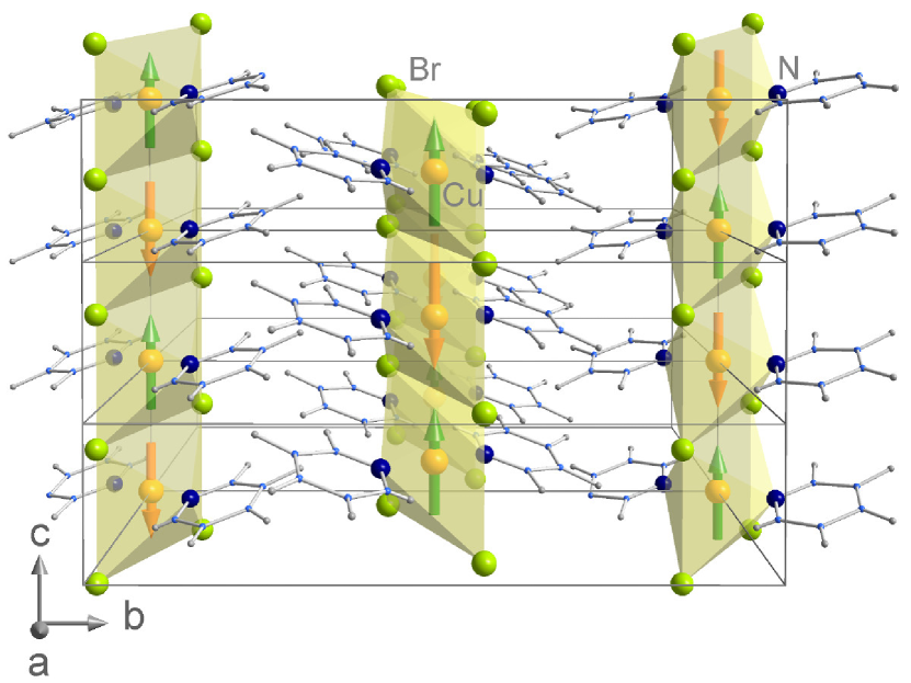
Figure 1: Structure of the compound Cu(py)₂Br₂. Cu ions (yellow), located in the centers of stretched octahedra (Br green, N dark blue), form chains along the $c$ axis which are separated from each other by pyridine rings NC₅H₅ (C light blue, H gray). Crystallographic data are taken from Ref. Morosin, 1975. The arrows indicate the proposed magnetic structure of CPB below $T_{N}\simeq 0.72\,\text{K}$ as discussed in Sec. VI and App. C.

There are two magnetically inequivalent types of chains which differ in the orientation of the stretching axis of the octahedra. They can be transformed into each other by combining a reflection with respect to a plane normal to the $b$ axis lying in between the two chains and a translation of $\bm{c}/2$ in $c$ direction (see Fig. 1). Therefore, the orientation of the ionic $g$-tensors is different for these two chain types, while the $g$-tensors for sites within one chain are identical.

Neighboring magnetic ions in the individual chains are antiferromagnetically coupled by superexchange via the halogen ligands between them. The strength of this intrachain exchange was obtained in Ref. Thede et al., 2012 by comparing the static susceptibility measured in a field along the chain direction with the exact result for the isotropic Heisenberg chain,Johnston et al. (2000) given by Hamiltonian (1) with $\delta=0$. The authors of Ref. Thede et al., 2012 report an isotropic exchange of $J=4.58\,\text{meV}$. Although neighboring chains are well separated from each other, there exists a residual interchain exchange $J^{\prime}$ which leads to 3d ordering at finite temperatures. This transition was observedThede et al. (2012) in specific heat measurements at $T_{N}=0.72\,\text{K}$ and can be used to estimate the strength of the interchain exchange to be $J^{\prime}\approx 0.03\,\text{meV}$ (see e.g. Ref. Yasuda et al., 2005). From these values it follows that the magnetic interactions in CPB have a strong one-dimensional character thus qualifying this compound for comparison with theories based on 1d models like Eq. (1).

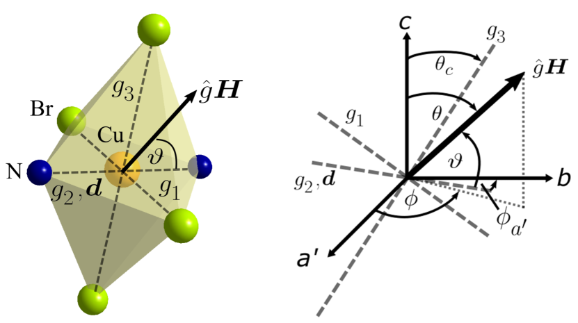
Figure 2: Left: Local coordinate system of a stretched octahedron formed by four bromine ions (green) and two nitrogen ions (dark blue), surrounding the central copper ion (yellow). Principal axes $g_{1}$, $g_{2}$, and $g_{3}$ of the $g$-tensor $\hat{g}$ coincide with the symmetry axes of the stretched octahedron. The angle between local magnetic field $\hat{g}\bm{H}$ and anisotropy axis $\mathbf{d}$ is denoted by $\vartheta$. Right: Angles of $\hat{g}\bm{H}$ ($\theta$, $\phi$), $\mathbf{d}$ ($90^{\circ},90^{\circ}-\phi_{a^{\prime}}$), and $g_{3}$ ($\theta_{c},-\phi_{a^{\prime}}$) with respect to the crystallographic frame $(\mathbf{a}^{\prime},\mathbf{b},\mathbf{c})$. Additionally, the angle $\vartheta$ between $\hat{g}\bm{H}$ and $\mathbf{d}$ is shown.

We measured static magnetization of a CPB sample using a VSM-SQUID magnetometer from Quantum Design Inc. in DC-mode in the temperature range from $1.8\,\text{K}$ to $325\,\text{K}$, in order to reinvestigate the exchange coupling $J$ by taking the effect of a small anisotropy $\delta$ into account.

Beside the pure compound CPB, two doped samples with 2% and 5% Cl content were studied. Their crystal structure is similar to CPB with some of the Br sites occupied by Cl ions, which leads to local changes of the $g$-tensor and of the effective isotropic exchange.Thede et al. (2012) This way disorder is introduced into the system.

For our ESR studies of these compounds two spectrometers were employed. Measurements with a microwave frequency of $9.56\,\text{GHz}$ at temperatures between $3.6\,\text{K}$ and $300\,\text{K}$, and fields up to $0.9\,\text{T}$ were performed using a standard Bruker EMX X-Band spectrometer. HF-ESR was measured using a homemade spectrometer which is described in detail elsewhere.Golze et al. (2006) All HF-ESR measurements were performed in transmission geometry and Faraday configuration, i.e. with wave vector of the microwaves being parallel to the external field.

The neutron diffraction measurements were performed on D23 instrument in Institut Laue-Langevin (Grenoble, France). The fully deuterated sample of CPB was mounted on the dilution refrigerator stick, installed on a standard ILL Orange cryostat. Incident neutron beam with wavelength $\lambda=2.375\,\text{\AA}$ was provided by the PG monochromator. The measurements were performed in a standard geometry with a single ³He detector.

IV Magnetization

The temperature dependence of the magnetization of a CPB sample was measured with a small applied field of about $0.1\,\text{T}$ upon heating after zero field cooling. In one of the measurements the external field was oriented approximately along the chain axis, while in another one it was applied nearly perpendicular to this axis. In the following we neglect small misalignments of the crystal and consider susceptibilities defined as the magnetization divided by the small field of $0.1\,\text{T}$ (see App. A). We label the two susceptibilities and the corresponding data sets by $(\|)$ for $\bm{H}\,\|\,[001]$ and by $(\perp)$ for $\bm{H}\,\perp\,[001]$, respectively. Static susceptibilities extracted from the two measurements are shown in Fig. 3.

For both orientations the behavior of the susceptibility is qualitatively similar, showing a Bonner-Fisher maximum,Bonner and Fisher (1964) which is typical for spin-1/2 chains and whose position and height are mainly related to the strength of the exchange interaction. The fact that the two susceptibility curves differ from each other by a constant factor over a wide temperature range can be mainly attributed to the $g$-factor anisotropy, which can be extracted from the angular dependence of the resonance field of our ESR data at high temperatures (see Sec. V.1), and to geometry factors taking the sample shape into account. The small difference of the positions of the two maxima can be explained by a small anisotropy of the exchange interaction. Assuming the former to be of Ising type we may use first order perturbation theory (see App. A), valid for all temperatures $T\gg J\delta/k_{B}$ with Boltzmann’s constant $k_{B}$, in order to estimate the parameter $\delta$ of Eq. (1).

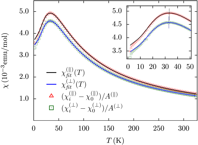
Figure 3: Static susceptibilities of CPB for two orientations of the small magnetic field of 0.1 T ($\|$ and $\perp$ to the $c$ axis) as functions of temperature. Open symbols indicate measured data (minus offsets and divided by geometry factors, see Eqs. (6)). For the sake of clarity, only every sixth of these data points is plotted in the main plot and every second point in the inset. Solid lines show the best fit $\chi_{\text{{fit}}}^{(\|,\perp)}(T)=\chi^{(0)}(T)+\chi_{\text{corr}}^{(\|,\perp)}(T)$, corresponding to $J/k_{B}=52.0\,\text{K}$ and $\delta=-0.019$ (see text). The excellent match between calculated and measured data is emphasized in the inset. Vertical lines indicate the positions of the Bonner-Fisher maxima. The difference in height can be mainly attributed to the $g$-factors of the two field directions.

From the angular dependence of the ESR data in Sec. V.1 we conclude that the anisotropy axes of the spin chains in our material are perpendicular to the $c$ axis. This means that for $\chi^{(\|)}$ the magnetic field is perpendicular to the anisotropy axes. Denoting the magnetic field direction by $z$, the perturbation term becomes $J\delta\sum_{\langle ij\rangle}s_{i}^{x}s_{j}^{x}$, and the first order correction to the isotropic susceptibility, $\chi^{(0)}(T)=g^{2}\mu_{B}^{2}\left\langle s_{1}^{z}\right\rangle_{T,h,0}/h$ with Zeeman energy $h=g\mu_{B}\mu_{0}H$, takes the form (see App. A.2)

$$\chi^{(\|)}_{\text{corr}}(T)=\frac{g^{2}\mu_{B}^{2}J\delta}{h}\frac{\rm d}{{\rm d}h}\left\langle s_{1}^{x}s_{2}^{x}\right\rangle_{T,h,0}\,.$$ (3)

Here, the subscripts at $\left\langle\cdot\right\rangle_{T,h,0}$ mean that the thermal expectation value has to be evaluated with the isotropic Hamiltonian, i.e. Eq. (1) with $\delta=0$, supplemented by the Zeeman term $-hS^{z}=-g\mu_{B}\mu_{0}H\sum_{j}s_{j}^{z}$.

For $\chi^{(\perp)}$ the magnetic field lies in the $a^{\prime}$-$b$ plane. Denoting its direction again by $z$, the anisotropic part of the Hamiltonian of one of the two inequivalent chains in CPB reads

$$\mathcal{H}_{\vartheta}=J\delta\sum_{\langle ij\rangle}(\cos\vartheta\,s_{i}^{z}-\sin\vartheta\,s_{i}^{x})(\cos\vartheta\,s_{j}^{z}-\sin\vartheta\,s_{j}^{x})\,,$$ (4)

where $\vartheta$ is the angle between magnetic field and the corresponding anisotropy axis. If we take into account that the anisotropy axes of the two chains are almost perpendicular to each other, and if we further neglect the small anisotropy of the $g$-factor inside the $a^{\prime}$-$b$ plane (see Sec. V.1), the first order contribution of both chain types to the total susceptibility simplifies to the arithmetic mean of the individual contributions and is therefore given by

$$\chi^{(\perp)}_{\text{corr}}(T)=\frac{g^{2}\mu_{B}^{2}J\delta}{2h}\frac{\rm d}{{\rm d}h}\left\langle s_{1}^{z}s_{2}^{z}+s_{1}^{x}s_{2}^{x}\right\rangle_{T,h,0}\,.$$ (5)

Everything is now reduced to quantities that can be calculated exactly in the thermodynamic limit. The isotropic part $\chi^{(0)}(T)$ of the static susceptibility and its corrections (3) and (5) can be most efficiently computed by solving a simple and finite set of non-linear integral equations arising within the so-called quantum transfer matrix approach to the thermodynamics of integrable lattice models.Klümper (1992, 1993)

We fitted the theoretical predictions

$$\chi^{(\|)}(T) =A^{(\|)}\left(\chi^{(0)}(T)+\chi^{(\|)}_{\text{corr}}(T)\right)+\chi_{0}^{(\|)}\,,$$ (6a)

$$\chi^{(\perp)}(T) =A^{(\perp)}\left(\chi^{(0)}(T)+\chi^{(\perp)}_{\text{corr}}(T)\right)+\chi_{0}^{(\perp)}\,,$$ (6b)

to the measured data $\chi_{i}^{(\|)}$ and $\chi_{i}^{(\perp)}$, respectively. Here, $A^{(\|,\perp)}$ are dimensionless geometry factors and $\chi_{0}^{(\|,\perp)}$ are offsets of the data sets $\chi_{i}^{(\|,\perp)}$ measured in units emu/mol. We derive the general structure of these equations in App. A.1.

The fit values of the isotropic coupling $J$ and the anisotropy parameter $\delta$ depend on the chosen temperature range $[T_{a},T_{b}]$ of the fit. We varied the lower bound $T_{a}$ from $16\,\text{K}$ to $32\,\text{K}$ and the upper bound $T_{b}$ from $200\,\text{K}$ to $325\,\text{K}$. Values of $T_{\text{a}}$ smaller than $22\,\text{K}$ or values of $T_{b}$ larger than $285\,\text{K}$ suddenly decrease the quality of the fit. The former makes sense since a perturbation expansion, as given in Eqs. (6), is only valid for $T\gg J\delta/k_{B}\approx 1\,\text{K}$. The latter is due to more noise and perhaps a systematic error in the susceptibility data above room temperature. The best fit is obtained for $T_{a}=23.5\,\text{K}$ and $T_{b}=285\,\text{K}$ and yields

$$J/k_{B} =52.0\,\text{K}\pm 0.1\,\text{K}\,,$$ (7)

$$\delta =-0.019\pm 0.002\approx-0.02\,.$$ (8)

Offsets and prefactors are $\chi_{0}^{(\|)}=1.46\cdot 10^{-4}\,\text{emu}/\text{mol}$, $\chi_{0}^{(\perp)}=-2.77\cdot 10^{-4}\,\text{emu}/\text{mol}$ and $A^{(\|)}\cdot(g^{(\|)})^{2}=4.48$, $A^{(\perp)}\cdot(g^{(\perp)})^{2}=4.55$, respectively. If we set $g^{(\|)}=g_{c}=2.154$ and $g^{(\perp)}\approx 2.069$ as obtained by means of ESR spectroscopy in Sec. V, the latter value being an estimated average over $g$-values in the $a^{\prime}$-$b$ plane, both geometry factors are close to one, $A^{(\|)}=0.97$, $A^{(\perp)}=1.06$.

Figure 3 shows the data sets $(\chi_{i}^{(\|,\perp)}-\chi^{(\|,\perp)}_{0})/A^{(\|,\perp)}$ together with the two curves $\chi^{(0)}(T)+\chi_{\text{corr}}^{(\|,\perp)}(T)$ of the best fit with $\delta=-0.019$ and $J/k_{B}=52.0\,\text{K}$. The fit provides a reliable estimate of the anisotropy in CPB (for details see App. A). The relative positions of the two maxima (see inset of Fig. 3) already give a clear hint at the sign of $\delta$. The fact that the position of the maximum of $\chi^{(\|)}(T)$ is slightly shifted to higher temperatures as compared to the one of $\chi^{(\perp)}(T)$ implies that the anisotropy is negative and small (see Eq. (42) in App. A.2) meaning that the Hamiltonian is critical in zero magnetic field.

In the low-temperature regime $T\leq 3\,\text{K}$ our susceptibility data show a strong decrease with decreasing temperatures and the curves obtained from a perturbation expansion in $\delta$ deviate from the experimental data (see inset of Fig. 3). This is compatible with the fact that the perturbation expansion is only valid for $T\gg J\delta/k_{B}\approx 1\,\text{K}$. The low-temperature behavior might be qualitatively explained by an effective magnetic excitation gap which opens if the applied field is perpendicular to the anisotropy axisHieida et al. (2001); Dmitriev et al. (2002) or by the proximity of the 3d antiferromagnetic phase transition at $T_{N}\approx 0.72\,\text{K}$.

V ESR on Cu(py)₂Br₂

V.1 Angular dependence of ESR parameters

We study the angular dependence of the ESR spectrum of CPB at room temperature and for a fixed frequency of $\nu=9.56\,\text{GHz}$. We recorded three data sets. For two of them the $c$ axis of the sample was initially aligned with the external field, then rotated away from the field direction by $90^{\circ}$. A third data set pertains to a rotation about the $c$ axis which enclosed an angle of $90^{\circ}$ with the external field. This data set corresponds to a rotation of the field in the $a^{\prime}$-$b$ plane in the reference frame of the sample. In Fig. 2 we show the local octahedral environment of the Cu²⁺ ions of one of the two inequivalent chains and its relative position to the crystallographic frame $(\mathbf{a}^{\prime},\mathbf{b},\mathbf{c})$.

All recorded spectra show single spectral lines from which we extracted the resonance fields $\mkern 4.7mu\overline{\mkern-4.7muH\mkern-1.5mu}\mkern 1.5mu$ and linewidths $\mkern 2.5mu\overline{\mkern-2.5muw\mkern-0.8mu}\mkern 0.8mu$ as functions of the rotation angle $\alpha$. The corresponding curves of ESR parameters are shown in Figs. 4 and 5 as black squares.

It turns out that the analysis of these curves is rather intricate. This is first of all due to the fact that we are dealing with two inequivalent chains (see Fig. 1) meaning that we have to interpret the recorded spectral lines as superpositions of two individual lines which are so close to each other that they are not resolved at the applied frequency. Note that in principle —besides the exchange narrowing effect due to intrachain interaction given by $J$— there might be an additional exchange narrowing effect caused by interchain interactions $J^{\prime}$, which would lead to the fusion of the two spectral lines.Pal et al. (1994); Hennessy et al. (1973) Such effect might be anticipated from the fact that in case of CPB $J^{\prime}$ is larger than the difference in Zeeman energies of the inequivalent chains. However, angular dependencies of ESR parameters of the resulting single line are not compatible with our results obtained by rotation of magnetic field in a-b-plane, which can be described only in terms of contributions from two individual lines, see below.

A second difficulty arising in the analysis of our data comes from the fact that the octahedra surrounding the magnetically active Cu²⁺ ions are distorted in such a way that the cubic symmetry of the undistorted octahedra is fully broken. This implies that we are dealing with the most general possible g-tensor which, as a symmetric rank two tensor, depends on six independent parameters, e.g. its eigenvalues $g_{1},g_{2},g_{3}$ and three angles fixing its orientation in space. We may therefore write it as

$$\hat{g}=D\operatorname{diag}(g_{1},g_{2},g_{3})D^{t}\,,$$ (9)

where $D$ is the rotation matrix transforming the principle coordinate system of the $g$-tensor into the crystallographic frame $(\mathbf{a}^{\prime},\mathbf{b},\mathbf{c})$. The $g$-factor anisotropy is caused by spin-orbit coupling which mixes, in the case of Cu²⁺ ions, some of the $t_{2g}$ states to the ground state, i.e. the $d_{x^{2}-y^{2}}$ state.Abragam and Bleaney (2012) Since the anisotropy is small we expect a close-to-isotropic $g$-tensor, i.e. $g_{1}\approx g_{2}\approx g_{3}$.

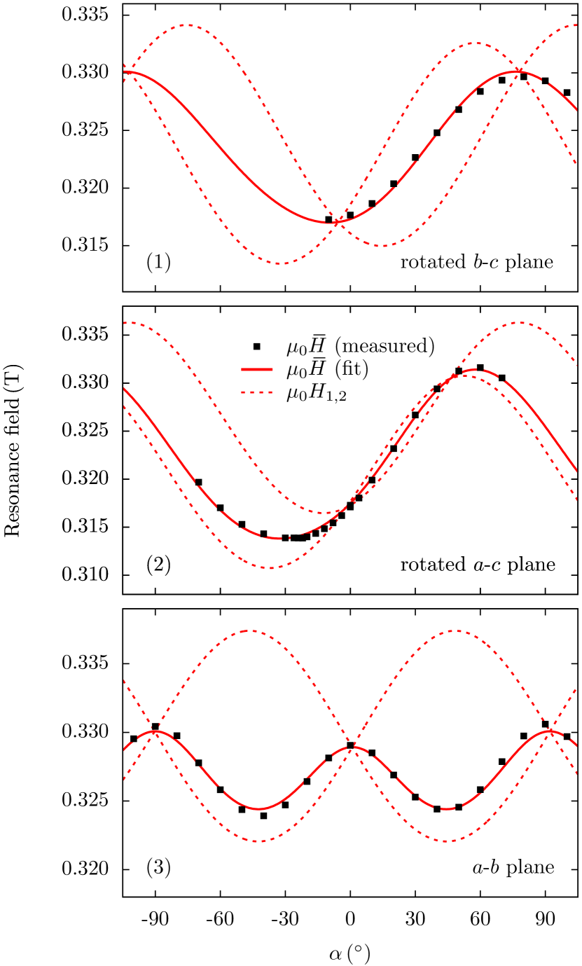
Figure 4: Angular dependence of the measured resonance field for CPB (dots) at frequency $\nu=9.56\,\text{GHz}$ and at room temperature for rotation of the magnetic field in planes containing the $c$ axis (top and middle) and in the $a^{\prime}$-$b$ plane (bottom), compared to the fitted theoretical curves $\mu_{0}\mkern 4.7mu\overline{\mkern-4.7muH\mkern-1.5mu}\mkern 1.5mu$ (solid lines). Dashed lines indicate the resonance fields $\mu_{0}H_{1,2}$ of the two individual, unresolved lines (see Eq. (13) and text).

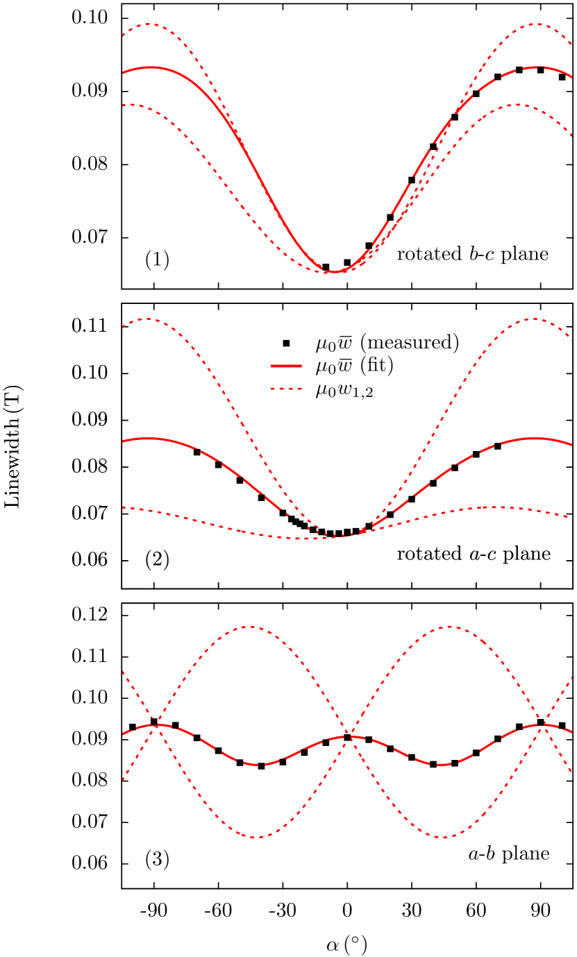
Figure 5: Angular dependence of the measured ESR linewidth for CPB (dots) at frequency $\nu=9.56\,\text{GHz}$ and at room temperature for rotation of the magnetic field in planes containing the $c$ axis (top and middle) and in the $a^{\prime}$-$b$ plane (bottom), compared to the fitted theoretical curves $\mu_{0}\mkern 2.5mu\overline{\mkern-2.5muw\mkern-0.8mu}\mkern 0.8mu$ (solid lines). Dashed lines indicate the linewidths $\mu_{0}w_{1}$ and $\mu_{0}w_{2}$ of the two individual, unresolved lines (see Eq. (14) and text).

We analyze the angular dependence of the ESR parameters based on the model of two non-interacting inequivalent XXZ chains. In the following, we denote Bohr’s magneton by $\mu_{B}$, the permeability of free space by $\mu_{0}$, and Planck’s constant by $2\pi\hbar$. The letter $h$ is already used as abbreviation for the Zeeman energy $h=g\mu_{B}\mu_{0}H$ and should not be confused with Planck’s constant. For a single chain our theory relies on perturbation theory in $\delta$, on an analysis of the moments of the shape function, and on a high-temperature expansion in $J/(k_{B}T)$ for the resonance shift $s(\delta)$ and the linewidth $w$ (see App. B.1). The resonance shift is related to the resonance field $H$ by

$$H=\frac{\hbar\omega-Js(\delta)}{g\mu_{B}\mu_{0}}\,.$$ (10)

Here, $\nu=\omega/(2\pi)$ is the frequency of the incident microwaves and $g=\|\hat{g}\mathbf{e}\|$, where $\mathbf{e}$ is the unit vector in the direction of the external magnetic field. To leading order in $J/(k_{B}T)$ we obtain the following expression for the resonance shift (see Eq. (58b) of App. B.1),

$$s(\delta)=\frac{J\delta}{4k_{B}T}\left[(1-3\cos^{2}\vartheta)\frac{\hbar\omega}{J}+(1+\cos^{2}\vartheta)\frac{\delta}{2}\right]$$ (11)

with $\vartheta$ being the angle between the magnetic field direction $\hat{g}\mathbf{e}/g$ at the Cu sites and the anisotropy axis of the chain. Note that up to first order in $\delta$ the frequency term $\hbar\omega$ can be replaced by $g\mu_{B}\mu_{0}H$. This relation will be also proven useful for the analysis of high-frequency ESR measurements at high temperatures in the next section.

In 1d systems the usual exchange narrowing argument fails. It can be replaced by a modified argument, leading to ‘inhibited exchange narrowing’.Hennessy et al. (1973) Further elaborating on this idea we derive a novel formula for the linewidth for small $\delta$ and in the high-temperature regime (see App. B.1),

$$w\approx\frac{AJ}{g\mu_{B}\mu_{0}}\left[\frac{\delta^{2}}{4}(1+\cos^{2}\vartheta)\right]^{\beta}\,.$$ (12)

The proportionality factor $A$ is unknown and should be of order one. As explained in App. B.1, the exponent $\beta$ is connected with the decay of a certain time-dependent correlation function in the isotropic system at high temperature.

Eqs. (10), (11) and (12) determine the resonance field and linewidth of the absorption spectrum of a single XXZ chain with small anisotropy and in the high-temperature regime. We still have to take into account that the observed spectra must be interpreted as the superposition of the spectra of two types of chains, type 1 and type 2, which are distinguished by the orientation of their $g$-tensors and anisotropy axes. We shall assume for simplicity that in its center each of the two spectral lines can be approximated by a Lorentzian and that the two lines have equal spectral weight. For two equally normalized Lorentzians with maxima at $H_{1}$, $H_{2}$ and widths $w_{1}$, $w_{2}$ their sum is well approximated again by a Lorentzian if only $|H_{1}-H_{2}|\ll\text{min}\{w_{1},w_{2}\}$. The location of the maximum of the resulting line is approximated by

$$\mkern 4.7mu\overline{\mkern-4.7muH\mkern-1.5mu}\mkern 1.5mu=\frac{H_{1}w_{1}^{-3}+H_{2}w_{2}^{-3}}{w_{1}^{-3}+w_{2}^{-3}}+\mathcal{O}(\epsilon_{H}^{3}\epsilon_{w})$$ (13)

and its width $\mkern 2.5mu\overline{\mkern-2.5muw\mkern-0.8mu}\mkern 0.8mu$ can be expressed as

$$\mkern 2.5mu\overline{\mkern-2.5muw\mkern-0.8mu}\mkern 0.8mu =\sqrt{\sqrt{w_{1}^{2}w_{2}^{2}+\frac{(w_{1}-w_{2})^{4}}{4}}-\frac{(w_{1}-w_{2})^{2}}{2}}$$

$$\quad\,+\frac{(H_{1}-H_{2})^{2}}{w_{1}+w_{2}}\left(\frac{3}{4}-\frac{25}{8}\left(\frac{w_{1}-w_{2}}{w_{1}+w_{2}}\right)^{2}\right)$$

$$\quad\,+\mathcal{O}(\epsilon_{H}^{3},\epsilon_{H}^{2}\epsilon_{w}^{4})$$ (14)

with small numbers $\epsilon_{w}=(w_{1}-w_{2})/(w_{1}+w_{2})$ and $\epsilon_{H}=(H_{1}-H_{2})/(w_{1}+w_{2})$. The formula for the location $\mkern 4.7mu\overline{\mkern-4.7muH\mkern-1.5mu}\mkern 1.5mu$ of the maximum represents a weighted mean of the two resonance fields $H_{1}$ and $H_{2}$ with weights $1/w_{1,2}^{3}$. Note that it holds for other line shapes than Lorentzians, e.g. for a superposition of two Gaussians, too. The first line in expression (14) for the resulting width $\mkern 2.5mu\overline{\mkern-2.5muw\mkern-0.8mu}\mkern 0.8mu$ can be understood as a modified geometric mean of two individual widths $w_{1}$ and $w_{2}$, whereas the second line reflects an additional broadening caused by the finite distance of the maxima positions.

We fit derivatives of Lorentzians to the measured spectral lines as, due to the use of lock-in techniques, the derivative of the absorption line was recorded in our low-frequency ESR experiments. We identify Lorentz parameters ‘position’ and ‘width’ with $\mkern 4.7mu\overline{\mkern-4.7muH\mkern-1.5mu}\mkern 1.5mu$ and $\mkern 2.5mu\overline{\mkern-2.5muw\mkern-0.8mu}\mkern 0.8mu$ of Eqs. (13) and (14), respectively. For the individual resonance shifts $H_{1}$, $H_{2}$ and linewidths $w_{1}$, $w_{2}$ of the two types of lines we have used Eqs. (10) and (12) with the respective orientations of the $g$-tensors and anisotropy axes. Taking these equations as they are, the number of parameters to be determined would be too large for a stable fit. Ideally the following parameters of the model should be extracted from a fit: the anisotropy $\delta$, the eigenvalues $g_{1}$, $g_{2}$, $g_{3}$ of the $g$-tensor, $2\times 3$ angles fixing the rotation matrices $D_{1}$ and $D_{2}$ that determine the orientation of the $g$-tensors of the two types of chains, $2\times 2$ angles fixing two unit vectors $\mathbf{d}_{1}$, $\mathbf{d}_{2}$ defining the direction of the anisotropy axes of the two types of chains, and finally the parameters $A$ and $\beta$ entering Eq. (12).

In order to reduce the number of unknowns of the fit, we fix the ‘geometric parameters’ $D_{1}$, $D_{2}$ and $\mathbf{d}_{1}$, $\mathbf{d}_{2}$ by resorting to the crystal structure (see Sec. III) and by inspecting the qualitative behavior of the data. We have seen in Sec. III that the two inequivalent chains in CPB are related by a glide reflection with reflection component $R=\operatorname{diag}(1,-1,1)$ representing a reflection at the $a$-$c$ plane. This implies that $RD_{1}=D_{2}R$ and $R\mathbf{d}_{1}=\mathbf{d}_{2}$, i.e. $g$-tensors and anisotropy axes of the two chains must be related by this reflection. It is convenient to specify the direction $\mathbf{e}$ of the external magnetic field in terms of spherical coordinates $\theta$, $\phi$ with respect to the crystallographic frame $(\mathbf{a}^{\prime},\mathbf{b},\mathbf{c})$. Then, $\mathbf{e}=\mathbf{e}(\theta,\phi)$ and the $g$-factors $g_{j}=\|\hat{g}_{j}\mathbf{e}\|$, $j=1,2$, of the two chains become functions of $\theta$ and $\phi$. Eq. (9) implies that $g_{j}(\theta,\phi)$ is periodic in $\theta$ with period $180^{\circ}$, that $g_{j}(0,\phi)$ is periodic in $\phi$, also with period $180^{\circ}$, and that $g_{2}(\theta,\phi)=g_{1}(\theta,-\phi)$.

The most striking feature of the experimental resonance shift and linewidth shown in Figs. 4 and 5 is that they exhibit a $180^{\circ}$ periodicity if the field is rotated in planes perpendicular to the $a^{\prime}$-$b$ plane, but a $90^{\circ}$ periodicity if the field is rotated within the $a^{\prime}$-$b$ plane. The $g$-factors of the individual chains have a periodicity of $180^{\circ}$ for all rotation directions. The periods of resonance field and linewidth induced by the anisotropy of the individual chains are $180^{\circ}$, too, as can be seen from Eqs. (11), (12). Thus, any shorter period or modulation must come from the superposition of the resonance lines of the two chains.

Let us first consider the variation of the linewidth (see Eqs. (12) and (14) as well as Fig. 5). In Eq. (12) the variation of the $g$-factor with the external field is a subleading effect, the main variation of the width coming from the variation of $\vartheta$. In the upper two panels of Fig. 5 no modulation of the $180^{\circ}$ periodicity is visible, showing that both angles $\vartheta_{1}$ and $\vartheta_{2}$ and thus both individual widths $w_{1}$ and $w_{2}$ have the same monotonic behavior as function of rotation angle $\alpha$. By contrast, the $90^{\circ}$ modulation of the width in the lower panel points towards a phase difference of about $90^{\circ}$ between $\vartheta_{1}$ and $\vartheta_{2}$. This can be understood if the anisotropy axes lie in the $a^{\prime}$-$b$ plane and are almost perpendicular to each other. Taking into account that $R\mathbf{d}_{1}=\mathbf{d}_{2}$, they should enclose an angle of about $45^{\circ}$ with the $a^{\prime}$ axis. Thus, the anisotropy axis should either be directed along the projection of the stretched octahedron axes onto the $a^{\prime}$-$b$ plane or perpendicular to this direction. Only the latter case is (approximately) in accordance with the reflection symmetries of the deformed octahedra. For this reason we conclude that the anisotropy axes of the chains are located in the $a^{\prime}$-$b$ plane and enclose angles $\pm(90^{\circ}-\phi_{a^{\prime}})=\pm 46.56^{\circ}$ with the $a^{\prime}$ axis. As we shall see this will also explain the behavior of the resonance field, Eqs. (10) and (11), if the $g$-tensor anisotropy is properly taken into account.

For the $g$-tensor anisotropy we hypothesize that it is entirely due to the deformation of the octahedra formed by the Br and N atoms surrounding the magnetically active Cu²⁺ spin. Then, the $g$-tensor should be diagonal in a coordinate system symmetrically attached to the deformed octahedra. Denoting by $D(\alpha,\mathbf{n})$ the matrix for a rotation about an axis $\mathbf{n}$ by an angle $\alpha$, we are setting

$$D_{1} =D(\phi_{a^{\prime}},\mathbf{c})D(-\theta_{c},\mathbf{b})\,,$$ (15a)

$$D_{2} =D(-\phi_{a^{\prime}},\mathbf{c})D(-\theta_{c},\mathbf{b})\,,$$ (15b)

which means that we are neglecting the small declination away from the $a^{\prime}$-$b$ plane of the line connecting the nitrogen atoms in the octahedron (see Sec. III and Fig. 2). The above notation is also useful to represent $\mathbf{d}_{1}$ and $\mathbf{d}_{2}$ explicitly as

$$\mathbf{d}_{1,2}=D(\pm\phi_{a^{\prime}},\mathbf{c})\mathbf{b}=D(\pm(90^{\circ}-\phi_{a^{\prime}}),\mathbf{c})\mathbf{a}^{\prime}\,,$$ (16)

which means that the anisotropy axis of each chain coincides with the connecting line of the two nitrogen ions (see Fig. 2).

Presuming Eqs. (15) and (16) we have reduced the model parameters to be fitted to the angular dependence of the high-temperature ESR data to $\delta$, $g_{1}$, $g_{2}$, $g_{3}$, $A$, and $\beta$. We reduce the number of these parameters further by using $\delta=-0.019$ as obtained from our susceptibility measurements. Except for these model parameters we also have to determine some experimental parameters connected with the limited control over the sample position during our measurements, which are described below.

The best fit yields for the remaining model parameters

$$(g_{1},g_{2},g_{3}) =(2.065,\,2.018,\,2.203)\,,$$ (17)

$$A =1.3\,,$$ (18)

$$\beta =0.77\,.$$ (19)

The estimated error of $\beta$ is about $3\,\%$ and those of the three $g$-values $g_{1,2,3}$ are less than $0.5\,\%$. The three values of $g_{1,2,3}$ in Eq. (17) together with Eqs. (15) determine the full $g$-tensor for both chain types and are typical for Cu²⁺ ions in an octahedral environment.Abragam and Bleaney (2012) For a magnetic field applied along the chain axes, the $g$-factors of both chain types are the same due to reflection symmetry and take the value $g_{c}=2.154$. This value is in excellent agreement with the value obtained independently from high-frequency measurements (see Sec. V.2 below).

For a different choice of the model parameter $\delta$, say $\delta=-0.01$, $-0.03$, or $-0.05$, the best fit yields similar values of $g_{1}$ and $g_{3}$ as well as of $\beta$, all lying in the estimated error intervals. This can be understood by the observation that the effect of $\delta$ on the resonance position at high temperatures in Eq. (10) is very small: $s(\delta)\sim\delta/T$. The variation of the fit parameter $g_{2}$ with $\delta$ is slightly larger (up to $1.5\,\%$), leading to values $g_{2}\leq 2$ for $\delta<-0.04$. Furthermore, the model parameter $\delta$ enters the formula of the linewidth, Eq. (12), via the prefactor $A\cdot\delta^{2\beta}$. If $\delta$ was too small in absolute value this would yield values of $A$ not of order one, in contradiction to our expectation (see App. B.1). This way and by demanding that $g_{2}>2$ we can exclude values of $\delta$ greater than $-0.01$ and less than $-0.04$, in agreement with our previous findings.

Except for the model parameters the fit yields a number of experimental parameters, for instance ‘off-plane’ angles $\phi_{\text{op}}^{(1,2)}$ and $\theta_{\text{op}}^{(a^{\prime}b)}$. The former are angles between the $b$-$c$ plane (label 1) or the $a$-$c$ plane (label 2) and planes rotated about the $c$ axis by $\phi_{\text{op}}^{(1,2)}$. Their meaning is that during the corresponding measurement (labels (1) and (2) in Figs. 4 and 5) the crystal was rotated such that the external magnetic field was lying in these rotated planes rather than in the unrotated $b$-$c$ or $a$-$c$ planes. During the rotation of the third measurement (label (3) in Figs. 4 and 5) the $a^{\prime}$-$b$ plane enclosed an angle $\theta_{\text{op}}^{(a^{\prime}b)}$ with the external magnetic field. Since $\theta_{\text{op}}^{(a^{\prime}b)}$ is small (see below) we can neglect it and call this a rotation of the magnetic field inside the $a^{\prime}$-$b$ plane. Further, offset angles $\alpha_{\text{os}}^{(1,2,a^{\prime}b)}$ are determined by the fit. They describe (small) misalignments of the external magnetic field with crystallographic axes, e.g. the $c$ axis for measurements (1) and (2) or the $a^{\prime}$ axis for measurement (3), at $\alpha=0$. They read

$$(\phi_{\text{op}}^{(1)},\phi_{\text{op}}^{(2)},\theta_{\text{op}}^{(a^{\prime}b)}) =(-6.4^{\circ},\,26.9^{\circ},\,1.2^{\circ})\,,$$ (20)

$$(\alpha_{\text{os}}^{(1)},\alpha_{\text{os}}^{(2)},\alpha_{\text{os}}^{(a^{\prime}b)}) =(5.6^{\circ},\,1.9^{\circ},\,-0.9^{\circ})\,.$$ (21)

The values of $\theta_{\text{op}}^{(a^{\prime}b)}$, $\alpha_{\text{os}}^{(2)}$, and $\alpha_{\text{os}}^{(a^{\prime}b)}$ are negligible. The order of magnitude of $\alpha_{\text{os}}^{(1)}\sim 5^{\circ}-10^{\circ}$ could have been already estimated by eye from the corresponding data sets of the upper panels of Figs. 4 and 5.

Figures 4 and 5 show the experimental data (black dots) together with the fitted theoretical curves (red solid lines) for the angular dependence of resonance position and linewidth. The red dashed lines represent the contributions from the two inequivalent chains. The linewidth, measured as width at half height, of the sum of a broad and a narrow line is dominated by the width of the narrow line. In all cases we assume equal intensities of the two lines composing the observed spectral line. Therefore, the width of the observed line is minimal if the linewidth of one of the two contributing lines has a minimum (see lower panel of Fig. 5). From our point of view the agreement of the fitted curves $\mkern 4.7mu\overline{\mkern-4.7muH\mkern-1.5mu}\mkern 1.5mu(\alpha)$ and $\mkern 2.5mu\overline{\mkern-2.5muw\mkern-0.8mu}\mkern 0.8mu(\alpha)$ with the measured data points is rather convincing in all three cases.

In conclusion, from the angular dependence of the ESR parameters measured at room temperature $T\gg J/k_{B}\approx 52.0\,\text{K}$, the eigenvalues of the $g$-tensor could be determined. The scenario of two anisotropy axes in the $a^{\prime}$-$b$ plane explains the observed angular dependence of resonance field and linewidth. Furthermore, from heuristic arguments the possible value of $\delta$ could be restricted to the interval $[-0.04,-0.01]$ which is compatible with the value of $\delta=-0.019$ obtained from susceptibility measurements. Additionally, the values of $A$ and $\beta$ in Eq. (12) could be estimated. We expect that, due to further progress in theory, they may be calculated one day. For the time being they provide experimentally measured quantities of certain time-dependent correlation functions of the isotropic Heisenberg chain. The value of $\beta=0.77$, for instance, is related to the algebraic long-time decay of the finite-temperature correlation function ($T\approx 6J/k_{B}$) that appears under the integral of Eq. (56c) (see Eqs. (63)-(65) in App. B, valid at high temperatures).

In the infinite temperature limit this correlation function simplifies to

$$g_{\infty}(t) =\frac{4}{2^{L}L}\sum_{j,k=1}^{L}\text{Tr}\Big{\{}e^{iH_{\text{xxx}}t}s_{j}^{+}s_{j+1}^{+}e^{-iH_{\text{xxx}}t}s_{k}^{-}s_{k+1}^{-}\Big{\}}$$

$$\simeq\alpha(Jt)^{-\gamma_{\infty}}$$ (22)

with $\gamma_{\infty}=0.6$, i.e. $\beta_{\infty}=0.71$ (see App. B.3). The value of $\beta=0.77$, i.e. $\gamma=0.70$, at $T\approx 6J/k_{B}$ is in accordance with a numerical analysis that we performed for finite temperatures, $1\leq k_{B}T/J\leq 100$, and up to $28$ lattice sites, similar to the one in App. B.3 for infinite temperature (see e.g. Fig. 12).

V.2 Frequency dependence of the resonance position

We conducted HF-ESR studies of the resonance shift of the spectral line for comparison with calculations presented in Refs. Oshikawa and Affleck, 2002, Maeda et al., 2005 and Refs. Brockmann et al., 2011, Brockmann et al., 2012. Measurements of the frequency dependence of the ESR parameters were performed at $4\,\text{K}$ and $300\,\text{K}$ in a frequency range from $50\,\text{GHz}$ to $325\,\text{GHz}$ on a sample which was oriented such that $\bm{H}\,||\,[001]$. The results for the resonance positions at both temperatures are shown in Fig. 6.

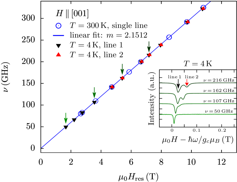
Figure 6: Frequency-field dependence of resonance positions for CPB at $300\,\text{K}$ and $4\,\text{K}$ with external magnetic field oriented along the $c$ axis. Arrows in the main plot indicate the resonance positions of the selected ESR spectra shown in the inset, recorded at $4\,\text{K}$ and, for a better comparison, shifted horizontally by the paramagnetic resonance frequency as well as vertically by arbitrary amounts.

In paramagnets the resonance field and the absorption frequency of spins probed in ESR experiments are linear functions of each other. In the presence of spin-orbit coupling the resonating spin is sensitive to the crystal field of its paramagnetic environment whose reaction to an external magnetic field is then encoded in the (ionic) $g$-tensor. Antiferromagnetic exchange coupling between neighboring spins induces an additional shift of the resonance position, which is a pure many-body effect and depends on the exchange anisotropy, quantified by $\delta$ in our case. In theory it is easy and natural to distinguish between the effect of the $g$-tensor and the (many-body) resonance shift $s(\delta)$, see Eq. (10). In experiments, however, it may be difficult to separate the two effects, because $s(\delta)$ depends linearly on the field for small fields. In Refs. Brockmann et al., 2011, 2012 some of us derived a formula that allows to compute the resonance shift at arbitrary temperature for a single XXZ chain with the magnetic field applied in the direction of the anisotropy axis. A strong deviation from the linear behavior for large enough magnetic fields ($h/J\gtrsim 0.1$) and not too small anisotropy (e.g. $\delta\approx-0.1$) of the model Hamiltonian (1) was found. However, it turned out that the anisotropy of CPB is too small and that the magnetic fields realizable in our experiments are not strong enough to find a pronounced deviation from the linear behavior.

Still, a careful analysis of our data allows us to extract the resonance shift at high and low temperatures. From the analysis of the ESR data recorded at high-temperature and with an external field in $c$ direction we obtain, based on Eq. (11) with $\vartheta=90^{\circ}$, an estimate of the $g$-value $g_{c}$. The shift at high temperatures is small and proportional to the resonance field itself. Therefore, it can be absorbed into the proportionality factor denoted by $m$ in Eq. (24), which is sometimes called an ‘effective $g$-factor’. The temperature independent value $g_{c}$ can then be obtained by fitting a straight line to the resonance position measured at high temperatures, and taking the first order high-temperature correction into account. Furthermore, higher corrections imply a way to estimate the magnitude of $\delta$.

At low temperature the resonance shift as a function of the resonance field shows stronger deviation from linear behavior. Fitting different theoretical predictionsOshikawa and Affleck (2002); Maeda et al. (2005); Brockmann et al. (2011, 2012) we shall obtain two more estimates of the anisotropy parameter $\delta$. Both of them are compatible with our previously obtained values within the estimated errors.

Another approachPsaroudaki et al. (2014) that works for small system sizes at zero temperature is based on Bethe ansatz techniques and identifies a certain excited state above the ground state that contributes most (as compared to all other states, at least for small system sizes) to the ESR absorption spectrum. We computed the difference of the energy of this state to the ground state energy for different magnetic fields up to system size $L=256$ by means of Bethe ansatz. The dependence of this energy difference on the magnetic field agrees well with the corresponding resonance shifts of the measured spectra at low temperatures for all used frequencies and is in accordance with field theory and the moment-based approach considered in more detail below.

V.2.1 High temperatures

At $T=300\,\text{K}$ we observed single resonance lines which show a linear frequency-field relation (see Fig. 6). In the high-temperature regime and for small anisotropies, the resonance condition for the frequency $\nu=\omega/(2\pi)$ of the incident microwave and the resonance field $H_{\text{res}}$ reads (see Eqs. (10) and (11) with $\vartheta=90^{\circ}$)

$$\frac{\hbar\omega}{J}=g_{c}\left(1+\frac{J\delta}{4k_{B}T}\right)\frac{\mu_{B}\mu_{0}H_{\text{res}}}{J}+\frac{J\delta^{2}}{8k_{B}T}\,.$$ (23)

This explicit expression is deduced from a perturbation expansion in $\delta$ up to second order and a high-temperature expansion up to $J/(k_{B}T)$ of the shifted moment $m_{1}$, cf. Eqs. (52), (54b) and (58b). We fit the function $y=mx+b$ with dimensionless quantities $y=\hbar\omega/J$ and $x=\mu_{B}\mu_{0}H_{\text{res}}/J$ to the high-temperature data and obtain

$$m =g_{c}\left(1+\frac{J\delta}{4k_{B}T}\right)=2.1512\,,$$ (24)

$$b =\frac{J\delta^{2}}{8k_{B}T}=5\cdot 10^{-6}\,.$$ (25)

Setting $J/k_{B}=52.0\,\text{K}$ and $T=300\,\text{K}$, Eq. (25) provides an estimate of the magnitude of the anisotropy, $|\delta|\approx 0.015$. We would like to point out, however, that the error of $b$ is larger than $b$ itself, implying that the estimate of $|\delta|$ from Eq. (25) is not reliable. This is mainly due to the fact that the anisotropy $\delta$ of CPB is small and that the $y$ axis intercept $b$ is proportional to $\delta^{2}$. However, at least an upper bound of the order of magnitude can be estimated and agrees well with previous findings of $\delta$. For other materials with larger anisotropy this method would provide a way to estimate $\delta$ with a smaller relative error.

We still use this value of $\delta$ to estimate the $g$-factor $g_{c}$ in $c$ direction from Eq. (24), since previously obtained more reliable values, e.g. $\delta=-0.019$, are close enough to $\delta=-0.015$. Within the fit error of $m$, which is less than $0.1\,\%$, these more reliable values would result in the same value of $g_{c}=2.153$. This $g$-value, in turn, is in excellent agreement with $g_{c}=2.154$ obtained in the previous section by fitting to angular-dependent data.

V.2.2 Low temperatures

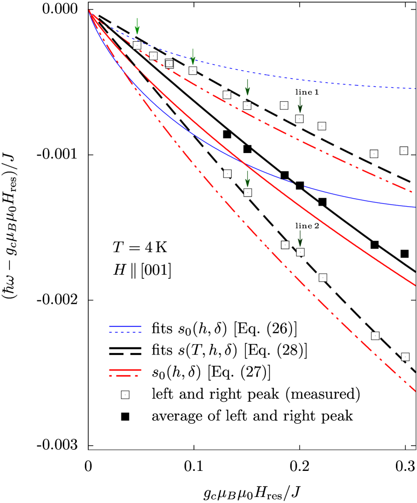
Figure 7: Resonance shift for CPB at $4\,\text{K}$ with magnetic field oriented along the $c$ axis, calculated from resonance positions presented in Fig. 6. Experimental data (squares) are compared with different theoretical predictions (solid lines for the averaged shift, dashed lines for the shifts of line 1 and line 2). Frequencies and resonance fields are rendered dimensionless by multiplying with $\hbar/J$ and $g_{c}\mu_{B}\mu_{0}/J$ (with temperature independent $g_{c}=2.153$; see Sec. V.2.1). Arrows indicate the shifts of the exemplary spectra shown in the inset of Fig. 6.

The temperature-independent value of $g_{c}=2.153$ can be used in the analysis of the resonance shift at low temperatures. Spectra recorded at $4\,\text{K}$ consist of a resonance line (line 1 in the inset of Fig. 6) present at all frequencies and a second line (line 2) which evolves for higher frequencies and is clearly visible above $141\,\text{GHz}$. Both lines show an almost linear frequency-field dependence. The deviations from a straight line can be attributed to the resonance shift, which is shown in Fig. 7.

We compare three theoretical predictions for the resonance shift at low temperatures, $T\ll J/k_{B}$, with the experimentally observed data at $T=4\,\text{K}$ (black squares in Fig. 7). To this end, we subtract the dimensionless resonance fields $h/J=g_{c}\mu_{B}\mu_{0}H_{\text{res}}/J$ from the corresponding dimensionless frequencies $2\pi\hbar\nu/J=\hbar\omega/J$. The result defines the dimensionless ESR resonance shift $s(T,h,\delta)$.

The first prediction for the shift $s(T,h,\delta)$ was obtained by Oshikawa and Affleck within a field theoretical approachOshikawa and Affleck (2002) (blue lines in Fig. 7). It is supposed to hold for $T\rightarrow 0$ and reads

$$s_{0}(h,\delta):=\lim_{T\to 0}s(T,h,\delta)\simeq\frac{h\delta}{J\pi^{2}}\ln\left(\frac{J}{h}\right)\,.$$ (26)

The second prediction (red lines in Fig. 7) is due to Maeda, Sakai, and Oshikawa.Maeda et al. (2005) It extends Eq. (26) to larger resonance fields as it includes logarithmic corrections to field theory,

$$s_{0}(h,\delta)=\frac{h\delta}{J\pi^{2}}\left\{\mathcal{L}+\frac{\ln(\mathcal{L})}{2}+\frac{3}{2}+\frac{1+\ln(\mathcal{L})}{4\mathcal{L}}\right\}$$ (27)

with $\mathcal{L}=\ln[2J\sqrt{\pi^{3}}/(h\sqrt{2e})]$. This equation was derived from the finite temperature result of Ref. Maeda et al., 2005 (extended to arbitrary anisotropy in Ref. Brockmann et al., 2011) by taking the zero temperature limit and expanding for small Zeeman energies $h$. In this work we use a different definition of the resonance shift (see App. B.1) as compared to Refs. Maeda et al., 2005 and Brockmann et al., 2011. Up to first order in $\delta$, however, the resonance shift at finite temperature is determined by the same combination of static correlation functions,

$$s(T,h,\delta)=\delta\frac{\left\langle s_{1}^{z}s_{2}^{z}-s_{1}^{x}s_{2}^{x}\right\rangle_{T,h,0}}{\left\langle s_{1}^{z}\right\rangle_{T,h,0}}\,.$$ (28)

Finite temperature correlation functions as $\left\langle s_{1}^{z}s_{2}^{z}\right\rangle_{T,h,0}$, $\left\langle s_{1}^{x}s_{2}^{x}\right\rangle_{T,h,0}$, or the magnetization $\left\langle s_{1}^{z}\right\rangle_{T,h,0}$ per lattice site of the isotropic spin-1/2 chain can be efficiently computed using the quantum transfer matrix approach of Ref. Klümper, 1992 which reduces the problem to solving a finite set of well-behaved non-linear integral equations (black lines in Fig. 7). Note that in Eqs. (26), (27), and (28) there is, in general, an angular dependent prefactor $3\cos^{2}\vartheta-1$ (see Eq. (55b) in App. B) which is $-1$ here, since the magnetic field is perpendicular to the anisotropy axis.

The three different theoretical curves (26), (27), and (28), for several values of $\delta$, are shown in Fig. 7, where the resonance shift is plotted as a function of $h/(g_{c}J)=\mu_{B}\mu_{0}H_{\text{res}}/J$ and compared with the experimental data. We observe that Eq. (26) (solid and dashed blue lines in Fig. 7) is not fully consistent with our experimental data. The best fit to the averaged shift extracted from the two lines (full black squares in Fig. 7) over the full range of applied resonance fields yields $\delta=-0.037$. On the other hand, an extrapolation of the experimental data for the shift of line 1 (upper curve of open black squares) to small values of $h/J$ and an asymptotic fit by eye of Eq. (26) (dashed blue line) gives $\delta=-0.015$, which is compatible with our previous values. Eq. (26) fails to explain the experimental data at higher resonance fields because the validity of this formula is restricted to $k_{B}T/J\ll h/J\ll 1$. But for the experimentally measured resonance fields $\mu_{0}H_{\rm res}\gtrsim 4\,\text{T}$, i.e. $h/(g_{c}J)\gtrsim 0.05$ (see Fig. 6), the condition $h/J\ll 1$ is not sufficiently fulfilled.

In dimensionless units the temperature of $4\,\text{K}$ at which our data were recorded translates to $k_{B}T/J\approx 0.08$. Using Eq. (28), which is supposed to account of the full temperature dependence and which is valid for all resonance fields, the quality of the fit increases considerably (see solid and dashed black lines in Fig. 7). The only free parameter in this case is the overall prefactor $\delta$ in Eq. (28). A fit to the averaged shift (full black squares), to the shift of line 1 (open black squares, upper curve), and to the shift of line 2 (open black squares, lower curve) implies $\delta=-0.012$, $\delta=-0.008$, and $\delta=-0.017$, respectively.

For comparison, we also show Eq. (27) in Fig. 7. It includes higher corrections in the magnitude of the resonance field but no temperature corrections. The difference between Eqs. (27) and (28) is therefore mostly due to the temperature. In order to illustrate its effect we use the $\delta$ values obtained from the fit of $s(T,h,\delta)$ in both cases.

In summary, we can infer from Fig. 7 that the field theoretical result (26) is insufficient to explain our data for the field dependence of the resonance shift in the full range $h/J\lesssim 0.3$. At least the logarithmic corrections of Eq. (26) have to be taken into account. The effect of small finite temperatures ($T=4\,\text{K}\approx 0.077J/k_{B}$) is clearly visible, and our experimental data are better fitted and provide better (slightly bigger) fit values of $\delta$ if the temperature dependence is incorporated.

V.3 Temperature dependence of ESR parameters

In addition to the angular dependence of the ESR parameters at room temperature and to the frequency dependence of the resonance field at high and low temperatures we measured the temperature dependence of the ESR parameters for $\bm{H}\,||\,[001]$ in two different set-ups, first in the range between $4\,\text{K}$ and room temperature at $9.56\,\text{GHz}$, and second for temperatures between $1.6\,\text{K}$ and $300\,\text{K}$ at $79.59\,\text{GHz}$.

The low-frequency measurements revealed only a very weak temperature dependence of the resonance shift. From the HF-ESR measurements we were able to extract the resonance shift with sufficient resolution such that we could compare with Eq. (28). The result is shown in Fig. 8. We find the agreement of the theoretical prediction with our measured data quite remarkable as no fitting was applied, and the values of the model parameters $J$, $\delta$, and $g_{c}$ were taken from our previous measurements. Note, in particular, that the correct sign of $\delta$ and the proper angular dependence (factor $3\cos^{2}\vartheta-1$ in front of the angular independent part of the resonance shift with $\vartheta=90^{\circ}$) are crucial in order to match experimental and theoretical curves.

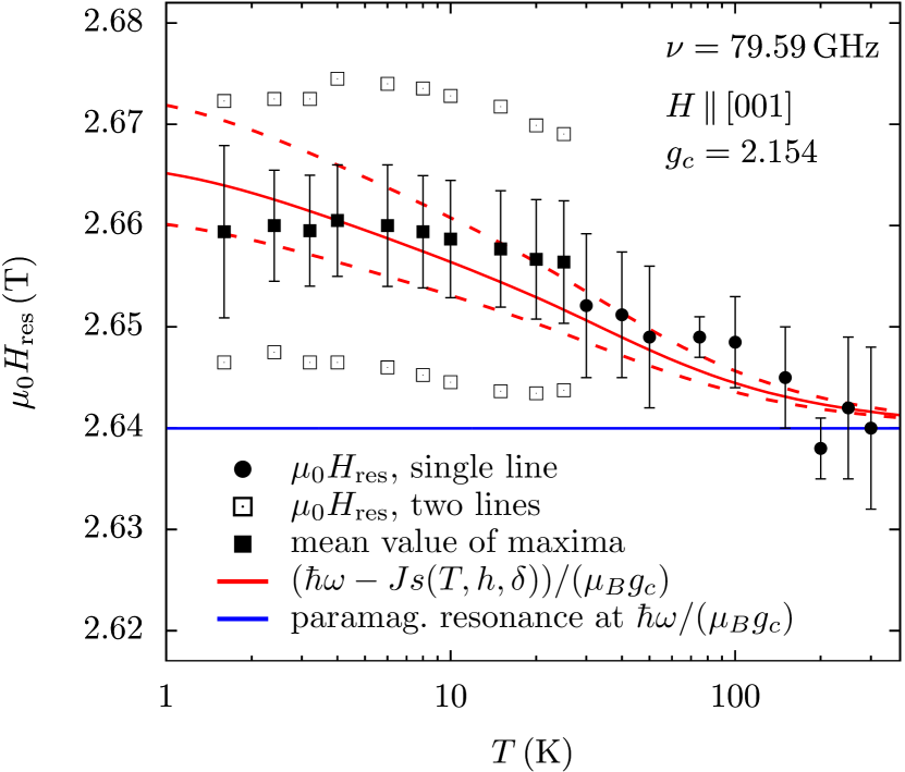
Figure 8: Resonance position for CPB as a function of temperature at $79.59\,\text{GHz}$ with the external magnetic field applied along the $c$ axis, compared with theoretical curves based on Eq. (28). The red solid line corresponds to $\delta=-0.015$, the dashed lines to $\delta=-0.012$ and $\delta=-0.019$.

The linewidth as a function of temperature, as obtained in low-frequency ESR, is shown in Fig. 9. Coming from high temperatures it increases until it reaches a maximum of $74\,\text{mT}$ at around $150\,\text{K}$ and then decreases rapidly with decreasing temperature. Below $10\,\text{K}$ this decrease is less steep and the linewidth reaches an apparently constant value of $2.5\,\text{mT}$ at $4\,\text{K}$. The behavior of the linewidth in our high-frequency experiment is very similar for high and intermediate temperatures and is also shown in Fig. 9.

For the temperature dependence of the linewidth we have no reliable theoretical prediction so far. This is due to the parameter values that characterize our compound, specifically due to the very small value of the parameter $\delta$ which causes narrow lines and would require a frequency resolution beyond the current possibilities of our numerical method (see Ref. Brockmann et al., 2012). Analytical results for the full moments, on the other hand, are available but can be only applied if the magnetic field is directed along the anisotropy axis, which is impossible as we are dealing with two inequivalent chains with anisotropy axes almost perpendicular to each other (see Sec. V.1). Moreover, these results do not compare well with the width at half height as we have explained in Sec. II and in App. B.

In the framework of the phenomenological spin diffusion theory the dynamics of the spin system is described by a diffusion equation. For a one-dimensional system the linewidth is then expected to be proportional to $T\chi(T)$ due to dominating $\bm{q}=0$ fluctuations.Ajiro et al. (1975) The product $T\chi(T)$ is also shown in Fig. 9. We fitted the curves to the data in the intermediate temperature range by adapting the constant $C$ in $CT\chi(T)$. For $T\leq 150\,\text{K}$ the linewidth follows the $T\chi(T)$ behavior but considerably deviates from it for temperatures above $150\,\text{K}$. These findings hold for the low- as well as for the high-frequency measurements. For the interpretation we should recall that spin diffusion theory is a classical phenomenology which is expected to give its best results in the high-temperature regime.

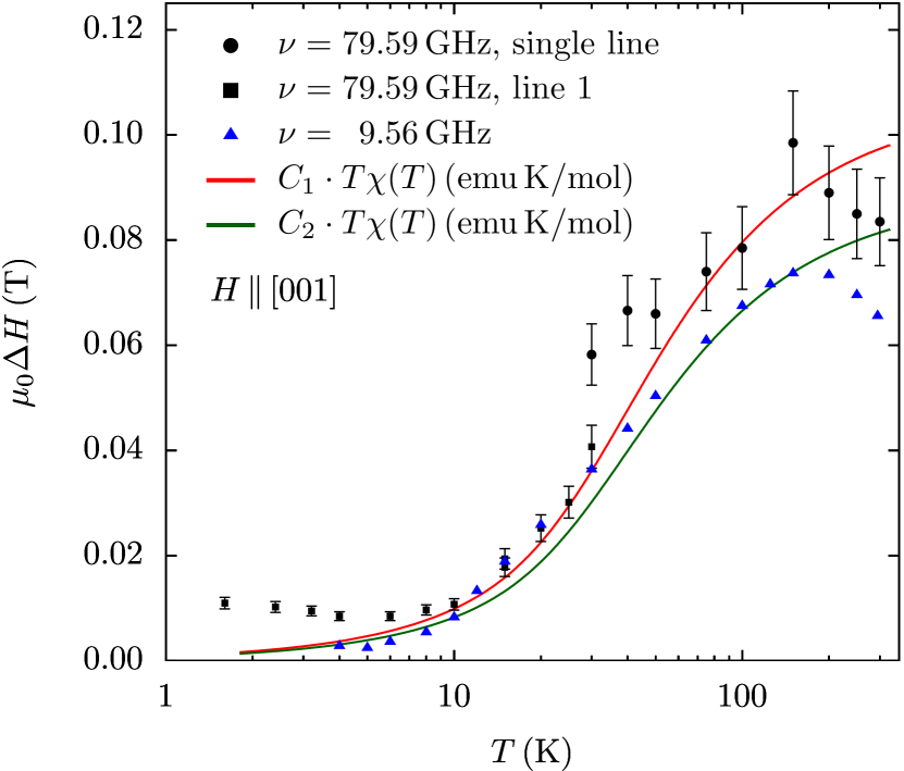
Figure 9: Linewidth for CPB as a function of temperature at $9.56\,\text{GHz}$ and $79.59\,\text{GHz}$ with the field applied along the $c$ axis. For comparison, the curves $C_{1,2}T\chi(T)$ with the static susceptibility $\chi$ of the isotropic Heisenberg chain and with $C_{1}=0.25\,\text{T\,mol/(emu\,K)}$, $C_{2}=0.2\,\text{T\,mol/(emu\,K)}$ are shown.

VI Neutron scattering

At $T_{N}\simeq 0.72$ K the magnetic moments that are assigned to the electron spins of the Cu²⁺ ions in CPB order three-dimensionally. The low-temperature neutron diffraction experiment, after refining the lattice parameters of CPB to be approximately $a=8.33$ Å, $b=17.51$ Å, $c=3.93$ Å, and $\beta=96.6^{\circ}$ at $T=1\,\text{K}$, allowed us to establish the propagation vector of the magnetic structure $\mathbf{Q}=(0,~{}0.5,~{}0.5)$, which implies a collinear ordering. Some corresponding magnetic Bragg peaks are shown in Fig. 10. They disappear around the same $T_{N}$ as the $\mu$SR and specific heat measurements suggest.Thede et al. (2012)

The observed propagation vector is fully consistent with the dominance of antiferromagnetic intrachain interaction, $J>0$. Magnetic moments of nearest neighbors in $c$ direction prefer to align in an opposite fashion. The body-centered arrangement of spins within the unit cell leads to a perfect frustration between the two chain subtypes. Probably, it could be resolved via taking the quantum fluctuations into account. Such order-by-disorder type of mechanism is known to select the most collinear arrangement from the degenerate manifold of states.Sizanov and Syromyatnikov (2011) A similar example of system with interpenetrating collinear magnetic sublattices and perfect frustration between them is found in the $S=1$ quantum magnet DTN.Sizanov and Syromyatnikov (2011); Tsyrulin et al. (2013) We thus propose a fully collinear arrangement of spins in CPB. The tentative structure is shown in Fig. 1.

This low-temperature spin structure is supported by our analysis of ESR data. Due to negativity of $\delta$ the spins prefer to align inside the plane perpendicular to the anisotropy axis (see Sec. V.1) which is for each chain the plane defined by the bromine ions (see Fig. 1). For two of the inequivalent chains these planes are almost perpendicular to each other. This leaves the antiferromagnetic arrangement of the spins along the chain as the only plausible choice for the structure (see App. C).

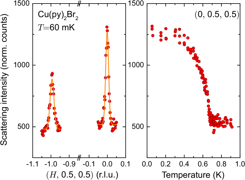
Figure 10: The results of neutron diffraction measurements on D23 instrument. Left: Neutron diffraction intensity along the ($H$, 0.5, 0.5) direction of the reciprocal space at the base temperature. Magnetic Bragg peaks of (0, 0.5, 0.5)-type are well pronounced. The solid lines are guide to the eye. Right: Diffraction intensity as function of temperature for (0, 0.5, 0.5) magnetic Bragg peak. Onset of magnetic scattering is visible around $T_{N}\simeq 0.72$ K.

VII Cu(py)₂(Cl_1-xBr_x)₂: Impact of doping

Samples with two different Cl concentrations of $2\%$ ($x=0.98$) and $5\%$ ($x=0.95$) were investigated in order to study the influence of doping at the halogen sites on spin dynamics. For both systems the angular dependence of the ESR parameters at room temperature as well as their temperature dependence was measured at $9.56\,\text{GHz}$. The former measurements are qualitatively similar to the results obtained for CPB and are not discussed any further. As in the case of the pure compound, the angular dependence could be used to identify the crystallographic $c$ axis. Measurements of the temperature dependence were performed with magnetic field applied along the $c$ axis in the range between $4\,\text{K}$ and room temperature. A small shift of the resonance fields to higher values with decreasing temperature was observed, similar to CPB.

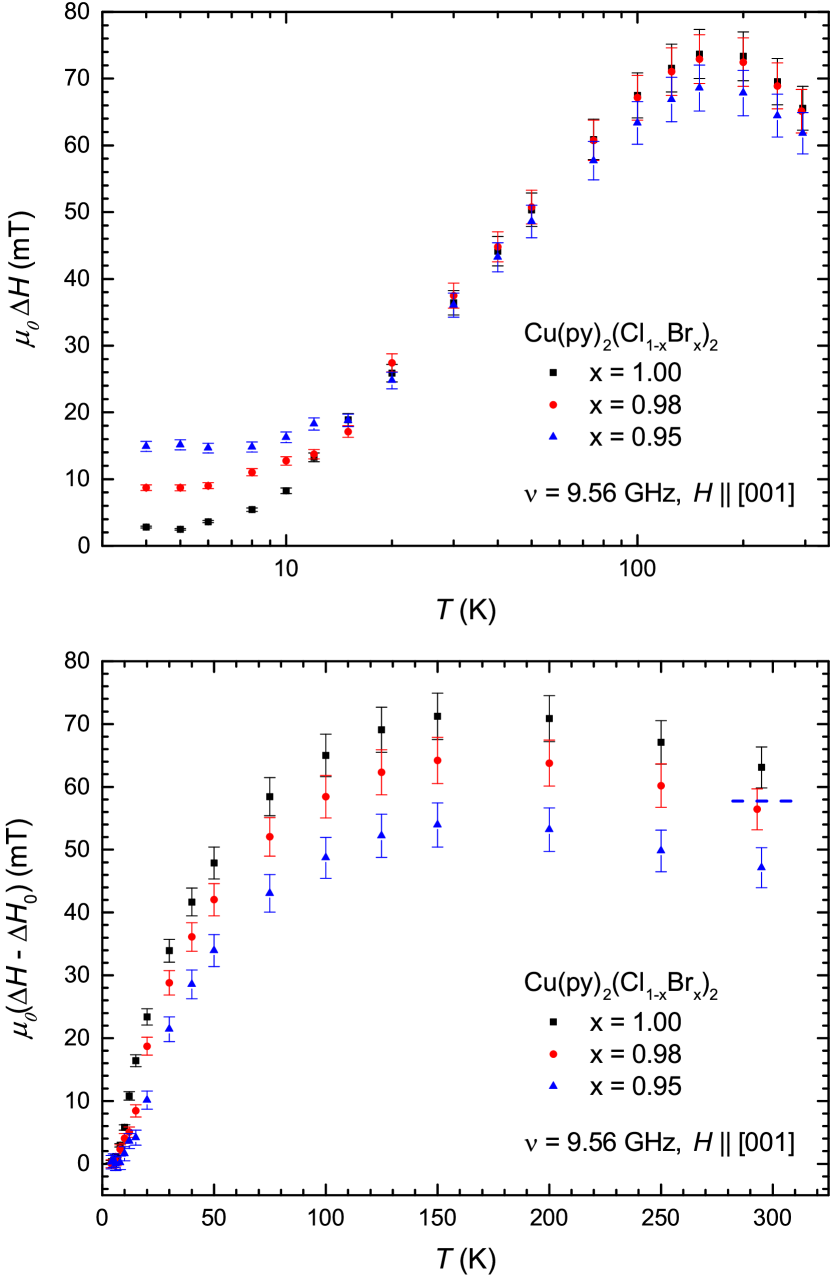
Figure 11: Temperature dependence of the ESR linewidth measured at $9.56\,\text{GHz}$ for $x=1.0,0.98,0.95$ (top) and of the contribution governed by spin dynamics obtained after subtracting the contribution of the inhomogeneous broadening (bottom). Note the difference in scales used in the upper and lower panels. The magnetic field was applied along the $c$ axis. The blue dashed line indicates the linewidth for $x=0.95$ as expected from a relative change in $J$ only.

The linewidth as a function of temperature is shown in the upper panel of Fig. 11 for all three systems studied in this work. Qualitatively, the behavior of the linewidth is the same for the three compounds. However, a constant low-temperature linewidth increases with increasing Cl concentration while at high temperatures this trend is reversed, i.e. the undoped compound shows the largest linewidth. A possible reason for this behavior lies in the different contributions to the linewidth.

The disorder in the crystals increases with increasing Cl content. Thus, the inhomogeneous broadening of the resonance lines, most likely caused by the local and spatially varying alteration of the $g$-tensor, increases with doping concentration as well. This effect is temperature independent and dominates the linewidth at low temperatures, thereby explaining the observed changes of the low-temperature linewidth.

The second contribution is given by spin dynamics of the system whose temperature dependence can be studied by subtracting the contribution of inhomogeneous broadening $\Delta H_{0}$ from the data. In the lower panel of Fig. 11 linewidths are shown after subtraction. Note the use of a linear temperature scale in this graph which is better suited for the following discussion. In the high-temperature regime, Eq. (12) holds and describes a linear relation between linewidth and isotropic exchange. In Ref. Thede et al., 2012 the strength of effective isotropic exchange was determined for CPB, CPC and various mixed compounds with different Cl and Br contents. It was found that isotropic exchange monotonically decreases with increasing Cl doping and is minimal for CPC. This is in qualitative agreement with the observed decrease of linewidth for increasing Cl content. Quantitatively, however, the relative change in $\Delta H$ is larger than the relative change in $J$. This is illustrated by a dashed horizontal line in the lower part of Fig. 11 which indicates the linewidth of the $5\,\%$ doped sample at $300\,\text{K}$ as expected from the change in $J$. Thus, the behavior of the linewidth cannot solely be described in terms of change in isotropic exchange.

A possible explanation of this finding could be an effective decoupling of anisotropic exchange from isotropic exchange, meaning that in Eq. (12) $J\delta$ might vary independently of $J$ as functions of doping. The existence of such a decoupling was shown theoreticallyTornow et al. (1999) and experimentallyKataev et al. (2001) in the case of chains with ferromagnetic exchange coupling. Note that the Cu-Br-Cu bond angle of the superexchange path is $89.64^{\circ}$, i.e. close to $90^{\circ}$ for which one would expect a ferromagnetic exchange.Goodenough (1955); Kanamori (1959); Anderson (1963) The small deviation from $90^{\circ}$ leads to an antiferromagnetic but relatively weak isotropic exchange in accordance with the experimentally determined value.

VIII Discussion

In previous sections we presented a combined experimental and theoretical study of the magnetic properties of the spin chain compounds Cu(py)₂(Cl_1-xBr_x)₂ ($x$ = 1.0, 0.98, 0.95). We begin the discussion of the obtained results by considering ESR measurements of CPB performed at low frequencies and room temperature. From studies of the angular dependence of resonance position and linewidth we inferred the existence of two distinct anisotropy axes in this system. These axes are related to the two magnetically inequivalent chain types and are oriented almost perpendicular to each other within the plane perpendicular to the chain axis. Moreover, they coincide with the axis formed by the two nitrogen ligands of the respective local octahedral environment of the Cu²⁺ ions (see Fig. 2). The insight into number and orientation of anisotropy axes in this material is an important finding, as it is an essential ingredient for modeling of our data.

Combining this knowledge with novel expressions for the angular dependence of resonance field and linewidth of individual chains (Eqs. (11) and (12), respectively) we were able to describe the observed angular dependence of both ESR parameters (see Figs. 4 and 5). Thereby, we could determine the complete $g$-tensor of the pure compound CPB. The $g$-factors obtained from the fit to our measured data of the angular dependence of resonance field and linewidth, Eq. (17), agree well with the values reported in Ref. Pal et al., 1994 for measurements of the $g$-factor angular dependence in the $a$-$c$ and $b$-$c$ planes. In Ref. Pal et al., 1994 Pal et al. found for the $g$-factor in $b$ direction $g_{b}=2.065$ which coincides with our value. The minimal and maximal values of the (effective) $g$-factor when rotating the field in the $a$-$c$ plane were found to be $g_{\text{ac}}^{\rm(max)}=2.178$ and $g_{\text{ac}}^{\rm(min)}=2.056$ around angles of $-20^{\circ}$ and $70^{\circ}$, respectively (labeled by $g_{1}$, $g_{2}$, and $\Psi$ in Tab. 1 of Ref. Pal et al., 1994). By means of our fully determined $g$-tensor we obtain $g_{\text{ac}}^{\rm(max)}=2.175$ and $g_{\text{ac}}^{\rm(min)}=2.047$ around $-25^{\circ}$ and $+65^{\circ}$. The differences in $g$-factors might be attributed to two facts. First, the authors of Ref. Pal et al., 1994 do not take into account the resonance shift due to the anisotropic exchange of the many-body system. Secondly, they assume a $g$-tensor of cylindric symmetry (only $g_{\|}$ and $g_{\perp}$ in Ref. Pal et al., 1994) whereas we consider it to be more general with three different eigenvalues $g_{1}$, $g_{2}$, and $g_{3}$. On the other hand, we assume the principal axes of the $g$-tensor to coincide with the symmetry axes of the local octahedral environment of the Cu ions, whereas in Ref. Pal et al., 1994 the angle of the maximum position of $g_{\text{ac}}$ is fitted and disagrees by about $5^{\circ}$ from our angle. Considering the width of the observed resonance lines, their data of ‘peak-to-peak’ linewidths (see Fig. 4 in Ref. Pal et al., 1994) agree well with our data for widths at half height shown in Fig. 5. The difference is a factor of about $\sqrt{3}$ which is typical for Lorentzian-like lineshapes. Thus, our results are fully consistent with previously published studies.

Furthermore, by fitting the angular dependence of the linewidth, we could derive the exponent $\gamma\approx 0.7$ of the algebraic long-time decay of a certain correlation function of the isotropic model at room temperature ($T\approx 6J/k_{B}$). This correlation function describes the propagation of two neighboring spin flips through the isotropic chain and enters our theory through the perturbation expansion in the anisotropy parameter $\delta$. It is worthwhile mentioning, that an analysis based on Eq. (12) is by no means restricted to the specific system which is discussed here. Thus, our findings may serve for the investigation of other close-to-isotropic 1d systems thereby giving insight into their spin dynamics. Finally, the fits to our angular dependent data yielded a range of reasonable values for the anisotropy parameter, $-0.04\leq\delta\leq-0.01$.

This information on $\delta$ was confirmed, and even more specified, by a detailed analysis of magnetization measurements which were performed on a CPB crystal for external fields applied parallel and perpendicular to the spin chains. The model used for the analysis takes into account the anisotropy $\delta$ of the system as well as the specific orientation of the two anisotropy axes. Therefore, it extends the existing descriptions of isotropic 1d chains like, for instance, the one employed in the approach of Ref. Johnston et al., 2000. Compared to values reported in literature, we obtained a refined value of the intrachain coupling strength $J=4.48\,\text{meV}$, i.e. $J/k_{B}=52.0\,\text{K}$, as well as the anisotropic exchange coupling $J\delta\approx-0.09\,\text{meV}$, i.e. $\delta\approx-0.02$, which was unknown up to now. The value of $J$ is close to the previously reported valueThede et al. (2012) of $J\approx 4.58\,\text{meV}$. In any case, it improves estimates obtained in Refs. Van Ooijen and Reedijk, 1977 and Jeter and Hatfield, 1972, where the authors found $J/(2\pi\hbar c)=33.2\,\text{cm}^{-1}$ and $J/(2\pi\hbar c)=37.8\,\text{cm}^{-1}$, respectively, i.e. $J/k_{B}=48\,\text{K}$ and $J/k_{B}=54\,\text{K}$, both with errors of the order of $5\%$.

We emphasize that our procedure of estimating the anisotropy from two susceptibility measurements with different field directions is not limited to the special compound CPB. The method works for any close-to-isotropic model with a small anisotropic perturbation $V$ for which the thermal expectation value of the perturbation term can be computed. This is explained in detail in App. A.1. In App. A.2 we also present a simplified method to estimate the anisotropy as well as the isotropic intrachain coupling strength which is only based on the ratio of the temperatures at the maxima of the two susceptibility curves. In the case of an isotropic system the well-known exact result of Ref. Johnston et al., 2000 is reproduced by the novel procedure. Applying the latter to our data measured on CPB, we obtained $\delta\approx-0.03$ and $J/k_{B}\approx 52.2\,\text{K}$, which is in a good agreement with values resulting from fitting magnetization data over almost the whole experimentally available temperature range. Thus, we provided expressions which might prove to be useful for an easy estimation of $J$ and $\delta$ in related systems with anisotropies being not too large.

Besides measurements of magnetization and ESR properties at low frequencies we performed a HF-ESR study on CPB in order to investigate the behavior of the resonance shift as a function of magnetic field and temperature in more detail. At high temperatures, recorded spectra consist of a single resonance line. From frequency dependent measurements at $300\,\text{K}$ we extracted the temperature-independent $g_{c}$-factor, $g_{c}=2.153$ (see Sec. V.2.1), which is very close to the X-band result $g_{c}=2.154$ and which is typical for Cu²⁺ ions in an octahedral environment.Abragam and Bleaney (2012) Afterwards, this value for $g_{c}$ was used for calculating the resonance shift at low temperatures, as it is discussed below. Moreover, we aimed at extracting an additional independent value of the anisotropy parameter from these data. As it turned out, the method of determining the anisotropy parameter $\delta$ from data for the resonance position at high temperature as a function of frequency is not reliable in the case of CPB since its anisotropy is too small ($|\delta|\approx 0.02$). However, since the quantity from which $\delta$ is estimated is proportional to $\delta^{2}$, we believe that it provides better estimates if $|\delta|$ is bigger, e.g. $|\delta|\gtrsim 0.1$. Therefore, the presented analysis may find further applications to systems beyond the scope of this work.

In contrast to high temperatures, low temperature HF-ESR spectra of the undoped sample contain two lines visible at high frequencies. For the explanation of the appearance of these two spectral lines we favor a scenario based on the existence of a (small) intergrown crystal with slightly different orientation of its $c$ axis. This would explain the different spectral weights of the two peaks (with the intensity of the smaller peak proportional to the volume of the intergrown crystal) as well as the different positions of the peaks (corresponding to different $g$-factors due to different angles between magnetic field and the two $c$ axes). This scenario is further supported by the fact that we could not observe any double-peak structure in our HF-ESR measurements on the doped samples (data not shown) which in most other respects behave qualitatively similar to the undoped sample (see Sec. VII). Another possible scenario, which cannot be fully ruled out, is that the two lines can be attributed to the two magnetically inequivalent chains. However, within this scenario we also would expect two lines of equal intensity which is in contrast to the experimental findings, rendering this scenario less likely. As it is not possible to determine the origin of the two lines definitely, we took into consideration the resonance positions of both lines as well as the mean resonance field for our investigation of the low temperature resonance shifts.

The deviations from a straight line as found in our HF-ESR measurements at $4\,\text{K}$ (see Fig. 7) could be explained by a low-temperature formula for the resonance shift, yielding a negative value of the anisotropy as well as an estimate of its magnitude $\delta=-0.012$. Furthermore, by comparing formulae stemming from different approaches we could show that the field theoretical result (26) is insufficient to explain our data for frequencies $\hbar\omega/J\gtrsim 0.1$. This evidences the importance of logarithmic corrections as in Eq. (27) for describing the resonance shift in magnetic fields which do not fulfill the condition $h/J\ll 1$ as it is the case in our study. An even better agreement between experimentally obtained and calculated shifts was found, if we take into account finite temperature effects, cf. Eq. (28), which are visible in our data despite the fact that measurements were performed for $T=0.08J/k_{B}$.

Our temperature-dependent ESR data for the resonance shift (see Fig. 8) agree very well with the theoretical prediction (28), using the previously obtained values $J/k_{B}=52.0\,\text{K}$, $g_{c}=2.154$, and $\delta\approx-0.02$ without any fitting. However, it seems that the data at very low temperatures ($T\leq 4\,\text{K}$) are better matched by assuming small anisotropies, e.g. $|\delta|=0.012$, $0.015$, instead of $|\delta|\approx 0.02$. On the other hand, the overall temperature dependence, in particular at low and intermediate temperatures, $0.1\leq k_{B}T/J\leq 3$, can be well explained by assuming a larger anisotropy, e.g. $|\delta|=0.019$ (as obtained from our susceptibility measurements). This fits with the fact that our derivation of Eq. (28) in App. B assures its validity if the the condition $\delta\ll k_{B}T/J$ is satisfied, while the extension to lower temperatures is based on more hand-waving arguments.

Furthermore, by combining the information on $\delta$ as well as on the existence of two distinct anisotropy axes with the information about the propagation vector of the ordered state, as obtained from neutron scattering experiments, a tentative spin structure at zero temperature could be proposed (see Fig. 1). Strong theoretical support for this structure was obtained from a renormalization group argument (see App. C). Thus, the present study is an example for combining ESR measurements, neutron scattering experiments, and theoretical arguments as complementary methods to gain information about the spin structure of the ordered state of a real physical system.

Considering the anisotropy parameter, we obtained at least three reliable and independent estimates for $\delta$ based on magnetization and ESR measurements which allowed us to establish the strength and the sign of the anisotropy of CPB to be $\delta\approx-0.02$. The latter finding is an important contribution to the evaluation of the utility of CPB as a realization of the XXZ model. As was mentioned in Sec. II, the XXZ model belongs to the class of integrable lattice models. This fact makes it possible to calculate its thermodynamic properties and some of its correlation functions exactly for the infinite chain. Unfortunately, an external magnetic field generally breaks the integrability, unless it is applied in the direction of the anisotropy axis. Our finding that the anisotropy axes of the two inequivalent chains in CPB are oriented perpendicular to each other and perpendicular to the chain axes makes it impossible to apply any of the known exact results for the XXZ model, except when the external field is switched off, as any finite field will necessarily be non-parallel to at least the anisotropy axis of one of the two families of inequivalent chains. For the applicability of the results obtained in Ref. Brockmann et al., 2011, for instance, we would have needed that the anisotropy axes would be oriented along the chain direction. What may be seen as bad luck with the orientation of the anisotropy axes was somewhat compensated by our finding that the anisotropy parameter is very small in modulus. This fact allowed us to perform a first order perturbation theory in $\delta$ and to use exact results for the isotropic Heisenberg chain which remains integrable for arbitrary direction of the applied magnetic field. As the comparison with the experimental results shows, this works very well for the susceptibility of the XXZ chain and for the description of the temperature dependence of the resonance shift. We have further combined the perturbative expansion in $\delta$ with a high-temperature analysis and with an analysis of the cut-off dependence of modified moments which gave us access to the angular dependence of the linewidth in the high-temperature regime. Altogether the challenges provided by the experimental data have inspired the development of new ideas on the theory side whose applicability is not restricted to our specific example but can also be applied to take into account, for instance, small XYZ anisotropy, small next-to-nearest neighbor coupling, or the coupling of adjacent chains.

In order to verify the predictionBrockmann et al. (2011) of a strong deviation from the linear dependence of the ESR resonance shift on the magnetic field in XXZ magnets, not only a material with a single anisotropy axis would be required, but we would need a material with smaller $J$ and larger $\delta$. In such a material we would also have a chance to reliably calculate cut-off dependent moments numerically which would give us direct access to the experimentally measured linewidth at half height.

IX Conclusions

A detailed theoretical analysis of the experimental data presented in this paper has shown that the magnetic properties of CPB as seen in ESR and magnetization measurements can be well understood within the following simple picture tightly connected with the crystal structure of this compound. The copper ions in the crystal form antiferromagnetic spin-1/2 chains with an exchange coupling of $J=4.48\,\text{meV}$. The local environment of a magnetic ion consists of four bromine and two nitrogen ligands which form a stretched octahedron. As a consequence of the asymmetry of this local environment, the three eigenvalues of the $g$-tensor, whose principal axes coincide with the symmetry axes of the stretched octahedron, are mutually different, $(g_{1},g_{2},g_{3})=(2.065,\,2.018,\,2.203)$.

Furthermore, the isotropic exchange interaction is distorted by a small anisotropic component. This component is well accounted for by a small Ising interaction of strength $J\delta=-0.09\,\text{meV}$ directed perpendicular to the bromine planes. As there are two types of octahedra in the material, which map onto each other by a glide reflection, there are two inequivalent spin chains whose anisotropy axes are (almost) perpendicular to each other and perpendicular to the chain direction. As compared to the intrachain coupling $J$, the interchain interaction is weak as can be seen from the small value of the ordering temperature $T_{N}=0.72\,\text{K}$, confirmed by neutron scattering experiments. Applying renormalization group arguments to the model of two weakly coupled XXZ chains (see App. C) we suggested a magnetic structure in the ordered phase ($T<T_{N}$) that is consistent with the propagation vector $\mathbf{Q}=(0,\,0.5,\,0.5)$ obtained from neutron scattering experiments and consists of antiferromagnetically ordered collinear spins oriented along the chain direction. From the dependence of the linewidth on doping concentration we found evidence for an effective decoupling of the anisotropic component $J\delta$ from the isotropic exchange $J$ as function of doping. Here the details remained open. Their explanation would require further theoretical studies.

On the theoretical side of this work, we have developed an approach to estimate the exchange anisotropy $\delta$ from static magnetization measurements with fields applied in different directions (see App. A), which is applicable to spin chain compounds with small anisotropies. Our analysis of the ESR data relied on a novel approach to computing ESR parameters from moments of the dynamical susceptibility with an inherent cut-off in frequency (see App. B). Since this approach connects the angular dependence of the linewidth with the algebraic decay in time of a certain correlation function of the isotropic Heisenberg chain, we were able to determine the corresponding exponent $\gamma$ for high temperatures experimentally.

For the future we hope from the experimental side for the development of more efficient theoretical methods for the computation of dynamical correlation functions at finite temperature which would allow us to obtain a better prediction for the behavior of the experimental linewidth at all temperatures. Our hope from the theoretical side is that the search for experimental systems with simpler geometry (such that an alignment of the magnetic field along a single anisotropy axis is possible) will be successful. At the same time, spin chain materials with bigger anisotropy and smaller $J$ (such that higher effective fields $h/J$ are accessible) are much sought after. These are expected to show an interesting non-monotonic behaviorBrockmann et al. (2011) of the resonance shift as a function of the external field.

Appendix A Static susceptibility of close-to-isotropic models

In this section we proposse a new method to obtain quantitative estimates of anisotropic perturbations of magnetically isotropic many-body systems by means of magnetization or susceptibility measurements. For simplicity we will consider magnetization and susceptibility as scalars. This is motivated by the fact that the magnetic field direction is often chosen (almost) parallel to one of the principal axes of the susceptibility tensor. The static zero-field susceptibility $\chi(T)$ can then be expressed by the magnetization $m(T,h)$ per lattice site,

$$\chi(T)=\partial_{h}m(T,h)\Big{|}_{h=0}\approx\left.\frac{m(T,h)}{h}\right|_{\text{$h$ small}}\,,$$ (29)

where the Zeeman energy $h=g\mu_{B}\mu_{0}H$ is proportional to the strength $H$ of the magnetic field. Note that the first relation in (29) implies that $J\chi(T)$ is dimensionless, like the magnetization $m(T,h)$ itself. Standard units as in Eqs. (3) and (5) can be restored in the end. The second relation in (29) assumes a linear dependence of the magnetization on the applied field which is typically justified in antiferromagnets if the field is not too large. The magnetization of CPB, discussed in the main body of the text, for instance, was measured in small residual fields of about $0.1\,\text{T}$.

The main idea to be worked out below is to measure the static zero-field susceptibility $\chi(T)$ (or equivalently the magnetization for small fields) as a function of temperature for different magnetic field directions. A comparison of the susceptibility profiles then allows us to gain information about the magnetic anisotropy of the perturbation.

A.1 Perturbation expansion of the magnetization

We consider a Hamiltonian of the form

$$\mathcal{H}=\mathcal{H}_{0}+\mathcal{H}_{Z}+\lambda V$$ (30)

with Zeeman term $\mathcal{H}_{Z}=-h\bm{S}\cdot\mathbf{e}$ and $SU(2)$-symmetric Hamiltonian $\mathcal{H}_{0}$. The operator $V$ characterizes the anisotropic perturbation. We assume that both, $\mathcal{H}_{0}$ and $V$, have the same typical energy scale $J$ and that $\lambda$ is a small dimensionless number. Furthermore, $\mathbf{e}=\hat{g}\bm{H}/|\hat{g}\bm{H}|$, where $\hat{g}$ is the $g$-tensor, will denote a unit vector in field direction, $\bm{S}=\sum_{j=1}^{L}\bm{s}_{j}$ is the total spin, and $h=\mu_{B}\mu_{0}|\hat{g}\bm{H}|$ is the Zeeman energy corresponding to the magnetic field $\hat{g}\bm{H}$. Then, the component in field direction of the dimensionless magnetization per lattice site reads

$$m(T,h,\lambda) =\frac{k_{B}T}{L}\partial_{h}\ln\left[\text{Tr}\left\{e^{-\mathcal{H}/(k_{B}T)}\right\}\right]\,.$$ (31)

A perturbation expansion up to first order in $\lambda$ yields

$$m(T,h,\lambda) \simeq m(T,h,0)-\frac{\lambda}{L}\partial_{h}\langle V\rangle_{T,h,0}\,,$$ (32)

$$\Rightarrow\quad\chi(T) \simeq\chi^{(0)}(T)-\frac{\lambda}{L}\lim_{h\to 0}\partial_{h}^{2}\langle V\rangle_{T,h,0}\,,$$ (33)

where

$$\chi^{(0)}(T)=\lim_{h\to 0}\partial_{h}m(T,h,0)\,$$ (34)

is the zero-field susceptibility of the unperturbed, isotropic system. The corrections to Eqs. (32) and (33) are of order $\mathcal{O}(\lambda^{2})$ and $\mathcal{O}(\lambda^{2}J^{2}/(k_{B}T)^{2})$, the latter meaning that temperatures are restricted to the regime $T\gg\lambda J/k_{B}$. Thus, if the temperature dependence of the zero-field susceptibility of the unperturbed isotropic model is known and if the expectation values $\langle V\rangle_{T,h,0}$ of the perturbation term with respect to the unperturbed Hamiltonian $\mathcal{H}_{0}+\mathcal{H}_{Z}$ can be computed, Eq. (33) provides a useful means to determine the anisotropy parameter $\lambda$.

Naively one might try to proceed by measuring the susceptibility of the full system, i.e. the left hand side of Eq. (33), and fitting the measured data with the computed right hand side, using $\lambda$ as a fit parameter. One problem with such kind of procedure would be that offsets and proportionality factors (like geometry factors or $g$-factors) of the measured susceptibility $\chi(T)$ are usually unknown. The energy scale $J$ may be unknown as well, whereas theoretical predictions of $J\chi^{(0)}(T)$ and $J\partial_{h}^{2}\langle V\rangle_{T,h,0}$ are typically functions of $k_{B}T/J$. In the literature an estimate of $J$ is sometimes obtained by fitting the susceptibility $\chi^{(0)}(T)$ of the isotropic Hamiltonian to measured susceptibility data, neglecting effects of small anisotropies. This value cannot be used. The coupling $J$ rather has to be extracted, together with offsets, prefactors and the anisotropy parameter $\lambda$, from the same fit. But if one uses a single susceptibility curve, the fit can become unstable since the second term in Eq. (33) is small as compared to the first one.

A considerable improvement can be achieved if several susceptibility curves are recorded with magnetic fields applied in different directions, say $\mathbf{e}^{(i)}=\hat{g}\bm{H}^{(i)}/|\hat{g}\bm{H}^{(i)}|$, $i=1,2,\ldots,n$. For the theoretical analysis we rather rotate the chain and keep the direction associated to the Zeeman term $\mathcal{H}_{Z}$ fix. A rotation does not affect the isotropic, $SU(2)$-invariant part $\mathcal{H}_{0}$ of the total Hamiltonian (30), but transforms the anisotropic part $V$ into generally different operators $V^{(i)}$. Plugging those into Eq. (33) and denoting first order terms by $\chi^{(i)}_{\text{corr}}(T)=-\frac{\lambda}{L}\lim_{h\to 0}\partial_{h}^{2}\langle V^{(i)}\rangle_{T,h,0}$ this yields

$$\chi^{(i)}(T) \simeq\chi^{(0)}(T)+\chi^{(i)}_{\text{corr}}(T)\,.$$ (35)

Taking also the possibility of different offsets $\chi^{(i)}_{0}$ and geometry factors $A^{(i)}$ for different directions $\mathbf{e}^{(i)}$ into account we arrive at ($i=1,\ldots,n$)

$$\chi^{(i)}(T) =A^{(i)}\left(\chi^{(0)}(T)+\chi^{(i)}_{\text{corr}}(T)\right)+\chi_{0}^{(i)}\,,$$ (36)

which is the general form of Eqs. (6) of the main text. Unknown parameters are offsets $\chi_{0}^{(i)}$, geometry factors $A^{(i)}$, energy scale $J$ and last but not least the anisotropy parameter $\lambda$. They can be determined by a simultaneous fit of all Eqs. (36) with $i=1,\ldots,n$ to the measured data. An advantage of a combined fit (instead of two individual fits) is that it stabilizes the algorithm. The two correction terms in Eqs. (6a) and (6b) are in a way counteractive to each other.

If one is merely interested in a rough estimate of $\lambda$ rather than in all parameters including offsets and geometry factors of the experimental susceptibility data, and if the isotropic susceptibility $\chi^{(0)}(T)$ has a maximum at a known temperature $T_{\text{max}}^{(0)}$, one can use a simplified procedure which requires no fitting and only needs two different directions of the magnetic field, labeled $1$ and $2$ in the following. It further does not require knowledge of the full temperature dependence of the isotropic susceptibility $\chi^{(0)}(T)$. If the perturbation parameter $\lambda$ is small enough the maximum of $\chi^{(0)}(T)$ at $T_{\text{max}}^{(0)}$ gets slightly shifted by $\chi^{(1,2)}_{\text{corr}}(T)$, resulting in two new maxima at $T^{(1)}_{\text{max}}$ and $T^{(2)}_{\text{max}}$. The difference of these two temperatures can be computed as

$$T^{(1)}_{\text{max}}-T^{(2)}_{\text{max}}\approx-\left.\frac{\partial_{T}\chi^{(1)}_{\text{corr}}(T)-\partial_{T}\chi^{(2)}_{\text{corr}}(T)}{\partial_{T}^{2}\chi^{(0)}(T)}\right|_{T=T^{(0)}_{\text{max}}}\,,$$ (37)

where we used expansions of $T^{(1,2)}_{\text{max}}$ up to first order in $\lambda$ and implicit differentiation. Inserting the definitions of $\chi^{(1,2)}_{\text{corr}}(T)$ and solving for $\lambda$ yields

$$\lambda\approx A_{0}\frac{T^{(1)}_{\text{max}}-T^{(2)}_{\text{max}}}{T^{(0)}_{\text{max}}}$$ (38)

with

$$A_{0}=\left.\frac{T\partial_{T}^{2}\partial_{h}\langle S^{z}\rangle_{T,h,0}}{\partial_{T}\partial_{h}^{2}\left(\langle V^{(1)}\rangle_{T,h,0}-\langle V^{(2)}\rangle_{T,h,0}\right)}\right|_{\begin{subarray}{c}h=0\\ T=T^{(0)}_{\text{max}}\end{subarray}}\,.$$ (39)

A particular example where $A_{0}$ and $T^{(0)}_{\text{max}}$ can be explicitly calculated is presented below.

A.2 Example: Spin-1/2 XXZ chain

For a single spin-1/2 XXZ chain, Eq. (1) with anisotropy/perturbation parameter $\delta=\lambda$, one can measure the zero-field susceptibility in a magnetic field parallel to the anisotropy axis ($\chi^{(\|)}$) and perpendicular to it ($\chi^{(\perp)}$). After a suitable spin rotation, which brings the Zeeman term to the form $-hS^{z}$, the corresponding perturbations become $V^{(\|)}=J\sum_{j}s_{j}^{z}s_{j+1}^{z}$ and $V^{(\perp)}=J\sum_{j}s_{j}^{x}s_{j+1}^{x}$. Their expectation values can be computed exactly by solving non-linear integral equations which arise in the context of the quantum transfer matrix approach to the thermodynamics of integrable models (see comment between Eqs. (5) and (6) of the main text). Inserting the expectation values of $V^{(\perp)}$ and $V^{(\|)}$ into Eq. (39) we obtain

$$A_{0}=\left.\frac{T\partial_{T}^{2}\partial_{h}\langle s_{1}^{z}\rangle_{T,h,0}}{J\partial_{T}\partial_{h}^{2}\langle s_{1}^{z}s_{2}^{z}-s_{1}^{x}s_{2}^{x}\rangle_{T,h,0}}\right|_{\begin{subarray}{c}h=0\\ T=T^{(0)}_{\text{max}}\end{subarray}}\approx 2.39\,,$$ (40)

where we used $T^{(0)}_{\text{max}}\approx 0.64085J/k_{B}$.Johnston et al. (2000) Therefore,

$$\lambda\approx 2.39\,\frac{T^{(\|)}_{\text{max}}-T^{(\perp)}_{\text{max}}}{T^{(0)}_{\text{max}}}\approx 2.39\left(\frac{T^{(\|)}_{\text{max}}}{T^{(\perp)}_{\text{max}}}-1\right)\,.$$ (41)

Note that in our notation used in the analysis of the compound CPB (see main body of the text, in particular Eqs. (3) and (5) in Sec. IV) the labels $(\|)$ and $(\perp)$ mean parallel and perpendicular to the crystallographic $c$ axis rather than to the anisotropy axis. Due to the special arrangement of the anisotropy axes in CPB, the difference of the two perturbation terms is minus one half of the difference of the two perturbation terms of the single anisotropic chain. Hence, the prefactor $A_{0}$ is twice as big and negative, $A_{0}\approx-4.78$, and the formula to estimate $\delta$ from the positions of the maxima reads

$$\delta\approx-4.78\left(\frac{T^{(\|)}_{\text{max}}}{T^{(\perp)}_{\text{max}}}-1\right)\,.$$ (42)

A simple fit of our CPB data around the locations of the maxima, $T\in[25\,\text{K},42\,\text{K}]$, yields $T^{(\|)}_{\text{max}}\approx 33.25\,\text{K}$, $T^{(\perp)}_{\text{max}}\approx 33.05\,\text{K}$, $T^{(\|)}_{\text{max}}/T^{(\perp)}_{\text{max}}\approx 1.006$ and hence $\delta\approx-0.03$. Note that “around the locations of the maxima” is ambiguous and that outliers and asymmetry of the maxima caused some difficulties. We determined an optimal temperature range using a polynomial of degree three as fit function.

The value of the isotropic exchange interaction can as well be estimated from the temperature value at the maximum $T^{(\|)}_{\text{max}}$ using the theoretical prediction $J/k_{B}\approx T^{(\|)}_{\text{max}}/(0.64085+\delta/8+\delta^{2}/20)\approx 52.2\,\text{K}$. The $\delta$-corrections in the denominator are obtained by varying $\delta$, calculating for each $\delta$ the quantity $k_{B}T^{(\|)}_{\text{max}}/J$ exactly, i.e. to high numerical precision by solving non-linear integral equations,Klümper (1992); Johnston et al. (2000) and approximating the resulting curve around $\delta=0$ by a polynomial of degree two. For $\delta=0$ the exact result of Ref. Johnston et al., 2000 is reproduced.

The values of $J$ and $\delta$ obtained by this simplified procedure are compatible with the values $\delta=-0.019$ and $J/k_{B}=52.0\,\text{K}$ obtained by a fit to the data over almost the entire temperature range (see Sec. IV), omitting only very low temperatures, where the perturbation expansion is not valid, and temperatures above room temperature, where the susceptibility data are less precise.

Appendix B Theoretical description of ESR parameters

In this section we discuss the ESR parameters ‘resonance shift’ and ‘linewidth’ and derive some expressions used in the main body of the manuscript. We consider an interacting spin system in a homogeneous magnetic field (in $z$ direction) which couples to the total spin. If the interactions between the spins are purely isotropic, like e.g. in Eq. (1) with $\delta=0$, the Hamiltonian of the spin system commutes with the total spin, and the dynamical susceptibility $\chi^{\prime\prime}_{+-}(\omega,h)$ of Eq. (2) simplifies to $\chi^{\prime\prime}(\omega,h)=\pi m(T,h)\,\delta(\omega-h/\hbar)$, where $m(T,h)=\langle s_{1}^{z}\rangle_{T,h,0}$ is the magnetization per lattice site. This means that the absorbed intensity has a single sharp resonance peak at the paramagnetic resonance frequency $\omega=g\mu_{B}\mu_{0}H/\hbar$. The total magnetic moment of the spin system rotates about the magnetic field direction. In a weakly anisotropic system, e.g. Eq. (1) with $\delta\neq 0$, energy is transferred from the rotation to internal excitations which causes a shift and a broadening of the paramagnetic resonance peak.

We wish to identify appropriate measures for this ‘resonance shift’ and ‘linewidth’, that are both, accessible by theory and extractable from experimental data. In the introduction of this manuscript we have discussed different measures of these ESR parameters, in the first place the maximum position of the peak and its width at half height. The latter can be easily read off from measured absorption curves, but are unfortunately so far inaccessible by theory. A measure which is more convenient for a theoretical description is defined in terms of moments of the absorption profile $I(\omega,h)/I_{0}$ (‘method of moments’; see Sec. II). It requires an integration over all frequencies or fields. This, in turn, is often problematic with experimental data, since absorption profiles away from a close vicinity of the location of the maximum of the peak may be heavily distorted by systematic and statistical errors like underground, noise, and drift.

A problem with the two different kinds of measures discussed above is that they may behave quite differently as functions of temperature and magnetic field and therefore cannot be compared naively. For instance, if we consider experimental data of the width at half height as function of temperature (see Fig. 11) and theoretical predictions for the linewidth of $I(\omega,h)$ based on its moments (see e.g. Refs. Brockmann et al., 2011, 2012), they show different monotonic behavior, and we observe a clear mismatch, in particular at low temperatures. We have discussed two possible explanations of this discrepancy in the introduction: distributions with ‘heavy tails’ and different ‘directions’ used in theory (‘$\omega$-direction’, i.e. fixed magnetic field) and in experiments (‘$h$-direction’, i.e. fixed frequency).

In order to address the first problem we shall suppress the spectral weight of the frequency tails by considering the so-called shape function $8I(\omega,h)/[\omega(1-e^{-\hbar\omega/(k_{B}T)})]$ instead of the absorbed intensity. For the XXZ spin chain with anisotropy axis parallel to the magnetic field it becomes a function of the difference $\hbar\omega-h$ in the high-temperature limit.Brockmann et al. (2012) Hence, in this limit, the second problem, the inequivalence of $h$- and $\omega$-directions, is resolved as well. We also believe that $\omega$- and $h$-directions remain more or less comparable at infinite temperature even if the anisotropy axis of the XXZ spin chain is tilted away from the direction of the magnetic field. Therefore, at high temperature, using the shape function should reduce both causes for the mismatch (‘heavy tails’ and ‘different directions’) at the same time.

At lower temperatures the situation is different. Although the spectral weight of the high-frequency tails of the normalized shape function is suppressed as compared to the weight in the tails of the absorbed intensity $I(\omega,h)/I_{0}$ (by a factor $\omega(1-e^{-\hbar\omega/(k_{B}T)})$), there is still a mismatch between experimental data and the moment-based linewidth of the numerically computed shape function.Brockmann et al. (2012) Our numerical investigations have shown that the linewidth as obtained from an integration in $h$-direction has the same monotonic behavior as the width at half height (at least for temperatures $T\geq J/k_{B}$), but a quantitative discrepancy remains between experimental linewidth, measured as width at half height, and moment-based linewidths calculated by means of the shape function.

In order to resolve this discrepancy one either has to find a way to enhance the quality of the experimental data, rendering computations of moments of the absorption line possible, or one has to find other theoretical measures for the ‘resonance position’ and ‘linewidth’ that can be computed and have a known relationship to the experimentally accessible measures ‘maximum position’ and ‘width at half height’. Below we generalize the moment-based approach by introducing certain ‘cut-off functions’ which effectively restrict the range of integration in the definition of the moments to a vicinity of the maximal absorption and suppress the experimentally inaccessible high-frequency tails.

At first sight this may look like a simple remedy to the above described problems. However, on the theoretical side, a cut-off in general spoils our method to calculate the moments. Moments are relatively easy to calculate if the cut-off is sent to infinity and if we consider the dynamical susceptibility rather than the shape function. In this case, the moments can be expressed in terms of certain static short-range correlation functions.Brockmann et al. (2011, 2012) Still, as we shall point out below, moments of a shape function restricted by a cut-off can be analyzed, if we take into account the simplifications coming from a perturbation theory in small anisotropy parameter $\delta$ and from a high-temperature expansion.

After presenting the precise definition and some properties of moments in the next subsection, we will focus on two cases. In the first case we keep the angle between magnetic field and anisotropy axis constant, $\vartheta=90^{\circ}$, and exploit only the smallness of the anisotropy. The zeroth and first moment turn out to be independent of the cut-off to lowest order in $\delta$. This means that they provide a measure for the resonance shift for all temperatures that is compatible with the experimentally determined peak position. For the second moment we have to resort to a numerical calculation of certain time-dependent correlation functions. In 3d systems the decay of these functions is fast (within a time scale of order $\hbar/J$) which leads to Lorentzian-like spectra with linewidths proportional to $\delta^{2}(1+\cos^{2}\vartheta)$. In 1d systems they decay much slower (usually algebraically as $t^{-\gamma}$), leading to possibly differently shaped spectral lines with a broader but still narrow central peak.Hennessy et al. (1973) It turns out that the small cut-off in frequency, required for the narrow absorption lines we have observed in our experiments, would make it necessary to calculate these time-dependent correlation functions for long times, which is beyond the scope of our numerical method.

In the second case we consider the angular dependence of the moments in the high-temperature regime $T\gg J/k_{B}$ and for small anisotropy parameter $\delta$. Then, the two lowest moments can be calculated explicitly and determine the angular dependence of the resonance shift. The cut-off further enables the analysis of the scaling behavior of the second moment. This scaling behavior, whose analysis is supported by numerical investigations (see below), connects the second moment with the experimentally determined width at half height. This way we derive a new formula for the angular dependence of the linewidth, Eq. (65), which is consistent with the picture of ‘inhibited-exchange narrowing’Hennessy et al. (1973) in one dimension.

B.1 Moments of the shape function

In the following we set $k_{B}=\mu_{B}=\hbar=1$. We will restore the standard units at the very end by dimensionality considerations. The function

$$f_{\alpha\beta}(\omega,h)=\frac{2}{L}\int_{-\infty}^{\infty}{\rm d}t\>e^{i\omega t}\left\langle S^{\alpha}(t)S^{\beta}\right\rangle_{T,h,\delta}$$ (43)

is called the shape function (of a chain of length $L$). The difference to the dynamical susceptibility is just a multiplicative factor $(1-e^{-\omega/T})/4$. This can be seen by expressing the function $f_{\alpha\beta}$ by its Lehmann series, as shown e.g. in Appendices A.7, 8 of Ref. Brockmann et al., 2012. The index pair $(\alpha,\beta)$ takes values $(x,x)$, $(+,-)$, and so on, depending on the polarization of the incident wave. The time evolution $S^{\alpha}(t)=e^{i\mathcal{H}t}S^{\alpha}e^{-i\mathcal{H}t}$ is governed by the Zeeman term $-hS^{z}$ of a magnetic field in $z$ direction plus the Hamiltonian of the XXZ model, where, in general, the direction of the anisotropy axis is different from the magnetic field direction. The full Hamiltonian reads

$$\mathcal{H} =\mathcal{H}_{\text{xxx}}-hS^{z}+\delta\cdot\mathcal{H}^{\prime}(\vartheta,\varphi)\,,$$ (44a)

$$\mathcal{H}_{\text{xxx}} =J\sum_{j=1}^{L}(s_{j}^{x}s_{j+1}^{x}+s_{j}^{y}s_{j+1}^{y}+s_{j}^{z}s_{j+1}^{z})\,,$$ (44b)

$$\mathcal{H}^{\prime}(\vartheta,\varphi) =J\sum_{j=1}^{L}[\cos\vartheta\,s_{j}^{z}-\frac{\sin\vartheta}{2}(e^{i\varphi}s_{j}^{+}+e^{-i\varphi}s_{j}^{-})]$$

$$\times[\cos\vartheta\,s_{j+1}^{z}-\frac{\sin\vartheta}{2}(e^{i\varphi}s_{j+1}^{+}+e^{-i\varphi}s_{j+1}^{-})]\,,$$ (44c)

where $\vartheta$ and $\varphi$ are azimuth and polar angles in the reference frame $(x,y,z)$. Thermal averages in Eq. (43) are defined by $\langle A\rangle_{T,h,\delta}=\text{Tr}\{e^{-\mathcal{H}/T}A\}/\text{Tr}\{e^{-\mathcal{H}/T}\}$.

Our aim is now to define theoretical measures of the resonance shift and the linewidth of the central peak around $\omega=h$ of the absorbed intensity $I(\omega,h)$, which can be connected to experimental measures of the ESR parameters. In the case of small anisotropy $\delta$ and not too small applied frequencies $\nu=\omega/2\pi$ of the incident micro waves we may assume that the width of this peak is small compared to the resonance field close to $h=\omega$. This assumption has several important consequences.

1. First of all, it is reasonable to assume that, when investigating only the central peak (in a proper definition of ESR parameters), it does not matter whether we consider the shape function $f(\omega,h)$ as function of frequency $\omega$ for fixed field $h$ (‘$\omega$-direction’) or the other way round (‘$h$-direction’). In this section we will focus on the former set-up.

2. Secondly, additional factors like $\omega/2$ (see paragraph below Eq. (2) of the main text) and $(1-e^{-\omega/T})/4$, which connect the shape function $f_{\alpha\beta}$ with the intensity $I$, can be neglected since they are almost constant over the whole region in which $I(\omega,h)$ is non-negligible. Hence, ESR parameters of the shape function should be comparable to those of $I$ (i.e. equal up to leading order), as long as tails of $f_{\alpha\beta}$ are not taken into account in their definition.

3. A third consequence is that for a linearly polarized incident wave we can neglect all terms in the expansion $f_{xx}=\frac{1}{4}(f_{++}+f_{+-}+f_{-+}+f_{--})$ except for $f_{+-}$. The neglected terms either belong to the peak around $\omega=-h$ and are therefore small for $\omega=h$ ($f_{-+}$) or are very small for all frequencies ($f_{\pm\pm}\ll f_{\pm\mp}$).

4. Last but not least, due to the previous point, the leading orders of the ESR parameters do not depend on $\varphi$. Hence, we may choose any value of $\varphi$ in Eq. (44c), e.g. $\varphi=0$ for convenience.

In conclusion, we may focus on the peak around $\omega=h$ of the shape function $f_{+-}$. We omit the index $+-$ and denote it by

$$f(\omega)=\frac{2}{L}\int_{-\infty}^{\infty}{\rm d}t\>e^{i(\omega-h)t}\left\langle e^{iht}S^{+}(t)S^{-}\right\rangle_{T,h,\delta}\,.$$ (45)

In order to analyze the corresponding resonance shift and linewidth we define the shifted moments

$$m_{n}(\Omega)=\int_{-\infty}^{\infty}\frac{{\rm d}\omega}{2\pi}\>\mu_{\Omega}(\omega-h)(\omega-h)^{n}f(\omega)\,.$$ (46)

This definition differs from the one of Refs. Brockmann et al., 2011, 2012 in that we have inserted a cut-off function $\mu_{\Omega}$ under the integral. As discussed in the introduction of this section, this function is supposed to suppress the high-frequency tails of the shape function that are invisible in the experiments. We imagine $\mu_{\Omega}$ as a symmetric function which falls off rapidly for large arguments and depends on a cut-off $\Omega$. To keep notations simple, we drop in the following the cut-off dependence of $\mu_{\Omega}$ and $m_{n}(\Omega)$. We consider $\mu$ together with its Fourier transform $\hat{\mu}(t)=\int_{-\infty}^{\infty}\frac{{\rm d}\omega}{2\pi}\>\mu(\omega)e^{i\omega t}$. The precise form of these functions does not matter for our arguments below. Examples are

$$\mu(\omega) =\chi_{[-\Omega,\Omega]}(\omega)\,, \hat{\mu}(t) =\frac{\sin(\Omega t)}{\pi t}\,,$$ (47a)

$$\mu(\omega) =\frac{\sin(\omega/\Omega)}{\omega/\Omega}\,, \hat{\mu}(t) =\frac{\Omega}{2}\chi_{[-\frac{1}{\Omega},\frac{1}{\Omega}]}(t)\,,$$ (47b)

$$\mu(\omega) =e^{-\frac{\omega^{2}}{2\Omega^{2}}}\,, \hat{\mu}(t) =\frac{\Omega}{\sqrt{2\pi}}e^{-\frac{t^{2}\Omega^{2}}{2}}\,.$$ (47c)

Here, $\chi_{I}$ is the characteristic function of the interval $I$. In general, we require that the cut-off function depends on a cut-off $\Omega$ in such a way that $\lim_{\Omega\rightarrow\infty}\mu(\omega)=1$.

Using the Fourier transform $\hat{\mu}(t)$, the moments can be expressed as

$$m_{n}=\int_{-\infty}^{\infty}{\rm d}t\>\hat{\mu}(t)(i\partial_{t})^{n}\hat{f}(t)\,,$$ (48)

where $\hat{f}(t)=\frac{2}{L}\left\langle e^{iht}S^{\alpha}(t)S^{\beta}\right\rangle_{T,h,\delta}$ . For the lowest moments we thus obtain the following explicit expressions,

$$m_{0} =\frac{2}{L}\int_{-\infty}^{\infty}{\rm d}t\>\hat{\mu}(t)\left\langle e^{iht}S^{+}(t)S^{-}\right\rangle_{T,h,\delta}\,,$$ (49)

$$m_{1} =\frac{2\delta}{L}\int_{-\infty}^{\infty}{\rm d}t\>\hat{\mu}(t)\left\langle e^{iht}[S^{+},\mathcal{H}^{\prime}](t)S^{-}\right\rangle_{T,h,\delta}\,,$$ (50)

$$m_{2} =\frac{2\delta^{2}}{L}\int_{-\infty}^{\infty}{\rm d}t\>\hat{\mu}(t)\left\langle e^{iht}[S^{+},\mathcal{H}^{\prime}](t)[\mathcal{H}^{\prime},S^{-}]\right\rangle_{T,h,\delta}\,.$$ (51)

The shape function is real and positive. If we divide by the zeroth moment with infinite cut-off, $m_{0}^{(\infty)}=\lim_{\Omega\to\infty}m_{n}(\Omega)$, its integral over all frequencies is normalized to one. We may therefore interpret $f(\omega)/m_{0}^{(\infty)}$ as a distribution function. If this function has a single symmetric peak, then the position of its maximum agrees with the average frequency $\langle\omega\rangle$, and the first moment becomes a measure for the resonance shift,

$$s=\langle\omega-h\rangle=m_{1}^{(\infty)}/m_{0}^{(\infty)}\,.$$ (52)

Similarly, the variance

$$\Delta\omega=\sqrt{m_{2}^{(\infty)}/m_{0}^{(\infty)}-s^{2}}$$ (53)

may be considered as a measure for the width of the peak. Such an interpretation of the variance is common within the context of Heisenberg’s uncertainty relation. Still, if the distribution function is not just a Gaussian, the variance and the more intuitive width at half height may assume rather different values. For this reason we cannot directly compare the width calculated by means of Eq. (53) with linewidths as usually obtained in ESR experiments. The only remaining question is if we can determine the moments $m_{n}(\Omega)$ theoretically for small cut-off $\Omega$, which we address in the following subsections.

B.2 Small anisotropy

The expressions for the moments simplify considerably if we expand them for small $\delta$ around the isotropic point,

$$m_{0} \simeq\frac{2}{L}\left\langle S^{+}S^{-}\right\rangle_{T,h,0}+\mathcal{O}(\delta)\,,$$ (54a)

$$m_{1} \simeq\frac{2\delta}{L}\left\langle[S^{+},\mathcal{H}^{\prime}]S^{-}\right\rangle_{T,h,\delta}+\mathcal{O}(\delta^{3})$$

$$\quad+\frac{2\delta^{2}J}{iL}\int_{-\infty}^{\infty}{\rm d}t\>\hat{\mu}(t)\int_{0}^{t}{\rm d}t_{1}\>e^{iht_{1}}$$

$$\qquad\qquad\qquad\left\langle[S^{+},\mathcal{H}^{\prime}](t_{1})[\mathcal{H}^{\prime},S^{-}]\right\rangle_{T,h,0}^{(0)}\,,$$ (54b)

$$m_{2} \simeq\frac{2\delta^{2}}{L}\int_{-\infty}^{\infty}{\rm d}t\>\hat{\mu}(t)e^{iht}\left\langle[S^{+},\mathcal{H}^{\prime}](t)[\mathcal{H}^{\prime},S^{-}]\right\rangle_{T,h,0}^{(0)}$$

$$\qquad\qquad\qquad+\mathcal{O}(\delta^{3})\,.$$ (54c)

Here the superscript $(0)$ indicates that the time evolution is generated by $\mathcal{H}_{0}=\mathcal{H}_{\text{xxx}}-hS^{z}$. As in case of the anisotropic corrections to the susceptibilities our derivation guarantees the validity of the above formulae for temperatures $T\gg\delta J$.

The most striking feature of the moments $m_{0}$ and $m_{1}$ in (54a) and (54b) is that, to lowest order in $\delta$, they do not depend on the cut-off. Hence, we may assume that the cut-off is small. Since our measured resonance peaks for CPB are moreover rather symmetric, the shift of the position of the maximum should be well described by Eq. (52) for all temperatures $T\gg\delta J$. Since the resonance shift is robust against changes of the high-frequency tails that are symmetric with respect to $\omega-h$ we expect that the validity of Eq. (52) extends down to low temperature. For the second moment, on the other hand, the cut-off dependence remains. Inserting the Hamiltonian (44) into Eqs. (54), the leading orders in $\delta$ read

$$m_{0} =\frac{4\left\langle s_{1}^{z}\right\rangle_{T,h,0}}{1-e^{-h/T}}\,,$$ (55a)

$$m_{1} =(3\cos^{2}\vartheta-1)\frac{4J\delta\left\langle s_{1}^{x}s_{2}^{x}-s_{1}^{z}s_{2}^{z}\right\rangle_{T,h,0}}{1-e^{-h/T}}\,,$$ (55b)

$$m_{2} \simeq\frac{2\delta^{2}}{L}\int_{-\infty}^{\infty}{\rm d}t\>\hat{\mu}(t)e^{iht}\left\langle[[S^{+},\mathcal{H}^{\prime}](t)[\mathcal{H}^{\prime},S^{-}]]\right\rangle_{T,h,0}^{(0)}\,.$$ (55c)

For the comparison with our experimental data we have to recall that we recorded the temperature dependence of the ESR parameters for an external field along the c axis, i.e. perpendicular to the anisotropy axes of both of the inequivalent chains in our CPB sample. This situation corresponds to $\vartheta=90^{\circ}$ and $\varphi=0$ in Eq. (44c) for both chains, which equally contribute to the resonance. With this choice of the angles, Eqs. (54a)–(54c) turn into

$$m_{0} =\frac{4\left\langle s_{1}^{z}\right\rangle_{T,h,0}}{1-e^{-h/T}}\,,$$ (56a)

$$m_{1} =\frac{4J\delta\left\langle s_{1}^{z}s_{2}^{z}-s_{1}^{x}s_{2}^{x}\right\rangle_{T,h,0}}{1-e^{-h/T}}\,,$$ (56b)

$$m_{2} \simeq\frac{\delta^{2}}{8L}\int_{-\infty}^{\infty}{\rm d}t\>\hat{\mu}(t)g_{T}(t)$$ (56c)

with

$$g_{T}(t)=\\ 4\sum_{j,k=1}^{L}\left\langle[(s_{j}^{z}s_{j+1}^{+}+s_{j}^{+}s_{j+1}^{z})(t)(s_{k}^{z}s_{k+1}^{-}+s_{k}^{-}s_{k+1}^{z})]\right\rangle_{T,h,0}^{(0)}\\ +(h\leftrightarrow-h)\,.$$ (57)

We use Eq. (52) with (56a) and (56b) in Secs. V.2.2 and V.3 in order to determine the field- and temperature-dependence of the resonance shift. As for the width we computed the correlation function in Eq. (57) numerically and tried to compare the second moment obtained from the experimental data with the theoretical value predicted by Eq. (56c). It turned out that the frequency cut-off required by the experimental data is too small for our numerically available resolution.

B.3 Small anisotropy, high temperature and low frequency

Further simplifications occur at high temperature. We consider the first three moments, Eqs. (55). For temperatures $T\gg J$ we can expand thermal averages $\langle A\rangle_{T,h,\delta}$ in the small parameter $J/T$. This way we obtain entirely explicit and cut-off independent expressions for the zeroth and first moments (neglecting subleading orders in $J/T$),

$$m_{0} \simeq 1\,,$$ (58a)

$$m_{1} \simeq\frac{J\delta}{4T}\left((1-3\cos^{2}\vartheta)h+\frac{J\delta}{2}(1+\cos^{2}\vartheta)\right)\,.$$ (58b)

On the other hand, the high-temperature expression for the second moment,

$$m_{2} \simeq\frac{J^{2}\delta^{2}}{4}\int_{-\infty}^{\infty}{\rm d}t\>\hat{\mu}_{\Omega}(t)g_{\infty}(t)\left[\frac{(1-3\cos^{2}\vartheta)^{2}}{2}\right.$$

$$+\left.5\sin^{2}\vartheta\cos^{2}\vartheta\cos(ht)+\frac{\sin^{4}\vartheta}{2}\cos(2ht)\right]\,,$$ (58c)

remains cut-off dependent and contains the infinite-temperature dynamical correlation function

$$g_{\infty}(t)=\frac{4}{L}\sum_{j,k=1}^{L}\left\langle e^{i\mathcal{H}_{\text{xxx}}t}s_{j}^{+}s_{j+1}^{+}e^{-i\mathcal{H}_{\text{xxx}}t}s_{k}^{-}s_{k+1}^{-}\right\rangle_{\infty}\,,$$ (59)

where $\langle\cdot\rangle_{\infty}=\lim_{T\to\infty}\langle\cdot\rangle_{T,h,\delta}=\text{Tr}(\cdot)/2^{L}$.

We use Eqs. (58a) and (58b) together with Eq. (52) in order to analyze the angular dependence of the resonance shift in the high-temperature regime (see Eqs. (10), (11), and (23) in Secs. V.1 and V.2.1).

The angular dependence of the linewidth at high temperatures, Eq. (12) in Sec. V.1, has been inferred from the scaling behavior of the second moment that can be calculated from (58c) under certain assumptions about the size of the cut-off and the asymptotics of the function $g_{\infty}$. The scaling behavior connects the width at half height with the second moment. The argument proceeds as follows. The ESR absorption line of our experiments consists of a single peak located at around $h=\omega$ with a width at half height of $2\eta$. It is reasonable to assume that a rescaling of the width $\eta\rightarrow a\eta$, $a>0$, amounts to a rescaling of the shape function

$$f(\omega+h)\quad\rightarrow\quad\frac{1}{a}\;f\left(\frac{\omega+h}{a}\right)\,.$$ (60)

This is true, for instance, if the ESR absorption line around the location of its maximum is shaped like a Lorentzian $f(\omega)=2\eta/(\eta^{2}+(\omega-h)^{2})$.

Under this scaling transformation the second moment (46) transforms like

$$m_{2}(\Omega)\rightarrow a^{2}m_{2}(\Omega/a)\,.$$ (61)

If now $m_{2}$ is a homogeneous function of degree $\gamma$, then $m_{2}(\Omega)\rightarrow a^{2-\gamma}m_{2}(\Omega)$. It follows that the ratio $\bigl{[}m_{2}(\Omega)\bigr{]}^{\frac{1}{2-\gamma}}/\eta$ is scale invariant and thus

$$\eta\propto\bigl{[}m_{2}(\Omega)\bigr{]}^{\frac{1}{2-\gamma}}\,,$$ (62)

which relates the width at half height with the second moment.

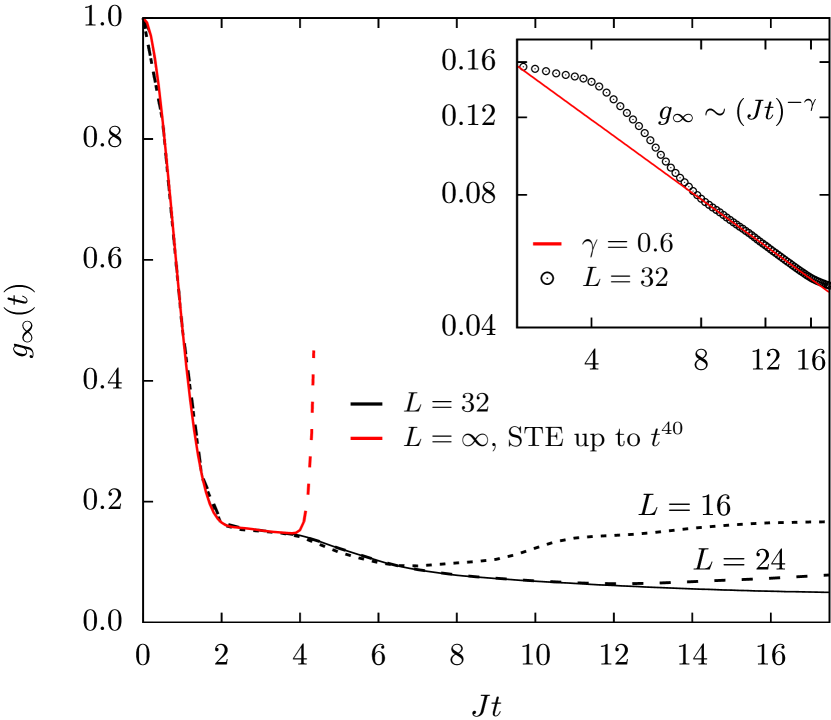
Figure 12: Dynamical correlation function $g_{\infty}$ as function of time $Jt$ for lattice sites $L=16$, $24$, and $32$ (dotted, dashed, and solid black lines) together with an exact short time expansion (STE) of the infinite chain up to $t^{40}$ (red line). Inset: data for $L=32$ in a double logarithmic plot (black circles) together with an asymptotic fit (red line) of $g_{\infty}(t)=\alpha(Jt)^{-\gamma}$ with $\gamma=0.6$ and $\alpha=0.272$.

Let us now argue that the second moment is indeed a homogeneous function of the cut-off if we restrict ourselves to an appropriate parameter regime. We hypothesize that the function $g_{\infty}$ in (59) behaves for large times, $t\gg 1/J$, as

$$g_{\infty}(t)\simeq\alpha(Jt)^{-\gamma}\,,$$ (63)

where $\alpha$ is of order one and $0<\gamma\leq 1$. We can support this claim by numerical calculations for finite system sizes up to $L=32$, as shown in Fig. 12. A fit of a straight line to the double logarithmic data in the asymptotic time regime $8\leq Jt\leq 16$ provides $\gamma=0.6$ and $\alpha=0.272$ (see inset of Fig. 12). In the main body of the text we refer to this value as $\gamma_{\infty}$, to indicate that this is the value of $\gamma$ at infinite temperature. This value is not in contradiction to the value $\gamma=0.70$ reported at the end of Sec. V.1, since this is the measured value at large but finite temperature ($T/J\approx 6<\infty$). We performed further numerical calculations at finite temperatures (down to $T/J=1$) which are in accordance with these findings.

In order to evaluate the time integral in Eq. (58c) we choose the cut-off function Eq. (47b) for our convenience. The integral in Eq. (58c) is then restricted to the interval $[-1/\Omega,1/\Omega]$. The cut-off $\Omega$ should not be too small in order to cover the whole central peak, say $\Omega\gtrsim h$. Such a choice of $\Omega$ is possible if $h\ll J$, which holds true for our measurements on CPB. We can therefore neglect all oscillations and approximate $\cos(ht)\approx\cos(2ht)\approx 1$ in Eq. (58c). We eventually obtain

$$m_{2}(\Omega)\approx\frac{J^{2}\delta^{2}(1+\cos^{2}\vartheta)}{4}\frac{2\alpha}{1-\gamma}\left(\frac{\Omega}{J}\right)^{\gamma}$$ (64)

for the cut-off dependence of the second moment.

Then, Eq. (62) implies that

$$\eta\,\propto\,J\left[\frac{\delta^{2}}{4}\left(1+\cos^{2}\vartheta\right)\right]^{\frac{1}{2-\gamma}}\,,$$ (65)

where $\delta$ is the small anisotropy parameter of the Hamiltonian (44) and $\vartheta$ the angle between magnetic field and anisotropy axis. Restoring standard units and assuming that the proportionality factor does not depend on $\vartheta$ or $\delta$, Eq. (65) turns into Eq. (12) of the main text.

Appendix C Spin configuration at zero temperature

In this section we present arguments on why the spin structure of the zero-temperature ordered ground state in CPB is as indicated by the arrows in Fig. 1, in particular why an alignment of the assigned magnetic moments along the direction of the chains is preferred. The reasoning is based on scaling arguments similar to those of Ref. Sirker et al., 2002. We interpret the interchain coupling as a small perturbation and determine the relevance of the corresponding operators in the sense of renormalization group theory. To this end, we shall calculate the large distance behavior of the correlation function of the interchain operators and compare scaling dimensions of the different terms with the marginal value of $2$, the latter being characteristic for the underlying 1+1 dimensional conformal field theory.

We consider two anisotropic spin-1/2 Heisenberg chains of type (1) with small anisotropy parameter $\delta<0$ and with anisotropy axes perpendicular to the chain direction as well as perpendicular to each other. Furthermore, the two chains are parallel and shifted against each other by half of the lattice constant (zig-zag ladder). This configuration is closely linked to the structure of the compound CPB (see the main body of the text). We assume a small isotropic (antiferromagnetic) interchain interaction, $J^{\prime}\ll J$, whose Hamiltonian reads

$$\mathcal{H}_{\rm int}=J^{\prime}\sum_{j}h_{j}\,,\quad h_{j}=\bm{s}_{j}^{(1)}\cdot\bm{s}_{j}^{(2)}+\bm{s}_{j}^{(1)}\cdot\bm{s}_{j+1}^{(2)}\,,$$ (66)

where the superscripts $(1)$ and $(2)$ distinguish the two chains. Note that for classical systems the geometrical frustration results in the vanishing of the interchain coupling for antiferromagnetically ordered chains. This is not the case for quantum chains. Still, the frustration renders the interchain coupling being a perturbation close to marginal.

Since $\delta$ is negative each single chain is in the antiferromagnetic gapless phase. We parameterize the anisotropy as $\delta=\cos\gamma-1$. For small values of $|\delta|$, the inverse relation $\gamma=\text{arccos}(1+\delta)$ can be approximated by $\gamma\approx\sqrt{2|\delta|}$. The CPB value $\delta\approx-0.02$, for instance, yields $\gamma\approx 0.2$. From conformal field theory it is known that large distance correlation functions of the XXZ Heisenberg chain at zero temperature decay asLuther and Peschel (1975); Haldane (1981)

$$\langle s_{1}^{\alpha}s_{r+1}^{\alpha}\rangle\;\sim\;\frac{(-1)^{r}}{r^{2x_{\pm}}}\,,\qquad\alpha=x,y,z\,.$$ (67)

The exponent is $2x_{+}=(1-\gamma/\pi)^{-1}$ if $\alpha$ coincides with the direction of the anisotropy axis, and it is $2x_{-}=1-\gamma/\pi$ if the $\alpha$ direction is perpendicular to it.Klümper et al. (1993) The quantities $x_{\pm}$ are called scaling dimensions of spin-spin correlation functions. Since $\gamma/\pi$ is small, e.g. $\gamma/\pi\approx 0.06$ for CPB, we can expand the first exponent as $2x_{+}=1+\gamma/\pi+\gamma^{2}/\pi^{2}$. Therefore, we have $x_{+}+x_{-}=1+\gamma^{2}/(2\pi^{2})$.

Let us fix the direction of the two chains to $z$ and the directions of their anisotropy axes to $x$ and $y$, respectively. After a straightforward calculation we obtain for the correlation function of the interchain operator $h_{j}$ in the ground state of decoupled chains

$$\langle h_{1}h_{r+1}\rangle =\sum_{\alpha,\beta}\langle{s_{1}^{\alpha}}^{(1)}({s_{1}^{\alpha}}^{(2)}+{s_{2}^{\alpha}}^{(2)}){s_{r+1}^{\beta}}^{\!\!\!\!\!\!(1)}({s_{r+1}^{\beta}}^{\!\!\!\!\!\!(2)}+{s_{r+2}^{\beta}}^{\!\!\!\!\!\!(2)})\rangle$$

$$=\!\!\sum_{\alpha=x,y,z}\langle s_{1}^{\alpha}s_{r+1}^{\alpha}\rangle^{(1)}\langle(s_{1}^{\alpha}+s_{2}^{\alpha})(s_{r+1}^{\alpha}+s_{r+2}^{\alpha})\rangle^{(2)}$$

$$\sim\;\frac{4(x_{+}^{2}+x_{-}^{2})+2(x_{+}+x_{-})}{r^{2(x_{+}+x_{-}+1)}}+\frac{4x_{-}^{2}+2x_{-}}{r^{2(2x_{-}+1)}}\,.$$ (68)

Here, the superscripts $(1)$ and $(2)$ again refer to spin operators acting on the first or on the second spin chain, respectively. The first term of the last line stems from the $\alpha=x,y$ contributions, where the spin direction is parallel to one of the anisotropy axes and perpendicular to the other one. The second term is the $\alpha=z$ contribution, where the spin direction is perpendicular to both anisotropy axes at the same time. We infer that the scaling dimension of the perturbation terms with spin direction $\alpha$ perpendicular to the chain is $x_{+}+x_{-}+1=2+\frac{\gamma^{2}}{2\pi^{2}}>2$, whereas it is $2x_{-}+1=2-\gamma/\pi<2$ for the perturbation with spin direction along the chain. The marginal scaling dimension is $2$. Therefore, the $s^{z}$-$s^{z}$ term (and only this one) represents a relevant perturbation of the critical system.

For just two weakly coupled chains this relevant perturbation would result in dimer order. In case of infinitely many chains (as in the compound CPB), however, we like to argue that true long-ranged antiferromagnetic order in the $s^{z}$ components of the local spins sets in, which can be interpreted as ‘collinear spins’.

References

- Lieb and Wu (1968) E. H. Lieb and F. Y. Wu, Phys. Rev. Lett. 20, 1445 (1968), erratum: ibid. 21 (1968) 192.
- Daley et al. (2004) A. J. Daley, C. Kollath, U. Schollwöck, and G. Vidal, J. Stat. Mech.: Theor. Exp. , P04005 (2004).
- Feiguin and White (2005) A. E. Feiguin and S. R. White, Phys. Rev. B 72, 220401 (2005).
- Schollwöck (2005) U. Schollwöck, Rev. Mod. Phys. 77, 259 (2005).
- Sirker and Klümper (2005) J. Sirker and A. Klümper, Phys. Rev. B 71, 241101 (2005).
- Fehske et al. (2008) H. Fehske, R. Schneider, and A. Weisse, Computational many-particle physics (Springer, Berlin, 2008).
- Weiße (2013) A. Weiße, Phys. Rev. E 87, 043305 (2013).
- Luther and Peschel (1975) A. Luther and I. Peschel, Phys. Rev. B 12, 3908 (1975).
- Haldane (1981) F. D. M. Haldane, J. Phys. C 14, 2585 (1981).
- Belavin et al. (1984) A. A. Belavin, A. M. Polyakov, and A. B. Zamolodchikov, Nucl. Phys. B 241, 333 (1984).
- Gogolin et al. (2004) A. O. Gogolin, A. A. Nersesyan, and A. M. Tsvelik, Bosonization and Strongly Correlated Systems (Cambridge Univ. Press, Cambridge, 2004).
- Smirnov (1992) F. A. Smirnov, Form Factors in Completely Integrable Models of Quantum Field Theory (World Scientific, Singapore, 1992).
- Mikeska and Kolezhuk (2004) H.-J. Mikeska and A. Kolezhuk, in Lecture Notes in Phys. 645 (Springer, Berlin, 2004) p. 1.
- Endoh et al. (1974) Y. Endoh, G. Shirane, R. J. Birgeneau, P. M. Richards, and S. L. Holt, Phys. Rev. Lett. 32, 170 (1974).
- Duffy et al. (1974) W. Duffy, J. E. Venneman, D. L. Strandburg, and P. M. Richards, Phys. Rev. B 9, 2220 (1974).
- Ajiro et al. (1975) Y. Ajiro, S.-i. Matsukawam, T. Yamada, and T. Haseda, J. Phys. Soc. Jpn. 39, 259 (1975).
- Thede et al. (2012) M. Thede, F. Xiao, C. Baines, C. Landee, E. Morenzoni, and A. Zheludev, Phys. Rev. B 86, 180407 (2012).
- Essler et al. (2005) F. H. L. Essler, H. Frahm, F. Göhmann, A. Klümper, and V. E. Korepin, The One-Dimensional Hubbard Model (Cambridge Univ. Press, Cambridge, 2005).
- Klümper (2004) A. Klümper, in Lecture Notes in Phys. 645 (Springer, Berlin, 2004) p. 349.
- Takahashi (1999) M. Takahashi, Thermodynamics of One-Dimensional Solvable Models (Cambridge Univ. Press, Cambridge, 1999).
- Göhmann et al. (2004) F. Göhmann, A. Klümper, and A. Seel, J. Phys. A 37, 7625 (2004).
- Boos et al. (2008) H. Boos, J. Damerau, F. Göhmann, A. Klümper, J. Suzuki, and A. Weiße, J. Stat. Mech.: Theor. Exp. , P08010 (2008).
- Klümper (1992) A. Klümper, Ann. Phys. 504, 540 (1992).
- Klümper (1993) A. Klümper, Z. Phys. B 91, 507 (1993).
- Kubo and Tomita (1954) R. Kubo and K. Tomita, J. Phys. Soc. Jpn. 9, 888 (1954).
- Ikeuchi et al. (2017) H. Ikeuchi, H. De Raedt, S. Bertaina, and S. Miyashita, Phys. Rev. B 95, 024402 (2017).
- Brockmann et al. (2011) M. Brockmann, F. Göhmann, M. Karbach, A. Klümper, and A. Weiße, Phys. Rev. Lett. 107, 017202 (2011).
- Brockmann et al. (2012) M. Brockmann, F. Göhmann, M. Karbach, A. Klümper, and A. Weiße, Phys. Rev. B 85, 134438 (2012).
- Oshikawa and Affleck (1999) M. Oshikawa and I. Affleck, Phys. Rev. Lett. 82, 5136 (1999).
- Oshikawa and Affleck (2002) M. Oshikawa and I. Affleck, Phys. Rev. B 65, 134410 (2002).
- Van Vleck (1948) J. Van Vleck, Phys. Rev. 74, 1168 (1948).
- Maeda et al. (2005) Y. Maeda, K. Sakai, and M. Oshikawa, Phys. Rev. Lett. 95, 037602 (2005).
- Trippe et al. (2010) C. Trippe, F. Göhmann, and A. Klümper, Eur. Phys. J. B 73, 253 (2010).
- Wiemann et al. (2015) Y. Wiemann, J. Simmendinger, C. Clauss, L. Bogani, D. Bothner, D. Koelle, R. Kleiner, M. Dressel, and M. Scheffler, Appl. Phys. Lett. 106, 193505 (2015).
- Hennessy et al. (1973) M. J. Hennessy, C. D. McElwee, and P. M. Richards, Phys. Rev. B 7, 930 (1973).
- Morosin (1975) B. Morosin, Acta Cryst. B31, 632 (1975).
- Johnston et al. (2000) D. C. Johnston, R. K. Kremer, M. Troyer, X. Wang, A. Klümper, S. L. Bud’ko, A. F. Panchula, and P. C. Canfield, Phys. Rev. B 61, 9558 (2000).
- Yasuda et al. (2005) C. Yasuda, S. Todo, K. Hukushima, F. Alet, M. Keller, M. Troyer, and H. Takayama, Phys. Rev. Lett. 94, 217201 (2005).
- Golze et al. (2006) C. Golze, A. Alfonsov, R. Klingeler, B. Büchner, V. Kataev, C. Mennerich, H.-H. Klauss, M. Goiran, J.-M. Broto, H. Rakoto, S. Demeshko, G. Leibeling, and F. Meyer, Phys. Rev. B 73, 224403 (2006).
- Bonner and Fisher (1964) J. C. Bonner and M. E. Fisher, Phys. Rev. 135, A640 (1964).
- Hieida et al. (2001) Y. Hieida, K. Okunishi, and Y. Akutsu, Phys. Rev. B 64, 224422 (2001).
- Dmitriev et al. (2002) D. V. Dmitriev, V. Y. Krivnov, A. A. Ovchinnikov, and A. Langari, Sov. Phys. JETP 95, 538 (2002).
- Pal et al. (1994) S. Pal, R. Samanta(Sikdar), and A. Pal, J. Phys. Chem. Solids 55, 1315 (1994).
- Abragam and Bleaney (2012) A. Abragam and B. Bleaney, Electron Paramagnetic Resonance of Transition Ions (Oxford Univ. Press, Oxford, 2012).
- Psaroudaki et al. (2014) C. Psaroudaki, J. Herbrych, J. Karadamoglou, P. Prelovšek, X. Zotos, and N. Papanicolaou, Phys. Rev. B 89, 224418 (2014).
- Sizanov and Syromyatnikov (2011) A. V. Sizanov and A. V. Syromyatnikov, J. Phys.: Condens. Matter 23, 146002 (2011).
- Tsyrulin et al. (2013) N. Tsyrulin, C. D. Batista, V. S. Zapf, M. Jaime, B. R. Hansen, C. Niedermayer, K. C. Rule, K. Habicht, K. Prokes, K. Kiefer, E. Ressouche, A. Paduan-Filho, and M. Kenzelmann, J. Phys.: Condens. Matter 25, 216008 (2013).
- Tornow et al. (1999) S. Tornow, O. Entin-Wohlman, and A. Aharony, Phys. Rev. B 60, 10206 (1999).
- Kataev et al. (2001) V. Kataev, K.-Y. Choi, M. Grüninger, U. Ammerahl, B. Büchner, A. Freimuth, and A. Revcolevschi, Phys. Rev. Lett. 86, 2882 (2001).
- Goodenough (1955) J. B. Goodenough, Phys. Rev. 100, 564 (1955).
- Kanamori (1959) J. Kanamori, J. Phys. Chem. Solids 10, 87 (1959).
- Anderson (1963) P. W. Anderson, Solid State Phys. 14, 99 (1963).
- Van Ooijen and Reedijk (1977) J. A. C. Van Ooijen and J. Reedijk, Inorg. Chim. Acta 25, 131 (1977).
- Jeter and Hatfield (1972) D. Y. Jeter and W. E. Hatfield, J. inorg. nucl. Chem. 34, 3055 (1972).
- Sirker et al. (2002) J. Sirker, A. Klümper, and K. Hamacher, Phys. Rev. B 65, 134409 (2002).
- Klümper et al. (1993) A. Klümper, T. Wehner, and J. Zittartz, J. Phys. A 26, 2815 (1993).