Eliminating Inertia in a Stochastic Model of a Micro-Swimmer with Constant Speed

Abstract

We are concerned with the dynamical description of the motion of a stochastic micro-swimmer with constant speed and fluctuating orientation in the long time limit by adiabatic elimination of the orientational variable. Starting with the corresponding full set of Langevin equations, we eliminate the memory in the stochastic orientation and obtain a stochastic equation for the position alone in the overdamped limit. An equivalent procedure based on the Fokker-Planck equation is presented as well.

1 Introduction

Recently, there has been an increasing interest in biology, physics and chemistry in so-called active particles niwa1994 ; vicsek1995 ; marchetti.c:2013 ; romanczuk.p:2012 ; hauser_spec . These units are equipped with some kind of propulsive mechanism which enables them to transform energy into motion, and therefore represent systems far from thermodynamic equilibrium. Active particles are extensively studied from the experimental as well as from the theoretical point of view. Examples of corresponding studies range from investigations of the dynamical behavior of individual units like motile cells schienbein.m:1993 ; teeffelen2008 ; selmeczi2008 ; bodeker2010 ; li_persistent_2008 ; Amselem ; dilao_chemotaxis_2013 ; hauser15 , over macroscopic animals bazazi2010 ; RomRom15 and artificial self-propelled particles paxton2004 ; howse2007 ; ruckner2007 ; kumar2008 ; kudrolli2008 ; tierno2010 ; ke_motion_2010 ; takagi13 , to many body interactions and collective phenomena in many-particle systems vicsek1995 ; gregoire04 ; chate2006 ; buhl_disorder_2006 ; Bertin06 ; Ihle2011 ; Ihle2013 ; grossman2013 ; grossmann2016 ; hamid16 ; patch2017 .

We will concentrate on models describing the stochastic motion of an individual active particle. Such particles are often called Active Brownian Particles (ABP) because of their similarities to normal Brownian motion romanczuk.p:2012 ; schweitzer.f:1998 ; schweitzer.f:2007 . Thus, at large time scales both exhibit diffusive behavior, as calculations of the mean square displacement confirm mikhailov . Moreover, a crossover from an initial, ballistic to the final, diffusive behavior have been reported romanczuk.p:2012 ; mikhailov ; Peruani as it is known for passive particles langevin1908 and for correlated random walks shigesada ; okubo . Differences occur since an ABP is an object out of equilibrium contrary to a normal Brownian particle whose motion corresponds to an equilibrium situation ebeling.w:1999 ; erdmann_brownian_2000 . The fluctuating forces acting on ABP originate from the active nature of the system, such as fluctuations of the propulsion, and not from thermal noiseromanczuk.p:2011 ; sevilla14 .

More precisely, we will report on a stochastic micro-swimmer moving with constant speed which is a special ABP romanczuk.p:2012 . Fluctuating forces act only perpendicular to the instantaneous direction of motion. If these can be described by white noise, the swimmer performs persistent ballistic motion at small time scales and diffusive motion at larger scales, similarly to a Brownian particle mikhailov . For a Brownian particle as well as for an ABP including the micro-swimmer under consideration, the ballistic regime is caused by the inertia of the object. Therefore, the description of these two regimes, and of the transition between them requires a formulation of the equations of motion in phase space, including coordinates and velocity components, or of the corresponding kinetic equations for joint probability densities thereof. By contrast, as well known, if only the diffusive regime is of interest, the system can be modeled by a much simpler overdamped dynamics Kramers ; Becker52 for coordinates alone, and the effects of inertia, describing the memory in the velocity variable, can be eliminated. Then, the velocity as a variable follows instantaneously and without memory the forces acting on the particle.

We will elaborate on such a procedure for the stochastic micro-swimmer with constant speed. The variable introducing inertia in this model, which has to be eliminated, is the orientation of the velocity. The latter creates the persistent ballistic motion at small time scales but does not have relevance for the diffusive regime observed at larger time scales. The consistent procedure of adiabatic elimination of this orientational variable is the main topic of the present work.

First, in $\mathrm{Sec.}$ 2, we review the adiabatic elimination of the velocity in the description of the normal Brownian particle Becker52 . It is presented for the Langevin equation as well as on the level of a kinetic approach, which is similar to the transport theory in gas dynamics Rumer80 . A similar systematic reduction procedure in case of ABPs is nowadays still missing. Here, we fill this gap for the simple case of a micro-swimmer with constant speed as studied in haeggqwist ; weber11 ; weber12 ; Thiel2012 ; noetl2017 ; mijalkov2013 ; volpe2014 ; geiseler2016 ; geiseler2016kramers ; debnath ; btenhagen ; babel and in many other applications. We will proceed in a similar way as it is presented in $\mathrm{Sec.}$ 2 for a passive Brownian particle. The corresponding new procedure is presented in $\mathrm{Sec.}$ 3 again on the level of the Langevin equation and also for the kinetic approach. In $\mathrm{Sec.}$ 4 we summarize our findings.

2 Adiabatic Elimination for Brownian particles

The theory of Brownian motion is connected with such famous names as Einstein einstein1905 , Langevin langevin1908 and Smoluchowski smoluchowski1906 . It was a great success of the developing statistical physics at the beginning of the 20${}^{\text{th}}$ century being one of the first descriptions of dynamical fluctuations using stochastic methods. Starting point of the description was the formulation of a Chapman-Kolmogorov-like relation for the probability density of the particle by Einstein. Soon later, Langevin claimed to have found an infinitely simpler approach based on a stochastic differential equation. Both, together with Smoluchowski, can thus be identified as being pioneers in the developing tools for stochastic dynamical problems.

2.1 Adiabatic elimination I: Langevin equation

Langevin’s approach started from Newtonian dynamics in the presence of friction and impacts described as noise force. Therefore, he explicitly took into account inertia leading to the persistence of the motion. Einstein, by contrast, obtained results for the overdamped regime with high damping of the fluid or small masses of the particles, where inertia can be neglected.

For the two-dimensional position vector $\mathbf{r}(t)\,=\,(x,y)$ and the velocity $\mathbf{v}(t)\,=\,(v_{x}.\,v_{y})$ of the particle, the Langevin approach corresponds to equations of motion (in the nowadays accepted notation) borkovec_1990

$$\frac{\mathrm{d}\,\mathbf{r}}{\mathrm{d}\,t}\,\,=\,\mathbf{v},\leavevmode\nobreak\ \leavevmode\nobreak\ \leavevmode\nobreak\ \leavevmode\nobreak\ \leavevmode\nobreak\ \leavevmode\nobreak\ m\,\frac{\mathrm{d}\,\mathbf{v}}{\mathrm{d}\,t}\,\,=\,-\gamma\,\mathbf{v}\,+\,\sqrt{2\gamma k_{\rm B}T}\,\boldsymbol{\xi}(t),$$ (1)

where $m$ is the mass of the particles and $k_{\rm B}T$ is the thermal energy. The two terms at the r.h.s. of the second equation describe the interaction with the surrounding liquid. The first one stands for the Stokes friction with coefficient $\gamma$ and the second one models molecular agitation wherein $\boldsymbol{\xi}=(\xi_{x},\xi_{y})$ is a Gaussian noise with vanishing mean, having independent components $\xi_{i}$ and is $\delta$-correlated in time, i.e.

$$\left\langle\boldsymbol{\xi}(t)\right\rangle\,=\,0,\leavevmode\nobreak\ \leavevmode\nobreak\ \leavevmode\nobreak\ \leavevmode\nobreak\ \leavevmode\nobreak\ \left\langle\xi_{i}(t)\,\xi_{j}(t^{\prime})\right\rangle\,=\,\delta_{i,j}\delta\,(t-t^{\prime})\,,\leavevmode\nobreak\ \leavevmode\nobreak\ \leavevmode\nobreak\ i,j\,=\,x,y.$$ (2)

The prefactor of the noise term is called the noise intensity. It was selected such that the particle’s velocity obey a Maxwellian distribution in equilibrium. The latter is established for $t\gg\tau_{\gamma}=m/\gamma$ where $\tau_{\gamma}$ is the relaxation time of the particle in the fluid. Hence, the mean squared velocity fulfills the equipartition requirement $m{v}_{i}^{2}/2=k_{B}T/2,\,(i=x,y)$. The connection of the noise intensity with the friction coefficient is a static version of the fluctuation-dissipation relation.

Integration of this system of equations yields the well known mean squared displacement (MSD). In detail, for the initial condition $\vec{r}(t=0)=\vec{r}_{0}=0$, it reads in $d$ dimensions langevin1908

$$\left\langle\mathbf{r}^{2}(t)\right\rangle\,=\,{\color[rgb]{0,0,0}2\,d}\,\frac{k_{\rm B}T}{\gamma}\,\left[t\,+\,\frac{m}{\gamma}\left(\exp(-\frac{\gamma}{m}t)-1\right)\right]\,.$$ (3)

For times $t\,\ll\,\tau_{\gamma}$ ballistic behavior is found. Oppositely, for $t\,\gg\,\tau_{\gamma}$ diffusive behavior with a linear growth of the MSD with respect to time is observed. The corresponding time domains can be translated into distances traveled: at distances smaller than $l_{\gamma}$ the behavior is ballistic, and crosses over to diffusion at distances larger $l_{\gamma}$. The crossover time is given by the relaxation time $\tau_{\gamma}$, and $l_{\gamma}$ is known as the brake path, $l_{\gamma}\,=\,\tau_{\gamma}\,\sqrt{k_{\rm B}T/m}\,$ Becker52 ; Hwalisz . In the long-time limit, $t\,\gg\,\tau_{\gamma}$, when displacements are larger than the brake path $l_{\gamma}$, this result coincide with Einstein’s finding einstein1905 and the diffusion coefficient reads approximately

$$D_{\mbox{\tiny eff}}\,=\,\,\frac{1}{2\,d\,t}\,\left\langle\mathbf{r}^{2}(t)\right\rangle\,\approx\,\frac{k_{\rm B}T}{\gamma}\,.$$ (4)

The approximation is valid by assuming either the mass being small or the friction being large. Therefore, this limit is called nowadays “overdamped”.

Being interested only in this coarse-grained long-time limit $t\gg\tau_{\gamma}$ and $|{\mathbf{r}}|\gg l_{\gamma}$, one might reduce the integration scenario by neglecting the inertia term in (1). To do this, one usually processes by collecting the large items at the r.h.s. of the differential equation, i.e. one formulates borkovec_1990 ; Hwalisz ; haken ; gardiner ; gardiner:82 ; ucna ; lsg_talkner ; sancho

$$\frac{\mathrm{d}\,{\mathbf{v}}}{\mathrm{d}\,t}\,\,=\,-\frac{1}{\tau_{\gamma}}\left(\,\mathbf{v}\,-\,\sqrt{2\frac{k_{\rm B}T}{\gamma}}\,\boldsymbol{\xi}(t)\right).$$ (5)

Since $\tau_{\gamma}$ shall be small the items on the r.h.s. are large supposed that the value of $k_{\rm B}T/\gamma$ remains finite. Then, the l.h.s. of Eq.(5) becomes negligible compared to each of the two items at the r.h.s. which therefore have to compensate each other. Thus effectively it holds that

$$\mathbf{v}\,=\,\sqrt{2\frac{k_{\rm B}T}{\gamma}}\,\boldsymbol{\xi}(t).$$ (6)

The validity is also proven since all higher moments of this expression exist. Hence, as seen in Eq. (6), for time scales larger than $\tau_{\gamma}$ and with the assumed coarse-graining, the velocity does not change smoothly but becomes irregular white noise $\mathbf{v}(t)\propto\boldsymbol{\xi}(t)$. In consequence, the autocorrelation function (ACF) of the velocity becomes $\delta$-like reading

$$K_{\mathbf{v},\mathbf{v}}(t\,-\,t^{\prime})\,=\,\left\langle\mathbf{v}(t)\cdot\mathbf{v}(t^{\prime})\right\rangle\,=\,{\color[rgb]{0,0,0}2\,d}\,\frac{k_{\rm B}T}{\gamma}\,\delta(t-t^{\prime})\,.$$ (7)

Eventually, insertion of this velocity vector into the first equation of $\mathrm{Eq.}$ (1) defines the well-known overdamped dynamics for the position of a Brownian particle borkovec_1990

$$\frac{\mathrm{d}\,\mathbf{r}}{\mathrm{d}\,t}\,\,=\,\sqrt{2\,\frac{k_{\rm B}T}{\gamma}}\,\boldsymbol{\xi}(t)\,,$$ (8)

with $\boldsymbol{\xi}(t)$ being a Gaussian white noise with properties defined in (2).

Since the noise is additive we can simply integrate this equation and obtain, after averaging over different realizations of the noise, for the MSD

$$\left\langle\mathbf{r}^{2}(t)\right\rangle\,=\,\int_{0}^{t}\int_{0}^{t}\,{\rm d}t\,{\rm d}t^{\prime}\,K_{\mathbf{v},\mathbf{v}}(t-t^{\prime}).$$ (9)

After taking the integral over the ACF $K_{\mathbf{v},\mathbf{v}}$ using (7) one finds for the effective diffusion coefficient exactly the r.h.s. of (4).

2.2 Adiabatic elimination II: Kinetic approach

Elimination of velocities is also possible when starting from the Fokker-Planck equation (FPE) for the conditional probability density function $P(\mathbf{r},\mathbf{v},t|\mathbf{r}_{0}=0,\mathbf{v}_{0},t_{0})$, which is the transition probability density to find the position and velocity in an infinitesimal element ${\rm d}\mathbf{r}{\rm d}\mathbf{v}$ around $\mathbf{r}$ and $\mathbf{v}$ of the phase space at time $t$ having started at $t_{0}=0$ at the origin and with the initial velocity $\mathbf{v}_{0}$, for simplicity. The corresponding FPE reads

$$\frac{\partial\,P}{\partial\,t}\,\,=\,-\mathbf{v}\,\cdot\,\frac{\partial\,P}{\partial\,\mathbf{r}}\,\,+\,\frac{\gamma}{m}\,\frac{\partial\,}{\partial\,\mathbf{v}}\,\cdot\left(\,\mathbf{v}\,P\,+\,\frac{k_{\rm B}T}{m}\,\frac{\partial\,P}{\partial\,\mathbf{v}}\,\right).$$ (10)

We would like to mention that already Kramers in his seminal work Kramers found an elegant way to eliminate the velocity. Using the factorizing properties of the Fokker-Planck operator, he was able to derive the diffusion equation for the marginal probability density $\rho(\mathbf{r},t)$ of the position of the Brownian particle by integrating the FPE (10) over the velocity along an inclined straight line (see also the discussion in the excellent book by Becker Becker52 ). Later, many other approaches have been formulated, including projection operator formalism haken ; gardiner ; gardiner:82 . To our best knowledge none of these approaches has been applied successfully to the problems of ABP so far. Therefore here we use a kinetic approach which is based on transport equations for the first three moments of the velocity. We first demonstrate this approach in application to a Brownian particle. Later on, the approach is successfully applied to the situation of the stochastic micro-swimmer with constant speed.

The asymptotic solution for the marginal distribution of $\mathbf{v}$ is a Gaussian corresponding to the Maxwell distribution of velocities. In correspondence to the kinetic theory of gases, the space- and time-dependent zeroth, first and second moments of the velocity are introduced. These are the marginal probability density for the position $\rho(\mathbf{r},t)$, the mean velocity with components $u_{i}(\mathbf{r},t)$, and the variances $\braket{\delta v_{i}\,\delta v_{j}}(\mathbf{r},t)$ of the deviations from the mean velocity $\delta v_{i}\,=\,v_{i}\,-\,u_{i}$. In detail, they are defined as

$$\rho(\mathbf{r},t)\,=\,\int P(\mathbf{r},\mathbf{v},t){\rm d}\mathbf{v}\,,\leavevmode\nobreak\ \leavevmode\nobreak\ \leavevmode\nobreak\ \leavevmode\nobreak\ \leavevmode\nobreak\ \leavevmode\nobreak\ \rho(\mathbf{r},t)\,u_{i}(\mathbf{r},t)\,=\,\int v_{i}P(\mathbf{r},\mathbf{v},t){\rm d}\mathbf{v}\,,$$ (11)

$$\rho(\mathbf{r},t)\,\braket{\delta v_{i}\,\delta v_{j}}(\mathbf{r},t)\,=\int(v_{i}-u_{i}(\mathbf{r},t))\,(v_{j}-u_{j}(\mathbf{r},t))\,P(\mathbf{r},\mathbf{v},t){\rm d}\mathbf{v}\,,\leavevmode\nobreak\ \leavevmode\nobreak\ \leavevmode\nobreak\ i,\,j\,=\,x,\,y.$$

In kinetics these moments obey the transport equations which are balance equations for the marginal density, momentum and temperature Rumer80 . In our notation starting from the FPE (10) and by corresponding multiplications and integrations we derive:

$$\frac{\partial\,\rho}{\partial\,t}\,+\frac{\partial\,}{\partial\,x_{k}}\,\rho\,u_{k}\,=0,\leavevmode\nobreak\ \leavevmode\nobreak\ \leavevmode\nobreak\ \leavevmode\nobreak\ \leavevmode\nobreak\ \leavevmode\nobreak\ \leavevmode\nobreak\ \leavevmode\nobreak\ \frac{\partial\,u_{i}}{\partial\,t}\,+u_{k}\frac{\partial\,u_{i}}{\partial\,x_{k}}\,=-\frac{\gamma}{m}u_{i}{\color[rgb]{0,0,0}-}\frac{1}{\rho}\frac{\partial\,\rho\braket{\delta v_{i}\,\delta v_{k}}}{\partial\,x_{k}}\,,$$ (12)

$$\frac{\partial\,\braket{\delta v_{i}\,\delta v_{j}}}{\partial\,t}\,\,+\,u_{k}\frac{\partial\,\braket{\delta v_{i}\,\delta v_{j}}}{\partial\,x_{k}}\,\,=$$ (13)

$$\leavevmode\nobreak\ \leavevmode\nobreak\ \leavevmode\nobreak\ \leavevmode\nobreak\ \leavevmode\nobreak\ \leavevmode\nobreak\ \leavevmode\nobreak\ \leavevmode\nobreak\ \leavevmode\nobreak\ \leavevmode\nobreak\ \leavevmode\nobreak\ \leavevmode\nobreak\ \leavevmode\nobreak\ \leavevmode\nobreak\ =\,2\frac{\gamma}{m}\left(\frac{k_{\rm B}T}{m}\delta_{i,j}\,-\,\braket{\delta v_{i}\,\delta v_{j}}\right)\,-\,\braket{\delta v_{i}\,\delta v_{k}}\frac{\partial\,u_{j}}{\partial\,x_{k}}\,\,-\,\braket{\delta v_{j}\,\delta v_{k}}\frac{\partial\,u_{i}}{\partial\,x_{k}}\,$$

with $i,j,k=x,y$; the summation over the repeating indices is assumed. We close the equations by neglecting third moments of deviations from the mean velocity, i.e. by assuming $\braket{\delta v_{i}\delta v_{j}\delta v_{k}}\approx 0$.

We now examine the asymptotic behavior of these quantities at times longer than the relaxation time $t\,\gg\,\tau_{\gamma}$. In this limit, the first bracket on the r.h.s. of the equation for the variances becomes dominant since $\gamma/m=\tau_{\gamma}^{-1}$ is a large parameter. Therefore, we can neglect the substantial derivative on the l.h.s. of the dynamics and the remaining items on the r.h.s. yielding in zeroth order of small $\tau_{\gamma}$

$$\ \braket{\delta v_{i}\,\delta v_{j}}(\mathbf{r},t)\,\approx\,\frac{k_{\rm B}T}{m}\,\delta_{i,j}\,+\,\mathcal{O}(\tau_{\gamma})\,.$$ (14)

The cross-correlations disappear, and the standard deviations for both directions coincide, become homogeneous, and are time-independent.

Similarly, we proceed for the mean velocity. The substantial derivative can be assumed to be small compared to the two terms on the r.h.s. of the equation for the mean velocity at large time scales. The mean velocity will follow the evolution of the slowly developing density. In consequence, after insertion of (14) the mean flux in the position space becomes

$$\rho(\mathbf{r},t)\,u_{i}(\mathbf{r},t)\,=\,\frac{m}{\gamma}\,\frac{\partial\,}{\partial\,x_{k}}\,\,\rho\,\braket{\delta v_{i}\,\delta v_{k}}\approx\,-\,\frac{k_{\rm B}T}{\gamma}\,\frac{\partial\,\rho}{\partial\,x_{i}}\,.$$ (15)

The latter is a kind of Fick’s law for the density flux $\rho(\mathbf{r},t)\,u_{i}(\mathbf{r},t)$. Thus, what remains as a result of the adiabatic elimination of the mean velocity and of the variances is the resulting continuity equation for the density which reads

$$\frac{\partial\,\rho}{\partial\,t}\,\,=\,\,\frac{k_{\rm B}T}{\gamma}\,\left(\frac{\partial^{2}}{\partial x^{2}}\,+\,\frac{\partial^{2}}{\partial y^{2}}\right)\,\rho(\mathbf{r},t).$$ (16)

Eq.(16) describes the normal diffusion of the Brownian particles, and is the equation derived by Einstein in 1905 einstein1905 . It includes the effective diffusion coefficient as defined in (4). Hence, by making effectively the same approximation as in the Langevin approach, we derived the well-know equation for the probability density $\rho(\mathbf{r},t)$ describing the diffusive behavior in the overdamped regime. Both approaches, the overdamped Langevin dynamics (8) and the diffusion equation for the probability density (16) are equivalent models for the description of the probabilistic motion of a Brownian particle. In the next section we introduce the stochastic micro-swimmer with constant speed. For the latter we will apply the same approach to formulate an effective overdamped dynamics for the individual equation of motion as well as for the kinetic equation for the probability density.

3 Stochastic Micro-swimmer

3.1 Active Brownian particle with constant speed

The new physics, making the particle to an active one, can be best formulated on the level of the Newtonian law for a self-propelled object. Here we consider the two-dimensional case of an ABP; the point particle is described by its position $\mathbf{r}(t)$ and velocity $\mathbf{v}(t)$ at time $t$. Particles have a polarity which points always along the current velocity and is represented by an unit vector $\mathbf{e}_{v}(t)$ in the direction of velocity . In polar coordinates (with the polar axis coinciding with the abscissa of the Cartesian system) we have

$$\mathbf{e}_{v}(t)\,=\,\left(\cos\phi(t),\sin\phi(t)\right),\leavevmode\nobreak\ \leavevmode\nobreak\ \leavevmode\nobreak\ \leavevmode\nobreak\ \leavevmode\nobreak\ \leavevmode\nobreak\ \leavevmode\nobreak\ \leavevmode\nobreak\ \leavevmode\nobreak\ \leavevmode\nobreak\ \leavevmode\nobreak\ \leavevmode\nobreak\ \mathbf{e}_{\phi}(t)\,=\,\left(-\sin\phi(t),\cos\phi(t)\right)$$ (17)

whereby the orientation $\phi(t)\in[0,2\pi]$ is the angle from the abscissa to the velocity vector. In consequence, the velocity vector reads $\mathbf{v}(t)\,=\,v(t)\,\mathbf{e}_{v}(t)$, where $v(t)$ denotes the projection of the velocity onto the polarity axes of the particle. Note, that the value of $v(t)$ does not have a definite sign, it can also move backwards with negative $v(t)$. The second vector $\mathbf{e}_{\phi}(t)$ defined in (17) is the unit vector in the direction normal to the velocity, i.e. with angle shifted by ${\color[rgb]{0,0,0}+}\pi/2$.

First, we consider the mean deterministic part of the propulsive force which acts in the direction of the polarity axis, i.e. in the direction $\mathbf{e}_{v}$ of the instantaneous velocity. For simplicity, we assume a constant force $\gamma\,v_{0}$ as reported in schienbein.m:1993 . The second ingredient is given by the stochastic forces. In contrast to normal Brownian motion in equilibrium, we assume that these are generated by the propulsive mechanism itself and act in both directions: parallel and perpendicular to the polarity of the swimmer which coincides with the instantaneous velocity. Complementing this model with Stokes friction we get the equations of motion in the form

$$\frac{\mathrm{d}\,\mathbf{r}}{\mathrm{d}\,t}\,\,=\,\mathbf{v}\,=\,v\,\mathbf{e}_{v},\leavevmode\nobreak\ \leavevmode\nobreak\ \leavevmode\nobreak\ \leavevmode\nobreak\ \leavevmode\nobreak\ \frac{\mathrm{d}\,\mathbf{v}}{\mathrm{d}\,t}\,\,=\,\gamma\,v_{0}\,\mathbf{e}_{v}\,-\,\gamma\,\mathbf{v}\,+\,\sqrt{2\,D_{v}}\,\xi_{v}(t)\,\mathbf{e}_{v}\,+\,\sqrt{2\,D_{\phi}}\,\xi_{\phi}(t)\mathbf{e}_{\phi},$$ (18)

which is a simple model of an ABP. Here and later on the mass $m$ of the particle is set to unity and omitted. The dependence on the mass can be easily reestablished by rescaling the noise intensity as $D_{i}\,\to\,D_{i}/m^{2}\,,\leavevmode\nobreak\ \leavevmode\nobreak\ i\,=\,v,\,\phi$ and $\gamma\,\to\gamma/m$. The noise sources $\xi_{v}$ and $\xi_{\phi}$ are independent with intensities $D_{v}$ and $D_{\phi}$; the corresponding forces act along the polarity axis and perpendicular to it, respectively. We assume white Gaussian noises with vanishing mean:

$$\left\langle\xi_{i}(t)\right\rangle\,=\,0,\leavevmode\nobreak\ \leavevmode\nobreak\ \leavevmode\nobreak\ \leavevmode\nobreak\ \leavevmode\nobreak\ \left\langle\xi_{i}(t)\,\xi_{i}(t^{\prime})\right\rangle\,=\,\delta_{i,j}\,\delta(t-t^{\prime}),\leavevmode\nobreak\ \leavevmode\nobreak\ \leavevmode\nobreak\ \leavevmode\nobreak\ \leavevmode\nobreak\ i,j\,=\,v,\,\phi.$$ (19)

It is important to point out that in contrast to normal Brownian motion the stochastic forces are multiplicative being dependent on the orientation. We also mention that more complex settings are discussed in the literature, see RomRom15 ; romanczuk.p:2011 .

The acceleration on the l.h.s. can be decomposed along the two unit vectors as

$$\frac{\mathrm{d}\,\mathbf{v}}{\mathrm{d}\,t}\,\,=\,\frac{\mathrm{d}\,v}{\mathrm{d}\,t}\,\,\mathbf{e}_{v}\,+\,v\,\frac{\mathrm{d}\,\phi}{\mathrm{d}\,t}\,\mathbf{e}_{\phi}.$$ (20)

Comparison of the r.h.s. of (18) and (20) leads to the equations of motion in the two perpendicular directions:

$$\frac{\mathrm{d}\,v}{\mathrm{d}\,t}\,\,=\,\gamma\,(v_{0}\,-\,v)\,+\,\sqrt{2\,D_{v}}\,\xi_{v}(t),\leavevmode\nobreak\ \leavevmode\nobreak\ \leavevmode\nobreak\ \leavevmode\nobreak\ \leavevmode\nobreak\ \frac{\mathrm{d}\,\phi}{\mathrm{d}\,t}\,\,=\,\frac{1}{v}\,\sqrt{2\,D_{\phi}}\,\xi_{\phi}(t).$$ (21)

Notabl y, the dynamics of the $v(t)$ is independent of the orientation.

Further on, we will consider the model with constant speed, which corresponds to the assumption $D_{v}=0$. Moreover, we assume $\gamma\to\infty$ which allows to adiabatically eliminate the velocity component $v(t)$ along the polarity axis. Making these two assumptions we obtain

$$\dot{\mathbf{r}}\,=\,\vec{v}\,=\,v_{0}\,\mathbf{e}_{v},\leavevmode\nobreak\ \leavevmode\nobreak\ \leavevmode\nobreak\ \leavevmode\nobreak\ \leavevmode\nobreak\ \leavevmode\nobreak\ \dot{\phi}\,=\,\frac{1}{v_{0}}\,\sqrt{2D_{\phi}}\,\xi_{\phi}(t).$$ (22)

This is a frequently-used model for a micro-swimmer moving at a constant speedgrossmann2016 ; mijalkov2013 ; volpe2014 ; geiseler2016 ; patch2017 ; debnath ; weber11 ; weber12 ; noetl2017 . As demonstrated in this section, the stochastic micro-swimmer with constant speed is a special kind of an ABP romanczuk.p:2012 . The dynamics is given by the variation of the orientation which is due to the action of a stochastic force. We emphasize that this dynamics is not overdamped since it still has inertia, which is here expressed by the memory in the orientation $\phi(t)$.

3.2 Adiabatic elimination in one dimension

Let us first consider the motion in projection on the $x$-axis of the Cartesian system. The velocity of this projection is not a constant since it changes with the orientation $\phi(t)$. The corresponding system of stochastic differential equations reads

$$\dot{x}\,=\,v_{x}\,=v_{0}\cos\phi,\leavevmode\nobreak\ \leavevmode\nobreak\ \leavevmode\nobreak\ \leavevmode\nobreak\ \leavevmode\nobreak\ \leavevmode\nobreak\ \dot{\phi}=\frac{1}{v_{0}}\sqrt{2D_{\phi}}\xi_{\phi}(t).$$ (23)

Taking the derivative of the velocity in (23) results in the compact representation

$$\dot{v}_{x}\,=\,-\,\sin\phi\,\sqrt{2D_{\phi}}\,\xi_{\phi}(t)\,.$$ (24)

With multiplicative noise we have to declare the stochastic integration rule which we will be used. In our physical model we interpret white noise as the limit of a short time correlated noise, i.e. the noise correlation time is small compared to all relevant time scales of the model. Then it is straightforward to formulate the problem by means of the Stratonovich calculus sancho ; strato ; vankampen ; sokolov . Therein, variable transformations can be performed also without additional Ito-terms.

This yields the stochastic differential for the velocity increment

$${\rm d}{v_{x}}=-v_{0}\sin\left(\phi+\frac{{\rm d}\phi}{2}\right)\,{\rm d}\phi$$ (25)

where the angular increment is a scaled Wiener-process:

$${\rm d}\phi=\frac{1}{v_{0}}\sqrt{2D_{\phi}}\,{\rm d}W_{t}\,$$ (26)

with first and second moments given by $\braket{{\rm d}W_{t}}\,=0$, $\braket{{\rm d}W_{t}\,{\rm d}W_{t^{\prime}}}\,=\,0$, for $t\neq t^{\prime}$, and $\braket{({\rm d}W_{t})^{2}}\,=\,{\rm d}t$.

Using trigonometric theorems, equation (25) can be rewritten as

$${\rm d}v_{x}\,=\,-\,v_{0}\left[\sin\phi\,\cos\left(\frac{{\rm d}\phi}{2}\right)\,+\,\cos\phi\,\sin\left(\frac{{\rm d}\phi}{2}\right)\right]{\rm d}\phi\,.$$ (27)

Since the angular increment is infinitesimal, ${\rm d}\phi\ll 1$, insertion of equation (26) gives

$${\rm d}v_{x}\,=\,-\,\sqrt{2D_{\phi}}\,\sin\phi\,{\rm d}W_{t}\,-\,\frac{D_{\phi}}{v_{0}}\,\cos\phi\,({\rm d}W_{t})^{2}\,.$$ (28)

Note that the orientation $\phi(t)$ in this expression is statistically independent of the increment of the Wiener process ${\rm d}W_{t}$ being generated after $t$. Then we use the fact that $\cos\phi=v_{x}/v_{0}$ and the property of the Wiener process that the non-averaged squared increment behaves as ${(\rm d}W_{t})^{2}\,=\,{\rm d}t\,+\,\mathcal{O}({\rm d}t^{3/2})$ strato2 . This yields for the stochastic differential in first order of ${\rm d}W_{t}$ and ${\rm d}t$

$${\rm d}v_{x}\,=\,-\,\sqrt{2D_{\phi}}\,\sin\phi\,{\rm d}W_{t}\,-\,\frac{v_{x}}{v_{0}^{2}}\,D_{\phi}\,{\rm d}t\,.$$ (29)

From this differential form we can return to the stochastic differential equation which results in the Ito equation within the Stratonovich calculus reading

$$\dot{v}_{x}\,=\,-\frac{D_{\phi}}{v_{0}^{2}}v_{x}\,-\,\sin\phi\,\sqrt{2D_{\phi}}\,\xi_{\phi}(t)\,.$$ (30)

This equation will allow for an adiabatic elimination of the velocity components $v_{x}$. The characteristic time scale $\tau_{\phi}\,=\,v_{0}^{2}/D_{\phi}$ describes the crossover between the ballistic and the diffusive behavior. On longer time scales $t\,\gg\tau_{\phi}$ the parameter $\tau_{\phi}$ acts as a small parameter. Rewriting (30) as

$$\dot{v}_{x}\,=\,-\frac{1}{\tau_{\phi}}\,\left(v_{x}\,+\,\sin\phi\,\sqrt{2\frac{v_{0}^{4}}{D_{\phi}}}\,\xi_{\phi}(t)\right)\,{\color[rgb]{0,0,0},}$$ (31)

the r.h.s is much larger and one can expect a fast relaxation of the velocity component by setting effectively $\dot{v}_{x}=0$. Just like for the Brownian motion, see Eq.(8), the two items on the r.h.s. compensate. Therefore, the velocity becomes white noise

$$\dot{x}\,=\,v_{x}\,=\,-\,\sin\phi\,\sqrt{2\frac{{v_{0}^{4}}}{D_{\phi}}}\,\xi_{\phi}(t)\,.$$ (32)

This equation formulates the overdamped dynamics of the $x$- components of a micro-swimmer with constant speed. It links the velocity component to an instantaneous orientation $\phi(t)$. It has to be noticed that this random orientation is independent from the instantaneous value of the noise $\,\xi_{\phi}(t)$ at the present time $t$ arising from the increment of the Wiener process ${\rm d}W_{t}$ generated after $t$.

By setting $\dot{v}_{x}\,=\,0$ at times $t\gg\tau_{\phi}$ the angular velocity $\dot{\phi}$ consequently vanishes as well. This is seen in Eq. (25). Hence the history of the orientation $\phi(t)$ as given by Eq. (26) is lost. The value of $\phi$ in Eq. (32) is given by a series of independent random numbers generated from the probability density of $P(\phi,t)$. The latter, as shown in the Appendix A, becomes stationary and homogeneously distributed in $[\,0\,,2\pi\,]$ at the considered time scales $t\,\gg\,\tau_{\phi}$, i.e. $P(\phi,t)\to P^{0}(\phi)=1/2\pi$.

From Eq.(32) one also sees that there is no motion for $\phi\,=\,0\,;\pi$. This results from the fact that the angular noise acts perpendicular to the current orientation. Correspondingly, the increments of horizontal position become largest for $\phi\,=\,\pi/2\,;3\pi/2$. This is confirmed by the velocity ACF given by

$$\braket{v_{x}(t)v_{x}(t^{\prime})}\,=\,\frac{2v_{0}^{4}}{D_{\phi}}\sin^{2}(\phi)\,\delta(t-t^{\prime})\,$$ (33)

as a function of $\phi$. It vanishes along the $x$-axis and becomes maximal with perpendicular orientation.

3.3 Adiabatic elimination in two dimensions

Now we elaborate on the effective overdamped dynamics in two dimensions. We proceed in a similar way as in the previous section. However, the situation is a bit more complicated since the motion in projections on both axes is correlated due to the action of a single noise source.

Taking the derivatives of the vector ${\mathbf{v}}\,=\,v_{0}\mathbf{e}_{v}$ one gets the equations of motion which read

$$\dot{\mathbf{v}}\,=\,v_{0}\mathbf{e}_{\phi}\,\dot{\phi}\,=\,\mathbf{e}_{\phi}\,\sqrt{2D_{\phi}}\,\xi_{\phi}(t),$$ (34)

where we have inserted the corresponding dynamics for the orientation $\phi$ as in Eq.(23). Thus, as assumed in the model, the acceleration acts perpendicular to the velocity. We note that both vector components have the same acting noise at time $t$ weber11 ; weber12 ; noetl2017 . Applying the Stratonovich calculus gives for the increments of both velocity components $v_{x}(t)\,=\,v_{0}\,\cos(\phi(t))$ and $v_{y}(t)\,=\,v_{0}\,{\color[rgb]{0,0,0}\sin}(\phi(t))$ in lowest order in ${\rm d}W_{t}$ and ${\rm d}t$

$${\rm d}v_{x}\,=\,-\frac{v_{x}}{v^{2}_{0}}\,D_{\phi}\,{\rm d}t\,-\,\sin{\phi}\,\sqrt{{\color[rgb]{0,0,0}2\,}D_{\phi}}\,{\rm d}W_{t}\,,\leavevmode\nobreak\ \leavevmode\nobreak\ \leavevmode\nobreak\ \leavevmode\nobreak\ \leavevmode\nobreak\ \leavevmode\nobreak\ \leavevmode\nobreak\ {\rm d}v_{y}\,=\,-\frac{v_{y}}{v^{2}_{0}}\,D_{\phi}\,{\rm d}t\,+\,\cos{\phi}\,\sqrt{{\color[rgb]{0,0,0}2\,}D_{\phi}}\,{\rm d}W_{t}\,.$$ (35)

Returning to the stochastic differential equations and assigning again $\tau_{\phi}=v_{0}^{2}/D_{\phi}$, we get:

$$\dot{\mathbf{v}}\,=\,-\,\frac{1}{\tau_{\phi}}\,\left(\mathbf{v}\,-\,\sqrt{2\frac{v_{0}^{4}}{D_{\phi}}}\,\mathbf{e}_{\phi}\,\xi_{\phi}(t)\right)$$ (36)

First, we underline that in (36) the noise $\xi_{\phi}(t)$ and the orientation $\phi$ are independent from each other since the increment of the Wiener process in the interval $[t,t+{\rm d}t]$ is independent from its value at time $t$. Secondly, it is worth pointing out that the noise $\xi_{\phi}(t)$ and the current orientation $\phi(t)$ have identical values for both vector components.

Equation (36) allows again for the adiabatic elimination of the velocity as a variable for $t\,\gg\,\tau_{\phi}$ and for spatial increments larger than $l_{\phi}$. Under those assumptions $\tau_{\phi}$ is again a small parameter forcing a fast relaxation of the velocity vector. We put the l.h.s. of the equation (36) to zero and solve the r.h.s. for the velocity $\mathbf{v}(t)$. Just like in our previous discussion this assumption has as a consequence that, according to Eq.(34), any history of $\phi(t)$ disappears, and the values of $\phi(t)$ become independent. As shown in the Appendix A, the wrapped $\phi$ is homogeneously distributed in the interval between $0$ and $2\pi$.

Hence, for times $t\,\gg\,\tau_{\phi}$ the velocity transforms into scaled white noise

$$\dot{\mathbf{r}}\,=\,\mathbf{v}\,=\,\sqrt{\frac{2\,v_{0}^{4}}{D_{\phi}}}\,\mathbf{e}_{\phi}\,\xi_{\phi}(t)\,.$$ (37)

This vector equation is the sought-after overdamped dynamics of the two-dimensional micro-swimmer . Both components of the velocity are correlated due to the same random orientation $\mathbf{e}_{\phi}(t)$ given by the value of $\phi$ at time $t$ and due to the same noise $\xi_{\phi}(t)$ defining the strength of the torque acting on the particle. The $x$-component vanishes if the random orientation $\phi(t)$ points along the $x$-direction. Respectively, the $y$-component vanishes if the orientation is parallel to the $y$-direction. The reason is that in the model, no change in the speed is allowed, and the noise is perpendicular to the polarity axis showing in the velocity direction.

Scalar multiplication of the r.h.s. of (36) with itself and averaging over different realizations of noise gives the memoryless velocity ACF:

$$\braket{\mathbf{v}(t)\,\cdot\mathbf{v}(t^{\prime})}\,=\,\frac{2v_{0}^{4}}{D_{\phi}}\,\delta(t-t^{\prime})\,.$$ (38)

This expression is independent of the current value of the orientation $\phi(t)$ which expresses the homogeneous distribution of the orientation. Nevertheless , the contributions of the different components still depend on the random orientation.

$$\braket{v_{x}(t)\,v_{x}(t^{\prime})}\,=\,\frac{2v_{0}^{4}}{D_{\phi}}\,\sin^{2}(\phi)\,\delta(t-t^{\prime})\,,\leavevmode\nobreak\ \leavevmode\nobreak\ \leavevmode\nobreak\ \leavevmode\nobreak\ \leavevmode\nobreak\ \leavevmode\nobreak\ \braket{v_{y}(t)\,v_{y}(t^{\prime})}\,=\,\frac{2v_{0}^{4}}{D_{\phi}}\,\cos^{2}(\phi)\,\delta(t-t^{\prime})\,.$$ (39)

For the cross-correlation function of the two velocity components we get

$$\braket{v_{x}(t)\,v_{y}(t^{\prime})}\,=\,-\,\frac{2v_{0}^{4}}{D_{\phi}}\,\sin(\phi(t))\,\cos(\phi(t^{\prime}))\,\delta(t-t^{\prime}).$$ (40)

Properties of (39) and (40) define the mean squared increments per unit time. From this one can derive the corresponding two-dimensional Smoluchowski equation for the probability density $\rho(x,y,t)$ corresponding to (37). It reads

$$\frac{\partial\,\rho}{\partial\,t}\,\,=\,\frac{v_{0}^{4}}{D_{\phi}}\,\left(\,-\,\frac{\partial\,}{\partial\,x}\,\,\sin\phi+\,\frac{\partial\,}{\partial\,y}\,\,\cos\phi\right)^{2}\,\rho.$$ (41)

Alternatively, the mean square displacement can be easily calculated by using the connection between the MSD and the ACF (9). Insertion of (38) and taking the initial condition again in the origin $\mathbf{r}_{0}=0$ results in

$$\braket{\mathbf{r}^{2}(t)}\,=\,2\,\frac{v_{0}^{4}}{D_{\phi}}\,t\,.$$ (42)

The effective diffusion coefficient defined in (4) becomes for the two dimensional case of an overdamped stochastic micro-swimmer with constant speed

$$D_{\mbox{\tiny{eff}}}\,=\,\frac{v_{0}^{4}}{2\,D_{\phi}}\,.$$ (43)

It is the awaited result in the long time limit as first obtained by Mikhailov and Meinköhn mikhailov .

3.4 Average over random orientations

We derived a memoryless description for the stochastic micro-swimmer with constant speed and obtained normal diffusive behavior with the awaited diffusion coefficient. Some remarkable differences from the case of an overdamped Brownian particle must however be stressed. For example, displacements along the $x$ and $y$-axes are still correlated, as expressed by the cross-correlation function (40).

To describe the uncorrelated diffusive behavior one can make another reductive step using the fact that the orientations are homogeneously distributed at large time scales $t\gg\tau_{\phi}$ as mentioned several times before. When averaging over the uniformly distributed orientations, both velocity components become uncorrelated. Averaging Eq. (40) results in

$$\left\langle\left\langle v_{x}(t)v_{y}(t^{\prime})\right\rangle\right\rangle_{\phi}\,=\,0\,.$$ (44)

If we assume the distributions of $v_{x}$ and $v_{y}$ at $t\gg\tau_{\phi}$ to be Gaussian, the components of velocity get to be statistically independent and identically distributed:

$$\left\langle\left\langle v_{x}(t)v_{x}(t^{\prime})\right\rangle\right\rangle_{\phi}\,=\,\left\langle\left\langle v_{y}(t)v_{y}(t^{\prime})\right\rangle\right\rangle_{\phi}\,=\,\frac{v_{0}^{4}}{D_{\phi}}\,\delta(t-t^{\prime})\,.$$ (45)

Therefore, as a consequence of the elimination procedure and of the averaging over the orientation, both components of the velocity can be modeled as being forced by two independent white noise sources

$$\dot{x}\,=\,\frac{v_{0}^{2}}{\sqrt{D_{\phi}}}\,\xi_{x}(t)\,,\leavevmode\nobreak\ \leavevmode\nobreak\ \leavevmode\nobreak\ \leavevmode\nobreak\ \leavevmode\nobreak\ \leavevmode\nobreak\ \leavevmode\nobreak\ \leavevmode\nobreak\ \dot{y}\,=\,\frac{v_{0}^{2}}{\sqrt{D_{\phi}}}\,\xi_{y}(t)$$ (46)

as defined in (2). Resulting trajectories, as presented in Fig.1c are statistically indistinguishable from the description in Sec.3.3 which sample paths are shown in Fig.1b. The independence of the components of the velocity also follows immediately from the following discussion: The stochastic process (46) can be described by the probability density $\rho(x,y,t|x_{0},y_{0},t_{0})$ which obeys the two-dimensional diffusion equation

$$\frac{\partial}{\partial t}\rho\,=\,\frac{v_{0}^{4}}{2D_{\phi}}\,\left(\frac{\partial^{2}}{\partial x^{2}}\,+\,\frac{\partial^{2}\,}{\partial y^{2}}\right)\,\rho\,,$$ (47)

which can be obtained by averaging (41) over the random orientation. From (47), we can read again the effective diffusion coefficient as presented in (43). The independence of velocity components follows from variables’ separation in this equation under which the PDF factorizes. We underline, that the crossover time to the diffusive motion with an effectively overdamped dynamics coincides with relaxation time of the velocity components which is $\tau_{\phi}\,=\,v_{0}^{2}/D_{\phi}$. It is just the time where the initially inhomogeneous orientations are forgotten, and the orientation becomes homogeneously distributed.

  

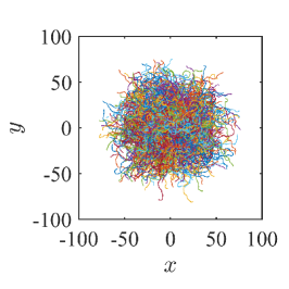
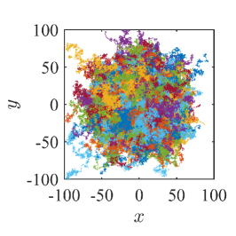
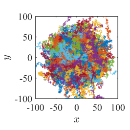
Figure 1: Trajectories of $N=1000$ simulated particles in two dimensions ($t=10\,\tau_{\phi}$). left: Micro-swimmer with inertia, Eq.(22); middle: Swimmer with random orientation and one stochastic force, Eq.(37); right: Swimmer with two independent stochastic forces, Eq.(46). Different colors show different trajectories. Parameters: $N=1000;v_{0}=1;D_{\phi}=0.1;dt=0.02$.

Beyond this time the motion of the micro-swimmer with constant speed becomes statistically indistinguishable from the motion of a Brownian particle. The difference is that the diffusion coefficient scales counter-intuitively with the intensity of the applied angular noise behaving as $D_{\mbox{\tiny{eff}}}\,\propto 1/D_{\phi}$ and decreasing when this intensity increases, whereas the normal diffusion enhances with increasing noise.

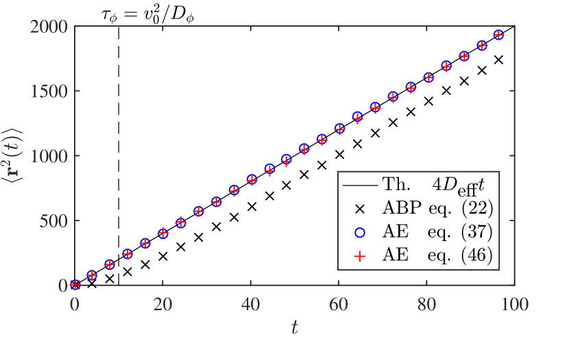
Figure 2: Simulated MSD in two dimensions: Comparison of the three different dynamics as labeled. The dashed line indicates the crossover time between the ballistic and the diffusive motion. Parameters are: $N=10000;v_{0}=1;D_{\phi}=0.1;dt=0.02$.

In Fig.1 we show sample paths for the two dimensional stochastic micro-swimmer with constant speed. The left graph shows the micro-swimmer with inertia (22), the middle graph the memoryless dynamics with random orientations according to (37). In the right graph trajectories are presented with two independent noise sources, corresponding to (46). Both approximations exhibit the same diffusive behavior where the diffusion coefficients converges to the asymptotic value of the case with inertia as presented in Fig.2. The mean square displacement of the latter one is smaller compared to the overdamped dynamics due to the initial ballistic growth.

3.5 Adiabatic elimination: Kinetic approach

In this section we derive the Smoluchowski equation of the micro-swimmer with constant speed following the kinetic approach in $\mathrm{Sec.}$ 2.2. The starting FPE for the joint transition probability density $P(\mathbf{r},\phi,t|\mathbf{r}_{0}=0,\phi_{0},t_{0})$ of the position $\mathbf{r}$ and orientation $\phi$ at time $t$ of the micro-swimmer with constant speed which has been started at $t_{0}$ in $\mathbf{r}_{0}$ with orientation $\phi_{0}$. It reads :

$$\frac{\partial\,P}{\partial\,t}\,\,=\,-\,v_{0}\,\frac{\partial\,}{\partial\,\mathbf{r}}\,\,\cdot\,\mathbf{e}_{v}\,P\,+\,\frac{D_{\phi}}{v_{0}^{2}}\,\frac{\partial^{2}}{\partial{\phi}^{2}}\,P.$$ (48)

We derive again transport equations for the zeroth, first and second moments of the orientation which are

$$\rho(\mathbf{r},t)\,=\,\int P(\mathbf{r},\phi,t)\,{\rm d}\phi\,,\leavevmode\nobreak\ \leavevmode\nobreak\ \leavevmode\nobreak\ \leavevmode\nobreak\ \leavevmode\nobreak\ \leavevmode\nobreak\ \rho(\mathbf{r},t)\,u_{i}(\mathbf{r},t)\,=\,v_{0}\,\int\,\mathbf{e}_{v_{i}}\,P(\mathbf{r},\phi,t)\,{\rm d}\phi\,,$$ (49)

$$\rho(\mathbf{r},t)\,\braket{\delta v_{i}\,\delta v_{j}}(\mathbf{r},t)\,=\,\int(v_{0}\,\mathbf{e}_{v_{i}}\,-\,u_{i}(x,t))(v_{0}\,\mathbf{e}_{v_{j}}\,-\,u_{j}(x,t))\,P(\mathbf{r},\phi,t)\,{\rm d}\phi.$$

Multiplication with zeroth, first and second powers of $\cos(\phi)$ and $\sin(\phi)$ and integration over $\phi$ results in the three transport equations

$$\frac{\partial\,\rho}{\partial\,t}\,+\frac{\partial\,}{\partial\,x_{k}}\,\rho\,u_{k}\,=0,\leavevmode\nobreak\ \leavevmode\nobreak\ \leavevmode\nobreak\ \leavevmode\nobreak\ \leavevmode\nobreak\ \leavevmode\nobreak\ \leavevmode\nobreak\ \leavevmode\nobreak\ \frac{\partial\,u_{i}}{\partial\,t}\,+u_{k}\frac{\partial\,u_{i}}{\partial\,x_{k}}\,=-\frac{D_{\phi}}{v_{0}^{2}}u_{i}-\frac{1}{\rho}\frac{\partial\,\rho\braket{\delta v_{i}\,\delta v_{k}}}{\partial\,x_{k}}\,,$$ (50)

$$\frac{\partial\,\braket{\delta v_{i}\,\delta v_{j}}}{\partial\,t}\,\,+\,u_{k}\frac{\partial\,\braket{\delta v_{i}\,\delta v_{j}}}{\partial\,x_{k}}\,\,=$$ (51)

$$\leavevmode\nobreak\ \leavevmode\nobreak\ \leavevmode\nobreak\ \leavevmode\nobreak\ \leavevmode\nobreak\ \leavevmode\nobreak\ \leavevmode\nobreak\ \leavevmode\nobreak\ \leavevmode\nobreak\ \leavevmode\nobreak\ \leavevmode\nobreak\ \leavevmode\nobreak\ \leavevmode\nobreak\ \leavevmode\nobreak\ =\,2\frac{D_{\phi}}{v_{0}^{2}}\left(v_{0}^{2}\delta_{i,j}\,-\,u_{i}\,u_{j}\,-\,2\,\braket{\delta v_{i}\,\delta v_{j}}\right)\,-\,\braket{\delta v_{i}\,\delta v_{k}}\frac{\partial\,u_{j}}{\partial\,x_{k}}\,\,-\,\braket{\delta v_{j}\,\delta v_{k}}\frac{\partial\,u_{i}}{\partial\,x_{k}}\,.$$

In these equations we can eliminate the first and second moments at times larger than the relaxation time $t\,\gg\,\tau_{\phi}$ assuming large noise $D_{\phi}$ or small velocities $v_{0}$. Since in this case the r.h.s of the corresponding balance equations are large, the substantial derivatives in their l.h.s. can be set to zero. From the equation for the variance $\braket{\delta v_{i}\,\delta v_{j}}$ we get

$$\braket{\delta v_{i}\,\delta v_{j}}\,\approx\,\frac{1}{2}\left(v_{0}^{2}\delta_{i,j}\,-\,u_{i}\,u_{j}\right)\,+\,O(\tau_{\phi})\,,\leavevmode\nobreak\ \leavevmode\nobreak\ \leavevmode\nobreak\ \leavevmode\nobreak\ \leavevmode\nobreak\ \leavevmode\nobreak\ \leavevmode\nobreak\ i,j\,=\,x,y.$$ (52)

where we assumed small variations of the mean velocities $\partial u_{i}/\partial x_{k}$ which would contribute to the variances in $O(\tau_{\phi})$ . The fact that the variance depends on the components of the mean velocity expresses the conservation of the mean kinetic energy (the kinetic energy of a particle moving at a constant speed is constant). This is clearly expressed by

$$u_{x}^{2}\,+\,u_{y}^{2}\,+\,\braket{(\delta v_{x})^{2}}+\,\braket{\delta v_{y})^{2}}\,=\,v_{0}^{2}.$$ (53)

The approximation (52) obeys this conservation law on the average. It represents a kind of equipartition of the kinetic energy between both degrees of freedom: each degree on the average obtains $v_{0}^{2}/2$. For the mixed components one gets correspondingly on the average $\,u_{x}\,u_{y}\,+\,\braket{\delta v_{x}\,\delta v_{y}}\,\approx\,0$.

Setting the l.h.s. to zero in the balance for the mean velocity results in

$$\rho\,u_{i}\,\approx\,-\,\frac{v_{0}^{2}}{D\phi}\,\frac{\partial\,}{\partial\,x_{k}}\,\,\braket{\delta v_{i}\,\delta v_{k}}\,\rho.$$ (54)

Insertion of Eq.(52) into Eq.(54) and of the resulting expression into the continuity equation finally gives

$$\frac{\partial\,\rho}{\partial\,t}\,=\frac{\tau_{\phi}}{2}\,v_{0}^{2}\,\left(\frac{\partial^{2}}{\partial x^{2}}+\frac{\partial^{2}}{\partial y^{2}}\right)\,\rho-\frac{\tau_{\phi}}{2}\left(\frac{\partial\,}{\partial\,x}\,u_{x}+\frac{\partial\,}{\partial\,y}\,u_{y}\right)^{2}\rho.$$ (55)

Eventually, we obtained the equation for the marginal probability density of the position $\rho(\mathbf{r},t)$ which is a valid approximation to characterize the dynamics of the micro-swimmer. So far still containing the mean velocity, it is not a closed description. Both terms are of linear order in $\tau_{\phi}$. However , we have to point out that the first one is multiplied by $v_{0}^{2}$ whereas the second one contains the components of the mean velocity $u_{x},u_{y}$. Though the mean velocities scale with the speed $v_{0}$, their values are much smaller than the constant speed if a sufficiently strong noise acts on the orientation. Neglecting in this situation consequently the second term in Eq. (55) yields the two -dimensional diffusion equation (47) with the constant diffusion coefficient (43). Its solution gives the expected approximation for $\rho(\mathbf{r},t)$. Otherwise, as always in cases where the motion is bounded by a maximal velocity, the diffusion approximation breaks down at the wings of the distribution. It happens in our case, when the mean velocity gets of the order of $v_{0}$.

4 Conclusions

We have been concerned with a stochastic micro-swimmer with constant speed and random orientation. This special type of an ABP performs ballistic motion at time scales smaller than the crossover time $\tau_{\phi}$ and exhibits normal diffusion at larger time scales. Our main purpose was to find an approach to an adiabatic elimination of the orientation of the velocity as a persistent variable, and to formulate a memoryless dynamics for the position of the particle in the diffusive regime. In analogy to the known theory of a normal Brownian particle which was revisited in Sec.2, we have derived in Sec.3 the overdamped dynamics of the projection of the motion onto a given direction (32) and also for the full two-dimensional case, Eq.(37). On the basis of stochastic differential equations we elaborated systematic elimination procedure. In addtion we propose a kinetic approach where we eliminate systematically the first and second spatio-temporal moments of the velocity and remain with the marginal density $\rho(\mathbf{r},t)$ to find the particle at time $t$ at position $\mathbf{r}$. In both approaches resulting equations still reflect important microscopic properties of the micro-swimmer as, for instance, the conservation of kinetic energy. Only after averaging over random orientations the particles loses this property and the description becomes similar to that of a normal overdamped Brownian particle.

Acknowledgements
The authors cordially congratulate Ulrike Feudel on occasion of her birthday and thank for a long-lasting friendship. This work was supported by the Deutsche Forschungsgemeinschaft via IRTG 1740.

Appendix A Angular Probability Density Function

The marginal probability density $P(\phi,t|\phi_{0},t_{0})$ of the orientation of active Brownian particles obeys the Smoluchowski equation. The latter can be obtained by integrating the FPE (48) over the position vector $\mathbf{r}$ which results in

$$\frac{\partial P(\phi,t|\phi_{0},t_{0})}{\partial t}=\frac{D_{\phi}}{v_{0}^{2}}\frac{\partial^{2}P(\phi,t|\phi_{0},t_{0})}{\partial\phi^{2}}.$$ (56)

For this parabolic equation the time-dependent solution for $2\pi$-periodic boundaries is known Tikhonov

$$P(\phi,t|\phi_{0},0)\,=\,\frac{1}{\pi}\left(\frac{1}{2}+\sum_{n=1}^{\infty}\cos[n(\phi-\phi_{0})]e^{-n^{2}\frac{D_{\phi}}{v^{2}_{0}}t}\right).$$ (57)

For $t\,\gg\,\tau_{\phi}{\color[rgb]{0,0,0}=v_{0}^{2}/D_{\phi}}$ the probability spreads homogeneously over the $[0,2\pi]$ interval:

$$P^{0}(\phi)\,=\,\frac{1}{2\pi}.$$ (58)

The characteristic time scale of the system is the relaxation time $\tau_{\phi}$ after which the first Fourier mode decays.

Appendix B Mean squared displacement of the stochastic micro-swimmer with constant speed

In 1997 Mikhailov and Meinköhn mikhailov derived the effective diffusion constant for the micro-swimmer with constant speed using the relation between the MSD and ACF (9) and using the solution of the Smoluchowski equation for the orientations given above in Appendix (A). Here we review their results shortly. The discussion is valid both in the ballistic and in the diffusive regime.

The mean square displacement can be calculated using (9) which for the micro-swimmer with constant speed explicitly reads

$$\langle\mathbf{r}^{2}(t)\rangle=v_{0}^{2}\int_{0}^{t}\int_{0}^{t}dt_{1}dt_{2}\langle\cos(\phi(t_{1})\,-\,\phi(t_{2}))\rangle.$$ (59)

Here $\phi(t_{1}),\phi(t_{2})$ are the orientations of motion at the two times $t_{1}$ and $t_{2}$, respectively, and the average has to be taken over their probability distribution, Eq.(57). Calculating the integrals leads to the result for the mean square displacement found by Mikhailov and Meinköhn:

$$\langle\mathbf{r}^{2}(t)\rangle=\frac{2v_{0}^{4}}{D_{\phi}}\,t\,+\,\frac{2\,v_{0}^{6}}{D_{\phi}^{2}}\,\left[\exp\left(\,-\,\frac{D_{\phi}t}{v_{0}^{2}}\right)\,-\,1\right]$$ (60)

Similarly to Eq.(3), it describes the ballistic and the diffusive behavior. For times $t\,\gg\,\tau_{\phi}$ the second term can be neglected and the MSD scales linearly in time with the diffusion coefficient given by Eq.(43). Linear growth in time is obtained at a coarse grained scale $|\mathbf{r}|\gg l_{\phi}=v_{0}\tau_{\phi}=v_{0}^{3}/D_{\phi}$.

References

- (1) H. Niwa, J. Theor. Biol. 171(2), 123 (1994).
- (2) T. Vicsek, A. Czirók, E. Ben-Jacob, I. Cohen, O. Shochet, Phys. Rev. Lett. 75(6), 1226 (1995).
- (3) P. Romanczuk, M. Bär, W. Ebeling, B. Lindner, L. Schimansky-Geier, Eur. Phys. J. Special Topics 202, 1 (2012).
- (4) M.C. Marchetti, J.F. Joanny, S. Ramaswamy, T.B. Liverpool, J. Prost, M. Rao, R.A. Simha, Rev. Mod. Phys. 85, 1143 (2013).
- (5) M.J.B. Hauser, L. Schimansky-Geier, Eur. Phys. J. Special Topics 224, 1147 (2015).
- (6) M. Schienbein, H. Gruler, Bull.Math.Biol. 55, 585 (1993).
- (7) S. van Teeffelen, H. Löwen, Phys. Rev. E 78(2), 020101 (2008).
- (8) D. Selmeczi, L. Li, L.I. Pedersen, S.F. Nørrelykke, P.H. Hagedorn, S. Mosler, N.B. Larsen, E.C. Cox, H. Flyvbjerg, Eur. Phys. J. Special Topics 157(1), 1 (2008).
- (9) H. Bödeker, C. Beta, T. Frank, E. Bodenschatz, Europhys. Lett. 90(2) (2010).
- (10) L. Li, S.F. Nørrelykke, E.C. Cox, PLoS ONE 3(5), e2093 (2008).
- (11) G. Amselem, M. Theves, A. Bae, E. Bodenschatz, C. Beta PLoS ONE 7(5) e37213 (2012).
- (12) R. Dilao, M.J.B. Hauser, Comptes Rendus Biologies 336(11-12), 565 (2013).
- (13) B. Rodiek and M.J.B.Hauser, Eur. Phys. J- Special Topics 224 1199 (2015).
- (14) S. Bazazi, P. Romanczuk, S. Thomas, L. Schimansky-Geier, J.J. Hale, G.A. Miller, G.A. Sword, S.J. Simpson, I.D. Couzin, Proc. R. Soc. B: Biol. Sci. (2010).
- (15) P Romanczuk, M. Romensky, D. Scholz, V. Lobaskin, and L. Schimansky-Geier, Eur. Phys. J- Special Topics 224 1215 (2015).
- (16) W.F. Paxton, K.C. Kistler, C.C. Olmeda, A. Sen, S.K.S. Angelo, Y. Cao, T.E. Mallouk, P.E. Lammert, V.H. Crespi, J. Am. Chem. Soc. 126(41), 13424 (2004).
- (17) J.R. Howse, R.A.L. Jones, A.J. Ryan, T. Gough, R. Vafabakhsh, R. Golestanian, Phys. Rev. Lett. 99(4), 048102 (2007).
- (18) G. Ruckner, R. Kapral, Phys. Rev. Lett. 98(15), 150603 (2007).
- (19) K.V. Kumar, S. Ramaswamy, M. Rao, Phys. Rev. E 77(2), 020102 (2008).
- (20) A. Kudrolli, G. Lumay, D. Volfson, L.S. Tsimring, Phys. Rev. Lett. 100(5), 058001 (2008).
- (21) P. Tierno, R. Albalat, F. Sagués, Small 6(16), 1749 (2010).
- (22) H. Ke, S. Ye, R.L. Carroll, K. Showalter, J. Phys. Chem. A 114(17), 5462 (2010).
- (23) D. Takagi, A. B. Braunschweig, J. Zhang, and M. J. Shelley, Phys. Rev. Lett. 110, 038301 (2013).
- (24) G. Grègoire and H. Chate, Phys. Rev. Lett. 92, 025702 (2004).
- (25) H. Chate, F. Ginelli, R. Montagne, Phys. Rev. Lett. 96(18), 180602 (2006).
- (26) J. Buhl, D.J.T. Sumpter, I.D. Couzin, J.J. Hale, E. Despland, E.R. Miller, S.J. Simpson, Science 312(5778), 1402 (2006).
- (27) E. Bertin, M. Droz, and G. Grègoire, Phys. Rev. E 74. 0222101 (2006).
- (28) T. Ihle, Phys. Rev. E 83, 030901 (R) (2011).
- (29) T. Ihle, Phys. Rev. E 88, 040303 (R) (2013).
- (30) R.Großmann, L. Schimansky-Geier and P. Romanczuk, Phys. Rev. Lett. 113 258104 (2014).
- (31) R. Großmann, F. Peruani and M. Bär, New Journal of Physics 18 043009 (2016).
- (32) H. Seyed-Allaei, L. Schimansky-Geier and M. R. Ejtehadi, Phys. Rev. E 94, 062603 (2016).
- (33) A. Patch, D. Yllanes, M.C. Marchetti, Phys. Rev. E 95, 012601 (2017).
- (34) F. Schweitzer, W. Ebeling, B. Tilch, Phys. Rev. Lett. 80, 5044 (1998).
- (35) F. Schweitzer, Brownian Agents and Active Particles: Collective Dynamics in the Natural and Social Sciences. Synergetics (Springer, 2003).
- (36) A. Mikhailov, D. Meinköhn, in Stochastic Dynamics, edited by L. Schimansky-Geier, T. Pöschel, Springer (1997).
- (37) F. Peruani and L.G. Morelli, Phys. Rev. Lett. 99, 10602 (2007).
- (38) P. Langevin, C. R. Acad. Sci (Paris) 146, 530 (1908).
- (39) P. M. Kareiva, and N. Shigesada, Oecologia 56, 234 (1983).
- (40) A. Okubo and S. A. Levin, Diffusion and Ecological Problems: Modern Developments,2nd edition, Interdisciplinary Applied Mathematics, vol. 14 (Springer Science + Business Media, New york, 2001).
- (41) W. Ebeling, F. Schweitzer, B. Tilch, Biosystems 49, 17 (1999).
- (42) U. Erdmann, W. Ebeling, L. Schimansky-Geier, F. Schweitzer, Eur. Phys. J. B 15, 105 (2000).
- (43) P. Romanczuk, L. Schimansky-Geier, Phys. Rev. Lett. 106, 230601 (2011).
- (44) F. J. Sevilla, L. A. Gomez Nava, Phys. Rev E 90, 022130 (2014).
- (45) H. A. Kramer, Physica 7, 284 (1940).
- (46) R. Becker,Theorie der Wärme (Springer, Berlin, 1955), chapter VI B.
- (47) Yu. B. Rumer, M. Sh. Rivkin, Thermodynamics, Statistical Physics and Kinetics, Mir Publishers Moscow (1980).
- (48) L. Haeggqwist, L.Schimansky-Geier, I.M. Sokolov, F. Moss, Eur.Phys.J. Spec.Top. 157(1), 33 (2008).
- (49) C. Weber, P. K. Radtke, L.Schimansky-Geier, and P. Hänggi, Phys. Rev. E 84, 011132 (2011).
- (50) C. Weber, I. M. Sokolov, and L. Schimansky-Geier, Phys. Rev. E 85, 052101 (2012).
- (51) F. Thiel, L. Schimansky-Geier, I.M. Sokolov, Phys. Rev. E 86, 021117 (2012).
- (52) J. Nötel, I. M. Sokolov and L. Schimansky-Geier, J. Phys. A: Math. Theor. 50, 034033 (2017).
- (53) M. Mijalkov, G. Volpe, Soft Matter, 9, 6376 (2013).
- (54) G. Volpe, S. Gigan, G. Volpe, Am. J. Phys. 82, 659 (2014).
- (55) A. Geiseler, P. Hänggi, F. Marchesoni, C. Mulhern, S. Savel’ev Phys. Rev. E 94, 012613 (2016).
- (56) A. Geiseler, P. Hänggi, P. Schmid, G. Eur. Phys. J. 89, 175 (2016).
- (57) D. Debnath, P.K. Ghosh, Y. Li, F. Marchesoni, B. Li, Soft Matter 12,2017 (2016).
- (58) B. ten Hagen, S. van Teeffelen, H. Löwen, J. Phys: Condensed Matter 23 194119 (2011).
- (59) S. Babel, B. ten Hagen, H. Löwen, J. Stat. Mech. P02011 (2014).
- (60) A. Einstein, Ann. Phys. 17(8), 549 (1905).
- (61) M. von Smoluchowski, Ann. Phys. 326(14), 756 (1906).
- (62) P. Hänggi, P. Talkner, M. Borkovec Rev. Mod. Phys. 62(2), 251 (1990).
- (63) L. H’walisz, P. Jung, P. Hänggi, P. Talkner, L. Schimansky-Geier, Z.Phys.B 77, 471 (1989).
- (64) H. Haken, Synergetics-an Introduction, 2nd ed. (Springer, Berlin, 1978), Chap. 7.
- (65) C. W. Gardiner, Handbook of Stochastic Methods(Springer, 1983).
- (66) C. W. Gardiner, Phys. Rev. A 29, 2814(1984).
- (67) P. Jung and P. Hänggi, Phys. Rev. A 35, 4464 (1987).
- (68) L. Schimansky-Geier and P. Talkner, in Stochastic Dynamics of Reacting Macromolecules, ed. by W. Ebeling, L. Schimansky-Geier, and Yu. M. Romanovsky, World Sientific, Singapore (2002).
- (69) J. M. Sancho, Phys. Rev. E 84, 062102 (2011).
- (70) R.L. Stratonovich, SIAM J. Control 4, 362 (1966); Topics in the Theory of Random Noise 1 (Gordon and Breach, New York 1963), pp. 89ff.
- (71) N. G. van Kampen, J. Stat. Phys 24, 175 (1981).
- (72) I.M. Sokolov, Chemical Physics 375, 359 (2010.
- (73) R. L. Stratonovich, in Noise in Nonlinear Dynamical Systems, ed. by F. Moss and P.V.E.McClintock, volume 1 (Cambridge University Press, 1989).
- (74) V. I. Tikhonov, M. A. Mironov, Markovian Processes(in Russian), (Soviet Radio, Moscow 1977).