Transit Timing Variations in the system Kepler-410Ab

Abstract

We present a new analysis of the transit timing variations displayed by the extrasolar planet Kepler-410Ab. We obtained and improved orbital and physical parameters for the planet and analysed 70 transit times obtained by the Kepler satellite. In our analysis of the O-C diagram (Observed-Calculated), we assumed that the observed changes in the transit times are probably caused by the gravitational influence of another body in the system. To determine the mass of the perturbing body, we have considered the light-time effect and an analytical approximation of the perturbation model. The solutions resulting from both methods give comparable results, with an orbital period $P_{3}\sim$970 days and a slightly eccentric orbit of the third body. We also showed that this orbit is nearly coplanar with the orbit of the Neptune-like planet Kepler-410Ab (orbital period 17.8 days). We propose two possible models for the perturbing body orbiting a common barycentre with Kepler-410A: (i) a single star with mass at least 0.906 M_☉, (ii) a binary star with the total mass of its components of at least 2.15 M_☉. In both cases the star Kepler-410B is on a long orbit (period more than 2200 years). Small amplitude variations ($\sim$ 5–8 minutes) detected in O-C residuals can be explained by the stellar activity of the host star (spots and pulsations), which affects the shape of the light curve during the transit. The presence of single or binary companion of mentioned masses heavily affects the total observed flux from the system. After removing of the flux contamination from Kepler-410A light curve we found that radius of the transiting planet Kepler-410Ab should be in the range from about 3.7 to 4.2 R_⊕.

1 Introduction

The Kepler mission, launched in 2009, has produced photometric data with unprecedented precision (Borucki et al., 2010). It was designed to detect Earth-size planets orbiting in the habitable zone of parent stars using the transit method. The Kepler spacecraft has revolutionized the study of exoplanets, variable stars and stellar astrophysics; providing photometric data with high-precision, high-cadence continuous light curves (LCs). After losing two reaction wheels, the Kepler spacecraft ended its primary mission and subsequently started its K2 mission started (Howell et al., 2014). The photometric precision of K2 is slightly lower, but still much better than that from ground-based observatories.

The high precision of Kepler data and the long-term uninterrupted observations enable us to determine not only transit parameters, but also to measure small changes in the individual times of transits with respect to a linear ephemeris that assumes a Keplerian orbit. These variations (often called Transit-Timing Variations, TTVs) can reflect dynamical interaction with other objects in the system (other star(s), planets(s)) which cannot be discovered directly by the transit method. Gravitational interactions between the non-transiting object and the transiting planet can cause a periodic shift of the star-planet barycentre which can be detected through changes in timings of transits (so called light-time effect). Alternatively, TTVs can also be caused by stellar activity when a surface spot deforms the shape of the transit which leads to systematic shifts in transit timing.

Up to now (24 February 2017), 2330 confirmed planets and 4706 planet candidates have been discovered by Kepler. Another 173 planets and 458 candidates have been detected during the K2 mission. One of the confirmed transiting exoplanets is Kepler-410Ab, a Neptune-sized planet on 17.8336 days orbit, discovered in 2013 and confirmed by Van Eylen et al. (2014). The host star Kepler-410A (KIC 8866102, KOI-42, HD 175289) is a young $2.76\pm 0.54$ Gyr old star with radius $1.352\pm 0.010$ R_☉ and mass $1.214\pm 0.033$ M_☉ and a spectral type F6IV (Molenda-Żakowicz et al., 2013). The first GAIA Data Release (Gaia Collaboration et al., 2016) gives a distance of $153.6^{+6.7}_{-6.1}$ pc.

Using adaptive optics, Adams et al. (2012) distinguished a small stellar companion Kepler-410B separated by an angular distance of $1^{\prime\prime}.63$. Van Eylen et al. (2014) found that this star is probably a red dwarf and ruled it out as a host star for the exoplanet.

TTVs of Kepler-410Ab were for the first time reported by Mazeh et al. (2013). They studied the TTVs using a sinusoidal model and found an O-C semi-amplitude of $13.91\pm 0.91$ minutes and a period of about 960 days. In a subsequent analysis, Van Eylen et al. (2014) used a ’zigzag’ model. They obtained a slightly larger semi-amplitude of 16.5 minutes, and a period of 957 days. They also noted that the shape of the O-C in not sinusoidal, which could be caused by an eccentric orbit of Kepler-410Ab.

In this paper we give a new analysis of the TTVs in the orbit of Kepler-410Ab. In Section 2, we describe the determination of the parameters of the exoplanet and the individual transit times of Kepler-410Ab. In the next Section 3, we provide the physical models used for fitting TTVs. Our results are discussed in Section 4.

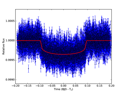
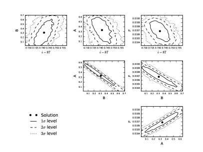
Figure 1: (top) – Stacked transits of Kepler-410Ab folded by the procedure described in Section 2. Original Kepler data are shown as blue points with error bars, the red line marks the best fit of the transit model with parameters in Tab. 1. (bottom) – Confidence interval graphs for fitted parameters (orbital inclination $i$, planet-star size ratio $p$ and limb darkening coefficients $A$ and $B$) determined by MCMC simulation.

Table 1: Transit parameters of exoplanet Kepler-410A determined for different flux contaminations of Kepler-410A light curve (see text), $a$ - semi-major axis of the planetary orbit (adopted from Van Eylen et al., 2014), $r_{\rm p}$ - planet radius, $i$ - orbital inclination, $A$, $B$ - linear and quadratic coefficients of the limb-darkening, $\chi^{2}$ - sum of squares of the best fit, $\chi^{2}/n$ - reduced sum of squares.

Parameter	Solution 1	Solution 2	Solution 3
Flux contamination	8%	42%	53%
	Kepler-410B	Kepler-410B+star	Kepler-410B+binary
$a$ [au]	0.1226$\pm$0.0047 a
$a$ [$R_{\star}$]	19.53$\pm$0.76 a
$r_{\rm p}$ [$R_{\earth}$]	2.647$\pm$0.020	3.744$\pm$0.029	4.239$\pm$0.033
$r_{\rm p}$ [$R_{\star}$]	0.01798$\pm$0.00004	0.02543$\pm$0.00006	0.02879$\pm$0.00006
$i$ [°]	87.744$\pm$0.003	87.745$\pm$0.003	87.745$\pm$0.003
$A$	0.3118$\pm$0.0404	0.3157$\pm$0.0421	0.3178$\pm$0.0450
$B$	0.3310$\pm$0.0457	0.3278$\pm$0.0488	0.3269$\pm$0.0492
$\chi^{2}$	33181.59	33214.11	33226.79
$\chi^{2}/n$	3.01	3.02	3.02
a adopted fixed value

2 Transit times determination

For the determination of the individual times of transit we used short-cadence (sampled every 58.8 seconds) de-trended data (PDCSAP_FLUX) from quarters Q1 to Q17, provided by the NASA Exoplanet Archive.

As a first step, we extracted parts of the LC around detected transits using the ephemeris given in Van Eylen et al. (2014), where we took an interval $\pm$0.2 days around the computed transit time $T_{\rm T}$ (the interval size is approximately double the transit duration). To remove additional residual trends caused by the stellar activity and instrumental long-term photometric variation, we fitted the out-of-transit part of LC by a second-order polynomial function. Then we subtracted 8% flux contamination from the wide companion Kepler-410B, according to calculations of Van Eylen et al. (2014) All individual parts of the LC with transits were stacked together to obtain the template of the transit. This can be done, because one expects that the physical parameters of the host star and the exoplanet did not change during the observational period of about 3.5 years and we want to cancel-out the effect of starspots.

The stacked LC was fitted by our software implementation of Mandel & Agol (2002) model, where we used the Markov Chain Monte Carlo (MCMC) simulation method for the determination of transit parameters. This method takes into account individual errors of Kepler observations and gives a realistic and statistically significant estimate of parameter errors. As a starting point for the MCMC fitting, we used the physical parameters of the planet given in Van Eylen et al. (2014). Because of the strong correlation between the orbital inclination $i$ and the semi-major axis $a$ of the planetary orbit, we have adopted a fixed value $a=0.1226\pm 0.0047$ au. We have used a quadratic model of limb darkening with starting values of coefficients (linear term $A$ and quadratic term $B$) from Sing (2010). We ran the MCMC simulation with 10⁶ steps. The convergence of MCMC fit was checked using the Geweke diagnostic (Geweke, 1992).

We have repeated the MCMC simulation with the previous solution as the starting point on each of 70 individual transit intervals, and let only the time of transit $T_{\rm T}$ to update. The new values of $T_{\rm T}$ were used to improve the linear ephemeris and to construct a new O-C diagram.

The combined light curve stacked using a linear ephemeris is affected by relatively large amplitude of O-C time shifts. To correct this effect, we used iterative procedure that takes the best-fit O-C values (see Section 3) into account. Afterwards, a new stacked light curve was constructed and a new MCMC transit solution was calculated, subsequently a new ephemeris and O-C values were determined. This process was repeated three times until a convergent solution was reached.

The resulting values of fitted transit parameter are listed in Tab. 1 (Solution 1). Corrected stacked transit light curve with the best fit is displayed in Fig. 1 (top) and confidence intervals of fitted parameters are displayed in Fig. 1 (bottom).

A new improved linear ephemeris was determined using obtained values of $T_{T}$ (Tab. 2):

$$T_{\rm T}=2455014.23765(22)+17.8336313(43)\times E,$$ (1)

where $E$ is the epoch of observation. Using the improved ephemeris (1), the corrected O-C diagram was constructed (Fig. 2).

3 Analysis of O-C diagram

Table 2: Barycentric transit times $T_{\rm T}$ of Kepler-410Ab, with their uncertainties $\sigma_{T_{\rm T}}$, $\chi^{2}$ and $\chi^{2}/n$ statistics ($n$ - the number of data points in the fit). The full table is available as a supplementary material to this manuscript.

$T_{\rm T}$ [BJD]	$\sigma_{T_{\rm T}}$	$\chi^{2}$	$\chi^{2}/n$	$n$
2454978.56473	0.00063	647.713	1.186	556
2454996.39755	0.00066	637.994	1.168	556
2455103.39002	0.00059	2509.821	4.709	543
2455121.22740	0.00069	2441.934	4.581	543
…	…	…	…	…

Our transit times $T_{\rm T}$ show a periodic variation with an amplitude of approximately 30 minutes and a period between 950 and 1000 days, which is in agreement with previous analyses by Mazeh et al. (2013) and Van Eylen et al. (2014).

Let us denote a linear ephemeris

$$\noindent T_{\rm C}=t_{\rm 0}+P\times E,$$ (2)

where $t_{\rm 0}$ is the initial time of transit, $P$ is the orbital period of the planet, and $E$ is the epoch of observation. The observed transit time $T_{\rm T}$ can be calculated by adding a perturbation $\delta T$ to the linear ephemeris (2):

$$T_{\rm T}=T_{\rm C}+\delta T.$$ (3)

Assuming that the observed TTVs are due to the gravitational influence of another body (planet or star) in the system, we can calculate $\delta T$ to find the physical parameters of the perturbing body using two different approaches:

1. LiTE (light-time effect) solution (Irwin, 1952). This method is often used to find an unseen companion in binary stars. A perturbation $\delta T$ caused by the third body is described by the equation:

   $$\delta T=\frac{a_{12}\sin i_{3}}{c}\left[\frac{1-e_{3}^{2}}{1+e_{3}\cos\nu_{3}}\sin(\nu_{3}+\omega_{3})+e_{3}\sin\omega_{3}\right],$$ (4)

   where $c$ is the speed of light, $a_{12}$ is semi-major axis of the orbit of Kepler-410A, and $i_{3}$, $e_{3}$, $\omega_{3}$, and $\nu_{3}$ are, respectively, the inclination, the eccentricity, the argument of the periastron, and the true anomaly of the orbit of the third-body around the barycentre of the system. Since the value of $i_{3}$ is not known, we can determine only the mass function for the third body:

   $$f(M_{3})=\frac{(M_{3}\sin i_{3})^{3}}{M^{2}}=\frac{(a_{12}\sin i_{3})^{3}}{P_{3}^{2}},$$ (5)

   where $M=M_{\star}+m+M_{3}$ is the total mass of the system (sum of the masses of the host star, the planet, and the third body, respectively). The minimal mass $M_{3}$ can be calculated by assuming a coplanar orbit, i.e. $i_{3}=i=87.\degr 74$. The period of the third body $P_{3}$ and the time of pericenter passage $t_{03}$ are hidden in the $\nu_{3}$ calculation and need to be solved for using the Kepler’s equation.
   

2. an analytical approximation of the perturbation model given in Agol et al. (2005). This method was originally developed for the analysis of multiple planetary systems, but is not constrained to any limit of mass of the perturbing body. An exterior body on a large eccentric coplanar orbit causes a time variation (eq. 25 in Agol et al. (2005)):

   $$\delta T= \frac{M_{3}}{2\pi(M_{\star}+m)}\frac{P^{2}}{P_{3}}(1-e_{3}^{2})^{-3/2}$$ (6)

   $$\left[\nu_{3}-n_{3}(t-t_{03})+e_{3}\sin\nu_{3}\right],$$

   where $n_{3}=2\pi/P_{3}$ is the mean motion. We can reduce the number of parameters in the model by substituting

   $$\frac{M_{3}}{M_{\star}+m}=\frac{\mu_{3}}{1-\mu_{3}}\ ,$$ (7)

   where $\mu_{3}=M_{3}/M$ is the reduced mass of the third body. Because the O-C amplitude is large, we expect the mass of the perturbing body to be of the order of one solar mass. Therefore, we can neglect the mass of the planet $m\ll M_{3}$.

To obtain the optimal parameters with statistically significant errors in both approaches, we have used our own code based on genetic algorithms for the determination of the initial values of all parameters, and MCMC simulation for the final solution and error estimation. The uncertainty of each individual $T_{\rm T}$ were considered. A full description of our code is in preparation (Gajdoš & Parimucha, 2017). The results from both methods are listed in Tab. 3 and depicted in Fig. 2 with confidence intervals shown in Fig. 3. To estimate the quality of the statistical model, we have also calculated the Bayesian information criterion (BIC) defined as:

$$\mathrm{BIC}=\chi^{2}+g\ln n$$

where $g$ is the number of degrees of freedom, and $n$ is the number of data points (TTVs). The lower BIC score means that a model is statistically more significant.

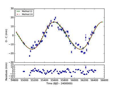
Figure 2: The O-C diagram of Kepler-410Ab constructed according to the improved linear ephemeris (1). The solid green line represents the best fit computed from the LiTE model, while the dashed red line corresponds to the solution according to the perturbation model by Agol et al. (2005). The residuals are plotted against the statistically better solution by the LiTE model.

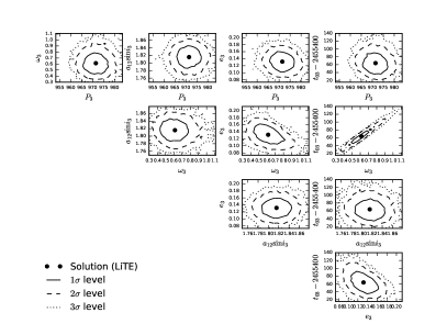
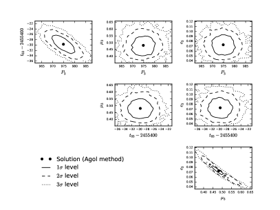
Figure 3: Confidence intervals determined by the MCMC simulation for parameters fitted in both methods.

4 Discussion and conclusion

Previous studies by Mazeh et al. (2013) and Van Eylen et al. (2014) dealt with only a quantitative analysis of TTVs in Kepler-410A system. The nature of the perturbing body was not discussed.

Our interpretation is based on a natural assumption that TTVs are caused by a gravitational influence of another body in the system. This is similar to period variations caused by a third body observed in eclipsing binaries.

It is obvious that a period of $\sim$970 days in the $O-C$ diagram cannot be caused by the companion star Kepler-410B. If we assume that this star is a low-mass (0.5-0.8 M_☉) cool star, based on the spectral type corresponding to the temperature $\sim 4850$ K derived by Van Eylen et al. (2014); and we take into account the observed separation ($1^{\prime\prime}.63$) and the distance to system (153.6 pc), we can calculate the orbital period of Kepler-410B to be in the range of 2200–2500 years.

The fact that the shape of the O-C diagram is not strictly sinusoidal (as first noted by Van Eylen et al. (2014)) agrees with our modelled eccentricity $e_{3}$ of the orbit of the third body. The orbital inclination $i_{3}$ cannot be determined directly from the O-C diagram. The analytical approximation of the perturbation model (Agol et al., 2005) assumes that the orbit is coplanar with that of the exoplanet and the planet is seen edge-on. These assumptions are valid, because the derived inclination of the planet is $i=87.\degr 74$.

To calculate the mass of the third body, we have neglected the mass of the planet $m\ll M_{3}$. According to the measured radius in the interval from $R_{p}=2.65\leavevmode\nobreak\ R_{\earth}$ to $R_{p}=4.24\leavevmode\nobreak\ R_{\earth}$ (see Tab. 1) the exoplanet Kepler-410Ab is a Neptune-like body and we can assume its mass of the order of several Neptune masses $m\sim 10^{-4}$ M_☉. The amplitude of the O-C curve is $\sim$30 minutes which is too high to be caused by a body with sub-stellar mass. The resulting mass of the third body $M_{3}=0.906\pm 0.155$ M_☉ should be regarded as a lower limit, because of the assumptions.

Table 3: Parameters of the third body obtained from two methods described in Section 3.

Parameter	LiTE solution	Agol method
$P_{3}$ [days]	971.1$\pm$3.7	973.6$\pm$3.6
$e_{3}$	0.15$\pm$0.02	0.09$\pm$0.01
$t_{03}$ [BJD]	2455440.2428$\pm$15.5311	2455372.1803$\pm$2.2120
$a_{12}\sin i_{3}$ [au]	1.839$\pm$0.020	–
$\omega_{3}$ [°]	25.8$\pm$5.8	–
$\mu_{3}$	–	0.428$\pm$0.041
$f(M_{3})$ [M☉]	0.879$\pm$0.030	–
$M_{3}$ [M☉]	2.151$\pm$0.078	0.906$\pm$0.155
$\chi^{2}$	804.9	831.5
$\chi^{2}/n$	12.4	12.6
BIC	826.2	848.5

Using the adopted LiTE solution, we arrived at the mass function (5) $f(M_{3})=0.879\pm 0.030$ M_☉. For a coplanar orbit (substituting $i$ for $i_{3}$) we get the minimal mass of the body $M_{3}=2.151\pm 0.078$ M_☉. If we consider a main-sequence star, this would correspond to the spectral type A4 (with $T_{\rm eff}\sim 8500$ K). But according to spectra obtained by Molenda-Żakowicz et al. (2013), the host star Kepler-410A is classified as F6IV. Moreover, during the $\sim$1460-days long observation by Kepler, no signs of eclipses with $\sim$970 days period were found. The mutual distance of bodies with masses $M_{\star}=1.2$ M_☉ and $M_{3}=2.1$ M_☉ orbiting with the period of $\sim$970 days is about 615 R_☉. For stars with radii $R_{\star}=1.35$ R_☉ (Van Eylen et al., 2014) and $R_{3}\sim 1.8$ R_☉ (according to assumed spectral type A4) eclipses will start to occur only if the inclination $i_{3}>89.\degr 87$, which explains the non-detection of additional transits. A more inclined orbit leads to more massive star with greater luminosity. This would favour the spectroscopic detection. However, if the perturbing body is comprised of a non-eclipsing binary star, the combined luminosity of both stellar components could still be under the detection limit of the spectrograph used by Molenda-Żakowicz et al. (2013).

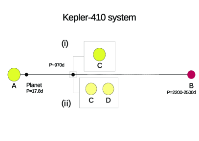
Figure 4: Schematic view of Kepler-410 system (not in scale). Planet b is orbiting the host star Kepler-410A with period 17.8 days, the orbital period of the companion star Kepler-410B is about 2200–2500 years, and the perturbing component (with orbital period relative to the system barycentre $\sim$970 days) could be: (i) a single star with minimal mass 1.12 M_☉, or (ii) a close binary star with the total mass of components at least 2.1 M_☉.

The light curve of Kepler-410A is affected by rotational flux modulation with the amplitude 7–8 mmag and the period about 25 days. The amplitude of exoplanet transits is only $\sim$4 mmag. To remove the signal of the modulation, we selected parts of LC with transits shorter than $\sim$0.2 days and fitted the out-of-transit part (see Section 2). The amplitude of O-C constructed with the updated ephemeris is about 30 minutes, which agrees with previous estimate by Van Eylen et al. (2014) and Mazeh et al. (2013). Some low-amplitude variations with periods in range of $\sim$ 200 days are still visible in residuals (Fig. 2). These can be interpreted by the presence of surface spots (Mazeh et al., 2015).

We propose the following scenarios to explain the observed TTVs in transits of Kepler-410A (see Fig. 4). The perturbing body is:

1. a star with minimum mass of 0.91 M_☉ in orbit around the common barycentre with Kepler-410A and the period $\sim$970 days.

2. a non-eclipsing binary star with minimum total mass of components 2.15 M_☉. The binary forms a hierarchical system with Kepler-410A.

In both cases, the component Kepler-410B is a cool red dwarf star on a distant orbit with period more than 2200 years and can not be the originator of observed TTVs.

We made simple N-body simulations of this problem for edge-on orbits. We used Everhart’s improvements of Gauss-Radau integrator (Everhart, 1985). Obtained O-Cs are very similar for both porposed scenarios. Any significant difference due to a possible binary character of perturbing compunent was not observed. The shape of model O-Cs (Fig. 2) was reproduced in our simulations. Based on our simulations, we could not explain the variations in the residuals to the O-C diagram. The oscillatory features of the residuals are not caused by possible binary character of perturbing compunent.

In both proposed scenarios we found different amounts of flux contamination by the perturbing body during the observed transits. If not corrected, the transit depth would be underestimated and the fit parameters would not accurate. We calculated possible minimum flux contamination using the mass-luminosity relation, from a single main sequence star with mass 0.91 M_☉ (Solution 2), and from a binary consisting of two main sequence stars with mass of each companion about 1M_☉ (Solution 3). The calculated contaminations were subtracted from Kepler-410A flux already corrected for a 8% Kepler-410B contribution (Van Eylen et al., 2014) and a new transit parameters were calculated using MCMC method (see Section 2). The results are listed in Tab. 1. Considering our proposed scenarios, the radius of the transiting planet Kepler-410Ab should be in the range from about $R_{p}$ = 3.74 R_⊕ to $R_{p}$=4.24 R_⊕. These values are significantly larger than that determined by Van Eylen et al. (2014). Other transit parameters as well as transit times were not affected by the correction to flux contamination.

Surprisingly, no systematic spectroscopic observations of this system are available to this date. In 2016, we started a low-dispersion spectroscopic campaign using a 60-cm telescope (Pribulla et al., 2015). Preliminary results suggest radial-velocity variations of Kepler-410A. For a definitive answer, we plan an observation program for high-dispersion spectroscopy of Kepler-410. Using the broadening-function method (Rucinski, 2002), we want to investigate the clues of radial velocities of any potential additional source.

Supporting information

Additional Supporting Information may be found in the on-line version of this article:

Table 2. Barycentric transit times $T_{\rm T}$ of Kepler-410Ab, with their uncertainties $\sigma_{T_{\rm T}}$, $\chi^{2}$ and $\chi^{2}/n$ statistics ($n$ - the number of data points in the fit).

Please note: Oxford University Press is not responsible for the content or functionality of any supporting materials supplied by the authors. Any queries (other than missing material) should be directed to the corresponding author for the paper.

References

- Adams et al. (2012) Adams, E. R. et al., 2012, AJ, 144, 42
- Agol et al. (2005) Agol, E. et al., 2005, MNRAS, 359, 567
- Borucki et al. (2010) Borucki, W. J. et al., 2010, Science, 327, 977
- Everhart (1985) Everhart E., 1985, An Efficient Integrator that Uses Gauss-Radau Spacings. Springer Netherlands, Dordrecht, 185–202
- Gaia Collaboration et al. (2016) Gaia Collaboration et al. et al., 2016, A&A, 595, A2
- Gajdoš & Parimucha (2017) Gajdoš, P., Parimucha, Š., 2017, in preparation
- Geweke (1992) Geweke J., 1992, In Bayesian Statistics. University Press, 169
- Howell et al. (2014) Howell, S. B. et al., 2014, PASP, 126, 398
- Irwin (1952) Irwin, J. B., 1952, ApJ, 116, 211
- Mandel & Agol (2002) Mandel, K., Agol, E., 2002, ApJ, 580, L171
- Mazeh et al. (2013) Mazeh, T., et al., 2013, ApJS, 208, 16
- Mazeh et al. (2015) Mazeh, T., Holczer, T., Shporer, A., 2015, ApJ, 800, 142
- Molenda-Żakowicz et al. (2013) Molenda-Żakowicz, J. et al., 2013, MNRAS, 434, 1422
- Pribulla et al. (2015) Pribulla, T., et al., 2015, AN, 336, 682
- Rucinski (2002) Rucinski, S. M., 2002, AJ, 124, 1746
- Sing (2010) Sing, D. K., 2010, A&A, 510, A21
- Van Eylen et al. (2014) Van Eylen, V. et al, 2014, ApJ, 782, 14