Conformal geodesics in spherically symmetric vacuum spacetimes with Cosmological constant
Abstract
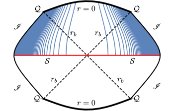
An analysis of conformal geodesics in the Schwarzschild-de Sitter and Schwarzschild-anti de Sitter families of spacetimes is given. For both families of spacetimes we show that initial data on a spacelike hypersurface can be given such that the congruence of conformal geodesics arising from this data cover the whole maximal extension of canonical conformal representations of the spacetimes without forming caustic points. For the Schwarzschild-de Sitter family, the resulting congruence can be used to obtain global conformal Gaussian systems of coordinates of the conformal representation. In the case of the Schwarzschild-anti de Sitter family, the natural parameter of the curves only covers a restricted time span so that these global conformal Gaussian systems do not exist.
1 Introduction
The purpose of this article is to analyse the behaviour of conformal geodesics in vacuum spherically symmetric spacetimes with a Cosmological constant. Conformal geodesics are a powerful tool for the analysis of global properties of spacetimes. In addition to their conformal invariance, their relevance stems from the fact that they single out privileged representatives of the conformal class of a solution to the Einstein field equations. General properties of conformal geodesics in the context of General Relativity have been studied in [7, 6]. In particular, in the later reference it has been shown that for the Schwarzschild spacetime it is possible to construct a non-singular congruence of conformal geodesics covering the whole of the Kruskal-Székeres maximal extension of the spacetime. This congruence can be used, in turn, to construct a conformal Gaussian gauge system consisting of a system of coordinates and an adapted frame which are suitably propagated off a fiduciary hypersurface in the spacetime. The construction and analysis of the properties of this class of gauge systems can be regarded as a basic first step towards the analysis, by means of conformal methods, of generic spacetimes with a global structure similar to that of the Schwarzschild spacetime. The use of conformal Gaussian systems in conjunction with the conformal Einstein field equations renders a particularly attractive system of evolution equations for which all the conformal fields, save for the Weyl tensor, satisfy mere transport equations along the conformal geodesics —see e.g. [4, 5, 17].
The main result of our analysis is that, as in the case of the Schwarzschild spacetime, it is possible to construct congruences of conformal geodesics covering the maximal extensions of the subextremal and extremal Schwarzschild-de Sitter (SdS) solutions. These congruences allow, in turn, to construct global systems of conformal Gaussian coordinates. For the case of the Schwarzschild-anti de Sitter (SadS) spacetime, the situation is more subtle: although the congruence of conformal geodesics covers the whole of the maximal extension of the spacetime, the natural parameter of the curves of the congruence only describes a portion of the time span of the curves. A similar phenomenon has been observed in the anti de Sitter spacetime —see [4].
Applications of the constructions described in this article to the analysis of more general (i.e. non-symmetric) classes of vacuum spacetimes in the case of a de Sitter-Like Cosmological constant are given elsewhere —see [8].
Notations and conventions
In what follows will denote spacetime abstract tensorial indices, while are spatial tensorial indices ranging from 1 to 3. By contrast, and will correspond, respectively, to spacetime and spatial coordinate indices.
The signature convention for spacetime metrics is . Thus, the induced metrics on spacelike hypersurfaces are negative definite.
An index-free notation will be often used. Given a 1-form and a vector , we denote the action of on by . Furthermore, and denote, respectively, the contravariant version of and the covariant version of (raising and lowering of indices) with respect to a given Lorentzian metric. This notation can be extended to tensors of higher rank (raising and lowering of all the tensorial indices). The conventions for the curvature tensors will fixed by the relation
2 The Schwarzschild-de Sitter and Schwarzschild-anti de Sitter spacetimes
In the remaining of this article we will be concerned with the analysis of spherically symmetric spacetimes satisfying the vacuum Einstein equations with Cosmological constant
| (1) |
In the previous expression, and denote, respectively, the Ricci tensor and the Ricci scalar of the metric . It follows that
The minus sign in front of the Cosmological constant in equation (1) has been chosen to ensure that corresponds to de Sitter-like spacetimes while is associated to anti de Sitter-like spacetimes. The assumption of spherical symmetry dramatically reduces the number of solutions to the field equations (1). Indeed, a generalisation of Birkhoff’s theorem shows that the only spherically symmetric solutions to the vacuum Einstein field equations with Cosmological constant are the Schwarzschild-de Sitter, the Schwarzschild-anti de Sitter and the Nariai solutions —see [16].
The line element of the Schwarzschild-de Sitter and Schwarzschild-anti de Sitter spacetimes is given, in standard coordinates , by
| (2) |
where
is the standard metric of and
In the conventions used in this article, the case corresponds to the Schwarzschild-de Sitter spacetime and the case to the Schwarzschild-anti de Sitter spacetime. In what follows, to simplify the computations we perform a rescaling of the line element in (2) so as to obtain the expression
| (3) |
The constant takes the value for Schwarzschild-de Sitter case and for the Schwarzschild-anti de Sitter case —hence, is always kept strictly positive. It is convenient to define
| (4) |
Note that in the representation given by the line element (3) both and are dimensionless quantities —this corresponds to a choice of units in which , hence the Cosmological constant is also dimensionless.
In the sequel, it will be necessary to make use of alternative coordinate systems for the metric . In particular, an isotropic radial coordinate can be introduced by means of the relations
| (5) |
so that the metric line element in equation (3) transforms into
The explicit form of the function is not needed in our computations. In addition, we also make use of Eddington-Finkelstein null coordinates defined by the relations
| (6) |
where is the tortoise coordinate defined via
| (7) |
the constant of integration in the last expression is usually to be chosen so that
consequently . Following standard conventions we refer to as the retarded null coordinate while is the advanced null coordinate. These coordinates render the line elements
2.1 Specific properties of the Schwarzschild-de Sitter spacetime
In this Section the Schwarzschild-de Sitter case is analysed, consequently will be assumed. Observe that, for , the function can be rewritten as
| (8) |
where and are two different positive real roots, and a is a negative real. Moreover, one has that
| (9) |
The root corresponds to a black hole-type horizon, while the root is associated to a Cosmological de Sitter-like horizon. It can be readily verified that for while for and . Consequently, the metric is static in the region between the two horizons and there are no other static regions outside this range for . Using Cardano’s formula for cubic equations it is possible to find the explicit values of , and . One finds that
| (10a) | |||
| (10b) | |||
| (10c) | |||
where the parameter is defined through the relation
| (11) |
We will refer to this case, for which , as the subextremal Schwarzschild de-Sitter spacetime. In contrast, the case for which will be referred as the extremal Schwarzschild de-Sitter spacetime. This is of special interest as one has
so that the function takes the form
| (12) |
Finally, it is observed that one can also consider the hyperextremal Schwarzschild de-Sitter spacetime characterised by the condition . In this case, the spacetime does not contain horizons.
2.2 Specific properties of the Schwarzschild anti de Sitter spacetime
For the Schwarzschild-anti de Sitter spacetime , consequently, in this case, the function has a single real root . Using Cardano’s formula one finds that
| (13) |
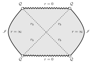
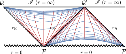
The root is associated to an event horizon separating two regions: a black hole region with a singularity at and an exterior region defined by the condition where the spacetime is static —see Figure 3. One can eliminate the parameter in equation (13) and write in terms of as
| (14) |
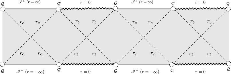
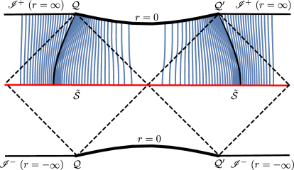
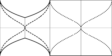
2.3 Penrose diagrams
The Penrose diagrams of the Schwarzschild-de Sitter and the Schwarzschild-anti de Sitter spacetimes are well known —see e.g., [9] for details on their construction. These diagrams are given in Figures 1-3. A discussion of the general procedure for the construction of Penrose diagrams in spherically symmetric spacetimes can be found in [17], Chapter 6.
3 Conformal geodesics in vacuum spacetimes with Cosmological constant
In this Section some basic results concerning conformal geodesics in vacuum spacetimes are briefly reviewed. Full details can be found in [4, 6, 14] —see also [17]. In what follows, let denote a spacetime satisfying the vacuum Einstein field equations with Cosmological constant (1).
3.1 Basic definitions
Given an interval , let , denote a curve in and let denote a 1-form along . Furthermore, let denote the tangent vector field of the curve . The conformal geodesic equations are then given by:
| (15a) | |||
| (15b) | |||
where denotes the Levi-Civita connection of the physical metric and denotes a derivative in the direction of . Notice that in the last expression the indices of the vectors and covectors are raised or lowered using —unless otherwise stated, we follow this convention in the rest of this article. The symbol denotes the Schouten tensor of defined by:
In the case of a spacetime satisfying the vacuum equations with Cosmological constant (1) one has that:
| (16) |
In the remainder of this article it is assumed that the spacetime satisfies condition (16).
3.2 Conformal factors along conformal geodesics
Conformal geodesics allow to single out a canonical representative of the conformal class of . Let denote a conformal extension of . Hence, there exists a scalar such that the metrics and are related via
| (17) |
The conformal factor can be fixed by requiring to be timelike and imposing the normalisation condition
| (18) |
Using equation (16), repeated differentiation of condition (18) together with the conformal geodesic equations and the Einstein field equations expressed as in equation (16) one obtains the relations
where , etc. Integrating the last of these equations along a given conformal geodesic one finds
| (19) |
where , and are prescribed at a fiduciary value of the parameter along the conformal geodesic . The coefficients and satisfy the constraints
| (20) |
where and denote, respectively, the value of and at . A further computation exploiting the above expressions shows that
Thus, as it is well known for vacuum spacetimes, the causal character of the conformal boundary is determined by the sign of —spacelike if and timelike if .
Remark 1.
Notice that by virtue of the normalisation condition (18), is the -proper time of the conformal geodesic.
3.3 The -adapted equations
In specific computations, it is more convenient to consider a parametrisation of the conformal geodesics in terms of the physical proper time. To this end, consider the parameter transformation given by
| (21) |
with inverse . In what follows, let . Using this notation, it can then be verified that
| (22) |
and that
so that is the -proper time of the curve . In order to write the equation for the curve in a convenient way, we consider the split
| (23) |
where the 1-form satisfies
Moreover one can verify that
| (24) |
In terms of these objects the -adapted equations for the conformal curves are given by
| (25a) | |||
| (25b) | |||
where
| (26) |
is constant along a given conformal geodesic.
3.4 The deviation equations
When working with congruences of conformal geodesics it is important to analyse whether they develop conjugate points. To this end, let and denote a family of conformal curves depending smoothly on a parameter . Following [6], let
The fields and denote, respectively, the deviation vector field and the deviation 1-form. The conformal Jacobi equation and the 1-form deviation equation are given by
| (27a) | |||
| (27b) | |||
where denotes the Riemann tensor of the metric , and
A -adapted version of the conformal geodesics can be readily computed. Accordingly, let be a reparametrisation of in terms of the physical proper time . Moreover, let
In terms of these new variables one has that equations (27a)-(27b) take the form
| (28a) | |||
| (28b) | |||
A computation shows that
Therefore, is constant along a given conformal geodesic.
3.5 Formulae in warped product spaces
The line element (2) is in the form of a warped product. This structure can be exploited to simplify the analysis of the -adapted conformal geodesic equations (25a)-(25b). To have a self-contained discussion, the main formulae for warped product spacetimes, originally derived in [6], are given in this Section.
In what follows, the discussion will be particularised to spacetimes whose metric can be written in the warped product form:
| (29) |
with
and and . In addition, it is assumed that the 2-dimensional metric given by is Lorentzian, while is a negative-definite 2-dimensional Riemannian metric. In view of this structure it is natural to consider solutions to the conformal curve equations satisfying and . In the case of the metric given by the line element (2) this Ansatz leads to solutions to the conformal curves which have no evolution on the angular coordinates, and one has only to consider evolution equations for the coordinates —or alternatively or . A direct computation shows that for this type of conformal geodesics the -adapted equations for the conformal geodesics imply
| (30a) | |||
| (30b) | |||
with
denoting the volume form of and where denotes the Levi-Civita covariant derivative of . A further computation shows that under the present Ansatz, the -adapted deviation equations (28a)-(28b) are equivalent to each other and to the equation
| (31) |
where denotes the Ricci scalar of .
For conformal curves satisfying and , the question of whether the deviation vector field is non-vanishing can be rephrased in terms of a similar question for the scalar
| (32) |
Notice that as long as , and are linearly independent. A computation using the deviation equation (31) yields
| (33) |
If we regard the congruence of conformal geodesics as a congruence in a conformal extension with then the scalar which we need to analyse is
| (34) |
where . The scalar has a similar geometric meaning as for the congruence of conformal geodesics regarded as curves in the unphysical spacetime. From equation (22) we deduce that and in addition . Hence
| (35) |
3.6 Explicit expressions for the reduced conformal geodesic equations
The corresponding 2-dimensional metric , as determined by the warped product form (29), for the line element of equation (3), is given by
| (36) |
It follows that the reduced conformal geodesic equations (30a)-(30b) reduce to
| (37a) | |||
| (37b) | |||
where consistent with the notation of Section 3.3 we have set and . Initial data for these equations can be prescribed following the discussion of Sections 3.1-3.3. Observe that equations (37a)-(37b) can be decoupled by making use of the -normalisation condition
| (38) |
Solving the latter for and substituting into equation (37b), one obtains that
| (39) |
This equation can be integrated once to yield
where is a constant given in terms of the initial value of the radial coordinate by
| (40) |
It follows that
| (41) |
with the sign depending on the value of . Substituting the latter expression into equation (38) we get
| (42) |
Remark 2.
As a notational remark we stress that is only used as a variable for integration. Notice, in contrast, that and represent the and proper time.
The solutions of equations (41) and (42), or equivalently expressions (43a) and (43b), completely determine and which in turn imply a congruence of conformal geodesics. Observe that, the coordinate is not well defined at the cosmological and black hole horizons, located at and , respectively. Therefore, to describe a conformal geodesic crossing the horizons it is necessary to replace by either or ; the retarded and advanced null coordinates defined in equation (6). The -normalisation condition in the and coordinates is written as
| (44) |
respectively. The normalisation condition (44) renders
| (45) |
3.7 Explicit expressions for the reduced conformal deviation equations
A direct calculation shows that if the Lorentzian metric has the form of equation (36) then
Therefore, equation (33) takes the form
| (47) |
In order to derive initial data for it is necessary to specify the initial data for the deviation vector . To do so, first observe that we can parametrise the congruence as where determines the intersection of the curve with the initial hypersurface . Alternatively, considering an approach similar to the one used in [14] we can make use of the standard isotropic coordinate defined by the relations in (5) and use to parametrise the congruence. This approach leads to the choice for the initial data for the deviation vector. Accordingly, we consider equation (47) with the choice . Consistent with this choice equation (47) reads
| (48) |
where . The solution of this equation will be determined once the initial conditions and have been prescribed and the corresponding value of replaced.
4 Analysis of the conformal geodesics in the subextremal Schwarzschild-de Sitter case
In accordance with the discussion of Section 2.1, for the subextremal Schwarzschild-de Sitter spacetime it is assumed that and . In this case one expects to be able to construct a congruence of conformal geodesics which combines characteristics of analogous congruences in the de Sitter and Schwarzschild spacetime.
4.1 Basic setup
The de Sitter spacetime can be covered by a congruence of conformal geodesics which have no initial acceleration —see [13, 17]. Based on this result we consider as initial hypersurface the time symmetric slice and require the conformal geodesics to be orthogonal to —see Figure 5. Exploiting the periodicity of the spacetime, it is sufficient to restrict the analysis to initial data in the range
If then we consider initial data for the congruence of conformal geodesics of the form
| (51) |
so that the tangent vector coincides with the future unit normal to . It follows that in this case so that the resulting congruence of conformal geodesics is, after reparametrisation, a congruence of metric geodesics. Metric geodesics in the Schwarzschild-de Sitter spacetime have been studied in the literature —see [10]. For completeness, we here we carry out an independent analysis adapted to the present setting. Observe that equation (41) together with the condition readily yields
| (52) |
Using the latter one can write
| (53) |
For convenience of the subsequent discussion we introduce the polynomial
with
If then the last three conditions in equation (51) can be still regarded a valid initial data but not the conditions involving . The cases and and will be discussed in Sections 4.2.4 and 4.2.5. It is convenient to define
The role of will be clarified Section 4.2.1. An immediate observation regarding the location of is the content of the following lemma.
Lemma 1.
For one has that
Proof.
In the parametrisation introduced in equation (11) we have
In addition, if one has the inequalities
∎
Remark 3.
Observe that in the extremal case one has consequently where denotes the location of the Killing horizon.
Given that has been chosen to be orthogonal to and the range of is bounded, we can set
To simplify the subsequent expressions recall from Section 2 that one can set with in the case of a de-Sitter like Cosmological constant. Consistent with this choice, equations (19)-(20) render
| (54) |
From this expression one can determine the relation between and using equation (21). A calculation gives
| (55) |
Observe that
so that the conformal boundary is reached in a finite value of the unphysical proper time .
Remark 4.
The coordinate is not well-defined at the points where vanishes. In the subextremal case, this corresponds to the Cosmological and black hole horizons while in the extremal case this corresponds to the Killing horizon.
To analyse the geodesics crossing the horizon one has to parametrise the curve in terms of the coordinates or , where and are advanced and retarded null coordinates. Setting equations (45) and (41) render
| (56) |
Choosing the second sign in equation (56) and using L’Hôpital rule one finds
| (57) |
Similarly, choosing the first sign in equation (56) one gets
| (58) |
Therefore, one can use the coordinates to describe the curves crossing the Cosmological horizon at . Similarly, the coordinates can be used to analyse curves crossing the black hole horizon at .
4.2 Qualitative analysis of the behaviour of the curves
In this Section we analyse the different qualitative behaviours of the conformal geodesics defined by the initial conditions introduced in the previous Section. As it will be seen, in broad terms, there are three types of conformal geodesics: those that escape to the asymptotic points, those that escape to the conformal boundary and those falling into the singularity.
4.2.1 Conformal geodesics with constant (critical curve).
In this Section we discuss whether it is possible to have conformal geodesics for which is constant. Substituting the conditions in equation (39) one readily obtains the condition
The latter implies
| (59) |
The curve will be called the critical curve.
Remark 5.
Notice that the curve never crosses the horizon since by virtue of Lemma 1 one has . For this curves is always finite and they approach one of the asymptotic points or .
In addition, one has the following result:
Lemma 2.
Assume and , then one has the chain of inequalities
Proof.
To prove this result it is convenient to write in terms of . One finds that
| (60) |
From the previous relation it is clear that and that . If then
| (61) |
which entails . Also for any we have
| (62) |
If we set in the last inequality and use the inequality (61) we deduce . This proves the second chain of inequalities. Assume now that . Then
| (63) |
which entails . If then
| (64) |
Using equation (42) and the initial data one readily finds that along the critical curve
Hence, as . Alternatively, using formula (55), one can express in terms of the unphysical proper time. One obtains
| (65) |
To complete the discussion observe that that along the critical curve one has , so that along the critical curve is a constant. Using equations (6) and (65) one concludes that along the critical curve
thus at where vanishes, one has and .
Asymptotic behaviour of the critical curve. In the rest of this Section we will analyse more closely the behaviour of the critical curve. Exploiting the above notation and using the initial data (51), the integral (43a) can be then rewritten as
| (66) |
To study the behaviour close to the critical curve consider . For small and one can expand the right hand side of equation (66) in Taylor series as
| (67) |
Integrating we obtain
As expected, the last expression diverges as . The divergent term can be expanded for small as
and the second term can be expanded as
Hence, to leading order one has
where
Rewriting the last expression in terms of the unphysical proper time using equation (55) one has, to leading order, that
| (68) |
where . Differentiating we get
Since then one has that diverges as . Consequently, the critical curve becomes tangent to the horizon as it approaches the asymptotic points and . In other words, the critical curve becomes null asymptotically. This behaviour is similar to that observed in the Schwarzschild spacetime where plays the role of timelike infinity as discussed in [5] and the subextremal Reissner-Nordström spacetime in [14].
Remark 6.
The change in the the causal behaviour of the critical curve discussed in the previous Section is evidence of the strong singular behaviour of the conformal structure at the asymptotic points.
4.2.2 Conformal geodesics with
Direct evaluation of equation (39) at for shows that . As one has that is a local minimum of . Hence, the curves with have initially increasing —i.e . Accordingly, making use of the relations see equations (52) and(53) one is led to analyse the ordinary differential equation
| (69) |
Making use of Lemma 2 one sees that the turning points of the equation are located at a value of which is smaller than . As is initially increasing it follows then that for . Moreover, as it follows that for . Finally, from equation (69) it follows that for the initial data under consideration if and only if . It only remains to be checked that (or ) do not blow up in a finite amount of physical proper time . From equation (69) the physical proper time is given by
| (70) |
According to Lemma 2 if one has that . Then, for any it holds that . Given that we have
Therefore the integral (70) is real for any . In addition, one has that
Thus
Hence
showing that does not blow up in finite physical proper time.
Remark 7.
Summarising, the analysis in the previous paragraphs shows that if , then as .
As discussed in a remark given in Section 4.1 the coordinate is not well behaved at the horizon. To follow the curves crossing the Cosmological horizon at one needs to use null coordinates . In the following we first show that along the conformal geodesics the coordinate remains well defined for any finite value of , in particular, for . Then, we show that is finite at the conformal boundary. As discussed in Section 4.1 it is enough to analyse equation (46a) choosing the second sign so that . To start the discussion observe that the coordinate is determined by integration of equation (46a) by
| (71) |
Analysis for the region with . Observe that, by continuity, one has that for would diverge if and only if the derivative diverges for some . Direct inspection of equation (46a) using expressions (8), (9) and (53) show that is finite for . Thus it only remains to compute the limit
Choosing the second sign in equation (46a) and rearranging one has
| (72) |
A direct application of the L’Hôpital rule shows that
Consequently does not diverge for . In other words
| (73) |
for some constant .
Analysis for the region with . First let us found an appropriate estimate for the integral (71) for and show that the coordinate acquires a finite value at . Using that for , we observe that
| (74) |
Recall that according to the initial data given in Section 4.1 one has . Exploiting the last observation we find an estimate for as follows:
| (75) |
To estimate the last integral of expression (75) observe that inequality (74) can be written as equivalently
thus
Using again inequality (74), written as and taking into account that , we get the following
Following the last chain of inequalities one can estimate the integral (75) as follows
| (76) |
Using equation (10c) and the triangle inequality one can verify that the location of the cosmological horizon is constrained by
Now, consider
and let . Using this notation we can estimate as follows
| (77) |
In the last inequality we have used equation (74), in the form . Using the functional form for in the subextremal case, one has that, for
Consequently,
Integrating the last inequality we get
Thus,
| (78) |
| (80) |
Remark 8.
Summarising, the analysis in the previous paragraphs shows that the conformal geodesics with cross the Cosmological horizon at and eventually escape to the conformal boundary. In particular, the curves do not touch the asymptotic points and for which and .
4.2.3 Conformal geodesics with
Direct evaluation of equation (39) at for shows that so that is a local maximum of —that is, . Hence, the curves with have initially decreasing and one has
From the above relation we deduce that the proper time of the curves is given by
| (81) |
Lemma 2 tells us that if one has that and therefore for any it holds that . Hence implies that
This means that the integrand in equation (81) is real for any in . In addition, one has that
Consequently, one can conclude that
This means that remains finite for any value of in the interval . In particular the geodesics reach the singularity in a finite value of the proper time .
Behaviour across the black hole horizon at . To complete the discussion of this class of conformal geodesics we now show that the advanced time coordinate can be used to follow the curves across the horizon at and that the value of remains finite as . Given that is finite at —cf. the limit in equation (58)— it follows that the coordinate has a finite value at . Moreover, it can be readily verified that
Thus, the coordinate acquires a finite limit as .
Remark 9.
Summarising, the conformal geodesics with reach the black hole horizon at in a finite amount of proper time and fall into the singularity at also in a finite proper time. Further, the curves remain away from the asymptotic points and for which and .
4.2.4 Conformal geodesics through the bifurcation sphere of the cosmological horizon
As shown in previous Sections the conformal geodesics with initial data arrive at the conformal boundary at a finite value of the unphysical proper time . However it is possible that the conformal geodesics accumulate in certain region of . In order to see that this is not the case we analyse the behaviour of the conformal geodesics starting at the bifurcation sphere of the horizon at .
In order to proceed with the analysis, it is convenient to introduce Kruskal type coordinates. First, recall that the Schwarzschild-de Sitter metric can be written as
where the induced metric on the quotient manifold as defined in equation (36). Introducing Kruskal coordinates via
where and are the Eddington-Finkelstein null coordinates as defined in equation (6) and is a constant which can be freely chosen. In this coordinate system the metric reads
with
where is the tortoise coordinate as defined in equation (7). A straightforward computation using (8) taking into account that renders
| (82) |
One can verify that and that
| (83) |
where are constants defined via
As discussed in [1] one cannot construct coordinates that are regular in the neighbourhood of the Cosmological and black hole horizons simultaneously. Since in this Section we are only interested in analysing the conformal geodesic starting at we observe that setting
so that , one gets
Introducing a further change of coordinates and one obtains
| (84) |
where the coordinates and are related to and via
| (85) |
A straightforward computation renders the additional relation
| (86) |
with and . Observe that the metric (84) is regular at . Moreover, notice that, since
and then
Consequently, the conformal geodesic starting at the bifurcation sphere in these coordinates correspond to the geodesic with initial position . Consistent with the discussion of Sections 3.5-4.1 we consider curves with no evolution in the angular coordinates and , so in these coordinates, the geodesic equations read
| (87) | |||
| (88) |
where as before ′ denotes a derivative respect to the physical proper time . Now, consider the curve with initial conditions
| (89) |
and recall that in the asymptotic region the curves with constant approach the bifurcation sphere —see Figure 4. Moreover, observe that in the -coordinate system the curve with is described by and . In the subsequent discussion we show that this curve is the required geodesic with the initial data given in equation (89). Assuming equations (87) render the conditions
| (90) | |||
| (91) |
Observe that equation (90) can be rewritten as an equation for while equation (91) has to be verified with the implicit expression for . Using the chain rule we have
Using the implicit function theorem and equation (86) one can compute to obtain
Notice that and while vanishes for as long as . Since one concludes that equation (91) is satisfied. To verify that this curve corresponds also the geodesic with initial data (89) observe that using the chain rule and the definition of the tortoise coordinate one has
| (92) |
Since at one has then
To analyse this limit observe that
Using equations (41) and (53) with and one has
where
substituting equation (8) one obtains
Evaluating the last expression at and using equation (92) one concludes that . Moreover one can verify that is positive and finite. Finally, notice that
Remark 10.
The analysis in the previous paragraphs shows that conformal geodesics with intersect the conformal boundary at . In terms of the retarded Eddington-Finkelstein null coordinate this corresponds to the condition . Accordingly, these conformal geodesics bisect the Cosmological region of the spacetime, and in particular also the conformal boundary.
4.2.5 Conformal geodesic through the bifurcation sphere of the black hole horizon
The analysis of the previous Section can be adapted, mutatis mutandi, to the case of conformal geodesics starting at . In this case the function in the function as given by equation (83) is set to
so that
As and given that , it follows that
Using the same methods employed in the analysis of the geodesics with , it can be readily shown that the curves with initial conditions given by
and such that
are conformal geodesics. Moreover, it can be verified that
In what follows, we will denote by the value of the null coordinates associated to . Notice that, in particular .
Remark 11.
The analysis of the previous paragraphs shows that the black hole region is bisected by timelike conformal geodesics emanating from the bifurcation sphere at .
4.3 Explicit expressions in terms of elliptic functions
The integral of equation (43a) can be written in terms of special functions. In particular, using formulae 258.13 and 339.01 given in [2], with parameters
one can rewrite the integral (66) in terms of elliptic functions. Using these formulae one concludes that the substitution
leads to
| (93) |
where sn denotes the Jacobian elliptic function, is the incomplete elliptic integral of the third kind and
In particular, it follows from the previous expressions and the general theory of elliptic functions that as defined by the right hand side of equation (93), is an analytic function of its arguments —see e.g. [12]. Notice that in Sections 4.1-4.2.3 we have already analysed the behaviour of by constructing suitable estimates. Using equation (55) one can write and integrate (46a) and (46b). From this discussion it follows that and are analytic functions of their arguments.
Remark 12.
Observe that due to the periodicity in the spatial direction of the maximal extension of the spacetime —see Figure 1, to analyse the behaviour of a congruence of conformal geodesics considering initial data with is sufficient.
4.4 Analysis of the behaviour of the conformal deviation equations
In Section 3.4 and 3.5 it was show how the requirement that the tangent vectors of the congruence and the deviation vector for the congruence remain linearly independent can be studied by analysing a single scalar quantity . The purpose of this Section is to discuss the evolution of to analyse the potential formation of conjugate points in the congruences of conformal geodesics constructed in the previous Sections.
To start the discussion observe that in the subextremal Schwarzschild-de Sitter case one has , consequently, equation (48) takes the simpler form
| (94) |
We distinguish two possibilities according to whether or .
4.4.1 Conformal geodesics with
If then as shown in Section 4.2.1. Hence, given that is a constant, the differential equation (94) with initial conditions given by equation (50) yields
Using equations (54)-(55) and (35) we obtain
| (95) |
This function is clearly non-zero for any value of and thus no caustics develop along the curve defined by . We also deduce that
4.4.2 Conformal geodesics with
Observe that if , then either and the conformal geodesics end at the singularity or and the conformal geodesics reach the conformal boundary . In any case one has that
The latter, together with equation (48) entails the differential inequality
It follows then that the scalars and satisfy the inequalities
where is the solution of
The solution to this last differential equation is given by . Using equations (54)-(55) we get the inequality
Consequently, one gets the limit
Hence, we conclude that the geodesics with which go to the conformal boundary located at do not develop any caustic. Now, for the case in which the conformal geodesics fall into the singularity it is sufficient to observe that
Since the geodesics reach the singularity in a finite value of the physical proper time and one conclude that the conformal geodesics falling into the singularity does not form caustics as well.
4.5 Conformal Gaussian coordinates in the subextremal Schwarzschild-de Sitter spacetime
In this Section we combine the results of the previous Sections to show how the congruence of conformal geodesics defined by the initial data in Section 4.1 covers the the whole maximal extension of the subextremal Schwarzschild-de Sitter spacetime. Accordingly, one can use this congruence to construct global conformal Gaussian coordinates. Because of the periodicity in the spatial direction of the maximal extension of the spacetime, it is only necessary to restrict the discussion to the range .
In what follows let denote by the region in the conformal representation of the subextremal Schwarzschild-de Sitter spacetime defined by the conformal factor associated to the congruence of conformal geodesics which is bounded by the critical conformal geodesic and the conformal geodesic passing by the bifurcation sphere of the Cosmological horizon —boundaries included. Similarly, we define as the region bounded by the critical geodesic and the geodesic passing through the bifurcation sphere of the black hole horizon —we exclude the former part of the boundary and include the latter.
The region . For and , let and . In terms of these coordinates one has that
The analysis of the previous Sections shows that the map
with
as defined by the solutions to the conformal geodesics depends analytically on its parameters. The analysis of the conformal geodesic deviation equation implies that the Jacobian of the transformation is non-zero for the given value of the parameters —it can be readily verified that the function coincides with the Jacobian. Thus, it follows that the inverse map
with
and is well defined and also an analytic function of its parameters. Thus, ignoring angular coordinates, this inverse map defines a conformal Gaussian system of coordinates in . In particular, given any point in , there is a unique conformal geodesic passing through it. Thus, the congruence of conformal geodesics covers the whole of .
The region . Let . In terms of the coordinates the region is described as
As with the region , the analysis from the previous Sections shows that the map
is well defined and an analytic function of its parameters. The analysis of the conformal geodesic deviation equation implies that the Jacobian of the transformation, given by the function , is non-zero for the given value of the parameters. Thus, it follows that the inverse map
is well defined and also an analytic function of its parameters. Thus, ignoring angular coordinates, this inverse map defines a conformal Gaussian system of coordinates in . In particular, the congruence of conformal geodesics covers the whole of .
4.6 Summary of the analysis
The analysis of Section 4 can be summarised in the following proposition.
Theorem 1 (Conformal geodesics in the subextremal Schwarzschild-de Sitter spacetime).
The maximal extension of the subextremal Schwarzschild-de Sitter spacetime can be covered by a non-singular congruence of conformal geodesics. The existence of this congruence implies the existence of a global system of conformal Gaussian coordinates in the spacetime.
A qualitatively accurate depiction of the congruence of conformal geodesics in the Penrose diagram of the Schwarzschild-de Sitter spacetime can be seen in Figure 5.
5 Analysis of the conformal geodesics in the extremal
Schwarzschild-de Sitter case
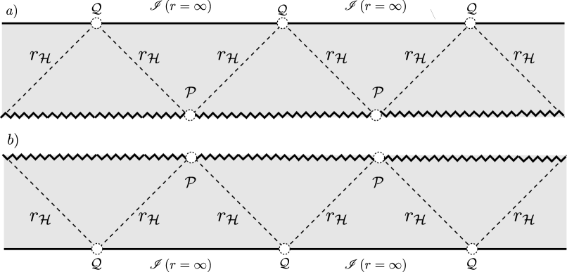
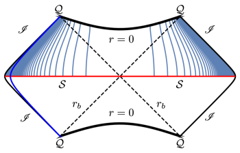
In this Section, for concreteness we restrict our discussion to the representation of the extremal Schwarzschild-de Sitter spacetime as a whitehole so that there the singularity lies in the past and the conformal boundary in the future —see Figure 2 (a).
Throughout this Section it is assumed that . In this case, vanishes at while for . Hence for , the coordinate is a time coordinate while is a spatial one. This means that the hypersurfaces with are spacelike while those of constant are timelike —see Figure 4. Consequently, one purports to construct a congruence of conformal geodesics by prescribing initial data on hypersurfaces of constant with and . In addition, observe that the critical curve located at as defined in Section 4.2.1 coincides in this case with the location of the Killing horizon .
5.1 Basic setup
Similar to the subextremal case we set
| (96) |
Hence and we get . This means that since is a constant along a given conformal geodesic. As in the case of Section 4, this choice simplifies the equations for the curve as these reduce to the equations of metric geodesics. In the remainder of this Section let
with a constant and —see Figure 7. As already pointed out, the above hypersurface of the extremal Schwarzschild-de Sitter spacetime is spacelike. Particularising equations (41) and (38) for the case we get
| (97) |
Remark 13.
Notice that in the extremal case and in contrast with the initial data chosen for the subextremal case the congruence is not necessarily orthogonal to the initial hypersurface . To see this more clearly, observe that the unit normal to is given by while . In particular, notice that and are not parallel and that . Compare this with the discussion for the subextremal Schwarzschild-de Sitter spacetime given in Section 4 where and the symmetry of the spacetime suggested to consider the initial hypersurface determined by the condition which has unit normal . In this case, setting leads to the initial data (51) for which and coincide —see Figure 4. In the extremal case however there is not a apriori preferred choice for determining the initial hypersurface —see Figure 7. Consequently, instead of prescribing data corresponding to a congruence starting orthogonal to we will consider as a free parameter so that, in general, the congruence can start oblique to the initial hypersurface.
Remark 14.
Observe that for the hypersurface is below the horizon while if then it lies above it. Our analysis will consider both situations simultaneously.
5.1.1 Conformal factor
Since one has that the 1-form vanishes. Using equation (22) and (24) one observes that . Taking into account equation (96) along with the constraints (20) one gets
For conciseness and consistency with the notation of Section 2 one sets . For the case of a de-Sitter like cosmological constant one sets . Moreover, without loss of generality let us set , then the conformal factor associated to the congruence defined by the initial data discussed in Section 5.1 is found by using the general expression (19)
where . The roots of are given by
| (98) |
Although one has formally two roots of the conformal factor , an inspection of the conformal diagram of Figure 7 reveals that only one component of the conformal boundary is actually realised. Moreover, in order to have finite, we restrict the possible values of to those that satisfy . This corresponds to restrict our analysis to compact conformal representations in which is located at a finite value of the unphysical proper time .
The relation between the unphysical proper time and the physical proper time is readily obtained form equation (21):
Therefore,
| (99) |
From these expressions we deduce that . For conciseness let us take so that and . Using equation (99) we see that the conformal factor can be rewritten in terms of the -proper time as
| (100) |
5.1.2 Initial conditions for the congruence
Unlike in the other cases studied in this article, we do not require the congruence to be everywhere orthogonal to the initial hypersurface . However, we are interested in showing that the curves arrive orthogonally to the conformal boundary. To do so we first compute
| (101) |
Observe that at . Hence, at . Now from (21) on has that
| (102) |
Using equation (41) one can consider , equivalently , therefore . Using the last observation and equations (101) and (102) and one gets
| (103) |
Recall now that, as described in Section 3.5, we are considering geodesic equations with no evolution in the angular coordinates, thus
since one is effectively analysing the curves on a 2-dimensional manifold with metric as given in equation (36). Therefore, one can define a unique orthogonal vector to by . A direct computation shows that
so that,
Hence, using (22) one has that
| (104) |
Therefore using equations (103), (104), (41) and (42) we get
Taking into account that and that
and then assuming one concludes
This means that the curves arrive orthogonally to the conformal boundary.
Remark 15.
A quick inspection of the last argument shows that one can perform a similar calculation for the congruence of conformal geodesics in the subextremal Schwarzschild-de Sitter spacetime of Section 4 and obtain the same conclusion.
Remark 16.
This is in agreement with Proposition 3.1 given in [7] where it is shown that in an Einstein spacetime, any conformal geodesic leaving orthogonally is up to reparametrisation a geodesic of .
5.2 Qualitative analysis of the behaviour of the curves
In this Section we carry out a qualitative study of the family of curves in the extremal Schwarzschild-de Sitter analogous to that of Section 4.2 for the subextremal case. We distinguish three basic types of curves: those escaping to the asymptotic points and those emanating from the singularity in the past and escaping to the conformal boundary in the future.
5.2.1 Conformal geodesics with constant
The condition determining the location of the curves with constant is given by
Since and given that only vanishes for positive at then, the critical curve is characterised by the conditions and . This is consistent with the analysis of Section 4.2.1 since as given in equation (59) reduces to for . Moreover, notice that by virtue of equation (42) and the initial data given in Section 5.1 conformal geodesics with and coincide with curves of constant . These curves accumulate at the asymptotic points and —see Figure 7. Observe that for and the expression (43a) can be explicitly integrated to yield
| (105) |
where
Observe that equation (105), as pointed out in [15], implies that the geodesics with never cross the horizon since as . Using equation (99) and setting for simplicity, we obtain
| (106) |
where .
Asymptotic behaviour of the curve. To analyse the behaviour of these curves as they approach the asymptotic points and let us consider . Then one obtains that for small that
where are numerical factor not relevant for the subsequent discussion. To leading order where we have used the value of and introduced and to simplify the notation. Consequently, to leading order we have
Since then one concludes that diverges as . Therefore the curves with become tangent to the Killing horizon as the approach the asymptotic points and . In other words, as in the subextremal case, these curves become asymptotically null.
5.2.2 Conformal geodesics with non-constant
Recalling that
and observing that , it follows that if then, in fact, . Moreover, one can show that and that for . Thus, the curves escape to the conformal boundary.
Behaviour towards the conformal boundary. We now show that the congruence of conformal geodesics reaches the conformal boundary in an infinite amount of physical proper time. In order to see this, first observe from equation (12) that , consequently from equation (41) it follows that is a monotonic function. Moreover, using equations (12) and (42) we find that
| (107) |
We are interested in analysing the convergence of
Introducing a new variable then we can rewrite the integral as
Since one has for some small. Thus . Therefore we have that
Using the latter, we have that
so that
This last integral diverges and one concludes that diverges as well. Accordingly, the conformal boundary is reached in an infinite amount of physical proper time.
Remark 17.
For initial hypersurfaces with (i.e. lying below the horizon), a direct inspection of the integral in
shows that it is finite —there are no zeros in the denominator for . Thus the horizon is reached in a finite amount of proper time.
Behaviour towards the singularity. We now shown that both the horizon and the singularity are reached by the curves of the congruence in a finite amount of physical proper time . This behaviour is a consequence of the fact that the integral in equation (107) is finite for any with . To prove this we start from the inequality
Therefore, for this entails
This last inequality shows the assertion. In what follows we denote by (respectively ) the value of the proper time at which the singularity is reached.
5.2.3 Behaviour of the congruence using null coordinates
Most of the analysis performed for the asymptotic region in the subextremal case in Section 4.2.2 can also be applied for the extremal case for any since in this case one has then the expression
is valid for any . This leads to formally the same estimates as in Section 4.2.2. Notice however that the congruence does not start orthogonally to the initial hypersurface . Assuming and performing formally the same procedure leading to equation (76) we get
| (108) |
This estimate is valid for any . In particular observe that is finite. Now, let us denote as before and take , then the same procedure leading to (77) renders
| (109) |
In contrast to Section 4.2.2, at this point one can compute the last integral using the explicit functional form for in the extremal case:
Observe that since one has that . Finally, using expressions (108), (109) and the triangle inequality render
| (110) |
Remark 18.
It follows then that the conformal geodesics cross the horizon and escape the conformal boundary with a finite value of the retarded null time . Thus, they remain away from the asymptotic points and .
Remark 19.
An analogous analysis can be carried out with the advanced null coordinate .
5.3 Explicit expressions in terms of elliptic functions
As in the subextremal case the solutions to the conformal geodesic equations can be written in terms of elliptic functions. We begin by observing that, using the functional form of as given in equation (12), one can rewrite
One can verify that the discriminant of the cubic is always negative provided that . Therefore one can factorise the above expression as
where while and are complex conjugate. Consequently, setting the integral (43a) can be written as
Curves with . Rather than considering the previous expression for an arbitrary non-vanishing value of the constant of integration , we now particularise to the case . This choice leads to simpler explicit expressions and can be done irrespectively of the value of . For a direct computation yields
| (111) |
where is an integration constant and one can verify that never vanishes. Thus, as given by the above expression is an analytic function of its arguments.
For the extremal Schwarzschild-de Sitter spacetime it is not possible to construct Kruskal-like coordinates. However, one can still construct null coordinates and using the tortoise radial coordinate . A straightforward computation shows that the tortoise coordinate in this case is given by
| (112) |
Observe that
Similarly, one can show that, taking the limit as approaches from the left () one has
| (113) |
while taking the limit from the right () one obtains
| (114) |
Taking into account expressions (111) and (112) and proceeding as in Section 4.2.4 one concludes that and are also analytic functions or their parameters. As previously discussed, in the extremal case the critical curve is characterised by the conditions and . Using equation (6) and the limits (113)-(114) one concludes that at the asymptotic points and one has respectively and .

5.4 Analysis of the conformal geodesic deviation equation
Given that for the initial data for the congruence we have set , it follows that the scalar describing the deviation of the congruence satisfies equation (94).
5.4.1 Initial data for the deviation equation
As previously discussed, one important difference between the extremal and the subextremal case is that in the former case is a time coordinate while is a spatial coordinate everywhere—thus, is a spatial vector. If the conformal geodesics end at the conformal boundary, while if the conformal geodesics end at the singularity. In the former case a suitable choice for the initial value of the deviation vector is . Proceeding in similar way as in Section 3.7 one gets and if one wants to analyse the behaviour of the congruence towards the conformal boundary. To analyse the behaviour towards the singularity it is convenient to set so that . In any case we can write which allow us to discuss both cases simultaneously.
5.4.2 Estimating the solution to the deviation equation
From equation (94), one readily obtains the estimate
Proceeding in an analogous way as in Section 4.4.2 we get
From the last expression it follows that for the case in which the conformal geodesics end at the singularity that so that there are no conjugate points in the congruence. In the case where the curves escape to the conformal boundary, one can proceed as follows: Using equation (100) one obtains
| (115) |
Notice that the expression on the right hand side of equation (115) is always finite, moreover
Therefore never vanishes not even at the conformal boundary.
5.5 Conformal Gaussian coordinates in the extremal Schwarzschild-de Sitter spacetime
In this Section we show how the congruence of conformal geodesics with can be used to construct a system of conformal Gaussian coordinates. In view of the periodicity of the maximal extension of the spacetime, the analysis will be restricted to the two triangles shown in Figure 7.
In what follows denote by eSdS the region in the conformal representation of the extremal Schwarzschild de Sitter spacetime defined by the conformal factor associated to the congruence of conformal geodesics given by Figure 7. On eSdS consider a spacelike hypersurface defined by the condition . For definiteness let so that the hypersurface is below the horizon. We use the restriction of the retarded null coordinate on to parametrise points on —in a slight abuse of notation we denote this restriction by ; observe that . Within eSdS we distinguish two subregions: lying towards the future of and lying towards the past.
The region . For and let and . In terms of these coordinates one has
The analysis in the previous Sections then shows that the map
with
as defined by the solutions to the conformal geodesic equations depends analytically on its parameters. Further the analysis of the conformal deviation equation shows that the Jacobian of the transformation is non-zero for the given range of parameters. Thus, it follows that the inverse map
with
is well defined and also an analytic function of its parameters. Thus, ignoring angular coordinates, this inverse map defines a conformal Gaussian system of coordinates in . In particular, given any point in , there is a unique conformal geodesic passing through it. Thus, the congruence of conformal geodesics covers the whole of .
The region . In terms of the coordinates , the region is described by
Again, the analysis carried out in the previous Sections shows that the map
is an analytic function of its parameters. Moreover, the analysis of the conformal geodesic deviation equation shows that it is invertible. Thus, the inverse map
is well-defined and an analytic function of its parameters. Thus, again ignoring angular coordinates, the inverse map defines a conformal Gaussian system of coordinates in . In particular, the congruence of conformal geodesics covers the whole of .
Remark 20.
Observe that the parallel horizons bounding the region eSdS are not covered by the congruence of timelike conformal geodesics.
5.6 Summary of the analysis
The analysis of the previous Sections can be summarised in the following proposition:
Proposition 1 (Conformal geodesics in the extremal Schwarzschild-de Sitter spacetime).
The portion of the extremal Schwarzschild-de Sitter spacetime corresponding to the region eSdS can be covered by a non-singular congruence of conformal geodesics emanating from the singularity at and escaping to the conformal boundary. This congruence can be used to construct a global system of conformal Gaussian coordinates in the spacetime.
6 The Schwarzschild-anti de Sitter spacetime
Consistent with the discussion of Section 2.1, for the Schwarzschild-anti de Sitter spacetime . The latter will be assumed throughout this Section. In this case one expects to be able to construct a congruence of conformal geodesics that combines the properties of congruences in the Schwarzschild and anti de Sitter spacetime.
6.1 Basic setup
In this Section we provide the initial data for the congruence of conformal geodesics in the Schwarzschild-anti de Sitter spacetime and analyse some of its basic properties.
6.1.1 Initial data
As in the case of the subextremal Schwarzschild-de Sitter solution, we set initial data for the congruence of conformal geodesics on the time symmetric hypersurface of the Schwarzschild-anti de Sitter spacetime. One requires the congruence to be orthogonal to , consequently, we set
| (116) |
where now is given by equation (13). To find a suitable initial conformal factor and the value of we first look at the limiting case . In this case the line element (3) reduces to
Using the the coordinate transformation the above line element of the anti de Sitter spacetime can be brought to the more standard form
It is well known the de Sitter spacetime is conformal to the static Einstein Universe . The conformal factor realising this conformal embedding is given by
| (117) |
To see this more clearly we introduce a coordinate via . Then a computation shows that is given by
Conformal geodesics for the anti-de Sitter spacetime have been studied in [4] —see also [17] for a discussion of conformal geodesics in the Minkowski, de-Sitter and anti de-Sitter spacetimes. Returning to the case, we will use the conformal factor given in equation (117) to fix the initial data for . A calculation readily gives that
The above 1-form suggests setting the initial data
| (118) |
so that
| (119) |
Notice that according to equation (40) the value of is fixed by the choice of initial data and it turns out to be
Hence, one has
Furthermore, using the constraints (20) one can readily compute the values of and . One has that
It follows from the above that
| (120) |
cannot vanish for any value of if . Accordingly, the conformal geodesics associated to this conformal factor do not intersect the conformal boundary unless they are initially tangent to it. Using the above conformal factor one can compute the the explicit relation between and using (21). One finds that
| (121) |
Remark 21.
Using formula (121) one can readily verify that for finite values of
Moreover, taking the double limit
This is a manifestation of a phenomenon already observed in the anti de Sitter spacetime in which the -proper time only covers a finite portion of the temporal extent of the Einstein cylinder —see [4]. In order to continue the description of a conformal geodesic with the -proper time one needs to perform a reparametrisation by means of a Möbius transformation —see e.g. [17].
6.1.2 Technical observations
With the choice of given by the positive square root of equation (118), the solution of equation (41) can be written as
| (122) |
where
Since , if are complex then . On the other hand, if are real then
Moreover, if are real, then we have the following result:
Lemma 3.
If and are real then
| (123) |
Proof.
One has the following explicit relations
We now notice that
| (124) |
which holds because as and all the factors are positive. Expanding out the product we find that the inequality (124) can be rewritten in the form
Under the assumptions that are real one has that , so that
| (125) |
Next use the identity
which enables us to write the inequality (125) in the form
Finally, as we conclude that . ∎
Lemma 4.
If then and .
Proof.
If then either
or
If are complex then and case (b) cannot hold so the lemma is proven. If are real then by virtue of Lemma 123 one has . If case (b) holds then which, in turn, can only be true if . Nevertheless, by Lemma 123, and, consequently, since then . However, this is a contradiction as . Therefore, case (b) cannot hold which then proves the lemma. ∎
Remark 22.
Notice that Lemma 4 implies that if the radicand in the right hand side of equation (122) is positive then necessarily . Consequently, is decreasing if . By continuity, is decreasing until it reaches a value of where vanishes. Using equation (41) one has that vanishes whenever vanishes. In other words, if are real then vanishes at where and at where . If are complex then is non-zero for so is always decreasing.
Remark 23.
In the sequel, to simplify the notation will be simply denoted by . Moreover, for future reference notice that equation (122) can be written as
| (126) |
Following the above discussion, depending on the sign of , we may distinguish three possibilities which are discussed.
6.2 Qualitative analysis of the behaviour of the curves
In this Section we analyse the different qualitative behaviours of the conformal geodesics defined by the initial conditions given in the previous Section. There are, broadly, three types of geodesics: a set of geodesics parallel to the conformal boundary, geodesics reaching timelike infinity and finally geodesics falling into the singularity.
6.2.1 Conformal geodesics entering the horizon
Consider such that . In this case are complex and is strictly positive. Therefore, there are no turning points and . The conformal geodesics get through the event horizon and end up in the singularity at
| (127) |
To verify that is finite observe that since is strictly positive then there exist a small such that . Consequently
Explicit expressions in terms of elliptic functions. In the case one has
One can use this information to rewrite the integral given in equation (126) in terms of elliptic functions. In particular, using formulae 259.07 and 361.62 of [2] with and parameters
one obtains
| (128) |
where , and denote the delta amplitude, the sine amplitude and cosine amplitude functions (Jacobi elliptic functions). The function is defined as and is the incomplete elliptic integral of the third kind. The constants and are determined in terms of and via
Remark 24.
The expression for given by (128) can be seen to be an analytic function of its arguments.
6.2.2 Critical conformal geodesic
We consider next such that . In this case has a double root and the integral expression (122) takes the form
with
In fact, in this particular case one can compute the integral in terms of elementary functions, the result being
| (129) |
where the integral is carried out using that and which arise respectively from Lemmas 123 and 4. Observe that
| (130) |
Hence we conclude that in equation (129) has to be taken such that .
Assumption 1.
For the subsequent discussion the location of relative to is required. Numerical evaluations suggest that . In the following will be assumed.
Notice that implies that this geodesic never enters into the black hole region. Hence the conformal geodesic starting at with satisfying the condition separates the conformal geodesics which go to the black hole region and end up in the singularity from those which do not enter this region. This conformal geodesic is depicted in Figure 9.
Remark 25.
It can be readily be verified that the expression for is an analytic expression of its parameters except at .
To further analyse the properties of the critical conformal geodesic we need to study the behaviour of as well. This analysis is carried out in the remainder of this Section. Using the chain rule and equations (41) and (42) we get
| (131) |
Replacing of , and for the Schwarzschild-anti de Sitter case, a computation renders
| (132) |
We use now the following inequalities
| (133) |
which are valid for all values of such that . From these we get
| (134) |
Hence
This shows that the critical conformal geodesic reaches infinite coordinate time but neither enters the black hole nor escapes to infinity. Therefore it asymptotes to a region which is neither conformal infinity nor the singularity.
6.2.3 Conformal geodesics not entering the horizon
Finally, consider values of for which . In this case the roots of the polynomial are real and Lemma 123 applies. This implies that and the limit
is finite. To see this, recall that equation (126) implies that the latter limit can be computed via
Fix a constant value with . Under these conditions we have the inequalities
from which
Hence,
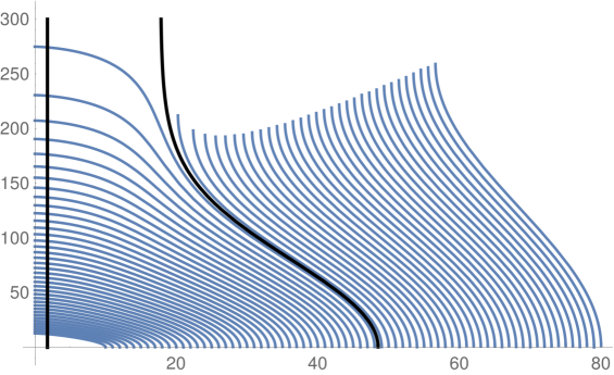
Thus, the value is reached in a finite amount of physical proper time. Now, it can be readily verified that at . Thus, at one has a turning point. The conformal geodesic reaching this point can be smoothly extended by means of a reflection of the conformal geodesic with respect to the horizontal line defined by . By repeating this procedure an infinite number of times one gets an inextendible curve which is a periodic function in the variable when represented in the form —see Figure 9. The period is given by . In particular, one has that, although the value of remains bounded for , it does not have a limit as . Moreover, making use of expression for the coordinate , one can readily verify that two consecutive turning points are reached in a finite amount of coordinate time . Also, an explicit computation shows that
which implies that the conformal geodesics approach a vertical line in the limit —the timelike conformal boundary.
Remark 26.
The late time behaviour of the conformal geodesics close to the conformal boundary in the Schwarzschild-de Sitter spacetime is similar to the behaviour observed in the anti de Sitter spacetime in which the vicinity of the conformal boundary (and, in fact, the whole spacetime) is ruled by conformal geodesics. Our analysis thus shows that there is an infinite number of conformal geodesics between the critical curve and the conformal boundary which neither fall into the black hole nor escape to the conformal boundary.
Explicit expressions in terms of elliptic functions. In the case one has three different subcases depending on the sign on :
All these cases can be discussed in a unified way using the formulae given in [2]. To do so, let
where denotes the sine amplitude function and is the incomplete elliptic integral of the first kind. For case a) using formula 257.02 of [2] with parameters
the integral (126) can be expressed as
For case b) using formula 257.13 of [2] with parameters
one obtains
For case c) using formula 257.15 of [2] with parameters
one obtains
In these expressions is the incomplete elliptic integral of the third kind.
6.2.4 Conformal geodesic starting at the bifurcation sphere
To study the conformal geodesic which starts at the bifurcation sphere it is necessary that we rewrite the conformal geodesic equations we have developed in Kruskal-like coordinates to cover the maximal extension of the Schwarzschild anti de Sitter spacetime.
To start the discussion notice that for the Schwarzschild-anti de Sitter solution, the Eddington-Finkelstein coordinates defined by equation (6) take the form
| (135a) | |||
| (135b) | |||
From these coordinates, one defines the usual Kruskal-like coordinates as follows:
where is a constant given by
The radial coordinate can be implicitly written in terms of the Kruskal-like coordinates by means of the relation
| (136) |
where
| (137) |
Using this relation, we can compute the explicit form of the metric in the Kruskal-like coordinates
| (138) | |||
A computation then shows that the conformal geodesic equations for curves with initial datum are given by
| (139a) | |||
| (139b) | |||
| (139c) | |||
with initial conditions
| (140a) | |||
| (140b) | |||
Equation (139c) entails
Combining the latter expression with the initial data for the congruence leads to
We can write equation (139a) as
from which one obtains
| (141) |
In this integral, the function is defined implicitly through the relation
| (142) |
obtained from equation (136) setting . Exploiting the last equation one makes a change of variables in the integral of equation (141) to obtain
| (143) |
where
The integral of equation (143) can be computed explicitly, and after lengthy algebra one obtains
One eliminates the variable in this equation using the previous formulae to get in terms of . This computation then renders
whose solution can be reduced to quadratures
The integral is convergent for any value of in the interval . In particular it enables us to compute the value of the physical time at which this conformal geodesic reaches the singularity:
| (144) |
Remark 27.
Summarising, the conformal geodesic starting at the bifurcation sphere reaches the singularity in a finite amount of (physical) proper time.
6.2.5 Conformal geodesics at the conformal boundary
An important property of the anti de Sitter spacetime is that the conformal boundary can be ruled by a congruence of conformal geodesics —see e.g. [4]. In this Section we show that the congruence of conformal geodesics in the Schwarzschild-anti de Sitter spacetime considered in the previous Sections extends to the conformal boundary to include curves with a similar property.
The approach to the construction of conformal geodesics followed in this article has been to solve the relevant equations in the physical spacetime —this strategy, however, cannot be followed to analyse conformal geodesics at the conformal boundary. In this case, one needs to formulate the conformal geodesic equations and their initial data in a conformal extension.
Start by considering the conformal factor chosen earlier in this Section —see equation (117)— and let
By introducing a new radial coordinate , the latter metric can be shown to extend smoothly to the conformal boundary defined by . In particular, the (Lorentzian) induced metric on (i.e. at ) is given by
the standard metric of —the 3-dimensional Einstein cylinder. On consider now the family of curves given by
| (145) |
These curves have tangent given by and can be readily shown to be geodesics of the metric . As is a (3-dimensional) Einstein space, then the curve given by equation (145) is, up to a reparametrisation, a conformal geodesic —see e.g. Lemma 5.2 in [17]. To find the reparametrisation exhibiting the conformal geodesic character of the curve one follows the argument of the proof of that Lemma and consider a candidate 1-form
The conformal geodesic equations (15a)-(15b) readily give that
where denotes differentiation with respect to . These equations can be solved to give
Now, a calculation readily yields . Accordingly, the conformal factor on satisfying the condition obeys the ordinary differential equation
This differential equation can be solved to give
so that, in particular, one has that
Using the conformal factor one obtains a different representative of the conformal class of conformal boundary of the spacetime —i.e. so that
where the parameter has been introduced as new time coordinate. This representative of the conformal class can be regarded as canonical as in it, the parameter is the proper time of the curve.
Summarising the previous discussion, we have found that the pair given by
| (146) |
are solutions to the -conformal geodesics. Observe that, in particular, as the curve and the 1-form are completely intrinsic to the conformal boundary, then where is the unit normal vector to the initial hypersurface.
Remark 28.
This result is, in fact, a general property of anti de Sitter-like spacetimes: a conformal geodesic in an anti-de Sitter-like spacetime which passes through a point , is tangent to at and which satisfies with the unit normal to and the so-called Friedrich scalar of the conformal representation, remains in and defines a conformal geodesic for the conformal structure of —see e.g. [17], Lemma 17.1. We recall that the Friedrich scalar at a timelike (or spacelike) conformal boundary is closely related to the extrinsic curvature of the hypersurface —in particular, if then the conformal boundary is extrinsically flat, see [17], Section 11.4.4. In this Section we show that the congruence of conformal geodesics for the Schwarzschild-anti de Sitter spacetime considered in the previous Sections can be extended to include curves on the conformal boundary with the above property.
Remark 29.
Relation between the conformal geodesics on the conformal boundary and those in the bulk. Finally, we analyse the relation between the family of curves on the conformal boundary of the Schwarzschild-anti de Sitter spacetime and the conformal geodesics in the interior of the spacetime that have been constructed earlier. To do this, it is recalled that the conformal geodesic equations (15a) and (15b) are conformally invariant under a rescaling if the 1-form transforms as
Thus, the initial data for the -conformal geodesic equations implied by the initial data for the -conformal geodesic equations in (118) satisfies
for all points in the conformal extension of the (physical) initial hypersurface . Moreover, it can be readily verified that the curves in (146) are orthogonal to . Thus, they are the limit of the family of conformal geodesics in the interior of the spacetime considered in this Section.
6.3 Analysis of the conformal geodesic deviation equation
In this Section we apply the formalism introduced in Section 3.4 to verify that the congruence of conformal geodesics in the Schwarzschild-anti de Sitter spacetime constructed in the previous Section is non-singular. Remarkably, the various classes of conformal geodesics in the Schwarzschild spacetime discussed in the previous Sections can be analysed simultaneously.
In the case of the Schwarzschild-anti de Sitter equation, equation (48) with the value of given by (118) takes the form
It is observed that since both and are positive, we have the inequality
Therefore, satisfies the differential inequality
The latter implies that the scalars and satisfy
where is the solution of
This differential equation can be explicitly solved, the result being
Thus, using that
Since the congruence never reaches the conformal boundary, one concludes that the congruence does not form caustic points.
Remark 30.
We stress that the previous analysis holds for the three types of conformal geodesics considered in the previous Section.
6.4 Conformal Gaussian coordinates in the Schwarzschild-anti de Sitter spacetime
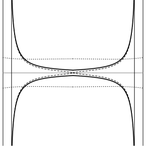
In Remark 21 it has been observed that the -proper time, , of the curves of the congruence of conformal geodesics in the Schwarzschild-anti de Sitter spacetime discussed in the previous Section does not cover the whole span of the curves. Thus, it follows that for the Schwarzschild-anti de Sitter spacetime it is not possible to construct global systems of conformal Gaussian coordinates as it was the case in the cases of positive and vanishing Cosmological constant.
Notwithstanding the observation made in the previous paragraph, under Assumption 1, and using methods similar to those employed in Sections 4.5 and 5.5 it is still possible to show that the congruence covers the maximal extension of the conformal representation of the spacetime defined by the conformal factor as given by equation (120). Taking advantage of the discrete symmetries of the spacetime, the discussion can be restricted to the range . We omit the details.
6.5 Summary
The analysis of Section 6 can be summarised in the following Theorem:
Theorem 2 (Conformal geodesics in the Schwarzschild-anti de Sitter spacetime).
A qualitatively accurate depiction of the congruence of conformal geodesics in the Penrose diagram for various values of the mass parameter is shown in Figures 10 and 11. A qualitatively accurate depiction of the region of the spacetime that can be covered by conformal Gaussian coordinates can be found Figure 12.
7 Concluding remarks
In this article we have studied conformal geodesics in the Schwarzschild -de Sitter and Schwarzschild-anti de Sitter families of spacetimes. In both cases, initial data for the congruence of curves can be chosen in such a manner that they cover the whole maximal extension of the spacetime. Moreover, in the case of the Schwarzschild-de Sitter spacetime, these curves provide global coordinate systems which, in turn, can be used as the starting point of a study of perturbations and global questions by means of conformal methods. To do this, one would need to study the exact solutions expressed in terms of the conformal Gaussian coordinates. As discussed in [8] for the Schwarzschild-de Sitter spacetime, this is not an easy task —in absence of an explicit change of coordinates one is forced to extract the required properties of the spacetime by means of a direct analysis of the evolution equations satisfied by the exact solution. In contrast in the Schwarzschild-anti de Sitter case only a portion of the maximal extension can be covered by conformal Gaussian coordinates. This phenomenon resembles the case of the anti de Sitter spacetime in which the conformal extension of the spacetime is only compact in the spatial directions but extends infinitely in the time direction. In this case, the unphysical proper time is exhausted before covering the full conformal extension of the spacetime.
Acknowledgements
AGP is supported by projects IT956-16 (Basque government, Spain), PTDC/MAT-ANA/1275/2014 (“Fundação para a Ciência e a Tecnología” (FCT), Portugal), FIS2014-57956-P (“Ministerio de Economía y Competitividad”, Spain) and EG holds a scholarship (494039/218141) from Consejo Nacional de Ciencia y Tecnología (CONACyT). AGP wishes to thank the School of Mathematical Sciences of Queen Mary College, where part of this work was carried out, for hospitality. The three authors thank Dr. Christian Lübbe for enlightening discussions.
References
- [1] S. L. Bażański & V. Ferrari, Analytic extension of the Schwarzschild-de Sitter metric, Nuovo Cimento B 91, 126 (1986).
- [2] P. Byrd & M. Friedman, Handbook of Elliptic Integrals for Engineers and Physicists, Grundlehren der mathematischen Wissenschaften, Springer Verlag, (2013).
- [3] L. Fidkowski, V. Hubeny, M. Kleban, & S. Shenker, The black hole singularity in AdS/CFT, J. High E. Phys. 2, 014 (2004).
- [4] H. Friedrich, Einstein equations and conformal structure: existence of anti-de Sitter-type space-times, J. Geom. Phys. 17, 125 (1995).
- [5] H. Friedrich, Conformal Einstein evolution, in The conformal structure of spacetime: Geometry, Analysis, Numerics, edited by J. Frauendiener & H. Friedrich, Lecture Notes in Physics, page 1, Springer, (2002).
- [6] H. Friedrich, Conformal geodesics on vacuum spacetimes, Comm. Math. Phys. 235, 513 (2003).
- [7] H. Friedrich & B. Schmidt, Conformal geodesics in general relativity, Proc. Roy. Soc. Lond. A 414, 171 (1987).
- [8] E. Gasperín & J. A. Valiente Kroon, Perturbations of the asymptotic region of the Schwarzschild-de Sitter spacetime, Ann. H. Poincaré (2017).
- [9] J. B. Griffiths & J. Podolský, Exact space-times in Einstein’s General Relativity, Cambridge University Press, (2009).
- [10] E. Hackmann & C. Lämmerzahl, Geodesic equation in Schwarzschild-(anti)-de Sitter spacetimes: analytical solutions and applications, Phys. Rev. D 78, 024035 (2008).
- [11] T. Klösch & T. Strobl, Classical and quantum gravity in dimensions. Part II: the universal coverings, Class. Quantum Grav. 13(2395) (1996).
- [12] D. F. Lawden, Elliptic functions and applications, Springer, (1989).
- [13] C. Lübbe & J. A. Valiente Kroon, On de Sitter-like and Minkowski-like spacetimes, Class. Quantum Grav. 26, 145012 (2009).
- [14] C. Lübbe & J. A. Valiente Kroon, A class of conformal curves in the Reissner-Nordström spacetime, Ann. Henri Poincaré 15, 1327 (2013).
- [15] J. Podolský, The structure of the extreme Schwarzschild-de Sitter spacetime, Gen. Rel. Grav. 31, 1703 (1999).
- [16] C. Stanciulescu, Spherically symmetric solutions of the vacuum Einstein field equations with positive cosmological constant, Master thesis, University of Vienna, (1998).
- [17] J. A. Valiente Kroon, Conformal Methods in General Relativity, Cambridge University Press, (2016).