Time-Dependent Perpendicular Transport of Energetic Particles in Magnetic Turbulence with Transverse Complexity

Abstract

The motion of energetic particles in magnetic turbulence across a mean magnetic field is explored analytically. The approach presented here allows for a full time-dependent description of the transport, including compound sub-diffusion. The first time it is shown systematically that as soon as there is transverse structure of the turbulence, diffusion is restored even if no Coulomb collisions are invoked. Criteria for sub-diffusion and normal Markovian diffusion are found as well.

One of the most fundamental problems in plasma physics and astrophysics is to understand the motion of energetic particles through a magnetized plasma. This motion is described by diffusion coefficients in the different directions of space. In particular the transport of particles across a large scale or guide magnetic field was subject of numerous analytical and numerical studies because of the complexity of this problem. Knowledge of diffusion parameters is important for a variety of applications such as space weather studies, acceleration of particles at shock waves, the propagation of cosmic rays through the universe, as well as the motion of fast particles in a fusion reactor (see Schlickeiser (2002); Wesson (2004); Balescu (2005) for reviews). The simplest model for perpendicular transport is based on the assumption that particles follow magnetic field lines while they move in the parallel direction with constant velocity. In this case the spread of particles across the mean magnetic field is entirely controlled by the stochasticity of magnetic field lines. Analytically this corresponds to the relation $\kappa_{\perp}=\kappa_{FL}v/2$ for the perpendicular diffusion coefficient (see Jokipii (1966)). Here we have used the particle speed $v$ and the field line diffusion coefficient $\kappa_{FL}$. Characteristic for this model is that the corresponding perpendicular mean free path $\lambda_{\perp}=3\kappa_{\perp}/v=3\kappa_{FL}/2$ does not depend on particle energy or momentum. In reality, however, one expects that pitch-angle scattering influences the particle orbit and, therefore, the assumption of an unperturbed motion is questionable. If strong pitch-angle scattering is present, perpendicular transport is suppressed to a sub-diffusive level. This type of transport is usually called compound sub-diffusion (see, e.g., Kóta & Jokipii (2000); Webb et al. (2006)). Characteristic for this type of transport is that the mean square displacement (MSD) of possible particle trajectories scales like $\langle(\Delta x)^{2}\rangle\propto\sqrt{t}$ with time. Therefore, normal Markovian diffusion, where we would have by definition $\langle(\Delta x)^{2}\rangle\propto t$, cannot be found. Thus, the question arises what physical effect is required in order to restore normal diffusion. According to the famous work of Rechester & Rosenbluth (see Rechester & Rosenbluth (1978)), Coulomb collisions can recover diffusion but cases have been found in which lacking collisions entirely, perpendicular transport is still diffusive (see, e.g., Giacalone & Jokipii (1999); Qin et al. (2002)). In such numerical work evidence is provided that transverse complexity of the turbulence alone can restore Markovian diffusion, at least in the late time limit. Obviously perpendicular transport is a complex non-linear process and, therefore, it is challenging to develop analytical theories for this type of transport (see, e.g., Rechester & Rosenbluth (1978); Krommes et al. (1983); Bieber & Matthaeus (1997); Matthaeus et al. (2003); Shalchi et al. (2004)). The unified non-linear transport (UNLT, Shalchi (2010)) theory agrees with performed test-particle simulations for a variety of magnetic field configurations including turbulence with small and large Kubo numbers as well as two-component turbulence (see, e.g., Tautz & Shalchi (2011); Shalchi & Hussein (2014)). However, such previous theories rely on the assumption of diffusive perpendicular transport. Therefore, the following questions remain unanswered:

1. What exactly triggers perpendicular diffusion if there are no Coulomb collisions and what are the effects and times scales leading to Markovian diffusion?

2. Can we develop a time-dependent theory of perpendicular transport which can describe compound sub-diffusion at early times and then the restoration of diffusion for later times?

In the current letter we develop a time-dependent non-linear theory for perpendicular transport in order to answer the those questions.

The fundamental equation describing the motion of charged particles through purely magnetic turbulence is the Newton-Lorentz equation $d\vec{p}/dt=q\vec{v}\times\vec{B}(\vec{x})/c$ where the total magnetic field is given as superposition of a mean or guide field and a turbulent component, i.e. $\vec{B}(\vec{x})=\delta\vec{B}(\vec{x})+B_{0}\vec{e}_{z}$. Furthermore, we have used the electric charge of the energetic particle $q$, the particle velocity $\vec{v}$, the particle momentum $\vec{p}$, as well as the speed of light $c$. If the particle position $\vec{x}$ is replaced by guiding center coordinates $\vec{X}=\vec{x}+(\vec{v}\times\vec{e}_{z})/\Omega$ (see, e.g., Schlickeiser (2002)), the Newton-Lorentz equation provides the following equations of motion

$$V_{x}=v_{z}\frac{\delta B_{x}\left(\vec{x}\right)}{B_{0}}\quad\textnormal{and}\quad V_{y}=v_{z}\frac{\delta B_{y}\left(\vec{x}\right)}{B_{0}}$$ (1)

where $V_{x}$ and $V_{y}$ are the perpendicular components of the guiding center velocity. The gyrofrequency is given by $\Omega=(qB_{0})/(mc\gamma)$ with the rest mass of the particle $m$ and the Lorentz factor $\gamma$. In the following we assume that the diffusion coefficients based on particle and guiding center coordinates are the same. In analytical descriptions of turbulence, the magnetic field in Eq. (1) is replaced by a Fourier representation. Problematic in Eq. (1) is the parallel component of the particle velocity $v_{z}$ because there is no simple way of modeling this quantity due to the chaotic nature of the particle motion. Furthermore, it was shown that particle velocity and position are strongly correlated (see, e.g., Shalchi (2010)). Based on Shalchi (2005) we write

$$V_{x}(t)=\frac{1}{B_{0}}\int d^{3}k\;\delta B_{x}\left(\vec{k}\right)\frac{1}{ik_{\parallel}}\left(\frac{d}{dt}e^{izk_{\parallel}}\right)e^{i\vec{x}_{\perp}\cdot\vec{k}_{\perp}}.$$ (2)

A similar equation can be obtained for $V_{y}$. However, due to the assumption of axi-symmetric turbulence, this would lead to the same result for the diffusion coefficient. Perpendicular transport is described by the auto-correlation function $\langle V_{x}(t)V_{x}(0)\rangle$ where the guiding center velocity is given by Eq. (2). In the following we assume that the magnetic fields and the phases in Eq. (2) are uncorrelated. In the literature this type of approximation is either called random phase approximation or Corrsin’s independence hypothesis (see Corrsin (1959)). This type of approximation could be inaccurate in real magnetic turbulence which is spatially intermittent (see, e.g., Burlaga & Vinas (2004)). Furthermore, we assume that the turbulence is homogeneous $\langle\delta B_{x}(\vec{k})\delta B_{x}^{*}(\vec{k}^{\prime})\rangle=\delta(\vec{k}-\vec{k}^{\prime})P_{xx}(\vec{k})$ where we have used the Dirac delta and the $xx$-component of the magnetic correlation tensor. As an additional assumption we employ the hypothesis $\langle\exp{[i\vec{x}\cdot\vec{k}]}\rangle\approx\langle\exp{[izk_{\parallel}]}\rangle\langle\exp{[i\vec{x}_{\perp}\cdot\vec{k}_{\perp}]}\rangle$. Therefore, we can write the auto-correlation function as

$$\langle V_{x}(t)V_{x}(0)\rangle=\frac{1}{B_{0}^{2}}\int d^{3}k\;P_{xx}\left(\vec{k}\right)\xi\left(t,0\right)\left<e^{i\vec{x}_{\perp}\cdot\vec{k}_{\perp}}\right>$$ (3)

where we have used the parallel correlation function

$$\xi\left(t_{1},t_{2}\right)=k_{\parallel}^{-2}\left<\left(\frac{d}{dt_{1}}e^{iz(t_{1})k_{\parallel}}\right)\left(\frac{d}{dt_{2}}e^{-iz(t_{2})k_{\parallel}}\right)\right>$$ (4)

and assumed that $\vec{x}_{\perp}(t=0)=0$. The parallel correlation function (4) can be integrated over times $t_{1}$ and $t_{2}$. Thereafter we calculate the derivatives with respect to $t_{1}$ and $t_{2}$. With $z(0)=0$ this trick allows us to write

$$\xi\left(t_{1},t_{2}\right)=k_{\parallel}^{-2}\frac{d}{dt_{1}}\frac{d}{dt_{2}}\left<e^{i\left[z\left(t_{1}\right)-z\left(t_{2}\right)\right]k_{\parallel}}\right>.$$ (5)

In order to compute a time-dependent diffusion coefficient $d_{\perp}(t)=d\langle(\Delta x)^{2}\rangle/(2dt)$, we employ the TGK (Taylor-Green-Kubo) formulation (see Taylor (1922); Green (1951); Kubo (1957))

$$d_{\perp}(t)=d_{\perp}(0)+\Re\int_{0}^{t}dt^{\prime}\;\left<V_{x}(t^{\prime})V_{x}(0)\right>$$ (6)

where we allow a non-vanishing initial diffusion coefficient. For the perpendicular characteristic function in Eq. (3) we employ $\langle\exp{[i\vec{x}_{\perp}\cdot\vec{k}_{\perp}]}\rangle=\exp{[-\langle(\Delta x)^{2}\rangle k_{\perp}^{2}/2]}$ corresponding to a Gaussian distribution with vanishing mean. Furthermore, we can use Eqs. (3) and (6) to write

$$\frac{d^{2}}{dt^{2}}\langle(\Delta x)^{2}\rangle=\frac{2}{B_{0}^{2}}\int d^{3}k\;P_{xx}\left(\vec{k}\right)\xi\left(t,0\right)e^{-\frac{1}{2}\langle(\Delta x)^{2}\rangle k_{\perp}^{2}}.$$ (7)

This ordinary differential equation can be evaluated for any given turbulence model described by the magnetic correlation tensor $P_{nm}$ as long as the parallel correlation function $\xi(t_{1},t_{2})$ is specified as well. It has to be emphasized that at not point we have assumed that perpendicular transport is diffusive. In the following we combine Eq. (7) with a diffusion approximation and consider the case of weak and strong pitch-angle scattering, respectively. Thereafter, we demonstrate how Eq. (7) explains compound sub-diffusion and the recovery of diffusion for turbulence with transverse structure.

If pitch-angle scattering is suppressed we can set $z(t)=v\mu t$ in Eq. (5). Here we have used the constant pitch-angle cosine $\mu$. For the perpendicular MSD we employ the diffusion approximation $\langle(\Delta x)^{2}\rangle=2D_{\perp}t$ where we have used the pitch-angle dependent Fokker-Planck coefficient $D_{\perp}(\mu)$. Therewith, Eq. (7) becomes

$$\langle V_{x}(t)V_{x}(0)\rangle=\frac{v^{2}\mu^{2}}{B_{0}^{2}}\int d^{3}k\;P_{xx}\left(\vec{k}\right)e^{iv\mu tk_{\parallel}-D_{\perp}k_{\perp}^{2}t}.$$ (8)

Using Eq. (6) with $d_{\perp}(0)=0$, and integrating Eq. (8) over time gives

$$D_{\perp}=\frac{v^{2}\mu^{2}}{B_{0}^{2}}\int d^{3}k\;P_{xx}\left(\vec{k}\right)\frac{D_{\perp}k_{\perp}^{2}}{\left(D_{\perp}k_{\perp}^{2}\right)^{2}+\left(v\mu k_{\parallel}\right)^{2}}.$$ (9)

We can easily see that $D_{\perp}\propto|\mu|$. Therefore, we can write the solution as $D_{\perp}=2\left|\mu\right|\kappa_{\perp}$ so that $\kappa_{\perp}=\frac{1}{2}\int_{-1}^{+1}d\mu\;D_{\perp}(\mu)$ (see, e.g., Schlickeiser (2002)). Thus, Eq. (9) becomes

$$\kappa_{\perp}=\frac{v^{2}}{3B_{0}^{2}}\int d^{3}k\;\frac{P_{xx}(\vec{k})}{F(\vec{k})+4\kappa_{\perp}k_{\perp}^{2}/3}$$ (10)

with the function

$$F(k_{\parallel},k_{\perp})=(vk_{\parallel})^{2}/(3\kappa_{\perp}k_{\perp}^{2}).$$ (11)

Eq. (10) can be written as $\kappa_{\perp}=v\kappa_{FL}/2$ where $\kappa_{FL}$ is the field line diffusion coefficient. Combined with this form, Eq. (10) becomes equivalent to the integral equation for field line diffusion derived in Matthaeus et al. (1995). The solution found here is called the field line random walk limit. Eqs. (9) and (10) also contain quasi-linear theory originally derived in Jokipii (1966). The latter theory can be obtained by employing the limiting processes $D_{\perp}\rightarrow 0$ or $\kappa_{\perp}\rightarrow 0$, respectively. In the opposite case one can find the result of Kadomtsev & Pogutse (see Kadomtsev & Pogutse (1978)) as shown in Shalchi (2015).

In astrophysics pitch-angle scattering is usually strong. Therefore, we now assume that parallel transport becomes diffusive instantaneously and employ the characteristic function of a diffusion equation $\langle\exp{[i\left(z(t_{1})-z(t_{2})\right)k_{\parallel}]}\rangle=\exp{[-\kappa_{\parallel}k_{\parallel}^{2}|t_{1}-t_{2}|]}$. Therewith, we derive from Eq. (5)

$$\xi\left(t_{1},t_{2}\right)=-\kappa_{\parallel}^{2}k_{\parallel}^{2}e^{-\kappa_{\parallel}k_{\parallel}^{2}\left|t_{1}-t_{2}\right|}.$$ (12)

With the latter formula and the diffusion approximation $\langle(\Delta x)^{2}\rangle=2\kappa_{\perp}t$, Eq. (7) becomes

$$\langle V_{x}(t)V_{x}(0)\rangle=-\frac{\kappa_{\parallel}^{2}}{B_{0}^{2}}\int d^{3}k\;P_{xx}(\vec{k})k_{\parallel}^{2}e^{-\kappa_{\parallel}k_{\parallel}^{2}t-\kappa_{\perp}k_{\perp}^{2}t}.$$ (13)

The next step is the application of the TGK formula (6). Here we have to be careful because the running diffusion coefficient at initial time is not zero due to the assumption of instantaneous parallel diffusion. Thus, we employ $d_{\perp}(t=0)=\kappa_{\parallel}\delta B_{x}^{2}/B_{0}^{2}$ where we have used $\delta B_{x}^{2}=\int d^{3}k\;P_{xx}(\vec{k})$. This corresponds to the assumption of instantaneous parallel diffusion and the interaction with ballistic magnetic field lines (see e.g., Zybin & Istomin (1985); Shalchi (2008)). With $\kappa_{\perp}=d_{\perp}(t=\infty)$ we derive from Eq. (13)

$$\kappa_{\perp}=\frac{v^{2}}{3B_{0}^{2}}\int d^{3}k\;\frac{P_{xx}(\vec{k})}{F(\vec{k})+v/\lambda_{\parallel}}$$ (14)

with the parallel mean free path $\lambda_{\parallel}=3\kappa_{\parallel}/v$ and the function $F(k_{\parallel},k_{\perp})$ defined in Eq. (11). As demonstrated in Shalchi (2015), Eq. (14) provides the same scaling as obtained in the famous work of Rechester & Rosenbluth if small Kubo number turbulence is considered. For the opposite case the Zybin & Istomin scaling (see Zybin & Istomin (1985)) is obtained.

Eqs. (10) and (14) are very similar. In order to find an integral equation covering both cases, we make the Ansatz

$$\kappa_{\perp}=\frac{v^{2}}{3B_{0}^{2}}\int d^{3}k\;\frac{P_{xx}(\vec{k})}{F(\vec{k})+(4/3)\kappa_{\perp}k_{\perp}^{2}+v/\lambda_{\parallel}}.$$ (15)

In the formal limit $\lambda_{\parallel}\rightarrow\infty$ we recover Eq. (10) and for $\lambda_{\parallel}\rightarrow 0$, on the other hand, we find Eq. (14). Therefore, Eq. (15) correctly describes both cases, strong and weak pitch-angle scattering. Eq. (15) is in perfect agreement with the integral equation provided by UNLT theory. In Shalchi (2010) this theory was derived by employing lengthy calculations based on the pitch-angle dependent Fokker-Planck equation. In the current paper we found an alternative but also a more intuitive derivation of UNLT theory.

In the following we drop the assumption of diffusive perpendicular transport but specify the properties of the magnetic fields. As a first example we employ the slab model $P_{nm}(\vec{k})=g(k_{\parallel})\delta(k_{\perp})\delta_{nm}/k_{\perp}$ where we have used the one-dimensional spectrum $g(k_{\parallel})$. For instantaneous parallel diffusion Eq. (3) becomes

$$\langle V_{x}(t)V_{x}(0)\rangle=-4\pi\frac{\kappa_{\parallel}^{2}}{B_{0}^{2}}\int_{0}^{\infty}dk_{\parallel}\;g\left(k_{\parallel}\right)k_{\parallel}^{2}e^{-\kappa_{\parallel}k_{\parallel}^{2}t}$$ (16)

and from Eq. (6) we derive for the running diffusion coefficient

$$d_{\perp}(t)=4\pi\frac{\kappa_{\parallel}}{B_{0}^{2}}\int_{0}^{\infty}dk_{\parallel}\;g\left(k_{\parallel}\right)e^{-\kappa_{\parallel}k_{\parallel}^{2}t}.$$ (17)

In the limit $t\rightarrow\infty$ we can approximate

$$d_{\perp}(t)\approx\frac{4\pi\kappa_{\parallel}}{B_{0}^{2}}g\left(k_{\parallel}=0\right)\int_{0}^{\infty}dk_{\parallel}\;e^{-\kappa_{\parallel}k_{\parallel}^{2}t}.$$ (18)

For the turbulence spectrum $g(k_{\parallel})$ we employ the Bieber et al. (see Bieber et al. (1994)) model

$$g(k_{\parallel})=\frac{1}{2\pi}C(s)\delta B^{2}l_{\parallel}\left[1+(k_{\parallel}l_{\parallel})^{2}\right]^{-s/2}$$ (19)

with $C(s)=\Gamma(s/2)[2\sqrt{\pi}\Gamma((s-1)/2)]$ where we have used the inertial range spectral index $s$ and gamma functions. The parameter $l_{\parallel}$ is the correlation length in the parallel direction. Therewith, we derive from Eq. (18)

$$d_{\perp}(t)=C(s)l_{\parallel}\frac{\delta B^{2}}{B_{0}^{2}}\sqrt{\frac{\pi\kappa_{\parallel}}{t}}$$ (20)

corresponding to compound sub-diffusion as described before in Kóta & Jokipii (2000); Webb et al. (2006).

In order to restore diffusion in the collisionless case, we need transverse structure. Although more complex anisotropic models for magnetohydrodynamic turbulence have been discussed in the literature (see, e.g., Goldreich & Sridhar (1995); Chandran (2000); Yan & Lazarian (2002); Boldyrev (2006)), we employ a simple noisy slab model defined via

$$P_{mn}(\vec{k})=\frac{2l_{\perp}}{k_{\perp}}g(k_{\parallel})\Theta\left(1-k_{\perp}l_{\perp}\right)\left(\delta_{mn}-\frac{k_{m}k_{n}}{k_{\perp}^{2}}\right)$$ (21)

where we have used the Heaviside step function $\Theta(x)$ and the perpendicular correlation length of the turbulence $l_{\perp}$. This model can be understood as broadened slab turbulence. If we assume again instantaneous parallel diffusion, we can combine Eqs. (7), (12), and (21). The perpendicular wavenumber integral therein can be expressed by an error function and we derive

$$\frac{d^{2}}{dt^{2}}\langle(\Delta x)^{2}\rangle = -8\pi\frac{\kappa_{\parallel}^{2}}{B_{0}^{2}}l_{\perp}\sqrt{\frac{\pi}{2\langle(\Delta x)^{2}\rangle}}\textnormal{Erf}\left(\sqrt{\frac{\langle(\Delta x)^{2}\rangle}{2l_{\perp}^{2}}}\right)$$ (22)

$$\times \int_{0}^{\infty}dk_{\parallel}\;g\left(k_{\parallel}\right)k_{\parallel}^{2}e^{-\kappa_{\parallel}k_{\parallel}^{2}t}.$$

One can easily demonstrate that for $\langle(\Delta x)^{2}\rangle\ll 2l_{\perp}^{2}$ one recovers Eq. (16) and we find the sub-diffusive result discussed above. In order to find new physics, we need to satisfy the condition $\langle(\Delta x)^{2}\rangle\gg 2l_{\perp}^{2}$. For a numerical evaluation of Eq. (22), it is convenient to employ the integral transformation $x=l_{\parallel}k_{\parallel}$ and to use the Kubo number $K=(l_{\parallel}\delta B_{x})/(l_{\perp}B_{0})$, the dimensionless time $\tau=\kappa_{\parallel}t/l_{\parallel}^{2}$, as well as $\sigma=\langle(\Delta x)^{2}\rangle/l_{\perp}^{2}$. With Eq. (19) for the spectrum $g(k_{\parallel})$, we deduce

$$\frac{d^{2}}{d\tau^{2}}\sigma = -4\sqrt{\pi}C(s)K^{2}\sqrt{\frac{2}{\sigma}}\;\textnormal{Erf}\left(\sqrt{\frac{\sigma}{2}}\right)$$ (23)

$$\times \int_{0}^{\infty}dx\;x^{2}\left(1+x^{2}\right)^{-s/2}e^{-\tau x^{2}}.$$

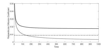
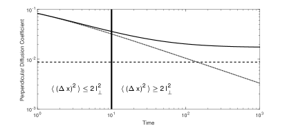
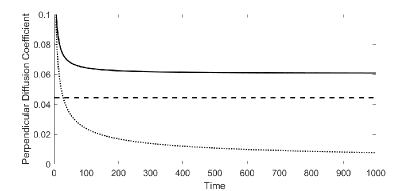
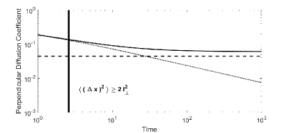
The latter differential equation can be solved numerically. The corresponding running diffusion coefficient $D_{\perp}=(l_{\perp}^{2}d_{\perp})/(l_{\parallel}^{2}\kappa_{\parallel})$ is shown in Fig. 1 for a Kubo number of $K=0.5$ and in Fig. 2 for a Kubo number of $K=0.75$, respectively. We also show the collisionless Rechester & Rosenbluth (CLRR) limit

$$\frac{\kappa_{\perp}}{\kappa_{\parallel}}=\left[\frac{\pi}{2}C(s)\frac{l_{\parallel}}{l_{\perp}}\frac{\delta B^{2}}{B_{0}^{2}}\right]^{2}$$ (24)

which can be derived from UNLT theory for small Kubo numbers and short parallel mean free paths (see Shalchi (2015)). According to Figs. 1 and 2, we find compound sub-diffusion for early times. As soon as the condition $\langle(\Delta x)^{2}\rangle\gg 2l_{\perp}^{2}$ is satisfied, normal Markovian diffusion is recovered due to the transverse structure of the turbulence. The final diffusion coefficient is close to the CLRR limit.

Figure 1: The running diffusion coefficient $D_{\perp}$ versus time $\tau$ as obtained by solving Eq. (23) numerically for a Kubo number of $K=0.5$ (solid lines). The dotted lines describe compound sub-diffusion as obtained from Eq. (20) and the dashed lines the (diffusive) CLRR limit represented by Eq. (24). In the lower panel the graphs are shown as double-logarithmic plot to emphasize the turnover from the sub-diffusive to the normal diffusive regime.

Figure 2: As in Fig. 1, but here we have considered a Kubo number of $K=0.75$.

In the current article we presented a detailed analytical study of perpendicular transport. The first time we have shown analytically that perpendicular transport is diffusive even if there are no Coulomb collisions invoked. Perpendicular diffusion is restored entirely due to transverse complexity of the turbulence. For turbulence without any transverse structure we find the usual sub-diffusive behavior. As soon as the condition $\langle(\Delta x)^{2}\rangle\gg 2l_{\perp}^{2}$ is satisfied, Markovian diffusion is recovered (see Figs. 1 and 2). In combination with a diffusion approximation, we found an alternative derivation of UNLT theory which showed good agreement with test-particle simulations performed in the past. The original derivation of UNLT theory relies on lengthy calculations based on the cosmic ray Fokker-Planck equation. The alternative derivation presented here, is shorter and more intuitive. The fact that the same integral equation (see, e.g., Eq. (15) of the current paper) is obtained confirms the validity of UNLT theory. Eq. (7) allows for a full time-dependent description of perpendicular transport. Especially in small Kubo number turbulence, particles can move sub-diffusively for a long time before reaching the diffusive regime. There will be several applications of the time-dependent description in a variety of physical scenarios ranging from fast particles is fusion reactors to cosmic rays in the solar system, the interstellar medium, and other astrophysical systems.

Support by the Natural Sciences and Engineering Research Council of Canada (NSERC) is acknowledged.

References

- Schlickeiser (2002) R. Schlickeiser, Cosmic Ray Astrophysics (Springer-Verlag, Berlin, 2002).
- Wesson (2004) J. Wesson, Tokamaks (Clarendon, Oxford, 2004).
- Balescu (2005) R. Balescu, Aspects of Anomalous Transport in Plasmas (Institute of Physics Publishing, Bristol, 2005).
- Jokipii (1966) J.R. Jokipii, Astrophy. J. 146, 480 (1966).
- Kóta & Jokipii (2000) J. Kóta and J.R. Jokipii, Astrophys. J. 531, 1067 (2000).
- Webb et al. (2006) G.M. Webb, G.P. Zank, E.Kh. Kaghashvili, and J.A. le Roux, Astrophys. J. 651, 211 (2006).
- Rechester & Rosenbluth (1978) A.B. Rechester and M.N. Rosenbluth, Phys. Rev. Lett. 40, 38 (1978).
- Giacalone & Jokipii (1999) J. Giacalone and J.R. Jokipii, Astrophys. J. 520, 204 (1999).
- Qin et al. (2002) G. Qin, W.H. Matthaeus, and J.W. Bieber, Astrophys. J. 578, L117 (2002).
- Krommes et al. (1983) J.A. Krommes, C. Oberman, and R.G. Kleva, J. Plasma Phys. 30, 11 (1983).
- Bieber & Matthaeus (1997) J.W. Bieber and W.H. Matthaeus, Astrophys. J. 485, 655 (1997).
- Matthaeus et al. (2003) W.H. Matthaeus, G. Qin, J.W. Bieber, and G.P. Zank, Astrophys. J. 590, L53 (2003).
- Shalchi et al. (2004) A. Shalchi, J.W. Bieber, W.H. Matthaeus, and G. Qin, Astrophys. J. 616, 617 (2004).
- Shalchi (2010) A. Shalchi, Astrophys. J. 720, L127 (2010).
- Tautz & Shalchi (2011) R.C. Tautz and A. Shalchi, Astrophys. J. 735, 92 (2011).
- Shalchi & Hussein (2014) A. Shalchi and M. Hussein, Astrophys. J. 794, 56 (2014).
- Shalchi (2005) A. Shalchi, J. Geophys. Res. 110, A09103 (2005).
- Corrsin (1959) S. Corrsin, Advances in Geophysics 6, 141 (1959).
- Burlaga & Vinas (2004) L.F. Burlaga and A. Vinas, J. Geophys. Res. 109, A12107 (2004).
- Taylor (1922) G.I. Taylor, Proceedings of the London Mathematical Society 20, 196 (1922).
- Green (1951) M.S. Green, J. Chem. Phys. 19, 1036 (1951).
- Kubo (1957) R. Kubo, J. Phys. Soc. Jpn. 12, 570 (1957).
- Matthaeus et al. (1995) W.H. Matthaeus, P.C. Gray, D.H. Pontius Jr., and J.W. Bieber, Phys. Rev. Lett. 75, 2136 (1995).
- Kadomtsev & Pogutse (1978) B.B. Kadomtsev and O.P. Pogutse, Plasma Phys. Controlled Nucl. Fusion Res. 40, 38 (1978).
- Shalchi (2015) A. Shalchi, Phys. Plasmas 22, 010704 (2015).
- Zybin & Istomin (1985) K.P. Zybin and Y.N. Istomin, Zh. Eksp. Teor. Fiz. 89, 836 (1985).
- Shalchi (2008) A. Shalchi, PP & CF 50, 055001 (2008).
- Bieber et al. (1994) J.W. Bieber ,W.H. Matthaeus, C.W. Smith, W. Wanner, M.-B. Kallenrode, and G. Wibberenz, Astrophys. J. 420, 294 (1994).
- Goldreich & Sridhar (1995) P. Goldreich and S. Sridhar, Astrophys. J. 438, 763 (1995).
- Chandran (2000) B.D.G. Chandran, Phys. Rev. Lett. 85, 4656 (2000).
- Yan & Lazarian (2002) H. Yan and A. Lazarian, Phys. Rev. Lett. 89, 281102 (2002).
- Boldyrev (2006) S. Boldyrev, Phys. Rev. Lett. 96, 115002 (2006).