Groundstate fidelity phase diagram of the fully anisotropic two-leg spin-${\textstyle\frac{1}{2}}$ $XXZ$ ladder

Abstract

The fully anisotropic two-leg spin-${\textstyle\frac{1}{2}}$ $XXZ$ ladder model is studied in terms of an algorithm based on the tensor network representation of quantum many-body states as an adaptation of projected entangled pair states to the geometry of translationally invariant infinite-size quantum spin ladders. The tensor network algorithm provides an effective method to generate the groundstate wave function, which allows computation of the groundstate fidelity per lattice site, a universal marker to detect phase transitions in quantum many-body systems. The groundstate fidelity is used in conjunction with local order and string order parameters to systematically map out the groundstate phase diagram of the ladder model. The phase diagram exhibits a rich diversity of quantum phases. These are the ferromagnetic, stripe ferromagnetic, rung singlet, rung triplet, Néel, stripe Néel and Haldane phases, along with the two $XY$ phases $XY1$ and $XY2$.

Keywords: $XXZ$ spin ladder, quantum phases, quantum fidelity, tensor networks

1 Introduction

Spin ladder systems have attracted considerable attention from both experimentalists and theoreticians alike [1, 2]. One of the most striking features of the simple spin-${\textstyle\frac{1}{2}}$ Heisenberg ladder is that the spin excitations are gapful (gapless) when the number of legs is even (odd) [3]. Spin ladder systems in general represent a particularly interesting class of quantum critical phenomena, exhibiting a rich variety of quantum phases [4, 5, 6, 7, 8]. Apart from a few cases [2], spin ladder systems are not exactly solvable, therefore it is necessary to develop various techniques, both analytical and numerical, to investigate their physical properties [9, 10, 11, 12, 13, 14, 15, 16, 17, 18, 19].

An efficient tensor network (TN) algorithm has been developed which is tailored to translationally invariant infinite-size spin ladder systems [20]. The algorithm is based on an adaptation to the ladder geometry of projected entangled pair states [21], a representation of quantum many-body wave functions. The spin ladder TN algorithm has been successfully applied to a variety of models [20, 22], including the ferromagnetic frustrated two-leg ladder, the two-leg Heisenberg spin ladder with cyclic four-spin exchange and cross couplings, and the three-leg Heisenberg spin ladder with staggering dimerization. The algorithm is seen to be efficient compared to the density matrix renormalization group [12] and time evolving block decimation [23], at least as far as the memory cost is concerned.

The TN representation offers an efficient way to detect quantum phase transitions in many-body quantum systems [24, 25] using the groundstate fidelity per lattice site [26, 27, 29, 28, 30, 31] (for other work on the fidelity approach to quantum phase transitions, see also [32, 33, 34, 35]). We recall that fidelity, as a measure of quantum state distinguishability in quantum information science, describes the distance between two given quantum states. It offers a powerful means to investigate critical phenomena in quantum many-body lattice systems, as demonstrated in Refs. [26, 27, 29, 28, 30, 31]. For example, the groundstate fidelity per lattice site enables the characterization of drastic changes of the groundstate wave functions in the vicinity of a phase transition point. A systematic scheme to study critical phenomena in quantum many-body lattice systems has been outlined using this approach [36]. Once the groundstate phase diagram is mapped out by means of the groundstate fidelity per lattice site, the local order parameters can be derived from the reduced density matrices for a representative groundstate wave function in a symmetry-broken phase. Other phases without any long-range order can also be detected and further characterized by nontrival order parameters such as string order and pseudo-order parameters.

In this paper we use the TN algorithm developed in Ref. [20] to study a two-leg ladder model with anisotropic spin-${\textstyle\frac{1}{2}}$ $XXZ$ interactions along the legs and rungs of the ladder. A schematic phase diagram for this ladder model was mapped out previously using the sublattice entanglement of the groundstates [37]. A variant of this ladder model, with isotropic rung interactions, was shown to exhibit a rich phase diagram [9, 38]. We perform an extensive numerical analysis of the fully anisotropic model to map out the groundstate phase diagram by evaluating the groundstate fidelity per lattice site from the groundstate wave functions. The phase transition points and thus the phase boundaries are detected through identifying pinch points on the groundstate fidelity surfaces, which arise from the distinct changes of the groundstate wave functions in the vicinity of the critical points as the model parameters are varied across a transition point. This requires a scan of the entire parameter space. The phase diagram unveiled in this way is shown in Figure 1. Varying the $XXZ$ anisotropy parameter $\Delta$ and the relative rung coupling strength $J$ is seen to result in a rich diversity of phases – ferromagnetic (FM), stripe ferromagnetic (SF), rung singlet (RS), rung triplet (RT), Néel (N), stripe Néel (SN), Haldane (H) and two $XY$ phases ($XY1$ and $XY2$). In particular, when $|\Delta|>1$ the resulting Ising-type anisotropy breaks any continuous spin symmetry, in contrast to the $XY$-type regime for $|\Delta|<1$. The $XY$-type phases without any long-range order are characterized in terms of string order parameters. In the symmetry-broken phases local order parameters are constructed from reduced density matrices for a representative groundstate wave function. In the $XY$-type regime varying the rung coupling $J$ induces magnetic phases beyond standard ferromagnetism, for example, the rung-singlet and Haldane phases. For this model, we detect an additional rung-triplet phase as a result of the inherent competition between singlet formation and magnetic ordering.

The layout of the paper is as follows. The fully anisotropic spin-${\textstyle\frac{1}{2}}$ $XXZ$ two-leg ladder model is described in Section 2, with the results using the TN algorithm presented in detail in Section 3. Concluding remarks, along with a discussion of previous results for this model, are given in Section 4.

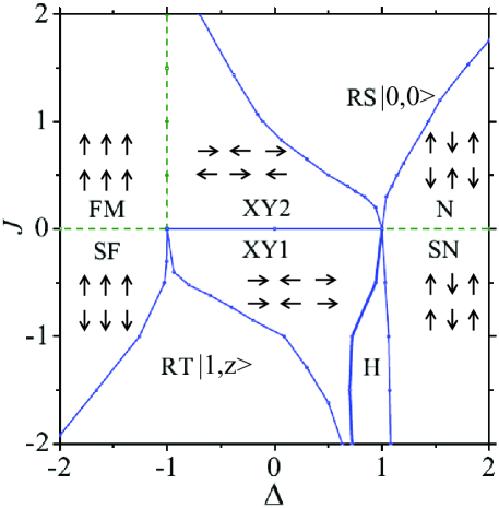
Figure 1: The groundstate phase diagram of the spin-${\textstyle\frac{1}{2}}$ $XXZ$ two-leg ladder model (1) in the $\Delta$–$J$ plane obtained from the groundstate fidelity and tensor network approach. The various lines denote the phase boundaries between the nine different phases. These are the ferromagnetic (FM), stripe ferromagnetic (SF), rung singlet (RS), rung triplet (RT), Néel (N), stripe Néel (SN), Haldane (H) and $XY$ ($XY1$ and $XY2$) phases. Dashed lines denote a first-order phase transition and solid lines denote a continuous phase transition.

2 The model

The fully anisotropic spin-${\textstyle\frac{1}{2}}$ $XXZ$ two-leg ladder system can be considered as a pair of infinitely long spin chains coupled via rung interactions. All spin interactions are of the spin-${\textstyle\frac{1}{2}}$ $XXZ$ Heisenberg type. The Hamiltonian is defined by

$$H=H_{\mathrm{leg}}+H_{\mathrm{rung}},$$ (1)

where

$$H_{\mathrm{leg}} = \sum_{i}\sum_{\alpha=1,2}\left(S_{\alpha,i}^{x}\,S_{\alpha,i+1}^{x}+S_{\alpha,i}^{y}\,S_{\alpha,i+1}^{y}+\Delta\,S_{\alpha,i}^{z}\,S_{\alpha,i+1}^{z}\right),$$ (2)

$$H_{\mathrm{rung}} = J\sum_{i}\left(S_{1,i}^{x}\,S_{2,i}^{x}+S_{1,i}^{y}\,S_{2,i}^{y}+\Delta\,S_{1,i}^{z}\,S_{2,i}^{z}\right).$$ (3)

Here $S_{\alpha,i}^{\beta}$ ($\beta=x,y,z$) is the spin-${\textstyle\frac{1}{2}}$ operator acting at site $i$ on the $\alpha$-th leg, $J$ is the rung coupling between the two spins on a rung, and $\Delta$ is the $XXZ$ anisotropy parameter. Our aim is to map out the groundstate phase diagram of this model in the $\Delta$–$J$ plane.

In the FM phase, the ladder system orders ferromagnetically in both the leg and rung directions, whereas in the SF phase it orders ferromagnetically in the leg direction and antiferromagnetically in the rung direction. In contrast, in the N phase, the system orders antiferromagnetically in both the leg and rung directions, whereas in the SN phase it orders antiferromagnetically in the leg direction and ferromagnetically in the rung direction. Notice that in the FM, SF, N, and SN phases $\langle S_{\alpha,i}^{x}\rangle=\langle S_{\alpha,i}^{y}\rangle=0$ and $\langle S_{\alpha,i}^{z}\rangle\neq 0$.

The critical $XY$ phases belong to the universality class of the Tomonaga-Luttinger liquid [39], which is known to exhibit a power-law decay of the spin-spin correlations with gapless excitations. The possibility for the existence of two different $XY$ phases in a ladder system was pointed out in a slightly different model [17]. According to the Marshall-Lieb-Mattis theorem [40], the $XY1$ phase is in the $J<0$ region and the $XY2$ phase is in the $J>0$ region of the parameter space. Long-range order does not exist in the $XY$ phases in the thermodynamic limit. Nevertheless, there is a practical way to characterize the $XY$ phases in the context of the TN representation of the groundstate wave functions, which is achieved by defining a pseudo-order parameter arising from the finiteness of the bond dimension $\chi$ [31]. This offers a convenient means to numerically determine the phase boundaries between the $XY$ phase and other phases. For the $XY1$ and $XY2$ phases, $\langle S_{\alpha,i}^{z}\rangle=0$ and $\langle S_{\alpha,i}^{x}\rangle^{2}+\langle S_{\alpha,i}^{y}\rangle^{2}\neq 0$.

The two-spin states on a rung are written as

$$|0,0\rangle = {1\over\sqrt{2}}(|\!\uparrow_{1}\downarrow_{2}\rangle-|\!\downarrow_{1}\uparrow_{2}\rangle),$$

$$|1,x\rangle = {1\over\sqrt{2}}(|\!\downarrow_{1}\downarrow_{2}\rangle-|\!\uparrow_{1}\uparrow_{2}\rangle),$$

$$|1,y\rangle = {{\mathrm{i}}\over\sqrt{2}}(|\!\downarrow_{1}\downarrow_{2}\rangle+|\!\uparrow_{1}\uparrow_{2}\rangle,$$

$$|1,z\rangle = {1\over\sqrt{2}}(|\!\uparrow_{1}\downarrow_{2}\rangle+|\!\downarrow_{1}\uparrow_{2}\rangle).$$

Here the subscripts $1$ and $2$ label the different spins on the same rung (see, e.g., Ref. [41]). The first state is the singlet and the remaining three states constitute the triplet. As can readily be seen from the Hamiltonian (1), the groundstate of the system in the strong coupling limit $J\to\pm\infty$ corresponds to the RS ($|0,0\rangle$) and RT ($|1,z\rangle$) phases, respectively. It should be noted that the RS phase, the RT phase and the H phase lack long-range order in the conventional Landau-Ginzburg-Wilson sense. However, each are characterized by a suitably modified string order parameter [42]. For the RS, RT and H phases $\langle S_{\alpha,i}^{\beta}\rangle=0$.

3 Results

To map out the groundstate phase diagram, we first consider the regions $J>0$ and $J<0$, with the anisotropy $\Delta$ as a control parameter. We then fix $\Delta$ and vary the rung coupling $J$. Illustrative examples are given in detail below for the values $J=\pm 1$. In our approach, apart from order parameters, which we also make use of, the groundstate fidelity per lattice site is used as an important tool to detect quantum phase transitions. For two different groundstates $|\psi(x)\rangle$ and $|\psi(x^{\prime})\rangle$ in a quantum system corresponding to different values $x$ and $x^{\prime}$ of a control parameter, the fidelity $F(x,x^{\prime})=|\langle\psi(x)|\psi(x^{\prime})\rangle|$ is defined as a measure of the overlap between the two states. For large but finite size $N$, the fidelity $F$ scales as $d^{N}$, with $d$ interpreted as the ground state fidelity per site $d=\lim_{N\rightarrow\infty}{F_{N}^{1/N}}$. As a well-defined property even in the thermodynamic limit, the groundstate fidelity per lattice site $d$ enjoys some properties inherited from the fidelity $F$, namely: (i) symmetry under interchange, $d(x,x^{\prime})=d(x^{\prime},x)$; (ii) normalization, $d(x,x)=1$; (iii) range $0\leq d(x,x^{\prime})\leq 1$.

In previous studies the fidelity per lattice site $d$ was demonstrated to be a useful detector for different types of quantum phase transition via its singularity structure [27, 28, 26, 29, 30, 31]. In this approach, a pinch point in the $d(x,x^{\prime})$ surface occurs at a quantum phase transition, i.e., at each phase transition point $x_{c}$, a pinch point $(x_{c},x_{c})$ occurs on the surface of fidelity per lattice site $d(x,x^{\prime})$ at the crossing of two singular lines $x=x_{c}$ and $x^{\prime}=x_{c}$. In these studies the groundstate wavefunctions are determined using TN algorithms [21, 43]. The combined groundstate fidelity and TN approach has been tailored to include ladder systems [20].

A key point in the investigation of the two-leg quantum spin ladders via the TN approach is that the computational cost scales as $\chi^{6}$, where $\chi$ is the bond dimension for each of the four necessary four-index tensors. These tensors need to be updated simultaneously, with the updating procedure closely related to the infinite PEPS [44] and translationally invariant MPS [45] algorithms. A summary of the TN approach for quantum spin ladders is given in Appendix A. For the spin-${\textstyle\frac{1}{2}}$ isotropic $XXX$ two-leg ladder it was demonstrated earlier that the TN approach could accurately determine the groundstate wave function, with bond dimension $\chi=6$ outperforming the DMRG results [20]. Of necessity for the calculation of the order parameters, the reduced density matrix $\rho$ can be computed directly from the TN representation of the groundstate wave functions [20]. The reduced density matrix displays different nonzero-entry structures in different phases.

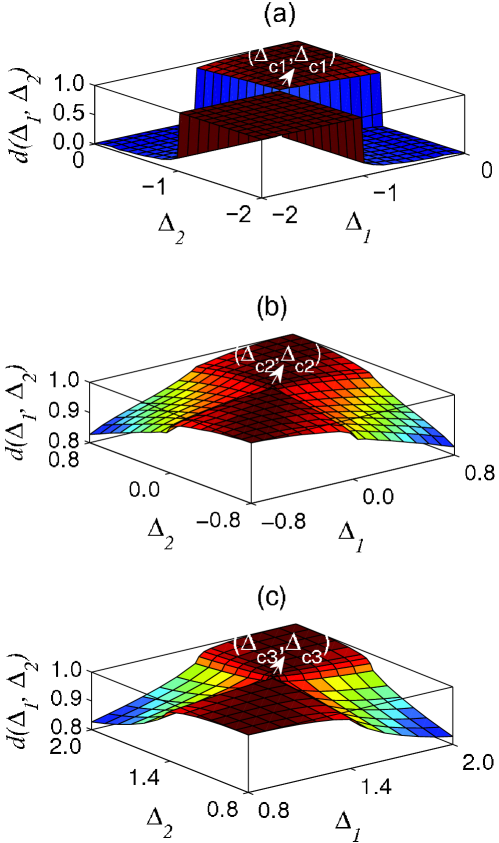
Figure 2: The groundstate fidelity surface $d(\Delta_{1},\Delta_{2})$ for the spin-${\textstyle\frac{1}{2}}$ $XXZ$ two-leg ladder model (1) for rung coupling $J=1$ and varying anisotropy $\Delta$ calculated with bond dimension $\chi=6$. Three pinch points are identified at $(\Delta_{c1},\Delta_{c1})$, $(\Delta_{c2},\Delta_{c2})$ and $(\Delta_{c3},\Delta_{c3})$ on the global fidelity surface, indicating three phase transition points, located at (a) $\Delta_{c1}=-1.00$, (b) $\Delta_{c2}=0.00$ and (c) $\Delta_{c3}=1.43$.

3.1 $J=1,-2\leq\Delta\leq 2$

Fixing the rung coupling to the value $J=1$ and varying the anisotropy parameter $\Delta$ from $-2$ to $2$, we are able to determine the phase boundaries between the FM phase, the $XY2$ phase, the RS phase and the Néel phase. The groundstate fidelity per site, $d(\Delta_{1},\Delta_{2})$, is shown in Figure 2 as a function of $\Delta_{1}$ and $\Delta_{2}$, calculated with bond dimension $\chi=6$. Here the range of the plots is restricted to highlight the fidelity surface and, in particular, the pinch points. The results in Figure 2(a) and Figure 2(c) differ very little for a larger bond dimension $\chi$, indicating that the computational results are almost saturated for bond dimension $\chi=6$. However, the pinch point in Figure 2(b) shifts noticeably when $\chi$ increases from $\chi=6$ to $\chi=12$, as Figure 3 shows. Three pinch points are identified at $(\Delta_{c1},\Delta_{c1})$, $(\Delta_{c2},\Delta_{c2})$ and $(\Delta_{c3},\Delta_{c3})$ on the fidelity surfaces, indicating that there are three phase transition points. These are located at (i) $\Delta_{c1}=-1.00$, (ii) $\Delta_{c2}=0.00$ and (iii) $\Delta_{c3}=1.43$. In this way we are able to identify four different phases, separated by three transition points. It remains to characterize these phases in terms of local or nonlocal order parameters.

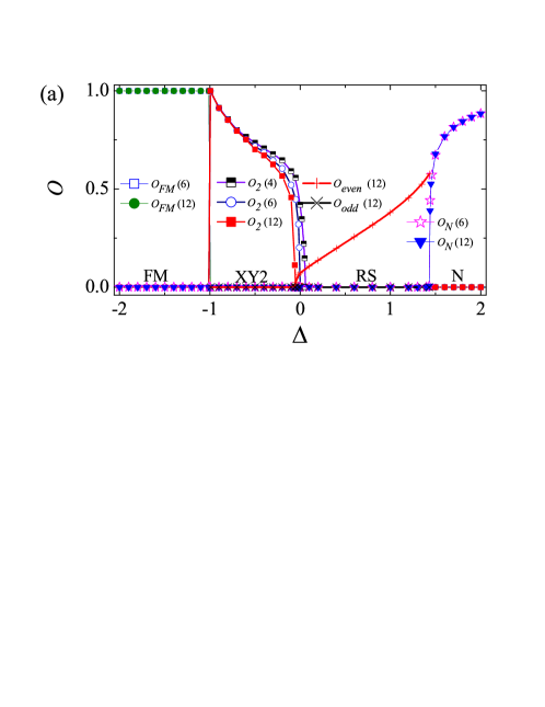
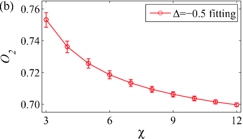
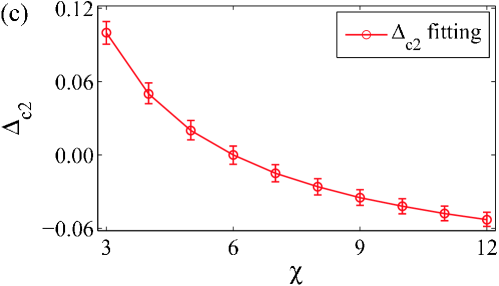
Figure 3: (a) The local order parameter $O_{\mathrm{FM}}(\chi)$ in the FM phase, the pseudo-order parameter $O_{2}(\chi)$ in the $XY2$ phase, the local order parameter $O_{\mathrm{N}}(\chi)$ in the Néel phase and the string order parameters $O_{\mathrm{odd}}(\chi)$ and $O_{\mathrm{even}}(\chi)$ in the RS phase as a function of the anisotropy $\Delta$, with $J=1$. Three phase transition points, $\Delta_{c1}$, $\Delta_{c2}$ and $\Delta_{c3}$, are distinguished by the behavior of the order parameters. The phase transition points $\Delta_{c1}=-1.00$ and $\Delta_{c3}=1.43$ are saturated for bond dimension $\chi=6$, whereas $\Delta_{c2}$ shifts with increasing $\chi$. (b) The scaling of the pseudo-order parameter $O_{2}(\chi)$ for $\Delta=-0.5$ (see text). (c) The “pseudo-critical” point estimates $\Delta_{c2}(\chi)$ obtained from the pseudo-order parameter $O_{2}(\chi)$ and their fitting function (see text).

In the FM phase, the one-site reduced density matrix yields the local order parameter,

$$O_{\mathrm{FM}}=\frac{1}{2}|\langle(S^{z}_{1,i}+S^{z}_{2,i})+(S^{z}_{1,i+1}+S^{z}_{2,i+1})\rangle|.$$ (4)

Our numerical results indicate that the ladder system is in the FM phase for $\Delta<-1.00$ (see Figure 3(a)).

In the Néel phase, we similarly consider the local order parameter

$$O_{\mathrm{N}}=\frac{1}{2}|\langle(S^{z}_{1,i}-S^{z}_{2,i})-(S^{z}_{1,i+1}-S^{z}_{2,i+1})\rangle|.$$ (5)

In the Néel phase, the Néel order $O_{\mathrm{N}}$ exhibits a long-range order. The evaluation of the order parameter indicates that the ladder system is in the Néel phase for $\Delta>1.43$ (see Figure 3(a)).

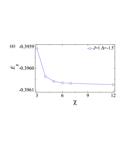
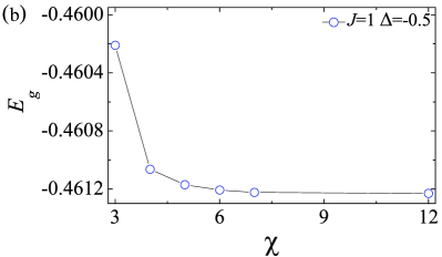
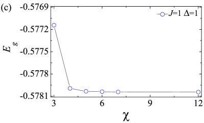
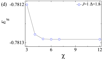
Figure 4: Convergence of the groundstate energy $E_{g}$ with increasing bond dimension $\chi=3,4,5,6,7,12$ in different phases with rung coupling $J=1$ and anisotropy parameter values (a) $\Delta=-1.5$ (FM phase) (b) $\Delta=-0.5$ ($XY2$ phase) (c) $\Delta=1.0$ (RS phase) (d) $\Delta=1.8$ (N phase).

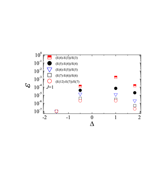
Figure 5: Relative error $\varepsilon$ in the estimates of the groundstate energy as a function of $\Delta$ at $J=1$ for increasing bond dimension $\chi$. The relative errors are defined by $\varepsilon=(E(\chi_{n+1})-E(\chi_{n}))/E(\chi_{n})$ where $E(\chi_{n})$ is the groundstate energy estimate for given bond dimension $\chi_{n}$.

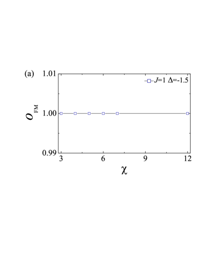
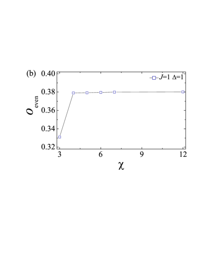
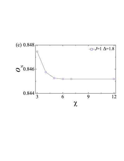
Figure 6: Convergence of order parameters with increasing bond dimension $\chi=3,4,5,6,7,12$ in different phases for $J=1$. (a) local order parameter $O_{\mathrm{FM}}$ for $\Delta=-1.5$ (FM phase). (b) string order parameter $O_{\mathrm{even}}$ for $\Delta=1.0$ (RS phase). (c) local order parameter $O_{\mathrm{N}}$ for $\Delta=1.8$ (N phase).

In the RS phase, the groundstate wave function may be approximated by the product of local rung singlets. As usual, two distinct string order parameters, $O_{\mathrm{odd}}$ and $O_{\mathrm{even}}$, may be used to characterize the RS phase. For two-leg ladder models these are defined by

$$O_{{\mathrm{odd}}/{\mathrm{even}}}=-\lim_{\left|i-j\right|\to\infty}\Big{\langle}S_{{\mathrm{o}}/{\mathrm{e}},i}^{z}\exp\Big{[}\mathrm{i}\pi\sum_{l=i+1}^{j-1}S_{{\mathrm{o}}/{\mathrm{e}},l}^{z}\Big{]}S_{{\mathrm{o}}/{\mathrm{e}},j}^{z}\Big{\rangle},$$ (6)

where $S^{z}_{{\mathrm{o}},i}\equiv S^{z}_{1,i}+S^{z}_{2,i}$ and $S^{z}_{{\mathrm{e}},i}\equiv S^{z}_{1,i}+S^{z}_{2,i+1}$. The odd and even string order parameters are actually mutually exclusive in the RS, RT and H phases. Our results for $O_{\mathrm{odd}}$ and $O_{\mathrm{even}}$ indicate that the RS phase persists in the region $\Delta_{c2}<\Delta<\Delta_{c3}$ with $J=1$ (see Figure 3(a)).

In the $XY$ phases, the TN algorithm automatically leads to infinite degenerate groundstates, arising from pseudo spontaneous symmetry breaking of the continuous U(1) symmetry, due to the finiteness of the bond dimension $\chi$. This allows the introduction of a pseudo-order parameter that must scale to zero, in order to keep consistency with the Mermin-Wagner theorem. As suggested in Refs. [31] and [41], the pseudo-order parameters in the $XY1$ and $XY2$ phases may be defined as

$$O_{1}=\sqrt{\langle S^{x}_{1,i}+S^{x}_{2,i}\rangle^{2}+\langle S^{y}_{1,i}+S^{y}_{2,i}\rangle^{2}},$$ (7)

and

$$O_{2}=\sqrt{\langle S^{x}_{1,i}-S^{x}_{2,i}\rangle^{2}+\langle S^{y}_{1,i}-S^{y}_{2,i}\rangle^{2}}.$$ (8)

The pseudo-order parameter $O_{2}$ in the $XY2$ phase is plotted as a function of the anisotropy $\Delta$ for different values of the bond dimension $\chi$ in Figure 3(a). This order parameter $O_{2}$ is also plotted as a function of $\chi$ for $\Delta=-0.5$ in Figure 3(b). It is clearly seen that $O_{2}$ decreases as $\chi$ increases. Here the pseudo-order parameter scales to zero according to $O_{2}(\chi)=a_{1}\,\chi^{-b_{1}}(1+c_{1}\,\chi^{-1})$, with $a_{1}=0.697(3)$, $b_{1}=0.007(1)$ and $c_{1}=0.26(1)$. Such scaling was adopted in previous studies of pseudo-order parameters [31, 41] and ensures that they vanish for infinite bond dimension as expected.

The estimates of the “pseudo-critical” values $\Delta_{c2}(\chi)$ at which the pseudo-order parameter $O_{2}(\chi)$ becomes zero are shown in Figure 3(c). These points are extrapolated with respect to the bond dimension $\chi$, with an extrapolation function $\Delta(\chi)=a_{2}+b_{2}\,\chi^{-c_{2}}$. The results imply the fitting constants $a_{2}=-0.110(2)$, $b_{2}=0.585(7)$ and $c_{2}=0.93(2)$. In the limit $\chi\rightarrow\infty$ we have $\Delta(\infty)=a_{2}$, which is the estimate for the critical point $\Delta_{c2}$ between the $XY2$ and RS phases. The term “pseudo-critical” point is used because such estimates are obtained using the pseudo-order parameters. Nevertheless they yield estimates for real critical points.

The existence of the FM phase, the $XY2$ phase, the Néel phase and the RS phase is numerically confirmed in this way, as seen from Figure 3. Specifically, the three phase transition points occur at the values $\Delta_{c1}=-1.00$, $\Delta_{c2}\simeq-0.11$ and $\Delta_{c3}=1.43$. If the anisotropy coupling $\Delta$ is tuned as a control parameter, the ladder system undergoes a first-order phase transition at $\Delta_{c1}$, with continuous phase transitions at $\Delta_{c2}$ and $\Delta_{c3}$. The different nature of the first-order transition at $\Delta_{c1}$ can be seen clearly in the fidelity surface in Figure 2(a), compared to the continuous transitions in Figure 2(b) and Figure 2(c). In general, for continuous phase transitions, the fidelity surface shows continuous behaviour near critical points, while discontinuous phase transitions show discontinuous behaviour.

In the limit $J\rightarrow\infty$ the $XY2$ phase vanishes. In addition for general $J>0$ the line $\Delta=-1$ is the phase boundary between the FM phase $\Delta<-1$ and the $XY2$ phase $\Delta>-1$. We have also confirmed that $\Delta\approx J$ is the phase boundary between the RS phase and the Néel phase, when $\Delta\rightarrow\infty$ and $J\rightarrow\infty$. There are thus three phases when $J\rightarrow\infty$: the FM phase, the RS phase and the Néel phase.

Concerning the accuracy of our results, estimates of the groundstate energy per site with increasing bond dimension are shown in Figure 4. The estimates are seen to converge rapidly, as quantified in Figure 5. We find that almost all of the relative errors reach to order $10^{-5}$. This indicates the reliability of the algorithm for generating accurate groundstate wave functions for spin ladders, given a preset error tolerance. The corresponding convergence of the order parameter estimates is shown in Figure 6. As is well understood, states in gapless phases, such as the $XY1$ and $XY2$ phases, are more difficult to compute than states in phases with a large gap, such as the FM, N and SF phases, which converge much faster, yielding the same accuracy with a smaller bond dimension. Phases with a small gap, such as the H phase, are also more difficult to compute. In general this slower convergence in gapless (critical) versus gapped phases is a feature of numerical entanglement based approaches, such as TN methods [43]. This is because the overall strategy of the TN method is more efficient for gapped systems. By design, the finite bond dimension already induces a gap in the system. From the perspective of entanglement in quantum critical phenomena [46], gapped systems obey an area law, which can be well described using relatively small bond dimensions. On the other hand, for gapless systems, the entanglement diverges as the gap vanishes, requiring larger, in principle infinite, bond dimensions. Alternatively, for the same size bond dimension, more iteration steps are necessary for convergence in gapless compared to gapped systems. Our algorithm is seen to work sufficiently well in the phases under consideration. However, the critical $XY1$ and $XY2$ phases require additional extrapolation to infinite-size bond dimension.

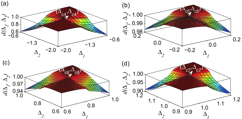
Figure 7: The groundstate fidelity surface $d(\Delta_{1},\Delta_{2})$ for the spin-${\textstyle\frac{1}{2}}$ $XXZ$ two-leg ladder model (1) for rung coupling $J=-1$ and varying anisotropy $\Delta$ calculated with bond dimension $\chi=6$. Four pinch points are identified at $(\Delta_{c4},\Delta_{c4})$, $(\Delta_{c5},\Delta_{c5})$, $(\Delta_{c6},\Delta_{c6})$ and $(\Delta_{c7},\Delta_{c7})$ on the global fidelity surface, indicating four phase transition points, located at (a) $\Delta_{c4}=-1.26$, (b) $\Delta_{c5}=0.00$, (c) $\Delta_{c6}=0.84$, and (d) $\Delta_{c7}=1.06$.

3.2 $J=-1,-2\leq\Delta\leq 2$

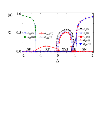
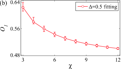
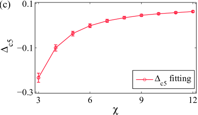
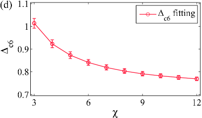
Figure 8: (a) The local order parameters $O_{\mathrm{SF}}$ in the SF phase and $O_{\mathrm{SN}}$ in the SN phase, the pseudo-order parameter $O_{1}$ in the $XY1$ phase and the string order parameters $O_{\mathrm{odd}}$ and $O_{\mathrm{even}}$ in the Haldane and RT ($|1,z\rangle$) phases as a function of the anisotropy $\Delta$, with $J=-1$. Two phase transition points are identified at $\Delta_{c4}=-1.26$ and $\Delta_{c7}=1.06$ for $\chi=6$, with no significant shift observed for increasing $\chi$. The other two phase transition estimates, $\Delta_{c5}$ and $\Delta_{c6}$, shift with increasing $\chi$. (b) The pseudo-order parameter estimates $O_{1}(\chi)$ for $\Delta=0.5$ in the $XY1$ phase (see text). (c) The “pseudo-critical” point estimates $\Delta_{c5}(\chi)$ obtained from the pseudo-order parameter $O_{1}(\chi)$ and its fitting function (see text). (d) The “pseudo-critical” point estimates $\Delta_{c6}(\chi)$ obtained from the pseudo-order parameter $O_{1}(\chi)$ and its fitting function (see text).

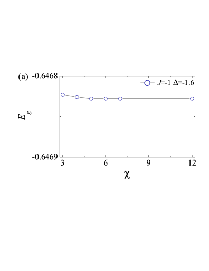
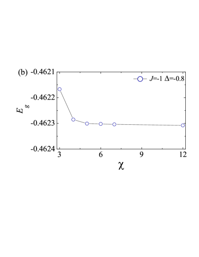
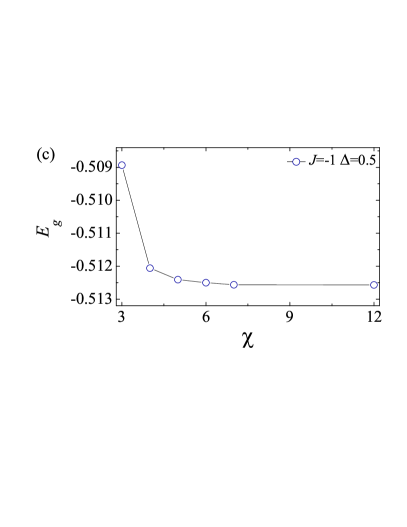
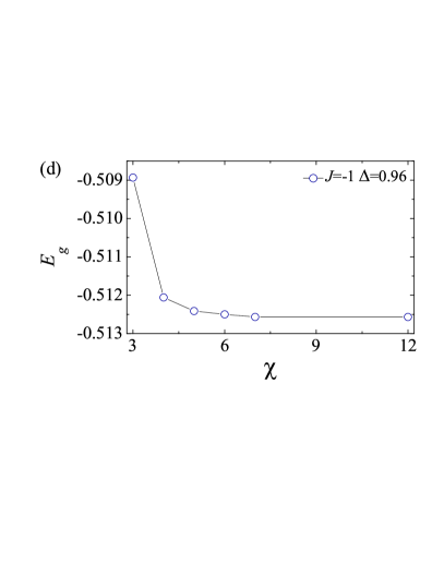
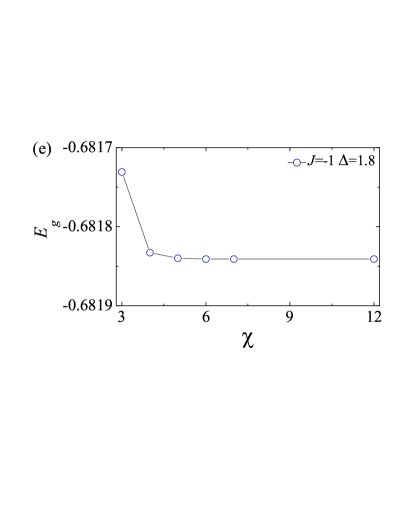
Figure 9: Convergence of the groundstate energy $E_{g}$ with increasing bond dimension $\chi=3,4,5,6,7,12$ in different phases with rung coupling $J=-1$ and anisotropy parameter values (a) $\Delta=-1.6$ (SF phase) (b) $\Delta=-0.8$ (RT phase) (c) $\Delta=0.5$ ($XY1$ phase) (d) $\Delta=0.96$ (Haldane phase) (e) $\Delta=1.8$ (SN phase).

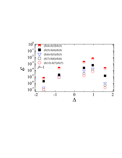
Figure 10: Relative error $\varepsilon$ in the estimates of the groundstate energy as a function of $\Delta$ at $J=-1$ for increasing bond dimension $\chi$. The relative errors are defined by $\varepsilon=(E(\chi_{n+1})-E(\chi_{n}))/E(\chi_{n})$ where $E(\chi_{n})$ is the groundstate energy estimate for given bond dimension $\chi_{n}$.

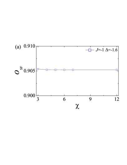
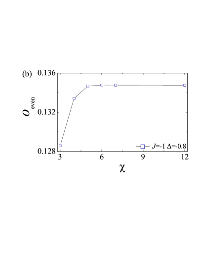
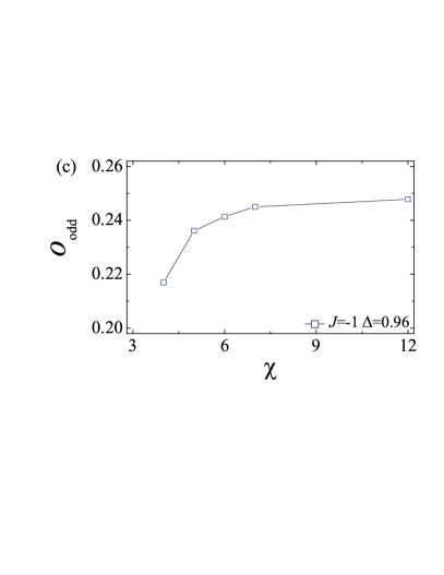
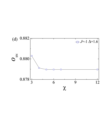
Figure 11: Convergence of order parameters with increasing bond dimension $\chi=3,4,5,6,7,12$ in different phases for $J=-1$. (a) local order parameter $O_{\mathrm{SF}}$ for $\Delta=-1.6$ (SF phase). (b) string order parameter $O_{\mathrm{even}}$ for $\Delta=0.8$ (RT phase). (c) string order parameter $O_{\mathrm{odd}}$ for $\Delta=0.96$ (H phase). (d) local order parameter $O_{\mathrm{SN}}$ for $\Delta=1.6$ (SN phase).

In similar fashion, we determine the phase boundaries between the SF, RT ($|1,z\rangle$), $XY1$, H and SN phases. The groundstate fidelity per lattice site $d(\Delta_{1},\Delta_{2})$ is shown as a function of $\Delta_{1}$ and $\Delta_{2}$ in Figure 7 with bond dimension $\chi=6$. In this region four pinch points, $(\Delta_{c4},\Delta_{c4})$, $(\Delta_{c5},\Delta_{c5})$, $(\Delta_{c6},\Delta_{c6})$ and $(\Delta_{c7},\Delta_{c7})$, are identified on the fidelity surfaces, corresponding to the continuous phase transition points $\Delta_{c4}=-1.26$, $\Delta_{c5}=0.00$, $\Delta_{c6}=0.84$ and $\Delta_{c7}=1.06$. These points separate five different phases, which we now proceed to characterize in terms of the order parameters.

In the SF phase, the one-site reduced density matrix yields the local order parameter

$$O_{\mathrm{SF}}=\frac{1}{2}|\langle(S^{z}_{1,i}-S^{z}_{2,i})+(S^{z}_{1,i+1}-S^{z}_{2,i+1})\rangle|.$$ (9)

Our results show that the ladder system exhibits a long-range order in the SF phase for $\Delta<-1.26$ (see Figure 8(a)).

In the SN phase, we are similarly able to consider the local order parameter

$$O_{\mathrm{SN}}=\frac{1}{2}|\langle(S^{z}_{1,i}+S^{z}_{2,i})-(S^{z}_{1,i+1}+S^{z}_{2,i+1})\rangle|.$$ (10)

In this phase the ladder system exhibits a long-range order for $\Delta>1.06$ (see Figure 8(a)).

In the H phase, the even string order parameter $O_{\mathrm{even}}$ vanishes, but the odd string order parameter is nonzero. Conversely, in the RT ($|1,z\rangle$) phase, $O_{\mathrm{odd}}=0$ and the even string order parameter is nonzero (see Figure 8(a)).

In the $XY1$ phase, the pseudo-order parameter $O_{1}$ as a function of the anisotropy $\Delta$ for different bond dimension $\chi$ is shown in Figure 8(a). The pseudo-order parameter is plotted as a function of $\chi$ for $\Delta=0.5$ in Figure 8(b). Here we have performed an extrapolation with respect to $\chi$, with the fitting function $O_{1}(\chi)=a_{3}\,\chi^{-b_{3}}(1+c_{3}\,\chi^{-1})$, where $a_{3}=0.467(7)$, $b_{3}=0.006(4)$ and $c_{3}=1.04(5)$. This is again consistent with previous studies of pseudo-order parameters. The estimates of the “pseudo-critical” points $\Delta_{c5}(\chi)$ and $\Delta_{c6}(\chi)$ on either side of the $XY1$ phase are shown in Figure 8(c) and Figure 8(d). Here we employ the extrapolation functions $\Delta_{c5}(\chi)=a_{4}+b_{4}\,\chi^{-c_{4}}$ and $\Delta_{c6}(\chi)=a_{5}+b_{5}\,\chi^{-c_{5}}$. Numerical fitting yields $a_{4}=0.088(2)$, $b_{4}=-2.54(7)$ and $c_{4}=1.88(2)$ for the phase transition between the RT ($|1,z\rangle$) and $XY1$ phases with the values $a_{5}=0.718(2)$, $b_{5}=1.18(4)$ and $c_{5}=1.26(3)$ for the phase transition between the $XY1$ and H phases. In the limit $\chi\rightarrow\infty$ this yields the two critical point estimates $\Delta_{c5}$ and $\Delta_{c6}$.

It follows that we have been able to compute the order parameters $O_{\mathrm{SF}}$ and $O_{\mathrm{SN}}$ in the SF and SN phases, the pseudo-order parameter $O_{1}$ in the $XY1$ phase, the string order parameter $O_{\mathrm{even}}$ in the RT ($|1,z\rangle$) phase, and the string order parameter $O_{\mathrm{odd}}$ in the H phase. The results are shown in Figure 8. With the anisotropy $\Delta$ as control parameter, the ladder system undergoes four continuous phase transitions at the values $\Delta_{c4}$, $\Delta_{c5}$, $\Delta_{c6}$ and $\Delta_{c7}$.

In the limit $J\rightarrow-\infty$ the $XY1$ phase and the H phase vanish. We note that the phase boundary between the SF phase and the RT ($|1,z\rangle$) phase is located roughly near the line $\Delta\approx J$ in the limits $\Delta\rightarrow-\infty$ and $J\rightarrow-\infty$, while the phase boundary between the RT ($|1,z\rangle$) and SN phases is located roughly near the line $\Delta\sim 1$ as $J\rightarrow-\infty$. As a result there are three phases for the ladder system in the limit $J\rightarrow-\infty$, i.e., the SF, RT ($|1,z\rangle$) and SN phases.

The accuracy of the results is similar to that for $J>0$, with estimates of the groundstate energy per site with increasing bond dimension shown in Figure 9. The estimates also converge rapidly, as quantified in Figure 10. The corresponding convergence of the order parameter estimates is shown in Figure 11.

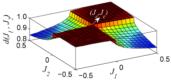
Figure 12: The groundstate fidelity surface $d(J_{1},J_{2})$ for the spin-${\textstyle\frac{1}{2}}$ $XXZ$ two-leg ladder model (1) for anisotropy parameter $\Delta=0$ and varying rung coupling with bond dimension $\chi=6$. The pinch point occurring at $(J_{c}=0.00,J_{c}=0.00)$ indicates a continuous phase transition point.

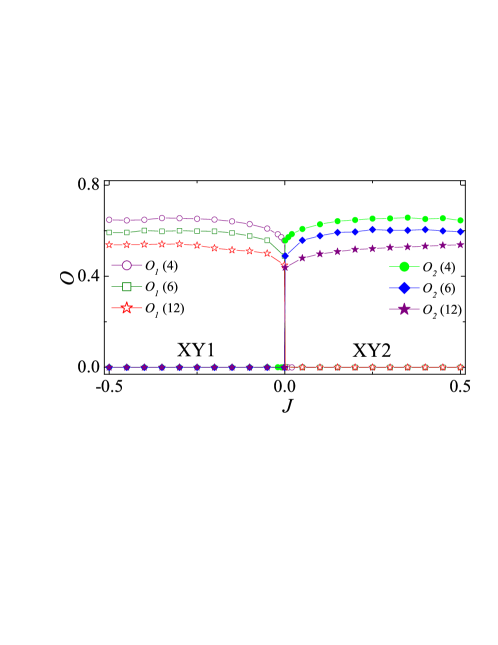
Figure 13: The pseudo-order parameter $O_{1}(\chi)$ in the $XY1$ phase and the pseudo-order parameter $O_{2}(\chi)$ in the $XY2$ phase as a function of the rung coupling $J$. The bond dimension values are $\chi=4,6,12$.

3.3 $\Delta=0,-0.5\leq J\leq 0.5$

We now turn to look more closely at the $XY$ phase, which as we have seen, splits into the two different $XY1$ and $XY2$ phases identified by the local pseudo-order parameters $O_{1}$ and $O_{2}$ obtained from the groundstate fidelity per lattice site. As we shall see, for $-1\leq\Delta\leq 1$, the phase boundary between the $XY1$ and $XY2$ phases is the line $J=0$. Here we fix the anisotropy coupling $\Delta=0$ and take $J$ as control parameter in the range $-0.5\leq J\leq 0.5$ to sweep across this boundary.

Figure 12 shows a plot of the groundstate fidelity per site $d(J_{1},J_{2})$ with bond dimension $\chi=6$. In this case there is a clear indication of a continuous phase transition point at $J=0.00$, as a pinch point occurs at this value with bond dimension $\chi=6$. Figure 13 shows a plot of the pseudo-order parameter $O_{1}$ in the $XY1$ phase and the pseudo-order parameter $O_{2}$ in the $XY2$ phase as a function of $J$. As already remarked, a feature of the pseudo-order parameters is that they vanish as the bond dimension $\chi$ increases.

4 Conclusion

We have systematically investigated the groundstate phase diagram of the infinite fully anisotropic spin-${\textstyle\frac{1}{2}}$ $XXZ$ two-leg ladder model (1). This has been achieved by exploiting a TN algorithm tailored to the geometry of quantum spin ladder systems [20], allowing efficient evaluation of the groundstate fidelity per lattice site from the TN representation of the groundstate wave functions for the infinite-size quantum spin ladder. Illustrative results have been presented in Sec. III along the lines $J=\pm 1$ with varying $\Delta$ and the line $\Delta=0$ with varying $J$. Our computational results using the groundstate fidelity per lattice site are consistent with results obtained from the construction of local, and where appropriate, nonlocal, order parameters in the different phases.

The full phase diagram, as obtained by this approach, is shown in Figure 1. This phase diagram, featuring nine distinct quantum phases, points to the rich diversity of physics in the fully anisotropic spin-${\textstyle\frac{1}{2}}$ $XXZ$ two-leg ladder model. The precise nature of the phase diagram is a significant extension on the previously obtained schematic phase diagram for this model, which was mapped out by identifying ridges and valleys in contour plots of the rescaled block entanglement entropy corresponding to possible phase boundaries [37]. With that approach, which was aimed at demonstrating the usefulness of sublattice entanglement entropy as a means of exploring quantum phase transitions across a range of different spin systems, the nature and number of the different phases of the ladder model were not discussed in detail. The phase diagram of the fully anisotropic spin-${\textstyle\frac{1}{2}}$ $XXZ$ two-leg ladder model also differs in significant aspects compared to the phase diagram of the spin-${\textstyle\frac{1}{2}}$ $XXZ$ two-leg ladder model with isotropic rung interactions, the precise nature of which has been the subject of debate [9, 38]. With isotropic rung interactions, the model also exhibits FM, SF, RS, N, SN, H, $XY1$ and $XY2$ phases. However, for the fully anisotropic model considered here, there is an additional rung-triplet (RT($|1,z\rangle$)) phase, with the $XY1$ and $XY2$ phases extending over the whole $-1\leq\Delta\leq 1$ region in the vicinity of $J\approx 0$. Moreover, the extent of the Haldane (H) phase is seen to be significantly diminished for fully anisotropic interactions. In general the difference between both the number of quantum phases and the phase diagrams of the two models highlights the key role played by anisotropies in the competition between singlet formation and magnetic ordering in quantum spin systems.

Appendix A Tensor network representation for the spin-${\textstyle\frac{1}{2}}$ two-leg ladder

In this Appendix we summarise the relevant details of the TN representation for spin ladders [20]. The hamiltonian of the two-leg ladder model (1) under consideration is of the general form $H=\sum_{i}h_{i}$, with $h_{i}$ acting on the $i$th plaquette between sites $i$ and $i+1$ along a leg. The index $i$ runs over all possible plaquettes with $i\in\{-\infty,\ldots,+\infty\}$. It is sufficient to assume that the TN representation for the wave function is translational invariant under shifts by two lattice sites along the legs. The groundstate wave function for an infinite length ladder can be described by the four different four-index tensors $A_{\ell rd}^{s}$, $B_{\ell rd}^{s}$, $C_{\ell ru}^{s}$ and $D_{\ell ru}^{s}$. The tensor $A_{\ell rd}^{s}$ is depicted in Figure 14(i), with $s=1,2$ for spin-${\textstyle\frac{1}{2}}$ and with $\ell$, $r$, $u$, $d=1,\ldots,\chi$, the four inner bond indices, where $\chi$ is the bond dimension. A TN representation for the groundstate wave function is shown in Figure 14(ii) with one of the two equivalent choices shown for the plaquette (unit cell).

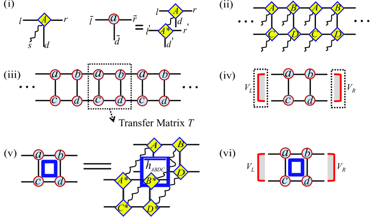
Figure 14: (i) Four-index tensor $A^{s}_{lrd}$ used in the TN representation for the groundstate wave function for the infinite-size two-leg spin ladder. Also shown is the double tensor $a_{\tilde{\ell}\tilde{r}\tilde{d}}$ formed from the tensor $A_{\ell rd}^{s}$ and its complex conjugate ${(A^{*})_{\ell^{\prime}r^{\prime}d^{\prime}}^{s}}$, with $\tilde{\ell}=(\ell,\ell^{\prime})$, $\tilde{r}=(r,r^{\prime})$ and $\tilde{d}=(d,d^{\prime})$. (ii) Pictorial representation for a TN state ${|\psi\rangle}$ with leg and rung bonds, which are used to absorb an operator acting on the $i$th plaquette. (iii) TN representation for the norm of a groundstate wavefunction in the infinite ladder. Also shown is the transfer matrix $T$, which is constructed from the four double tensors $a_{\tilde{\ell}\tilde{r}\tilde{d}}$, $b_{\tilde{\ell}\tilde{r}\tilde{d}}$, $c_{\tilde{\ell}\tilde{r}\tilde{u}}$ and $d_{\tilde{\ell}\tilde{r}\tilde{u}}$, with $\tilde{\ell}$, $\tilde{r}$ and $\tilde{d}$ defined as above and $\tilde{u}=(u,u^{\prime})$. (iv) The dominant left and right eigenvectors $V_{L}$ and $V_{R}$ of the transfer matrix $T$. (v) A unit cell with hamiltonian density $h_{ABDC}$ acting on the plaquette ABDC. (iv) The groundstate energy per unit cell is computed from the eigenvectors $V_{L}$, $V_{R}$ and the tensors $A_{\ell rd}^{s}$, $B_{\ell rd}^{s}$, $C_{\ell ru}^{s}$ and $D_{\ell ru}^{s}$.

A gradient-directed random walk method is applied to compute the groundstates. The double tensors $a_{\tilde{\ell}\tilde{r}\tilde{d}}$, $b_{\tilde{\ell}\tilde{r}\tilde{d}}$, $c_{\tilde{\ell}\tilde{r}\tilde{u}}$ and $d_{\tilde{\ell}\tilde{r}\tilde{u}}$ are introduced, with $\tilde{\ell}=(\ell,\ell^{\prime})$, $\tilde{r}=(r,r^{\prime})$, $\tilde{u}=(u,u^{\prime})$ and $\tilde{d}=(d,d^{\prime})$. They are formed from the tensors $A_{\ell rd}^{s}$, $B_{\ell rd}^{s}$, $C_{\ell ru}^{s}$ and $D_{\ell ru}^{s}$, and their complex conjugates, as depicted in Figure 14(i) for the double tensor $a$. With these double tensors, the TN for the norm of a wave function is shown in Figure 14(iii). The two different but equivalent choices for the transfer matrix $T$ are made from the plaquettes $abdc$ and $bacd$. In the above, the notation $\tilde{\ell}=(\ell,\ell^{\prime})$ corresponds to the two independent indices $\ell$ and $\ell^{\prime}$, with $\tilde{\ell}=1,2,\ldots,\chi^{2}$. Similarly for $\tilde{r}$, $\tilde{u}$ and $\tilde{d}$.

For a randomly chosen initial state $|\psi_{0}\rangle$, the energy per plaquette $e$ is

$$e=\frac{\langle\psi_{0}|(h_{ABDC}+h_{BACD})|\psi_{0}\rangle}{2\langle\psi_{0}|\psi_{0}\rangle}.$$ (11)

The groundstate energy per plaquette also admits a TN representation as shown in Figure 14(v) and (vi) for plaquette ABDC, which absorbs the operator $h$ acting on a plaquette for an infinite-size spin ladder. For each choice of plaquette, the dominant left and right eigenvectors of the transfer matrix $T$ constitute the environment tensors, visualised in Figure 14(iv) and (vi) for plaquette ABDC. In this way the energy per plaquette $e_{ABDC}$ is obtained. The same procedure may be used to compute the energy per plaquette $e_{BACD}$ for an operator acting on the $i$th plaquette BACD.

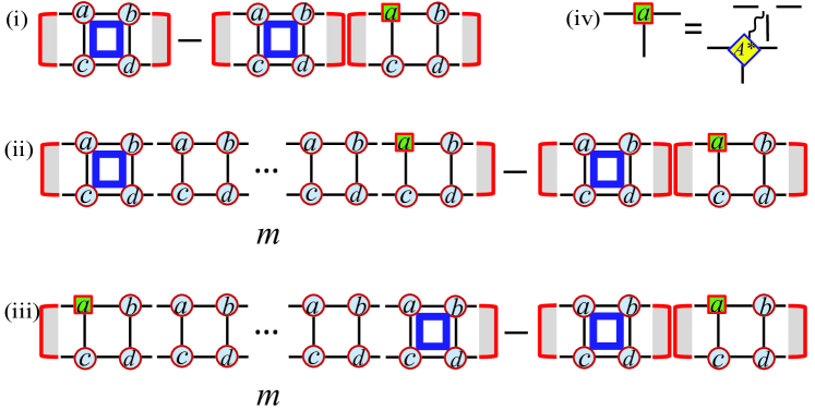
Figure 15: The contribution to the energy gradient (12) for the infinite-size spin ladder consists of three parts: (i), (ii) and (iii) depending on the location of the hole cell with tensor $A_{\ell rd}^{s}$ removed. In the latter two cases, there are $m$ cells between the hole and hamiltonian cell, where $m\in(0,1,2,3,\ldots)$. The hole cell is visualised in (iv), with the tensor $A_{\ell rd}^{s}$ removed. Note that only the contribution from the plaquette $abdc$, as labeled here, is shown. There is also a similar contribution from the plaquette $bacd$.

To update the TN representation, the energy gradient is computed with respect to the tensor $A_{\ell rd}^{s}$, with

$$\frac{\partial{e}}{\partial A_{\ell rd}^{s}}=\frac{{\partial\langle\psi_{0}|H|\psi_{0}\rangle}/{\partial A_{\ell rd}^{s}}}{\langle\psi_{0}|\psi_{0}\rangle}-{E_{g}}\,\frac{{\partial\langle\psi_{0}|\psi_{0}\rangle}/{\partial A_{\ell rd}^{s}}}{\langle\psi_{0}|\psi_{0}\rangle}.$$ (12)

The contributions to the energy gradient come from three parts (for a given choice of plaquette on which the hamiltonian acts), as shown in Figure 15. To obtain the energy gradient it is necessary to sum the contributions from both plaquettes $abdc$ and $bacd$. The tensor $A_{\ell rd}^{s}$ is then updated according to

$$A_{\ell rd}^{s}=A_{\ell rd}^{s}-\delta\;\frac{\partial{E_{g}}/\partial A_{\ell rd}^{s}}{\max_{(\ell,r,d)}\mid\partial{E_{g}}/\partial A_{\ell rd}^{s}\mid},$$ (13)

where $\delta$ denotes the update step size. In this procedure the tensors $A_{\ell rd}^{s}$, $B_{\ell rd}^{s}$, $C_{\ell ru}^{s}$ and $D_{\ell ru}^{s}$ are updated simultaneously. Repeating this procedure until the groundstate energy per plaquette converges leads to the groundstate wave function as approximated in the TN representation.

References

References

- [1] Dagotto E and Rice T M 1996 Surprises on the way from one- to two-dimensional quantum magnets: The ladder materials Science 271 618 Dagotto E 1999 Experiments on ladders reveal a complex interplay between a spin-gapped normal state and superconductivity Rep. Prog. Phys. 62 1525
- [2] Batchelor M T, Guan X-W, Oelkers N and Tsuboi Z 2007 Integrable models and quantum spin ladders: comparison between theory and experiment for the strong coupling ladder compounds Adv. Phys. 56 465
- [3] White S R, Noack R M and Scalapino D J 1994 Resonating valence-bond theory of coupled Heisenberg-chains Phys. Rev. Lett. 73 886
- [4] Shelton D G, Nersesyan A A and Tsvelik A M 1996 Antiferromagnetic spin ladders: Crossover between spin and chains Phys. Rev. B 53 8521
- [5] Nersesyan A A and Tsvelik A M 1997 One-dimensional spin-liquid without magnon excitations Phys. Rev. Lett. 78 3939
- [6] Fouet J-B, Mila F, Clarke D, Youk H, Tchernyshyov O, Fendley P and Noack R M 2006 Condensation of magnons and spinons in a frustrated ladder Phys. Rev. B 73 214405
- [7] Meyer J S and Matveev K A 2009 Wigner crystal physics in quantum wires J. Phys.: Condens. Matter 21 023203
- [8] Sheng D N, Motrunich O I, Trebst S, Gull E and Fisher M P A 2008 Strong coupling phases of frustrated bosons on a two-leg ladder with ring exchange Phys. Rev. B 78 054520
- [9] Strong S P and Millis A J 1992 Competition between singlet formation and magnetic ordering in one-dimensional spin systems Phys. Rev. Lett. 69 2419 Strong S P and Millis A J 1994 Competition between singlet formation and magnetic ordering in one-dimensional spin systems Phys. Rev. B 50 9911
- [10] Watanabe H, Nomura K and Takada S 1993 quantum Heisenberg ladder and Haldane phase J. Phys. Soc. Jpn. 62 2845
- [11] Narushima T, Nakamura T and Takada S 1995 Numerical study on the ground-state phase-diagram of the XXZ ladder model J. Phys. Soc. Jpn. 64 4322
- [12] White S R 1992 Density matrix formulation for quantum renormalization groups Phys. Rev. Lett. 69 2863 White S R 1993 Density matrix algorithm for quantum renormalization groups Phys. Rev. B 48 10345
- [13] Ueda M, Nagata T, Akimitsu J, Takahashi H, Mri N and Kinoshita K 1996 Superconductivity in the ladder material Sr0.4Ca13.6Cu24O41.84 J. Phys. Soc. Jpn. 65 2764
- [14] Kolezhuk A K and Mikeska H-J 1996 Phase transitions in the Heisenberg spin ladder with ferromagnetic legs Phys. Rev. B 53 R8848
- [15] Kopinga K, Tinus A M C and de Jonge W J M 1982 Magnetic behavior of the ferromagnetic quantum chain systems (C6H11NH3)CuCl3 (CHAC) and (C6H11NH3)CuBr3 (CHAB) Phys. Rev. B 25 4685
- [16] Kopinga K, Tinus A M C and de Jonge W J M 1984 Evidence for solitons in a quantum () system Phys. Rev. B 29 2868R
- [17] Vekua T, Japaridze G I and Mikeska H-J 2003 Phase diagrams of spin ladders with ferromagnetic legs Phys. Rev. B 67 064419
- [18] Legeza Ö and Sólyom J 1997 Stability of the Haldane phase in anisotropic magnetic ladders Phys. Rev. B 56 14449
- [19] Lecheminant P and Orignac E 2002 Magnetization and dimerization profiles of the cut two-leg spin ladder Phys. Rev. B 65 174406
- [20] Li S-H, Shi Q-Q, Su Y-H, Liu J-H, Dai Y-W and Zhou H-Q 2012 Tensor network states and ground-state fidelity for quantum spin ladders Phys. Rev. B 86 064401
- [21] Verstraete F and Cirac J I 2004 Renormalization algorithms for quantum many-body systems in two and higher dimensions, arXiv:cond-mat/0407066 Cirac J I and Verstraete F 2009 Renormalization and tensor product states in spin chains and lattices J. Phys. A 42 504004
- [22] Chen X-H, Cho S Y, Batchelor M T and Zhou H-Q 2016 The antiferromagnetic cross-coupled spin ladder: quantum fidelity and tensor networks approach J. Kor. Phys. Soc. 68 1114
- [23] Vidal G 2007 Classical simulation of infinite-size quantum lattice systems in one spatial dimension Phys. Rev. Lett. 98 070201
- [24] Sachdev S 1999 Quantum Phase Transitions (Cambridge: Cambridge University Press)
- [25] Wen X-G 2004 Quantum Field Theory of Many-Body Systems (Oxford: Oxford University Press)
- [26] Zhou H-Q and Barjaktarević J P 2008 Fidelity and quantum phase transitions J. Phys. A 41 412001
- [27] Zhou H-Q, Zhao J-H and Li B 2008 Fidelity approach to quantum phase transitions: finite-size scaling for the quantum Ising model in a transverse field J. Phys. A 41 492002
- [28] Zhou H-Q 2007 Renormalization group flows and quantum phase transitions: fidelity versus entanglement, arXiv:0704.2945
- [29] Zhou H-Q, Orús R and Vidal G 2008 Ground state fidelity from tensor network representations Phys. Rev. Lett. 100 080601
- [30] Zhao J-H, Wang H-L, Li B and Zhou H-Q 2010 Spontaneous symmetry breaking and bifurcations in ground-state fidelity for quantum lattice systems Phys. Rev. E 82 061127
- [31] Wang H-L, Zhao J-H, Li B and Zhou H-Q 2011 Kosterlitz-Thouless phase transition and ground state fidelity: a novel perspective from matrix product states J. Stat. Mech. L10001
- [32] Zanardi P and Paunković N 2006 Ground state overlap and quantum phase transitions Phys. Rev. E 74 031123
- [33] Zanardi P, Cozzini M and Giorda P 2007 Ground state fidelity and quantum phase transitions in free Fermi systems J. Stat. Mech. L02002 Oelkers N and Links J 2007 Ground-state properties of the attractive one-dimensional Bose-Hubbard model Phys. Rev. B 75 115119 Cozzini M, Ionicioiu R and Zanardi P 2007 Quantum fidelity and quantum phase transitions in matrix product states Phys. Rev. B 76 104420 Campos Venuti L and Zanardi P 2007 Quantum critical scaling of the geometric tensors Phys. Rev. Lett. 99 095701 Liu T, Zhang Y-Y, Chen Q-H and Wang K-L 2009 Large- scaling behavior of the ground-state energy, fidelity, and the order parameter in the Dicke model Phys. Rev. A 80 023810
- [34] Gu S-J, Kwok H-M, Ning W-Q and Lin H-Q 2008 Fidelity susceptibility, scaling, and universality in quantum critical phenomena Phys. Rev. B 77 245109 Yang M-F 2007 Ground-state fidelity in one-dimensional gapless models Phys. Rev. B 76 180403(R) Tzeng Y-C and Yang M-F 2008 Scaling properties of fidelity in the spin-1 anisotropic model Phys. Rev. A 77 012311 Fjærestad J O 2008 Ground state fidelity of Luttinger liquids: a wavefunctional approach J. Stat. Mech. P07011 Sirker J 2010 Finite-temperature fidelity susceptibility for one-dimensional quantum systems Phys. Rev. Lett. 105 117203
- [35] Rams M M and Damski B 2011 Quantum fidelity in the thermodynamic limit Phys. Rev. Lett. 106 055701
- [36] Zhou H-Q 2008 Deriving local order parameters from tensor network representations, arXiv:0803.0585
- [37] Chen Y, Zanardi P, Wang Z D and Zhang F C 2006 Sublattice entanglement and quantum phase transitions in antiferromagnetic spin chains New J. Phys. 8 97
- [38] Hijii K, Kitazawa A and Nomura K 2005 Phase diagram of two-leg spin-ladder systems Phys. Rev. B 72 014449
- [39] Tomonaga S 1950 Remarks on Bloch’s method of sound waves applied to many-fermion problems Prog. Theor. Phys. 5 544 Luttinger J M 1963 An exactly soluble model of a many-fermion system J. Math. Phys. 4 1154 Mattis D C and Lieb E H 1965 Exact solution of a many-fermion system and its associated boson field J. Math. Phys. 6, 304
- [40] Marshall W 1955 Antiferromagnetism Proc. R. Soc. London, Ser. A 232 48 Lieb E and Mattis D 1962 Ordering energy levels of interacting spin systems J. Math. Phys. 3 749
- [41] Liu Z-X, Yang Z-B, Han Y-J, Yi W and Wen X-G 2012 Symmetry-protected topological phases in spin ladders with two-body interactions Phys. Rev. B 86 195122
- [42] den Nijs M and Rommelse K 1989 Preroughening transitions in crystal surfaces and valence-bond phases in quantum spin chains Phys. Rev. B 40 4709 White S R 1996 Equivalence of the antiferromagnetic Heisenberg ladder to a single chain Phys. Rev. B 53 52 Fáth G, Legeza Ö and Sólyom J 2001 String order in spin liquid phases of spin ladders Phys. Rev. B 63 134403 Nakamura M and Todo S 2002 Order parameter to characterize valence-bond-solid states in quantum spin chains Phys. Rev. Lett. 89 077204 Hung H-H, Gong C-D, Chen Y-C and Yang M-F 2006 Search for quantum dimer phases and transitions in a frustrated spin ladder Phys. Rev. B 73 224433 Kim E H, Legeza Ö and Sȯlyom J 2008 Topological order, dimerization, and spinon deconfinement in frustrated spin ladders Phys. Rev. B 77 205121
- [43] Verstraete F, Cirac J I and Murg V 2008 Matrix product states, projected entangled pair states, and variational renormalization group methods for quantum spin systems Adv. Phys. 57 143 Augusiak R, Cucchietti F M and Lewenstein M 2012 Many body physics from a quantum information perspective Lect. Notes Phys. 843 245 Orús R 2014 A practical introduction to tensor networks: matrix product states and projected entangled pair states Ann. Phys. 349 117
- [44] Jordan J, Orús R, Vidal G, Verstraete F and Cirac J I 2008 Classical simulation of infinite-size quantum lattice systems in two spatial dimensions Phys. Rev. Lett. 101 250602
- [45] Pirvu B, Verstraete F and Vidal G 2011 Exploiting translational invariance in matrix product state simulations of spin chains with periodic boundary conditions Phys. Rev. B 83 125104
- [46] Vidal G, Latorre J I, Rico E and Kitaev A 2003 Entanglement in quantum critical phenomena Phys. Rev. Lett. 90 227902