Mining Worse and Better Opinions

Abstract

In this paper, we propose a novel approach for aggregating online reviews, according to the opinions they express. Our methodology is unsupervised - due to the fact that it does not rely on pre-labeled reviews - and it is agnostic - since it does not make any assumption about the domain or the language of the review content. We measure the adherence of a review content to the domain terminology extracted from a review set. First, we demonstrate the informativeness of the adherence metric with respect to the score associated with a review. Then, we exploit the metric values to group reviews, according to the opinions they express. Our experimental campaign has been carried out on two large datasets collected from Booking and Amazon, respectively.

1 Introduction

Online reviews represent an important resource for people to choose among multiple products and services. They also induce a powerful effect on customers’ behaviour and, therefore, they undertake an influential role on the performance of business companies. Since the information available on reviews sites is often overwhelming, both consumers and companies benefit from effective techniques to automatically analysing the good disposition of the reviewers towards the target product. To this aim, opinion mining [11, 19] deals with the computational treatment of polarity, sentiment, and subjectivity in texts. However, opinion mining is usually context-sensitive [24], meaning that the accuracy of the sentiment classification can be influenced by the domain of the products to which it is applied [22]. Furthermore, sentiment analysis may rely on annotated textual corpora, to appropriately train the sentiment classifier, see, e.g., [8]. Also, most of the existing techniques are specialised for the English language: a cross-lingual adaptation is required in order to apply them to a different target language, [10].

In this paper, we propose an original approach to aggregate reviews with similar opinions. The approach is unsupervised, since it does not rely on labelled reviews and training phases. Moreover, it is agnostic, needing no previous knowledge on either the reviews domain or language. Grouping reviews is obtained by relying on a novel introduced metric, called adherence, which measures how much a review text inherits from a reference terminology, automatically extracted from an unannotated reviews corpus. Leveraging an extensive experimental campaign over two large reviews datasets, in different languages, from Booking and Amazon  we first demonstrate that the value of the adherence metric is informative, since it is correlated with the review score. Then, we exploit adherence to aggregate reviews according to the reviews positiveness. A further analysis on such groups highlights the most characteristic terms therein. This leads to the additional result of learning the best and worst features of a product.

In Section 2, we define the adherence metric. Section 3 presents the datasets. Section 4 describes the experiments and their results. In Section 5, we report on related work in the area. Section 6 concludes the paper.

2 Review Adherence to Typical Terminology

We aim at proving that positive reviews - in contrast with negative ones - are generally more adherent to the emergent terminology of the whole review collection. This will provide us a form of alternative polarity detection: indeed, we might estimate the relative polarity of a review by measuring how adherent it is to the domain terminology. Because a meaningful comparison against terminology requires a sizeable chunk of text, the proposed approach best applies to a set of reviews. Here, we describe how the domain terminology is extracted and we define a measure of adherence of a piece of text against such terminology.

2.1 Extracting the Terminology

Every domain is characterized by key concepts, expressed by a domain terminology: a set of terms that are either specific to the domain (e.g., part of its jargon, such as the term “bluetooth” in the mobile domain) or that feature a specific meaning in the domain, uncommon outside of it (e.g., “monotonous” in the math domain). Identifying this terminology is important for two main reasons: i) avoiding that irrelevant terms (such as “the”, “in”, “of” …) have a weight in the computation of adherence; ii) knowing which key concepts are more relevant in a set of texts provides significant insight over their content. The terminology is extracted in a domain and language agnostic way, with the benefit of not relying on domain and linguistic resources.

Contrastive approaches [2] to terminology extraction only rely on sets of raw texts in the desired language: i) a set belonging to the domain of interest and ii) a few others on generic topics (e.g., a collection of books, newspaper articles, tweets – easily obtainable, nowadays, from the Web). The contrastive approach work by comparing the characteristic frequency of the terms in the domain documents and in generic ones. The rationale is that generic, non-content words like “the”, as well as non specific words, will be almost equally frequent in all the available sets, whereas words with a relevance to the domain will feature there much more prominently than they do in generic texts.

There are many sophisticated ways to deal with multi-words, but any statistics-based approach needs to consider that, for $n$-grams to be dealt with appropriately, the data needed scales up by orders of magnitude. For our purposes, we stick to the simpler form of single-term (or $1$-gram) terminology extraction.

Let $\mathcal{D}$ be a set of documents belonging to the domain of interest $D$, and let $\mathcal{G}_{1}\ldots\mathcal{G}_{M}$ be $M$ sets of other documents (the domain of each $\mathcal{G}_{i}$ is not necessarily known, but it is assumed not to be limited to $D$). All terms occurring in documents of $\mathcal{D}$ ($T_{\mathcal{D}}$) as candidate members of $\mathbb{T}_{\mathcal{D}}$, the terminology extracted from $\mathcal{D}$. For each term $t$, we define the term frequency (tf) of a term $t$ in a generic set of documents $\mathcal{S}$ as:

$$\text{tf}_{\mathcal{S}}(t)=\frac{|\{d\in\mathcal{S}|t\text{ occurs in }d\}|}{|\mathcal{S}|}$$ (1)

(probability that, picking a document $d$ at random from $\mathcal{S}$, it contains $t$). The tf alone is not adequate to represent the meaningfulness of a term in a set of documents, since the most frequent words are non-content words. Because of this, inverse document frequency (idf) [23] is often used to compare the frequency of a term in a document with respect to its frequency in the whole collection. In our setting, we can however simplify things, and just compare frequencies of a term inside and outside of the domain. We do this by computing the term specificity (ts) of a term $t$ over domain set $\mathcal{D}$ against all $\mathcal{G}_{i}$’s, which we define as:

$$\text{ts}^{\mathcal{D}}_{\mathcal{G}}(t)=\frac{\text{tf}_{\mathcal{D}}(t)}{\displaystyle\min_{i=1..M}\text{tf}_{\mathcal{G}_{i}}(t)}$$ (2)

$\text{ts}^{\mathcal{D}}_{\mathcal{G}}(t)$ is effective at identifying very common words and words that are not specific to the domain (whose ts will be close to 1), as well as words particularly frequent in the domain, with a ts considerably higher than 1. Extremely rare words may cause issues: if $\mathcal{D}$ and $\mathcal{G}_{i}$’s are too small to effectively represent a term, such term will be discarded by default. We chose an empirical threshold $\theta_{\text{freq}}=0.005$, skipping all terms for which $\text{tf}_{\mathcal{D}}(t)<\theta_{\text{freq}}$. This value is justified by the necessity to have enough documents per term, and 0.5% is a reasonable figure given the size of our datasets. We compute ts for all $t\in T_{\mathcal{D}}$. We define:

$$\mathbb{T}_{\mathcal{D}}=\{t|\text{ts}^{\mathcal{D}}_{\mathcal{G}}(t)\geq\theta_{\text{cutoff}}\}$$ (3)

To set the value of $\theta_{\text{cutoff}}$, we might i) choose the number of words to keep (e.g., set the threshold so as to pick the highest relevant portion of $T_{\mathcal{D}}$) or ii) use an empirical value (higher than 1), indicating how much more frequent we ask a term to be, being a reliably part of the terminology. For our experiments, we have used this simpler alternative, empirically setting $\theta_{\text{cutoff}}=16$. Higher values include fewer terms in the terminology, improving precision vs. recall, whereas lower values include more terms, negatively affecting precision. This value was the one used in the experiments conducted in [7].

2.2 Adherence Definition

The adherence (adh) of a document $d$ to a terminology $\mathbb{T}$ is defined as:

$$\text{adh}_{\mathbb{T}}(d)=\frac{|\{t|t\text{ occurs in }d\}\cap\{t\in\mathbb{T}\}|}{|\{t|t\text{ occurs in }d\}|}$$ (4)

It represents the fraction of terms in document $d$ that belongs to terminology $\mathbb{T}$. This value will typically be much smaller than 1, since a document is likely to contain plenty of non-content words, not part of the domain terminology. The specific value of adherence is however of little interest to us: we show how more adherent reviews tend to be more positive than those with lower values of adherence, only using the value for comparison, and not on an absolute scale.

3 Datasets

The first dataset consists of a collection of reviews from the Booking website, during the period between June 2016 and August 2016. The second dataset includes reviews taken from the Amazon website and it is a subset of the dataset available at http://jmcauley.ucsd.edu/data/amazon, previously used in [14, 15]. We also used a contrastive dataset to extract the domain terminology.

Booking Dataset.

For the Booking dataset, we had 1,135,493 reviews, related to 1,056 hotels in 6 cities. We only considered hotels with more than 1,000 reviews, in any language. For each review, we focused on:

• score: a real value given by the reviewer to the hotel, in the interval [2.5,10];

• posContent: a text describing the hotel pros;

• negContent: a text describing the hotel cons;

• hotelName: the name of the hotel which the review refers to.

As review text, we took the concatenation of posContent and negContent.

Amazon Dataset.

Reviews in the Amazon dataset are already divided according to the individual product categories. We chose two macro-categories, namely Cell Phones & Accessories and Health & Personal Care and we further selected reviews according to 6 product categories. For each review, we focused on:

• score: an integer assigned by the reviewer to the product (range [0,5]);

• reviewText: the textual content of the review;

• asin: the Amazon Standard Identification Number, that is a unique code of 10 letters and/or numbers that identifies a product.

Table 1 shows statistics extracted from the Booking and the Amazon dataset.

Table 1: Outline of the datasets used in this study.

City	#Hotels	#Rev.
London	358	521852
LosAngeles	57	51911
NewYork	167	208917
Paris	211	111103
Rome	146	92321
Sydney	86	129676

(a) Booking

Product Category	#Prod.	#Rev.
Bluetooth Headsets	937	124694
Bluetooth Speakers	93	14941
Screen Protectors	2227	223007
Unlocked Cell Phones	1367	118889
Magnifiers	210	12872
Oral Irrigators	50	10768

(b) Amazon

Contrastive Terminology Dataset.

In addition to the domain documents, originating from the above datasets, we used various datasets, collected for other purposes and projects, as generic examples of texts in the desired language, in order to extract the terminology as in Section 2.1. Table 2 resumes the data used to construct the contrastive dataset.

Table 2: Outline of the contrastive dataset.

English	Italian	French
220k online newspaper articles	1.28M forum posts	198k tweets
15.98M tweets	7.37M tweets

4 Experiments and Results

Each dataset $\mathcal{D}$ is organized in categories $\mathcal{C}_{i}$. Each category contains items that we represent by the set of their reviews $\mathcal{I}_{j}$. When performing experiments over $\mathcal{D}$, we extract the terminology of each category $\mathcal{C}_{i}$ ($\mathbb{T}_{\mathcal{C}_{i}}$). We then compute $\text{adh}_{\mathbb{T}_{\mathcal{C}_{i}}}(r)$ for each $r\in\mathcal{I}_{j}\in\mathcal{C}_{i}$ ($r$ is the single review).

For the Amazon dataset, $\mathcal{C}_{i}$ are the product categories, whereas $\mathcal{I}_{j}$’s are the products (represented by their sets of reviews). For the Booking dataset, $\mathcal{C}_{i}$ are the hotel categories, whereas $\mathcal{I}_{j}$’s are the hotels (represented by their sets of reviews). We carried on experiments with and without review balancing. The latter has been considered to avoid bias: reviews with the highest scores are over-represented in the dataset, therefore the computation of the terminology can be biased towards positive terms. Thus, for each $\mathcal{C}_{i}$ and for each score, we randomly selected the same number of reviews.

4.1 Adherence Informativeness

A first analysis investigates if there exists a relation between the adherence metric - introduced in Section 2 - and the score assigned to each review.

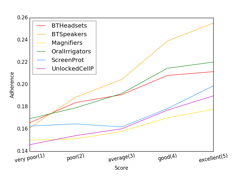
Amazon Dataset. For each product category, we extract the reference terminology, by considering all the reviews belonging to that category against the contrastive dataset, for the appropriate language. Then, we compute the adherence value for each review. To show the results in a meaningful way, we grouped reviews in 5 bins, according to their score, and compute the average of the adherence values on each bin. The results are reported in Figure 2.

The graph shows a line for each product category. Overall, it highlights that reviews with higher scores have higher adherence, implying a better correspondence with the reference terminology in comparison to reviews with lower scores. This result could be biased by the fact that reviews with higher scores are more represented in the dataset than the others.

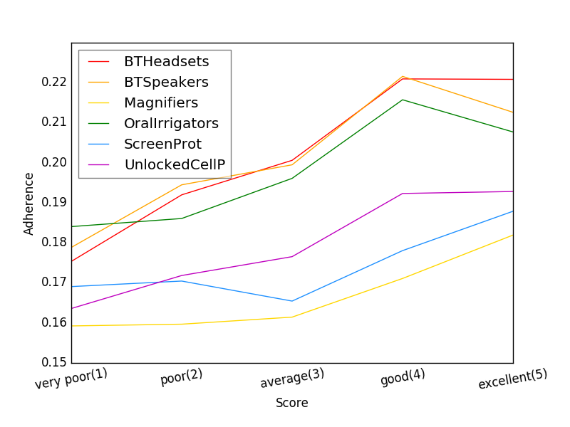
Therefore, we balanced the reviews in bins: we set $B$ as the number of reviews of the less populated bin and we randomly selected the same number of reviews from the other bins. Then, we recomputed the average adherence values and we obtained the results shown in Figure 2, which confirm the trend of the previous graph.

Even if the Bluetooth Speakers and Oral Irrigators categories feature a slight decreasing trend in the adherence value, when passing from reviews with score 4 to reviews with score 5, the general trend shows that the adherence metric is informative of the review score.

Figure 1: Score vs adherence - Amazon dataset - unbalanced.

Figure 2: Score vs adherence - Amazon dataset - balanced.

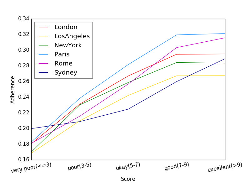
Booking Dataset. In the second experiment, we group the hotel reviews accordingly to the city they refer to. For each city, we extract the reference terminology and we compute the adherence value for each review. To make the results comparable with the ones obtained for Amazon  we re-arrange the Booking scoring system to generate a score evaluation over 5 bins. To this aim, we apply the score distribution suggested by Booking itself, since Booking scores are inflated to the top of the possible range of scores [16]. Therefore, we consider the following bin distribution:

• very poor: reviews with a score $\leq$ 3;

• poor: score $\in$ (3, 5];

• okay: score $\in$ (5, 7];

• good: score $\in$ (7, 9];

• excellent: score $>$ 9.

The results of the average adherence values on each bin are reported in Figure 4. A line is drawn for each city, by connecting the points in correspondence to the adherence values. The graph suggests that the average adherence is higher for reviews with higher scores. Thus, the higher the score of the hotel reviews, the more adherent the review to the reference terminology.

To avoid the bias caused by the over-representation of the positive reviews in the dataset, we compute the average adherence values by using a balanced number of reviews for each bin. The results, reported in Figure 4, confirm the trend of the previous graph, even if the slope is smaller.

Figure 3: Score vs adherence - Booking - unbalanced.

Figure 4: Score vs adherence - Booking - balanced.

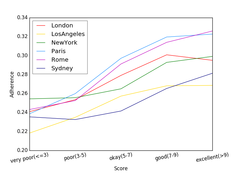
Working on balanced bins, the typical terminology of the reviews corpus has been recalculated, with respect to what computed for the original, unbalanced dataset. Thus, even considering the less populated bin, the average adherence value for the balanced dataset is not the same as the one in the unbalanced dataset for the same bin (this holds both for Booking and Amazon datasets).

The under-sampling applied to the majority classes to balance the reviews number leads to a deterioration of the results (both for Amazon and Booking - Figures 2 and 4.

4.2 Good Opinions, Higher Adherence

Interestingly, in the Booking dataset, the text of each review is conveniently divided into positive and negative content. Thus, we perform an additional experiment, by only considering positive and negative chunks of reviews. For each city, we group positive and negative contents of reviews and we compute the adherence value for each positive and negative chunk, with respect to the reference terminology. Finally, we average the adherence values according to the score bins. The results are reported in Figure 6, for the unbalanced dataset. In the graph, we report two lines for each city: the solid (dashed) lines are obtained by considering the positive (negative) contents of reviews. The same colour for solid and dashed line corresponds to the same city. We also perform the same calculation by considering a balanced dataset (Figure 6).

Figure 5: Score vs adherence - Booking unbalanced dataset - considering positive and negative contents separately.

Figure 6: Score vs adherence - Booking balanced dataset - considering positive and negative contents separately.

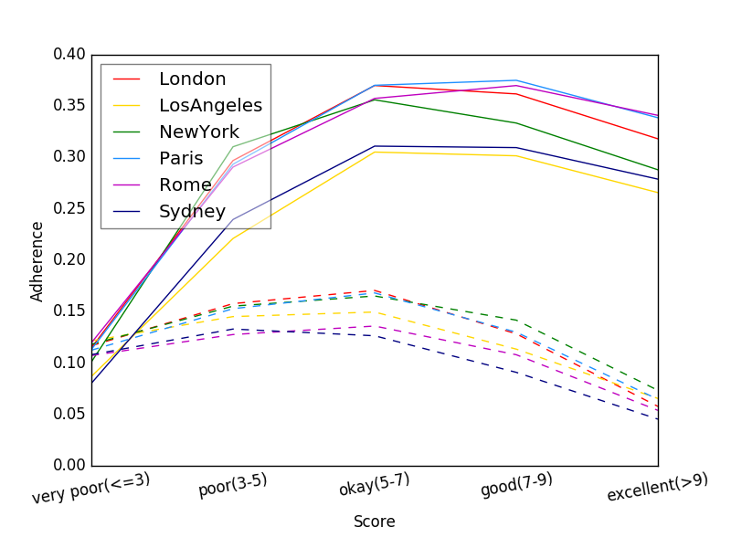
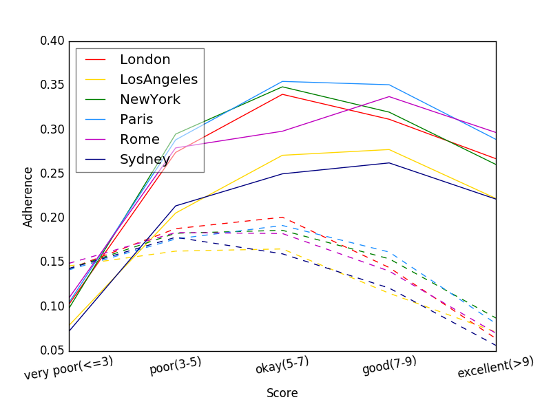
Both the graphs highlight that there is a clear division between the solid and dashed lines. In particular, the average adherence obtained considering positive contents is, for most of the bins, above the average adherence computed considering negative contents. This separation is more evident when the review score increases (it does not hold for very poor scores). Overall, positive aspects of a hotel are described with a less varied language with respect to its negative aspects. Probably, this phenomenon occurs because unsatisfied reviewers tend to explain what happened in details.

In addition to the average value, we also computed the standard deviation within each bin, that resulted to be quite high, as reported in Table 3, Table 4, Table 5 and Table 6. This suggests that, even correlated with the score, the adherence is not a good measure when considering a single review, but its informativeness should be rather exploited by considering an ensemble of reviews, as detailed in Section 4.4.

Table 3: Average adherence and the average standard deviation for six Amazon categories - unbalanced dataset.

	Bluetooth		Bluetooth		Magnifiers		Oral		Screen		Unlocked
	Headsets		Speakers				Irrigators		Protectors		CellPhones
Bin	Avg	Std	Avg	Std	Avg	Std	Avg	Std	Avg	Std	Avg	Std
1	0.17	0.07	0.16	0.08	0.15	0.08	0.17	0.07	0.16	0.07	0.15	0.06
2	0.18	0.07	0.19	0.07	0.15	0.07	0.18	0.07	0.16	0.07	0.15	0.06
3	0.19	0.07	0.20	0.08	0.16	0.08	0.19	0.07	0.16	0.07	0.16	0.07
4	0.21	0.08	0.24	0.09	0.17	0.08	0.21	0.08	0.18	0.08	0.18	0.08
5	0.21	0.09	0.26	0.11	0.18	0.09	0.22	0.08	0.20	0.09	0.19	0.10

Table 4: Average adherence and the average standard deviation for six Amazon categories - balanced dataset.

	Bluetooth		Bluetooth		Magnifiers		Oral		Screen		Unlocked
	Headsets		Speakers				Irrigators		Protectors		CellPhones
Bin	Avg	Std	Avg	Std	Avg	Std	Avg	Std	Avg	Std	Avg	Std
1	0.17	0.07	0.18	0.08	0.16	0.08	0.18	0.07	0.17	0.07	0.15	0.06
2	0.19	0.07	0.2	0.07	0.16	0.08	0.19	0.06	0.17	0.07	0.16	0.06
3	0.19	0.07	0.21	0.08	0.16	0.08	0.2	0.07	0.16	0.07	0.16	0.07
4	0.21	0.08	0.23	0.08	0.17	0.08	0.22	0.08	0.18	0.08	0.18	0.08
5	0.21	0.09	0.23	0.09	0.18	0.09	0.21	0.08	0.19	0.09	0.18	0.09

Table 5: Average adherence and the average standard deviation for six Booking cities - unbalanced dataset.

	London		LosAngeles		NewYork		Paris		Rome		Sydney
Bin	Avg	Std	Avg	Std	Avg	Std	Avg	Std	Avg	Std	Avg	Std
1	0.18	0.15	0.17	0.13	0.17	0.15	0.18	0.14	0.18	0.14	0.20	0.16
2	0.23	0.16	0.21	0.15	0.23	0.16	0.24	0.17	0.22	0.15	0.21	0.15
3	0.27	0.17	0.24	0.16	0.26	0.17	0.28	0.18	0.26	0.17	0.22	0.15
4	0.29	0.19	0.27	0.17	0.28	0.18	0.32	0.19	0.30	0.18	0.26	0.18
5	0.30	0.19	0.27	0.18	0.28	0.18	0.32	0.19	0.32	0.18	0.29	0.19

Table 6: Average adherence and the average standard deviation for six Booking cities - balanced dataset.

	London		LosAngeles		NewYork		Paris		Rome		Sydney
Bin	Avg	Std	Avg	Std	Avg	Std	Avg	Std	Avg	Std	Avg	Std
1	0.24	0.18	0.22	0.15	0.25	0.22	0.24	0.18	0.24	0.17	0.27	0.23
2	0.25	0.16	0.23	0.16	0.25	0.17	0.26	0.18	0.26	0.17	0.25	0.16
3	0.27	0.17	0.25	0.16	0.27	0.17	0.29	0.18	0.29	0.16	0.23	0.14
4	0.30	0.19	0.27	0.17	0.29	0.19	0.32	0.20	0.31	0.18	0.28	0.18
5	0.30	0.20	0.28	0.19	0.29	0.19	0.31	0.18	0.32	0.19	0.30	0.21

4.3 Extension to Different Languages

The experiments described so far were realised by considering a subset of reviews in English, taken from the original Booking dataset, which features other languages too. To further evaluate the informativness of the adherence metric, we selected two additional review subsets, in Italian and in French. For each subset, we drawn two graphs, the first considering all the reviews content, the second the separation between positive and negative contents. For these experiments, we considered imbalanced bins, due to the limited number of reviews available in each language. The results are reported in Figure 7.

(a) All content, Italian

(b) Positive/negative content, Italian

(c) All content, French

(d) Positive/negative content, French

Figure 7: Score vs adherence - Booking  unbalanced dataset - reviews in Italian and French.

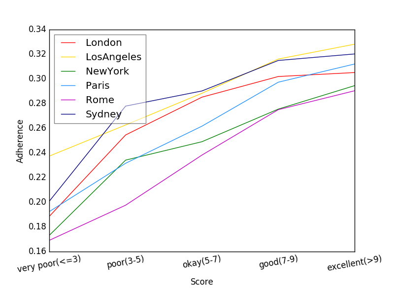
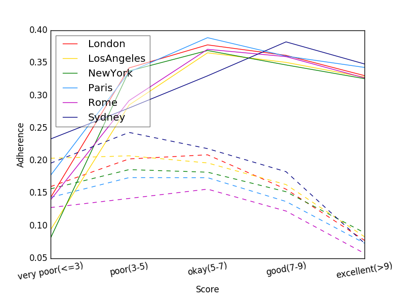
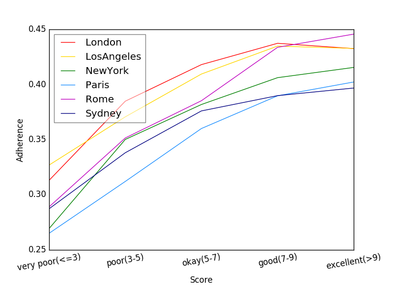
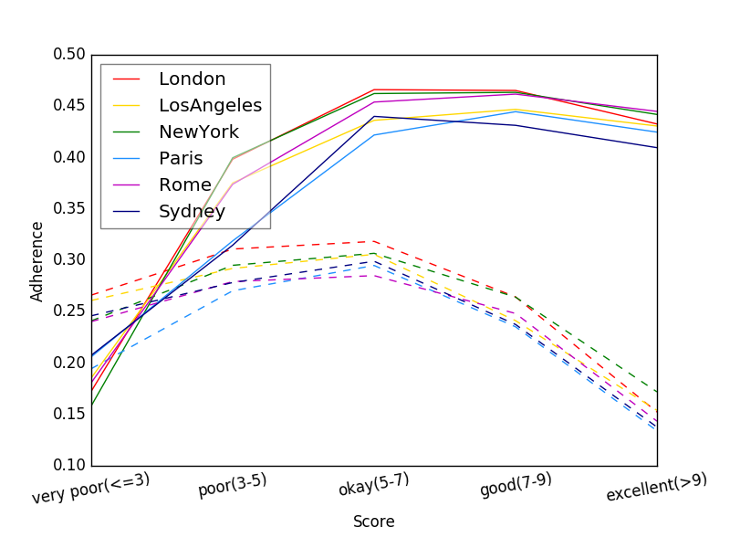
Essentially, in both cases, it is confirmed that the higher the score, the higher the adherence when considering the overall text (Figure 7-a and Figure 7-c). Similarily, the graphs in Figure 7-b and Figure 7-d show a clear division between positive and negative adherence values, when the score increases.

4.4 Language and Domain-Agnostic Reviews Aggregation

In this section, we present an application of the outcome found in previous ones. Given a set of texts, we propose to aggregate texts with positive polarity and texts with negative polarity, without a priori knowing the text language and domain, and without using any technique of Natural Language Processing (NLP), while exploiting only the adherence metric. We apply the following methodology:

1. For each review $r\in\mathcal{I}_{j}\in\mathcal{C}_{i}$ we compute the adherence $\text{adh}_{\mathbb{T}_{\mathcal{C}_{i}}}(r)$.

2. Reviews $r\in\mathcal{I}_{j}$ are sorted in ascending order w.r.t. their adherence value.

3. Ordered reviews are split in bins with the same cardinality. We defined $K_{\text{bins}}$ bins, each holding $|\{r\in\mathcal{I}_{j}\}|/K_{\text{bins}}$ reviews in ascending order of adherence.

4. For each bin $B_{i}$, we compute the average of the adherence value of the reviews it contains: $\text{Avg}_{\text{adh},i}=\frac{1}{R}\sum\text{adh}_{\mathbb{T}_{\mathcal{C}_{i}}}(r)$, as well as, for the purposes of validation, the average score provided by those reviews, $\text{Avg}_{\text{score},i}=\frac{1}{R}\sum\text{score}(r)$.

5. Finally, we aim at proving that, when the average adherence value of each bin increases, the average score value also increases. Thus, we compute the percentage of $\mathcal{I}_{j}\in\mathcal{C}_{i}$ for which we observe:

   $$\text{Avg}_{\text{score},K_{\text{bins}}}\geq\text{Avg}_{\text{score},1}$$ (5)

   $$\text{Avg}_{\text{score},i}\geq\text{Avg}_{\text{score},i-1}$$ (6)

   where $\text{Avg}_{\text{score},K_{\text{bins}}}$ is the average score for the last bin, $\text{Avg}_{\text{score},1}$ is the average score for the first bin, and $i=1,\dots,K_{\text{bins}}$.

Table 7 reports the results for the Amazon dataset. For each category $\mathcal{C}_{i}$, we apply the methodology three times, modifying the minimum number of reviews (minRev) for each item $\mathcal{I}_{j}$, in order to discard items with few reviews. We set $K_{\text{bins}}$=3 and we report the number of items (#$\mathcal{I}$) and the total number of reviews (#Rev) considered, plus the percentage of $\mathcal{I}_{j}\in\mathcal{C}_{i}$ for which (5) is true (%).

Table 7: Amazon dataset - parameters: equation (5), bins = 3.

Category $\mathcal{C}_{i}$	minRev=20			minRev=50			minRev=100
	#$\mathcal{I}_{j}$	#Rev	(%)	#$\mathcal{I}_{j}$	#Rev	(%)	#$\mathcal{I}_{j}$	#Rev	(%)
BluetoothHeadsets	817	108693	86	423	96393	93	223	82723	97
BluetoothSpeakers	82	13155	96	54	12278	100	27	10423	100
ScreenProtectors	1741	174320	83	781	144597	90	370	116337	96
UnlockedCellPhones	1116	97049	89	542	78836	94	257	58788	97
Magnifiers	143	8763	72	46	5714	87	18	3694	100
OralIrrigators	48	10301	85	32	9832	91	21	8987	90

This result shows that, considering 3 bins, the percentage of items for which the average score of the last bin is higher than the average score of the first bin is above 80% for each category (except for Magnifiers in case the minimum number of reviews is 20). Nevertheless, the percentage grows in almost all cases, when the minimum number of reviews increases. It exceeds 90% for every category, when the minimum number of reviews is, at least, 100.

Therefore, in the majority of cases, it is true that, when the average adherence of reviews belonging to the last bin is higher than the average adherence of reviews included in the first bin, the same relation exists between their correspondent average scores. This finding is mostly supported when we consider only items with many reviews (at least 100).

For the Booking dataset, we straight consider only hotels with at least 100 reviews. We perform three experiments according to the languages of reviews (English, Italian, and French). For each experiment, $K_{\text{bins}}$=3 and we report the number of items (#$\mathcal{I}$), the total number of reviews (#Rev) considered and the percentage of $\mathcal{I}_{j}\in\mathcal{C}_{i}$ for which (5) is true (%). The results are in Table 8. The percentage of items for which the average score of the last bin is higher than the average score of the first bin is above 90% in all the cases.

Table 8: Booking dataset considering different languages - parameters: equation (5), bins = 3. Not enough Italian reviews were available for Los Angeles and Sydney.

Category $\mathcal{C}_{i}$	English			Italian			French
	#$\mathcal{I}_{j}$	#Rev	(%)	#$\mathcal{I}_{j}$	#Rev	(%)	#$\mathcal{I}_{j}$	#Rev	(%)
London	356	467863	97	76	11952	96	123	20507	94
LosAngeles	56	46700	93	-	-	-	7	993	100
NewYork	163	182438	95	27	6518	93	60	10753	90
Paris	211	93164	96	6	806	100	72	12623	90
Rome	144	68543	97	64	11040	94	28	4197	93
Sydney	74	126744	100	-	-	-	4	553	100

Thus, given a set of reviews on, e.g., hotels, or restaurants, in any language, we can identify a group of reviews that, on average, express better opinions than another group of reviews. Noticeably, this analysis works even if the associated score is not available, i.e., it can be applied to general comments about items.

We consider now if also relation (6) is verified for each bin $i=1,\dots,K_{\text{bins}}$, i.e., if the function between the ordered sets of average adherence values $\text{Avg}_{\text{adh},i}$ and average score values $\text{Avg}_{score,i}$ is a monotonic function. By plotting the average score vs the average adherence, for some items, we found out a general upward trend. Nevertheless, there were many spikes that prevent the function from being monotonic. Then, we tried to smooth down the curves by applying a moving average with $window=2$ and we then computed the percentage of $\mathcal{I}_{j}\in\mathcal{C}_{i}$ for which (6) was verified. For the Amazon dataset, we performed three experiments, modifying the minimum number of reviews required (minRev) for each item, in order to discard items with few reviews. Results are in Table 9.

Table 9: Amazon dataset - parameters: equation (6), bins = 3.

Category $\mathcal{C}_{i}$	minRev=20 (%)	minRev=50 (%)	minRev=100 (%)
BluetoothHeadsets	69	76	82
BluetoothSpeakers	88	93	96
UnlockedCellPhones	69	72	77
Magnifiers	58	72	72
OralIrrigators	77	81	76
ScreenProtectors	58	66	73

Such results are worse with respect to the ones in Table 7. Nevertheless, in all cases (but Oral Irrigators), the percentage values increase when $minRev$ increase (for Magnifiers, it remains the same with $minRev=50,100$). When $minRev=100$, the percentage of $\mathcal{I}_{j}\in\mathcal{C}_{i}$ for which (6) is true is above 72%.

For the Booking dataset, due to the high number of available reviews, we also varied the number of bins from 3 to 5. We only considered reviews in English and computed the percentage of items for which the equation (6) is true. Table 10 shows a clear degradation of performances when the number of bin increases.

Table 10: Booking dataset - parameters: equation (6).

Category $\mathcal{C}_{i}$	bins=3 (%)	bins=4 (%)	bins=5 (%)
London	95	83	67
LosAngeles	88	75	61
New York	88	66	47
Paris	87	65	40
Rome	94	82	67
Sydney	95	92	85

So far, the results indicate a relation between the increasing adherence values and the increasing score values. However, we cannot prove a strong correlation between adherence and score, either considering a single review or groups of reviews. Therefore, we followed a different approach, by computing, for each item $\mathcal{I}_{j}\in\mathcal{C}_{i}$, the difference between the average values of the first and last bin, both for the adherence and the score:

$$\Delta_{\text{adh}}(j)=\text{Avg}_{\text{adh},K_{\text{bins}}}-\text{Avg}_{\text{adh},1}$$

$$\Delta_{\text{score}}(j)=\text{Avg}_{\text{score},K_{\text{bins}}}-\text{Avg}_{\text{score},1}$$

If we average such differences for all the items $\mathcal{I}_{j}\in\mathcal{C}_{i}$, both for adherence and score, we obtain an average value for each category $\mathcal{C}_{i}$:

$$\text{AvgD}_{\text{adh}}=\frac{1}{J}\sum_{j=1}^{J}\Delta_{\text{adh}}(j)$$ (7)

$$\text{AvgD}_{\text{score}}=\frac{1}{J}\sum_{j=1}^{J}\Delta_{\text{score}}(j)$$ (8)

where $J$ is the total number of items $j\in\mathcal{I}_{j}$.

(a) Bluetooth headsets

(b) Bluetooth speakers

(c) London (en)

(d) New York (en)

Figure 8: Average differences for Amazon and Booking example categories.

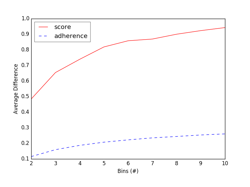
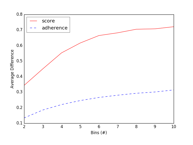
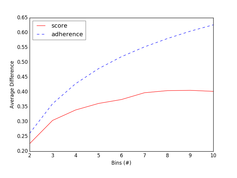
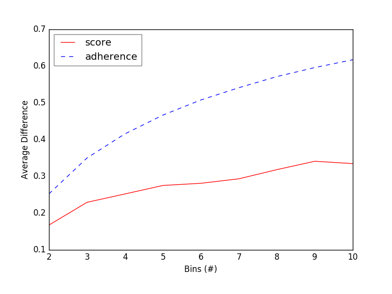
Figure 8 shows the values of (7) and (8) for items belonging to some of the Amazon and Booking categories. In each graph, the x-axis reports the number of bins considered, wheres the y-axis represents the average differences values. We depicted the average differences for the adherence with a solid red line, while the average differences for the score with a dashed blue line. The graphs clearly show that, when the number of bin increases, the first and last bin include reviews which describe the product in a considerably different way, in term of positiveness. Thus, given a category, it is possible to discriminate among groups of reviews, related to that category, in such a way that each group expresses an opinion different from the others, ordered from the most negative to the most positive ones (or vice-versa).

4.5 Representative Terms in First and Last Bins

Here, we extract the most recurrent terms in the positive and negative groups of reviews. Given an item (either a hotel or a product), we consider the terms included in the positive set and in the negative set (last and first bins, with $K_{\text{bins}}=10$) that can be also found in the extracted terminology.

For each term, we compute the term frequency–inverse document frequency (tf-idf) value (in this case, tf is the term frequency inside the bin, that is the number of reviews that include such term), we sort the terms accordingly and we select the first 20 ones for the positive and negative set. We then remove the terms common to both sets, in order to identify the most discriminating ones. Table 11 shows the terms extracted for two Amazon products.

Table 11: The most relevant positive and negative terms for two Amazon products.

Product	Negative		Positive
	Terms	Score	Terms	Score
B005XA0DNQ	refund, packaging, casing, disconnected, gift, battery, packaged, addition, hooked, plugging, shipping, 99, hook, speaker, purpose, sounds, kitchen	2.9	compact, sound, great, retractable, portable, very, price, unbelievable, satisfied, product, easy, recommend, small, perfect, little, handy, size	4.3
B0083RXA86	stereo, impressive, mostly, charger, button, product, charging, switch, louder, useless, price, usb	2.4	blue, charge, useful, very, coating, satisfied, quite, battery, enough, music, attachment, excellent, highly, quality, pleased	4.6

Table 12: The most relevant positive and negative terms for the Amazon categories.

Product	Negative terms	Positive terms
BluetoothHeadsets	charge, item, amazon, hear, purchased, device, problem, bought	fit, clear, recommend, highly, music, easy, excellent, comfortable, quality
BluetoothSpeakers	reviews, speakers, gift, charge, volume, item, amazon, music, purchased, charging, bought	little, portable, excellent, bluetooth, easy, recommend, small, sounds, highly, quality, size
ScreenProtectors	purchase, cover, bought, item, iphone, pack, instructions	perfect, samsung, clear, highly, fits, apply, perfectly
UnlockedCellPhones	buy, phone, phones, seller, cell, everything, amazon, iphone, item, problem, bought	perfect, excellent, fast, card, easy, recommend, android, quality, sim
AppetiteControl	try, tried, these, hungry, pills, reviews, products, oz, bottle, waste, eat, bought	loss, cambogia, lost, pounds, garcinia, recommend, diet, highly, definitely, lose, extract, exercise

After having extracted the terms for every item, we calculate their frequency within a whole category. Again, we remove the terms common to both sets (positive and negative), to highlight the most representative positive and negative terms for the category. Table 12 shows the terms extracted for the five Amazon categories with more reviews. Table 13 shows the terms extracted for some Booking categories, for English, Italian and French. However, for Italian and French, few examples are shown, due to the low number of reviews for such datasets.

Table 13: The most relevant positive and negative terms for Booking categories.

City	Negative terms	Positive terms
London (en)	booked, bar, floor, wifi, stayed, stay, shower, receptionist, reception, booking, hotels	helpful, cleanliness, convenient, quiet, comfortable, beds, facilities, clean, excellent, friendly, size
New York (en)	booked, square, checked, floor, door, stayed, stay, reception, desk, reservation, booking, hotels	perfect, bathroom, helpful, cleanliness, comfortable, beds, clean, excellent, small, noisy, friendly, size
Rome (it)	albergo, prenotazione, servizi, stanze, hotel, struttura, soggiorno, reception, doccia, booking	disponibile, cortesia, gentile, confortevole, termini, ottima, gentilezza, abbondante, pulita, cordiale
Paris (fr)	emplacement, gare, accueil, anglais, chambres, hotel, clients, avons, sol, londres, wifi, lit, chambre, réservation, hôtel, réception, payé, bruit, booking	salle, géographique, déjeuner, proche, confortable, petite, petit, qualité, quartier, très, métro, calme, propreté, literie, situation, propre, agréable, proximité, bain

5 Related Work

Terminology extraction.

Automatic terminology extraction is one of the pillars of many terminology engineering processes, such as text mining, information retrieval, ontology learning, and semantic web technologies. The aim is to automatically identify relevant concepts (or terms) from a given domain-specific corpus. Within a collection of candidate domain-relevant terms, actual terms are separated from non-terms by using statistical and machine learning methods [20]. Here, we rely on contrastive approaches, where the identification of relevant candidates is performed through inter-domain contrastive analysis [21, 6, 1].

Opinion Mining.

Opinion mining techniques aim at automatically identifying polarities and sentiments in texts[11], by, e.g., extracting subjective expressions representing personal opinions and speculations[25] or detecting so called contextual polarity of a word, i.e., the polarity acquired by the word contextually to the sentence in which it appears, see, e.g., [26, 27, 17]. Often, opinion mining rely on lexicon-based approaches, involving the extraction of term polarities from sentiment lexicons and the aggregation of such scores to predict the overall sentiment of a piece of text, see, e.g., [5, 8, 4, 3].

Clustering Opinions.

Unsupervised learning does not require labelled data for the training process. Among them, clustering algorithms can be profitably used to find the natural clusters in the data, by calculating the distances or similarities from the centres of the clusters. Few efforts have been devoted to the study of polarity detection in online reviews with clustering techniques. In [9], the authors present the clustering-based sentiment analysis approach, by applying three different techniques, namely TF-IDF weighting, voting mechanism and enhancement by hybrid with scoring method. In [13, 12], the authors describe and experimental study of some common clustering techniques used for sentiment analysis of online reviews and investigate how any step of the clustering process (pre-processing, term weighting, clustering algorithm) can affect clustering results. The work in [18] studies the relationship between online movie reviews and the box office incomes. The detection of sentiments is carried out by using tf and idf values as features and Fuzzy Clustering as algorithm.

Here, we proposed an alternative approach to polarity detection, relying on automatic terminology extraction, in a domain and language agnostic fashion, and not relying on linguistic resources.

6 Final Remarks

We presented a novel approach for aggregating reviews, based on their polarity. The methodology did not require pre-labeled reviews and the knowledge of the reviews’ domain and language. We introduced the adherence metric and we demonstrated its correlation with the review score. Lastly, we relied on adherence to successfully aggregate reviews, according to the opinions they express.

References

- [1] Basili, R., et al.: A contrastive approach to term extraction. In: Terminologie et intelligence artificielle. Rencontres. pp. 119–128 (2001)
- [2] Bonin, F., et al.: A contrastive approach to multi-word extraction from domain-specific corpora. In: Language Resources and Evaluation. ELRA (2010)
- [3] Bravo-Marquez, F., et al.: Building a twitter opinion lexicon from automatically-annotated tweets. Knowledge-Based Systems 108, 65–78 (2016)
- [4] Cambria, E., Hussain, A.: Sentic Computing: A Common-Sense-Based Framework for Concept-Level Sentiment Analysis. Springer (2015)
- [5] Cambria, E., et al.: SenticNet 3: a common and common-sense knowledge base for cognition-driven sentiment analysis. In: 28th AAAI Artificial Intelligence. pp. 1515–1521 (2014)
- [6] Chung, T.M., Nation, P.: Identifying technical vocabulary. System 32(2), 251–263 (2004)
- [7] Del Vigna, F., Petrocchi, M., Tommasi, A., Zavattari, C., Tesconi, M.: Semi-supervised knowledge extraction for detection of drugs and their effects. In: Social Informatics I (2016)
- [8] Esuli, A., Sebastiani, F.: SENTIWORDNET: A publicly available lexical resource for opinion mining. In: Language Resources and Evaluation. pp. 417–422 (2006)
- [9] Li, G., Liu, F.: Application of a clustering method on sentiment analysis. J. Inf. Sci. 38(2), 127–139 (2012)
- [10] Ling Lo, S., et al.: A multilingual semi-supervised approach in deriving Singlish sentic patterns for polarity detection. Knowledge-Based Systems 105, 236–247 (2016)
- [11] Liu, B.: Sentiment Analysis and Opinion Mining. Morgan & Claypool (2012)
- [12] Ma, B., Yuan, H., Wu, Y.: Exploring performance of clustering methods on document sentiment analysis. Information Science (2015)
- [13] Ma, B., et al.: A comparison study of clustering models for online review sentiment analysis. In: Web-Age Information Management. pp. 332–337. Springer (2013)
- [14] McAuley, J., Pandey, R., Leskovec, J.: Inferring networks of substitutable and complementary products. In: 21th KDD. pp. 785–794. ACM (2015)
- [15] McAuley, J., et al.: Image-based recommendations on styles and substitutes. In: 38th Research and Development in Information Retrieval. pp. 43–52. ACM (2015)
- [16] Mellinas, J.P., María-Dolores, S.M.M., García, J.J.B.: Booking.com: The unexpected scoring system. Tourism Management 49, 72–74 (2015)
- [17] Muhammad, A., Wiratunga, N., Lothian, R.: Contextual sentiment analysis for social media genres. Knowledge-Based Systems 108, 92–101 (2016)
- [18] Nagamma, P., et al.: An improved sentiment analysis of online movie reviews based on clustering for box-office prediction. In: Computing, Communication and Automation. pp. 933–937 (2015)
- [19] Pang, B., Lee, L.: Opinion mining and sentiment analysis. Found. Trends Inf. Retr. 2(1-2), 1–135 (2008)
- [20] Pazienza, M.T., et al.: Terminology extraction: An analysis of linguistic and statistical approaches. In: Knowledge Mining, pp. 255–279. Springer (2005)
- [21] Peñas, A., Verdejo, F., Gonzalo, J.: Corpus-based terminology extraction applied to information access. In: Corpus Linguistics. vol. 13, pp. 458–465 (2001)
- [22] Ren, Y., Zhang, Y., Zhang, M., Ji, D.: Context-sensitive Twitter sentiment classification using neural network. In: Artificial Intelligence. pp. 215–221. AAAI (2016)
- [23] Salton, G., Buckley, C.: Term-weighting approaches in automatic text retrieval. Inf. Process. Management 24(5), 513–523 (1988)
- [24] Turney, P.D.: Thumbs up or thumbs down?: Semantic orientation applied to unsupervised classification of reviews. In: Computational Linguistics Meeting. pp. 417–424. ACL (2002)
- [25] Wilson, T., et al.: OpinionFinder: A system for subjectivity analysis. In: HLT/EMNLP on Interactive Demonstrations. pp. 34–35. ACL (2005)
- [26] Wilson, T., et al.: Recognizing contextual polarity in phrase-level sentiment analysis. In: HLT/EMNLP. pp. 347–354. ACL (2005)
- [27] Wilson, T., et al.: Recognizing contextual polarity: An exploration of features for phrase-level sentiment analysis. Comput. Linguist. 35(3), 399–433 (2009)