ad2]Krishnan SRINIVASARENGAN ad2]José RAGOT ad2]Christophe AUBRUN ad2]Didier MAQUIN \correspondingauthorKrishnan SRINIVASARENGAN

An adaptive observer design approach for discrete-time nonlinear systems

[    [    [    [ CRAN UMR 7039, Université de Lorraine, Vandoeuvre-lès-Nancy, Cedex, France CRAN UMR 7039, CNRS, France
e-mail: (krishnan.srinivasarengan,jose.ragot,christophe.aubrun,didier.maquin)@univ-lorraine.fr
Abstract

We discuss a design approach for nonlinear discrete-time adaptive observer. This involves transforming a nonlinear system into a quasi-LPV (Linear Parameter Varying) polytopic model in Takagi-Sugeno (T-S) form using nonlinear embedding and sector nonlinearity (SNL) transformation. We then develop a discrete-time counterpart for a joint state and parameter estimation, based on design strategies developed for continuous time models in the existing literature. The design uses a Lyapunov approach and provides an error bounded by 𝕃2subscript𝕃2\mathbb{L}_{2} gain. Based on this strategy, we propose a design for adaptive observers for nonlinear systems whose T-S form can have unmeasured premise variables.

keywords:
Adaptive observer, Joint state and parameter estimation, Takagi-Sugeno model, time-varying parameter estimation, Sector nonlinearity transformation.

1 Introduction

The term adaptive observers is used to represent joint state and parameter observers that estimate the states and parameters independently without augmenting them with the states [ticlea_adaptive_2016]. For nonlinear systems, a systematic procedure for adaptive observers was first proposed in [cho_systematic_1997]. These results were characterized further in [besancon_remarks_2000], where an adaptive observer form was introduced. However, the extension to discrete-time systems is not straightforward as it exploits the particular structure arising in continuous-time trajectories.

Other systematic adaptive observer design procedures attempt at specific applications such as fault diagnosis. In [caccavale2008adaptive], a diagnostic observer with an adaptive uncertainties estimation component is provided. All the states are assumed measured allowing the authors to use an innovation term as 𝐞x,k+1(AKo)𝐞x,ksubscript𝐞𝑥𝑘1𝐴subscript𝐾𝑜subscript𝐞𝑥𝑘\mathbf{e}_{x,k+1}-(A-K_{o})\mathbf{e}_{x,k}, where A𝐴A and Kosubscript𝐾𝑜K_{o} are the system and the state observer gain matrices respectively with 𝐞x,ksubscript𝐞𝑥𝑘\mathbf{e}_{x,k} representing the state error. This innovation allows for a cancellation of terms that complicate the adaptation of the approach in [cho_systematic_1997] to discrete-time. Another fault detection application based on the design of an adaptive observer is proposed in [thumati_model_2008]. Here, the model uncertainties are bounded by known constants and hence it was possible to propose a state observer with a Luenberger form. The parameter estimation component of the observer is tailored for fault detection using terms for fault detection such as threshold and dead-zone. The focus on fault detection allows these works to tune the observers with specific constraints, hence generalizing them to a generic adaptive observer is ruled out.

One way to develop observers for general nonlinear systems could be using equivalent forms. A recurring theme in the above works in boundedness of inputs, matrix entries, etc. If we add them with boundedness of the states of the system, we can obtain consider using the linear parameter varying (LPV) or quasi-LPV system formulations. A nonlinear state equation of the form,

𝐱k+1=f(𝐱k,𝐮k)subscript𝐱𝑘1𝑓subscript𝐱𝑘subscript𝐮𝑘\displaystyle\mathbf{x}_{k+1}=f(\mathbf{x}_{k},\mathbf{u}_{k}) (1)

could be put through a systematic procedure of factorizing them like that proposed in [kwiatkowski_automated_2006] to obtain a quasi-LPV form as,

𝐱k+1=A(𝐱k,𝐮k)𝐱k+B(𝐱k,𝐮k)𝐮ksubscript𝐱𝑘1𝐴subscript𝐱𝑘subscript𝐮𝑘subscript𝐱𝑘𝐵subscript𝐱𝑘subscript𝐮𝑘subscript𝐮𝑘\displaystyle\mathbf{x}_{k+1}=A(\mathbf{x}_{k},\mathbf{u}_{k})\mathbf{x}_{k}+B(\mathbf{x}_{k},\mathbf{u}_{k})\mathbf{u}_{k} (2)

For a system with unknown parameters θjsubscript𝜃𝑗\theta_{j} in the adaptive observer form of [cho_systematic_1997], the quasi-LPV form would be,

𝐱k+1=j=1nθ(Aj(𝐱k,𝐮k)𝐱kθj+Bj(𝐱k,𝐮k)𝐮kθj)subscript𝐱𝑘1superscriptsubscript𝑗1subscript𝑛𝜃subscript𝐴𝑗subscript𝐱𝑘subscript𝐮𝑘subscript𝐱𝑘subscript𝜃𝑗subscript𝐵𝑗subscript𝐱𝑘subscript𝐮𝑘subscript𝐮𝑘subscript𝜃𝑗\displaystyle\mathbf{x}_{k+1}=\sum_{j=1}^{n_{\theta}}\left(A_{j}(\mathbf{x}_{k},\mathbf{u}_{k})\mathbf{x}_{k}\theta_{j}+B_{j}(\mathbf{x}_{k},\mathbf{u}_{k})\mathbf{u}_{k}\theta_{j}\right) (3)

and possibly with an affine term. Here, nθsubscript𝑛𝜃n_{\theta} is the number of parameters. The observer design strategy for such quasi-LPV systems could follow that of the linear time-varying (LTV) systems, if the matrices depend only on measured variables like outputs and inputs, as pointed out in [ticlea_exponential_2013].

In that direction, we can consider the adaptive observer proposed for LTV systems in [guyader2003adaptive], which takes inspiration from its continuous-time counterpart in [zhang2002adaptive]. The authors propose an innovation term whose gain is obtained by filtering the parameters’ transmission matrix in the state equation. This structure along with some boundedness assumption allow showing the exponential convergence of the observer. If the system has bounded zero mean noise, the estimation errors have an expected value that exponentially converges to zero. The main issue with this approach is the lack of clear procedure to choose a scalar that helps to guarantee convergence. These criticisms lead the authors in [ticlea_adaptive_2016] to propose an exponential forgetting factor based approach adopted from [ticlea_exponential_2013]. This approach mimics a Kalman filter with an update and propagation step, but has two interconnected exponential forgetting factor designs, thus preserving the adaptive observer structure. The main assumptions are complete uniform observability of the system and the invertibility of the system matrix of the LTV, Ak,ksubscript𝐴𝑘for-all𝑘A_{k},\ \forall k.

The LTV based observers, however, cannot handle the case when the system matrices depend on one of the unmeasured states. This type of design can be handled in the realm of one of the quasi-LPV polytopic models: Takagi-Sugeno (T-S) form. One way to obtain a T-S model, that exactly represents the original nonlinear system with a sector, is using the sector nonlinearity (SNL) transformation [ohtake2003fuzzy]. For the quasi-LPV model in (3), applying SNL would lead to a T-S model of the form,

𝐱k+1subscript𝐱𝑘1\displaystyle\mathbf{x}_{k+1} =i=12npμi(𝐳k)[(Ai+j=1nθA¯ijθj)𝐱k\displaystyle=\sum_{i=1}^{2^{n_{p}}}\mu_{i}(\mathbf{z}_{k})\left[(A_{i}+\sum_{j=1}^{n_{\theta}}\bar{A}_{ij}\theta_{j})\mathbf{x}_{k}\right.
+(Bi+j=1nθB¯ijθj))𝐮k]\displaystyle\left.\qquad\qquad\qquad\qquad+(B_{i}+\sum_{j=1}^{n_{\theta}}\bar{B}_{ij}\theta_{j}))\mathbf{u}_{k}\right]
𝐲ksubscript𝐲𝑘\displaystyle\mathbf{y}_{k} =C𝐱kabsent𝐶subscript𝐱𝑘\displaystyle=C\mathbf{x}_{k} (4)

where, npsubscript𝑛𝑝n_{p} is the number of premise variables 𝐳ksubscript𝐳𝑘\mathbf{z}_{k}, which could be one of the states, inputs, and outputs. We consider a linear output equation, as in [cho_systematic_1997]. We assert that the observer design for such models can cover all possible systems that are represented by those in [cho_systematic_1997]. The observer for this type of system should take into account the fact that the weighting functions μisubscript𝜇𝑖\mu_{i} would be depending on estimated premise variables, rather than exact ones. Fortunately, there is a growing body of literature for observer design for T-S system with unmeasured premise variables [lendek2010stability], as well as using immersion techniques to avoid T-S systems with unmeasured premise variables [ichalal2016method].

In this paper, we first develop a method for joint state and time-varying parameter estimation. The approach springs from the idea in [bezzaoucha2013state2] to represent a time-varying parameter using SNL transformation. This was extended to T-S models with time-varying parameters in [bezzaoucha2013state]. We derived the discrete-time version for the T-S models in [srinivasarengan:hal-01399791]. In the present paper, we derive the time-varying parameter estimation for a linear system to illustrate the equivalence with that for the T-S models in [srinivasarengan:hal-01399791]. With this design approach, we propose an adaptive observer design for nonlinear systems whose T-S form has unmeasured premise variables. This would fill the gap that is left in the nonlinear discrete-time adaptive observers that cannot be solved by adapting LTV based design approaches.

This work builds on top of our communication in [srinivasarengan:hal-01399791]. The key improvements are: to show the generalized nature of the results for both LTV and T-S system, providing extensions and refinement through corollaries, and to propose an adaptive observer design using the joint state and time-varying parameter estimation approach. Further, the illustration involves a different, but a more relevant example. The outline of the paper is as follows: the following section discusses the preliminaries that are used later in the paper. The Sec. 3 discusses the model structure idea and formulates the problem. The joint state and time-varying parameter are derived for a linear time-varying system in Sec.4. These results are customized to design an adaptive observer design for nonlinear discrete-time systems in Sec. 5. A simulation example is given in Sec. 6 to illustrate the proposed method. The paper is then summarized with a future outlook in Sec. 7.

2 Preliminaries

2.1 Notations

Takagi-Sugeno models [tanaka2004fuzzy] are of the form,

𝐱k+1subscript𝐱𝑘1\displaystyle\mathbf{x}_{k+1} =i=1rμi(𝐳k)[Ai𝐱k+Bi𝐮k]absentsuperscriptsubscript𝑖1𝑟subscript𝜇𝑖subscript𝐳𝑘delimited-[]subscript𝐴𝑖subscript𝐱𝑘subscript𝐵𝑖subscript𝐮𝑘\displaystyle=\sum_{i=1}^{r}\mu_{i}(\mathbf{z}_{k})\left[A_{i}\mathbf{x}_{k}+B_{i}\mathbf{u}_{k}\right]
𝐲ksubscript𝐲𝑘\displaystyle\mathbf{y}_{k} =C𝐱kabsent𝐶subscript𝐱𝑘\displaystyle=C\mathbf{x}_{k} (5)

Here, r=2np𝑟superscript2subscript𝑛𝑝r=2^{n_{p}}, where npsubscript𝑛𝑝n_{p} is the number of premise variables 𝐳ksubscript𝐳𝑘\mathbf{z}_{k}. The weighting functions μi(𝐳k)subscript𝜇𝑖subscript𝐳𝑘\mu_{i}(\mathbf{z}_{k}) capture the nonlinearity associated with the corresponding premise variables. Further,

𝐱knx,𝐮knu,𝐳knp,𝐲knyformulae-sequencesubscript𝐱𝑘superscriptsubscript𝑛𝑥formulae-sequencesubscript𝐮𝑘superscriptsubscript𝑛𝑢formulae-sequencesubscript𝐳𝑘superscriptsubscript𝑛𝑝subscript𝐲𝑘superscriptsubscript𝑛𝑦\displaystyle\mathbf{x}_{k}\in\mathbb{R}^{n_{x}},\ \mathbf{u}_{k}\in\mathbb{R}^{n_{u}},\ \mathbf{z}_{k}\in\mathbb{R}^{n_{p}},\ \mathbf{y}_{k}\in\mathbb{R}^{n_{y}}

and

Ainx×nx,Binx×nu,Cny×nx,iformulae-sequencesubscript𝐴𝑖superscriptsubscript𝑛𝑥subscript𝑛𝑥formulae-sequencesubscript𝐵𝑖superscriptsubscript𝑛𝑥subscript𝑛𝑢𝐶superscriptsubscript𝑛𝑦subscript𝑛𝑥for-all𝑖\displaystyle A_{i}\in\mathbb{R}^{n_{x}\times n_{x}},\ \ B_{i}\in\mathbb{R}^{n_{x}\times n_{u}},\ \ C\in\mathbb{R}^{n_{y}\times n_{x}},\forall i (6)

Given a symmetric matrix,

A=[a11a12a22]𝐴matrixsubscript𝑎11subscript𝑎12subscript𝑎22\displaystyle A=\begin{bmatrix}a_{11}&a_{12}\\ *&a_{22}\end{bmatrix}

the ’*’ symbol represents the symmetric transpose element, that is, in this case, =a12T*=a_{12}^{T}.

2.2 Preliminary Results

The following known results would be referred to while proving the results in this work,

Lemma 2.1.

[boyd1994linear] For a symmetric matrix M𝑀M, given by,

M=[ABBTC]𝑀matrix𝐴𝐵superscript𝐵𝑇𝐶\displaystyle M=\begin{bmatrix}A&B\\ B^{T}&C\end{bmatrix}

if C𝐶C is invertible, then the following properties hold:

  1. 1.

    M>0𝑀0M>0 iff C>0andABC1BT>0𝐶0𝑎𝑛𝑑𝐴𝐵superscript𝐶1superscript𝐵𝑇0C>0\ and\ A-BC^{-1}B^{T}>0

  2. 2.

    if C>0𝐶0C>0, then M0𝑀0M\geq 0 iff ABC1BT0𝐴𝐵superscript𝐶1superscript𝐵𝑇0A-BC^{-1}B^{T}\geq 0.

Lemma 2.2.

[zhou1988robust] Consider two matrices X𝑋X and Y𝑌Y with appropriate dimensions, a time-varying matrix ΔksubscriptΔ𝑘\Delta_{k} and a positive scalar λ𝜆\lambda. The following property is verified:

XTΔkTY+YTΔkXλXTX+λ1YTYsuperscript𝑋𝑇subscriptsuperscriptΔ𝑇𝑘𝑌superscript𝑌𝑇subscriptΔ𝑘𝑋𝜆superscript𝑋𝑇𝑋superscript𝜆1superscript𝑌𝑇𝑌\displaystyle X^{T}\Delta^{T}_{k}Y+Y^{T}\Delta_{k}X\leq\lambda X^{T}X+\lambda^{-1}Y^{T}Y (7)

for ΔkTΔkIsubscriptsuperscriptΔ𝑇𝑘subscriptΔ𝑘𝐼\Delta^{T}_{k}\Delta_{k}\leq I

Lemma 2.3.

[de1992discrete] For a discrete-time system of the form,

𝐱k+1subscript𝐱𝑘1\displaystyle\mathbf{x}_{k+1} =A𝐱k+B𝐮kabsent𝐴subscript𝐱𝑘𝐵subscript𝐮𝑘\displaystyle=A\mathbf{x}_{k}+B\mathbf{u}_{k}
𝐲ksubscript𝐲𝑘\displaystyle\mathbf{y}_{k} =C𝐱k+D𝐮kabsent𝐶subscript𝐱𝑘𝐷subscript𝐮𝑘\displaystyle=C\mathbf{x}_{k}+D\mathbf{u}_{k} (8)

the Bounded Real Lemma equivalent LMI condition for stability is,

P=PT>0,𝑃superscript𝑃𝑇0\displaystyle\qquad\qquad P=P^{T}>0,
[ATPAP+CTCATPB+CTDBTPA+DTCDTD+BTPBΓ2]0matrixsuperscript𝐴𝑇𝑃𝐴𝑃superscript𝐶𝑇𝐶superscript𝐴𝑇𝑃𝐵superscript𝐶𝑇𝐷superscript𝐵𝑇𝑃𝐴superscript𝐷𝑇𝐶superscript𝐷𝑇𝐷superscript𝐵𝑇𝑃𝐵subscriptΓ20\displaystyle\begin{bmatrix}A^{T}PA-P+C^{T}C&A^{T}PB+C^{T}D\\ B^{T}PA+D^{T}C&D^{T}D+B^{T}PB-\Gamma_{2}\end{bmatrix}\leq 0

where Γ2subscriptΓ2\Gamma_{2} is the 𝕃2subscript𝕃2\mathbb{L}_{2} gain between the input 𝐮ksubscript𝐮𝑘\mathbf{u}_{k} and the output 𝐲ksubscript𝐲𝑘\mathbf{y}_{k}.

3 System Model and Problem Formulation

3.1 Representing a time-varying parameter using SNL

The idea of the estimation of time-varying parameter lies in representing it using the sector nonlinearity (SNL) transformation. The SNL assumes that the parameter is bounded and its boundary values are known. For a scalar parameter θk[θ1,θ2]subscript𝜃𝑘superscript𝜃1superscript𝜃2\theta_{k}\in[\theta^{1},\theta^{2}], we could write,

θk=μ1(θk)θ1+μ2(θk)θ2subscript𝜃𝑘superscript𝜇1subscript𝜃𝑘superscript𝜃1superscript𝜇2subscript𝜃𝑘superscript𝜃2\displaystyle\theta_{k}=\mu^{1}(\theta_{k})\theta^{1}+\mu^{2}(\theta_{k})\theta^{2} (9)

where,

μ1(θk)=θ2θkθ2θ1,μ2(θk)=θkθ1θ2θ1formulae-sequencesuperscript𝜇1subscript𝜃𝑘superscript𝜃2subscript𝜃𝑘superscript𝜃2superscript𝜃1superscript𝜇2subscript𝜃𝑘subscript𝜃𝑘superscript𝜃1superscript𝜃2superscript𝜃1\displaystyle\mu^{1}(\theta_{k})=\frac{\theta^{2}-\theta_{k}}{\theta^{2}-\theta^{1}},\qquad\mu^{2}(\theta_{k})=\frac{\theta_{k}-\theta^{1}}{\theta^{2}-\theta^{1}} (10)

The membership functions satisfy the convex sum property, that is,

iμi(.)=1,0μi(.)1,i\displaystyle\sum_{i}\mu^{i}(.)=1,\qquad 0\leq\mu^{i}(.)\leq 1,\ \forall i (11)

Hence each parameter could be represented by a weighted sum of two elements.

Remark 3.1.

For a vector case, or for T-S systems with unknown parameters, the membership functions can be manipulated to obtain weighting functions that depend on the same variables. To illustrate this, take the case of two unknown parameters, θ1,k[θ11,θ12]subscript𝜃1𝑘superscriptsubscript𝜃11superscriptsubscript𝜃12\theta_{1,k}\in[\theta_{1}^{1},\theta_{1}^{2}] and θ2,k[θ21,θ22]subscript𝜃2𝑘superscriptsubscript𝜃21superscriptsubscript𝜃22\theta_{2,k}\in[\theta_{2}^{1},\theta_{2}^{2}] and represented as,

θ1,ksubscript𝜃1𝑘\displaystyle\theta_{1,k} =μ11(θ1,k)θ11+μ12(θ1,k)θ12absentsuperscriptsubscript𝜇11subscript𝜃1𝑘superscriptsubscript𝜃11superscriptsubscript𝜇12subscript𝜃1𝑘superscriptsubscript𝜃12\displaystyle=\mu_{1}^{1}(\theta_{1,k})\theta_{1}^{1}+\mu_{1}^{2}(\theta_{1,k})\theta_{1}^{2}
θ2,ksubscript𝜃2𝑘\displaystyle\theta_{2,k} =μ21(θ2,k)θ21+μ22(θ2,k)θ22absentsuperscriptsubscript𝜇21subscript𝜃2𝑘superscriptsubscript𝜃21superscriptsubscript𝜇22subscript𝜃2𝑘superscriptsubscript𝜃22\displaystyle=\mu_{2}^{1}(\theta_{2,k})\theta_{2}^{1}+\mu_{2}^{2}(\theta_{2,k})\theta_{2}^{2} (12)

We can now create a new formulation for the unknown parameters by,

θ1,ksubscript𝜃1𝑘\displaystyle\theta_{1,k} =(μ21(θ2,k)+μ22(θ2,k))θ1,kabsentsuperscriptsubscript𝜇21subscript𝜃2𝑘superscriptsubscript𝜇22subscript𝜃2𝑘subscript𝜃1𝑘\displaystyle=\left(\mu_{2}^{1}(\theta_{2,k})+\mu_{2}^{2}(\theta_{2,k})\right)\theta_{1,k}
θ2,ksubscript𝜃2𝑘\displaystyle\theta_{2,k} =(μ11(θ1,k)+μ12(θ1,k))θ2,kabsentsuperscriptsubscript𝜇11subscript𝜃1𝑘superscriptsubscript𝜇12subscript𝜃1𝑘subscript𝜃2𝑘\displaystyle=(\mu_{1}^{1}(\theta_{1,k})+\mu_{1}^{2}(\theta_{1,k}))\theta_{2,k} (13)

By bringing the alternative form in (12), we obtain the variables that depend on the same, but 4 weighting functions, which are the products of the membership functions of the original representation. In general, this approach would lead to 2nθsuperscript2subscript𝑛𝜃2^{n_{\theta}} submodels, where nθsubscript𝑛𝜃n_{\theta} is the number of parameters. A detailed treatment of this representation could be obtained from [nagy2010systematic].

3.2 System Model Structures

Consider a linear time-varying system, the time varying nature is due to the unknown parameters ΘksubscriptΘ𝑘\Theta_{k} as follows:

𝐱k+1subscript𝐱𝑘1\displaystyle\mathbf{x}_{k+1} =A(Θk)𝐱k+B(Θk)𝐮kabsent𝐴subscriptΘ𝑘subscript𝐱𝑘𝐵subscriptΘ𝑘subscript𝐮𝑘\displaystyle=A(\Theta_{k})\mathbf{x}_{k}+B(\Theta_{k})\mathbf{u}_{k}
𝐲ksubscript𝐲𝑘\displaystyle\mathbf{y}_{k} =C𝐱kabsent𝐶subscript𝐱𝑘\displaystyle=C\mathbf{x}_{k} (14)

where ΘknθsubscriptΘ𝑘superscriptsubscript𝑛𝜃\Theta_{k}\in\mathbb{R}^{n_{\theta}} is used to represent the vector of θi,i1,..,nθ\theta_{i},\forall i\in 1,..,n_{\theta}. We consider only a specific form of time-varying matrices that takes the following form:

A(Θk)𝐴subscriptΘ𝑘\displaystyle A(\Theta_{k}) =A0+i=1nθθi,kA¯i,absentsubscript𝐴0superscriptsubscript𝑖1subscript𝑛𝜃subscript𝜃𝑖𝑘subscript¯𝐴𝑖\displaystyle=A_{0}+\sum_{i=1}^{n_{\theta}}\theta_{i,k}\bar{A}_{i},
B(Θk)𝐵subscriptΘ𝑘\displaystyle B(\Theta_{k}) =B0+i=1nθθi,kB¯iabsentsubscript𝐵0superscriptsubscript𝑖1subscript𝑛𝜃subscript𝜃𝑖𝑘subscript¯𝐵𝑖\displaystyle=B_{0}+\sum_{i=1}^{n_{\theta}}\theta_{i,k}\bar{B}_{i} (15)

that is, it is possible to write the time-varying matrix as a sum of constant matrices that are scaled by the unknown parameter. We can use the SNL transformation as in (9), to represent the matrices of time-varying parameters. Let us consider a scalar case,

A(θk)𝐴subscript𝜃𝑘\displaystyle A(\theta_{k}) =A0+θkA¯absentsubscript𝐴0subscript𝜃𝑘¯𝐴\displaystyle=A_{0}+\theta_{k}\bar{A}
=A0+(μ1(θk)θ1+μ2(θk)θ2)A¯absentsubscript𝐴0superscript𝜇1subscript𝜃𝑘superscript𝜃1superscript𝜇2subscript𝜃𝑘superscript𝜃2¯𝐴\displaystyle=A_{0}+(\mu^{1}(\theta_{k})\theta^{1}+\mu^{2}(\theta_{k})\theta^{2})\bar{A}
=j=12μj(θk)(A0+θj)A¯absentsuperscriptsubscript𝑗12superscript𝜇𝑗subscript𝜃𝑘subscript𝐴0superscript𝜃𝑗¯𝐴\displaystyle=\sum_{j=1}^{2}\mu^{j}(\theta_{k})(A_{0}+\theta^{j})\bar{A} (16)

with θjsuperscript𝜃𝑗\theta^{j} corresponding to one of θ1superscript𝜃1\theta^{1} or θ2superscript𝜃2\theta^{2} depending upon the submodel j𝑗j. Similarly,

B(θk)𝐵subscript𝜃𝑘\displaystyle B(\theta_{k}) =j=12μj(θk)(B0+θj)B¯absentsuperscriptsubscript𝑗12superscript𝜇𝑗subscript𝜃𝑘subscript𝐵0superscript𝜃𝑗¯𝐵\displaystyle=\sum_{j=1}^{2}\mu^{j}(\theta_{k})(B_{0}+\theta^{j})\bar{B} (17)

This could then be extended to the vector case to yield,

A(Θk)𝐴subscriptΘ𝑘\displaystyle A(\Theta_{k}) =i=1rhi(Θk)(A0+θiA¯i),absentsuperscriptsubscript𝑖1𝑟subscript𝑖subscriptΘ𝑘subscript𝐴0superscript𝜃𝑖subscript¯𝐴𝑖\displaystyle=\sum_{i=1}^{r}h_{i}(\Theta_{k})(A_{0}+\theta^{i}\bar{A}_{i}),
B(Θk)𝐵subscriptΘ𝑘\displaystyle B(\Theta_{k}) =i=1rhi(Θk)(B0+θiB¯i)absentsuperscriptsubscript𝑖1𝑟subscript𝑖subscriptΘ𝑘subscript𝐵0superscript𝜃𝑖subscript¯𝐵𝑖\displaystyle=\sum_{i=1}^{r}h_{i}(\Theta_{k})(B_{0}+\theta^{i}\bar{B}_{i}) (18)

where r=2nθ𝑟superscript2subscript𝑛𝜃r=2^{n_{\theta}}. Here hi(Θk)subscript𝑖subscriptΘ𝑘h_{i}(\Theta_{k}) is the normalized product of a membership function μij(θi,k)superscriptsubscript𝜇𝑖𝑗subscript𝜃𝑖𝑘\mu_{i}^{j}(\theta_{i,k}) of each parameter corresponding the submodel i𝑖i (See Remark 3.1) and θisuperscript𝜃𝑖\theta^{i} represents the sector boundary values of each parameter corresponding to the submodel i𝑖i. More details could be obtained from [tanaka2004fuzzy]. This would lead to

𝐱k+1subscript𝐱𝑘1\displaystyle\mathbf{x}_{k+1} =i=1rhi(Θk)(Ai𝐱k+Bi𝐮k)absentsuperscriptsubscript𝑖1𝑟subscript𝑖subscriptΘ𝑘subscript𝐴𝑖subscript𝐱𝑘subscript𝐵𝑖subscript𝐮𝑘\displaystyle=\sum_{i=1}^{r}h_{i}(\Theta_{k})(A_{i}\mathbf{x}_{k}+B_{i}\mathbf{u}_{k})
𝐲ksubscript𝐲𝑘\displaystyle\mathbf{y}_{k} =C𝐱kabsent𝐶subscript𝐱𝑘\displaystyle=C\mathbf{x}_{k} (19)

with

Aisubscript𝐴𝑖\displaystyle A_{i} =A0+j=1nθθjiA¯iBi=B0+j=1nθθjiB¯iformulae-sequenceabsentsubscript𝐴0superscriptsubscript𝑗1subscript𝑛𝜃superscriptsubscript𝜃𝑗𝑖subscript¯𝐴𝑖subscript𝐵𝑖subscript𝐵0superscriptsubscript𝑗1subscript𝑛𝜃superscriptsubscript𝜃𝑗𝑖subscript¯𝐵𝑖\displaystyle=A_{0}+\sum_{j=1}^{n_{\theta}}\theta_{j}^{i}\bar{A}_{i}\qquad B_{i}=B_{0}+\sum_{j=1}^{n_{\theta}}\theta_{j}^{i}\bar{B}_{i} (20)

where θjisuperscriptsubscript𝜃𝑗𝑖\theta_{j}^{i} is the corresponding maximum or minimum value of θjsubscript𝜃𝑗\theta_{j} for the submodel i𝑖i. For the model in (19), we propose an observer of the form,

𝐱^k+1subscript^𝐱𝑘1\displaystyle\mathbf{\hat{x}}_{k+1} =i=1rhi(Θ^k)(Ai𝐱^k+Bi𝐮k+Li(𝐲k𝐲^k))absentsuperscriptsubscript𝑖1𝑟subscript𝑖subscript^Θ𝑘subscript𝐴𝑖subscript^𝐱𝑘subscript𝐵𝑖subscript𝐮𝑘subscript𝐿𝑖subscript𝐲𝑘subscript^𝐲𝑘\displaystyle=\sum_{i=1}^{r}h_{i}(\hat{\Theta}_{k})(A_{i}\mathbf{\hat{x}}_{k}+B_{i}\mathbf{u}_{k}+L_{i}(\mathbf{y}_{k}-\mathbf{\hat{y}}_{k}))
Θ^k+1subscript^Θ𝑘1\displaystyle\hat{\Theta}_{k+1} =Θ^k+i=1rhi(Θ^k)(Ky,i(𝐲k𝐲^k)KθΘ^k)absentsubscript^Θ𝑘superscriptsubscript𝑖1𝑟subscript𝑖subscript^Θ𝑘subscript𝐾𝑦𝑖subscript𝐲𝑘subscript^𝐲𝑘subscript𝐾𝜃subscript^Θ𝑘\displaystyle=\hat{\Theta}_{k}+\sum_{i=1}^{r}h_{i}(\hat{\Theta}_{k})(K_{y,i}(\mathbf{y}_{k}-\mathbf{\hat{y}}_{k})-K_{\theta}\hat{\Theta}_{k})
𝐲^ksubscript^𝐲𝑘\displaystyle\mathbf{\hat{y}}_{k} =Cx^kabsent𝐶subscript^𝑥𝑘\displaystyle=C\hat{x}_{k} (21)

The gains Linx×nysubscript𝐿𝑖superscriptsubscript𝑛𝑥subscript𝑛𝑦L_{i}\in\mathbb{R}^{n_{x}\times n_{y}} and Ky,inθ×nysubscript𝐾𝑦𝑖superscriptsubscript𝑛𝜃subscript𝑛𝑦K_{y,i}\in\mathbb{R}^{n_{\theta}\times n_{y}} are to be estimated while the gain Kθnθ×nθsubscript𝐾𝜃superscriptsubscript𝑛𝜃subscript𝑛𝜃K_{\theta}\in\mathbb{R}^{n_{\theta}\times n_{\theta}} is chosen. The choice of Kθsubscript𝐾𝜃K_{\theta} shall typically be in the form of a diagonal matrix. In the initial work [bezzaoucha2013state], this was introduced to avoid a marginal stability condition for the error dynamics. As discussed in [srinivasarengan2016nonlinear], choosing this reduces the number of variables in the final LMI to solve and hence allows for a computationally tractable problem. Further, in the discrete-time case, Kθsubscript𝐾𝜃K_{\theta} as a variable leads to unresolvable nonlinear terms in the matrix inequalities.

3.3 Uncertain-like model representation

Let us define the state estimation error 𝐞𝐱,k=𝐱k𝐱^ksubscript𝐞𝐱𝑘subscript𝐱𝑘subscript^𝐱𝑘\mathbf{e}_{\mathbf{x},k}=\mathbf{x}_{k}-\mathbf{\hat{x}}_{k}. If we want to analyse the dynamics of the errors based on the system and observer models in (19) and (21), it would involve comparing systems weighted by functions that depend on mismatched variables (i.e., 𝐱k,Θksubscript𝐱𝑘subscriptΘ𝑘\mathbf{x}_{k},\Theta_{k} vs 𝐱^k,Θ^ksubscript^𝐱𝑘subscript^Θ𝑘\mathbf{\hat{x}}_{k},\hat{\Theta}_{k}). This is a typical problem in observer design for T-S systems with unmeasured premise variables. There are different approaches to deal with it. In this work, we use the approach proposed in [ichalal2009state] to develop an uncertain-like model representation. By making use of the convex sum property in (11), we can rewrite (19), without making any approximations, as,

𝐱k+1subscript𝐱𝑘1\displaystyle\mathbf{x}_{k+1} =i=1rhi(Θ^k)(Ai𝐱k+Bi𝐮k)absentsuperscriptsubscript𝑖1𝑟subscript𝑖subscript^Θ𝑘subscript𝐴𝑖subscript𝐱𝑘subscript𝐵𝑖subscript𝐮𝑘\displaystyle=\sum_{i=1}^{r}h_{i}(\hat{\Theta}_{k})(A_{i}\mathbf{x}_{k}+B_{i}\mathbf{u}_{k})
+i=1r(hi(Θk)hi(Θ^k))(Ai𝐱k+Bi𝐮k)superscriptsubscript𝑖1𝑟subscript𝑖subscriptΘ𝑘subscript𝑖subscript^Θ𝑘subscript𝐴𝑖subscript𝐱𝑘subscript𝐵𝑖subscript𝐮𝑘\displaystyle\qquad+\sum_{i=1}^{r}(h_{i}(\Theta_{k})-h_{i}(\hat{\Theta}_{k}))(A_{i}\mathbf{x}_{k}+B_{i}\mathbf{u}_{k})
𝐲ksubscript𝐲𝑘\displaystyle\mathbf{y}_{k} =C𝐱kabsent𝐶subscript𝐱𝑘\displaystyle=C\mathbf{x}_{k} (22)

Let us denote,

ΔAkΔsubscript𝐴𝑘\displaystyle\Delta A_{k} =i=1r(hi(Θk)hi(Θ^k))Ai=𝒜ΣA,kEAabsentsuperscriptsubscript𝑖1𝑟subscript𝑖subscriptΘ𝑘subscript𝑖subscript^Θ𝑘subscript𝐴𝑖𝒜subscriptΣ𝐴𝑘subscript𝐸𝐴\displaystyle=\sum_{i=1}^{r}(h_{i}(\Theta_{k})-h_{i}(\hat{\Theta}_{k}))A_{i}=\mathcal{A}\Sigma_{A,k}E_{A}
ΔBkΔsubscript𝐵𝑘\displaystyle\Delta B_{k} =i=1r(hi(Θk)hi(Θ^k))Bi=ΣB,kEBabsentsuperscriptsubscript𝑖1𝑟subscript𝑖subscriptΘ𝑘subscript𝑖subscript^Θ𝑘subscript𝐵𝑖subscriptΣ𝐵𝑘subscript𝐸𝐵\displaystyle=\sum_{i=1}^{r}(h_{i}(\Theta_{k})-h_{i}(\hat{\Theta}_{k}))B_{i}=\mathcal{B}\Sigma_{B,k}E_{B} (23)

where,

𝒜𝒜\displaystyle\mathcal{A} =[A1A2Ar]nx×nxrabsentmatrixsubscript𝐴1subscript𝐴2subscript𝐴𝑟superscriptsubscript𝑛𝑥subscript𝑛𝑥𝑟\displaystyle=\begin{bmatrix}A_{1}&A_{2}&...&A_{r}\end{bmatrix}\in\mathbb{R}^{n_{x}\times n_{x}r}
EAsubscript𝐸𝐴\displaystyle E_{A} =[InxInxInx]Tnxr×nxabsentsuperscriptmatrixsubscript𝐼subscript𝑛𝑥subscript𝐼subscript𝑛𝑥subscript𝐼subscript𝑛𝑥𝑇superscriptsubscript𝑛𝑥𝑟subscript𝑛𝑥\displaystyle=\begin{bmatrix}I_{n_{x}}&I_{n_{x}}&...&I_{n_{x}}\end{bmatrix}^{T}\in\mathbb{R}^{n_{x}r\times n_{x}}
ΣA,ksubscriptΣ𝐴𝑘\displaystyle\Sigma_{A,k} =[(h1h^1)Inx00(hrh^r)Inx]absentmatrixsubscript1subscript^1subscript𝐼subscript𝑛𝑥missing-subexpressionmissing-subexpression0missing-subexpressionmissing-subexpressionmissing-subexpression0missing-subexpressionmissing-subexpressionsubscript𝑟subscript^𝑟subscript𝐼subscript𝑛𝑥\displaystyle=\begin{bmatrix}(h_{1}-\hat{h}_{1})I_{n_{x}}&&&\makebox(0.0,0.0)[]{\text{\Large 0}}\\ &&\cdots&\\ \makebox(0.0,0.0)[]{\text{\Large 0}}&&&(h_{r}-\hat{h}_{r})I_{n_{x}}\\ \end{bmatrix} (24)

Similarly,

\displaystyle\mathcal{B} =[B1B2Br]nu×nurabsentmatrixsubscript𝐵1subscript𝐵2subscript𝐵𝑟superscriptsubscript𝑛𝑢subscript𝑛𝑢𝑟\displaystyle=\begin{bmatrix}B_{1}&B_{2}&...&B_{r}\end{bmatrix}\in\mathbb{R}^{n_{u}\times n_{u}r}
EBsubscript𝐸𝐵\displaystyle E_{B} =[InuInuInu]Tnur×nuabsentsuperscriptmatrixsubscript𝐼subscript𝑛𝑢subscript𝐼subscript𝑛𝑢subscript𝐼subscript𝑛𝑢𝑇superscriptsubscript𝑛𝑢𝑟subscript𝑛𝑢\displaystyle=\begin{bmatrix}I_{n_{u}}&I_{n_{u}}&...&I_{n_{u}}\end{bmatrix}^{T}\in\mathbb{R}^{n_{u}r\times n_{u}}
ΣB,ksubscriptΣ𝐵𝑘\displaystyle\Sigma_{B,k} =[(h1h^1)Inu00(hrh^r)Inu]absentmatrixsubscript1subscript^1subscript𝐼subscript𝑛𝑢missing-subexpressionmissing-subexpression0missing-subexpressionmissing-subexpressionmissing-subexpression0missing-subexpressionmissing-subexpressionsubscript𝑟subscript^𝑟subscript𝐼subscript𝑛𝑢\displaystyle=\begin{bmatrix}(h_{1}-\hat{h}_{1})I_{n_{u}}&&&\makebox(0.0,0.0)[]{\text{\Large 0}}\\ &&\cdots&\\ \makebox(0.0,0.0)[]{\text{\Large 0}}&&&(h_{r}-\hat{h}_{r})I_{n_{u}}\\ \end{bmatrix} (25)

with hisubscript𝑖h_{i} and h^isubscript^𝑖\hat{h}_{i} stand for hi(Θ)subscript𝑖Θh_{i}(\Theta) and h^i(Θ)subscript^𝑖Θ\hat{h}_{i}(\Theta) respectively. Noting that 1(hih^i)11subscript𝑖subscript^𝑖1-1\leq(h_{i}-\hat{h}_{i})\leq 1, the matrices ΣA,knxr×nxrsubscriptΣ𝐴𝑘superscriptsubscript𝑛𝑥𝑟subscript𝑛𝑥𝑟\Sigma_{A,k}\in\mathbb{R}^{n_{x}r\times n_{x}r}, ΣB,knur×nursubscriptΣ𝐵𝑘superscriptsubscript𝑛𝑢𝑟subscript𝑛𝑢𝑟\Sigma_{B,k}\in\mathbb{R}^{n_{u}r\times n_{u}r} have the useful property,

ΣA,kTΣA,kI,ΣB,kTΣB,kIformulae-sequencesuperscriptsubscriptΣ𝐴𝑘𝑇subscriptΣ𝐴𝑘𝐼superscriptsubscriptΣ𝐵𝑘𝑇subscriptΣ𝐵𝑘𝐼\displaystyle\Sigma_{A,k}^{T}\Sigma_{A,k}\leq I,\qquad\Sigma_{B,k}^{T}\Sigma_{B,k}\leq I (26)

which will later be used to bound the time-varying difference between the known and estimated weighting functions. This will lead to the system model (19) be represented as,

𝐱k+1subscript𝐱𝑘1\displaystyle\mathbf{x}_{k+1} =i=1rhi(Θ^)[(Ai+ΔAk)𝐱k+(Bi+ΔBk)𝐮k]absentsuperscriptsubscript𝑖1𝑟subscript𝑖^Θdelimited-[]subscript𝐴𝑖Δsubscript𝐴𝑘subscript𝐱𝑘subscript𝐵𝑖Δsubscript𝐵𝑘subscript𝐮𝑘\displaystyle=\sum_{i=1}^{r}h_{i}(\hat{\Theta})[(A_{i}+\Delta A_{k})\mathbf{x}_{k}+(B_{i}+\Delta B_{k})\mathbf{u}_{k}]
𝐲ksubscript𝐲𝑘\displaystyle\mathbf{y}_{k} =C𝐱kabsent𝐶subscript𝐱𝑘\displaystyle=C\mathbf{x}_{k} (27)

As the model (27) and its observer (21) now share the same weighting functions hi(Θ^)subscript𝑖^Θh_{i}(\hat{\Theta}), it’s therefore possible to express in a more simple and tractable form the state and the parameter estimation errors.

4 Joint state and time-varying parameter estimation

In this section, we provide the results for the stability analysis of the design of joint state and parameter observer. The results can be considered the discrete-time version of the observer design in [bezzaoucha2013state] and follows the steps in [srinivasarengan:hal-01399791].

Theorem 4.1.

Given the system model of the form (19), there exists an observer of the form (21), if there exists P0subscript𝑃0P_{0}, P1subscript𝑃1P_{1}, Risubscript𝑅𝑖R_{i}, Fisubscript𝐹𝑖F_{i}, λ1subscript𝜆1\lambda_{1}, λ2subscript𝜆2\lambda_{2}, λ3subscript𝜆3\lambda_{3}, λ4subscript𝜆4\lambda_{4}, Γ2jsuperscriptsubscriptΓ2𝑗\Gamma_{2}^{j} (i[1,r],j{x,u,θ,Δθ}formulae-sequencefor-all𝑖1𝑟for-all𝑗𝑥𝑢𝜃Δ𝜃\forall i\in[1,r],\forall j\in\{x,u,\theta,\Delta\theta\}), such that,

P0=P0T>0,P1=P1T>0formulae-sequencesubscript𝑃0superscriptsubscript𝑃0𝑇0subscript𝑃1superscriptsubscript𝑃1𝑇0\displaystyle P_{0}=P_{0}^{T}>0,\ P_{1}=P_{1}^{T}>0
λm>0,m{1,2,3,4},Γ2j>0,jformulae-sequencesubscript𝜆𝑚0formulae-sequencefor-all𝑚1234superscriptsubscriptΓ2𝑗0for-all𝑗\displaystyle\lambda_{m}>0,\ \forall m\in\{1,2,3,4\},\ \Gamma_{2}^{j}>0,\forall j (28)
[P+IQA,iΦiTP0T220QBTT𝒜P0P*Λ]<0matrix𝑃𝐼subscript𝑄𝐴𝑖superscriptsubscriptΦ𝑖𝑇𝑃0missing-subexpressionsubscript𝑇220superscriptsubscript𝑄𝐵𝑇subscript𝑇𝒜𝑃0missing-subexpression𝑃missing-subexpressionmissing-subexpression*missing-subexpressionmissing-subexpressionΛ0\displaystyle\begin{bmatrix}-P+I&Q_{A,i}&\Phi_{i}^{T}P&0&\\ *&T_{22}&0&Q_{B}^{T}&T_{\mathcal{A}\mathcal{B}}\\ *&*&-P&0&\\ *&*&*&-P&\\ &\makebox(0.0,0.0)[]{\text{\Large*}}&&&\Lambda\\ \end{bmatrix}<0 (29)

Here,

P0,isubscript𝑃0𝑖\displaystyle P_{0,i} =AiTP0CTRiT,P=diag(P0,P1),formulae-sequenceabsentsuperscriptsubscript𝐴𝑖𝑇subscript𝑃0superscript𝐶𝑇superscriptsubscript𝑅𝑖𝑇𝑃𝑑𝑖𝑎𝑔subscript𝑃0subscript𝑃1\displaystyle=A_{i}^{T}P_{0}-C^{T}R_{i}^{T},\ \ P=diag(P_{0},P_{1}),
ΦiTPsuperscriptsubscriptΦ𝑖𝑇𝑃\displaystyle\Phi_{i}^{T}P =[P0,iCTFiT0KθTP1]absentmatrixsubscript𝑃0𝑖superscript𝐶𝑇subscriptsuperscript𝐹𝑇𝑖0superscriptsubscript𝐾𝜃𝑇subscript𝑃1\displaystyle=\begin{bmatrix}P_{0,i}&-C^{T}F^{T}_{i}\\ 0&-K_{\theta}^{T}P_{1}\end{bmatrix}
QA,isubscript𝑄𝐴𝑖\displaystyle Q_{A,i} =[00CTFiT(I+Kθ)CTFiT00KθTP1(I+Kθ)KθTP1]absentmatrix00superscript𝐶𝑇superscriptsubscript𝐹𝑖𝑇𝐼subscript𝐾𝜃superscript𝐶𝑇superscriptsubscript𝐹𝑖𝑇missing-subexpressionmissing-subexpressionmissing-subexpressionmissing-subexpressionmissing-subexpression00superscriptsubscript𝐾𝜃𝑇subscript𝑃1𝐼subscript𝐾𝜃superscriptsubscript𝐾𝜃𝑇subscript𝑃1\displaystyle=\begin{bmatrix}0&0&-C^{T}F_{i}^{T}(I+K_{\theta})&-C^{T}F_{i}^{T}\\ &&&&\\ 0&0&-K_{\theta}^{T}P_{1}(I+K_{\theta})&-K_{\theta}^{T}P_{1}\end{bmatrix}
QBsubscript𝑄𝐵\displaystyle Q_{B} =[00000(I+Kθ)TP10P1]absentmatrix00000superscript𝐼subscript𝐾𝜃𝑇subscript𝑃10subscript𝑃1\displaystyle=\begin{bmatrix}0&0\\ 0&0\\ 0&(I+K_{\theta})^{T}P_{1}\\ 0&P_{1}\end{bmatrix}
T22subscript𝑇22\displaystyle T_{22} =[T22110000T22220000Γ2θ0000Γ2Δθ]absentmatrixsuperscriptsubscript𝑇22110000superscriptsubscript𝑇22220000superscriptsubscriptΓ2𝜃0000superscriptsubscriptΓ2Δ𝜃\displaystyle=\begin{bmatrix}T_{22}^{11}&0&0&0\\ 0&T_{22}^{22}&0&0\\ 0&0&-\Gamma_{2}^{\theta}&0\\ 0&0&0&-\Gamma_{2}^{\Delta\theta}\end{bmatrix}
ΛΛ\displaystyle\Lambda =diag(λ1I,λ3I,λ2I,λ4I)absent𝑑𝑖𝑎𝑔subscript𝜆1𝐼subscript𝜆3𝐼subscript𝜆2𝐼subscript𝜆4𝐼\displaystyle=diag(-\lambda_{1}I,-\lambda_{3}I,-\lambda_{2}I,-\lambda_{4}I)
T𝒜subscript𝑇𝒜\displaystyle T_{\mathcal{A}\mathcal{B}} =[P0,i𝒜P0,i000000000000P0𝒜P0]absentmatrixsubscript𝑃0𝑖𝒜subscript𝑃0𝑖000000000000subscript𝑃0𝒜subscript𝑃0\displaystyle=\begin{bmatrix}P_{0,i}\mathcal{A}&P_{0,i}\mathcal{B}&0&0\\ 0&0&0&0\\ 0&0&0&0\\ 0&0&P_{0}\mathcal{A}&P_{0}\mathcal{B}\end{bmatrix} (30)

where, T2211=Γ2x+(λ1+λ2)EATEAsuperscriptsubscript𝑇2211superscriptsubscriptΓ2𝑥subscript𝜆1subscript𝜆2superscriptsubscript𝐸𝐴𝑇subscript𝐸𝐴T_{22}^{11}=-\Gamma_{2}^{x}+(\lambda_{1}+\lambda_{2})E_{A}^{T}E_{A} and T2222=Γ2u+(λ3+λ4)EBTEBsuperscriptsubscript𝑇2222superscriptsubscriptΓ2𝑢subscript𝜆3subscript𝜆4superscriptsubscript𝐸𝐵𝑇subscript𝐸𝐵T_{22}^{22}=-\Gamma_{2}^{u}+(\lambda_{3}+\lambda_{4})E_{B}^{T}E_{B}. The observer gains are given by,

Ky,i=P11Fi,Li=P01Riformulae-sequencesubscript𝐾𝑦𝑖superscriptsubscript𝑃11subscript𝐹𝑖subscript𝐿𝑖superscriptsubscript𝑃01subscript𝑅𝑖\displaystyle K_{y,i}=P_{1}^{-1}F_{i},\qquad L_{i}=P_{0}^{-1}R_{i} (31)
Proof 4.2.

Consider the uncertain-like representation of the system in (27). Comparing it with the observer (21), and defining errors of the form,

𝐞𝐱,k=𝐱k𝐱^k,𝐞Θ,k=ΘkΘ^kformulae-sequencesubscript𝐞𝐱𝑘subscript𝐱𝑘subscript^𝐱𝑘subscript𝐞Θ𝑘subscriptΘ𝑘subscript^Θ𝑘\displaystyle\mathbf{e}_{\mathbf{x},k}=\mathbf{x}_{k}-\mathbf{\hat{x}}_{k},\ \ \ \mathbf{e}_{\Theta,k}=\Theta_{k}-\hat{\Theta}_{k}

we get,

𝐞𝐱,k+1subscript𝐞𝐱𝑘1\displaystyle\mathbf{e}_{\mathbf{x},k+1} =i=1rhi(Θ^k)[(AiLiC)𝐞𝐱,k+ΔAk𝐱k+ΔBk𝐮k]absentsuperscriptsubscript𝑖1𝑟subscript𝑖subscript^Θ𝑘delimited-[]subscript𝐴𝑖subscript𝐿𝑖𝐶subscript𝐞𝐱𝑘Δsubscript𝐴𝑘subscript𝐱𝑘Δsubscript𝐵𝑘subscript𝐮𝑘\displaystyle=\sum_{i=1}^{r}h_{i}(\hat{\Theta}_{k})[(A_{i}-L_{i}C)\mathbf{e}_{\mathbf{x},k}+\Delta A_{k}\mathbf{x}_{k}+\Delta B_{k}\mathbf{u}_{k}]
𝐞Θ,k+1subscript𝐞Θ𝑘1\displaystyle\mathbf{e}_{\Theta,k+1} =i=1rhi(Θ^k)[ΔΘk+(I+Kθ)θk\displaystyle=\sum_{i=1}^{r}h_{i}(\hat{\Theta}_{k})[\Delta\Theta_{k}+(I+K_{\theta})\theta_{k}
Ky,iC𝐞𝐱,kKθ𝐞Θ,k]\displaystyle\qquad\qquad\qquad\qquad-K_{y,i}C\mathbf{e}_{\mathbf{x},k}-K_{\theta}\mathbf{e}_{\Theta,k}] (32)

where, ΔΘk=Θk+1ΘkΔsubscriptΘ𝑘subscriptΘ𝑘1subscriptΘ𝑘\Delta\Theta_{k}=\Theta_{k+1}-\Theta_{k}. We can represent this error dynamics as,

[𝐞𝐱,k+1𝐞Θ,k+1]=Φi[𝐞𝐱,k𝐞Θ,k]+Ψi,k[𝐱k𝐮kΘkΔΘk]matrixsubscript𝐞𝐱𝑘1missing-subexpressionsubscript𝐞Θ𝑘1subscriptΦ𝑖matrixsubscript𝐞𝐱𝑘missing-subexpressionsubscript𝐞Θ𝑘subscriptΨ𝑖𝑘matrixsubscript𝐱𝑘subscript𝐮𝑘subscriptΘ𝑘ΔsubscriptΘ𝑘\displaystyle\begin{bmatrix}\mathbf{e}_{\mathbf{x},k+1}\\ \\ \mathbf{e}_{\Theta,k+1}\end{bmatrix}=\Phi_{i}\begin{bmatrix}\mathbf{e}_{\mathbf{x},k}\\ \\ \mathbf{e}_{\Theta,k}\end{bmatrix}+\Psi_{i,k}\begin{bmatrix}\mathbf{x}_{k}\\ \mathbf{u}_{k}\\ \Theta_{k}\\ \Delta\Theta_{k}\end{bmatrix} (33)

where,

ΦisubscriptΦ𝑖\displaystyle\Phi_{i} =[AiLiC0Ky,iCKθ]absentmatrixsubscript𝐴𝑖subscript𝐿𝑖𝐶0subscript𝐾𝑦𝑖𝐶subscript𝐾𝜃\displaystyle=\begin{bmatrix}A_{i}-L_{i}C&0\\ -K_{y,i}C&-K_{\theta}\end{bmatrix}
Ψi,ksubscriptΨ𝑖𝑘\displaystyle\Psi_{i,k} =[ΔAkΔBk0000I+KθI]absentmatrixΔsubscript𝐴𝑘Δsubscript𝐵𝑘0000𝐼subscript𝐾𝜃𝐼\displaystyle=\begin{bmatrix}\Delta A_{k}&\Delta B_{k}&0&0\\ 0&0&I+K_{\theta}&I\end{bmatrix} (34)

Considering,

𝐞a,k=[𝐞𝐱,kT𝐞Θ,kT]T,u~k=[𝐱kT𝐮kTΘkTΔΘkT]Tformulae-sequencesubscript𝐞𝑎𝑘superscriptmatrixsuperscriptsubscript𝐞𝐱𝑘𝑇superscriptsubscript𝐞Θ𝑘𝑇𝑇subscript~𝑢𝑘superscriptmatrixsuperscriptsubscript𝐱𝑘𝑇superscriptsubscript𝐮𝑘𝑇superscriptsubscriptΘ𝑘𝑇ΔsuperscriptsubscriptΘ𝑘𝑇𝑇\displaystyle\mathbf{e}_{a,k}=\begin{bmatrix}\mathbf{e}_{\mathbf{x},k}^{T}&\mathbf{e}_{\Theta,k}^{T}\end{bmatrix}^{T},\ \tilde{u}_{k}=\begin{bmatrix}\mathbf{x}_{k}^{T}&\mathbf{u}_{k}^{T}&\Theta_{k}^{T}&\Delta\Theta_{k}^{T}\end{bmatrix}^{T}

the error dynamics can be written by,

𝐞a,k+1=Φi𝐞a,k+Ψi,ku~ksubscript𝐞𝑎𝑘1subscriptΦ𝑖subscript𝐞𝑎𝑘subscriptΨ𝑖𝑘subscript~𝑢𝑘\displaystyle\mathbf{e}_{a,k+1}=\Phi_{i}\mathbf{e}_{a,k}+\Psi_{i,k}\tilde{u}_{k} (35)

The aim here is the asymptotic decay of the error and the minimization of the effect of u~ksubscript~𝑢𝑘\tilde{u}_{k} on the error. It is to be noted that ΦisubscriptΦ𝑖\Phi_{i} has constant entries, but Ψi,ksubscriptΨ𝑖𝑘\Psi_{i,k} has time varying entries. To analyze the stability of (35), we consider the following Lyapunov candidate,

Vk=𝐞a,kTP𝐞a,ksubscript𝑉𝑘superscriptsubscript𝐞𝑎𝑘𝑇𝑃subscript𝐞𝑎𝑘\displaystyle V_{k}=\mathbf{e}_{a,k}^{T}P\mathbf{e}_{a,k} (36)

Since there are time-varying perturbations that affect the error 𝐞a,ksubscript𝐞𝑎𝑘\mathbf{e}_{a,k} in (35), the sufficient condition for stability that we consider is,

Vk+1<Vk(𝐞a,kT𝐞a,ku~kTΓ2u~k)subscript𝑉𝑘1subscript𝑉𝑘superscriptsubscript𝐞𝑎𝑘𝑇subscript𝐞𝑎𝑘superscriptsubscript~𝑢𝑘𝑇subscriptΓ2subscript~𝑢𝑘\displaystyle V_{k+1}<V_{k}-(\mathbf{e}_{a,k}^{T}\mathbf{e}_{a,k}-\tilde{u}_{k}^{T}\Gamma_{2}\tilde{u}_{k}) (37)

where Γ2subscriptΓ2\Gamma_{2} is a block diagonal matrix with the entries

Γ2=diag(Γ2x,Γ2u,Γ2θ,Γ2Δθ)subscriptΓ2𝑑𝑖𝑎𝑔superscriptsubscriptΓ2𝑥superscriptsubscriptΓ2𝑢superscriptsubscriptΓ2𝜃superscriptsubscriptΓ2Δ𝜃\displaystyle\Gamma_{2}=diag(\Gamma_{2}^{x},\Gamma_{2}^{u},\Gamma_{2}^{\theta},\Gamma_{2}^{\Delta\theta}) (38)

that represent the 𝕃2subscript𝕃2\mathbb{L}_{2}-gains of the effect of the elements in u~~𝑢\tilde{u} on the error, respectively. By applying the discrete-time version of the bounded real lemma (BRL) in Lemma 2.3, we get the matrix inequality condition,

[ΦiTPΦjP+IΦiTPΨi,kΨi,kTPΨj,kΓ2]<0matrixsuperscriptsubscriptΦ𝑖𝑇𝑃subscriptΦ𝑗𝑃𝐼superscriptsubscriptΦ𝑖𝑇𝑃subscriptΨ𝑖𝑘superscriptsubscriptΨ𝑖𝑘𝑇𝑃subscriptΨ𝑗𝑘subscriptΓ20\displaystyle\begin{bmatrix}\Phi_{i}^{T}P\Phi_{j}-P+I&\Phi_{i}^{T}P\Psi_{i,k}\\ *&\Psi_{i,k}^{T}P\Psi_{j,k}-\Gamma_{2}\end{bmatrix}<0 (39)

The introduction of j𝑗j terms is to illustrate that we have cross terms between the different submodels. However, we could take the more conservative condition of considering j=i𝑗𝑖j=i, based on the illustrations in Theorem 17 in [blanco2001stabilisation]. We find another form for (39), so as to,

  • Obtain linear bounds for the nonlinearities (in ΦiTPΦjsuperscriptsubscriptΦ𝑖𝑇𝑃subscriptΦ𝑗\Phi_{i}^{T}P\Phi_{j}, ΦiTPΨi,ksuperscriptsubscriptΦ𝑖𝑇𝑃subscriptΨ𝑖𝑘\Phi_{i}^{T}P\Psi_{i,k} and their transposes)

  • Obtain bounds for the time-varying terms (in ΦiTPΨi,ksuperscriptsubscriptΦ𝑖𝑇𝑃subscriptΨ𝑖𝑘\Phi_{i}^{T}P\Psi_{i,k} and Ψi,kTPΨj,ksuperscriptsubscriptΨ𝑖𝑘𝑇𝑃subscriptΨ𝑗𝑘\Psi_{i,k}^{T}P\Psi_{j,k})

Reducing nonlinearities

The quadratic terms associated with ΦisubscriptΦ𝑖\Phi_{i} and Ψi,ksubscriptΨ𝑖𝑘\Psi_{i,k} could be reduced to linear terms. By using the Schur complements (Lemma 2.1) for the nonlinear terms, the matrix terms in (39) could be reduced to,

[P+IΦiTPΨi,kΦiTP0Γ20Ψi,kTPP0P]<0matrix𝑃𝐼superscriptsubscriptΦ𝑖𝑇𝑃subscriptΨ𝑖𝑘superscriptsubscriptΦ𝑖𝑇𝑃0subscriptΓ20superscriptsubscriptΨ𝑖𝑘𝑇𝑃𝑃0𝑃0\displaystyle\begin{bmatrix}-P+I&\Phi_{i}^{T}P\Psi_{i,k}&\Phi_{i}^{T}P&0\\ *&-\Gamma_{2}&0&\Psi_{i,k}^{T}P\\ *&*&-P&0\\ *&*&*&-P\end{bmatrix}<0 (40)

This has not resolved all the nonlinear entries, though, and the residual factors are in the form of unresolvable terms inside ΦiTPsuperscriptsubscriptΦ𝑖𝑇𝑃\Phi_{i}^{T}P and ΦiTPΨi,ksuperscriptsubscriptΦ𝑖𝑇𝑃subscriptΨ𝑖𝑘\Phi_{i}^{T}P\Psi_{i,k}. This is because as in (34), ΦisubscriptΦ𝑖\Phi_{i} has two variables Lisubscript𝐿𝑖L_{i} and Ky,isubscript𝐾𝑦𝑖K_{y,i}, as part of the matrix split into nxsubscript𝑛𝑥n_{x} and nθsubscript𝑛𝜃n_{\theta} blocks. This issue is alleviated in two steps:

  • Consider a diagonal structure for the Lyapunov matrix P=[P000P1]𝑃matrixsubscript𝑃000subscript𝑃1P=\begin{bmatrix}P_{0}&0\\ 0&P_{1}\end{bmatrix}

  • This Lyapunov structure would lead to terms P0Lisubscript𝑃0subscript𝐿𝑖P_{0}L_{i} and P1Ky,isubscript𝑃1subscript𝐾𝑦𝑖P_{1}K_{y,i}. These quadratic terms are eliminated by introducing new variables,

    Ri=P0Li,Fi=P1Ky,iformulae-sequencesubscript𝑅𝑖subscript𝑃0subscript𝐿𝑖subscript𝐹𝑖subscript𝑃1subscript𝐾𝑦𝑖\displaystyle R_{i}=P_{0}L_{i},\qquad F_{i}=P_{1}K_{y,i} (41)

These steps would reduce the nonlinear matrix entries in (40) to linear terms. First, we define, to simplify notations,

P0,i=AiTP0CTRiTsubscript𝑃0𝑖superscriptsubscript𝐴𝑖𝑇subscript𝑃0superscript𝐶𝑇superscriptsubscript𝑅𝑖𝑇\displaystyle P_{0,i}=A_{i}^{T}P_{0}-C^{T}R_{i}^{T} (42)

The term ΦiTPsuperscriptsubscriptΦ𝑖𝑇𝑃\Phi_{i}^{T}P would reduce to,

ΦiTPsuperscriptsubscriptΦ𝑖𝑇𝑃\displaystyle\Phi_{i}^{T}P =[P0,iCTFiT0KθTP1]absentmatrixsubscript𝑃0𝑖superscript𝐶𝑇subscriptsuperscript𝐹𝑇𝑖0superscriptsubscript𝐾𝜃𝑇subscript𝑃1\displaystyle=\begin{bmatrix}P_{0,i}&-C^{T}F^{T}_{i}\\ 0&-K_{\theta}^{T}P_{1}\end{bmatrix}

Further, we split the linearized time-varying matrices to those with constant entries and time-varying terms,

ΦiTPΨi,ksuperscriptsubscriptΦ𝑖𝑇𝑃subscriptΨ𝑖𝑘\displaystyle\Phi_{i}^{T}P\Psi_{i,k} =QA,i+U,i,kabsentsubscript𝑄𝐴𝑖subscript𝑈𝑖𝑘\displaystyle=Q_{A,i}+\mathcal{L}_{U,i,k}
Ψi,kTPsuperscriptsubscriptΨ𝑖𝑘𝑇𝑃\displaystyle\Psi_{i,k}^{T}P =QB+L,kTabsentsubscript𝑄𝐵superscriptsubscript𝐿𝑘𝑇\displaystyle=Q_{B}+\mathcal{L}_{L,k}^{T} (43)

where,

QA,isubscript𝑄𝐴𝑖\displaystyle Q_{A,i} =[00CTFiT(I+Kθ)CTFiT00KθTP1(I+Kθ)KθTP1]absentmatrix00superscript𝐶𝑇superscriptsubscript𝐹𝑖𝑇𝐼subscript𝐾𝜃superscript𝐶𝑇superscriptsubscript𝐹𝑖𝑇missing-subexpressionmissing-subexpressionmissing-subexpressionmissing-subexpressionmissing-subexpression00superscriptsubscript𝐾𝜃𝑇subscript𝑃1𝐼subscript𝐾𝜃superscriptsubscript𝐾𝜃𝑇subscript𝑃1\displaystyle=\begin{bmatrix}0&0&-C^{T}F_{i}^{T}(I+K_{\theta})&-C^{T}F_{i}^{T}\\ &&&&\\ 0&0&-K_{\theta}^{T}P_{1}(I+K_{\theta})&-K_{\theta}^{T}P_{1}\end{bmatrix}
QBsubscript𝑄𝐵\displaystyle Q_{B} =[00000(I+Kθ)TP10P1]absentmatrix00000superscript𝐼subscript𝐾𝜃𝑇subscript𝑃10subscript𝑃1\displaystyle=\begin{bmatrix}0&0\\ 0&0\\ 0&(I+K_{\theta})^{T}P_{1}\\ 0&P_{1}\end{bmatrix}
U,i,ksubscript𝑈𝑖𝑘\displaystyle\mathcal{L}_{U,i,k} =[P0,iΔAkP0,iΔBk000000]absentmatrixsubscript𝑃0𝑖Δsubscript𝐴𝑘subscript𝑃0𝑖Δsubscript𝐵𝑘00missing-subexpressionmissing-subexpressionmissing-subexpressionmissing-subexpressionmissing-subexpression0000\displaystyle=\begin{bmatrix}P_{0,i}\Delta A_{k}&P_{0,i}\Delta B_{k}&0&0\\ &&&&\\ 0&0&0&0\end{bmatrix}
L,ksubscript𝐿𝑘\displaystyle\mathcal{L}_{L,k} =[P0ΔAkP0ΔBk000000]absentmatrixsubscript𝑃0Δsubscript𝐴𝑘subscript𝑃0Δsubscript𝐵𝑘000000\displaystyle=\begin{bmatrix}P_{0}\Delta A_{k}&P_{0}\Delta B_{k}&0&0\\ 0&0&0&0\end{bmatrix} (44)

Bounds for time-varying terms

The linearized version of the inequality in (40) can now be split into terms with and without time-varying terms and their corresponding transposes,

Qi+i,k+i,kT<0subscript𝑄𝑖subscript𝑖𝑘superscriptsubscript𝑖𝑘𝑇0\displaystyle Q_{i}+\mathcal{L}_{i,k}+\mathcal{L}_{i,k}^{T}<0 (45)

where,

Qi=[P+IQA,iΦiTP0Γ20QBP0P]subscript𝑄𝑖matrix𝑃𝐼subscript𝑄𝐴𝑖superscriptsubscriptΦ𝑖𝑇𝑃0subscriptΓ20subscript𝑄𝐵𝑃0𝑃\displaystyle Q_{i}=\begin{bmatrix}-P+I&Q_{A,i}&\Phi_{i}^{T}P&0\\ *&-\Gamma_{2}&0&Q_{B}\\ *&*&-P&0\\ *&*&*&-P\end{bmatrix} (46)

with QA,isubscript𝑄𝐴𝑖Q_{A,i} and QBsubscript𝑄𝐵Q_{B} given in (30). The time-varying terms are gathered as below,

i,ksubscript𝑖𝑘\displaystyle\mathcal{L}_{i,k} =[0U,i,k00000000000L,k00]absentmatrix0subscript𝑈𝑖𝑘00000000000subscript𝐿𝑘00\displaystyle=\begin{bmatrix}0&\mathcal{L}_{U,i,k}&0&0\\ 0&0&0&0\\ 0&0&0&0\\ 0&\mathcal{L}_{L,k}&0&0\end{bmatrix} (47)

and its transpose with the terms defined in (44). There are 4 time-varying terms and their transposes in (45). In (23), we showed that the uncertain-like terms could be written as a product of matrices and further showed an interesting property of the time-varying matrix in (26). In the same lines, we can split each of the uncertain-like term in i,ksubscript𝑖𝑘\mathcal{L}_{i,k}. Let us denote the four terms as part of individual matrices, A1,ksubscript𝐴1𝑘\mathcal{L}_{A1,k}, A2,ksubscript𝐴2𝑘\mathcal{L}_{A2,k}, B1,ksubscript𝐵1𝑘\mathcal{L}_{B1,k}, B2,ksubscript𝐵2𝑘\mathcal{L}_{B2,k} corresponding to the time-varying factors, P0,iΔAksubscript𝑃0𝑖Δsubscript𝐴𝑘P_{0,i}\Delta A_{k}, P0ΔAksubscript𝑃0Δsubscript𝐴𝑘P_{0}\Delta A_{k}, P0,iΔBksubscript𝑃0𝑖Δsubscript𝐵𝑘P_{0,i}\Delta B_{k}, P0ΔBksubscript𝑃0Δsubscript𝐵𝑘P_{0}\Delta B_{k} respectively. That is,

A1,ksubscript𝐴1𝑘\displaystyle\mathcal{L}_{A1,k} =[0[P0,iΔAk00000]00000000000000]absentmatrix0matrixsubscript𝑃0𝑖Δsubscript𝐴𝑘0000000000000000000\displaystyle=\begin{bmatrix}0&\begin{bmatrix}P_{0,i}\Delta A_{k}&0&0\\ 0&0&0\end{bmatrix}&0&0\\ 0&0&0&0\\ 0&0&0&0\\ 0&0&0&0\end{bmatrix}
B2,ksubscript𝐵2𝑘\displaystyle\mathcal{L}_{B2,k} =[0000000000000[0P0ΔBk0000]00]absentmatrix0000000000000matrix0subscript𝑃0Δsubscript𝐵𝑘000000\displaystyle=\begin{bmatrix}0&0&0&0\\ 0&0&0&0\\ 0&0&0&0\\ 0&\begin{bmatrix}0&P_{0}\Delta B_{k}&0\\ 0&0&0\end{bmatrix}&0&0\end{bmatrix} (48)

and similarly for B1,ksubscript𝐵1𝑘\mathcal{L}_{B1,k} and A2,ksubscript𝐴2𝑘\mathcal{L}_{A2,k}, so that,

i,k=A1,k+A2,k+B1,k+B2,ksubscript𝑖𝑘subscript𝐴1𝑘subscript𝐴2𝑘subscript𝐵1𝑘subscript𝐵2𝑘\displaystyle\mathcal{L}_{i,k}=\mathcal{L}_{A1,k}+\mathcal{L}_{A2,k}+\mathcal{L}_{B1,k}+\mathcal{L}_{B2,k} (49)

It is to be noted that the 00 entries in the matrices have appropriate dimension and are usually grouped together to make the representation easier. By taking cue from the representation in (23), we represent the uncertain-like terms as,

A1,ksubscript𝐴1𝑘\displaystyle\mathcal{L}_{A1,k} =[[P0,i𝒜0]000]ΣA,k[0[EA00]00]absentmatrixmatrixsubscript𝑃0𝑖𝒜0000subscriptΣ𝐴𝑘matrix0matrixsubscript𝐸𝐴0000\displaystyle=\begin{bmatrix}\begin{bmatrix}P_{0,i}\mathcal{A}\\ 0\end{bmatrix}\\ 0\\ 0\\ 0\end{bmatrix}\Sigma_{A,k}\begin{bmatrix}0&\begin{bmatrix}E_{A}&0&0\end{bmatrix}&0&0\end{bmatrix}
A2,ksubscript𝐴2𝑘\displaystyle\mathcal{L}_{A2,k} =[000[P0𝒜0]]ΣA,k[0[EA00]00]absentmatrix000matrixsubscript𝑃0𝒜0subscriptΣ𝐴𝑘matrix0matrixsubscript𝐸𝐴0000\displaystyle=\begin{bmatrix}0\\ 0\\ 0\\ \begin{bmatrix}P_{0}\mathcal{A}\\ 0\end{bmatrix}\end{bmatrix}\Sigma_{A,k}\begin{bmatrix}0&\begin{bmatrix}E_{A}&0&0\end{bmatrix}&0&0\end{bmatrix}
B1,ksubscript𝐵1𝑘\displaystyle\mathcal{L}_{B1,k} =[[P0,i0]000]ΣB,k[0[0EB0]00]absentmatrixmatrixsubscript𝑃0𝑖0000subscriptΣ𝐵𝑘matrix0matrix0subscript𝐸𝐵000\displaystyle=\begin{bmatrix}\begin{bmatrix}P_{0,i}\mathcal{B}\\ 0\end{bmatrix}\\ 0\\ 0\\ 0\end{bmatrix}\Sigma_{B,k}\begin{bmatrix}0&\begin{bmatrix}0&E_{B}&0\end{bmatrix}&0&0\end{bmatrix}
B2,ksubscript𝐵2𝑘\displaystyle\mathcal{L}_{B2,k} =[000[P00]]ΣB,k[0[0EB0]00]absentmatrix000matrixsubscript𝑃00subscriptΣ𝐵𝑘matrix0matrix0subscript𝐸𝐵000\displaystyle=\begin{bmatrix}0\\ 0\\ 0\\ \begin{bmatrix}P_{0}\mathcal{B}\\ 0\end{bmatrix}\end{bmatrix}\Sigma_{B,k}\begin{bmatrix}0&\begin{bmatrix}0&E_{B}&0\end{bmatrix}&0&0\end{bmatrix} (50)

Now, we apply Lemma 2.2 on the sum of these terms and their transposes.

A1,k+A1,kTλ11[[P0,i𝒜0]000][[𝒜TP0,i0]000]subscript𝐴1𝑘subscriptsuperscript𝑇𝐴1𝑘superscriptsubscript𝜆11matrixmatrixsubscript𝑃0𝑖𝒜0000matrixmatrixsuperscript𝒜𝑇subscript𝑃0𝑖0000\displaystyle\mathcal{L}_{A1,k}+\mathcal{L}^{T}_{A1,k}\leq\lambda_{1}^{-1}\begin{bmatrix}\begin{bmatrix}P_{0,i}\mathcal{A}\\ 0\end{bmatrix}\\ 0\\ 0\\ 0\end{bmatrix}\begin{bmatrix}\begin{bmatrix}\mathcal{A}^{T}P_{0,i}&0\end{bmatrix}&0&0&0\end{bmatrix}
+λ1[0[EAT00]00][0[EA00]00]subscript𝜆1matrix0matrixsuperscriptsubscript𝐸𝐴𝑇0000matrix0matrixsubscript𝐸𝐴0000\displaystyle\qquad\qquad\qquad\qquad+\lambda_{1}\begin{bmatrix}0\\ \begin{bmatrix}E_{A}^{T}\\ 0\\ 0\end{bmatrix}\\ 0\\ 0\end{bmatrix}\begin{bmatrix}0&\begin{bmatrix}E_{A}&0&0\end{bmatrix}&0&0\end{bmatrix}
([λ11P0,i𝒜𝒜TP0,i000]0000[0λ1EATEA0000]0000000000)absentmatrixmatrixsuperscriptsubscript𝜆11subscript𝑃0𝑖𝒜superscript𝒜𝑇subscript𝑃0𝑖0000000matrix0subscript𝜆1superscriptsubscript𝐸𝐴𝑇subscript𝐸𝐴00000000000000\displaystyle\leq\begin{pmatrix}\begin{bmatrix}\lambda_{1}^{-1}P_{0,i}\mathcal{A}\mathcal{A}^{T}P_{0,i}&0\\ 0&0\end{bmatrix}&0&0&0\\ 0&\begin{bmatrix}0&\lambda_{1}E_{A}^{T}E_{A}&0\\ 0&0&0\end{bmatrix}&0&0\\ 0&0&0&0\\ 0&0&0&0\end{pmatrix} (51)

for some scalar λ1subscript𝜆1\lambda_{1}. Similarly the sums of A2,k+A2,kTsubscript𝐴2𝑘subscriptsuperscript𝑇𝐴2𝑘\mathcal{L}_{A2,k}+\mathcal{L}^{T}_{A2,k}, B1,k+B1,kTsubscript𝐵1𝑘subscriptsuperscript𝑇𝐵1𝑘\mathcal{L}_{B1,k}+\mathcal{L}^{T}_{B1,k} and B2,k+B2,kTsubscript𝐵2𝑘subscriptsuperscript𝑇𝐵2𝑘\mathcal{L}_{B2,k}+\mathcal{L}^{T}_{B2,k} are bounded (respectively) by,

(00000[λ2EATEA00000]000000000[λ21P0𝒜𝒜TP0000])matrix00000matrixsubscript𝜆2superscriptsubscript𝐸𝐴𝑇subscript𝐸𝐴00000000000000matrixsuperscriptsubscript𝜆21subscript𝑃0𝒜superscript𝒜𝑇subscript𝑃0000\displaystyle\begin{pmatrix}0&0&0&0\\ 0&\begin{bmatrix}\lambda_{2}E_{A}^{T}E_{A}&0&0\\ 0&0&0\end{bmatrix}&0&0\\ 0&0&0&0\\ 0&0&0&\begin{bmatrix}\lambda_{2}^{-1}P_{0}\mathcal{A}\mathcal{A}^{T}P_{0}&0\\ 0&0\end{bmatrix}\end{pmatrix}
([λ31P0,iTP0,i000]0000[0000λ3EBTEB0]0000000000)matrixmatrixsuperscriptsubscript𝜆31subscript𝑃0𝑖superscript𝑇subscript𝑃0𝑖0000000matrix0000subscript𝜆3superscriptsubscript𝐸𝐵𝑇subscript𝐸𝐵000missing-subexpressionmissing-subexpressionmissing-subexpressionmissing-subexpression00000000\displaystyle\begin{pmatrix}\begin{bmatrix}\lambda_{3}^{-1}P_{0,i}\mathcal{B}\mathcal{B}^{T}P_{0,i}&0\\ 0&0\end{bmatrix}&0&0&0\\ 0&\begin{bmatrix}0&0&0\\ 0&\lambda_{3}E_{B}^{T}E_{B}&0\end{bmatrix}&0&0\\ &&&\\ 0&0&0&0\\ 0&0&0&0\end{pmatrix}
(00000[0000λ4EBTEB0]000000000[λ41P0TP0000])matrix00000matrix0000subscript𝜆4superscriptsubscript𝐸𝐵𝑇subscript𝐸𝐵0000000000matrixsuperscriptsubscript𝜆41subscript𝑃0superscript𝑇subscript𝑃0000\displaystyle\begin{pmatrix}0&0&0&0\\ 0&\begin{bmatrix}0&0&0\\ 0&\lambda_{4}E_{B}^{T}E_{B}&0\end{bmatrix}&0&0\\ 0&0&0&0\\ 0&0&0&\begin{bmatrix}\lambda_{4}^{-1}P_{0}\mathcal{B}\mathcal{B}^{T}P_{0}&0\\ 0&0\end{bmatrix}\end{pmatrix}

Adding them all up gives,

i,k+i,kT([i1000]00002000000000[i3000])subscript𝑖𝑘superscriptsubscript𝑖𝑘𝑇matrixmatrixsubscriptsuperscript1𝑖0000000superscript2000000000matrixsubscriptsuperscript3𝑖000\displaystyle\mathcal{L}_{i,k}+\mathcal{L}_{i,k}^{T}\leq\begin{pmatrix}\begin{bmatrix}\mathcal{L}^{1}_{i}&0\\ 0&0\end{bmatrix}&0&0&0\\ 0&\mathcal{L}^{2}&0&0\\ 0&0&0&0\\ 0&0&0&\begin{bmatrix}\mathcal{L}^{3}_{i}&0\\ 0&0\end{bmatrix}\end{pmatrix}

with,

i1subscriptsuperscript1𝑖\displaystyle\mathcal{L}^{1}_{i} =λ11P0,i𝒜𝒜TP0,i+λ31P0,iTP0,i,absentsuperscriptsubscript𝜆11subscript𝑃0𝑖𝒜superscript𝒜𝑇subscript𝑃0𝑖superscriptsubscript𝜆31subscript𝑃0𝑖superscript𝑇subscript𝑃0𝑖\displaystyle=\lambda_{1}^{-1}P_{0,i}\mathcal{A}\mathcal{A}^{T}P_{0,i}+\lambda_{3}^{-1}P_{0,i}\mathcal{B}\mathcal{B}^{T}P_{0,i},
2superscript2\displaystyle\mathcal{L}^{2} =[(λ1+λ2)EATEA0000(λ3+λ4)EBTEB0000000000]absentmatrixsubscript𝜆1subscript𝜆2superscriptsubscript𝐸𝐴𝑇subscript𝐸𝐴0000subscript𝜆3subscript𝜆4superscriptsubscript𝐸𝐵𝑇subscript𝐸𝐵0000000000\displaystyle=\begin{bmatrix}(\lambda_{1}+\lambda_{2})E_{A}^{T}E_{A}&0&0&0\\ 0&(\lambda_{3}+\lambda_{4})E_{B}^{T}E_{B}&0&0\\ 0&0&0&0\\ 0&0&0&0\end{bmatrix}
3superscript3\displaystyle\mathcal{L}^{3} =λ21P0𝒜𝒜TP0+λ41P0TP0absentsuperscriptsubscript𝜆21subscript𝑃0𝒜superscript𝒜𝑇subscript𝑃0superscriptsubscript𝜆41subscript𝑃0superscript𝑇subscript𝑃0\displaystyle=\lambda_{2}^{-1}P_{0}\mathcal{A}\mathcal{A}^{T}P_{0}+\lambda_{4}^{-1}P_{0}\mathcal{B}\mathcal{B}^{T}P_{0} (52)

This would lead to the inequality in (45) to,

(i11QA,iΦiTP0Γ2+20QBP044)<0matrixsubscriptsuperscript11𝑖subscript𝑄𝐴𝑖superscriptsubscriptΦ𝑖𝑇𝑃0subscriptΓ2superscript20subscript𝑄𝐵𝑃0superscript440\displaystyle\begin{pmatrix}\mathcal{L}^{11}_{i}&Q_{A,i}&\Phi_{i}^{T}P&0\\ *&-\Gamma_{2}+\mathcal{L}^{2}&0&Q_{B}\\ *&*&-P&0\\ *&*&*&\mathcal{L}^{44}\end{pmatrix}<0 (53)

where,

i11subscriptsuperscript11𝑖\displaystyle\mathcal{L}^{11}_{i} =[P0+I+i100P1]absentmatrixsubscript𝑃0𝐼superscriptsubscript𝑖100subscript𝑃1\displaystyle=\begin{bmatrix}-P_{0}+I+\mathcal{L}_{i}^{1}&0\\ 0&P_{1}\end{bmatrix}
44superscript44\displaystyle\mathcal{L}^{44} =[P0+I+300P1]absentmatrixsubscript𝑃0𝐼superscript300subscript𝑃1\displaystyle=\begin{bmatrix}-P_{0}+I+\mathcal{L}^{3}&0\\ 0&P_{1}\end{bmatrix} (54)

These terms have quadratic entries that could be handled by applying Schur’s complement. In this way, we could consider,

i11<0[P0+I0P0,i𝒜P0,i0P10000λ1I0000λ3I]<0subscriptsuperscript11𝑖0matrixsubscript𝑃0𝐼0subscript𝑃0𝑖𝒜subscript𝑃0𝑖0subscript𝑃10000subscript𝜆1𝐼0000subscript𝜆3𝐼0\displaystyle\mathcal{L}^{11}_{i}<0\Leftrightarrow\begin{bmatrix}-P_{0}+I&0&P_{0,i}\mathcal{A}&P_{0,i}\mathcal{B}\\ 0&P_{1}&0&0\\ 0&0&-\lambda_{1}I&0\\ 0&0&0&-\lambda_{3}I\end{bmatrix}<0 (55)

Similarly for 44superscript44\mathcal{L}^{44}. By putting them together and rearranging, we get,

[P+IQA,iΦiTP0T220QBTT𝒜P0P*Λ]<0matrix𝑃𝐼subscript𝑄𝐴𝑖superscriptsubscriptΦ𝑖𝑇𝑃0missing-subexpressionsubscript𝑇220superscriptsubscript𝑄𝐵𝑇subscript𝑇𝒜𝑃0missing-subexpression𝑃missing-subexpressionmissing-subexpression*missing-subexpressionmissing-subexpressionΛ0\displaystyle\begin{bmatrix}-P+I&Q_{A,i}&\Phi_{i}^{T}P&0&\\ *&T_{22}&0&Q_{B}^{T}&T_{\mathcal{A}\mathcal{B}}\\ *&*&-P&0&\\ *&*&*&-P&\\ &\makebox(0.0,0.0)[]{\text{\Large*}}&&&\Lambda\\ \end{bmatrix}<0 (56)

with,

T𝒜subscript𝑇𝒜\displaystyle T_{\mathcal{A}\mathcal{B}} =[P0,i𝒜P0,i000000000000P0𝒜P0]absentmatrixsubscript𝑃0𝑖𝒜subscript𝑃0𝑖000000000000subscript𝑃0𝒜subscript𝑃0\displaystyle=\begin{bmatrix}P_{0,i}\mathcal{A}&P_{0,i}\mathcal{B}&0&0\\ 0&0&0&0\\ 0&0&0&0\\ 0&0&P_{0}\mathcal{A}&P_{0}\mathcal{B}\end{bmatrix}
ΛΛ\displaystyle\Lambda =[λ1I0000λ3I0000λ2I0000λ4I]absentmatrixsubscript𝜆1𝐼0000subscript𝜆3𝐼0000subscript𝜆2𝐼0000subscript𝜆4𝐼\displaystyle=\begin{bmatrix}-\lambda_{1}I&0&0&0\\ 0&-\lambda_{3}I&0&0\\ 0&0&-\lambda_{2}I&0\\ 0&0&0&-\lambda_{4}I\end{bmatrix}

Hence the proof.

Corollary 4.3.

We could formulate the observer design as an optimization problem with the objective to minimize the 𝕃2subscript𝕃2\mathbb{L}_{2}-gain between the perturbation factors u~ksubscript~𝑢𝑘\tilde{u}_{k} and the errors 𝐞a,ksubscript𝐞𝑎𝑘\mathbf{e}_{a,k} in (35). We could aim to minimize a scalar β𝛽\beta, such that,

minP0,P1,Fi,Ri,Γ2j,λmβsubscript𝑃0subscript𝑃1subscript𝐹𝑖subscript𝑅𝑖superscriptsubscriptΓ2𝑗subscript𝜆𝑚𝛽\displaystyle\underset{P_{0},P_{1},F_{i},R_{i},\Gamma_{2}^{j},\lambda_{m}}{\min}\beta (57)

i[1,r]for-all𝑖1𝑟\forall i\in[1,r], j{x,u,θ,Δθ}for-all𝑗𝑥𝑢𝜃Δ𝜃\forall j\in\{x,u,\theta,\Delta\theta\}, m{1,2,3,4}for-all𝑚1234\forall m\in\{1,2,3,4\} such that, the LMIs in (29) are satisfied along with,

βI>Γ2j,j{x,u,θ,Δθ}formulae-sequence𝛽𝐼superscriptsubscriptΓ2𝑗for-all𝑗𝑥𝑢𝜃Δ𝜃\displaystyle\beta I>\Gamma_{2}^{j},\ \ \forall j\in\{x,u,\theta,\Delta\theta\} (58)

There is an inherent assumption that the 𝕃2subscript𝕃2\mathbb{L}_{2}-gains of various perturbations are scaled appropriately so that using a single β𝛽\beta makes sense. This could otherwise be achieved by using appropriate scaling factor instead of I𝐼I on the left hand side of(58).

Corollary 4.4.

Measurement noise could be added to the output equation in (19) so that,

𝐲k=C𝐱k+Hνksubscript𝐲𝑘𝐶subscript𝐱𝑘𝐻subscript𝜈𝑘\displaystyle\mathbf{y}_{k}=C\mathbf{x}_{k}+H\mathbf{\nu}_{k} (59)

where, νknysubscript𝜈𝑘superscriptsubscript𝑛𝑦\nu_{k}\in\mathbb{R}^{n_{y}} is the measurement noise with Hny×ny𝐻superscriptsubscript𝑛𝑦subscript𝑛𝑦H\in\mathbb{R}^{n_{y}\times n_{y}} the transmission matrix. This would lead to the perturbation variable to become u~k=[𝐱k𝐮kΘkΔΘkνk]Tsubscript~𝑢𝑘superscriptmatrixsubscript𝐱𝑘subscript𝐮𝑘subscriptΘ𝑘ΔsubscriptΘ𝑘subscript𝜈𝑘𝑇\tilde{u}_{k}=\begin{bmatrix}\mathbf{x}_{k}&\mathbf{u}_{k}&\Theta_{k}&\Delta\Theta_{k}&\mathbf{\nu}_{k}\end{bmatrix}^{T} and the matrix Ψi,ksubscriptΨ𝑖𝑘\Psi_{i,k} in (34) as,

Ψi,ksubscriptΨ𝑖𝑘\displaystyle\Psi_{i,k} =[ΔAkΔBk00LiH00I+KθIKy,iH]absentmatrixΔsubscript𝐴𝑘Δsubscript𝐵𝑘00subscript𝐿𝑖𝐻00𝐼subscript𝐾𝜃𝐼subscript𝐾𝑦𝑖𝐻\displaystyle=\begin{bmatrix}\Delta A_{k}&\Delta B_{k}&0&0&-L_{i}H\\ 0&0&I+K_{\theta}&I&-K_{y,i}H\end{bmatrix} (60)

which would then lead to the same LMIs with the modifications in the following components in (30) as,

QA,isubscript𝑄𝐴𝑖\displaystyle Q_{A,i} =[00CTFiT(I+Kθ)CTFiTRiH00KθTP1(I+Kθ)KθTP1FiH]absentmatrix00superscript𝐶𝑇superscriptsubscript𝐹𝑖𝑇𝐼subscript𝐾𝜃superscript𝐶𝑇superscriptsubscript𝐹𝑖𝑇subscript𝑅𝑖𝐻missing-subexpressionmissing-subexpressionmissing-subexpressionmissing-subexpressionmissing-subexpressionmissing-subexpression00superscriptsubscript𝐾𝜃𝑇subscript𝑃1𝐼subscript𝐾𝜃superscriptsubscript𝐾𝜃𝑇subscript𝑃1subscript𝐹𝑖𝐻\displaystyle=\begin{bmatrix}0&0&-C^{T}F_{i}^{T}(I+K_{\theta})&-C^{T}F_{i}^{T}&-R_{i}H\\ &&&&&\\ 0&0&-K_{\theta}^{T}P_{1}(I+K_{\theta})&-K_{\theta}^{T}P_{1}&-F_{i}H\end{bmatrix}
T22subscript𝑇22\displaystyle T_{22} =[T221100000T222200000Γ2θ00000Γ2Δθ00000Γ2ν]absentmatrixsuperscriptsubscript𝑇221100000superscriptsubscript𝑇222200000superscriptsubscriptΓ2𝜃00000superscriptsubscriptΓ2Δ𝜃00000superscriptsubscriptΓ2𝜈\displaystyle=\begin{bmatrix}T_{22}^{11}&0&0&0&0\\ 0&T_{22}^{22}&0&0&0\\ 0&0&-\Gamma_{2}^{\theta}&0&0\\ 0&0&0&-\Gamma_{2}^{\Delta\theta}&0\\ 0&0&0&0&-\Gamma_{2}^{\nu}\end{bmatrix} (61)

where, Γ2νsuperscriptsubscriptΓ2𝜈\Gamma_{2}^{\nu} is the 𝕃2subscript𝕃2\mathbb{L}_{2}-gain between the noise ν𝜈\nu and the error 𝐞a,ksubscript𝐞𝑎𝑘\mathbf{e}_{a,k}. It is to be noted that Γ2νsuperscriptsubscriptΓ2𝜈\Gamma_{2}^{\nu} will also be added as a diagonal block in the matrix Γ2subscriptΓ2\Gamma_{2}.

Remark 4.5.

It is to be noted that since there are only two time-varying terms ΔAkΔsubscript𝐴𝑘\Delta A_{k} and ΔBkΔsubscript𝐵𝑘\Delta B_{k} in (47), we could split the time-varying terms into only two additive factors and hence apply the Lemma 2.2 twice. However, the resulting matrix inequality is nonlinear with crossover terms making it impossible to resolve. Hence four additive factors were used.

Remark 4.6.

In the continuous-time version in [bezzaoucha2013state], the factor Kθsubscript𝐾𝜃K_{\theta} allowed to avoid numerical issues in the LMI conditions. In our work, this has been followed through. The value of Kθsubscript𝐾𝜃K_{\theta} however, is also important because it may lead to the effect of the innovation term Ky,i(𝐲k𝐲^k)subscript𝐾𝑦𝑖subscript𝐲𝑘subscript^𝐲𝑘K_{y,i}(\mathbf{y}_{k}-\mathbf{\hat{y}}_{k}) to become negligible due to relative scaling between Kθsubscript𝐾𝜃K_{\theta} and Ky,isubscript𝐾𝑦𝑖K_{y,i} as discussed in [srinivasarengan2016nonlinear]. This could be done by adding an extra condition. For example, for a scalar parameter estimation case, let kθsubscript𝑘𝜃k_{\theta} be the scalar value of the observer gain Kθsubscript𝐾𝜃K_{\theta}, which would lead to the condition,

1kθKy,i>ρ1subscript𝑘𝜃subscript𝐾𝑦𝑖𝜌\displaystyle\frac{1}{k_{\theta}}K_{y,i}>\rho (62)

where ρ>1𝜌1\rho>1 is a constant chosen depending upon the relative scaling between θ𝜃\theta and 𝐲k𝐲^ksubscript𝐲𝑘subscript^𝐲𝑘\mathbf{y}_{k}-\mathbf{\hat{y}}_{k}. Along with the LMIs in (29), we could add, for a scalar case,

Fi>ρP1kθsubscript𝐹𝑖𝜌subscript𝑃1subscript𝑘𝜃\displaystyle F_{i}>\rho P_{1}k_{\theta} (63)
Remark 4.7.

The LMI in (29) could be considered restrictive partly because of the term P+I𝑃𝐼-P+I that calls for P𝑃P to be more positive than I𝐼I. This starts with the term, ea,kTIea,ksuperscriptsubscript𝑒𝑎𝑘𝑇𝐼subscript𝑒𝑎𝑘e_{a,k}^{T}Ie_{a,k} in the Lyapunov function trajectory in (37). If a solution is unavailable for this case, we could replace this with ea,kTQeea,ksuperscriptsubscript𝑒𝑎𝑘𝑇subscript𝑄𝑒subscript𝑒𝑎𝑘e_{a,k}^{T}Q_{e}e_{a,k}, where Qesubscript𝑄𝑒Q_{e} could be chosen to be a value that allows for a solution to the LMI (29) exists.

Remark 4.8.

The extension of the Theorem 4.1 for nonlinear system represented by T-S models is straightforward. That is the nonlinear model has to be transformed as a T-S model with time-varying matrices and then all the proposed development with the introduction of a supplementary index for some of the matrices involved. Further the weighting functions now would be the products of membership functions of both unknown parameters as well as the premise variables of the T-S model. And hence the components of the uncertain-like terms would be different.

5 Adaptive Observer Design

As discussed in Sec. 1, adaptive observers deal with cases where the unknown parameter is a constant, that is Θk+1=Θk=ΘsubscriptΘ𝑘1subscriptΘ𝑘Θ\Theta_{k+1}=\Theta_{k}=\Theta. For the discrete-time version of the nonlinear system in [cho_systematic_1997] of the form,

𝐱k+1subscript𝐱𝑘1\displaystyle\mathbf{x}_{k+1} =A𝐱k+ϕ(𝐱k,𝐮k)+bf(𝐱k,𝐮k)Θabsent𝐴subscript𝐱𝑘italic-ϕsubscript𝐱𝑘subscript𝐮𝑘𝑏𝑓subscript𝐱𝑘subscript𝐮𝑘Θ\displaystyle=A\mathbf{x}_{k}+\phi(\mathbf{x}_{k},\mathbf{u}_{k})+bf(\mathbf{x}_{k},\mathbf{u}_{k})\Theta
𝐲ksubscript𝐲𝑘\displaystyle\mathbf{y}_{k} =C𝐱kabsent𝐶subscript𝐱𝑘\displaystyle=C\mathbf{x}_{k} (64)

a quasi-LPV equivalent would be of the form (4). Our aim is to design an adaptive observer for this model, assuming that we know a range of values [θi1,θi2]superscriptsubscript𝜃𝑖1superscriptsubscript𝜃𝑖2[\theta_{i}^{1},\theta_{i}^{2}] in which the true value of each of the θi,i1,..,nθ\theta_{i},\forall i\in 1,..,n_{\theta} lies. This substitutes for the sector bounds for the time-varying case. Following the same argument of applying SNL transformation for the time-varying parameter in the previous section with these bounds, we obtain,

𝐱k+1subscript𝐱𝑘1\displaystyle\mathbf{x}_{k+1} =i=1shi(𝐳k,Θk)(Ai𝐱k+Bi𝐮k)absentsuperscriptsubscript𝑖1𝑠subscript𝑖subscript𝐳𝑘subscriptΘ𝑘subscript𝐴𝑖subscript𝐱𝑘subscript𝐵𝑖subscript𝐮𝑘\displaystyle=\sum_{i=1}^{s}h_{i}(\mathbf{z}_{k},\Theta_{k})(A_{i}\mathbf{x}_{k}+B_{i}\mathbf{u}_{k})
𝐲ksubscript𝐲𝑘\displaystyle\mathbf{y}_{k} =C𝐱kabsent𝐶subscript𝐱𝑘\displaystyle=C\mathbf{x}_{k} (65)

where s=2np+nθ𝑠superscript2subscript𝑛𝑝subscript𝑛𝜃s=2^{n_{p}+n_{\theta}} and hi(𝐳k,Θk)subscript𝑖subscript𝐳𝑘subscriptΘ𝑘h_{i}(\mathbf{z}_{k},\Theta_{k}) is the weighting function obtained by normalizing the product of membership functions associated with the premise variables 𝐳ksubscript𝐳𝑘\mathbf{z}_{k} and the parameters θksubscript𝜃𝑘\theta_{k}. For this type of system, we propose an observer of the form,

𝐱^k+1subscript^𝐱𝑘1\displaystyle\mathbf{\hat{x}}_{k+1} =i=1shi(z^k,Θ^k)[Aix^+Bi𝐮k+Li(𝐲k𝐲^k)]absentsuperscriptsubscript𝑖1𝑠subscript𝑖subscript^𝑧𝑘subscript^Θ𝑘delimited-[]subscript𝐴𝑖^𝑥subscript𝐵𝑖subscript𝐮𝑘subscript𝐿𝑖subscript𝐲𝑘subscript^𝐲𝑘\displaystyle=\sum_{i=1}^{s}h_{i}(\hat{z}_{k},\hat{\Theta}_{k})\left[A_{i}\hat{x}+B_{i}\mathbf{u}_{k}+L_{i}(\mathbf{y}_{k}-\mathbf{\hat{y}}_{k})\right]
Θ^k+1subscript^Θ𝑘1\displaystyle\hat{\Theta}_{k+1} =Θ^k+i=1shi(z^k,Θ^k)Ky,i(𝐲k𝐲^k)absentsubscript^Θ𝑘superscriptsubscript𝑖1𝑠subscript𝑖subscript^𝑧𝑘subscript^Θ𝑘subscript𝐾𝑦𝑖subscript𝐲𝑘subscript^𝐲𝑘\displaystyle=\hat{\Theta}_{k}+\sum_{i=1}^{s}h_{i}(\hat{z}_{k},\hat{\Theta}_{k})K_{y,i}(\mathbf{y}_{k}-\mathbf{\hat{y}}_{k})
𝐲^ksubscript^𝐲𝑘\displaystyle\mathbf{\hat{y}}_{k} =C𝐱kabsent𝐶subscript𝐱𝑘\displaystyle=C\mathbf{x}_{k} (66)

As could be noted, the Kθsubscript𝐾𝜃K_{\theta} gain term has been dropped. One main reason is the simplification this offers (would be apparent soon). Further, the condition Kθ=0subscript𝐾𝜃0K_{\theta}=0 lead to unsolvable LMIs in the continuous-time case, but not in discrete-time. To compute the state and parameter error, we follow the uncertain-like model approach, the augmented error dynamics is given by,

𝐞a,k+1subscript𝐞𝑎𝑘1\displaystyle\mathbf{e}_{a,k+1} =[AiLiC0Ky,iC0]𝐞a,k+[ΔAkΔBk00][𝐱k𝐮k]absentmatrixsubscript𝐴𝑖subscript𝐿𝑖𝐶0subscript𝐾𝑦𝑖𝐶0subscript𝐞𝑎𝑘matrixΔsubscript𝐴𝑘Δsubscript𝐵𝑘00matrixsubscript𝐱𝑘subscript𝐮𝑘\displaystyle=\begin{bmatrix}A_{i}-L_{i}C&0\\ -K_{y,i}C&0\end{bmatrix}\mathbf{e}_{a,k}+\begin{bmatrix}\Delta A_{k}&\Delta B_{k}\\ 0&0\end{bmatrix}\begin{bmatrix}\mathbf{x}_{k}\\ \mathbf{u}_{k}\end{bmatrix}

As could be seen, the number of perturbations has reduced and hence the dynamics matrices simplified. By applying discrete-time BRL and following it up with the application of LMI equivalence using Schur’s complement (Lemma 2.1), and then splitting the Lyapunov matrix to be of the form P=[P000P1]𝑃matrixsubscript𝑃000subscript𝑃1P=\begin{bmatrix}P_{0}&0\\ 0&P_{1}\end{bmatrix}, and applying the variable transformations Ri=P0Lisubscript𝑅𝑖subscript𝑃0subscript𝐿𝑖R_{i}=P_{0}L_{i} and Fi=P1Ky,isubscript𝐹𝑖subscript𝑃1subscript𝐾𝑦𝑖F_{i}=P_{1}K_{y,i}, we get,

[P+IΦiTPΨi,kΦiTP0Γ20Ψi,kTPP0P]<0matrix𝑃𝐼superscriptsubscriptΦ𝑖𝑇𝑃subscriptΨ𝑖𝑘superscriptsubscriptΦ𝑖𝑇𝑃0subscriptΓ20superscriptsubscriptΨ𝑖𝑘𝑇𝑃𝑃0𝑃0\displaystyle\begin{bmatrix}-P+I&\Phi_{i}^{T}P\Psi_{i,k}&\Phi_{i}^{T}P&0\\ *&-\Gamma_{2}&0&\Psi_{i,k}^{T}P\\ *&*&-P&0\\ *&*&*&-P\end{bmatrix}<0 (67)

with

ΦiTPΨi,ksuperscriptsubscriptΦ𝑖𝑇𝑃subscriptΨ𝑖𝑘\displaystyle\Phi_{i}^{T}P\Psi_{i,k} =[P0,iΔAkP0,iΔBk00]absentmatrixsubscript𝑃0𝑖Δsubscript𝐴𝑘subscript𝑃0𝑖Δsubscript𝐵𝑘00\displaystyle=\begin{bmatrix}P_{0,i}\Delta A_{k}&P_{0,i}\Delta B_{k}\\ 0&0\end{bmatrix}
ΦiTPsuperscriptsubscriptΦ𝑖𝑇𝑃\displaystyle\Phi_{i}^{T}P =[P0,iCTFiT00]absentmatrixsubscript𝑃0𝑖superscript𝐶𝑇superscriptsubscript𝐹𝑖𝑇00\displaystyle=\begin{bmatrix}P_{0,i}&-C^{T}F_{i}^{T}\\ 0&0\end{bmatrix}
Ψi,kTPsuperscriptsubscriptΨ𝑖𝑘𝑇𝑃\displaystyle\Psi_{i,k}^{T}P =[ΔAkTP0ΔBkTP000]absentmatrixΔsuperscriptsubscript𝐴𝑘𝑇subscript𝑃0Δsuperscriptsubscript𝐵𝑘𝑇subscript𝑃000\displaystyle=\begin{bmatrix}\Delta A_{k}^{T}P_{0}&\Delta B_{k}^{T}P_{0}\\ 0&0\end{bmatrix} (68)

Further following the same steps described in the proof of Theorem 4.1, we can summarize the results as follows,

Theorem 5.1.

Given a nonlinear discrete-time system of the form (64) which can be transformed to a T-S model, we could design an observer of the form (66), if there exists P0subscript𝑃0P_{0}, P1subscript𝑃1P_{1}, Risubscript𝑅𝑖R_{i}, Fisubscript𝐹𝑖F_{i}, λ1subscript𝜆1\lambda_{1}, λ2subscript𝜆2\lambda_{2}, λ3subscript𝜆3\lambda_{3}, λ4subscript𝜆4\lambda_{4}, Γ2jsuperscriptsubscriptΓ2𝑗\Gamma_{2}^{j} (i[1,r],j{x,u}formulae-sequencefor-all𝑖1𝑟for-all𝑗𝑥𝑢\forall i\in[1,r],\forall j\in\{x,u\}), such that,

P0=P0T>0,P1=P1T>0formulae-sequencesubscript𝑃0superscriptsubscript𝑃0𝑇0subscript𝑃1superscriptsubscript𝑃1𝑇0\displaystyle\qquad P_{0}=P_{0}^{T}>0,\ P_{1}=P_{1}^{T}>0 (69)
λm>0,m1,2,3,4,Γ2j>0,jformulae-sequencesubscript𝜆𝑚0formulae-sequencefor-all𝑚1234superscriptsubscriptΓ2𝑗0for-all𝑗\displaystyle\qquad\lambda_{m}>0,\ \forall m\in{1,2,3,4},\ \Gamma_{2}^{j}>0,\forall j (70)
(P+I0ΦiTP0T2200T𝒜P0P*Λ)<0matrix𝑃𝐼0superscriptsubscriptΦ𝑖𝑇𝑃0missing-subexpressionsubscript𝑇2200subscript𝑇𝒜𝑃0missing-subexpression𝑃missing-subexpressionmissing-subexpression*missing-subexpressionmissing-subexpressionΛ0\displaystyle\begin{pmatrix}-P+I&0&\Phi_{i}^{T}P&0&\\ *&T_{22}&0&0&T_{\mathcal{A}\mathcal{B}}\\ *&*&-P&0&\\ *&*&*&-P&\\ &\makebox(0.0,0.0)[]{\text{\Large*}}&&&\Lambda\\ \end{pmatrix}<0 (71)

where ΦiTPsuperscriptsubscriptΦ𝑖𝑇𝑃\Phi_{i}^{T}P is given in (68), ΛΛ\Lambda is given in (30), T𝒜subscript𝑇𝒜T_{\mathcal{A}\mathcal{B}} has the same structure as in (30) except to accommodate the changes in the number of zero rows due to the change of T22subscript𝑇22T_{22} to,

T22subscript𝑇22\displaystyle T_{22} =[T221100T2222]absentmatrixsuperscriptsubscript𝑇221100superscriptsubscript𝑇2222\displaystyle=\begin{bmatrix}T_{22}^{11}&0\\ 0&T_{22}^{22}\\ \end{bmatrix}

where, T2211=Γ2x+(λ1+λ2)EATEAsuperscriptsubscript𝑇2211superscriptsubscriptΓ2𝑥subscript𝜆1subscript𝜆2superscriptsubscript𝐸𝐴𝑇subscript𝐸𝐴T_{22}^{11}=-\Gamma_{2}^{x}+(\lambda_{1}+\lambda_{2})E_{A}^{T}E_{A} and T2211=Γ2u+(λ3+λ4)EBTEBsuperscriptsubscript𝑇2211superscriptsubscriptΓ2𝑢subscript𝜆3subscript𝜆4superscriptsubscript𝐸𝐵𝑇subscript𝐸𝐵T_{22}^{11}=-\Gamma_{2}^{u}+(\lambda_{3}+\lambda_{4})E_{B}^{T}E_{B}.

Proof 5.2.

The proof follows that of Theorem 4.1 with the changes in the matrix block entries discussed above.

6 Simulation Example

We consider the discrete-time version of the simplified waste water treatment plant from [bezzaoucha2013state]. The simplification concerns reducing the 10-state system to a 2-state model, given by,

x1,k+1subscript𝑥1𝑘1\displaystyle x_{1,k+1} =x1,k+Ts[ax1,kx2,k+bx2,kx1,kuk]absentsubscript𝑥1𝑘subscript𝑇𝑠delimited-[]𝑎subscript𝑥1𝑘subscript𝑥2𝑘𝑏subscript𝑥2𝑘subscript𝑥1𝑘subscript𝑢𝑘\displaystyle=x_{1,k}+T_{s}\left[\frac{ax_{1,k}}{x_{2,k}+b}x_{2,k}-x_{1,k}u_{k}\right]
x2,k+1subscript𝑥2𝑘1\displaystyle x_{2,k+1} =x2,k+Ts[cax1,kx2,k+bx2,k+(dx2,k)uk]absentsubscript𝑥2𝑘subscript𝑇𝑠delimited-[]𝑐𝑎subscript𝑥1𝑘subscript𝑥2𝑘𝑏subscript𝑥2𝑘𝑑subscript𝑥2𝑘subscript𝑢𝑘\displaystyle=x_{2,k}+T_{s}\left[-\frac{cax_{1,k}}{x_{2,k}+b}x_{2,k}+(d-x_{2,k})u_{k}\right]
yksubscript𝑦𝑘\displaystyle y_{k} =x1,kabsentsubscript𝑥1𝑘\displaystyle=x_{1,k} (72)

In this model, we consider an uncertainty in the parameter a𝑎a, that is,

a=a0+θ𝑎subscript𝑎0𝜃\displaystyle a=a_{0}+\theta (73)

The parameters of the model used are given in Table 1.

Table 1: Model Parameters
Parameter Value
a0subscript𝑎0a_{0} 0.50.50.5
b𝑏b 0.40.40.4
c𝑐c 0.40.40.4
d𝑑d 222
Tssubscript𝑇𝑠T_{s} 111
Refer to caption
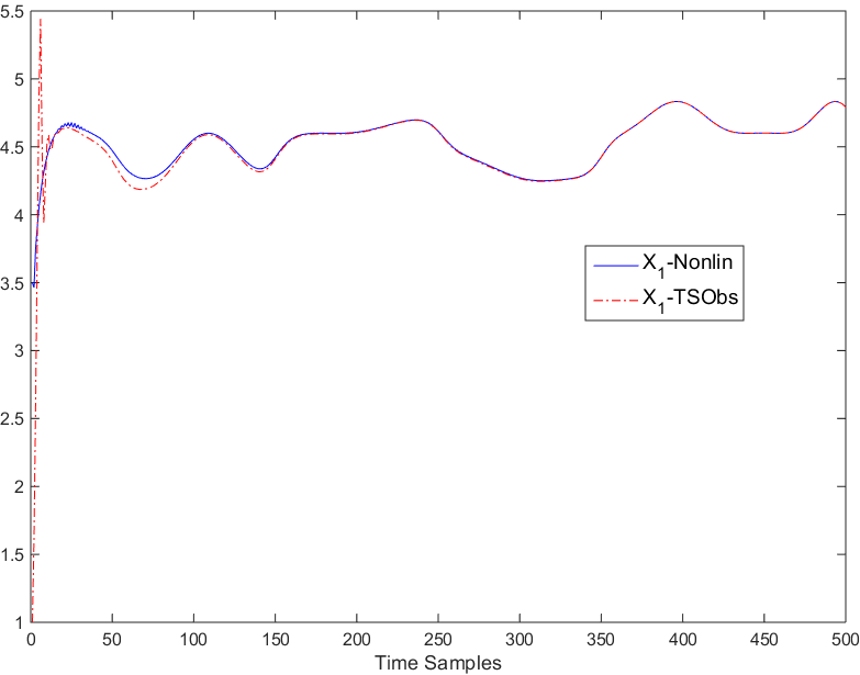
Figure 1: Estimation of x1,ksubscript𝑥1𝑘x_{1,k}

The unknown parameter θ𝜃\theta in (66) is constant; however, for the observer design purposes we assume it to be known and in the range,

θ[0.3,0.3]𝜃0.30.3\displaystyle\theta\in[-0.3,0.3] (74)

We choose the premise variables,

z1,k=uk,and,z2,k=x1,kx2,k+bformulae-sequencesubscript𝑧1𝑘subscript𝑢𝑘andsubscript𝑧2𝑘subscript𝑥1𝑘subscript𝑥2𝑘𝑏\displaystyle z_{1,k}=u_{k},\qquad\text{and},\qquad z_{2,k}=\frac{x_{1,k}}{x_{2,k}+b} (75)

It is evident that z2,ksubscript𝑧2𝑘z_{2,k} depends on the unmeasured state x2,ksubscript𝑥2𝑘x_{2,k} making it unmeasured. Assuming a range of values for uk[0,0.4]subscript𝑢𝑘00.4u_{k}\in[0,0.4], x1,k[0.01,6]subscript𝑥1𝑘0.016x_{1,k}\in[0.01,6], and x2,k[0.01,3]subscript𝑥2𝑘0.013x_{2,k}\in[0.01,3], we get the range of the premise variables as,

z1,k[0,0.4],z2,k[0.003,14.63]formulae-sequencesubscript𝑧1𝑘00.4subscript𝑧2𝑘0.00314.63\displaystyle z_{1,k}\in[0,0.4],\qquad z_{2,k}\in[0.003,14.63] (76)
Refer to caption
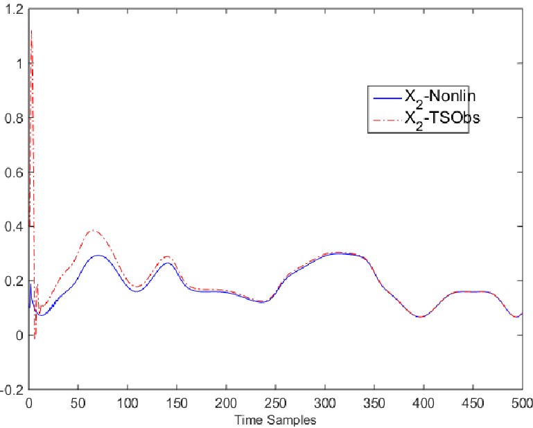
Figure 2: Estimation of x2,ksubscript𝑥2𝑘x_{2,k}

With these parameters, we get the model

𝐱k+1subscript𝐱𝑘1\displaystyle\mathbf{x}_{k+1} =i=18hi(𝐳k,θk)[Ai𝐱k+Biuk]absentsuperscriptsubscript𝑖18subscript𝑖subscript𝐳𝑘subscript𝜃𝑘delimited-[]subscript𝐴𝑖subscript𝐱𝑘subscript𝐵𝑖subscript𝑢𝑘\displaystyle=\sum_{i=1}^{8}h_{i}(\mathbf{z}_{k},\theta_{k})\left[A_{i}\mathbf{x}_{k}+B_{i}u_{k}\right] (77)

where hi(𝐳k,θ)subscript𝑖subscript𝐳𝑘𝜃h_{i}(\mathbf{z}_{k},\theta) is obtained from the product of membership functions of z1,ksubscript𝑧1𝑘z_{1,k}, z2,ksubscript𝑧2𝑘z_{2,k} and θ𝜃\theta corresponding to the submodel i𝑖i. The system matrices are given by,

A1subscript𝐴1\displaystyle A_{1} =[15.9×10400.99]A2=[10.002400.99]A3=[12.9200.17]absentmatrix15.9superscript10400.99subscript𝐴2matrix10.002400.99subscript𝐴3matrix12.9200.17\displaystyle=\begin{bmatrix}1&5.9\times 10^{-4}\\ 0&0.99\end{bmatrix}A_{2}=\begin{bmatrix}1&0.0024\\ 0&0.99\end{bmatrix}A_{3}=\begin{bmatrix}1&2.92\\ 0&-0.17\end{bmatrix}
A4subscript𝐴4\displaystyle A_{4} =[111.703.68]A5=[0.65.9×10400.6]A6=[0.60.002400.6]absentmatrix111.703.68subscript𝐴5matrix0.65.9superscript10400.6subscript𝐴6matrix0.60.002400.6\displaystyle=\begin{bmatrix}1&11.7\\ 0&-3.68\end{bmatrix}A_{5}=\begin{bmatrix}0.6&5.9\times 10^{-4}\\ 0&0.6\end{bmatrix}A_{6}=\begin{bmatrix}0.6&0.0024\\ 0&0.6\end{bmatrix}
A7subscript𝐴7\displaystyle A_{7} =[0.62.9300.57]A8=[0.611.704.1]and,Bi=[02],iformulae-sequenceabsentmatrix0.62.9300.57subscript𝐴8matrix0.611.704.1andsubscript𝐵𝑖matrix02for-all𝑖\displaystyle=\begin{bmatrix}0.6&2.93\\ 0&-0.57\end{bmatrix}A_{8}=\begin{bmatrix}0.6&11.7\\ 0&-4.1\end{bmatrix}\ \text{and},\qquad B_{i}=\begin{bmatrix}0\\ 2\end{bmatrix},\ \forall i
Refer to caption
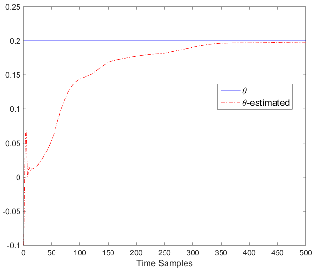
Figure 3: Estimation of θksubscript𝜃𝑘\theta_{k}

We used Matlab with Yalmip [lofberg2004yalmip] interface with LMIlab toolbox to solve the LMI conditions.

Remark 6.1.

Some problem specific conditions could be added to obtain an optimum solution to the problem. For example, pole placement for the state observers AiLiCsubscript𝐴𝑖subscript𝐿𝑖𝐶A_{i}-L_{i}C could be added as a separate LMI condition so as to achieve favourable rate of convergence. Further, some minimum value for the gain corresponding to parameter estimation, Ki,isubscript𝐾𝑖for-all𝑖K_{i},\forall i could be imposed so that the innovation term is useful in augmenting the estimated θ𝜃\theta (due to the relative scaling between the values of θ^^𝜃\hat{\theta} and yy^𝑦^𝑦y-\hat{y}). Further, as noted in Remark 4.7, the value of Qesubscript𝑄𝑒Q_{e} was chosen as

Qe=[0.001Inx000.1Inθ]subscript𝑄𝑒matrix0.001subscript𝐼subscript𝑛𝑥000.1subscript𝐼subscript𝑛𝜃\displaystyle Q_{e}=\begin{bmatrix}0.001I_{n_{x}}&0\\ 0&0.1I_{n_{\theta}}\end{bmatrix}
Remark 6.2.

It is to be noted that there are a number of variables to be determined by the LMI solver. This could be reduced by fixing some of the parameters. For this example, we chose the values for Γ2x=Γ2u=0.1superscriptsubscriptΓ2𝑥superscriptsubscriptΓ2𝑢0.1\Gamma_{2}^{x}=\Gamma_{2}^{u}=0.1 and λi=0.001,i=1,2,3,4formulae-sequencesubscript𝜆𝑖0.001for-all𝑖1234\lambda_{i}=0.001,\ \forall i=1,2,3,4. The significantly reduces the computational complexity of the problem.

With the above conditions, we obtain the following observer gain values,

L1subscript𝐿1\displaystyle L_{1} =[0.230.24]L2=[0.230.24]L3=[0.310.21]L4=[0.610.09]absentmatrix0.230.24subscript𝐿2matrix0.230.24subscript𝐿3matrix0.310.21subscript𝐿4matrix0.610.09\displaystyle=\begin{bmatrix}0.23\\ 0.24\end{bmatrix}L_{2}=\begin{bmatrix}0.23\\ 0.24\end{bmatrix}L_{3}=\begin{bmatrix}0.31\\ 0.21\end{bmatrix}L_{4}=\begin{bmatrix}0.61\\ 0.09\end{bmatrix}
L5subscript𝐿5\displaystyle L_{5} =[0.410.30]L6=[0.410.30]L7=[0.410.30]L8=[0.270.24]absentmatrix0.410.30subscript𝐿6matrix0.410.30subscript𝐿7matrix0.410.30subscript𝐿8matrix0.270.24\displaystyle=\begin{bmatrix}-0.41\\ 0.30\end{bmatrix}L_{6}=\begin{bmatrix}-0.41\\ 0.30\end{bmatrix}L_{7}=\begin{bmatrix}-0.41\\ 0.30\end{bmatrix}L_{8}=\begin{bmatrix}-0.27\\ 0.24\end{bmatrix}

and Ki=0.03,isubscript𝐾𝑖0.03for-all𝑖K_{i}=0.03,\ \forall i.

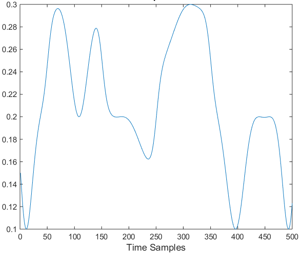
With these gain values, we obtain the state estimation results as shown in the Fig 1 and 2. The estimation of the unknown parameter is given in Fig 3. Further, the input used for the simulation is shown in the Fig 4.
Refer to caption
Figure 4: Input used for simulation

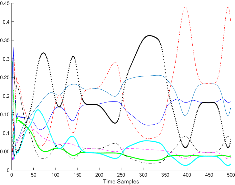
To illustrate the nonlinearity of the model, we show the variation of the weighting function hi(x^,θ^)subscript𝑖^𝑥^𝜃h_{i}(\hat{x},\hat{\theta}) in the Fig 5.

7 Concluding Remarks

We presented an adaptive observer design procedure for discrete-time nonlinear systems which could be converted to a quasi-LPV form. The presented work fills a gap for adaptive observer design for discrete-time nonlinear systems for those cases where the transformed quasi-LPV matrices depend on one of the unmeasured states of the system. The results in this approach are conservative, but provides an opening in exploring a systematic approach for adaptive observer design for nonlinear system of this type. One interesting extension could be to explore other observer structures, especially the one proposed in [guyader2003adaptive] and follow the similar design strategy of our work so as to expand for unmeasured premise variable case.
Refer to caption
Figure 5: Weighting functions of the submodels

References

  • [1] \harvarditemBesançon2000besancon_remarks_2000 Besançon, G. \harvardyearleft2000\harvardyearright. Remarks on nonlinear adaptive observer design, Systems & Control Letters 41(4): 271–280.
  • [2] \harvarditem[Bezzaoucha et al.]Bezzaoucha, Marx, Maquin \harvardand Ragot2013abezzaoucha2013state Bezzaoucha, S., Marx, B., Maquin, D. \harvardand Ragot, J. \harvardyearleft2013a\harvardyearright. State and parameter estimation for nonlinear systems: a Takagi-Sugeno approach, American Control Conference, ACC’2013.
  • [3] \harvarditem[Bezzaoucha et al.]Bezzaoucha, Marx, Maquin \harvardand Ragot2013bbezzaoucha2013state2 Bezzaoucha, S., Marx, B., Maquin, D. \harvardand Ragot, J. \harvardyearleft2013b\harvardyearright. State and parameter estimation for time-varying systems: a Takagi-Sugeno approach, 5th Symposium on System Structure and Control, IFAC Joint Conference 2013 SSSC, TDS, FDA.
  • [4] \harvarditemBlanco2001blanco2001stabilisation Blanco, Y. \harvardyearleft2001\harvardyearright. Stabilisation des Modeles Takagi-Sugeno et leur usage pour la commande des systemes non lineaires, PhD thesis, Université des Sciences et Technologies de Lille. (in French).
  • [5] \harvarditem[Boyd et al.]Boyd, El Ghaoui, Feron \harvardand Balakrishnan1994boyd1994linear Boyd, S. P., El Ghaoui, L., Feron, E. \harvardand Balakrishnan, V. \harvardyearleft1994\harvardyearright. Linear matrix inequalities in system and control theory, Vol. 15, SIAM.
  • [6] \harvarditem[Caccavale et al.]Caccavale, Pierri \harvardand Villani2008caccavale2008adaptive Caccavale, F., Pierri, F. \harvardand Villani, L. \harvardyearleft2008\harvardyearright. Adaptive observer for fault diagnosis in nonlinear discrete-time systems, Journal of dynamic systems, measurement, and control 130(2): 021005.
  • [7] \harvarditemCho \harvardand Rajamani1997cho_systematic_1997 Cho, Y. M. \harvardand Rajamani, R. \harvardyearleft1997\harvardyearright. A systematic approach to adaptive observer synthesis for nonlinear systems, IEEE Transactions on Automatic Control 42(4): 534–537.
  • [8] \harvarditemŢiclea \harvardand Besançon2013ticlea_exponential_2013 Ţiclea, A. \harvardand Besançon, G. \harvardyearleft2013\harvardyearright. Exponential forgetting factor observer in discrete time, Systems & Control Letters 62(9): 756–763.
  • [9] \harvarditemŢiclea \harvardand Besançon2016ticlea_adaptive_2016 Ţiclea, A. \harvardand Besançon, G. \harvardyearleft2016\harvardyearright. Adaptive observer design for discrete time LTV systems, International Journal of Control 89(12): 2385–2395.
  • [10] \harvarditemde Souza \harvardand Xie1992de1992discrete de Souza, C. E. \harvardand Xie, L. \harvardyearleft1992\harvardyearright. On the discrete-time bounded real lemma with application in the characterization of static state feedback Hsubscript𝐻{H}_{\infty} controllers, Systems & Control Letters 18(1): 61–71.
  • [11] \harvarditemGuyader \harvardand Zhang2003guyader2003adaptive Guyader, A. \harvardand Zhang, Q. \harvardyearleft2003\harvardyearright. Adaptive observer for discrete time linear time varying systems, 13th IFAC/IFORS Symposium on System Identification, SYSID’2003.
  • [12] \harvarditem[Ichalal et al.]Ichalal, Marx, Maquin \harvardand Ragot2016ichalal2016method Ichalal, D., Marx, B., Maquin, D. \harvardand Ragot, J. \harvardyearleft2016\harvardyearright. A method to avoid the unmeasurable premise variables in observer design for discrete time ts systems, International Conference on Fuzzy Systems, FUZZ-IEEE’2016.
  • [13] \harvarditem[Ichalal et al.]Ichalal, Marx, Ragot \harvardand Maquin2009ichalal2009state Ichalal, D., Marx, B., Ragot, J. \harvardand Maquin, D. \harvardyearleft2009\harvardyearright. State and unknown input estimation for nonlinear systems described by Takagi-Sugeno models with unmeasurable premise variables, 17th Mediterranean Conference on Control and Automation, MED’09.
  • [14] \harvarditem[Kwiatkowski et al.]Kwiatkowski, Boll \harvardand Werner2006kwiatkowski_automated_2006 Kwiatkowski, A., Boll, M. T. \harvardand Werner, H. \harvardyearleft2006\harvardyearright. Automated Generation and Assessment of Affine LPV Models, Proceedings of the 45th IEEE Conference on Decision and Control.
  • [15] \harvarditem[Lendek et al.]Lendek, Guerra \harvardand De Schutter2010lendek2010stability Lendek, Z., Guerra, T. M. \harvardand De Schutter, B. \harvardyearleft2010\harvardyearright. Stability analysis and nonlinear observer design using Takagi-Sugeno fuzzy models, Vol. 262, Springer.
  • [16] \harvarditemLöfberg2004lofberg2004yalmip Löfberg, J. \harvardyearleft2004\harvardyearright. Yalmip: A toolbox for modeling and optimization in matlab, International Symposium on Computer Aided Control Systems design.
  • [17] \harvarditem[Nagy et al.]Nagy, Mourot, Marx, Ragot \harvardand Schutz2010nagy2010systematic Nagy, A. M., Mourot, G., Marx, B., Ragot, J. \harvardand Schutz, G. \harvardyearleft2010\harvardyearright. Systematic multimodeling methodology applied to an activated sludge reactor model, Industrial & Engineering Chemistry Research 49(6).
  • [18] \harvarditem[Ohtake et al.]Ohtake, Tanaka \harvardand Wang2003ohtake2003fuzzy Ohtake, H., Tanaka, K. \harvardand Wang, H. O. \harvardyearleft2003\harvardyearright. Fuzzy modeling via sector nonlinearity concept, Integrated Computer-Aided Engineering 10(4): 333–341.
  • [19] \harvarditem[Srinivasarengan et al.]Srinivasarengan, Ragot, Maquin \harvardand Aubrun2016asrinivasarengan:hal-01399791 Srinivasarengan, K., Ragot, J., Maquin, D. \harvardand Aubrun, C. \harvardyearleft2016a\harvardyearright. Joint state and parameter estimation for discrete-time Takagi-Sugeno model, 13th European Workshop on Advanced Control and Diagnosis, ACD 2016.
  • [20] \harvarditem[Srinivasarengan et al.]Srinivasarengan, Ragot, Maquin \harvardand Aubrun2016bsrinivasarengan2016nonlinear Srinivasarengan, K., Ragot, J., Maquin, D. \harvardand Aubrun, C. \harvardyearleft2016b\harvardyearright. Nonlinear joint state-parameter observer for VAV damper position estimation, 3rd Conference on Control and Fault-Tolerant Systems, SysTol 2016.
  • [21] \harvarditemTanaka \harvardand Wang2004tanaka2004fuzzy Tanaka, K. \harvardand Wang, H. O. \harvardyearleft2004\harvardyearright. Fuzzy control systems design and analysis: a linear matrix inequality approach, John Wiley & Sons.
  • [22] \harvarditemThumati \harvardand Sarangapani2008thumati_model_2008 Thumati, B. T. \harvardand Sarangapani, J. \harvardyearleft2008\harvardyearright. A model based fault detection scheme for nonlinear multivariable discrete-time systems, 2008 IEEE International Conference on Systems, Man and Cybernetics, pp. 1978–1983.
  • [23] \harvarditemZhang2002zhang2002adaptive Zhang, Q. \harvardyearleft2002\harvardyearright. Adaptive observer for multipleinputmultipleoutput (mimo) linear time-varying systems, IEEE Transactions on Automatic Control 47(3): 525–529.
  • [24] \harvarditemZhou \harvardand Khargonekar1988zhou1988robust Zhou, K. \harvardand Khargonekar, P. P. \harvardyearleft1988\harvardyearright. Robust stabilization of linear systems with norm-bounded time-varying uncertainty, Systems & Control Letters 10(1): 17–20.
  • [25]