Hubble Frontier Fields: systematic errors in strong lensing models of galaxy clusters - Implications for cosmography
Abstract
Strong gravitational lensing by galaxy clusters is a fundamental tool to study dark matter and constrain the geometry of the Universe. Recently, the HST Frontier Fields program has allowed a significant improvement of mass and magnification measurements but lensing models still have a residual RMS between 0.2" and few arcseconds, not yet completely understood. Systematic errors have to be better understood and treated in order to use strong lensing clusters as reliable cosmological probes. We have analysed two simulated Hubble Frontier Fields-like clusters from the Hubble Frontier Fields Comparison Challenge, Ares and Hera. We use several estimators (relative bias on magnification, density profiles, ellipticity and orientation) to quantify the goodness of our reconstructions by comparing our multiple models, optimized with the parametric software Lenstool, with the input models. We have quantified the impact of systematic errors arising, first, from the choice of different density profiles and configurations and, secondly, from the availability of constraints (spectroscopic or photometric redshifts, redshift ranges of the background sources) in the parametric modelling of strong lensing galaxy clusters and therefore on the retrieval of cosmological parameters. We find that substructures in the outskirts have a significant impact on the position of the multiple images, yielding tighter cosmological contours. The need for wide-field imaging around massive clusters is thus reinforced. We show that competitive cosmological constraints can be obtained also with complex multimodal clusters and that photometric redshifts improve the constraints on cosmological parameters when considering a narrow range of (spectroscopic) redshifts for the sources.
keywords:
Gravitational Lensing: strong – Cosmology: Cosmological Parameters – Galaxies: clusters: general1 Introduction
Strong gravitational Lensing (SL, hereafter) is nowadays at the very heart of important issues in modern cosmology, allowing for instance to measure directly the total projected mass distribution (baryonic and dark) of galaxy cluster cores (e.g. Richard et al., 2010; Zitrin &
Broadhurst, 2016; Monna
et al., 2017; Mahler
et al., 2017), to image very high redshift sources otherwise too faint to be detected without the gravitational magnification (Kneib et al., 2004; Richard et al., 2008; Coe et al., 2013; Atek
et al., 2015) and to constrain the geometry of the Universe (Jullo et al., 2010; D’Aloisio &
Natarajan, 2011; Magaña et al., 2015; Caminha
et al., 2016) which is one of the long-standing challenges of modern cosmology.
In the standard cosmological model , 72 of the energy density of the Universe is in the form of a ’dark energy’, a fluid with negative pressure that would cause the presently acceleration of the Universe (Planck
Collaboration et al., 2016a).
Type Ia supernovae (Riess
et al., 1998), baryon acoustic oscillations (Beutler
et al., 2011; Gil-Marín
et al., 2016), cosmic shear (Massey
et al., 2007; Heymans
et al., 2012; Hildebrandt
et al., 2017), cluster abundances (de Haan
et al., 2016), CMB anisotropies (Planck
Collaboration et al., 2016a) or time delays (Suyu
et al., 2016) are some of the several probes allowing to better understand the constituents of the Universe and their properties by putting tighter constraints on cosmological parameters.
However, in order to obtain robust estimates of cosmological parameters, estimates from the different cosmological probes must be combined as each technique has distinct degeneracies and biases (Planck
Collaboration et al., 2016b; Peel et al., 2017).
Among the previously mentioned cosmological probes, using the strong lensing features in galaxy clusters is a very promising technique that yields orthogonal constraints in an era of precise cosmology (Golse
et al., 2002; Gilmore &
Natarajan, 2009; Jullo et al., 2010). To perform cosmography with strong lenses, a precise and accurate mass distribution of the cluster is required, i.e, a large number of constraints is crucial.
Recently, the Hubble Frontier Fields program111http://www.stsci.edu/hst/campaigns/frontier-fields (HFF; P.I.: J. Lotz, Lotz
et al., 2017) with the Hubble Space Telescope (hereafter HST) has provided the deepest multi-colour imaging of galaxy clusters to date, that combined with spectroscopy from ground-based surveys, has led to the discovery of hundreds of multiple images and thus to a significant improvement of cluster mass estimates (Jauzac
et al., 2014; Diego et al., 2016; Lagattuta
et al., 2016; Monna
et al., 2017).
The mass modelling of strong lensing clusters can be carried out in different manners: parametric and non-parametric methods are equally used; the primary distinction between them being that parametric modelling assumes that luminous cluster galaxies trace the cluster mass whereas non-parametric does not.
The FF-SIMS Challenge (Meneghetti
et al., 2016), an archive of mock HFF-like clusters, has provided the lensing community with a set of simulated clusters in order to highlight for the first time the strengths and weaknesses of each methods: parametric and non-parametric. This work would allow the non-lensing community to choose a method and software according to their different needs. This challenge has shown that all lensing reconstruction methods provide reliable mass distributions.
However, strong lensing modelling appears to be still unable to match the HST observations angular resolution ( 0.05") with a residual RMS between 0.2" and a few arcseconds (Limousin
et al., 2016), a systematical error not yet completely understood and few studies have addressed this issue.
Indeed, strong lensing mass modelling has various sources of systematic errors, arising from the hypothesis behind our models, which have recently started to be acknowledged and analysed in a more quantitative way. Meneghetti et al. (2010) studied the properties of strong lensing clusters in the MARENOSTRUM cosmological simulation. They find that strong lenses tend to have their major axes oriented along the line of sight. This orientation bias results for instance in cluster concentrations estimations from the projected density profiles to be biased high (Giocoli et al., 2014; Sereno et al., 2015). D’Aloisio &
Natarajan (2011) quantified that the modelling errors due to the scatter in the cluster-galaxy scaling relations and unmodelled line-of-sight haloes can result in errors of the order of a few arcseconds on average. Bayliss
et al. (2015) studied the impact of assuming a certain cosmological model on the determination of magnification and mass profiles of the cluster core for HFF clusters showing that cosmological parameter uncertainty is a non-negligible source of errors for the lens modelling.
Foreground or background large-scale structures impacts the SL modelling as well (Dalal
et al., 2005; Host, 2012), that could introduce a systematic error of up to on the position of multiple images (Zitrin
et al., 2015). Line of sight effects have then to be taken into account during the strong lensing modelling in order to recover precise cosmological parameters (Jullo et al., 2010; Caminha
et al., 2016).
Systematic errors can also arise from the mass distributions assumed for the dark matter components as shown in Limousin
et al. (2016) where the observed constraints in MACS0717 are equally well reproduced by a mass model with a shallow large-scale DM component and one for which this component is peaky. Harvey
et al. (2016) analysed the FF cluster MACSJ0416 () and found that the assumption that light traces mass can introduce an error of 0.5" on the position of the multiple images. Bouwens et al. (2016) studied the impact of magnification uncertainties on luminosity functions from the first four HFF clusters. Johnson &
Sharon (2016) have led the first investigation attempting to quantify systematic errors induced by the availability of constraints in strong lensing clusters. They show that the accuracy of the magnification is sensitive to the selection of constraints rather than their amount.
In this paper we take advantage of the mock HFF-like clusters archive from the FF-SIMS Challenge and use two of the HFF-like mock strong lensing clusters (Ares and Hera) to investigate how systematic errors in the strong lensing parametric modelling with Lenstool affect the determination of the total mass distribution in clusters and hence the retrieval of robust cosmological parameters such as the mean matter density and dark energy equation of state parameters and , respectively.
First, we use four different estimators (density profiles, relative bias on magnification, cluster’s ellipticity and orientation angle) to compare our reconstructions with the input models in order to assess the impact of different mass distributions and configurations in the strong lensing modelling of clusters and hence on the cosmography.
Secondly, we study how the availability of constraints affects the retrieval of unbiased cosmological parameters. We investigate if there is a more efficient range of redshifts to recover the input cosmology, if including photometric redshifts can result in a more robust estimation of these parameters and if taking into account an increasing number of photometric families translates into an increasing precision in the cosmological parameters estimation.
The paper is organized as follows: the data used for this analysis is presented in Section 2, in Section 3 we describe the methodology, in Section 4 we detail the different modellings for Ares and Hera, we then show the systematic uncertainties in Section 5, their impact on cosmography in Section 6 and conclude in Section 7.
Throughout the paper, we use the standard flat cosmological model with the Hubble constant , and are let as free parameters. Magnitudes are quoted in the AB system.
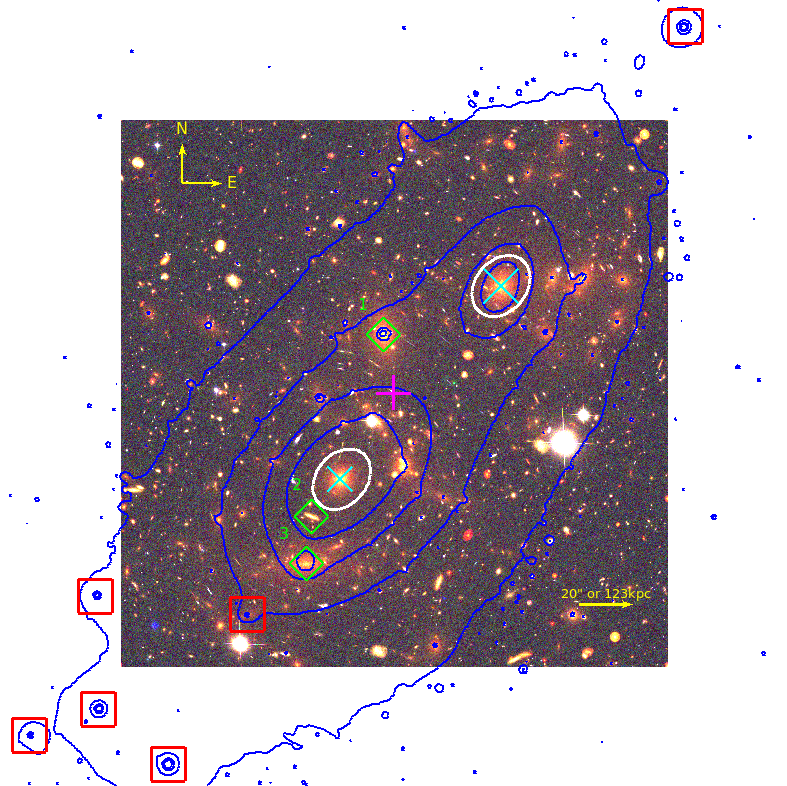
Upper panel: Ares cluster. The cluster’s centre is indicated by the magenta cross. Large-scale potentials are shown as white ellipses, BCGs as cyan crosses, galaxy haloes as green diamonds and red boxes for the outskirts substructures.
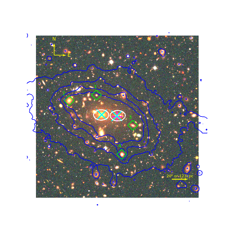
Bottom panel: Hera cluster. Same colour code as for Ares.
2 The Data
We have analysed two mock HFF-like clusters from the FF-simulations Challenge archive (Meneghetti
et al., 2016):
Ares and Hera. They were initially created for the lens modelling comparison project, which, for the first time, compares the reconstructions obtained using different techniques, such as parametric, non-parametric and hybrid, performed by different teams.
Both clusters have been simulated to reproduce, not only the characteristics of the HST Advandced Camera for Survey (ACS) and Wide-Field Camera 3 (WFC3) observations (depth, passbands and spatial resolution), but also the complexity of the FF clusters themselves even if these two have been created using different techniques.
Both clusters have then been modelled to be realistic, complex, bi-modal clusters (see Figure 1), generated in a flat cosmological model.
During the challenge, all participants first performed a blind analysis (i.e, not knowing the true mass distribution) of these clusters for which only the HFF-like images as well as catalogues of multiple images (position and spectroscopic redshifts) and cluster galaxies (positions and magnitudes in all ACS/WFC3 bands) were provided with (see Table 1 for further details).
Ares is a more powerful lens than Hera, producing thus many more multiple images (Meneghetti
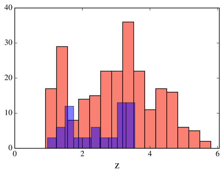
et al., 2016). Their respective redshift distributions are shown in Figure 11. The source galaxies resemble the luminosity and the redshift distribution of the galaxies in the Hubble Ultra-Deep-Field (Coe et al., 2006).
For both clusters, the software Skylens (Meneghetti
et al., 2008) was used to ray-trace the lensed galaxies to the image plane and to create simulated HFF-like images in all bands.
After the unblinding, the convergence and shear maps (calculated for a source at =9) were provided. They were used to compare our reconstructions with the true values and also to improve our models. The input cosmology was also revealed.
We refer the reader to Meneghetti
et al. (2016) for a detailed presentation on how Ares and Hera mass distributions were generated, here we only present a quick overview.
2.1 Ares
Ares is a semi-analytical cluster (created using MOKA222https://cgiocoli.wordpress.com/research-interests/moka/ by Giocoli et al., 2012) at z=0.5. This simulated cluster is built with three components: two smooth dark matter triaxial haloes with a NFW profile, a bright central cluster galaxy (BCG) with an Hernquist profile (Hernquist, 1990) and sub-haloes having a Singular Isothermal Sphere profile (Hernquist, 1990). Dark matter sub-haloes are populated using a Halo Occupation Distribution technique (HOD) and stellar and B-band luminosities are given for all galaxies according to the mass of their sub-halo as in Wang et al. (2006).
The mass within the virial radius is then defined as .
Ares is generated in a flat cosmological model with a matter density parameter .
2.2 Hera
Hera is from a N-body simulation of cluster-sized dark matter halos for a flat model (see Planelles
et al., 2014) at z=0.507 which was re-simulated using a TreePM-SPH GADGET-3 code with only collision-less dark matter particles. The properties of cluster galaxies are created from Semi-Analytic Methods of galaxy formation (De Lucia &
Blaizot, 2007).
Hera is also created in a flat cosmological model with a matter density parameter .
| Cluster name | Cluster galaxies | Images | Sources | |
|---|---|---|---|---|
| Ares | 0.5 | 330 | 242 | 85 |
| Hera | 0.507 | 337 | 65 | 19 |
For both clusters, the software Skylens (Meneghetti
et al., 2008) was used to ray-trace the lensed galaxies to the image plane and to create simulated HFF-like images in all bands.
3 Methodology
3.1 Mass modelling
We perform the strong lensing modelling in the source plane using the public software Lenstool333https://projets.lam.fr/projects/lenstool (Kneib et al., 1996; Jullo
et al., 2007) which performed very well for the FF-SIMS Challlenge. Lenstool utilizes a Bayesian Markov chain Monte-Carlo (hereafter MCMC, see Jullo
et al., 2007, for details) sampler to optimize the model using the positions of the multiply imaged systems. The matter distribution of clusters is decomposed into several smooth large scale components and individual contributions from cluster galaxies. In this work, the reconstructions are based on the strong lensing information only.
We have modelled both clusters as up to three components: i) large-scale potentials, ii) brightest cluster galaxies (BCGs) and iii) individual galaxies identified spectroscopically, with masses scaling with luminosity. Each mass component has a parameterized profile such as the Pseudo Isothermal Elliptical Mass Distribution (Kassiola &
Kovner, 1993, hereafter PIEMD), Navarro, Frenk & White (NFW) (Navarro
et al., 1997) or Hernsquist (Hernquist, 1990). For instance, large-scale potentials are modelled with either a NFW or PIEMD, BCGs with PIEMD or Hernquist profiles and individual clusters members with a PIEMD profile, scaled according to the relations in Limousin et al. (2005). These mass distributions are briefly presented hereafter.
We used the NFW density profile (Navarro et al., 1997) to model Ares and Hera large-scale mass distributions. The 3D density profile is given by:
| (1) |
where is a characteristic density and is the scale radius.
This profile behaves as in the inner region, at and as in the outer regions.
In Lenstool, this profile has the following free parameters: x and y, the
coordinates of the halo centre; e, the ellipticity, defined as e = with a and b the semi-major and semi-minor axis respectively and , the position angle (counted counter-clockwise from the x axis); , the scale radius and , the velocity dispersion.
The pseudo isothermal density profile (Limousin et al., 2005) is used to model dark matter haloes and/or individual galaxies which 3D density distribution is given by:
| (2) |
with a core radius and a truncation radius .
This profile is characterized by two changes in the density slope: within the transition region ( < r < ) it behaves as an isothermal profile with , while exiting this region, the density will fall as (such behaviour is common for elliptical galaxies).
It has the following free parameters: the coordinates x, y; the ellipticity, e; angle position, ; core and cut radii, and and a velocity dispersion, .
We use the Hernquist profile (Hernquist, 1990) to model the BCGs of the two clusters. BCGs are massive elliptical galaxies with observed luminosities well represented by the de Vaucouleurs empirical law (which fits well observations) but being more simple analytically. The 3D density profile of te Hernquist profile can be written as follows:
| (3) |
where is the total mass and , the characteristic scale length. This profile is extremely similar to the NFW profile at small radii but the density falls as at larger radii.
It is parametrized using the following free parameters: the coordinates x, y; the ellipticity, e; angle position, ; a core radius, and a velocity dispersion, .
Once the mass components are defined, the best-fitting model parameters are found by minimizing the distance between the observed and model-predicted positions of the multiple images, and the parameter covariance is estimated using a Bayesian Markov Chain Monte Carlo (MCMC) technique (Jullo et al., 2007). For each of the models, we use several statistical values to assess the goodness of the fit and to discriminate between models.
-
1.
We use the root-mean-square between the observed and predicted positions of the multiple images from the modelling, computed as follows:
(4) where and are the observed and model-predicted positions of the multiples images and N being the total number of images.
-
2.
We compute the Bayesian Information Criterion (BIC, introduced by Schwarz, 1978):
(5) with , the likelihood; , the number of free parameters and , the number of constraints.
-
3.
The corrected Akaike Information Criterion (AICc). The BIC will over-penalize models whereas AICc tends to under-penalize. Using the two together helps balancing those effects. It is computed as follows:
(6) -
4.
The reduced , see Jullo et al. (2007) for details.
-
5.
The Bayesian Evidence which considers the ’complexity’ of the models and how this ’complexity’ is justified by the observables, see also Jullo et al. (2007) for details.
3.2 Cosmological parameters
As both Ares and Hera have a large number of multiple images with spectroscopic redshifts for all images -up to redshift for Ares and for Hera (see Figure 11)- they represent good probes to constrain cosmological parameters.
We briefly outline here the methodology to estimate these parameters with cluster strong lensing (further details can be found in Golse
et al., 2002; Gilmore &
Natarajan, 2009, for instance).
Strong lensing is sensitive to the underlying geometry of the Universe as the position of the multiple images not only depends on the mass distribution of the lens, but also on the angular diameter distances from the observer to the lens (), to the source (), and from the lens to the source (). This dependence is used to put constraints on the cosmological parameters and .
Indeed, the lens equation can be written as:
| (7) |
where and are the (multiple) image angular positions in the lens and source planes respectively, is the projected Newtonian potential of the lens and the cosmological dependence is embedded into the angular diameter distances.
When only one family of multiple images is available, the ratio between the cosmological distances cannot be disentangled from the gradient of the potential. However, if at least 2 systems of images at different redshifts are available, this degeneracy can be broken and via the ’family ratio’ (see Link &
Pierce, 1998) from which constraints on and can be obtained:
| (8) |
with is the redshift of the lens, and are the redshifts of two distinct source and is the angular diameter distance.
This kind of analysis has already been carried out for galaxy clusters Abell 2218, Abell 1689 and Abell S1063 (or RXC J2248.7-4431) by Soucail
et al. (2004); Jullo et al. (2010); Caminha
et al. (2016) respectively and also with simulated data (Golse
et al., 2002; Gilmore &
Natarajan, 2009; D’Aloisio &
Natarajan, 2011).
In this work, the energy density of the total matter of the universe and the equation-of-state parameter are set as free parameters in a flat cosmological model.
3.3 Priors
In this section we describe the choice of boundaries for the flat priors of the free parameters mentioned below. Some boundaries are set with a quite large interval. However others have more narrow priors.
The positions of the haloes (for both cluster- and galaxy- scale potentials), x and y, correspond to the light peak of galaxies (the position of the BCGs being the central coordinates for the dark matter haloes). The angle position of haloes are also set by the luminous component’s angle. The ellipticity is not allowed to reach very high values following Despali et al. (2017). This work shows that high ellipticities () are not favored by theoretical predictions.
Finally, some parameters have quite narrow priors as models have been run several times and in order to gain in computing time some prior ranges were tighten, checking that the boundaries were not reached.
Nonetheless, we checked that a slight change in the boundaries had no impact on the posterior distribution of the parameters.
4 Strong lensing models
We here present the details of each model for the Ares and Hera clusters, the free parameters for each potential and the respective flat priors.
These models are presented in chronological order as we tried to model the clusters in a more complex way (and also after the unblinding of the true mass profiles).
Their id number throughout the paper is the last number of their corresponding subsection. The first term stands for the density profile used for the large-scale haloes, the second (if any) for BCGs.
All coordinates are presented as the distance to the centre of the clusters (in arcseconds) shown as the magenta cross in Figure 1. The centre has been arbitrarily chosen to be ()= (0", 0") and serves as reference for Lenstool.
4.1 Ares
Thanks to the HST simulated images, we easily see that this cluster is bimodal, all the models thereafter will have two large-scale haloes whose coordinates stated below correspond to those of the light peaks (see upper panel of Figure 1).
Cluster member galaxies are taken from the given simulated catalogues up to a magnitude of < 22.0 (being a more complex cluster, we limited the sample with a magnitude cut to gain in computing time, representing of the total cluster luminosity) and the small scale haloes associated to galaxy members are parametrized with a PIEMD profile with a fixed core radius of 0.15 kpc, a velocity dispersion allowed to vary between 94 and 180 km/s, a cut radius varying from 78 kpc to 272.00 kpc, considered spherical, with a (the reference magnitude for the scaling relations corresponding to at the cluster’s redshift) and following the scaling relations (Faber &
Jackson, 1976).
Moreover, three massive galaxies were more carefully modelled (shown as green diamonds in Figure 1) also using a PIEMD density profile. These massive galactic haloes were modelled independently (not using the scaling relations) as they appeared to have a significant impact in the mass profile and/or on the nearby multiple images. For the three of them, the cut radius is fixed to 1000 kpc as initially the modelling was undertaken as the merger of four haloes (supported by the high velocity dispersions of these massives galaxies).
The first galaxy (labelled as 1 in Figure 1) is fixed at ()= (+4.053", +22.042") away from the centre of the cluster. Its ellipticity can go up to 0.6, the angle position is allowed to vary from 60.0 to 120.0 degrees and its velocity dispersion from 100.0 to 400.0 km/s.
The galaxy labelled as 2 in Figure 1 is located at ()= (+30.78", -45.98") away from the centre of the cluster with an ellipticity from 0.3 to 0.7, the angle position is allowed to vary from 0.0 to 90.0 degrees and its velocity dispersion from 50.0 to 400.0 km/s.
Finally, the galaxy labelled as 3 in Figure 1 is located at ()= (+33.008", -63.542") away from the centre of the cluster. From the input convergence contours it appeared as a massive halo. It is modelled with ellipticity with values between 0.1 - 0.7, the angle position is allowed to vary from 141 to 171 degrees and its velocity dispersion from 400.0 to 700.0 km/s.
All multiple images are included in the models with a positional uncertainty of 0.5" and the optimization is performed in the source plane as it is less computing time expensive. We checked that the results are similar with both source and image plane optimizations.
4.1.1 PIEMD
This first model contains two large-scale haloes whose coordinates are fixed at ()= (+20.0", -32.0") and (-40.0", +40.0") away from the centre of the cluster respectively. These clumps do not harbour any additional halo linked to the BCGs.
For the first clump, we let the core radius vary from 20 kpc to 65 kpc with a fixed cut radius of 1000 kpc. The ellipticity of this halo is allowed to reach values from 0.2 and as high as 0.7 and its orientation from 130 to 140 degrees and the velocity dispersion can vary from 400 to 1700 km/s.
The second large-scale halo can have a core radius with any value from 20 kpc to 60 kpc and the cut radius is fixed to 1000 kpc. Its ellipticity can take any value from 0.3 to 0.6, its orientation can vary from 105 to 115 degrees and the velocity dispersion can vary from 400 to 1000 km/s.
4.1.2 PIEMD - PIEMD
This reconstruction is the same as the previous one but we add two BCG components (modelled using the PIEMD profile) whose coordinates are fixed to main large-scale haloes’. These BCGs are modelled separately and do not follow the scaling relations (Newman
et al., 2013).
The BCG centred in the first clump ()= (+20.0", -32.0") can have a core radius between 3.5 and 50.0 kpc, the cut radius can vary from 25 to 320 kpc, the ellipticity from 0.2 to 0.7, the orientation from 120 to 180 degrees and the velocity dispersion from 100 to 500km/s.
As for the BCG centred at ()= (-40.0", +40.0"): its core radius can vary between 25 and 35 kpc, the cut radius from 670 to 730 kpc. Its ellipticity is allowed to vary between 0.4 and 0.65 kpc, the orientation angle from 105 to 115 degrees and the velocity dispersion from 80 to 420 km/s.
4.1.3 NFW
This reconstruction, as in 4.1.1, has two cluster-scale haloes but modelled using a NFW density profile instead.
The clump fixed at ()= (+20.0", -32.0") away from the cluster centre can have an orientation between 130 and 140 degrees, its velocity dispersion can vary between 500.0 and 2000.0 km/s and its scale radius varies from 50 to 280kpc and we let the ellipticity vary from 0.2 to 0.6.
The ellipticity of the second clump - fixed at ()= (-40.0", +40.0")- can reach values up to 0.6, the orientation is set between 105 and 115 degrees, the velocity dispersion is set to vary between 500 and 1800km/s and its scale radius between from 50 and 280kpc.
Even if the ellipticity intervals are quite large for both clumps, after optimization these clumps do no reach values . This is in agreement with Golse &
Kneib (2002) who demonstrated that the NFW profile is ill-defined for large ellipticities as defined in Lenstool. This will remain true for both clusters NFW models.
4.1.4 NFW - PIEMD
We add two BCG components (modelled with a PIEMD profile) to the reconstruction in 4.1.3, in the same way as in 4.1.2.
At this point, we realized that the NFW models were a better fit to ARES (than PIEMD for the large-scale haloes) as the improvement of the logarithm of the Evidence in Table 2 shows (confirmed as the profile used to generate Ares’s large-scale haloes upon the unblinding during the challenge). Therefore, the following models, more complex as they also take into account more distant structures or an Hernquist profile, were only modelled using the NFW profile for the large-scale haloes.
The last two models are "post-unblinding" models. Once the input convergence map was made available we discovered some structures in the outskirts of the cluster, out of the HST field of view (see Figure 1).
4.1.5 NFW - PIEMD + SUBS
This model, together with the model 4.1.7, includes six additional dark matter components located in the outskirts of the cluster.
This model is exactly like 4.1.4 with the additional substructures.
The substructures are located at ()= (+110.9", -118.4"); (+84.3", -138,8"); (+136.0", -127,98"); (+57.6", -83.2"); (-108,9", +136,9"); (+111.3", -75.0") away from the cluster’s centre. They are modelled with NFW profiles, considered as spherical, their velocity dispersions are allowed to vary between 100 and 500km/s and their scale radius between 20 and 200 kpc.
4.1.6 NFW - HERNQUIST
The large-scale clumps are modelled as in 4.1.4.
The BCGs, on the other hand have a different density profile: the Hernquist profile as described in Section 3.1.
The BCG located at ()= (+20.0", -32.0") has a core radius between 1.0 and 40.0 kpc. Its ellipticity can reach values up to 0.4, the orientation varies between 90 and 180 degrees and the velocity dispersion can vary from 100 to 400 km/s.
For the BCG located at ()= (-40.0", +40.0") the core radius is allowed to vary between 1.0 and 40.0 kpc, the ellipticity from 0.1 to 0.7, the orientation from 90 to 180 degrees and the velocity dispersion between 90 and 400 km/s.
4.1.7 NFW - HERNQUIST +SUBS
4.1.8 NFW - PIEMD + shapes
Last, we consider how taking into account the shapes of the galaxy-scale haloes impacts the reconstruction. The large-scale haloes and BCGs components are modelled as in 4.1.4 but we use SExtractor (Bertin & Arnouts, 1996) to measure the semi-major and semi-minor axis of the fitted ellipsis of each cluster galaxy which are then taken into account in the modelling.
4.2 Hera
In spite of the unimodal appearance of the cluster and its convergence contours in the bottom panel of Figure 1, Hera is also modelled as a bimodal cluster. Indeed, if this cluster is fitted with only one dark matter central clump the is twice larger.
The cluster members of the input catalogue were taken into account with < 24.0 and were modelled in the same way for all models: parametrized by a PIEMD profile with a fixed core radius of 0.15 kpc, a velocity dispersion allowed to vary between 60.0 and 100.0 km/s, a cut radius with values from 1.0 kpc to 200.00 kpc, considered spherical, with and following the scaling relations (Faber &
Jackson, 1976).
Moreover, in the same way as for Ares, four massive galaxies were more carefully modelled (indicated as green diamonds in Figure 1), using a PIEMD density profile and fitted in the same way for each model.
The galaxy labelled as 1 in Figure 1 is located at ()= (+25.91", +26.98") away from the cluster centre,considered spherical, an angle position of 72 degrees and a core radius of 0.07 kpc. Its cut radius can vary from 10.0 to 100.0 kpc and its velocity dispersion from 50.0 to 200.0 km/s.
The next one, labelled as 2 in Figure 1, is positioned at ()= (+60.38", +20.2"), with a core radius of 0.31 kpc. Its ellipticity can go up to 0.5, the angle position is set between -65.0 and 90.0 degrees, the cut radius can vary from 30.0 to 400.0 kpc and its velocity dispersion from 50.0 to 500.0 km/s.
The third halo of a massive galaxy (labelled as 3 in Figure 1) is located at ()= (-19.665", -11.078") with a core radius of 0.1 kpc. Its ellipticity can vary between 0.1 to 0.7, the angle position from 22 to 90 degrees, the cut radius is allowed to vary between 8.0 to 150 kpc and the velocity dispersion from 400 to 200.0 km/s.
Finally, the last one is a very massive galactic halo (labelled as 4 in Figure 1) having a significant impact in the total mass distribution profile. This halo is located at ()= (-7.0", -46.0") with a core radius of 0.1, an ellipticity set between 0.1 and 0.7, an angle position allowed to vary between 75.0 to 90.0 degrees, a cut radius between 8.0 and 250.0 kpc and a velocity dispersion between 40.0 and 600.0 km/s.
All the multiple images provided were included in the model with a positional uncertainty of 0.5" and the optimization is performed in the source plane. As for Ares we checked that image plane and source plane models were giving similar results.
4.2.1 PIEMD
This model contains two large-scale halos whose coordinates are placed at ()= (0.00", 0.00") and ()= (+20.0", +2.00") away from the centre of the cluster respectively (and no BCGs). They are allowed to move around by 2.00".
For the first clump, we let the core radius vary from 5 kpc to 37 kpc with a fixed cut radius of 3000 kpc. The ellipticity of this halo is allowed to vary values from 0.0 and 0.7, its orientation angle from 0.0 to 180.0 degrees and its velocity dispersion can vary from 400 to 1500 km/s.
The second dark matter clump can have a core radius with any value from 5 kpc to 40 kpc and cut radius, also fixed, of 3000 kpc. Its ellipticity can take any value from 0.0 to 0.7, its orientation can vary from 0.0 to 180 degrees and the velocity dispersion can vary from 600 to 1000 km/s.
4.2.2 PIEMD - PIEMD
We add two BCG components (modelled with a PIEMD profile) to the reconstruction in 4.2.1.
The BCG fixed at ()= (0.0", 0.0") has a fixed core radius of 0.5 kpc and a cut radius that can vary from 30.0 to 450.0 kpc. Its ellipticity can go from 0.0 to 0.4, the orientation from 5 to 90 degrees and the velocity dispersion from 100 to 500 km/s.
The ()= (+20.0", +2.00") centred BCG has a fixed core radius of 1.0 kpc, the cut radius can vary from 20.0 to 400.0 kpc, the ellipticity from 0.0 to 0.3, the orientation angle from 12.0 to 90.0 degrees and the velocity dispersion between 100 and 500 km/s.
4.2.3 PIEMD - HERNQUIST
In this reconstruction, the two added BCGs to the model 4.2.1 are modelled using an Hernquist density profile.
The BCG located at ()= (0.0", 0.0") has a fixed core radius of 0.5kpc. Its ellipticity can reach values up to 0.4, the orientation angle is allowed to vary from 10 to 90 degrees and the velocity dispersion from 100 to 500 km/s.
For the BCG located at ()= (+20.0", +2.00"), the core radius is fixed to 1.0 kpc, the ellipticity can vary from 0.0 to 0.3, the orientation angle from 6 to 90 degrees and the velocity dispersion between 100 and 500 km/s.
4.2.4 NFW
This model, as in 4.2.1, has two large-scale haloes but modelled using a NFW density profile instead.
For the clump located at ()= (0.0", 0.0"), aligned with the centre of the cluster we let the ellipticity vary from 0.0 to 0.7, its orientation from 50 to 180 degrees. It can have a velocity dispersion between 500 and 1500 km/s and scale radius varying from 50 to 280 kpc.
The ellipticity of the second clump (located at ()= (+20.0", +2.00") can reach a value from 0.1 up to 0.7, the orientation is set between 0.0 and 180 degrees, the concentration between 50 and 1500 km/s and its scale radius from 50 to 280 kpc.
4.2.5 NFW - PIEMD
4.2.6 NFW - HERNQUIST
5 Estimators
In this section we present four estimators used to assess the quality of our reconstructions and quantify the impact of the systematic errors arising from the choice of density profiles and configurations in the modelling of both Ares and Hera.
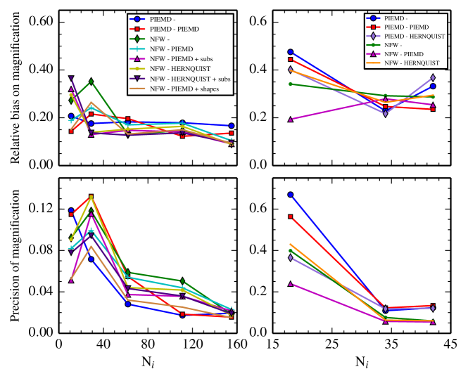
Bottom panels: Relative precision on the magnification measurements as a function of the increasing number of multiple images. Left: Ares. Right: Hera.
5.1 Statistical quality assessment
We use several statistical estimators to assess the quality of each reconstruction: the logarithm of the Likelihood, the RMS (in arcseconds) in the image plane, the reduced , the logarithm of the Evidence and the Bayesian Information Criterion (following Lagattuta
et al., 2016).
The results are summarized in Table 2 and Table 3 for Ares and Hera respectively.
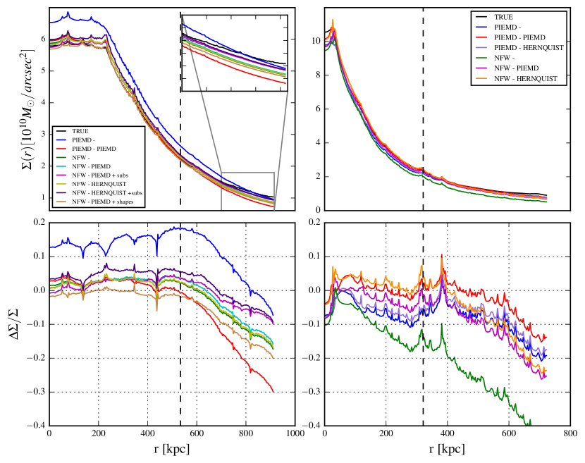
We would like to draw the reader’s attention to the fact that all estimators are consistent with each other but using the logarithm of the Evidence appears to be a better way to differentiate between models. On the other hand, the RMS does not necessarily reflect the improvement of the reconstruction. However, both the BIC and AICc strongly penalize models including the distant substructures in the modelling. Indeed, the greater number of free parameters in these models would not be justified be even though they improve the mass distribution at large radii as well as tighten the cosmological constraints (see Figures 2 and 6, respectively).
As expected, in the case of Ares, considering a NFW profile for the large-scale potentials improves the modelling and Model 7 (NFW - HERNQUIST + subs) gives the best fit for this cluster as it is the closest to the true mass distribution. We show that taking into account the substructures in the cluster’s outskirts for Ares leads to an improvement in the modelling of . Wide field imaging around strong lenses is thus crucial in order to detect such structures and include them in future reconstructions.
For the model NFW-PIEMD + shapes, we see that this additional information worsens the modelling of Ares with a lower value of than the model without. This is in agreement with the true model as input cluster galaxies are spherical (Meneghetti
et al., 2016) thus showing that our modelling technique is sensitive to the shapes of cluster members.
As for Hera, the resulting fit is similar for all models. As expected, the reduced values are larger than those for Ares, as the latter was modelled parametrically (assuming that light traces mass) thus better suited for our modelling technique.
| Model | log(Likelihood) | RMS(") | Reduced | log(Evidence) | BIC | AICc | ||
|---|---|---|---|---|---|---|---|---|
| PIEMD - no BCGs | 76.61 | 1.80 | 1.27 | 33.51 | -15.23 | -24.44 | ||
| PIEMD - PIEMD | 117.00 | 0.66 | 0.81 | 61.46 | -32.77 | -37.93 | ||
| NFW - no BCGs | 144.83 | 0.60 | 0.61 | 95.78 | -163.17 | -97.35 | ||
| NFW - PIEMD | 155.28 | 0.73 | 0.58 | 100.70 | -109.33 | -83.76 | ||
| NFW - PIEMD + SUBS | 166.53 | 0.55 | 0.48 | 107.65 | -45.59 | -47.14 | ||
| NFW - HERNQUIST | 145.54 | 0.58 | 0.61 | 93.58 | -118.59 | -78.97 | ||
| NFW - HERNQUIST + SUBS | 168.31 | 0.64 | 0.50 | 111.43 | -60.65 | -55.69 | ||
| NFW - PIEMD + shapes | 135.56 | 0.57 | 0.65 | 79.82 | -87.14 | -64.04 |
| Model | log(Likelihood) | RMS(") | Reduced | log(Evidence) | BIC | AICc | ||
|---|---|---|---|---|---|---|---|---|
| PIEMD - no BCGs | -35.93 | 0.99 | 2.85 | -77.20 | 207.51 | 126.42 | ||
| PIEMD - PIEMD | -19.44 | 1.21 | 2.64 | -64.97 | 210.71 | 151.36 | ||
| PIEMD - HERNQUIST | -31.80 | 0.96 | 2.98 | -71.60 | 226.38 | 152.24 | ||
| NFW - no BCGs | -43.44 | 0.98 | 2.71 | -79.81 | 222.53 | 133.93 | ||
| NFW - PIEMD | -46.47 | 1.00 | 3.03 | -85.40 | 264.77 | 178.39 | ||
| NFW - HERNQUIST | -44.59 | 0.99 | 2.96 | -81.40 | 251.96 | 165.02 |
5.2 Density profiles
In this section we present the comparison between the radial density profile for all of our models and the true one.
In order to compare our projected mass maps to the input convergence map (with sources assumed at =9), the latter is normalised by multiplying the value of every pixel by (at , and assuming the input cosmology) in order to have the associated surface mass density as:
| (9) |
where:
| (10) |
with , the speed of light, the Newtonian constant and and the angular diameter distances between observer-source, observer-lens and source-lens, respectively.
Our maps and the true one have the same field of view and spatial resolution.
For each model of Section 4, we compute the radial density profile and compare it to the true profile in Figure 2.
-
1.
Ares:
Regardless of the profile used for the large-scale potentials and BCGs, the mass distribution is well constrained within inside the radius below which there are constraints-defined as the radius of the circle enclosing all multiple images (except for the model PIEMD, which is overestimating the cluster’s density by ). However, the density profile in the outskirts of the Ares cluster (beyond the black vertical dashed line, representing the radius containing multiple images) tends to be underestimated by up to . Including the substructures in the modelling helps to better constrain the mass distribution, with an improvement between to in the most distant regions of the cluster. On average, the statistical error is about of the signal for all models, although for Model 1 (PIEMD), it varies from in the inner regions to up to in the outskirts.
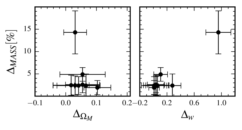
We also display in Figure 3 the bias on the estimation of and (i.e the absolute error between the true value and the mode of the distribution for each of our models, see Figure 6) depending on the bias on the total mass (inside the radius below which there are multiple images) for all of our models of Section 4.1 for Ares (as the constraints on for Hera in Figure 7 are too wide to draw any conclusion). As expected the larger the bias on the mass is, the larger the bias on the cosmological parameters. The bias on the mass is therefore a cosmological quality estimator. Also we show that the equation of state parameter is more affected by a larger bias on the cluster mass than . This result is in agreement with Golse et al. (2002) where the authors showed that the matter density parameter can be better constrained than for a set of simple mock strong lenses. In this work we confirm that is less sensitive to the modelling than , even for more complex clusters such as Ares. -
2.
Hera:
As expected, Hera is less constrained inside the radius below which there are multiple images (within ) and the density profile at the very core of the cluster differs significantly from the true distribution. The density profile is well constrained by all models up to the radius containing multiple images. In the outskirts of the cluster, the density profile differs from the true distribution from up to depending on the model. The statistical error is larger than for Ares, especially for models 3, 4 and 6 , for which it varies from in the center up to in the outskirts.
5.3 Relative bias on magnification
In this section, we detail how we compute the magnifications from our lens models and compare them to the true values.
If we consider sources smaller than the angular scale on which the lens properties change, the Jacobian matrix describing the distortion (in shape and size) of images is then:
| (11) |
where is the convergence and , the first and second shear components respectively. The magnification is then the inverse of the determinant of :
| (12) |
where is the magnification of the source.
-
1.
True magnification
To obtain the true magnification for each multiple image we use the true convergence and shear maps at at any location in the image plane covering a field of view of for Ares and for Hera.
However, to have the true magnification at the source’s redshift, we multiply the true convergence and shear components , by a normalizing factor:(13) Finally, we interpolate this map to get the magnification at the position of all input multiple images.
- 2.
We are interested in how the measured magnification evolves with an increasing number of multiple images.
To do so, we run SExtractor (Bertin &
Arnouts, 1996) to extract and measure the magnitudes on the F814W image (deeper thus more arcs detected) of all the multiple images which are then divided into five different catalogues with increasing magnitude thresholds in the F814W filter (being uniformly distributed in the field).
We then run each lens model presented in Sections 4.1 and 4.2 with all of the new multiple image catalogues (with different magnitude thresholds). We compute the relative bias on magnification per multiple image as well as the 25-th and 75-th percentiles of this distribution. Finally for each magnitude catalogue we compute an average bias on the magnification with:
| (14) |
where is the mode of the magnification distribution per catalogue.
We show in Figure 4 the relative bias on magnification as a function of the number of images taken into account in the modelling for both clusters (top panel) and the precision of our measurements (bottom panel). The bias on the magnification is of the order of for Ares. This bias can go up to for the smallest bins. The magnifications of the multiple images in Hera are less constrained with an average bias of . The relative bias on magnification is not reduced by an increasing number of constraints for either of the clusters. However, the precision on magnification improves by a factor when increasing the constraints in the modelling as stated in Jauzac
et al. (2014). All models provide similar measurements of the magnification and modelling galaxy clusters in a more complex way is not translated into an improvement in the accuracy or precision of magnification.
Taking into account the substructures in the cluster’s outskirts leads to a very localised improvement of the magnification bias of but remains constant within the cluster’s core.
5.4 Cluster ellipticity and orientation
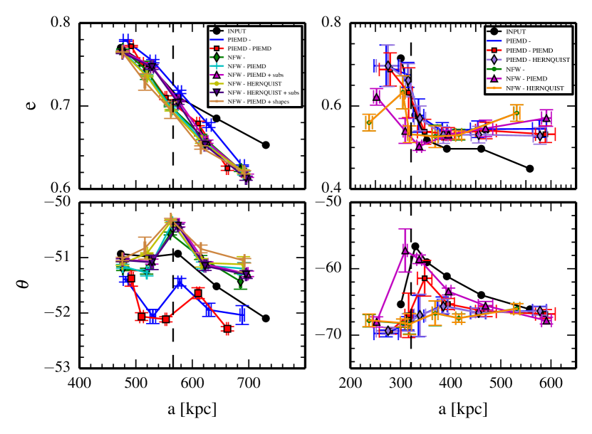
We use the mass maps generated for each model and the normalised true convergence map (as explained in 5.2) to compute the cluster ellipticity as a function of the major semi-axis and its position angle for each model of Section 4.
We set a list of iso-surface density thresholds to fit an ellipse to each contour. As both clusters are bimodal, the highest iso-density contour is set to be the one that encloses both clumps.
The ellipticity is then computed as follows:
| (15) |
where a and b are the measured major and minor semi-axes respectively.
The radial profiles of the ellipticity and of the orientation angle for both clusters are shown in Figure 5.
For each panel the true values are given by the black line. Overall, the values of all the models are in good agreement with the true value in the inner regions (before the dashed vertical line, representing the radius up to where we have multiple images) but tend to differ in the outskirts as our models do not have constraints anymore, thus extrapolating from the core region. The ellipticity in the outskirts of Ares is underestimated but overestimated for Hera. The values of the cluster’s orientation angle are recovered within 5 degrees for Ares and within 10 degrees for Hera.
This estimator does not allow to discriminate between the different models as all models are in perfect agreement.
6 Cosmography
In this section we investigate the impact of considering different cluster modellings on the estimation of cosmological parameters.
We assess first if the choice of different density profiles for the cluster components (large-scale potentials and BCGs) has a significant impact on constraining the and parameter space.
We also analyse the systematic error introduced when using different redshift catalogues for the background sources (spectroscopic only, spectroscopy and photometry) for the lens modelling.
6.1 Estimation of and
As mentioned before, for each model we have (taking into account all multiple images with spectroscopic redshifts), the cosmological parameters and are left as free parameters.
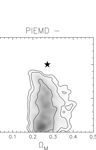
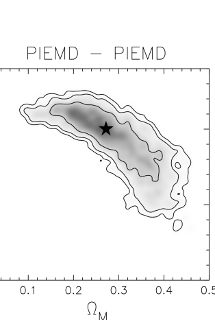
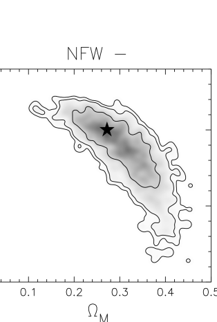
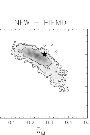
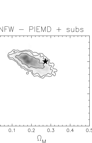
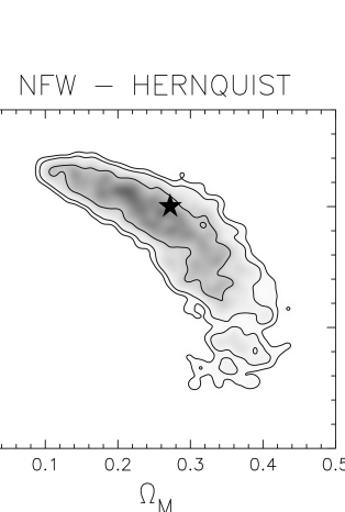
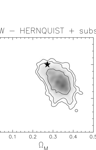
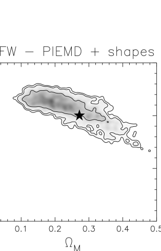
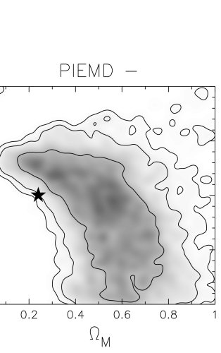
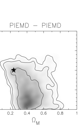
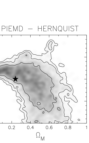
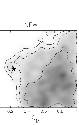
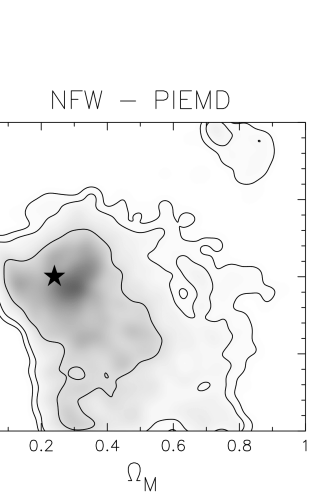
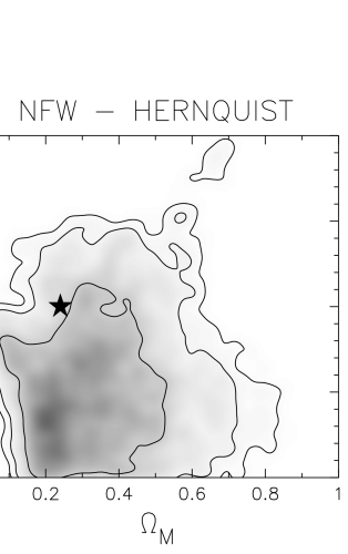
The constraints obtained are shown in Figure 6 for Ares and Figure 7 for Hera.
Using either different density profiles for the large-scale clumps and BCGs provides similar constraints on the and parameter-space (within the 1 contours) if a large number of multiple images is available (with spectroscopic redshifts and with a positional error of 0.5") and if the model is realistic enough (all but model 1: PIEMD,which has the largest mass bias in Figure 3).
However, including in the modelling massive substructures in the cluster’s outskirts translates into a decrease of the statistical errors as the cosmological contours are smaller: at the risk of biasing the results. Our work is in agreement with these previous studies showing that massive structures in the outskirts of clusters do impact, not only the mass distribution but also the constraints on cosmological parameters yielding smaller contours. Not only do the line-of-sight structures introduce a systematic error in the strong lensing modelling (eg. Bayliss et al., 2014; Giocoli
et al., 2016) but also distant massive structures in the lens plane have a considerable impact in the position of multiple images (Tu et al., 2008; Limousin
et al., 2010) and thus on the mass constraints. Indeed, in Mahler
et al. (2017) the authors evaluate the impact of the presence of mass clumps in the outskirts of the cluster core of Abell 2744 (Jauzac
et al., 2016) to change the mass profile by at 200kpc. McCully et al. (2017) have shown that considering the environmental and line of sight perturbations should not be taken aside in the modelling as in doing so, the fit does not reproduce the input lens system parameters or the Hubble constant.
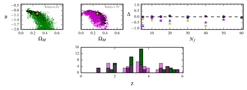
The contours obtained with Hera are, in general, much larger than those from Ares. This can be explained by the fact that the redshift range of Ares’s sources is twice larger than for Hera. By running one of Ares models with multiple images only up to , we checked that, the contours were larger indeed.
The widening of the contours might then not be due to the number of images taken into account as seen in Figure 9. The left panels show the constraints on the - parameter space for one of Ares configurations. Considering the same number of multiple images, but spanning a twice larger range of redshift, provides tighter constraints than those obtained with Hera.
Finally, we would like to point out that recovering cosmological parameters with strong lenses has been until now performed for unimodal clusters (or more simple clusters than the FF) which would be the preferred configuration for cosmography. Recently, Caminha
et al. (2016) performed the first cosmography analysis with a Frontier Fields cluster, AS1063, which is the most relaxed cluster of the sample. By carefully selecting a sub-sample of secured multiple images they achieve a rms of and put constraints on the , and parameters.
However, we show in this work that complex and multimodal clusters such as Ares can yield tight and competitive constraints on the - parameter space.
6.2 Redshift catalogues
In this section we investigate how the estimation of robust cosmological parameters is affected by the availability of different sets of constraints. We extend this study for three of the models for Ares in Section 4.1 (models 2, 3, 6).
These analyses have been only carried out for the Ares cluster as it has three times more multiple images (see Table 1) and the range of redshift is twice wider than for Hera.
6.2.1 Redshift range
We investigate first whether there is a redshift range of background sources more efficient to recover the input cosmology and if photometric redshifts can complete our samples.
We split the redshift catalogue into four bins of redshift:
Bin1 as ,
Bin2 as ,
Bin3 as ,
Bin4 as .
and we build the new multiple images catalogues as follows:
for each of the new four multiple images catalogue we keep the images whose redshift is inside each bin as spectroscopic and the rest as photometric redshifts which have been virtually created with a precision of and assuming there are no catastrophic errors. This precision is already achievable with the HFF data: Castellano
et al. (2016) determined a typical photometric redshift error on the multiple images in Abell 2744 and MACS 0416 of .
Of the 242 total images provided we keep 60 with spectroscopic information per bin and the rest with photometric accuracy.
We also study if it is preferable to only use spectroscopic information or add photometric redshifts as constraints so we also use multiple images catalogues with only images belonging to each bin (having then 60 images, with spectroscopy).
We compare, for each bin of redshift stated above, the constraints on the - parameter-space with photometric redshifts as additional information or not.
The results are shown in Figure 8. For reference, the fiducial models of Figure 6 are also shown (black constraints). First, we show that considering only spectroscopic redshifts from a certain redshift range (blue points) biases the estimation of cosmological parameters whatever the redshift bin considered is, the bias being similar whichever the profile and/or configuration used are for the same bin considered.
By completing these spectroscopic redshifts catalogues with multiple images with photometric information (red points), spanning the ranges in redshift not covered by them, we recover unbiased cosmology (golden star) in most cases or at least reduce this bias. Note that, if cosmological parameters are still biased, it is the equation of state parameter which is more affected than .
Photometric redshifts are then a useful piece of additional information to take into account in the modelling and completing the spectroscopic catalogue if the latter covers only a narrow redshift range.


6.2.2 Photometric families
Considering multiple images from a restricted range of redshift leads to an estimation of wider constraints (which are biased) on the and parameter space whatever the mass distribution of the cluster is. This bias is due to the narrow range of redshifts considered and not to a reduced number of multiple images considered as seen below.
In this section, we consider as constraints a reduced catalogue of multiple images with spectroscopic redshifts by creating two similar catalogues (but with a different redshift distribution) which contain 60 images and spanning all the redshift range available (see histograms in Figure 9). We have considered the same three mass models (id 2, 3 and 6) of Section 4.1 for Ares. For clarity, we only show the results obtained for one of them in Figure 9 as the results were very similar for the 3 of them.
In the left and middle panels we show in black the constraints obtained with the fiducial model NFW- HERNQUIST of (Section 6), on top are the constraints with the two reduced catalogues. As we can notice, the cosmological parameters are unbiased.
We investigate if adding an increasing number of families of multiple images with photometric redshifts (spanning all the redshift range) in the modelling translates into an improvement in the cosmology estimation (i.e a smaller systematic than statistical error). This is shown in the right panels of Figure 9 where the systematic and statistical errors (errors bars) are plotted as a function of the increasing number of photometric families taken in account. The coloured circles show the bias on , the triangles on . We observe the same behaviour for the three models, where is less affected by than the modelling and the statistical errors are smaller than the systematic uncertainties. is systematically underestimated. We do not report, however, any trend with the increasing number of photometric families.
6.3 On the positional uncertainty of the multiple images
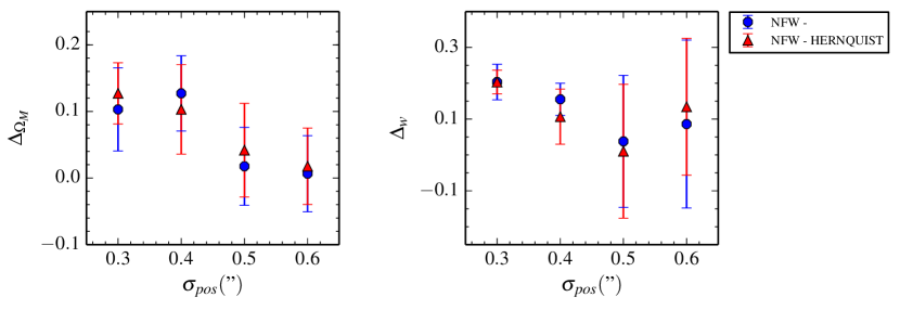
Throughout this paper, we have assumed an uncertainty of 0.5" for the position of multiple images, closer value to the RMS in the image plane thus providing a reduced . We show in Figure 10 the bias on the estimation of and for three positional errors of the multiple images assumed in the modelling for two models of Section 4.1 for Ares. This bias is the lowest for a positional uncertainty of the order of the RMS. However, this Figure also shows that underestimating the uncertainties on the observations can lead to biased constraints on the - parameter space.
7 Conclusions
We have analysed two mock galaxy clusters, Ares and Hera from the FF-SIMS Challenge (Meneghetti
et al., 2016), both complex and bi-modal, comparable to the FF clusters. We have investigated the systematic errors in the strong lensing parametric modelling arising from the choice of the density profiles and configurations as well as from the availability of constraints (spectroscopic or photometric redshifts) and therefore the impact on the retrieval of robust cosmological parameters.
Our main conclusions are the following:
-
1.
Galaxy clusters are not isolated systems and can present large structures in the cluster outskirts (Jauzac et al., 2016; Foëx et al., 2017). With this work we provide further evidence that distant massive substructures in the lens-plane of galaxy clusters have a significant impact on the mass distribution. Wide-field imaging around massive clusters is thus needed to account for these structures in the modelling. In an era of precise cosmology, we show that the cluster’s environment cannot be ignored in order to yield a more precise mass reconstruction and therefore competitive constraints on and .
-
2.
As expected, the smaller the bias on the mass, the smaller the bias on cosmological parameters. The bias on the total mass is a quality indicator for the cosmological constraints. On the other hand, magnification, the cluster’s ellipticity and orientation do not allow to discriminate between models (assuming the same modelling technique).
-
3.
Considering a positional error of , the estimation of cosmological parameters is not affected by the choice of different mass profiles or configurations when a sufficient number of constraints is available ().
-
4.
The bias on the estimation of cosmological parameters is the lowest for a positional uncertainty of the order of the RMS. Underestimating the uncertainty on the observations can lead to biased constraints on the - parameter space.
-
5.
Considering multiple images, from a restricted range of redshift leads to an estimation of biased cosmological parameters. Taking into account multiple images from a broader range of redshift with photometry information can correct this bias or, at least, reduce it.
-
6.
We do not report any trend between an increasing number of photometric families taken into account in the modelling and a more precise estimation of and .
-
7.
is less sensitive to systematic errors than this latter being systematically underestimated when recovered biased.
Stronger constraints can be obtained by combining the estimates on and from several strong lensing clusters (D’Aloisio & Natarajan, 2011). We show that, not only unimodal (or simpler clusters than Ares and Hera; Jullo et al., 2010; Caminha et al., 2016), but also more complex and multimodal clusters can yield competitive constraints. Upcoming surveys such as James Webb Space Telescope will make strong lensing cosmography a very powerful tool by detecting an even larger number of arcs than currently with HST.
Acknowledgments
We thank the referee for her/his useful comments that helped improving this work.
A.A is grateful to Gabriel Bartosch Caminha for useful and constructive discussions. We also thank M. Meneghetti, P. Natarajan and D. Coe for providing the Ares and Hera mock clusters for the Frontier Fields Lens Modeling Comparison Project.
This work has been carried out thanks to the support of the OCEVU Labex (ANR-11-LABX-0060) and the A*MIDEX project (ANR-11-IDEX-0001-02) funded by the "Investissements d’Avenir" French government program managed by the ANR.
This work was granted access to the HPC resources of Aix-Marseille Université financed by the project Equip@Meso (ANR-10-EQPX-29-01) of the program "Investissements d’Avenir" supervised by the Agence Nationale pour la Recherche.
We are also grateful to CNES for financial support. M. L thanks CNRS for financial support.
CG acknowledges support from the Italian Ministry for Education, University and Research (MIUR) through the SIR individual grant SIMCODE, project number RBSI14P4IH
M.J acknowledges support by the Science and Technology Facilities Council [grant number ST/L00075X/1].
References
- Atek et al. (2015) Atek H., et al., 2015, ApJ, 814, 69
- Bayliss et al. (2014) Bayliss M. B., Johnson T., Gladders M. D., Sharon K., Oguri M., 2014, ApJ, 783, 41
- Bayliss et al. (2015) Bayliss M. B., Sharon K., Johnson T., 2015, ApJ, 802, L9
- Bertin & Arnouts (1996) Bertin E., Arnouts S., 1996, A&AS, 117, 393
- Beutler et al. (2011) Beutler F., et al., 2011, MNRAS, 416, 3017
- Bouwens et al. (2016) Bouwens R. J., Oesch P. A., Illingworth G. D., Ellis R. S., Stefanon M., 2016, preprint, (arXiv:1610.00283)
- Caminha et al. (2016) Caminha G. B., et al., 2016, A&A, 587, A80
- Castellano et al. (2016) Castellano M., et al., 2016, A&A, 590, A31
- Coe et al. (2006) Coe D., Benítez N., Sánchez S. F., Jee M., Bouwens R., Ford H., 2006, AJ, 132, 926
- Coe et al. (2013) Coe D., et al., 2013, ApJ, 762, 32
- D’Aloisio & Natarajan (2011) D’Aloisio A., Natarajan P., 2011, MNRAS, 411, 1628
- Dalal et al. (2005) Dalal N., Hennawi J. F., Bode P., 2005, ApJ, 622, 99
- De Lucia & Blaizot (2007) De Lucia G., Blaizot J., 2007, MNRAS, 375, 2
- Despali et al. (2017) Despali G., Giocoli C., Bonamigo M., Limousin M., Tormen G., 2017, MNRAS, 466, 181
- Diego et al. (2016) Diego J. M., Broadhurst T., Wong J., Silk J., Lim J., Zheng W., Lam D., Ford H., 2016, MNRAS, 459, 3447
- Faber & Jackson (1976) Faber S. M., Jackson R. E., 1976, ApJ, 204, 668
- Foëx et al. (2017) Foëx G., Chon G., Böhringer H., 2017, preprint, (arXiv:1703.02763)
- Gil-Marín et al. (2016) Gil-Marín H., et al., 2016, MNRAS, 460, 4210
- Gilmore & Natarajan (2009) Gilmore J., Natarajan P., 2009, MNRAS, 396, 354
- Giocoli et al. (2012) Giocoli C., Meneghetti M., Bartelmann M., Moscardini L., Boldrin M., 2012, MNRAS, 421, 3343
- Giocoli et al. (2014) Giocoli C., Meneghetti M., Metcalf R. B., Ettori S., Moscardini L., 2014, MNRAS, 440, 1899
- Giocoli et al. (2016) Giocoli C., Bonamigo M., Limousin M., Meneghetti M., Moscardini L., Angulo R. E., Despali G., Jullo E., 2016, MNRAS, 462, 167
- Golse & Kneib (2002) Golse G., Kneib J.-P., 2002, A&A, 390, 821
- Golse et al. (2002) Golse G., Kneib J.-P., Soucail G., 2002, A&A, 387, 788
- Harvey et al. (2016) Harvey D., Kneib J. P., Jauzac M., 2016, MNRAS, 458, 660
- Hernquist (1990) Hernquist L., 1990, ApJ, 356, 359
- Heymans et al. (2012) Heymans C., et al., 2012, MNRAS, 427, 146
- Hildebrandt et al. (2017) Hildebrandt H., et al., 2017, MNRAS, 465, 1454
- Host (2012) Host O., 2012, MNRAS, 420, L18
- Jauzac et al. (2014) Jauzac M., et al., 2014, MNRAS, 443, 1549
- Jauzac et al. (2016) Jauzac M., et al., 2016, MNRAS, 463, 3876
- Johnson & Sharon (2016) Johnson T. L., Sharon K., 2016, ApJ, 832, 82
- Jullo et al. (2007) Jullo E., Kneib J.-P., Limousin M., Elíasdóttir Á., Marshall P. J., Verdugo T., 2007, New Journal of Physics, 9, 447
- Jullo et al. (2010) Jullo E., Natarajan P., Kneib J.-P., D’Aloisio A., Limousin M., Richard J., Schimd C., 2010, Science, 329, 924
- Kassiola & Kovner (1993) Kassiola A., Kovner I., 1993, ApJ, 417, 450
- Kneib et al. (1996) Kneib J.-P., Ellis R. S., Smail I., Couch W. J., Sharples R. M., 1996, ApJ, 471, 643
- Kneib et al. (2004) Kneib J.-P., Ellis R. S., Santos M. R., Richard J., 2004, ApJ, 607, 697
- Lagattuta et al. (2016) Lagattuta D. J., et al., 2016, preprint, (arXiv:1611.01513)
- Limousin et al. (2005) Limousin M., Kneib J.-P., Natarajan P., 2005, MNRAS, 356, 309
- Limousin et al. (2010) Limousin M., et al., 2010, A&A, 524, A95
- Limousin et al. (2016) Limousin M., et al., 2016, A&A, 588, A99
- Link & Pierce (1998) Link R., Pierce M. J., 1998, ApJ, 502, 63
- Lotz et al. (2017) Lotz J. M., et al., 2017, ApJ, 837, 97
- Magaña et al. (2015) Magaña J., Motta V., Cardenas V. H., Verdugo T., Jullo E., 2015, Astrophys. J., 813, 69
- Mahler et al. (2017) Mahler G., et al., 2017, preprint, (arXiv:1702.06962)
- Massey et al. (2007) Massey R., et al., 2007, ApJS, 172, 239
- McCully et al. (2017) McCully C., Keeton C. R., Wong K. C., Zabludoff A. I., 2017, ApJ, 836, 141
- Meneghetti et al. (2008) Meneghetti M., et al., 2008, A&A, 482, 403
- Meneghetti et al. (2010) Meneghetti M., Fedeli C., Pace F., Gottlöber S., Yepes G., 2010, A&A, 519, A90
- Meneghetti et al. (2016) Meneghetti M., et al., 2016, preprint, (arXiv:1606.04548)
- Monna et al. (2017) Monna A., et al., 2017, MNRAS,
- Navarro et al. (1997) Navarro J. F., Frenk C. S., White S. D. M., 1997, ApJ, 490, 493
- Newman et al. (2013) Newman A. B., Treu T., Ellis R. S., Sand D. J., 2013, ApJ, 765, 25
- Peel et al. (2017) Peel A., Lin C.-A., Lanusse F., Leonard A., Starck J.-L., Kilbinger M., 2017, in American Astronomical Society Meeting Abstracts. p. 430.01
- Planck Collaboration et al. (2016a) Planck Collaboration et al., 2016a, A&A, 594, A13
- Planck Collaboration et al. (2016b) Planck Collaboration et al., 2016b, A&A, 594, A14
- Planelles et al. (2014) Planelles S., Borgani S., Fabjan D., Killedar M., Murante G., Granato G. L., Ragone-Figueroa C., Dolag K., 2014, MNRAS, 438, 195
- Richard et al. (2008) Richard J., Stark D. P., Ellis R. S., George M. R., Egami E., Kneib J.-P., Smith G. P., 2008, ApJ, 685, 705
- Richard et al. (2010) Richard J., Kneib J.-P., Limousin M., Edge A., Jullo E., 2010, MNRAS, 402, L44
- Riess et al. (1998) Riess A. G., et al., 1998, AJ, 116, 1009
- Schwarz (1978) Schwarz G., 1978, Annals of Statistics, 6, 461
- Sereno et al. (2015) Sereno M., Giocoli C., Ettori S., Moscardini L., 2015, MNRAS, 449, 2024
- Soucail et al. (2004) Soucail G., Kneib J.-P., Golse G., 2004, A&A, 417, L33
- Suyu et al. (2016) Suyu S. H., et al., 2016, preprint, (arXiv:1607.00017)
- Tu et al. (2008) Tu H., Limousin M., Fort B., Shu C. G., Sygnet J. F., Jullo E., Kneib J. P., Richard J., 2008, MNRAS, 386, 1169
- Wang et al. (2006) Wang L., Li C., Kauffmann G., De Lucia G., 2006, MNRAS, 371, 537
- Zitrin & Broadhurst (2016) Zitrin A., Broadhurst T., 2016, ApJ, 833, 25
- Zitrin et al. (2015) Zitrin A., et al., 2015, ApJ, 801, 44
- de Haan et al. (2016) de Haan T., et al., 2016, preprint, (arXiv:1603.06522)
Appendix A Source redshift distribution
We show in Figure 11 the redshift distribution of background sources for the Ares and Hera clusters
