On Information Transfer in Control Dynamical Systems

Subhrajit Sinha and Umesh Vaidya
Financial support from the National Science Foundation grant ECCS-1150405 and CNS-1329915 is gratefully acknowledged. S. Sinha and U. Vaidya is with the Department of Electrical & Computer Engineering, Iowa State University, Ames, IA 50011 ugvaidya@iastate.edu
Abstract

In this paper, we show through examples, how the existing definitions of information transfer, namely directed information and transfer entropy fail to capture true causal interaction between states in control dynamical system. We propose a new definition of information transfer, based on the ideas from dynamical system theory, and show that this new definition can capture true causal interaction between states. The information transfer measure is generalized to define transfers between the various signals in a control dynamical system and analytical expression for information transfer between state-to-state, input-to-state, state-to-output, and input-to-output are provided for linear systems. There is a natural extension of our proposed definition to define information transfer over n𝑛n time steps and average information transfer over infinite time step. We show that the average information transfer in feedback control system between plant output and input is equal to the entropy of the open loop dynamics thereby re-deriving the Bode fundamental limitation results using the proposed definition of transfer.

1 Introduction

From the days of Aristotle, philosophers and scientists have been concerned with the notion of causality. As far back as 300 B.C. Aristotle had realized the importance of causality and even after about two and half thousand years, there is no universally accepted definition of causality. But causality and influence characterization is a subject of immense importance and finds its application in many different applications like world wide web and social media, biological networks, neural science, economics, finance etc. Usually, concepts of information theory are used in such applications and a study of the information flow between the components of the network throws light on causality and the influential nodes of the network. In [1] the authors use information based metric to characterize the most influential nodes in social networks. In neuroscience, concepts of information theory are used to understand how information flows in different parts of the brain [2] and identifying influence in gene regulatory networks [3, 4] . In economic and financial networks, information transfer can be used to infer causal interactions from the time series data [5, 6, 7]. In control theoretic setting, in [8], the authors have used information theoretic ideas to study the classical concepts of control like controllability and observability.

Causality characterization was initially geared towards time series data and Granger causality [5],[7], directed information [9],[10] and Schreiber’s transfer entropy [11] have been the most popular tools used for inferring the causality structure and influence characterization. In dynamical system setting, it was Liang and Kleeman [12],[13] who introduced the concept of information transfer between the states and used it for predictability analysis.

The formulation of information transfer used in this paper is in dynamical systems setting and is closely related to and inspired from information transfer framework developed in [14, 12, 15] for nonlinear dynamical systems. We used the ideas of Liang-Kleeman transfer to propose an axiomatic definition of information transfer in discrete linear dynamic network [16]. The axioms were physically motivated and it was shown in [16] that there exists a unique expression for information transfer in a dynamic network satisfying these axioms. In [16], we had used absolute entropy to characterize the information flow. However, motivated by the definitions of directed information and transfer entropy, in this work we use conditional entropy instead of absolute entropy to characterize the information flow.

Motivation for this work lies in the fact that, in dynamical systems, directed information fails to capture the intuitions of information transfer, and thus provide erroneous conclusion about the causal structure in a dynamical system. We show that our definition of information transfer does capture the correct causal structure of the system. We show, how this definition of information transfer between the states of a dynamical system can be easily extended to study the the information transfer between the inputs and outputs in a control dynamical system. In fact, this natural extension leads us to connect the information transfer to the Bode integral of the sensitivity transfer function from the output to the input in a feedback control system.

The paper is organised as follows. In section 2, we discuss, through some examples, how directed information fails to capture the notions of causality (zero transfer and indirect influence). In section 3 we provide our definition of information transfer. We also define n𝑛n-step information transfer and average information transfer and for linear systems, we provide explicit formulas for computing the transfer. We also revisit the examples in section 2 and show how our definition of information transfer captures the intuitions of information transfer. In section 4, we generalize our definition of information transfer to define information transfer between the inputs and outputs in a linear control dynamical system. We also study the information transfer in a feedback control system and show how this is related to the Bode integral of the sensitivity transfer function from the output to the input. This is followed by conclusions in section 6.

2 Directed Information as a Measure of Causality

Directed information and transfer entropy are two of the most popular notions of information transfer used to characterize causality. In this section, we show that these notions of information transfer cannot faithfully capture the true causality structure in control dynamical system.

Directed information was first defined by Massey [9] as a generalization of Marko’s bidirectional information [17]. Both bidirectional information and directed information gave a sense of direction to Shannon’s information theory and is viewed as a generalized information theory. Let Xn={X1,X2,,Xn}superscript𝑋𝑛subscript𝑋1subscript𝑋2subscript𝑋𝑛X^{n}=\{X_{1},X_{2},\cdots,X_{n}\} and Yn={Y1,Y2,,Yn}superscript𝑌𝑛subscript𝑌1subscript𝑌2subscript𝑌𝑛Y^{n}=\{Y_{1},Y_{2},\cdots,Y_{n}\} be two stochastic processes, viewed as a sequence of random variables. Massey and Kramer [10] defined the directed information from Xnsuperscript𝑋𝑛X^{n} to Ynsuperscript𝑌𝑛Y^{n} as

I(XnYn)=H(Yn)H(YnXn)𝐼superscript𝑋𝑛superscript𝑌𝑛𝐻superscript𝑌𝑛𝐻conditionalsuperscript𝑌𝑛superscript𝑋𝑛\displaystyle I(X^{n}\to Y^{n})=H(Y^{n})-H(Y^{n}\parallel X^{n}) (1)

where H(Yn)𝐻superscript𝑌𝑛H(Y^{n}) is the entropy of the sequence Ynsuperscript𝑌𝑛Y^{n} and H(YnXn):=i=1nH(Yi|Yi1,Xi)assign𝐻conditionalsuperscript𝑌𝑛superscript𝑋𝑛superscriptsubscript𝑖1𝑛𝐻conditionalsubscript𝑌𝑖superscript𝑌𝑖1superscript𝑋𝑖H(Y^{n}\parallel X^{n}):=\sum_{i=1}^{n}H(Y_{i}|Y^{i-1},X^{i}) is the entropy of Ynsuperscript𝑌𝑛Y^{n} causally conditioned on Xnsuperscript𝑋𝑛X^{n}.

The directed information is asymmetric and gives a directional sense to the information and defines a measure to determine the direction of information flow. Since the development of the concept of directed information, this has been used in many different applications, like determining the channel capacity of a communication channel. Moreover, for Gaussian variables, directed information and Granger causality [7], [5] are equivalent [18]. This allows the concept of directed information to be used as a measure of causality and hence it has been used to infer about the causal structure of statistical processes. In the following, we demonstrate using three different examples how the directed information fails to capture the true causality structure in dynamical systems setting. While the arguments are made in the context of directed information, similar conclusions can be drawn in the context of transfer entropy. We claim that at the heart of the problem is the manner in which causal conditioning is performed in both these definitions of information transfer.

2.1 Examples

Example 1.

Consider the following linear system with output
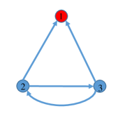
(x1(t+1)x2(t+1)x3(t+1))matrixsubscript𝑥1𝑡1subscript𝑥2𝑡1subscript𝑥3𝑡1\displaystyle\begin{pmatrix}x_{1}(t+1)\\ x_{2}(t+1)\\ x_{3}(t+1)\end{pmatrix} =\displaystyle= (00.50.5000.5010)(x1(t)x2(t)x3(t))+σξ(k)matrix00.50.5000.5010matrixsubscript𝑥1𝑡subscript𝑥2𝑡subscript𝑥3𝑡𝜎𝜉𝑘\displaystyle\begin{pmatrix}0&0.5&0.5\\ 0&0&0.5\\ 0&1&0\end{pmatrix}\begin{pmatrix}x_{1}(t)\\ x_{2}(t)\\ x_{3}(t)\end{pmatrix}+\sigma\xi(k)
Refer to caption
Refer to caption
Figure 1: (a) Graph of dynamical system of example 1. (b) Graph of dynamical system of example 2.

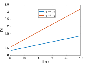
where xi(t)subscript𝑥𝑖𝑡x_{i}(t) are the states at time step t𝑡t and ξ(t)𝜉𝑡\xi(t) is a independent identically distributed (i.i.d.) zero mean unit variance Gaussian noise and σ𝜎\sigma is a constant. We notice that while there is directed path from x2x1subscript𝑥2subscript𝑥1x_{2}\to x_{1} and x3x1subscript𝑥3subscript𝑥1x_{3}\to x_{1} (fig. 1(a)), there is no path from x1subscript𝑥1x_{1} to x2subscript𝑥2x_{2} or from x1subscript𝑥1x_{1} to x3subscript𝑥3x_{3}. Hence, we conclude that x1subscript𝑥1x_{1} is not a cause of x2subscript𝑥2x_{2} or x3subscript𝑥3x_{3}, that is, x1subscript𝑥1x_{1} is not influencing x2subscript𝑥2x_{2} or x3subscript𝑥3x_{3}. So if we treat the dynamical system as a stochastic process, we expect that the flow of information from x1x2subscript𝑥1subscript𝑥2x_{1}\to x_{2} and x1x3subscript𝑥1subscript𝑥3x_{1}\to x_{3} to be zero, thereby inferring that there is no causal connection from x1x2subscript𝑥1subscript𝑥2x_{1}\to x_{2} and x1x3subscript𝑥1subscript𝑥3x_{1}\to x_{3}. In fact closer examination reveals that x1subscript𝑥1x_{1} is not influencing x2subscript𝑥2x_{2} and x3subscript𝑥3x_{3} over any number of time steps. However, as we show below, the directed information fails to capture this true causal interaction between state x1,x2,subscript𝑥1subscript𝑥2x_{1},x_{2}, and x3subscript𝑥3x_{3}. In particular, we show that I(x1nx2n)0𝐼superscriptsubscript𝑥1𝑛superscriptsubscript𝑥2𝑛0I(x_{1}^{n}\to x_{2}^{n})\neq 0 and I(x1nx3n)0𝐼superscriptsubscript𝑥1𝑛superscriptsubscript𝑥3𝑛0I(x_{1}^{n}\to x_{3}^{n})\neq 0 for any n𝑛n. In Fig. 2, we plot the directed information from x1x2subscript𝑥1subscript𝑥2x_{1}\to x_{2} and x1x3subscript𝑥1subscript𝑥3x_{1}\to x_{3} over different time steps.

Refer to caption
Refer to caption
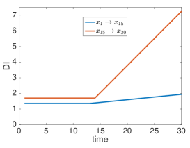
Figure 2: (a) Directed information plots for example 1. (b) Directed information plots for example 2.
Example 2.

Next we consider a single input single output linear system

x(t+1)=(000010000010)x(t)+(100)u𝑥𝑡1matrix000010000010𝑥𝑡matrix100𝑢\displaystyle x(t+1)=\begin{pmatrix}0&0&\ldots&0&0\\ 1&0&\ldots&0&0\\ \vdots&\vdots&\vdots&\ddots&\vdots\\ 0&0&\ldots&1&0\end{pmatrix}x(t)+\begin{pmatrix}1\\ 0\\ \vdots\\ 0\end{pmatrix}u
y(t)=(01)x(t)𝑦𝑡matrix01𝑥𝑡\displaystyle y(t)=\begin{pmatrix}0&\ldots&1\end{pmatrix}x(t) (3)

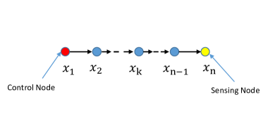
where x(t)N𝑥𝑡superscript𝑁x(t)\in\mathbb{R}^{N}. We note that the state x1subscript𝑥1x_{1} is directly controlled through u𝑢u and measurements are made at state xNsubscript𝑥𝑁x_{N}. State xksubscript𝑥𝑘x_{k}, for 1<<k<<Nmuch-less-than1𝑘much-less-than𝑁1<<k<<N, is assumed to be some intermittent state. Since the control input u𝑢u does not affect state xksubscript𝑥𝑘x_{k} instantaneously, but through series of k𝑘k delays, we expect the information flow from state x1subscript𝑥1x_{1} to xksubscript𝑥𝑘x_{k} to be zero for time step t=0,,k1𝑡0𝑘1t=0,\ldots,k-1. On the other hand since xksubscript𝑥𝑘x_{k} influence xNsubscript𝑥𝑁x_{N} again through series of delay we expect the information flow from xksubscript𝑥𝑘x_{k} to xnsubscript𝑥𝑛x_{n} to zero for t=k,,Nk1𝑡𝑘𝑁𝑘1t=k,\ldots,N-k-1. However as we show in Fig. 2, directed information from x1xksubscript𝑥1subscript𝑥𝑘x_{1}\to x_{k} and xkxNsubscript𝑥𝑘subscript𝑥𝑁x_{k}\to x_{N} is nonzero for all time t=0,,𝑡0t=0,\ldots, conveying that there is instantaneous flow of information from x1subscript𝑥1x_{1} to xksubscript𝑥𝑘x_{k} and from xksubscript𝑥𝑘x_{k} to xNsubscript𝑥𝑁x_{N}. The simulation results in Fig. 2 are obtained for N=30𝑁30N=30 nodes with k=15𝑘15k=15. This example demonstrates that the directed information fails to capture indirect path of influence.

The above examples reveal some serious deficiencies of directed information as a measure of causality in dynamical system setting. This suggest that the directed information is a measure of statistical interaction between two signals but it does not successfully capture the true dynamical interactions between dynamical states. We expect that any meaningful definition of information transfer in network dynamical system be able to capture true causal interaction and also obey time constraint of information flow. Our proposed definition of information transfer discussed in the following section precisely does that.

3 A New Definition of Information Transfer

Consider the following discrete time dynamical system,

z(t+1)=f(z(t))+ξ(t)𝑧𝑡1𝑓𝑧𝑡𝜉𝑡\displaystyle z(t+1)=f(z(t))+\xi(t) (4)

where z(t)N𝑧𝑡superscript𝑁z(t)\in\mathbb{R}^{N}, ξ(t)N𝜉𝑡superscript𝑁\xi(t)\in\mathbb{R}^{N} is assumed to vector valued random variable and ξ(0),ξ(1),𝜉0𝜉1\xi(0),\xi(1),\ldots are independent random vectors each having the same density g𝑔g. The mapping f:NN:𝑓superscript𝑁superscript𝑁f:\mathbb{R}^{N}\to\mathbb{R}^{N} is assumed to be at least continuous. Let z=(z1,,zN)N𝑧superscriptsubscript𝑧1subscript𝑧𝑁topsuperscript𝑁z=(z_{1},\ldots,z_{N})^{\top}\in\mathbb{R}^{N}. We are interested in defining the information transfer from state zisubscript𝑧𝑖z_{i} to state zjsubscript𝑧𝑗z_{j}, as the system evolves from time step t𝑡t to time step t+1𝑡1t+1. We denote this transfer by the notation [Tzizj]tt+1superscriptsubscriptdelimited-[]subscript𝑇subscript𝑧𝑖subscript𝑧𝑗𝑡𝑡1[T_{z_{i}\to z_{j}}]_{t}^{t+1}.

We provide the following definition for information transfer from state zisubscript𝑧𝑖z_{i} to state zjsubscript𝑧𝑗z_{j} for the dynamical system (4) :

Definition 3 (Information transfer).

The information transfer from zisubscript𝑧𝑖z_{i} to zjsubscript𝑧𝑗z_{j} for dynamical system (4) as the system evolves from time t𝑡t to time t+1𝑡1t+1 and denoted by [Tzizj]tt+1superscriptsubscriptdelimited-[]subscript𝑇subscript𝑧𝑖subscript𝑧𝑗𝑡𝑡1[T_{z_{i}\to z_{j}}]_{t}^{t+1} is given by following formula

[Tzizj]tt+1=H(ρ(zj(t+1)|zj(t)))H(ρi(zj(t+1)|zj(t))\displaystyle[T_{z_{i}\to z_{j}}]_{t}^{t+1}=H(\rho(z_{j}(t+1)|z_{j}(t)))-H(\rho_{\not{z}_{i}}(z_{j}(t+1)|z_{j}(t)) (5)

where H(ρ(zj))=|zj|ρ(zj)logρ(zj)𝑑zj𝐻𝜌subscript𝑧𝑗subscriptsuperscriptsubscript𝑧𝑗𝜌subscript𝑧𝑗𝜌subscript𝑧𝑗differential-dsubscript𝑧𝑗H(\rho(z_{j}))=-\int_{\mathbb{R}^{|z_{j}|}}\rho(z_{j})\log\rho(z_{j})dz_{j} is the entropy of probability density function ρ(zj)𝜌subscript𝑧𝑗\rho(z_{j}) and H(ρi(zj(t+1)|zj(t))H(\rho_{\not{z}_{i}}(z_{j}(t+1)|z_{j}(t)) is the entropy of zj(t+1)subscript𝑧𝑗𝑡1z_{j}(t+1), conditioned on zj(t)subscript𝑧𝑗𝑡z_{j}(t), where zisubscript𝑧𝑖z_{i} has been frozen.

The above definition of information transfer can be understood by rewriting the expression of information transfer as follows:

H(ρ(zj(t+1)|zj(t)))=[Tzizj]tt+1+H(ρi(zj(t+1)|zj(t)))𝐻𝜌conditionalsubscript𝑧𝑗𝑡1subscript𝑧𝑗𝑡superscriptsubscriptdelimited-[]subscript𝑇subscript𝑧𝑖subscript𝑧𝑗𝑡𝑡1𝐻subscript𝜌subscriptitalic-z̸𝑖conditionalsubscript𝑧𝑗𝑡1subscript𝑧𝑗𝑡\displaystyle H(\rho(z_{j}(t+1)|z_{j}(t)))=[T_{z_{i}\to z_{j}}]_{t}^{t+1}+H(\rho_{\not{z}_{i}}(z_{j}(t+1)|z_{j}(t))) (6)

so that the total entropy of zjsubscript𝑧𝑗z_{j} is the sum of transfer from zisubscript𝑧𝑖z_{i} and the entropy of zjsubscript𝑧𝑗z_{j}, when zisubscript𝑧𝑖z_{i} is absent.

3.1 n-step Information Transfer

The information transfer defined in (5) gives the information transferred from zisubscript𝑧𝑖z_{i} to zjsubscript𝑧𝑗z_{j} as the dynamical system evolves from time step t𝑡t to time step t+1𝑡1t+1. So one can look at this definition as a one-step transfer. To generalize the one step transfer to n𝑛n-step transfer, we define the n𝑛n-step transfer from zisubscript𝑧𝑖z_{i} to zjsubscript𝑧𝑗z_{j} as the system evolves from time step t𝑡t to t+n𝑡𝑛t+n, where n>0𝑛subscriptabsent0n\in\mathbb{Z}_{>0}, as follows :

Definition 4 (n𝑛n-step Information transfer).

The information transferred over n𝑛n time steps, n>0𝑛subscriptabsent0n\in\mathbb{Z}_{>0}, from zisubscript𝑧𝑖z_{i} to zjsubscript𝑧𝑗z_{j}, which is denoted as (Tzizj)tt+nsuperscriptsubscriptsubscript𝑇subscript𝑧𝑖subscript𝑧𝑗𝑡𝑡𝑛(T_{z_{i}\to z_{j}})_{t}^{t+n}, as the dynamical system (4) evolves from time step t𝑡t to t+n𝑡𝑛t+n, is defined as

(Tzizj)tt+n=H(ρ(zj(t+n)|zj(t+n1)zj(t)))superscriptsubscriptsubscript𝑇subscript𝑧𝑖subscript𝑧𝑗𝑡𝑡𝑛𝐻𝜌conditionalsubscript𝑧𝑗𝑡𝑛subscript𝑧𝑗𝑡𝑛1subscript𝑧𝑗𝑡\displaystyle(T_{z_{i}\to z_{j}})_{t}^{t+n}=H(\rho(z_{j}(t+n)|z_{j}(t+n-1)\cdots z_{j}(t)))
H(ρi(zj(t+n)|zj(t+n1)zj(t)))𝐻subscript𝜌subscriptitalic-z̸𝑖conditionalsubscript𝑧𝑗𝑡𝑛subscript𝑧𝑗𝑡𝑛1subscript𝑧𝑗𝑡\displaystyle\qquad\qquad\qquad-H(\rho_{\not{z}_{i}}(z_{j}(t+n)|z_{j}(t+n-1)\cdots z_{j}(t))) (7)

where H(ρ(zj(t+n)|zj(t+n1)zj(t)))𝐻𝜌conditionalsubscript𝑧𝑗𝑡𝑛subscript𝑧𝑗𝑡𝑛1subscript𝑧𝑗𝑡H(\rho(z_{j}(t+n)|z_{j}(t+n-1)\cdots z_{j}(t))) is the conditional entropy of zj(t+n)subscript𝑧𝑗𝑡𝑛z_{j}(t+n), conditioned on past n𝑛n-steps of zjsubscript𝑧𝑗z_{j} and H(ρi(zj(t+n)|zj(t+n1)zj(t)))𝐻subscript𝜌subscriptitalic-z̸𝑖conditionalsubscript𝑧𝑗𝑡𝑛subscript𝑧𝑗𝑡𝑛1subscript𝑧𝑗𝑡H(\rho_{\not{z}_{i}}(z_{j}(t+n)|z_{j}(t+n-1)\cdots z_{j}(t))) is the conditional entropy of zj(t+n)subscript𝑧𝑗𝑡𝑛z_{j}(t+n) on its past n𝑛n-steps and the state zisubscript𝑧𝑖z_{i} has been frozen (held constant) from time step t𝑡t to time step t+n𝑡𝑛t+n.

In general, we have the following

Theorem 5.
i=1n(Tzizj)tt+i=H(zj(t+n)zj(t))Hi(zj(t+n)zj(t))superscriptsubscript𝑖1𝑛superscriptsubscriptsubscript𝑇subscript𝑧𝑖subscript𝑧𝑗𝑡𝑡𝑖𝐻subscript𝑧𝑗𝑡𝑛subscript𝑧𝑗𝑡subscript𝐻subscriptitalic-z̸𝑖subscript𝑧𝑗𝑡𝑛subscript𝑧𝑗𝑡\displaystyle\sum_{i=1}^{n}(T_{z_{i}\to z_{j}})_{t}^{t+i}=H(z_{j}(t+n)\cdots z_{j}(t))-H_{\not{z}_{i}}(z_{j}(t+n)\cdots z_{j}(t)) (8)

where

H(zj(t+n)zj(t))=H(ρ(zj(t+n)zj(t)))𝐻subscript𝑧𝑗𝑡𝑛subscript𝑧𝑗𝑡𝐻𝜌subscript𝑧𝑗𝑡𝑛subscript𝑧𝑗𝑡\displaystyle H(z_{j}(t+n)\cdots z_{j}(t))=H(\rho(z_{j}(t+n)\cdots z_{j}(t)))

and

Hi(zj(t+n)zj(t))=H(ρi(zj(t+n)zj(t))).subscript𝐻subscriptitalic-z̸𝑖subscript𝑧𝑗𝑡𝑛subscript𝑧𝑗𝑡𝐻subscript𝜌subscriptitalic-z̸𝑖subscript𝑧𝑗𝑡𝑛subscript𝑧𝑗𝑡\displaystyle H_{\not{z}_{i}}(z_{j}(t+n)\cdots z_{j}(t))=H(\rho_{\not{z}_{i}}(z_{j}(t+n)\cdots z_{j}(t))).
Proof.

We prove this by induction. For i=1𝑖1i=1, using the fact that H(y)=H(y)𝐻𝑦subscript𝐻italic-x̸𝑦H(y)=H_{\not{x}}(y), we have (Txy)tt+1=H(y,y)H(y,y)superscriptsubscriptsubscript𝑇𝑥𝑦𝑡𝑡1𝐻superscript𝑦𝑦subscript𝐻italic-x̸superscript𝑦𝑦(T_{x\to y})_{t}^{t+1}=H(y^{\prime},y)-H_{\not{x}}(y^{\prime},y).

Let this be true for i=k𝑖𝑘i=k. Hence, we have,

i=1k(Txy)tt+i=H(y(t+k)y(t))H(y(t+k)y(t))superscriptsubscript𝑖1𝑘superscriptsubscriptsubscript𝑇𝑥𝑦𝑡𝑡𝑖𝐻𝑦𝑡𝑘𝑦𝑡subscript𝐻italic-x̸𝑦𝑡𝑘𝑦𝑡\displaystyle\sum_{i=1}^{k}(T_{x\to y})_{t}^{t+i}=H(y(t+k)\cdots y(t))-H_{\not{x}}(y(t+k)\cdots y(t))

Now,

(Txy)tt+k+1=H(y(t+k+1)|y(t+k)y(t))H(y(t+k+1)|y(t+k)y(t))=[H(y(t+k+1)y(t))H(y(t+k+1)y(t))][H(y(t+k)y(t))H(y(t+k)y(t))]=[H(y(t+k+1)y(t))H(y(t+k+1)y(t))]i=1k(Txy)tt+imissing-subexpressionsuperscriptsubscriptsubscript𝑇𝑥𝑦𝑡𝑡𝑘1𝐻conditional𝑦𝑡𝑘1𝑦𝑡𝑘𝑦𝑡subscript𝐻italic-x̸conditional𝑦𝑡𝑘1𝑦𝑡𝑘𝑦𝑡missing-subexpressionabsentdelimited-[]𝐻𝑦𝑡𝑘1𝑦𝑡subscript𝐻italic-x̸𝑦𝑡𝑘1𝑦𝑡missing-subexpressiondelimited-[]𝐻𝑦𝑡𝑘𝑦𝑡subscript𝐻italic-x̸𝑦𝑡𝑘𝑦𝑡missing-subexpressionabsentdelimited-[]𝐻𝑦𝑡𝑘1𝑦𝑡subscript𝐻italic-x̸𝑦𝑡𝑘1𝑦𝑡superscriptsubscript𝑖1𝑘superscriptsubscriptsubscript𝑇𝑥𝑦𝑡𝑡𝑖\displaystyle\begin{aligned} &(T_{x\to y})_{t}^{t+k+1}=H(y(t+k+1)|y(t+k)\cdots y(t))-H_{\not{x}}(y(t+k+1)|y(t+k)\cdots y(t))\\ &=[H(y(t+k+1)\cdots y(t))-H_{\not{x}}(y(t+k+1)\cdots y(t))]\\ &\quad-[H(y(t+k)\cdots y(t))-H_{\not{x}}(y(t+k)\cdots y(t))]\\ &=[H(y(t+k+1)\cdots y(t))-H_{\not{x}}(y(t+k+1)\cdots y(t))]-\sum_{i=1}^{k}(T_{x\to y})_{t}^{t+i}\end{aligned}

Hence,

i=1k+1(Txy)tt+i=H(y(t+k+1)y(t))H(y(t+k+1)y(t))superscriptsubscript𝑖1𝑘1superscriptsubscriptsubscript𝑇𝑥𝑦𝑡𝑡𝑖𝐻𝑦𝑡𝑘1𝑦𝑡subscript𝐻italic-x̸𝑦𝑡𝑘1𝑦𝑡\displaystyle\sum_{i=1}^{k+1}(T_{x\to y})_{t}^{t+i}=H(y(t+k+1)\cdots y(t))-H_{\not{x}}(y(t+k+1)\cdots y(t))

Hence,

i=1n(Txy)tt+i=H(y(t+n)y(t))H(y(t+n)y(t))superscriptsubscript𝑖1𝑛superscriptsubscriptsubscript𝑇𝑥𝑦𝑡𝑡𝑖𝐻𝑦𝑡𝑛𝑦𝑡subscript𝐻italic-x̸𝑦𝑡𝑛𝑦𝑡\displaystyle\sum_{i=1}^{n}(T_{x\to y})_{t}^{t+i}=H(y(t+n)\cdots y(t))-H_{\not{x}}(y(t+n)\cdots y(t))

After this point, for notational convenience, we will use the notation ρ(ytt+n)𝜌superscriptsubscript𝑦𝑡𝑡𝑛\rho(y_{t}^{t+n}) to denote the density of the joint distribution of y(t+n)y(t+n1)y(t)𝑦𝑡𝑛𝑦𝑡𝑛1𝑦𝑡y(t+n)y(t+n-1)\cdots y(t), that is, ρ(ytt+n)=ρ(y(t+n)y(t+n1)y(t))𝜌superscriptsubscript𝑦𝑡𝑡𝑛𝜌𝑦𝑡𝑛𝑦𝑡𝑛1𝑦𝑡\rho(y_{t}^{t+n})=\rho(y(t+n)y(t+n-1)\cdots y(t)). When t=0𝑡0t=0, we will simply use ρ(yn)𝜌superscript𝑦𝑛\rho(y^{n}) to denote ρ(y(n)y(n1)y(0))𝜌𝑦𝑛𝑦𝑛1𝑦0\rho(y(n)y(n-1)\cdots y(0)).

Definition 6 (Average Information Transfer).

The average information transfer from X𝑋X to Y𝑌Y is defined as

T¯xy=limT1Ti=0T(Txy)0isubscript¯𝑇𝑥𝑦subscript𝑇1𝑇superscriptsubscript𝑖0𝑇superscriptsubscriptsubscript𝑇𝑥𝑦0𝑖\displaystyle\bar{T}_{x\to y}=\lim_{T\to\infty}\frac{1}{T}\sum_{i=0}^{T}(T_{x\to y})_{0}^{i} (9)

With this,

T¯xy=limn1n[H(yn)H(yn)]subscript¯𝑇𝑥𝑦subscript𝑛1𝑛delimited-[]𝐻superscript𝑦𝑛subscript𝐻italic-x̸superscript𝑦𝑛\displaystyle\bar{T}_{x\to y}=\lim_{n\to\infty}\frac{1}{n}\left[H(y^{n})-H_{\not{x}}(y^{n})\right] (10)

Hence, the average information transfer from X𝑋X to Y𝑌Y is a difference of two entropy rates, namely, entropy rate of Y𝑌Y (limn1nH(yn))subscript𝑛1𝑛𝐻superscript𝑦𝑛(\lim_{n\to\infty}\frac{1}{n}H(y^{n})) and entropy rate of Y𝑌Y when X𝑋X is frozen (limn1nH(yn))subscript𝑛1𝑛subscript𝐻italic-x̸superscript𝑦𝑛(\lim_{n\to\infty}\frac{1}{n}H_{\not{x}}(y^{n})).

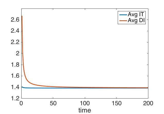
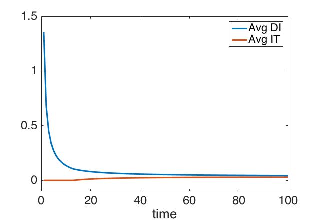
The average information transfer and average directed information, however, coincide as time goes to infinity. Intuitively, this can be explained as follows. Both average information transfer and average directed information can be written as a difference of two terms, where the first term is the same for both of them. The difference lies in the fact that, our definition of information transfer uses freezing, whereas, in directed information, one uses conditioning. However, as time goes to infinity, infinite step freezing and infinite step conditioning is the same and hence they converge to the same value.
Refer to caption
Figure 3: Comparison of average information transfer and average directed information for example (2).

For example, lets consider the example (2). In figure 3, we plot the average information transfer and average directed information from x1subscript𝑥1x_{1} to x30subscript𝑥30x_{30}. From the figure, we see that though average information transfer and average directed information differs in the initial stages, as the system evolves, they both converge to the same value.

3.2 Information transfer in linear dynamical system

The Eq. (5) provides formula for information transfer in general nonlinear system however for a special class of linear system analytical expression for the information transfer can be obtained. Consider the following linear time invariant dynamical system

z(t+1)=Az(t)+σξ(t)𝑧𝑡1𝐴𝑧𝑡𝜎𝜉𝑡\displaystyle z(t+1)=Az(t)+\sigma\xi(t) (11)

where z(t)N𝑧𝑡superscript𝑁z(t)\in\mathbb{R}^{N} and ξ(t)𝜉𝑡\xi(t) is vector valued Gaussian random variable with zero mean and unit variance. We assume that the initial conditions are Gaussian with covariance Σ(0)Σ0\Sigma(0). Since the system is linear, the distribution of the system state for all future time will remain Gaussian with covariance Σ(t)Σ𝑡\Sigma(t) satisfying

AΣ(t1)A+σ2I=Σ(t)𝐴Σ𝑡1superscript𝐴topsuperscript𝜎2𝐼Σ𝑡A\Sigma(t-1)A^{\top}+\sigma^{2}I=\Sigma(t)

To define the information transfer between various subspace we introduce following notation to split the A𝐴A matrix :

z(t+1)=(xy)=(AxAxyAyxAy)(xy)+σξ𝑧𝑡1matrixsuperscript𝑥superscript𝑦matrixsubscript𝐴𝑥subscript𝐴𝑥𝑦subscript𝐴𝑦𝑥subscript𝐴𝑦matrix𝑥𝑦𝜎𝜉\displaystyle z(t+1)=\begin{pmatrix}x^{{}^{\prime}}\\ y^{{}^{\prime}}\end{pmatrix}=\begin{pmatrix}A_{x}&A_{xy}\\ A_{yx}&A_{y}\end{pmatrix}\begin{pmatrix}x\\ y\end{pmatrix}+\sigma\xi (12)

The A𝐴A matrix can be further split using the subspace decomposition x=(x1,x2)𝑥superscriptsuperscriptsubscript𝑥1topsuperscriptsubscript𝑥2toptopx=(x_{1}^{\top},x_{2}^{\top})^{\top} as follows:

(AxAxyAyxAy)=(Ax1Ax1x2Ax1yAx2x1Ax2Ax2yAyx1Ayx2Ay)matrixsubscript𝐴𝑥subscript𝐴𝑥𝑦subscript𝐴𝑦𝑥subscript𝐴𝑦matrixsubscript𝐴subscript𝑥1subscript𝐴subscript𝑥1subscript𝑥2subscript𝐴subscript𝑥1𝑦subscript𝐴subscript𝑥2subscript𝑥1subscript𝐴subscript𝑥2subscript𝐴subscript𝑥2𝑦subscript𝐴𝑦subscript𝑥1subscript𝐴𝑦subscript𝑥2subscript𝐴𝑦\displaystyle\begin{pmatrix}A_{x}&A_{xy}\\ A_{yx}&A_{y}\end{pmatrix}=\begin{pmatrix}A_{x_{1}}&A_{x_{1}x_{2}}&A_{x_{1}y}\\ A_{x_{2}x_{1}}&A_{x_{2}}&A_{x_{2}y}\\ A_{yx_{1}}&A_{yx_{2}}&A_{y}\end{pmatrix} (13)

Based on the decomposition of the system A𝐴A matrix we can also decompose the covariance matrix ΣΣ\Sigma at time instant t𝑡t as follows.

Σ=(ΣxΣxyΣxyΣy)=(Σx1Σx1x2Σx1yΣx1x2Σx2Σx2yΣx1yΣx2yΣy)ΣmatrixsubscriptΣ𝑥subscriptΣ𝑥𝑦superscriptsubscriptΣ𝑥𝑦topsubscriptΣ𝑦matrixsubscriptΣsubscript𝑥1subscriptΣsubscript𝑥1subscript𝑥2subscriptΣsubscript𝑥1𝑦superscriptsubscriptΣsubscript𝑥1subscript𝑥2topsubscriptΣsubscript𝑥2subscriptΣsubscript𝑥2𝑦superscriptsubscriptΣsubscript𝑥1𝑦topsuperscriptsubscriptΣsubscript𝑥2𝑦topsubscriptΣ𝑦\displaystyle\Sigma=\begin{pmatrix}\Sigma_{x}&\Sigma_{xy}\\ \Sigma_{xy}^{\top}&\Sigma_{y}\end{pmatrix}=\begin{pmatrix}\Sigma_{x_{1}}&\Sigma_{x_{1}x_{2}}&\Sigma_{x_{1}y}\\ \Sigma_{x_{1}x_{2}}^{\top}&\Sigma_{x_{2}}&\Sigma_{x_{2}y}\\ \Sigma_{x_{1}y}^{\top}&\Sigma_{x_{2}y}^{\top}&\Sigma_{y}\end{pmatrix}
(14)

Using the above notation, we state following theorem providing explicit expression for information transfer in linear dynamical system during transient and steady state.

Theorem 7.

Consider the linear dynamical system (11) and associated splitting of state space in Eqs. (12) and (13). We have following expression for information transfer between various subspace

[Txy]tt+1=12log|AyxΣys(t)Ayx+σ2I|σ2superscriptsubscriptdelimited-[]subscript𝑇𝑥𝑦𝑡𝑡112subscript𝐴𝑦𝑥subscriptsuperscriptΣ𝑠𝑦𝑡superscriptsubscript𝐴𝑦𝑥topsuperscript𝜎2𝐼superscript𝜎2\displaystyle[T_{x\to y}]_{t}^{t+1}=\frac{1}{2}\log\frac{|A_{yx}\Sigma^{s}_{y}(t)A_{yx}^{\top}+\sigma^{2}I|}{\sigma^{2}} (15)

where Σys(t)=Σx(t)Σxy(t)Σy(t)1Σxy(t)subscriptsuperscriptΣ𝑠𝑦𝑡subscriptΣ𝑥𝑡subscriptΣ𝑥𝑦𝑡subscriptΣ𝑦superscript𝑡1subscriptΣ𝑥𝑦superscript𝑡top\Sigma^{s}_{y}(t)=\Sigma_{x}(t)-\Sigma_{xy}(t)\Sigma_{y}(t)^{-1}\Sigma_{xy}(t)^{\top} is the Schur complement of Σy(t)subscriptΣ𝑦𝑡\Sigma_{y}(t) in the matrix Σ(t)Σ𝑡\Sigma(t).

[Tx1y]tt+1=12log|AyxΣys(t)Ayx+σ2I||Ayx2(Σys)yx2(t)Ayx2+σ2I|superscriptsubscriptdelimited-[]subscript𝑇subscript𝑥1𝑦𝑡𝑡112subscript𝐴𝑦𝑥subscriptsuperscriptΣ𝑠𝑦𝑡superscriptsubscript𝐴𝑦𝑥topsuperscript𝜎2𝐼subscript𝐴𝑦subscript𝑥2subscriptsuperscriptsubscriptΣ𝑦𝑠𝑦subscript𝑥2𝑡superscriptsubscript𝐴𝑦subscript𝑥2topsuperscript𝜎2𝐼\displaystyle[T_{x_{1}\to y}]_{t}^{t+1}=\frac{1}{2}\log\frac{|A_{yx}\Sigma^{s}_{y}(t)A_{yx}^{\top}+\sigma^{2}I|}{|A_{yx_{2}}(\Sigma_{y}^{s})_{yx_{2}}(t)A_{yx_{2}}^{\top}+\sigma^{2}I|} (16)

where |||\cdot| is the determinant and (Σys)yx2subscriptsuperscriptsubscriptΣ𝑦𝑠𝑦subscript𝑥2(\Sigma_{y}^{s})_{yx_{2}} is the Schur complement of ΣysubscriptΣ𝑦\Sigma_{y} in the matrix

(Σx2Σx2yΣx2yΣy)matrixsubscriptΣsubscript𝑥2subscriptΣsubscript𝑥2𝑦superscriptsubscriptΣsubscript𝑥2𝑦topsubscriptΣ𝑦\begin{pmatrix}\Sigma_{x_{2}}&\Sigma_{x_{2}y}\\ \Sigma_{x_{2}y}^{\top}&\Sigma_{y}\end{pmatrix}
Proof.

From the formula of information transfer we have

[Txy]tt+1=H(ρ(y|y))H(ρ(y|y))superscriptsubscriptdelimited-[]subscript𝑇𝑥𝑦𝑡𝑡1𝐻𝜌conditionalsuperscript𝑦𝑦subscript𝐻italic-x̸𝜌conditionalsuperscript𝑦𝑦\displaystyle[T_{x\to y}]_{t}^{t+1}=H(\rho(y^{{}^{\prime}}|y))-H_{\not{x}}(\rho(y^{{}^{\prime}}|y))

So to compute the transfer, we need to know ρ(y|y)=ρ(y,y)ρ(y)𝜌conditionalsuperscript𝑦𝑦𝜌superscript𝑦𝑦𝜌𝑦\rho(y^{{}^{\prime}}|y)=\frac{\rho(y^{{}^{\prime}},y)}{\rho(y)} and ρ(y|y)subscript𝜌italic-x̸conditionalsuperscript𝑦𝑦\rho_{\not{x}}(y^{{}^{\prime}}|y). Furthermore, since all the probability density function involved are Gaussian, we use following formula for the entropy of Gaussian density function.

H(ρ(w))=12log((2πe)N|Σ(t)|)𝐻𝜌𝑤12superscript2𝜋𝑒𝑁Σ𝑡H(\rho(w))=\frac{1}{2}\log((2\pi e)^{N}|\Sigma(t)|)

for ρ(w)𝜌𝑤\rho(w) of the form

ρ(w)=1(2π)N2|Σ(t)|12exp(12wΣ(t)1z)𝜌𝑤1superscript2𝜋𝑁2superscriptΣ𝑡1212superscript𝑤topΣsuperscript𝑡1𝑧\rho(w)=\frac{1}{(2\pi)^{\frac{N}{2}}|\Sigma(t)|^{\frac{1}{2}}}\exp\left(-\frac{1}{2}w^{\top}\Sigma(t)^{-1}z\right)

Hence to compute the required transfer, we only need to know the covariance of ρ(y|y)𝜌conditionalsuperscript𝑦𝑦\rho(y^{{}^{\prime}}|y) and ρ(y|y)subscript𝜌italic-x̸conditionalsuperscript𝑦𝑦\rho_{\not{x}}(y^{{}^{\prime}}|y). The covariance matrix for the joint zsuperscript𝑧z^{{}^{\prime}} and z𝑧z is given by

Rzz=(ΣzΣzzΣzzΣz),Σz=(ΣxΣxyΣxyΣy)formulae-sequencesubscript𝑅superscript𝑧𝑧matrixsubscriptΣsuperscript𝑧subscriptΣsuperscript𝑧𝑧subscriptΣ𝑧superscript𝑧subscriptΣ𝑧subscriptΣ𝑧matrixsubscriptΣ𝑥subscriptΣ𝑥𝑦superscriptsubscriptΣ𝑥𝑦topsubscriptΣ𝑦R_{z^{{}^{\prime}}z}=\begin{pmatrix}\Sigma_{z^{{}^{\prime}}}&\Sigma_{z^{{}^{\prime}}z}\\ \Sigma_{zz^{{}^{\prime}}}&\Sigma_{z}\end{pmatrix},\;\;\Sigma_{z}=\begin{pmatrix}\Sigma_{x}&\Sigma_{xy}\\ \Sigma_{xy}^{\top}&\Sigma_{y}\end{pmatrix}

where Σz=AΣzA+σ2IsubscriptΣsuperscript𝑧𝐴subscriptΣ𝑧superscript𝐴topsuperscript𝜎2𝐼\Sigma_{z^{{}^{\prime}}}=A\Sigma_{z}A^{\top}+\sigma^{2}I, Σzz=ΣzAsubscriptΣ𝑧superscript𝑧subscriptΣ𝑧superscript𝐴top\Sigma_{zz^{{}^{\prime}}}=\Sigma_{z}A^{\top}, Σzz=AΣz=ΣzzsubscriptΣsuperscript𝑧𝑧𝐴subscriptΣ𝑧superscriptsubscriptΣ𝑧superscript𝑧top\Sigma_{z^{{}^{\prime}}z}=A\Sigma_{z}=\Sigma_{zz^{{}^{\prime}}}^{\top} Hence, we have

Ryy=(ΣyΣyyΣyyΣy),y|y𝒩(,ΣyΣyyΣy1Σyy)formulae-sequencesubscript𝑅superscript𝑦𝑦matrixsubscriptΣsuperscript𝑦subscriptΣsuperscript𝑦𝑦superscriptsubscriptΣsuperscript𝑦𝑦topsubscriptΣ𝑦similar-toconditionalsuperscript𝑦𝑦𝒩subscriptΣsuperscript𝑦subscriptΣsuperscript𝑦𝑦superscriptsubscriptΣ𝑦1superscriptsubscriptΣsuperscript𝑦𝑦topR_{y^{{}^{\prime}}y}=\begin{pmatrix}\Sigma_{y^{{}^{\prime}}}&\Sigma_{y^{{}^{\prime}}y}\\ \Sigma_{y^{{}^{\prime}}y}^{\top}&\Sigma_{y}\end{pmatrix},y^{{}^{\prime}}|y\sim{\cal N}(-,\Sigma_{y^{{}^{\prime}}}-\Sigma_{y^{{}^{\prime}}y}\Sigma_{y}^{-1}\Sigma_{y^{{}^{\prime}}y}^{\top})
Σy=AyxΣxAyx+AyΣxyAyx+AyxΣxyAysubscriptΣsuperscript𝑦subscript𝐴𝑦𝑥subscriptΣ𝑥superscriptsubscript𝐴𝑦𝑥topsubscript𝐴𝑦subscriptΣ𝑥𝑦superscriptsubscript𝐴𝑦𝑥topsubscript𝐴𝑦𝑥subscriptΣ𝑥𝑦superscriptsubscript𝐴𝑦top\displaystyle\Sigma_{y^{{}^{\prime}}}=A_{yx}\Sigma_{x}A_{yx}^{\top}+A_{y}\Sigma_{xy}A_{yx}^{\top}+A_{yx}\Sigma_{xy}A_{y}^{\top}
+AyΣyAy+σ2Isubscript𝐴𝑦subscriptΣ𝑦superscriptsubscript𝐴𝑦topsuperscript𝜎2𝐼\displaystyle+A_{y}\Sigma_{y}A_{y}^{\top}+\sigma^{2}I
Σyy=AyxΣxy+AyΣysubscriptΣsuperscript𝑦𝑦subscript𝐴𝑦𝑥subscriptΣ𝑥𝑦subscript𝐴𝑦subscriptΣ𝑦\Sigma_{y^{{}^{\prime}}y}=A_{yx}\Sigma_{xy}+A_{y}\Sigma_{y}

Note that since the entropy is function of covariance, we ignore the explicit computation of mean for the underlying Gaussian random variable. After simplification, we obtain

ρ(y|y)𝒩(,Ayx(ΣxΣxyΣy1Σxy)Ayx+σ2I).similar-to𝜌conditionalsuperscript𝑦𝑦𝒩subscript𝐴𝑦𝑥subscriptΣ𝑥subscriptΣ𝑥𝑦superscriptsubscriptΣ𝑦1superscriptsubscriptΣ𝑥𝑦topsuperscriptsubscript𝐴𝑦𝑥topsuperscript𝜎2𝐼\rho(y^{{}^{\prime}}|y)\sim{\cal N}(-,A_{yx}(\Sigma_{x}-\Sigma_{xy}\Sigma_{y}^{-1}\Sigma_{xy}^{\top})A_{yx}^{\top}+\sigma^{2}I).

For ρ(y|y)subscript𝜌italic-x̸conditionalsuperscript𝑦𝑦\rho_{\not{x}}(y^{{}^{\prime}}|y) we look at the system, y=Ayy+σξysuperscript𝑦subscript𝐴𝑦𝑦𝜎subscript𝜉𝑦y^{{}^{\prime}}=A_{y}y+\sigma\xi_{y}. Hence, we have ρ(y|y)𝒩(,σ2I)similar-tosubscript𝜌italic-x̸conditionalsuperscript𝑦𝑦𝒩superscript𝜎2𝐼\rho_{\not{x}}(y^{{}^{\prime}}|y)\sim{\cal N}\left(-,{\sigma^{2}}I\right). Hence we have

Txy(t)=12log|AyxΣys(t)Ayx+σ2I|σ2subscript𝑇𝑥𝑦𝑡12subscript𝐴𝑦𝑥subscriptsuperscriptΣ𝑠𝑦𝑡superscriptsubscript𝐴𝑦𝑥topsuperscript𝜎2𝐼superscript𝜎2T_{x\to y}(t)=\frac{1}{2}\log\frac{|A_{yx}\Sigma^{s}_{y}(t)A_{yx}^{\top}+\sigma^{2}I|}{\sigma^{2}}

where Σys(t)=Σx(t)Σxy(t)Σy(t)1Σxy(t)subscriptsuperscriptΣ𝑠𝑦𝑡subscriptΣ𝑥𝑡subscriptΣ𝑥𝑦𝑡subscriptΣ𝑦superscript𝑡1subscriptΣ𝑥𝑦superscript𝑡top\Sigma^{s}_{y}(t)=\Sigma_{x}(t)-\Sigma_{xy}(t)\Sigma_{y}(t)^{-1}\Sigma_{xy}(t)^{\top}.

To compute the information transfer from x1ysubscript𝑥1𝑦x_{1}\to y, we need to compute covariance for ρ1(y|y)subscript𝜌subscriptitalic-x̸1conditionalsuperscript𝑦𝑦\rho_{\not{x}_{1}}(y^{{}^{\prime}}|y). Hence, we look at the system where x1subscript𝑥1x_{1} is absent. Hence, we look at

x2=Ax2x2+Ax2yy+ξx2superscriptsubscript𝑥2subscript𝐴subscript𝑥2subscript𝑥2subscript𝐴subscript𝑥2𝑦𝑦subscript𝜉subscript𝑥2\displaystyle x_{2}^{{}^{\prime}}=A_{x_{2}}x_{2}+A_{x_{2}y}y+\xi_{x_{2}}
y=Ayx2x2+Ayy+ξysuperscript𝑦subscript𝐴𝑦subscript𝑥2subscript𝑥2subscript𝐴𝑦𝑦subscript𝜉𝑦\displaystyle y^{{}^{\prime}}=A_{yx_{2}}x_{2}+A_{y}y+\xi_{y} (17)

The expression for ρ(y|y)𝜌conditionalsuperscript𝑦𝑦\rho(y^{{}^{\prime}}|y) remains unchanged from the previous case. To compute ρ1(y|y)subscript𝜌subscriptitalic-x̸1conditionalsuperscript𝑦𝑦\rho_{\not x_{1}}(y^{{}^{\prime}}|y), we use system equation (17) and use procedure similar to one used in the derivation of ρ(y|y)subscript𝜌italic-x̸conditionalsuperscript𝑦𝑦\rho_{\not x}(y^{{}^{\prime}}|y) with x𝑥x replaced with x1subscript𝑥1x_{1}. Hence, we have

ρ1(y|y)=𝒩(,Ayx2(Σys)yx2(t)Ayx2+σ2I)subscript𝜌subscriptitalic-x̸1conditionalsuperscript𝑦𝑦𝒩subscript𝐴𝑦subscript𝑥2subscriptsuperscriptsubscriptΣ𝑦𝑠𝑦subscript𝑥2𝑡superscriptsubscript𝐴𝑦subscript𝑥2topsuperscript𝜎2𝐼\displaystyle\rho_{\not{x_{1}}}(y^{{}^{\prime}}|y)=\mathcal{N}\left(-,A_{yx_{2}}(\Sigma_{y}^{s})_{yx_{2}}(t)A_{yx_{2}}^{\top}+\sigma^{2}I\right) (18)

where,

(Σys)yx2(t)=(Σx2(t)Σx2y(t)Σy1(t)Σx2y(t)).subscriptsuperscriptsubscriptΣ𝑦𝑠𝑦subscript𝑥2𝑡subscriptΣsubscript𝑥2𝑡subscriptΣsubscript𝑥2𝑦𝑡superscriptsubscriptΣ𝑦1𝑡superscriptsubscriptΣsubscript𝑥2𝑦top𝑡\displaystyle(\Sigma_{y}^{s})_{yx_{2}}(t)=(\Sigma_{x_{2}}(t)-\Sigma_{x_{2}y}(t)\Sigma_{y}^{-1}(t)\Sigma_{x_{2}y}^{\top}(t)).

Hence,

[Tx1y]tt+1=12log|AyxΣys(t)Ayx+σ2I||Ayx2(Σys)yx2(t)Ayx2+σ2I|superscriptsubscriptdelimited-[]subscript𝑇subscript𝑥1𝑦𝑡𝑡112subscript𝐴𝑦𝑥subscriptsuperscriptΣ𝑠𝑦𝑡superscriptsubscript𝐴𝑦𝑥topsuperscript𝜎2𝐼subscript𝐴𝑦subscript𝑥2subscriptsuperscriptsubscriptΣ𝑦𝑠𝑦subscript𝑥2𝑡superscriptsubscript𝐴𝑦subscript𝑥2topsuperscript𝜎2𝐼\displaystyle[T_{x_{1}\to y}]_{t}^{t+1}=\frac{1}{2}\log\frac{|A_{yx}\Sigma^{s}_{y}(t)A_{yx}^{\top}+\sigma^{2}I|}{|A_{yx_{2}}(\Sigma_{y}^{s})_{yx_{2}}(t)A_{yx_{2}}^{\top}+\sigma^{2}I|} (19)

. ∎

The results from the above theorem can be used to provide general expression for information transfer between scalar state zisubscript𝑧𝑖z_{i} and zjsubscript𝑧𝑗z_{j} for linear network system. In particular with no loss of generality we can assume zi=z1subscript𝑧𝑖subscript𝑧1z_{i}=z_{1} and zj=z2subscript𝑧𝑗subscript𝑧2z_{j}=z_{2}, then the expression for Tz1z2subscript𝑇subscript𝑧1subscript𝑧2T_{z_{1}\to z_{2}} can be obtained from (16) by defining

x1:=z1,y=z2,x2:=(z3,,zN)formulae-sequenceassignsubscript𝑥1subscript𝑧1formulae-sequence𝑦subscript𝑧2assignsubscript𝑥2subscript𝑧3subscript𝑧𝑁x_{1}:=z_{1},\;\;\;y=z_{2},\;\;x_{2}:=(z_{3},\ldots,z_{N})

The formula for n𝑛n-step transfer can also be derived in a similar manner, where one has to look at the n𝑛n-step covariance matrix.

For linear systems with Gaussian noise, the one step zero transfer can be characterized by looking at system matrix A𝐴A. In particular, we have the following theorem.

Theorem 8.

Azjzi=0subscript𝐴subscript𝑧𝑗subscript𝑧𝑖0A_{z_{j}z_{i}}=0, iff [Tzizj]tt+1=0superscriptsubscriptdelimited-[]subscript𝑇subscript𝑧𝑖subscript𝑧𝑗𝑡𝑡10[T_{z_{i}\to z_{j}}]_{t}^{t+1}=0.

Proof.

The proof follows from formula (16).

3.3 Information transfer and Causal Inference in Nonlinear Systems

In this subsection we connect information transfer and causal inference for general nolinear systems. However, we will consider systems without noise. In particular, we consider the system

zt+1=T(zt)subscript𝑧𝑡1𝑇subscript𝑧𝑡\displaystyle z_{t+1}=T(z_{t}) (20)

where T:nn:𝑇superscript𝑛superscript𝑛T:\mathbb{R}^{n}\to\mathbb{R}^{n} is assumed to be at least continuous and z(t)n𝑧𝑡superscript𝑛z(t)\in\mathbb{R}^{n}. In component form, equation (20) can be written as

zt+11=T1(zt1,zt2,,ztn)zt+12=T2(zt1,zt2,,ztn)zt+1n=Tn(zt1,zt2,,ztn)superscriptsubscript𝑧𝑡11absentsubscript𝑇1superscriptsubscript𝑧𝑡1superscriptsubscript𝑧𝑡2superscriptsubscript𝑧𝑡𝑛superscriptsubscript𝑧𝑡12absentsubscript𝑇2superscriptsubscript𝑧𝑡1superscriptsubscript𝑧𝑡2superscriptsubscript𝑧𝑡𝑛missing-subexpressionsuperscriptsubscript𝑧𝑡1𝑛absentsubscript𝑇𝑛superscriptsubscript𝑧𝑡1superscriptsubscript𝑧𝑡2superscriptsubscript𝑧𝑡𝑛\displaystyle\begin{aligned} z_{t+1}^{1}&=T_{1}(z_{t}^{1},z_{t}^{2},\cdots,z_{t}^{n})\\ z_{t+1}^{2}&=T_{2}(z_{t}^{1},z_{t}^{2},\cdots,z_{t}^{n})\\ &\vdots\\ z_{t+1}^{n}&=T_{n}(z_{t}^{1},z_{t}^{2},\cdots,z_{t}^{n})\\ \end{aligned} (21)

Information transfer between the states of a dynamical system is defined in terms of difference of certain entropies, as the dynamical system evolves in time. As such to compute the information transfer, it is necessary to know the evolution of densities. This is given by the Perron-Frobenius (PF) operator

:1(n)1(n):superscript1superscript𝑛superscript1superscript𝑛\displaystyle\mathbb{P}:\mathcal{L}^{1}(\mathbb{R}^{n})\to\mathcal{L}^{1}(\mathbb{R}^{n}) (22)

and is defined as

ωρ(z)𝑑z=T1(ω)ρ(z)𝑑zsubscript𝜔𝜌𝑧differential-d𝑧subscriptsuperscript𝑇1𝜔𝜌𝑧differential-d𝑧\displaystyle\int_{\omega}\mathbb{P}\rho(z)dz=\int_{T^{-1}(\omega)}\rho(z)dz (23)

for any ω(n)𝜔superscript𝑛\omega\in\mathcal{B}(\mathbb{R}^{n}), where (n)superscript𝑛\mathcal{B}(\mathbb{R}^{n}) is the Borel σ𝜎\sigma-algebra on nsuperscript𝑛\mathbb{R}^{n}. When T𝑇T is non-singular and invertible, the PF operator can be written explicitly as

ρ(z)=ρ[T1(z)]|J1|𝜌𝑧𝜌delimited-[]superscript𝑇1𝑧superscript𝐽1\displaystyle\mathbb{P}\rho(z)=\rho[T^{-1}(z)]|J^{-1}| (24)

where J𝐽J is the Jacobian of T𝑇T and |||\cdot| signify the determinant. The joint density ρ(z)𝜌𝑧\rho(z) is used to define the Shannon entropy

H(z)=Ωρ(z)logρ(z)𝑑z𝐻𝑧subscriptΩ𝜌𝑧𝜌𝑧differential-d𝑧\displaystyle H(z)=-\int_{\Omega}\rho(z)\log\rho(z)dz (25)

where ΩΩ\Omega is the sample space.

Assumption 9.

We assume ΩΩ\Omega to be Cartesian product of Ω1,Ω2,,ΩnsubscriptΩ1subscriptΩ2subscriptΩ𝑛\Omega_{1},\Omega_{2},\cdots,\Omega_{n}, in which z1,z2,,znsuperscript𝑧1superscript𝑧2superscript𝑧𝑛z^{1},z^{2},\cdots,z^{n} are respectively lying. Here each ΩisubscriptΩ𝑖\Omega_{i} are open in \mathbb{R}, for i=1,2,,n𝑖12𝑛i=1,2,\cdots,n.

The marginal entropy of any variable of interest, say z1subscript𝑧1z_{1} is defined as

H(z1)=Ω1ρ1(z1)logρ1(z1)𝑑z1𝐻superscript𝑧1subscriptsubscriptΩ1subscript𝜌1superscript𝑧1subscript𝜌1superscript𝑧1differential-dsuperscript𝑧1\displaystyle H(z^{1})=-\int_{\Omega_{1}}\rho_{1}(z^{1})\log\rho_{1}(z^{1})dz^{1} (26)

where ρ1=ρ(z1)=Ω2nρ(z)𝑑z2𝑑z3𝑑znsubscript𝜌1𝜌superscript𝑧1subscriptsubscriptΩ2𝑛𝜌𝑧differential-dsuperscript𝑧2differential-dsuperscript𝑧3differential-dsuperscript𝑧𝑛\rho_{1}=\rho(z^{1})=\int_{\Omega_{2n}}\rho(z)dz^{2}dz^{3}\cdots dz^{n} is the marginal distribution of z1superscript𝑧1z^{1}. Here we use the notation

Ωjn=Ωj×Ωj+1××Ωn,1jn, and Ω1n=Ω.formulae-sequenceformulae-sequencesubscriptΩ𝑗𝑛subscriptΩ𝑗subscriptΩ𝑗1subscriptΩ𝑛1𝑗𝑛 and subscriptΩ1𝑛Ω\displaystyle\Omega_{jn}=\Omega_{j}\times\Omega_{j+1}\times\cdots\times\Omega_{n},\quad 1\leq j\leq n,\textnormal{ and }\Omega_{1n}=\Omega. (27)

We further use the notation

ρ=ρ(z1,zi1,zi+1,,zn)subscript𝜌italic-i̸𝜌superscript𝑧1superscript𝑧𝑖1superscript𝑧𝑖1superscript𝑧𝑛\displaystyle\rho_{\not{i}}=\rho(z^{1},\cdots z^{i-1},z^{i+1},\cdots,z^{n})
=Ωiρ(z1,zi1,zi+1,,zn)𝑑ziabsentsubscriptsubscriptΩ𝑖𝜌superscript𝑧1superscript𝑧𝑖1superscript𝑧𝑖1superscript𝑧𝑛differential-dsuperscript𝑧𝑖\displaystyle=\int_{\Omega_{i}}\rho(z^{1},\cdots z^{i-1},z^{i+1},\cdots,z^{n})dz^{i}
ρ=ρ(z1,zi1,zi+1,,zj1,zj+1,zn)subscript𝜌italic-i̸italic-j̸𝜌superscript𝑧1superscript𝑧𝑖1superscript𝑧𝑖1superscript𝑧𝑗1superscript𝑧𝑗1superscript𝑧𝑛\displaystyle\rho_{\not{i}\not{j}}=\rho(z^{1},\cdots z^{i-1},z^{i+1},\cdots,z^{j-1},z^{j+1}\cdots,z^{n})
=Ωi×Ωjρ(z1,zi1,zi+1,,zj1,zj+1,,zn)𝑑zi𝑑zjabsentsubscriptsubscriptΩ𝑖subscriptΩ𝑗𝜌superscript𝑧1superscript𝑧𝑖1superscript𝑧𝑖1superscript𝑧𝑗1superscript𝑧𝑗1superscript𝑧𝑛differential-dsuperscript𝑧𝑖differential-dsuperscript𝑧𝑗\displaystyle=\int_{\Omega_{i}\times\Omega_{j}}\rho(z^{1},\cdots z^{i-1},z^{i+1},\cdots,z^{j-1},z^{j+1},\cdots,z^{n})dz^{i}dz^{j}

With this, we state the following theorem which connects information transfer with causal inference.

Theorem 10.

If Tjsubscript𝑇𝑗T_{j} is independent of zisuperscript𝑧𝑖z^{i}, then Tzizj=0subscript𝑇superscript𝑧𝑖superscript𝑧𝑗0T_{z^{i}\to z^{j}}=0. At the same time, Tzizjsubscript𝑇superscript𝑧𝑖superscript𝑧𝑗T_{z^{i}\to z^{j}} need not be zero if Tjsubscript𝑇𝑗T_{j} does not rely on zisuperscript𝑧𝑖z^{i}.

Proof.

Without loss of generality, we assume i=2𝑖2i=2 and j=1𝑗1j=1, so that we look at the information transfer from z2superscript𝑧2z^{2} to z1superscript𝑧1z^{1}. We consider the system zt+1=T(zt)subscript𝑧𝑡1𝑇subscript𝑧𝑡z_{t+1}=T(z_{t}) given in component form as in (21). Define z^ti=zt+1isuperscriptsubscript^𝑧𝑡𝑖superscriptsubscript𝑧𝑡1𝑖\hat{z}_{t}^{i}=z_{t+1}^{i} and consider the dynamical system

zt+1i=Ti(z)z^t+1i=Ti(z^)superscriptsubscript𝑧𝑡1𝑖subscript𝑇𝑖𝑧superscriptsubscript^𝑧𝑡1𝑖subscript𝑇𝑖^𝑧\displaystyle\begin{aligned} z_{t+1}^{i}&=&T_{i}(z)\\ \hat{z}_{t+1}^{i}&=&T_{i}(\hat{z})\end{aligned} (28)

for i=1,2,,n𝑖12𝑛i=1,2,\cdots,n. Now, from (LABEL:info_trnasfer_eqv),

Tz2z1subscript𝑇superscript𝑧2superscript𝑧1\displaystyle T_{z^{2}\to z^{1}} =\displaystyle= H(zt+11,zt1)H2(zt+11,zt1)𝐻superscriptsubscript𝑧𝑡11superscriptsubscript𝑧𝑡1subscript𝐻subscriptitalic-z̸2superscriptsubscript𝑧𝑡11superscriptsubscript𝑧𝑡1\displaystyle H(z_{t+1}^{1},z_{t}^{1})-H_{\not{z}_{2}}(z_{t+1}^{1},z_{t}^{1}) (29)
=\displaystyle= H(zt+11,z^t+11)H2(zt+11,z^t+11)𝐻superscriptsubscript𝑧𝑡11superscriptsubscript^𝑧𝑡11subscript𝐻subscriptitalic-z̸2superscriptsubscript𝑧𝑡11superscriptsubscript^𝑧𝑡11\displaystyle H(z_{t+1}^{1},\hat{z}_{t+1}^{1})-H_{\not{z}_{2}}(z_{t+1}^{1},\hat{z}_{t+1}^{1})

It is given that T1(z)subscript𝑇1𝑧T_{1}(z) is independent of z2superscript𝑧2z^{2}. Hence, T1(z^)subscript𝑇1^𝑧T_{1}(\hat{z}) is independent of z^2superscript^𝑧2\hat{z}^{2} and also z2superscript𝑧2z^{2}. To prove that if T1(z)subscript𝑇1𝑧T_{1}(z) is independent of z2subscript𝑧2z_{2}, then Tz2z1=0subscript𝑇subscript𝑧2subscript𝑧10T_{z_{2}\to z_{1}}=0, we have to show

H(zt+11,z^t+11)=H2(zt+11,z^t+11)𝐻superscriptsubscript𝑧𝑡11superscriptsubscript^𝑧𝑡11subscript𝐻subscriptitalic-z̸2superscriptsubscript𝑧𝑡11superscriptsubscript^𝑧𝑡11\displaystyle H(z_{t+1}^{1},\hat{z}_{t+1}^{1})=H_{\not{z}_{2}}(z_{t+1}^{1},\hat{z}_{t+1}^{1})

Let U𝑈U be the sample space where the system (28) evolves. Note that U𝑈U satisfies assumption (9) and we use the notation defined in (27). For notational convenience we use the notation xt1superscriptsubscript𝑥𝑡1x_{t}^{1} to signify the subspace (zt1,z^t1)superscriptsuperscriptsubscript𝑧𝑡1superscriptsubscript^𝑧𝑡1top(z_{t}^{1},\hat{z}_{t}^{1})^{\top}, xt2=zt2superscriptsubscript𝑥𝑡2superscriptsubscript𝑧𝑡2x_{t}^{2}=z_{t}^{2}, yt=z^t2subscript𝑦𝑡superscriptsubscript^𝑧𝑡2y_{t}=\hat{z}_{t}^{2}, xti=(zti,z^ti)superscriptsubscript𝑥𝑡𝑖superscriptsuperscriptsubscript𝑧𝑡𝑖superscriptsubscript^𝑧𝑡𝑖topx_{t}^{i}=(z_{t}^{i},\hat{z}_{t}^{i})^{\top} for i=3,,n𝑖3𝑛i=3,\cdots,n. Similarly we define Uisubscript𝑈𝑖U_{i} and Uysubscript𝑈𝑦U_{y}. Hence we need to prove

H(xt+11)=H2(xt+11)𝐻superscriptsubscript𝑥𝑡11subscript𝐻subscriptitalic-x̸2superscriptsubscript𝑥𝑡11\displaystyle H(x_{t+1}^{1})=H_{\not{x}_{2}}(x_{t+1}^{1})

The dynamical system (28) can be written as

xt+1i=ϕi(xt,yt)xt+12=ϕ2(xt,yt)yt+1=ϕy(xt,yt)missing-subexpressionsuperscriptsubscript𝑥𝑡1𝑖subscriptitalic-ϕ𝑖subscript𝑥𝑡subscript𝑦𝑡missing-subexpressionsuperscriptsubscript𝑥𝑡12subscriptitalic-ϕ2subscript𝑥𝑡subscript𝑦𝑡missing-subexpressionsubscript𝑦𝑡1subscriptitalic-ϕ𝑦subscript𝑥𝑡subscript𝑦𝑡\displaystyle\begin{aligned} &x_{t+1}^{i}=\phi_{i}(x_{t},y_{t})\\ &x_{t+1}^{2}=\phi_{2}(x_{t},y_{t})\\ &y_{t+1}=\phi_{y}(x_{t},y_{t})\end{aligned} (30)

for i=1,3,,n𝑖13𝑛i=1,3,\cdots,n and ϕi=(Ti,Ti)subscriptitalic-ϕ𝑖superscriptsubscript𝑇𝑖subscript𝑇𝑖top\phi_{i}=(T_{i},T_{i})^{\top}, ϕ2=T2subscriptitalic-ϕ2subscript𝑇2\phi_{2}=T_{2} and ϕy=T2subscriptitalic-ϕ𝑦subscript𝑇2\phi_{y}=T_{2}. Define Φ=(ϕiϕ2ϕy)Φsuperscriptmatrixsuperscriptsubscriptitalic-ϕ𝑖topsubscriptitalic-ϕ2subscriptitalic-ϕ𝑦top\Phi=\begin{pmatrix}\phi_{i}^{\top}&\phi_{2}&\phi_{y}\end{pmatrix}^{\top}. For any subset of U~1subscript~𝑈1\tilde{U}_{1}, u~1U~1subscript~𝑢1subscript~𝑈1\tilde{u}_{1}\in\tilde{U}_{1}, we have

u~1(ρ2)1(x1)𝑑x1subscriptsubscript~𝑢1subscriptsubscript𝜌superscriptitalic-x̸21superscript𝑥1differential-dsuperscript𝑥1\displaystyle\int_{\tilde{u}_{1}}(\mathbb{P}\rho_{\not{x}^{2}})_{1}(x^{1})dx^{1} =\displaystyle= u~1×U3n×Uy(ρ2)(x1,y,x3,,xn)subscriptsubscript~𝑢1subscript𝑈3𝑛subscript𝑈𝑦subscript𝜌subscriptitalic-x̸2superscript𝑥1𝑦superscript𝑥3superscript𝑥𝑛\displaystyle\int_{\tilde{u}_{1}\times U_{3n}\times U_{y}}(\mathbb{P}\rho_{\not{x}_{2}})(x^{1},y,x^{3},\cdots,x^{n})
×dx1dx3dxndyabsent𝑑superscript𝑥1𝑑superscript𝑥3𝑑superscript𝑥𝑛𝑑𝑦\displaystyle\times dx^{1}dx^{3}\cdots dx^{n}dy
=\displaystyle= Φ1(u~1×U3n×Uy)ρ2(x1,y,x3,,xn)subscriptsuperscriptsubscriptΦnot-21subscript~𝑢1subscript𝑈3𝑛subscript𝑈𝑦subscript𝜌subscriptitalic-x̸2superscript𝑥1𝑦superscript𝑥3superscript𝑥𝑛\displaystyle\int_{\Phi_{\not{2}}^{-1}(\tilde{u}_{1}\times U_{3n}\times U_{y})}\rho_{\not{x}_{2}}(x^{1},y,x^{3},\cdots,x^{n})
×dx1dx3dxndyabsent𝑑superscript𝑥1𝑑superscript𝑥3𝑑superscript𝑥𝑛𝑑𝑦\displaystyle\times dx^{1}dx^{3}\cdots dx^{n}dy

Now111In the proof, Φ11u~1superscriptsubscriptΦ1not-21subscript~𝑢1\Phi_{1\not{2}}^{-1}\tilde{u}_{1} and ϕ11u~1superscriptsubscriptitalic-ϕ11subscript~𝑢1\phi_{1}^{-1}\tilde{u}_{1} is the projection of the Cartesian product on the subspace x1superscript𝑥1x^{1}.,

Φ1(u~1×U3n×Uy)=Φ11u~1×U3n×UysuperscriptsubscriptΦnot-21subscript~𝑢1subscript𝑈3𝑛subscript𝑈𝑦superscriptsubscriptΦ1not-21subscript~𝑢1subscript𝑈3𝑛subscript𝑈𝑦\displaystyle{\Phi_{\not{2}}^{-1}(\tilde{u}_{1}\times U_{3n}\times U_{y})}=\Phi_{1\not{2}}^{-1}\tilde{u}_{1}\times U_{3n}\times U_{y} (31)

Hence,

u~1(ρ2)1(x1)𝑑x1subscriptsubscript~𝑢1subscriptsubscript𝜌superscriptitalic-x̸21superscript𝑥1differential-dsuperscript𝑥1\displaystyle\int_{\tilde{u}_{1}}(\mathbb{P}\rho_{\not{x}^{2}})_{1}(x^{1})dx^{1} =\displaystyle= Φ11u~1𝑑x1subscriptsuperscriptsubscriptΦ1not-21subscript~𝑢1differential-dsuperscript𝑥1\displaystyle\int_{\Phi_{1\not{2}}^{-1}\tilde{u}_{1}}dx^{1}
U3n×Uyρ2(x1,x3,,xn,y)\displaystyle\quad\cdot\int_{U_{3n}\times U_{y}}\rho_{\not{x}^{2}}(x^{1},x^{3},\cdots,x^{n},y)
×dx1dx3dxndyabsent𝑑superscript𝑥1𝑑superscript𝑥3𝑑superscript𝑥𝑛𝑑𝑦\displaystyle\quad\times dx^{1}dx^{3}\cdots dx^{n}dy
=\displaystyle= Φ11u~1ρ1(x1)𝑑x1subscriptsuperscriptsubscriptΦ1not-21subscript~𝑢1subscript𝜌1superscript𝑥1differential-dsuperscript𝑥1\displaystyle\int_{\Phi_{1\not{2}}^{-1}\tilde{u}_{1}}\rho_{1}(x^{1})dx^{1}
=\displaystyle= ϕ11u~1ρ1(x1)𝑑x1subscriptsuperscriptsubscriptitalic-ϕ11subscript~𝑢1subscript𝜌1superscript𝑥1differential-dsuperscript𝑥1\displaystyle\int_{{\phi_{1}}^{-1}\tilde{u}_{1}}\rho_{1}(x^{1})dx^{1}

where the last equality follows from the fact that ϕ1subscriptitalic-ϕ1\phi_{1} and hence ϕ11superscriptsubscriptitalic-ϕ11\phi_{1}^{-1} is independent of x2subscript𝑥2x_{2}.

Again,

u~1(ρ)1(x1)𝑑x1subscriptsubscript~𝑢1subscript𝜌1superscript𝑥1differential-dsuperscript𝑥1\displaystyle\int_{\tilde{u}_{1}}(\mathbb{P}\rho)_{1}(x^{1})dx^{1} =\displaystyle= u~1×U2n×Uyρ(x,y)𝑑x𝑑ysubscriptsubscript~𝑢1subscript𝑈2𝑛subscript𝑈𝑦𝜌𝑥𝑦differential-d𝑥differential-d𝑦\displaystyle\int_{\tilde{u}_{1}\times U_{2}n\times U_{y}}\mathbb{P}\rho(x,y)dxdy
=\displaystyle= Φ1(u~1×U2n×Uy)ρ(x,y)𝑑x𝑑ysubscriptsuperscriptΦ1subscript~𝑢1subscript𝑈2𝑛subscript𝑈𝑦𝜌𝑥𝑦differential-d𝑥differential-d𝑦\displaystyle\int_{\Phi^{-1}({\tilde{u}_{1}\times U_{2n}\times U_{y}})}\rho(x,y)dxdy
=\displaystyle= ϕ1u~1×U2n×Uyρ(x,y)𝑑x𝑑ysubscriptsuperscriptitalic-ϕ1subscript~𝑢1subscript𝑈2𝑛subscript𝑈𝑦𝜌𝑥𝑦differential-d𝑥differential-d𝑦\displaystyle\int_{\phi^{-1}\tilde{u}_{1}\times U_{2n}\times U_{y}}\rho(x,y)dxdy
=\displaystyle= ϕ11u~1𝑑x1U2n×Uyρ(x)𝑑x2𝑑xn𝑑ysubscriptsuperscriptsubscriptitalic-ϕ11subscript~𝑢1differential-dsuperscript𝑥1subscriptsubscript𝑈2𝑛subscript𝑈𝑦𝜌𝑥differential-dsuperscript𝑥2differential-dsuperscript𝑥𝑛differential-d𝑦\displaystyle\int_{\phi_{1}^{-1}\tilde{u}_{1}}dx^{1}\int_{U_{2n}\times U_{y}}\rho(x)dx^{2}\cdots dx^{n}dy
=\displaystyle= ϕ11u~1ρ1(x1)𝑑x1.subscriptsuperscriptsubscriptitalic-ϕ11subscript~𝑢1subscript𝜌1superscript𝑥1differential-dsuperscript𝑥1\displaystyle\int_{\phi_{1}^{-1}\tilde{u}_{1}}\rho_{1}(x^{1})dx^{1}.

Hence,

u~1(ρ2)1(x1)𝑑x1=u~1(ρ)1(x1)𝑑x1subscriptsubscript~𝑢1subscriptsubscript𝜌superscriptitalic-x̸21superscript𝑥1differential-dsuperscript𝑥1subscriptsubscript~𝑢1subscript𝜌1superscript𝑥1differential-dsuperscript𝑥1\displaystyle\int_{\tilde{u}_{1}}(\mathbb{P}\rho_{\not{x}^{2}})_{1}(x^{1})dx^{1}=\int_{\tilde{u}_{1}}(\mathbb{P}\rho)_{1}(x^{1})dx^{1} (32)

for any u~1U1subscript~𝑢1subscript𝑈1\tilde{u}_{1}\in U_{1}. Hence, (ρ2)1=(ρ)1subscriptsubscript𝜌superscriptitalic-x̸21subscript𝜌1(\mathbb{P}\rho_{\not{x}^{2}})_{1}=(\mathbb{P}\rho)_{1} almost everywhere, when ϕ1subscriptitalic-ϕ1\phi_{1} is independent of x2superscript𝑥2x^{2}. Now, in [liang_discrete] it was shown that

H2(xt+11)subscript𝐻superscriptitalic-x̸2superscriptsubscript𝑥𝑡11\displaystyle H_{\not{x}^{2}}(x_{t+1}^{1}) =\displaystyle= U(ρ2)1(y1)log((ρ2)1(y1))subscript𝑈subscriptsubscript𝜌superscriptitalic-x̸21superscript𝑦1subscriptsubscript𝜌superscriptitalic-x̸21superscript𝑦1\displaystyle-\int_{U}(\mathbb{P}\rho_{\not{x}^{2}})_{1}(y^{1})\log((\mathbb{P}\rho_{\not{x}^{2}})_{1}(y^{1}))
ρ(x2|x1,x3,xn,y)absent𝜌conditionalsuperscript𝑥2superscript𝑥1superscript𝑥3superscript𝑥𝑛𝑦\displaystyle\cdot\rho(x^{2}|x^{1},x^{3}\cdots,x^{n},y)
ρ3n,y(x3,xn,y)dy1dx2dx3dxndyabsentsubscript𝜌3𝑛𝑦superscript𝑥3superscript𝑥𝑛𝑦𝑑superscript𝑦1𝑑superscript𝑥2𝑑superscript𝑥3𝑑superscript𝑥𝑛𝑑𝑦\displaystyle\cdot\rho_{3\cdots n,y}(x^{3},\cdots x^{n},y)dy^{1}dx^{2}dx^{3}\cdots dx^{n}dy
=\displaystyle= U(ρ)1(y1)log((ρ)1(y1))subscript𝑈subscript𝜌1superscript𝑦1subscript𝜌1superscript𝑦1\displaystyle-\int_{U}(\mathbb{P}\rho)_{1}(y^{1})\log((\mathbb{P}\rho)_{1}(y^{1}))
ρ(x2|x1,x3,xn,y)absent𝜌conditionalsuperscript𝑥2superscript𝑥1superscript𝑥3superscript𝑥𝑛𝑦\displaystyle\cdot\rho(x^{2}|x^{1},x^{3}\cdots,x^{n},y)
ρ3n,y(x3,xn,y)dy1dx2dx3dxndyabsentsubscript𝜌3𝑛𝑦superscript𝑥3superscript𝑥𝑛𝑦𝑑superscript𝑦1𝑑superscript𝑥2𝑑superscript𝑥3𝑑superscript𝑥𝑛𝑑𝑦\displaystyle\cdot\rho_{3\cdots n,y}(x^{3},\cdots x^{n},y)dy^{1}dx^{2}dx^{3}\cdots dx^{n}dy
=\displaystyle= U1(ρ)1(y1)log((ρ)1(y1))𝑑y1subscriptsubscript𝑈1subscript𝜌1superscript𝑦1subscript𝜌1superscript𝑦1differential-dsuperscript𝑦1\displaystyle-\int_{U_{1}}(\mathbb{P}\rho)_{1}(y^{1})\log((\mathbb{P}\rho)_{1}(y^{1}))dy^{1}
[U2U3n×Uyρ(x2|x1,x3,xn,y)\displaystyle\cdot\Big{[}\int_{U_{2}}\int_{U_{3n}\times U_{y}}\rho(x^{2}|x^{1},x^{3}\cdots,x^{n},y)
ρ3n,y(x3,xn,y)dx2dx3dxndy]\displaystyle\cdot\rho_{3\cdots n,y}(x^{3},\cdots x^{n},y)dx^{2}dx^{3}\cdots dx^{n}dy\Big{]}
=\displaystyle= U1(ρ)1(y1)log((ρ)1(y1))𝑑y1subscriptsubscript𝑈1subscript𝜌1superscript𝑦1subscript𝜌1superscript𝑦1differential-dsuperscript𝑦1\displaystyle-\int_{U_{1}}(\mathbb{P}\rho)_{1}(y^{1})\log((\mathbb{P}\rho)_{1}(y^{1}))dy^{1}
=\displaystyle= H(xt+11)𝐻superscriptsubscript𝑥𝑡11\displaystyle H(x_{t+1}^{1})

This is because the integrand in the brackets integrate to one. Hence, H(xt+11)=H2(xt+11)𝐻superscriptsubscript𝑥𝑡11subscript𝐻superscriptitalic-x̸2superscriptsubscript𝑥𝑡11H(x_{t+1}^{1})=H_{\not{x}^{2}}(x_{t+1}^{1}), that is,

H(zt+11)=H2(zt+11)𝐻superscriptsubscript𝑧𝑡11subscript𝐻superscriptitalic-z̸2superscriptsubscript𝑧𝑡11\displaystyle H(z_{t+1}^{1})=H_{\not{z}^{2}}(z_{t+1}^{1})

Hence, Tz2z1=0subscript𝑇superscript𝑧2superscript𝑧10T_{z^{2}\to z^{1}}=0. ∎

3.4 Revisiting the examples

In this subsection we revisit the examples presented in section (2) and show that the new definition of information overcome some of the issues with directed information.

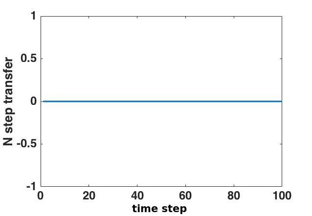
Example 1 revisited : For the three state example discussed in section 2, we compute the information transfer using our proposed definition of information transfer and the formula (16). In Fig. 4(a), we plot the information transfer over n𝑛n time steps and we notice that the information transfer from x1x2subscript𝑥1subscript𝑥2x_{1}\to x_{2} and x1x3subscript𝑥1subscript𝑥3x_{1}\to x_{3} are identically zero.

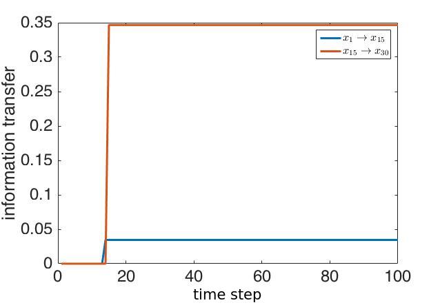
Example 2 revisited : We compute the information transfer from x1xksubscript𝑥1subscript𝑥𝑘x_{1}\to x_{k} and from xkxNsubscript𝑥𝑘subscript𝑥𝑁x_{k}\to x_{N} for k=15𝑘15k=15. Since, x1subscript𝑥1x_{1} is connected to xksubscript𝑥𝑘x_{k} through series of k𝑘k delays, as expected the information transfer Tx1xksubscript𝑇subscript𝑥1subscript𝑥𝑘T_{x_{1}\to x_{k}} is zero over n<k𝑛𝑘n<k time step and for n=k𝑛𝑘n=k the information transfer jumps from zero to non-zero value as shown in Fig. 4(b). Similarly information transfer from xkxNsubscript𝑥𝑘subscript𝑥𝑁x_{k}\to x_{N} also shows a sudden jump. This proves that our proposed definition of information transfer obeys the time constraints of transfer.
Refer to caption
Refer to caption
Figure 4: (a) N-step information transfer for example 1. (b) N-step information transfer for example 2.

4 Information Transfer in Linear Control Systems

In this section, we derive expression for information transfer in control dynamical system. In particular, we derive expressions for information transfer from state to output, input to state, and input to output. For the simplicity of discussion we also restrict our discussion to single input single output case.

We consider the following linear linear time invariant system with input and output.

z(t+1)=Az(t)+Bu(t)θ(t)=Cz(t)+ω(t)missing-subexpression𝑧𝑡1𝐴𝑧𝑡𝐵𝑢𝑡missing-subexpression𝜃𝑡𝐶𝑧𝑡𝜔𝑡\displaystyle\begin{aligned} &z(t+1)=Az(t)+Bu(t)\\ &\theta(t)=Cz(t)+\omega(t)\end{aligned} (33)

where zN𝑧superscript𝑁z\in\mathbb{R}^{N} are the states, AN×N𝐴superscript𝑁𝑁A\in\mathbb{R}^{N\times N}, B𝐵B and C𝐶C are of appropriate dimensions, u(t)𝑢𝑡u(t)\in\mathbb{R} is the input, θ𝜃\theta\in\mathbb{R} is output and ω(t)𝜔𝑡\omega(t) is the output noise, which is assumed to be zero mean i.i.d. Gaussian noise. For the simplicity of presentation, we will restrict our discussion to the case where the state space z𝑧z is split in only two subspace i.e., z=(x,y)𝑧superscriptsuperscript𝑥topsuperscript𝑦toptopz=(x^{\top},y^{\top})^{\top} and the inputs and outputs are one dimensional. With this assumption, we have following splitting of the A,B𝐴𝐵A,B, and C𝐶C matrices.

A=(AxAxyAyxAy),B=(BxBy),C=(CxCy)formulae-sequence𝐴matrixsubscript𝐴𝑥subscript𝐴𝑥𝑦subscript𝐴𝑦𝑥subscript𝐴𝑦formulae-sequence𝐵matrixsubscript𝐵𝑥subscript𝐵𝑦𝐶matrixsubscript𝐶𝑥subscript𝐶𝑦\displaystyle A=\begin{pmatrix}A_{x}&A_{xy}\\ A_{yx}&A_{y}\end{pmatrix},B=\begin{pmatrix}B_{x}\\ B_{y}\end{pmatrix},C=\begin{pmatrix}C_{x}&C_{y}\end{pmatrix} (34)

4.1 Information from Input to State

The evolution of the state x𝑥x is x=Axx+Axyy+Bxusuperscript𝑥subscript𝐴𝑥𝑥subscript𝐴𝑥𝑦𝑦subscript𝐵𝑥𝑢x^{\prime}=A_{x}x+A_{xy}y+B_{x}u. In deriving the formulas in this section, we think of the input u(t)𝑢𝑡u(t) as a i.i.d. Gaussian variable such that

E[u(t)u(t+k)]=0,kt and E[zu]=0.formulae-sequenceEdelimited-[]𝑢𝑡𝑢superscript𝑡𝑘top0for-all𝑘𝑡 and Edelimited-[]𝑧superscript𝑢top0\displaystyle\textnormal{E}[u(t)u(t+k)^{\top}]=0,\forall k\neq t\textnormal{ and }\textnormal{E}[zu^{\top}]=0.

Hence,

Σx|x=AxyΣxsAxy+BxΣuBxsubscriptΣconditionalsuperscript𝑥𝑥subscript𝐴𝑥𝑦superscriptsubscriptΣ𝑥𝑠superscriptsubscript𝐴𝑥𝑦topsubscript𝐵𝑥subscriptΣ𝑢superscriptsubscript𝐵𝑥top\displaystyle\Sigma_{x^{\prime}|x}=A_{xy}\Sigma_{x}^{s}A_{xy}^{\top}+B_{x}\Sigma_{u}B_{x}^{\top} (35)

where ΣxssuperscriptsubscriptΣ𝑥𝑠\Sigma_{x}^{s} is the Schur complement of ΣxsubscriptΣ𝑥\Sigma_{x} in ΣzsubscriptΣ𝑧\Sigma_{z} and ΣusubscriptΣ𝑢\Sigma_{u} is the covariance of the input at time t𝑡t.

When the input u𝑢u is held frozen,

Σx|x=AxyΣxsAxysuperscriptsubscriptΣconditionalsuperscript𝑥𝑥italic-u̸subscript𝐴𝑥𝑦superscriptsubscriptΣ𝑥𝑠superscriptsubscript𝐴𝑥𝑦top\displaystyle\Sigma_{x^{\prime}|x}^{\not{u}}=A_{xy}\Sigma_{x}^{s}A_{xy}^{\top} (36)

Hence the information transfer from u1subscript𝑢1u_{1} to x𝑥x is

Tux=12log|AxyΣxsAxy+BxΣuBx||AxyΣxsAxy|subscript𝑇𝑢𝑥12subscript𝐴𝑥𝑦superscriptsubscriptΣ𝑥𝑠superscriptsubscript𝐴𝑥𝑦topsubscript𝐵𝑥subscriptΣ𝑢superscriptsubscript𝐵𝑥topsubscript𝐴𝑥𝑦superscriptsubscriptΣ𝑥𝑠superscriptsubscript𝐴𝑥𝑦top\displaystyle T_{u\to x}=\frac{1}{2}\log\frac{|A_{xy}\Sigma_{x}^{s}A_{xy}^{\top}+B_{x}\Sigma_{u}B_{x}^{\top}|}{|A_{xy}\Sigma_{x}^{s}A_{xy}^{\top}|} (37)

where |||\cdot| is the determinant.

4.2 Information from State to Output

In this subsection, we look at the information transfer from the states of the system to the output of the control system. For simplicity, we only look at the information transfer from the entire state space z𝑧z to the output θ𝜃\theta. The general case of the information transfer from any state zisubscript𝑧𝑖z_{i} to any output θjsubscript𝜃𝑗\theta_{j} for a MIMO system can be dealt with in similar manner.

From the output equation, we have

Σθ|θ=CΣzC+Σω(CAΣzC)(CΣzC)1(CAΣzC)subscriptΣconditionalsuperscript𝜃𝜃𝐶subscriptΣsuperscript𝑧superscript𝐶topsubscriptΣ𝜔𝐶𝐴subscriptΣ𝑧superscript𝐶topsuperscript𝐶subscriptΣ𝑧superscript𝐶top1superscript𝐶𝐴subscriptΣ𝑧superscript𝐶toptop\displaystyle\Sigma_{\theta^{\prime}|\theta}=C\Sigma_{z^{\prime}}C^{\top}+\Sigma_{\omega}-(CA\Sigma_{z}C^{\top})(C\Sigma_{z}C^{\top})^{-1}(CA\Sigma_{z}C^{\top})^{\top}

where Σz=AΣzA+BΣuBsubscriptΣsuperscript𝑧𝐴subscriptΣ𝑧superscript𝐴top𝐵subscriptΣ𝑢superscript𝐵top\Sigma_{z^{\prime}}=A\Sigma_{z}A^{\top}+B\Sigma_{u}B^{\top} and ΣωsubscriptΣ𝜔\Sigma_{\omega} is the covariance of the output noise.

When z𝑧z is frozen, the output equation is

θ(t)=ω(t)subscript𝜃italic-z̸𝑡𝜔𝑡\displaystyle\theta_{\not{z}}(t)=\omega(t) (38)

Hence, Σθ|θ=ΣωsuperscriptsubscriptΣconditionalsuperscript𝜃𝜃italic-z̸subscriptΣ𝜔\Sigma_{\theta^{\prime}|\theta}^{\not{z}}=\Sigma_{\omega}.

So the transfer is

Tzθ=12log|Σθ|θ||Σω|subscript𝑇𝑧𝜃12subscriptΣconditionalsuperscript𝜃𝜃subscriptΣ𝜔\displaystyle T_{z\to\theta}=\frac{1}{2}\log\frac{|\Sigma_{\theta^{\prime}|\theta}|}{|\Sigma_{\omega}|}

where

Σθ|θ=CΣzC+Σω(CAΣzC)(CΣzC)1(CAΣzC)subscriptΣconditionalsuperscript𝜃𝜃𝐶subscriptΣsuperscript𝑧superscript𝐶topsubscriptΣ𝜔𝐶𝐴subscriptΣ𝑧superscript𝐶topsuperscript𝐶subscriptΣ𝑧superscript𝐶top1superscript𝐶𝐴subscriptΣ𝑧superscript𝐶toptop\displaystyle\Sigma_{\theta^{\prime}|\theta}=C\Sigma_{z^{\prime}}C^{\top}+\Sigma_{\omega}-(CA\Sigma_{z}C^{\top})(C\Sigma_{z}C^{\top})^{-1}(CA\Sigma_{z}C^{\top})^{\top}

4.3 Information from Input to Output

As before, we address the case of SISO systems for simplicity. We have

Σθ=CAΣzAC+CBΣuBCsuperscriptsubscriptΣ𝜃𝐶𝐴subscriptΣ𝑧superscript𝐴topsuperscript𝐶top𝐶𝐵subscriptΣ𝑢superscript𝐵topsuperscript𝐶top\displaystyle\Sigma_{\theta}^{\prime}=CA\Sigma_{z}A^{\top}C^{\top}+CB\Sigma_{u}B^{\top}C^{\top}

Hence,

Σθ|θ=CAΣzAC+CBΣuBc+Σω(CAΣzC)(CΣzC)1(CAΣzC)subscriptΣconditionalsuperscript𝜃𝜃𝐶𝐴subscriptΣ𝑧superscript𝐴topsuperscript𝐶top𝐶𝐵subscriptΣ𝑢superscript𝐵topsuperscript𝑐topsubscriptΣ𝜔𝐶𝐴subscriptΣ𝑧superscript𝐶topsuperscript𝐶subscriptΣ𝑧superscript𝐶top1superscript𝐶𝐴subscriptΣ𝑧superscript𝐶toptop\displaystyle\Sigma_{\theta^{\prime}|\theta}=CA\Sigma_{z}A^{\top}C^{\top}+CB\Sigma_{u}B^{\top}c^{\top}+\Sigma_{\omega}-(CA\Sigma_{z}C^{\top})(C\Sigma_{z}C^{\top})^{-1}(CA\Sigma_{z}C^{\top})^{\top} (39)

When u𝑢u is frozen, we have

z=Azθ=Cz+ωmissing-subexpressionsuperscript𝑧𝐴𝑧missing-subexpression𝜃𝐶𝑧𝜔\displaystyle\begin{aligned} &z^{\prime}=Az\\ &\theta=Cz+\omega\end{aligned} (40)

Hence,

Σθ|θ=CAΣzAC+Σω(CAΣzC)(CΣzC)1(CAΣzC)subscriptΣconditionalsuperscriptsubscript𝜃italic-u̸subscript𝜃italic-u̸𝐶𝐴subscriptΣ𝑧superscript𝐴topsuperscript𝐶topsubscriptΣ𝜔𝐶𝐴subscriptΣ𝑧superscript𝐶topsuperscript𝐶subscriptΣ𝑧superscript𝐶top1superscript𝐶𝐴subscriptΣ𝑧superscript𝐶toptop\displaystyle\Sigma_{\theta_{\not{u}}^{\prime}|\theta_{\not{u}}}=CA\Sigma_{z}A^{\top}C^{\top}+\Sigma_{\omega}-(CA\Sigma_{z}C^{\top})(C\Sigma_{z}C^{\top})^{-1}(CA\Sigma_{z}C^{\top})^{\top} (41)

Hence the transfer is

Tuθ=12log|Σθ|θ||Σθ|θ|subscript𝑇𝑢𝜃12subscriptΣconditionalsuperscript𝜃𝜃subscriptΣconditionalsuperscriptsubscript𝜃italic-u̸subscript𝜃italic-u̸\displaystyle T_{u\to\theta}=\frac{1}{2}\log\frac{|\Sigma_{\theta^{\prime}|\theta}|}{|\Sigma_{\theta_{\not{u}}^{\prime}|\theta_{\not{u}}}|} (42)

where Σθ|θsubscriptΣconditionalsuperscript𝜃𝜃\Sigma_{\theta^{\prime}|\theta} and Σθ|θsubscriptΣconditionalsuperscriptsubscript𝜃italic-u̸subscript𝜃italic-u̸\Sigma_{\theta_{\not{u}}^{\prime}|\theta_{\not{u}}} are given by equations (39) and (41) respectively.

4.4 Information Transfer in Feedback Control Systems
Refer to caption
Figure 5: Feedback control system

Information theory and feedback systems are interlinked and researchers have studied their interplay [19, 20, 21, 22]. Again, Massey [9] had shown that the feedback capacity (Cfb)subscript𝐶𝑓𝑏(C_{fb}) satisfies

Cfblimnmaxρ(Xn||Yn1)1nI(XnYn)\displaystyle C_{fb}\leq\lim_{n\to\infty}\max_{\rho(X^{n}||Y^{n-1})}\frac{1}{n}I(X^{n}\to Y^{n}) (43)

where ρ(Xn||Yn1)\rho(X^{n}||Y^{n-1}) is the conditional distribution of Xnsuperscript𝑋𝑛X^{n}, causally conditioned on Yn1superscript𝑌𝑛1Y^{n-1}. Again, in [23], it has been proved that in a feedback system, the Bode sensitivity transfer function from the output to the input is equal to the average directed information from the output (w)𝑤(w) to the input (u)𝑢(u), where the average directed information from the output to the input is defined as

limn1nI(wnun)subscript𝑛1𝑛𝐼superscript𝑤𝑛superscript𝑢𝑛\displaystyle\lim_{n\to\infty}\frac{1}{n}I(w^{n}\to u^{n}) (44)

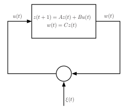
In this section, we consider the following feedback control system (figure 5)

z(t+1)=Az(t)+Bu(t)w(t)=Cz(t),u(t)=w(t)+ξ(t)missing-subexpression𝑧𝑡1𝐴𝑧𝑡𝐵𝑢𝑡missing-subexpressionformulae-sequence𝑤𝑡𝐶𝑧𝑡𝑢𝑡𝑤𝑡𝜉𝑡\displaystyle\begin{aligned} &z(t+1)=Az(t)+Bu(t)\\ &w(t)=Cz(t),\;\;u(t)=w(t)+\xi(t)\end{aligned} (45)

and we are interested in computing information flow from output to input of the feedback control system i.e., Twusubscript𝑇𝑤𝑢T_{w\to u}. This is the information transfer from the plant to itself. Towards this goal we write the feedback control system as follows:

z(t+1)=(A+BC)z(t)+Bξ(t)𝑧𝑡1𝐴𝐵𝐶𝑧𝑡𝐵𝜉𝑡\displaystyle z(t+1)=(A+BC)z(t)+B\xi(t)
w(t)=Cz(t),u(t)=w(t)+ξ(t)formulae-sequence𝑤𝑡𝐶𝑧𝑡𝑢𝑡𝑤𝑡𝜉𝑡\displaystyle w(t)=Cz(t),\;\;\;u(t)=w(t)+\xi(t) (46)

Hence, H(ρ(u|u))=H(ρ(ξ))subscript𝐻italic-w̸𝜌conditionalsuperscript𝑢𝑢𝐻𝜌superscript𝜉H_{\not{w}}(\rho(u^{{}^{\prime}}|u))=H(\rho(\xi^{{}^{\prime}})). With this, and theorem (5), next we show that the Bode sensitivity transfer function, 𝒮𝒮\mathcal{S}, from w𝑤w to u𝑢u is same as the average information transfer from w𝑤w to u𝑢u.

Theorem 11.
T¯xy=1212log|𝒮(ej2πθ)|dθ=i=1mlog|λi(Au)|subscript¯𝑇𝑥𝑦superscriptsubscript1212𝒮superscript𝑒𝑗2𝜋𝜃𝑑𝜃superscriptsubscript𝑖1𝑚subscript𝜆𝑖subscript𝐴𝑢\displaystyle\bar{T}_{x\to y}=\int_{-\frac{1}{2}}^{\frac{1}{2}}\log|\mathcal{S}(e^{j2\pi\theta})|d\theta=\sum_{i=1}^{m}\log|\lambda_{i}(A_{u})|

where λi(Au)subscript𝜆𝑖subscript𝐴𝑢\lambda_{i}(A_{u}) are the unstable eigenvalues of the open loop system.

Proof.

From theorem (5), we have

T¯xy=limT1Ti=1T(Txy)0i=limT1T[H(uT)H(uT)]=limT1T[H(uT)H(ξT)]=limT12Tlog|ΣuT||ΣξT|=1212log|u(ej2πθ)|2|ξ(ej2πθ)|2dθ=1212log|𝒮(ej2πθ)|dθ=i=1mlog|λi(Au)|missing-subexpressionsubscript¯𝑇𝑥𝑦subscript𝑇1𝑇superscriptsubscript𝑖1𝑇superscriptsubscriptsubscript𝑇𝑥𝑦0𝑖missing-subexpressionabsentsubscript𝑇1𝑇delimited-[]𝐻superscript𝑢𝑇subscript𝐻italic-w̸superscript𝑢𝑇subscript𝑇1𝑇delimited-[]𝐻superscript𝑢𝑇𝐻superscript𝜉𝑇missing-subexpressionabsentsubscript𝑇12𝑇subscriptΣsuperscript𝑢𝑇subscriptΣsuperscript𝜉𝑇superscriptsubscript1212superscript𝑢superscript𝑒𝑗2𝜋𝜃2superscript𝜉superscript𝑒𝑗2𝜋𝜃2𝑑𝜃missing-subexpressionabsentsuperscriptsubscript1212𝒮superscript𝑒𝑗2𝜋𝜃𝑑𝜃superscriptsubscript𝑖1𝑚subscript𝜆𝑖subscript𝐴𝑢\displaystyle\begin{aligned} &\bar{T}_{x\to y}=\lim_{T\to\infty}\frac{1}{T}\sum_{i=1}^{T}(T_{x\to y})_{0}^{i}\\ &=\lim_{T\to\infty}\frac{1}{T}[H(u^{T})-H_{\not{w}}(u^{T})]=\lim_{T\to\infty}\frac{1}{T}[H(u^{T})-H(\xi^{T})]\\ &=\lim_{T\to\infty}\frac{1}{2T}\log\frac{|\Sigma_{u^{T}}|}{|\Sigma_{\xi^{T}}|}=\int_{-\frac{1}{2}}^{\frac{1}{2}}\log\frac{|u(e^{j2\pi\theta})|^{2}}{|\xi(e^{j2\pi\theta})|^{2}}d\theta\\ &=\int_{-\frac{1}{2}}^{\frac{1}{2}}\log|\mathcal{S}(e^{j2\pi\theta})|d\theta=\sum_{i=1}^{m}\log|\lambda_{i}(A_{u})|\end{aligned}

where λi(Au)subscript𝜆𝑖subscript𝐴𝑢\lambda_{i}(A_{u}) are the unstable poles of A𝐴A.

Hence, the average directed information and average information transfer are the same for the above feedback control system. This theorem, along with the fact that the channel capacity of a feedback channel is related to directed information, presents further evidence that our formulation of information transfer, though developed from dynamical systems point of view, is consistent with already existing concepts in information theory and control theory. We feel this will allow us to study the concepts of information theory, control theory and dynamical systems from a more fundamental and common point of view.

Example 12.

Consider the feedback system given in figure 5 with

A=(4200.7),B=(10),C=[3.50]formulae-sequence𝐴4200.7formulae-sequence𝐵10𝐶delimited-[]3.50\displaystyle\begin{aligned} A=\left(\begin{array}[]{cc}4&2\\ 0&0.7\end{array}\right),\quad B=\left(\begin{array}[]{c}1\\ 0\end{array}\right),\quad C=[\begin{array}[]{cc}-3.5&0\end{array}]\end{aligned}

We also assume that the noise ω𝜔\omega is i.i.d. zero mean unit variance Gaussian white noise.
Refer to caption
Refer to caption
Figure 6: (a) N-step information transfer; (b) Average information transfer and average directed information

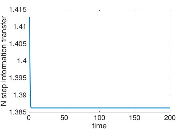
The open loop system has unstable pole at 444. Hence the Bode integral of the sensitivity transfer function is log(4)=1.386341.3863\log(4)=1.3863. Figure 6(a) shows the N-step information transfer from the output of the system to the input of the system. The steady state value of the information transfer is 1.38631.38631.3863. Similarly, the average information transfer from the output to the input is also 1.38631.38631.3863. This is shown in figure 6(b). In this figure we also plot the average directed information transfer from the output to input. Here again we observe that the average information transfer converges to the Bode integral of the sensitivity transfer function much faster than the average directed information.

5 Information Transfer and Structural Controllability and Observability

Structural controllability was developed by [24], and is a weaker notion of controllability, where a system is said to structurally controllable, if either the system is controllable or is controllable when the non-zero entries of the system matrix are perturbed so that the perturbed system becomes controllable. Associated with a system

z(t+1)=Az(t)+ξ(t),zNformulae-sequence𝑧𝑡1𝐴𝑧𝑡𝜉𝑡𝑧superscript𝑁\displaystyle z(t+1)=Az(t)+\xi(t),\quad z\in\mathbb{R}^{N} (47)

is a directed graph Z=(Vz,Ez)𝑍subscript𝑉𝑧subscript𝐸𝑧Z=(V_{z},E_{z}) where Vz={zi|i=1,,N}subscript𝑉𝑧conditional-setsubscript𝑧𝑖𝑖1𝑁V_{z}=\{z_{i}|i=1,\ldots,N\} is the node set and Ezsubscript𝐸𝑧E_{z} is the edge set, such that there is directed edge from zisubscript𝑧𝑖z_{i} to zjsubscript𝑧𝑗z_{j} iff jith𝑗superscript𝑖𝑡{ji}^{th} entry of A𝐴A is non-zero. Now if a single control input is placed at node k𝑘k, then one can construct an extended graph G=(V,E)𝐺𝑉𝐸G=(V,E), with one extra node u𝑢u and one extra edge from u𝑢u to zksubscript𝑧𝑘z_{k}. With this, the system is said to structurally controllable if all the nodes of the extended graph can be reached from node u𝑢u [25]. Since u𝑢u is directly connected to zksubscript𝑧𝑘z_{k}, one can say that the system, with input at zksubscript𝑧𝑘z_{k}, is structurally controllable if there exists paths to all the nodes of Z𝑍Z from zksubscript𝑧𝑘z_{k}.

In this section we show that if information transfer from the input to all the nodes is non-zero, then the system is structurally controllable. Note that in this section, by information transfer, we will mean n𝑛n-step information transfer for n>0𝑛subscriptabsent0n\in\mathbb{Z}_{>0}.

Theorem 13.

If the k𝑘k-step information transfer from state zisubscript𝑧𝑖z_{i} to zjsubscript𝑧𝑗z_{j} of system (47) is non-zero for some k>0𝑘subscriptabsent0k\in\mathbb{Z}_{>0}, then there is a directed path from node zisubscript𝑧𝑖z_{i} to zjsubscript𝑧𝑗z_{j} in the corresponding directed graph for the system.

Proof.

We prove this by contrapositive argument. Without loss of generality, we assume i=2𝑖2i=2 and j=1𝑗1j=1. Suppose there is no path from z2subscript𝑧2z_{2} to z1subscript𝑧1z_{1}. Hence, [Ak]12=0subscriptdelimited-[]superscript𝐴𝑘120[A^{k}]_{12}=0 for all k𝑘k\in\mathbb{Z} 222Here [Ak]ijsubscriptdelimited-[]superscript𝐴𝑘𝑖𝑗[A^{k}]_{ij} means the ijth𝑖superscript𝑗𝑡ij^{th} entry of Aksuperscript𝐴𝑘A^{k} . We show that in this case the k𝑘k-step information transfer from z2subscript𝑧2z_{2} to z1subscript𝑧1z_{1} is zero for all k𝑘k\in\mathbb{Z}. The evolution of the states can be written as

z(k)=Akz(0)+Ak1ξ(0)++ξ(k1)𝑧𝑘superscript𝐴𝑘𝑧0superscript𝐴𝑘1𝜉0𝜉𝑘1\displaystyle z(k)=A^{k}z(0)+A^{k-1}\xi(0)+\ldots+\xi(k-1) (48)

Hence,

z1(k)subscript𝑧1𝑘\displaystyle z_{1}(k) =\displaystyle= j=1,j2N[Ak](1j)zj(0)+j=1,j2N[Ak1](1j)ξj(0)superscriptsubscriptformulae-sequence𝑗1𝑗2𝑁subscriptdelimited-[]superscript𝐴𝑘1𝑗subscript𝑧𝑗0superscriptsubscriptformulae-sequence𝑗1𝑗2𝑁subscriptdelimited-[]superscript𝐴𝑘11𝑗subscript𝜉𝑗0\displaystyle\sum_{j=1,j\neq 2}^{N}[A^{k}]_{(1j)}z_{j}(0)+\sum_{j=1,j\neq 2}^{N}[A^{k-1}]_{(1j)}\xi_{j}(0) (49)
++ξ1(k)subscript𝜉1𝑘\displaystyle+\ldots+\xi_{1}(k)

since [Ak]12=0subscriptdelimited-[]superscript𝐴𝑘120[A^{k}]_{12}=0 and when z2subscript𝑧2z_{2} is held frozen, we have

z1(k)subscript𝑧1not-2𝑘\displaystyle z_{1\not{2}}(k) =\displaystyle= j=1,j2N[Ak](1j)zj(0)+j=1,j2N[Ak1](1j)ξj(0)superscriptsubscriptformulae-sequence𝑗1𝑗2𝑁subscriptdelimited-[]superscriptsubscript𝐴not-2𝑘1𝑗subscript𝑧𝑗0superscriptsubscriptformulae-sequence𝑗1𝑗2𝑁subscriptdelimited-[]superscriptsubscript𝐴not-2𝑘11𝑗subscript𝜉𝑗0\displaystyle\sum_{j=1,j\neq 2}^{N}[A_{\not{2}}^{k}]_{(1j)}z_{j}(0)+\sum_{j=1,j\neq 2}^{N}[A_{\not{2}}^{k-1}]_{(1j)}\xi_{j}(0) (50)
++ξ1(k)subscript𝜉1𝑘\displaystyle+\ldots+\xi_{1}(k)

where Asubscript𝐴not-2A_{\not{2}} is the system matrix when z2subscript𝑧2z_{2} is held frozen, that is Asubscript𝐴not-2A_{\not{2}} is obtained from A𝐴A by deleting the second row and second column of A𝐴A.

Now,

[A2](1j)=i=1Na1iaij=a12a2j+i2a1iaijsubscriptdelimited-[]superscript𝐴21𝑗superscriptsubscript𝑖1𝑁subscript𝑎1𝑖subscript𝑎𝑖𝑗subscript𝑎12subscript𝑎2𝑗subscript𝑖2subscript𝑎1𝑖subscript𝑎𝑖𝑗\displaystyle[A^{2}]_{(1j)}=\sum_{i=1}^{N}a_{1i}a_{ij}=a_{12}a_{2j}+\sum_{i\neq 2}a_{1i}a_{ij}
=i2a1iaij=[A2]1jabsentsubscript𝑖2subscript𝑎1𝑖subscript𝑎𝑖𝑗subscriptdelimited-[]superscriptsubscript𝐴not-221𝑗\displaystyle=\sum_{i\neq 2}a_{1i}a_{ij}=[A_{\not{2}}^{2}]_{1j} (51)

since a12=0subscript𝑎120a_{12}=0.

Similarly,

[A3]1j=[A2A]1j=[A2A]1j=i(a2)1iaij=subscriptdelimited-[]superscript𝐴31𝑗subscriptdelimited-[]superscript𝐴2𝐴1𝑗subscriptdelimited-[]subscript𝐴2𝐴1𝑗subscript𝑖subscriptsubscript𝑎21𝑖subscript𝑎𝑖𝑗absent\displaystyle[A^{3}]_{1j}=[A^{2}A]_{1j}=[A_{2}A]_{1j}=\sum_{i}(a_{2})_{1i}a_{ij}=
(a2)12a2j+i2(a2)1iaij=i2(a2)1iaij=[A3]1jsubscriptsubscript𝑎212subscript𝑎2𝑗subscript𝑖2subscriptsubscript𝑎21𝑖subscript𝑎𝑖𝑗subscript𝑖2subscriptsubscript𝑎21𝑖subscript𝑎𝑖𝑗subscriptdelimited-[]superscriptsubscript𝐴not-231𝑗\displaystyle(a_{2})_{12}a_{2j}+\sum_{i\neq 2}(a_{2})_{1i}a_{ij}=\sum_{i\neq 2}(a_{2})_{1i}a_{ij}=[A_{\not{2}}^{3}]_{1j}

since [A2]12=(a2)12=0subscriptdelimited-[]superscript𝐴212subscriptsubscript𝑎2120[A^{2}]_{12}=(a_{2})_{12}=0. Let [Al]1j=[Al]1jsubscriptdelimited-[]superscript𝐴𝑙1𝑗subscriptdelimited-[]superscriptsubscript𝐴not-2𝑙1𝑗[A^{l}]_{1j}=[A_{\not{2}}^{l}]_{1j} for some l>0𝑙subscriptabsent0l\in\mathbb{Z}_{>0}. Then

[Al+1]1j=[AlA]1j=[AlA]1j=i(al)1iaij=subscriptdelimited-[]superscript𝐴𝑙11𝑗subscriptdelimited-[]superscript𝐴𝑙𝐴1𝑗subscriptdelimited-[]subscript𝐴𝑙𝐴1𝑗subscript𝑖subscriptsubscript𝑎𝑙1𝑖subscript𝑎𝑖𝑗absent\displaystyle[A^{l+1}]_{1j}=[A^{l}A]_{1j}=[A_{l}A]_{1j}=\sum_{i}(a_{l})_{1i}a_{ij}=
(al)12a2j+i2(al)1iaij=i2(al)1iaij=[Al+1]1jsubscriptsubscript𝑎𝑙12subscript𝑎2𝑗subscript𝑖2subscriptsubscript𝑎𝑙1𝑖subscript𝑎𝑖𝑗subscript𝑖2subscriptsubscript𝑎𝑙1𝑖subscript𝑎𝑖𝑗subscriptdelimited-[]superscriptsubscript𝐴not-2𝑙11𝑗\displaystyle(a_{l})_{12}a_{2j}+\sum_{i\neq 2}(a_{l})_{1i}a_{ij}=\sum_{i\neq 2}(a_{l})_{1i}a_{ij}=[A_{\not{2}}^{l+1}]_{1j}

Hence, [Ak]1j=[Ak]1jsubscriptdelimited-[]superscript𝐴𝑘1𝑗subscriptdelimited-[]superscriptsubscript𝐴not-2𝑘1𝑗[A^{k}]_{1j}=[A_{\not{2}}^{k}]_{1j} for all k𝑘k\in\mathbb{Z}. Hence from (49) and (50), z1(k)=z1(k)subscript𝑧1𝑘subscript𝑧1not-2𝑘z_{1}(k)=z_{1\not{2}}(k). So,

H(z1(k)|z1(k1)z1(0))𝐻conditionalsubscript𝑧1𝑘subscript𝑧1𝑘1subscript𝑧10\displaystyle H(z_{1}(k)|z_{1}(k-1)\ldots z_{1}(0))
=H2(z1(k)|z1(k1)z1(0)).absentsubscript𝐻subscriptitalic-z̸2conditionalsubscript𝑧1𝑘subscript𝑧1𝑘1subscript𝑧10\displaystyle=H_{\not{z}_{2}}(z_{1}(k)|z_{1}(k-1)\ldots z_{1}(0)).

Hence [Tz2z1]0k=0superscriptsubscriptdelimited-[]subscript𝑇subscript𝑧2subscript𝑧10𝑘0[T_{z_{2}\to z_{1}}]_{0}^{k}=0 for all k𝑘k\in\mathbb{Z}. Hence, if there is non zero information transfer from z2subscript𝑧2z_{2} to z1subscript𝑧1z_{1}, then there exists a directed path from z2subscript𝑧2z_{2} to z1subscript𝑧1z_{1}. ∎

Theorem 14.

If the information transfer from the input to all the states are non-zero, then the system is structurally controllable.

Proof.

We consider the extended graph associated with the dynamical system and consider the input node as an extra state. From theorem (13), if the information transfer from the input to any state zisubscript𝑧𝑖z_{i} is non-zero, then there exists a path from the input node to the node zisubscript𝑧𝑖z_{i} in the directed graph associated with the system. So, if the information transfer from the input to all the states is non zero, then there exists directed paths from the input node to all the other nodes in the directed graph associated with the system and hence the system is input reachable and hence is structurally controllable. ∎

Results for structural observability follows from duality and can be stated as

Theorem 15.

If the information transfer from all the states to the output is non zero, then the system is structurally observable.

Here we have proved the result for structural controllability for SISO case, but the result for MIMO case is similar.

6 Conclusion

In this paper, we discussed how directed information fails to capture the causal structure in a dynamical system and provided a new measure of causality based on a new definition of information transfer and have shown that it captures the intuitions of causality. The new definition of information, which is based on dynamical system setting, has been generalized to define information transfer between the various signals in a control dynamical system. This generalization resulted in connecting the information transfer with Bode integral of the sensitivity transfer function from the output to the input in a feedback control system.

References

  • [1] G. V. Steeg and A. Galstyan, “Information transfer in social media,” in Proceedings of the 21st international conference on World Wide Web, New York, NY, 2012, pp. 509–518.
  • [2] O. Sporns, The networks of the brain.   MIT Press, 2010.
  • [3] D. J. S. A. Rao, A. O. Hero and J. D. Engel, “Motif discovery in tissue-specific regulatory sequences using directed information.” in EURASIP J. on Bioinformatics and Systems Biology, 2007.
  • [4] ——, “Inference of biologically relevant gene influence networks using the directed information criterion.” in In proc. ICASSP, Toulouse, France, 2006.
  • [5] C.W.J. Granger, “Investigating causal relations by econometrics models and cross-spectral methods,” Econometrica, vol. 37, no. 3, pp. 424–438, 1969.
  • [6] C. A. Sims, “Money, income and causality,” American Economic Review, vol. 62, pp. 540–552, 1972.
  • [7] C. W. J. Granger, “Testing for causality,” Journal of Economic Dynamics and Control, vol. 2, pp. 329–352, 1980.
  • [8] H. Touchette and S. Lloyd, “Information-theoretic approach to the study of control systems,” Physica A: Statistical Mechanics and its Applications, vol. 331, no. 1, pp. 140–172, 2004.
  • [9] J. L. Massey, “Causality, feedback and directed information.” in Proc. Intl. Symp. on Info. th. and its Applications, Waikiki, Hawai, USA, 1990.
  • [10] G. Kramer, “Directed information for channels with feedback,” in PhD Thesis, Swiss Federal Institute of Technology Zurich, 1998.
  • [11] T. Schreiber, “Measuring information transfer,” Physical Review Letters, vol. 85, no. 2, pp. 461–464, July, 2000.
  • [12] X. S. Liang and R. Kleeman, “Information transfer between dynamical system components,” Physical Review Letters, vol. 95, p. 244101, 2005.
  • [13] X. S. Liang, “Local predictability and information flow in complex dynamical systems,” Physica D, vol. 248, pp. 1–15, 2013.
  • [14] X. S. Liang and R. Kleeman, “A rigorous formalism of information transfer between dynamical system components. I. Discrete mapping,” Physica D, vol. 231, pp. 1–9, 2007.
  • [15] A. J. Majda and J. Harlim, “Information transfer between subspace of complex dynamical systems,” PNAS, vol. 104, no. 23, pp. 9558–9563, 2007.
  • [16] S. Sinha and U. Vaidya, “Formalism for information transfer in dyamical networks,” 54th IEEE Conference on Decision and Control, Osaka, Japan, pp. 5731 – 5736, 2015.
  • [17] H. Marko, “The bidirectional communication theory- a generalization. of information theory,” IEEE Transaction on Communications, vol. Com - 21, no. 12, pp. 1345–1351, Dec, 1973.
  • [18] J. A. Costanzo and J. Dunstan, “A survey of causality and directed information,” 2014.
  • [19] W. S. Wong and R. W. Brockett, “Systems with finite communication bandwidth constraints. ii. stabilization with limited information feedback,” Automatic Control, IEEE Transactions on, vol. 44, no. 5, pp. 1049–1053, 1999.
  • [20] S. Tatikonda, A. Sahai, and S. Mitter, “Stochastic linear control over a communication channel,” Automatic Control, IEEE Transactions on, vol. 49, no. 9, pp. 1549–1561, 2004.
  • [21] D. Li and N. Hovakimyan, “Bode-like integral for continuous-time closed-loop systems in the presence of limited information,” Automatic Control, IEEE Transactions on, vol. 58, no. 6, pp. 1457–1469, 2013.
  • [22] S. Tatikonda and S. Mitter, “Control over noisy channels,” Automatic Control, IEEE Transactions on, vol. 49, no. 7, pp. 1196–1201, 2004.
  • [23] N. Elia, “When bode meets shannon: Control-oriented feedback communication schemes,” Automatic Control, IEEE Transactions on, vol. 49, no. 9, pp. 1477–1488, 2004.
  • [24] C. T. Lin, “Structural controllability,” Automatic Control, IEEE Transactions on, vol. 19, no. 3, pp. 201–208, 1974.
  • [25] D. D. Siljak, Decentralized control of complex systems.   Courier Corporation, 2011.