Coda reconstruction from cross-correlation of a diffuse field on thin elastic plates

Abstract

This study contributes to the evaluation of the robustness and accuracy of Green’s function reconstruction from cross-correlation of strongly dispersed reverberated signals, with disentangling of the respective roles of ballistic and reverberated (’coda’) contributions. We conduct a suite of experiments on a highly reverberating thin duralumin plate, where an approximately diffuse flexural wavefield is generated by taking advantage of the plate reverberation and wave dispersion. A large number of impulsive sources that cover the whole surface of the plate are used to validate ambient-noise theory through comparison of the causal and anticausal (i.e., positive- and negative-time) terms of the cross-correlation to one another, and to the directly measured Green’s function. To quantify the contribution of the ballistic and coda signals, the cross-correlation integral is defined over different time windows of variable length, and the accuracy of the reconstructed Green’s function is studied as a function of the initial and end times of the integral. We show that even cross-correlations measured over limited time windows converge to a significant part of the Green’s function. Convergence is achieved over a wide time window, which includes not only direct flexural-wave arrivals, but also the multiply reverberated coda. We propose a model, based on normal-mode analysis that relates the similarity between the cross-correlation and the Green’s function to the statistical properties of the plate. We also determine quantitatively how incoherent noise degrades the estimation of the Green’s function.

I Introduction

In parallel with the striking demonstration that cross-correlation of diffuse ambient noise recorded at two points can lead to recovery of the exact Green’s function between the two receivers Weaver2001 , the spatio-temporal correlation between a set of receivers in the presence of an impulsive source has been investigated. The results were particularly conclusive at the seismic scale, where coda-wave interferometry Snieder2002 was used to monitor highly scattering media with unprecedented accuracy. When averaged over a significant number of regional earthquakes, the cross-correlation of the coda waves also showed the possibility of recovering the Rayleigh surface waves between seismic sensors spread across Mexico Campillo2003 . The present paper aims to quantify the convergence of the correlation function toward the Green’s function at the laboratory scale in a two-dimensional thin-plate configuration. This property is derived from the formulation of the Ward identity when the propagation medium is covered with incoherent sources. When generalized to continuous ambient noise (instead of one or a set of impulsive sources), the cross-correlation theorem has resulted in both imaging and monitoring applications in a variety of fields, such as ultrasonics (e.g., Lobkis2001 ), helioseismology (e.g., Rickett1999 ), ocean acoustics (e.g., Roux2004 ), seismology from the regional to the global scale (e.g., Campillo2014 ; Boschi2015 ), medical imaging (e.g., Sabra2007 ), and structural engineering (e.g., Sabra2008 ).

If the Green’s function of the medium is to be reconstructed using this method, the diffuse incident field should result from the superposition of either decorrelated isotropic plane waves Wapenaar2005 or uniformly distributed noise sources Weaver2004 . While the first condition here is only valid in open media, the second one assumes that the anelastic attenuation is uniform within the medium of propagation. In both cases, it can be shown that the time derivative of the field cross-correlations between two points coincides with the difference between the ’causal’ and ’anticausal’ impulse responses; i.e., the Green’s function between the two points.

In practice, these conditions are only partially fulfilled. The mismatch between the cross-correlation and the Green’s function for a real noise source distribution is a measure of the accuracy of the method. The mismatch in homogeneous open media can be straightforwardly deduced from geometrical considerations of the source distribution Roux2005 . In complex random media, only statistical quantities can be inferred, and a mismatch appears as a fluctuation of the cross-correlation. In the case of multiple scattering media, these fluctuations can be relatively well predicted from a shot-noise model Larose2008 . However, only the use of multiple-scattering wave theory leads to fully consistent results Tiggelen2003 ; Rosny2013 .

Only a few studies have been devoted to the interferometric reconstruction of Green’s functions in bounded media. The related theory is, however, relevant to room acoustics Nowakowski2015 and passive structural health monitoring Sabra2008 ; Chehami2015 . In thin plates, the dispersion relation for noise generated by an air jet has been recovered Larose2007 . More recently, an experimental and numerical study was also conducted to determine the role of the ballistic and coda part on the cross-correlation when the source distribution was circular and uniformColombi2014 . Our study here follows Duroux et al. Duroux2010 , who investigated the convergence of the cross-correlation of vibrational waves in a thin aluminum plate. A heuristic shot-noise model introduced by Larose et al. Larose2008 was used to interpret the results.

Here, similar to Duroux2010 , the use of a Doppler vibrometer and the reciprocity theorem allows a very flexible study of the effects of the source distribution on the cross-correlation. The set-up allows the comparison of the cross-correlation result with the transient response that is estimated with an active source. We also study the symmetry of the correlation, because this is often an experimental proxy for the convergence toward the Green’s function.

We also cross-correlate a part of the multiply reflected wave (’coda’) instead of the entire reverberating time. The results are analyzed through modal decomposition of the cross-correlation over the eigen vibrational modes of the plate. This modal approach leads to consistent modeling of the cross-correlation that is governed by different regimes. When the number of sources is large enough, the model shows that even with a very short part of the coda, a perfect estimation of the Green’s function can be obtained. On the other hand, the similarity coefficient with a single source can be as small as a factor of $1/\sqrt{3}$ when the entire signal is correlated. The effects of uncorrelated noise (e.g., electronic noise) are also analyzed.

This paper is structured as follows: section II introduces the cross-correlation for flexural waves, and section III describes the experimental set-up and how the cross-correlation is built using the reciprocity theorem. In section IV, a preliminary study is proposed in terms of the symmetry of the Green’s function reconstruction, and relates this to the signal-to-noise ratio. In section V, the quantitative similarity between the direct impulse response and that obtained via cross-correlation of passive signals is studied. Section VI is devoted to an estimation of the similarity coefficient when cross-correlation is performed on only a part of the coda and a finite number of sources. Finally, the effects of uncorrelated noise on the correlation process are taken into account.

II Interferometry with Lamb waves

The cross-correlation theorem holds under the hypothesis of a diffuse wavefield. We assume here the definition of ’diffuse’ as given by Kinsler1999 : a wavefield is diffuse if all of the propagation directions have equal probability. This is approximately achieved in practice if the sources are distributed with equal probability with respect to the position, and/or if the recordings are very long in time in the presence of scattering and/or reverberation.
In the present experiments, we record the guided plate waves, which are known as Lamb waves. Lamb waves propagate according to two modes: symmetric and antisymmetric Royer2000 . At low frequency, the fundamental antisymmetric and dispersive Lamb mode ($A_{0}$) dominates the vertical plate displacements. According to the Kirchhoff-Love hypothesisVentsel2001 , the Green’s function ($G$) of the $A_{0}$ or flexural mode is the solution to the equation of motion associated with an impulsive point source,

$$D{\Delta^{2}}G(\textbf{r}-\textbf{r}_{0},t)+{\rho_{s}}(\frac{\partial^{2}G(\textbf{r}-\textbf{r}_{0},t)}{\partial{t}^{2}}+\frac{1}{\tau_{a}}\frac{\partial{G(\textbf{r}-\textbf{r}_{0},t)}}{\partial{t}})=-\delta(\textbf{r}_{0})\delta(t),$$ (1)

where $\Delta^{2}$ is the biLaplacian operator that is defined as the squared Laplacian, ${\rho_{s}}$ is the surface density of the plate, $\tau_{a}$ is the attenuation time, r is the position vector, $t$ is the time, and $D=h^{3}E/12(1-\nu^{2})$ is the bending stiffness, where $E$ and $\nu$ are the Young’s modulus and Poisson’s ratio, respectively, and $h$ is the thickness of the plate Fahy2007 . If the signal is generated by $N$ point sources of identical power spectral density $S(\omega)$, the Fourier transform of the cross-correlation estimated from a record of duration $\Delta T$ is given by

$$C(\textbf{r}_{l}^{R},\textbf{r}_{l^{\prime}}^{R},\omega)=\Delta T\sum_{k=1}^{N}G(\textbf{r}_{l}^{R},\textbf{r}_{k}^{S},\omega)G^{*}(\textbf{r}_{l^{\prime}}^{R},\textbf{r}_{k}^{S},\omega)S(\omega),$$ (2)

where $G^{*}$ is the complex conjugate of $G$, $\textbf{r}_{l}^{R}$ and $\textbf{r}_{k}^{S}$ are the $l$-th receiver position and the $k$-th source position, respectively. According to Chehami2014 , the cross-correlation is related to the imaginary part of the Green’s function by

$$C(\textbf{r}_{l}^{R},\textbf{r}_{l^{\prime}}^{R},\omega)=\frac{\Delta TS(\omega){N\tau_{a}}}{\rho_{s}\omega A}ImG{(\textbf{r}_{l}^{R},\textbf{r}_{l^{\prime}}^{R},\omega)}+Q(\omega)$$ (3)

where $A$ is the plate area, and the deviation $Q(\omega)$ can be caused, in particular, by non-uniformities in the source distribution, as well as by instrumental error. Equation (3) shows that the Green’s function associated with two locations $\textbf{r}_{l}^{R}$ and $\textbf{r}_{l^{\prime}}^{R}$ where sensors are deployed can be reconstructed by cross-correlation of the ambient recordings made by the two sensors, provided that the ambient noise is diffuse Chehami2014 .

III Plate experiments

III.1 Set-up

The experimental set-up consists of a homogeneous duralumin plate of 50 by 60 by 0.3 cm, with five piezoelectric transducers attached to the plate using instant glue (Fig. 1). There are neither significant material heterogeneities within the plate, nor scattering obstacles attached to it. The temperature of the room is controlled by an air conditioning system. We measured the room temperature continuously during the experiment and no significant variation was observed. All of the transducers are located at a minimum distance of 10 cm from the sides of the plate. Instead of a short pulse, a linear ’chirp’ in the frequency band of 100 Hz to 40,000 Hz with the rate of frequency change of 39900 Hz/s is sent via these transducers. The transducers are made of a 200$\mu$m-thick ceramic piezoelectric disk adhered to a thin 20mm-diameter and 200$\mu$m-thick metallic disk. Effect of such a transducer on the propagation is limited because total thickness of the transducer is only 13% of the plate thickness (the mass of the transducer equals 0.5g). On the other side of the plate, the vertical displacement induced by the vibration (i.e., Lamb waves) is scanned with a laser vibrometer. Since the higher Lamb modes ($A_{1}$,$S_{1}$, $A_{2}$, $S_{2}$, …) have a minimum cut-off frequency of 500 KHz, within our frequency band of interest, we can only generate the fundamental modes $A_{0}$, $S_{0}$ and $SH$ Lamb modes. Moreover, because we are working at less than a tenth of the cut-off frequency, the displacements recorded by the vibrometer are dominated by the $A_{0}$ mode. The latter, dubbed “flexural-plate mode” in the field of structural acoustics is very dispersive. Indeed, between 100 Hz to 40000 Hz, the phase velocity ranges between 17 m/s to 1000 m/s (i.e., wavelength between 170 to 25 mm). The group velocity has almost twice the value of the phase velocity. At such low frequency range, propagation of the $A_{0}$ mode is well described by Eq.  (1). Note that in this frequency range, Kirchhoff-Love model holds.

Figure 1: Experimental set-up, consisting of a duralumin plate and five piezoelectric transducers. The normal displacement of the plate is measured using a laser vibrometer placed on a two-dimensional motor and at the points marked by the black circles.

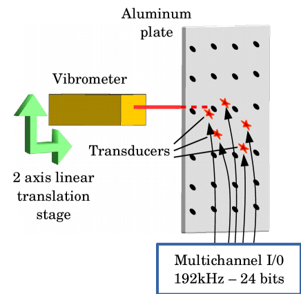
Recorded signal is cross-correlated with the chirp to extract the impulse response with the best signal-to-noise ratio.

III.2 Fundamental properties of the observed signal

Laser vibrometer scans are performed on a grid of about 2,500 regularly spaced locations (with a uniform distance of 1 cm between two points along the x and y plate directions), as qualitatively illustrated in Figure 1. An example of the recorded signals after chirp pulse compression is shown in Figure 2. Based on the reciprocity theorem (e.g., Aki1980 ), from now on we think of our readings as virtually emitted at the locations scanned by the vibrometer, and virtually recorded at transducer locations. This allows the simulation of the effects of a wide variety of source distributions.

Figure 2: (A) Example of the Lamb waves recorded by a transducer after pulse compression of the emitted chirp signal. The source-receiver distance is about 21 cm. The inset illustrates the envelope of the intensity of the signal (solid line) and the exponential fit according to $exp(-t/\tau_{a})$ (dashed line), as a semilog scale. The attenuation time ($\tau_{a}$) is 9 ms. Data at negative time gives a sense of the noise level. (B) Power spectrum of the raw signal (black) and bandpass filtered one (gray). The data is filtered between 15 KHz and 30 KHz using a Butterworth filter of 4th order.

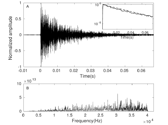
The envelope of the multi-reverberated impulse response shows exponential decay. By fitting an exponential function to the squared signal (intensity), an attenuation time (time that it takes for the amplitude to decrease by 1/e of the maximum amplitude) of 9 ms is found. At 10 KHz, this time corresponds to about 18 reflections off the boundaries. For a single pair of receivers separated by 12 cm and placed at minimum distance of about 19 cm from the borders of the plate, the cross-correlations for all of the virtual noise source positions are gathered in Figure 3A, while Figure 3B shows the results of the averaging over all of the source positions. A coherent structure clearly appears in Figure 3A that appears to be symmetric in time. This is confirmed in Figure 3B and 3C, which are remarkably symmetric, including several reverberated arrivals after the direct wave.

Figure 3: (A) Cross-correlation gather for all of the available virtual point sources (2,773 points) distributed uniformly on the plate. (B) Comparison of the normalized cross-correlation averaged over all of the source positions (black), and direct measurement of the source-to-receiver ”time-integrated” impulse response (gray). (C) Comparison between the positive time (black) and the (flipped) negative time (gray) contributions of the averaged cross-correlations. All of the cross-correlations in this plot are bandpass filtered by a Butterworth filter of 4th order between 15 KHz and 30 KHz, and normalization is performed with respect to the maximum energy of the correlated signals.

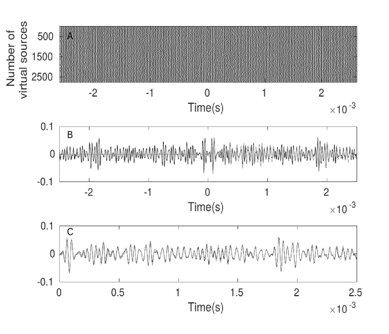
As transducers are reciprocal devices, they can also be efficiently used as emitters. What we measure is the convolution of the electro-elastic response of the transducer that acts as the source, the Green’s function, the electro-elastic response of the transducer that acts as the reciever, and the emitted signal. Note that this $G(t)$ is the vertical-vertical component of the Green’s function. We assume that within the frequency band of interest, the frequency responses of the transducers are flat, and hence the impulse response is obtained by applying pulse compression of the emitted signals on the recordings. Hence, the impulse response can be measured directly between the pair of transducers. The time-integration result of this directly measured response after pulse compression ($G(t)$) of the emitted signal is compared with the cross-correlation, to validate the theoretical result (Eq. (3)), as discussed in section II. There is excellent agreement between the two, even for multiply reflected contributions, as shown in Figure 3B (similar to the results of Mikesell2012 ). This impulse response corresponds to the vertical component of the Green’s function. See Supplemental Material (part IV) at [URL] for the location of the transducers on the plate (supple ).

IV Symmetry of the cross-correlation of the observed data

We infer from Figure 3 that to a good approximation, the cross-correlation is symmetric with respect to time when averaged over all of the available sources in the two-dimensional plate. Its symmetry in time is often used as a signature of its convergence toward the Green’s function (e.g., Roux2005 ). In this section, we quantitatively study the dependence of the time symmetry of the cross-correlation on the number of sources.
To this end, $C_{N}(t)$ (i.e., the cross-correlation averaged over $N$ sources) can be written as the sum of two terms:

$$C_{N}(t)=C_{N}^{+}(t)+C_{N}^{-}(t),$$ (4)

where

$$C_{N}^{+}(t)=\frac{C_{N}(t)+C_{N}(-t)}{2}\textrm{ and }C_{N}^{-}(t)=\frac{C_{N}(t)-C_{N}(-t)}{2},$$ (5)

where for the sake of simplicity, $\textbf{r}_{l}^{R}$ and $\textbf{r}_{l^{\prime}}^{R}$ have been dropped from the argument of $C_{N}$.

By definition, $C_{N}^{+}(t)$ (resp. $C_{N}^{-}(t)$) is symmetric (resp. antisymmetric) with respect to time.

We then compute the ratio of the integrated squared $C_{N}^{+}(t)$ and $C_{N}^{-}(t)$; i.e.,

$$r_{N}\triangleq\frac{\int_{-\infty}^{+\infty}C_{N}^{+}(t)^{2}dt}{\int_{-\infty}^{+\infty}C_{N}^{-}(t)^{2}dt}.$$ (6)

In Figure 4, the experimental estimation of this symmetry ratio is plotted with respect to the number of sources used in the averaging process. This curve is determined by repeatedly implementing Equation (6), based on a growing number of randomly distributed sources, until all of the available sources are taken into account.

Figure 4: $r_{N}$ as a function of the number of sources $N$ picked randomly, derived from the experimental data (blue star line) using Equation (6), and modeled (dashed red line) based on the theory developed in section IV and summarized by Equation (14). A 4th order Butterworth filter between 5000 Hz and 15000 Hz is applied to experimental data.

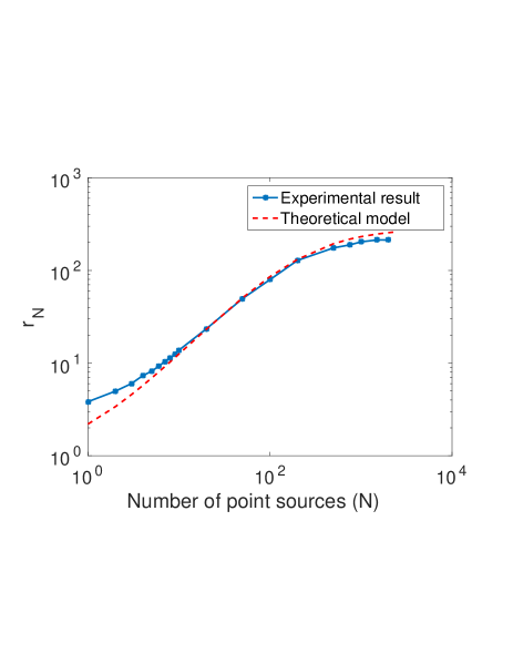
From Figure 4, it appears that the cross-correlation is far from symmetric if only a limited number of sources are used in the averaging process. In this case, the assumptions that allowed the derivation of Equation (3) do not hold. Nevertheless, as the number of sources grows, the averaged cross-correlation becomes more and more symmetric in time. This behavior is directly related to the convergence of the Green’s function reconstruction. Let us first write the cross-correlation obtained for a subset $N$ of all of the point sources as

$$C_{N}(t)=C_{\infty}(t)+\delta C_{N}(t),$$ (7)

where $C_{\infty}(t)$ is the cross-correlation obtained when all of the recordings from all of the available sources in this experimental set-up are taken into account.

While $C_{\infty}(t)$ is the best possible approximation of the Green’s function, given the experimental set-up, there is no such thing as a perfectly uniform source distribution and infinite source density in practical applications. It follows that $C_{\infty}(t)$ does not exactly coincide with $ImG$ (see Eq. (3)), and should in principle be slightly asymmetric with respect to time. After defining the symmetric and antisymmetric components of $C_{\infty}(t)$, similar to Equation (5), and substituting Equation (7) into Equation (5) and Equation (6), we find that

$$r_{N}=\frac{4\int_{-\infty}^{+\infty}C_{\infty}^{2}(t)dt+2\int_{-\infty}^{+\infty}\delta C_{N}^{2}(t)dt}{4\int_{-\infty}^{+\infty}(C_{\infty}^{-}(t))^{2}dt+2\int_{-\infty}^{+\infty}\delta C_{N}^{2}(t)dt},$$ (8)

where $C_{\infty}^{-}(t)$ is the antisymmetric component of $C_{\infty}(t)$. Equation (8) is directly related to the ratio of the noise level (L), which is a measure of the quality of the reconstructed Green’s function from a finite number $N$ of sources compared to the one obtained over an infinite number of sources introduced in Moulin2015 . This can be expressed in terms of $C_{\infty}(t)$ and $\delta C_{N}(t)$

$$L=\frac{\int_{-\infty}^{+\infty}\delta C_{N}^{2}(t)dt}{\int_{-\infty}^{+\infty}C_{\infty}^{2}(t)dt}.$$ (9)

Thus, Equation (8) can now be rewritten as

$$r_{N}=\frac{2+L}{2\zeta+L}$$ (10)

where $\zeta=\int(C_{\infty}^{-}(t))^{2}dt/\int C_{\infty}^{2}(t)dt$ is the relative degree of asymmetry of the cross-correlation function when $N\rightarrow\infty$. For a rectangular plate, L is given by Moulin2015

$$L\approx\frac{\pi n_{0}}{N\tau_{a}},$$ (11)

where $\tau_{a}$ is the attenuation time and $n_{0}$ is the plate modal density (modes per unit of frequency $\omega$), which in turn depends on the area of the plate surface $A$, the surface density $\rho_{s}$, and the bending stiffness $D$, through the relationshipFahy2007

$$n_{0}=\frac{A}{4\pi}\sqrt{\frac{\rho_{s}}{D}}.$$ (12)

Then, defining $k$ as the ratio of the attenuation time to the modal density,

$$k=\frac{\tau_{a}}{n_{0}},$$ (13)

Equation (10) finally becomes

$$r_{N}=\frac{1+2Nk/\pi}{1+2\zeta Nk/\pi}$$ (14)

By finding adequate values of $k$ and $\zeta$, the best-fit is obtained at 1.9 and 0.0035, respectively, which results in the dashed red curve in Figure 4. On the other hand, the experimental values for $\tau_{a}$ and $n_{0}$ are 0.009 s and 0.005 s/rad, respectively, which leads to $k=1.8$, according to Equation 13. This experimental value for $k$ and that obtained from the fitting are consistent. The relative degree of asymmetry $\zeta$ can be explained as a consequence of the fact that the laser vibrometer is only sensitive to vertical displacement (mainly $A_{0}$ mode). However, to some extent, the transducer also excites in-plane components (mainly $S_{0}$ and $SH$ mode). As a result, the in-plane components modes do not contribute to the reconstruction of the Green’s function.

V Similarity between impulse response and cross-correlation

The Pearson similarity coefficient between the two signals $G(t)$ and $C_{N}(t)$ is defined as (e.g., Press1992 ),

$$S({G,C_{N}})=\frac{\left\langle\left|\int_{\Delta\theta}G(t)C_{N}(t)dt\right|\right\rangle}{\sqrt{\left\langle\int_{\Delta\theta}G(t)^{2}dt\right\rangle\left\langle\int_{\Delta\theta}C_{N}(t)^{2}dt\right\rangle}},$$ (15)

where $\Delta\theta$ is the time-integration window to compute the similarity coefficient, and $\langle\ldots\rangle$ is the averaging over the different sets of point sources that are picked randomly. The latter is required for $S({G,C_{N}})$ to be independent of the measurement positions. While the word ’similarity’ is preferred here for clarity, $S$ is more often referred to in the literature as the ’correlation’ coefficient Press1992 . Figure  5 shows $S({G,C_{N}})$; i.e., the similarity coefficient between the time-integrated impulse response and the cross-correlation of signals recorded at transducers #3 and #4 for increasing number of sources. The similarity coefficient $S({G,C_{N}})$ is computed over a time window with a length ($\Delta\theta$) equal to the decay time $\tau_{a}$ (see Fig. 5).

Figure 5: Similarity coefficient $S({G,C_{N}})$ between the $C_{N}(t)$ and $G(t)$ versus the number of point sources (picked randomly) when the whole time signal is cross-correlated (solid line), and when only a part of the coda signal ($dT=0.2$ s; see Eq. 16) is cross-correlated (dashed line). A 4th order Butterworth filter between 15 KHz and 30 KHz is applied on $C_{N}(t)$ and $G(t)$. $\Delta\theta$ is equal to the attenuation time. Curve with the star symbols is $S({G,C_{N}})$ where $C_{N}(t)$ is the result of the averaged cross-correlation of only direct-arrival window. In this case, $\Delta\theta$ is 0.7 ms.

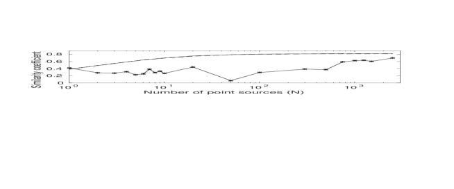
To discriminate the contribution of the direct arrival, we have also plotted $S({G,C_{N}})$ where only direct arrivals are cross-correlated to get $C_{N}$. We clearly observe a lower similarity unless there exists a very large number of sources. However, this contribution is negligible because when we cross-correlate the coda i.e., all the reverberated signal without direct arrival, the same value of the similarity coefficient is obtained as when all the signal is cross-correlated.
First, for a large number of sources ($N>100$), $S({G,C_{N}})$ reaches a plateau ($s\approx 0.82$) that is less than 1.0. From the analysis of the symmetry of the correlation, we measured that the latter is asymmetric with $\zeta=0.0035$. Assuming that the deviation to the perfectly reconstructed Green’s function is as much symmetric as anti-symmetric, the total deviation reaches 0.0070. Consequently, the difference with the 18% mismatch observed in Fig.  5 cannot be explained by the missing of in-plane components to the reconstructed Green’s functions. We interpret this increase of discrepancy by the fact that when considering the directly measured Green’s function, the effect of the transducer response appears as the convolution of the two transducer responses, while when the recordings are cross-correlated, we deal with the cross-correlation of the transducer responses. A probably weaker effect comes from the absorption by the transducers that induces a deviation from the Green’s function estimation as shown in Davy2016 .

Secondly, somewhat surprisingly, even with only one or very few sources the cross-correlation matches the time-integrated Green’s function relatively well ($S\approx 0.4$), even when only a part of the coda is correlated.

In the next two sections, we propose models to explain these behaviors. This begins with a study of the impact of the number of noise sources and the length of the correlated coda on the emergence of the Green’s function. Then, the effects of uncorrelated noise are taken into account.

VI Correlation of windowed coda

We next study the contribution of different parts of the coda signal to the reconstruction of the Green’s function. In practice, rather than cross-correlating the entire signal, as above, the cross correlation is now limited to a time interval of variable length, where the variable start-point and end-point are denoted as $T_{0}$ and $T_{0}+dT$, respectively. This is expressed by

$$C_{N}^{dT}(\textbf{r}_{l}^{R},\textbf{r}_{l^{\prime}}^{R},t)=\sum_{k=1}^{N}\int_{T_{0}}^{T_{0}+dT}{G(\textbf{r}_{l}^{R},\textbf{r}_{k}^{S},\tau)G(\textbf{r}_{l^{\prime}}^{R},\textbf{r}_{k}^{S},\tau-t)d\tau}.$$ (16)

Note that there is a distinction between the two time windows $dT$ and $\Delta\theta$ defined in Equation (15); the former is the cross-correlation window, while the latter is the time window over which the similarity coefficient is computed.

Figure 6: Comparison of the cross-correlation results for three different time windows when the sources are distributed over all of the plate, considering the whole length of the signal (black line), only the ballistic part of the signal [$dT$ = 0.7 ms] (blue dots), and only a part of the coda arrivals [$T_{0}$ = 0.4 ms, $dT$ = 0.02 s] (gray dashed line). All the cross-correlations are bandpass filtered between 15 KHz and 30 KHz by a 4th order Butterworth filter.

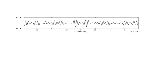
In Figure 6, cross-correlations are compared when the time window includes: only the ballistic wavefront, only the multi-reverberated waves, and the whole wavefield. We observe that cross-correlation of only the ballistic part of the signals builds only the ballistic part of the Green’s function, while cross-correlation of the coda part reconstructs both the ballistic and coda parts of the Green’s function. Moreover, the contribution due to the ballistic path is negligible, and the recovery of the Green’s function is dominated by the coda part.

To study the convergence process, the similarity coefficient is computed between a reference cross-correlation $C_{ref}(\textbf{r}_{l}^{R},\textbf{r}_{l^{\prime}}^{R},t)$ and the cross-correlation function obtained for different time windows, averaged over randomly-picked sources $C_{N}^{dT}(\textbf{r}_{l}^{R},\textbf{r}_{l^{\prime}}^{R},t)$. We recall that $C_{ref}(\textbf{r}_{l}^{R},\textbf{r}_{l^{\prime}}^{R},t)$ is obtained when all of the sources are emitting and all of the signals are cross-correlated. In this section and the next one, the reference to obtain the similarity coefficient is not the empirical Green’s function ($G(t)$), but $C_{ref}(\textbf{r}_{l}^{R},\textbf{r}_{l^{\prime}}^{R},t)$. The reason for this is that according to Figure 5, $G(t)$ never perfectly converges to $C_{ref}(\textbf{r}_{l}^{R},\textbf{r}_{l^{\prime}}^{R},t)$, and they are not perfectly similar, which avoids reaching 1.0 for the similarity coefficient even when all of the sources are considered and the cross-correlation is over the whole signal. Also, as explained before, this new choice for reference circumvents any influence on the results by the difference in the frequency response of the transducers and the vibrometer.

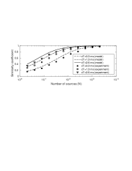
The similarity coefficient $S({C_{ref},C_{N}^{dT}})$ is computed in a window that contains the direct arrivals and that lasts as long as the attenuation time, following Equation 15. Figure 7 shows the values of $S({C_{ref},C_{N}^{dT}})$ versus the number of point sources ($N$) for the three different correlation window lengths ($dT$). It can be seen that all of the curves have a similar trend. The values of the similarity coefficient ($S({C_{ref},C_{N}^{dT}})$) increase with the number of sources ($N$), and the resulting cross-correlation converges toward the reference one after a certain number of sources, which indicates that the cross-correlation of a short time window (compared to the decay time $\tau_{a}$ = 9 ms) leads to a reasonable impulse response.

Figure 7: Similarity coefficient $S({C_{\infty},C_{N}^{dT}})$ between $C_{\infty}$ and $C_{N}^{dT}$ (cross-correlation obtained by windowing one signal before the cross-correlation, and then averaged over a subset of available sources picked at random). Symbols and lines show the experimental results and theoretical model, respectively, for the various window lengths ($dT)$. The starting time ($T_{0}$) in all three cases is 2.3 ms, i.e., no ballistic signal is cross-correlated.

See Supplemental Material (part I) at [URL] for our proposed model based on the modal decomposition of the plate Green’s function solution of Equation (1) to derive $S{({C_{ref},C_{N}^{dT}})}$ (supple ). Note that in the theoretical approach, we refer to the reference cross-correlation or the “perfect” cross-correction by ${C_{\infty}}$. This difference in the notation between the theoretical $({C_{\infty}})$ and experimental $({C_{ref}})$ approach is a reminder for the fact that in the experimental case we cannot have an infinite number of sources and hence a perfect cross-correlation. $S({C_{\infty},C_{N}^{dT}})$ is finally given by

$$S({C_{\infty},C_{N}^{dT}})=\left[1+\frac{2}{N}\left(1+Z\right)\right]^{-0.5},$$ (17)

with

$$Z=\frac{\int\kappa(\delta\omega,\omega){\left|\widetilde{M}(\delta\omega)\right|^{2}}d\delta\omega}{\left|\widetilde{M}(0)\right|^{2}\left(1+F(\delta r)\right)},$$ (18)

where $F(\mathbf{\delta}r)$ accounts for the spatial correlation of the squared eigen-modes, $N$ is the number of point sources, $\kappa(\delta\omega,\omega)$ is the two-level correlation and $\tilde{M}$ is the Fourier transform of the time windowed (the window duration being $dT$) squared mean intensity (see Supplemental Material for more details (supple )).

The two-level correlation function, that has been formally introduced in quantum chaos theory, is defined in terms of the modal density ($n_{0}(\omega)$) as

$$\kappa(\delta\omega,\omega)=\frac{\left\langle n_{0}(\omega)n_{0}(\omega+\delta\omega)\right\rangle}{\left\langle n_{0}(\omega)\right\rangle}.$$ (19)

LyonLyon1969 also introduced it when analyzing the statistical properties of sound power in structures.

In a chaotic-shaped plate, due to repulsion between the modes, $\kappa$ is null when $\delta\omega=0$ and is close to $n_{0}$ when $\delta\omega$ is larger than the modal density. The expression of $\kappa$ can be found in Mehta2004 ; Wright2010 . But here, as the plate geometry is regular, the eigen-frequency statistics follow a Poisson’s distributionLyon1969 ; Efetov1983 . As a consequence, there are no correlations between the eigenfrequencies, $\kappa(\delta\omega,\omega)$ is equal to the modal density and Z can be simplified into

$$Z=\frac{\pi n_{0}}{\tau_{a}\left(1+F(\delta r)\right)}\mathrm{coth}\left(\frac{dT}{\tau_{a}}\right).$$ (20)

The coefficient $Z$ can be interpreted as the average number of overlapping modes of the plate within the windowed cross-correlation at angular frequency $\omega$.

See Supplemental Material (part III) at [URL] on derivation of the expressions for the spatial correlation of the squared eigenmodes and $F$ for chaotic and rectangular cavities (supple ). In the case of a chaotic cavity, based on the Berry conjectureBerry1977 , $F(\mathbf{\delta}r)$ is given by $2J_{0}(k\delta r)^{2}$, where $J_{0}$ is the zero-th order Bessel function of the first kind. In the case of a rectangular cavity, using the same methodology as the one that led to the spatial correlation of the eigenmodes in a rectangular plateBonilha1998 , we find

$$F(\mathbf{\delta}r)=\frac{J_{0}(2k\left|\delta x\right|)+J_{0}(2k\left|\delta y\right|)}{2}+\frac{J_{0}(2k\delta r)}{4}.$$ (21)

Note that now the correlation of squared eigenmodes is anisotropic because it not only depends on modulus of $\delta\mathbf{r}$, but also on the projection $dx$ (respect. dy) of $\delta\mathbf{r}$ along the x-axis (respect. y-axis).

The continuous curves in Figure 7 result from the model described by Equation (17), where $F(\delta r)\sim 1/2$ for $\delta r\gg\lambda$ and $1+F(\delta r)$ is set to 1.5. We believe that this long-range correlation is due to strong periodic orbits that are not taken into account by our correlation models.

The convergence toward the Green’s function is driven by three characteristic times: the modal density ($n_{0}$), the attenuation time of the plate ($\tau_{a}$); and the time window selected for the cross-correlation ($dT).$ Schematically, three asymptotic cases can be identified:

1. When $\tau_{a}\gg n_{0}$ and $dT\gg n_{0}$, the modes of the plate are resolved because the attenuation is low (see Fig.  8a). Moreover, the integration time $dT$ is sufficiently large to include a sufficient amount of coda to not induce modal overlapping by a windowing effect. In such a case, the similarity coefficient $S({C_{\infty},C_{N}^{dT}})$ is high, and therefore the ’best’ correlation is obtained. In the case of a single source $S({C_{\infty},C_{N}^{dT}})$ is $1/\sqrt{3}$.

2. When $\tau_{a}\lesssim n_{0}$ and $dT\gg\tau_{a}$, $Z\approx\pi n_{0}/\tau_{a}$, the overlapping due to the attenuation is not negligible anymore (see Fig.  8b). The convergence of the cross-correlation toward the Green’s function is slower. Hence, at least Z sources are required to obtain a good estimation of the Green’s function from the cross-correlation.

3. Finally when, $dT\ll\tau_{a}$ and $dT\lesssim n_{0}$, the mode overlapping is dominated by the effects of the coda truncation, and is given by $Z\approx\pi n_{0}/dT$ (see Fig.  8c). Again, to get a good estimation of the Green’s function, at least Z sources have to be used.

Hence, when $N$ is large compared to $1+Z$, $S({C_{\infty},C_{N}^{dT}})$ converges toward 1.0, independent of the window length $dT$. In other words, even with a very short integration time in Equation (16), the Green’s function can be completely recovered.

Figure 8: Three schematic representations of a small part of the Fourier transform of the window cross-correlations for different values of the characteristic times of the system, namely as: modal density ($n_{0}$), attenuation time ($\tau_{a}$), and selected time window for cross-correlation ($dT$). The vertical arrows mark the eigen-modes that are separated on average by $\frac{1}{n_{0}}$. The dashed curves represent Lorentzian spectra of the width $1/\tau_{a}$, which is the inverse Fourier transform of the exponential attenuation. Finally, the dotted curves show the sinc functions of the width 1/dT, which is the Fourier transform of the window. The regimes and the corresponding approximate values of $Z$ are denoted at the top righthand corner of each plot.

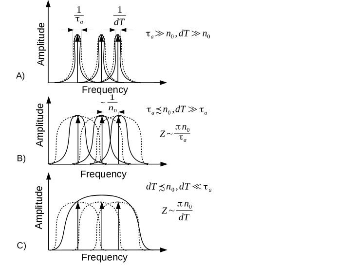
Figure 7 shows that the experimental results approximately confirm this model; the similarity coefficient $S({C_{\infty},C_{N}^{dT}})$ does not converge to 1.0 exactly, which we ascribe to the presence of a small amount of random noise in the measurements.

VII Effects of random noise

A comparison between the model and the experimental results (Fig. 7) suggests that uncorrelated noise (e.g., electronic noise) degrades the Green’s function. We next analyze this effect by performing the cross-correlation over time windows that start between $T_{0}=0$ and $T_{0}=57$ ms after the beginning of the transient response, and end at time $T_{0}+dT=250$ ms (see inset in Fig. 9). Time $T_{0}+dT$ is chosen to be a lot larger than $\tau_{a}$, to increase the relative contribution of noise in the correlation process. The similarity coefficient $S({C_{ref},C_{ref}^{dT}})$ is then retrieved according to Equation 15 and from the direct path and primary coda signal ($\Delta\theta=2$ ms). As for the previous section, the reference of the similarity coefficient is the one obtained when the number of sources is large and the effects of noise are negligible. Note that, in this case, all of the sources $N$ are considered in the computation of $S({C_{ref},C_{ref}^{dT}})$, and the similarity coefficient is plotted in Figure 9 as a function of $T_{0}$.

Figure 9: $S({C_{\infty},C_{\infty}^{dT}})$ between $C_{\infty}(\textbf{r}_{l}^{R},\textbf{r}_{l^{\prime}}^{R},t)$ and $C_{\infty}^{dT}(\textbf{r}_{l}^{R},\textbf{r}_{l^{\prime}}^{R},t)$ given by Equation (16). The end of the time windows ($T_{0}+dT)$ is fixed at 250 ms. $S({C_{\infty},C_{\infty}^{dT}})$ is then evaluated in a window that includes direct path and primary coda ($\Delta\theta=2$ ms).

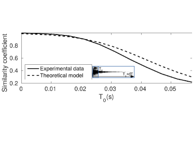
We observe that the effects of noise becomes significant only when $T_{0}$ is $>$15 ms. The decay of the $S({C_{ref},C_{ref}^{dT}})$ can be explained by assuming that the field measurement is perturbed by a constant amount of uncorrelated noise at each transducer, according to Equation (22). See Supplemental Material (part II) at [URL] for the complete derivation of $S({C_{\infty},C_{\infty}^{dT}})$ (supple ). Similar to the previous section, we discriminate the experimental case from the theoretical one by changing ${C_{ref}}$ to ${C_{\infty}}$. After some algebra, we find

$$S({C_{\infty},C_{\infty}^{dT}})\approx\left(1+\frac{\beta B(dT)}{N[e^{-T_{0}/\tau_{a}}(1-e^{-dT/\tau_{a}})]}\right)^{-0.5},$$ (22)

where $B$ is the bandwidth of the system, and the dimensionless value $\beta$ is an indication of the noise-to-signal ratio.

The experimental data were fitted to Equation (22). We observe that the model explains the decay in $S({C_{ref},C_{ref}^{dT}})$ and as we go further in time, it is the noise content that dominates, which consequently causes degradation of the reconstructed Green’s function. Note that unlike the experimental curve, the theoretical one does not start from the value of 1.0. This is due to a different reference in the similarity coefficient in these two cases. On the one hand, for $T_{0}=0$, the correlation and the reference correlation are identical because we chose the best correlation possible for the reference cross-correlation (i.e., at $T_{0}=0$). Consequently, $S({C_{ref},C_{ref}^{dT}})$ is exactly 1.0. On the other hand, from a theoretical point of view $S({C_{\infty},C_{\infty}^{dT}})$ is smaller than 1.0 because the reference correlation is the ideal one, i.e., the difference between the advanced and delayed Green’s function, while the noise slightly contaminates the cross-correlation.

VIII Discussion

As explained by Derodeandlarose , the process of reconstructing a Green’s function by diffuse-field cross-correlation is closely related to that of acoustic time reversal Derode2003 . Accordingly, this study has some implications in the context of time reversal. To illustrate this point, let us assume that a pulse is sent at position $\textbf{r}_{A}$ and the $N$ transient responses are recorded by $N$ receivers at positions $\textbf{r}_{i}$. Each response is then flipped in time and sent back into the medium by the $N$ emitters located at the same positions as the $N$ receivers. In a reciprocal medium, it can be formally shown that the time-dependent amplitude of the time-reversed field at position $\textbf{r}_{B}$ is proportional to the correlation $C_{N}(t)$ between positions $\textbf{r}_{A}$ and $\textbf{r}_{B}$. When only a part of the transient responses between times $T_{0}$ and $T_{0}+dT$ are flipped and sent back, the time-reversed field is then given by $C_{N}^{dT}(t)$. This formal equivalence between the cross-correlation and the time reversal provides new insights Derode2003 . First, when there is only one source, the cross-correlation behaves approximately as the one-channel time-reversal signal of flexural waves obtained by Draeger and Fink Draeger1997 . In particular, it has been shown that in a lossless cavity, the time reversed field at position $\mathbf{r}_{1}$ is equal to $G(\mathbf{r}_{1},\mathbf{r}_{1},t)\otimes G(\mathbf{r}_{A},\mathbf{r}_{B},-t)$ Draeger1999 . For this set-up, we infer from Equations (17) and (20) that when $dT\gg\tau_{a}\gg n_{0}$, the similarity coefficient $S(C_{\infty},C_{1}^{dT})$ for one single source is equal to $1/\sqrt{3}$. Hence, the mismatch is due to $G(\mathbf{r}_{1},\mathbf{r}_{1},t)$, i.e., fluctuations induced by alternation of nodes and antinodes at $\mathbf{r}_{1}$. Secondly, the case where the sources are uniformly distributed over the surface corresponds to the instantaneous time reversal, which is also called the Loschmidt echo Loschmidt1876 . In this case, a field can be perfectly time reversed at time $t_{0}$ by imposing the initial condition $\psi(\mathbf{r},t_{0})$ and its negative time derivative $-\partial\psi(\mathbf{r},t_{0})/\partial t$. Consequently, by time reversing a very small window around time $t_{0}$ of the transient responses by many sources over all of the surface, the time-reversed field is perfectly recovered for $t<t_{0}$. This result is in agreement with our finding that $S(C_{\infty},C_{N>>1}^{dT})$ converges to 1.0 as $N$ grows.

A popular technique used in order to improve the estimation of the Green’s function consists of correcting the exponential attenuation decay to artifically increase the attenuation time. In such a case, because $\tau_{a}$ is larger (see Eq. (14)), the symmetry ratio $r_{N}$ increases faster with the number of sources. The similarity coefficient is also improved because $\tau_{a}$ can be larger than the modal density (also called Heisenberg time) and the system behaves as if the plate modes are resolved (see Eq. (17)). However, this correction also increases exponentially noise-to-signal ($\beta$) and therefore limits the efficiency of the method (see Eq. (22)).

In the case of continuous incoherent noise sources, the cross-correlation converges toward the windowed cross-correlation, but with a window that includes all of the transient signal. The present study provides new insights into the understanding of the relative contributions of the different parts of the transient response (e.g., ballistic and early coda, late coda) for building the cross-correlation. Considering the transient recorded signals that consist of direct and later arrivals, and cross-correlating these parts of the signals separately, we show that exclusion of the direct arrivals and cross-correlation of only the coda arrivals is very close to the case where we cross-correlate the full-time signals.

IX Conclusions

Given any receiver pair, the signal that would be obtained at either one from a source at the other can be reconstructed experimentally by cross-correlation of the recordings of a diffuse field. The field can be diffuse as a result of a dense, homogeneous source distribution throughout the medium, and/or of scattering or reverberation: this study was aimed at the disentangling of these two effects. We conducted experiments with a thin plate where the surface was densely scanned by a laser vibrometer, and where an array of transducers was deployed. This set-up provides almost perfect control of the spatial distribution of the transient sources. We first validated the theory through comparison of the averaged cross-correlations and the directly observed Green’s function. We also experimentally studied the symmetry (with respect to time) of the cross-correlations, as well as their similarity to the Green’s function, as a function of the number of uniformly distributed point sources. To explain these observations quantitatively, a theoretical analytical model was developed that predicts the observed asymmetry of the averaged cross-correlation. We next studied the convergence of the averaged cross-correlation for time windows of variable lengths, which might be very short, and taken at different points in the coda of the recordings. Here, a relatively dense/ uniform source distribution can result in good estimation of the Green’s function. We demonstrated that this time window does not have to include the direct-arrival part of the signals for the estimated Green’s function to be a good approximation of the exact one. Through statistical modal analysis, the respective contributions of attenuation time, modal density, and number of sources to the convergence of the cross-correlation toward the Green’s function were identified. Finally, we demonstrated both theoretically and experimentally that this convergence strongly depends on the position of the correlation time window only when additive random noise is taken into account. The relative effects of the noise are stronger when the late coda is cross-correlated.

References

- [1] R.L. Weaver and Oleg I. Lobkis. Ultrasonics without a source: Thermal fluctuation correlations at mhz frequencies. Physical Review Letters, 87(13), 2001.
- [2] R. Snieder, A. Gret, H. Douma, and J. Scales. Coda wave interferometry for estimating nonlinear behavior in seismic velocity. Science, 295:2253–2255, 2002.
- [3] M. Campillo and A. Paul. Long-range correlations in the diffuse seismic coda. Science, 299(5606):547–549, 2003.
- [4] OI. Lobkis and RL Weaver. On the emergence of the green’s function in the correlations of a diffuse field. Journal of the Acoustical Society of America, 110(6):3011–3017, December 2001.
- [5] J. Rickett and J. Claerbout. Acoustic daylight imaging via spectral factorization: helioseismology and reservoir monitoring. Leading Edge, 18:957–960, 1999.
- [6] P. Roux, W. A. Kuperman, and NAPL Grp. Extracting coherent wave fronts from acoustic ambient noise in the ocean. J. Acoust. Soc. Am., 116(4, Part 1):1995–2003, October 2004.
- [7] M. Campillo, P. Roux, B. Romanowicz, and A. Dziewonski. Seismic imaging and monitoring with ambient noise correlations. Treatise on Geophysics, pages 256–271, 2014.
- [8] L. Boschi and C. Weemstra. Stationary-phase integrals in the crosscorrelation of ambient noise. Reviews of Geophysics, 2015.
- [9] K. Sabra, S. Conti, P. Roux, and W. Kuperman. Passive in vivo elastography from skeletal muscle noise. Appl. Phys. Lett., 90, 2007.
- [10] K.G. Sabra, A. Srivastava, F.L. di Scalea, I. Bartoli, P. Rizzo, and S. Conti. Structural health monitoring by extraction of coherent guided waves from diffuse fields. The Journal of the Acoustical Society of America, 123(1):EL8–EL13, 2008.
- [11] K. Wapenaar, J. Fokkema, and R. Snieder. Retrieving the green’s function in an open system by cross correlation: A comparison of approaches (l). The Journal of the Acoustical Society of America, 118(5):2783–2786, 2005.
- [12] Richard L. Weaver and Oleg I. Lobkis. Diffuse fields in open systems and the emergence of the green’s function (l). J. Acoust. Soc. Am., 116:2731, 2004.
- [13] P. Roux, K. Sabra, W. A. Kuperman, and A. Roux. Ambient noise cross correlation in free space: Theoretical approach. J. Acoust. Soc. Am., 117(1):79–84, 2005.
- [14] E. Larose, P. Roux, M. Campillo, and A. Derode. Fluctuations of correlations and green’s function reconstruction: role of scattering. Journal of Applied Physics, 103(11):114907, 2008.
- [15] B. A. van Tiggelen. Green function retrieval and time reversal in a disordered world. Phys. Rev. Lett., 91(24):243904, DEC 12 2003.
- [16] J. de Rosny and M. Davy. Green’s function retrieval and fluctuations of cross density of states in multiple-scattering media. EPL (Europhysics Letters), 106(5):54004, 2014.
- [17] T. Nowakowski, L. Daudet, and J. de Rosny. Localization of acoustic sensors from passive green’s function estimation. The Journal of the Acoustical Society of America, 138(5):3010–3018, 2015.
- [18] L. Chehami, J. de Rosny, C. Prada, E. Moulin, and J. Assaad. Experimental study of passive defect localization in plates using ambient noise. IEEE transactions on ultrasonics, ferroelectrics, and frequency control, 62(8):1544–1553, 2015.
- [19] E. Larose, P. Roux, and M. Campillo. Reconstruction of rayleigh–lamb dispersion spectrum based on noise obtained from an air-jet forcing. The Journal of the Acoustical Society of America, 122(6):3437–3444, 2007.
- [20] A. Colombi, L. Boschi, P. Roux, and M. Campillo. Green’s function retrieval through cross-correlations in a two-dimensional complex reverberating medium. The Journal of the Acoustical Society of America, 135(3):1034–1043, 2014.
- [21] A. Duroux, K.G. Sabra, J. Ayers, and M. Ruzzene. Extracting guided waves from cross-correlations of elastic diffuse fields: Applications to remote structural health monitoring. The Journal of the Acoustical Society of America, 127(1):204–215, 2010.
- [22] L.E. Kinsler, A.R. Frey, A.B. Coppens, and J.V. Sanders. Fundamentals of Acoustics. Wiley, Hoboken, N.J., 1999.
- [23] D. Royer and E. Dieulesaint. Elastic waves in solids I. Springer-Verlag Berlin, Heidelberg, 2000.
- [24] E. Ventsel and T. Krauthammer. Thin plates and shells : theory : analysis, and applications. Marcel Dekker, Inc., 2001.
- [25] F. Fahy and P. Gardonio. Sound and structural vibration, radiation, transmission and response. Academic Press, 2007.
- [26] L. Chehami, E. Moulin, J. de Rosny, C. Prada, O. Matar, F. Benmeddour, and J. Assaad. Detection and localization of a defect in a reverberant plate using acoustic field correlation. Journal of Applied Physics, 115(10):104901, 2014.
- [27] K. Aki and P. G. Richards. Quantitative Seismology: Theory and Methods, Volumes I and II. W. H. Freeman & Co, 1980.
- [28] T. D. Mikesell, K. van Wijk, T. E. Blum, R. Snieder, and H. Sato. Analyzing the coda from correlating scattered surface waves. J. Acoust. Soc. Am., 131, 2012.
- [29] A. Hejazi Nooghabi, L. Boschi, P. Roux, and J. de Rosny. Supplemental material on similarity coefficient calculations between a reference cross-correlation and the cross-correlation obtained in two different cases: 1. time-limited cross-correlation. 2. instrumental noise affected recordings.
- [30] E. Moulin, F. Benmeddour, H. Achdijan, L. Chehami, J. Assaad, J. de Rosny, and C. Prada. Exploitation of the reverberant propagation of elastic waves in structures: towards a concept of low-resource shm sensor network. Physics Procedia, 2015.
- [31] W. H. Press, S. A. Teukolsky, W. T. Vetterling, and B. P. Flannery. Numerical recipes in c, the art of scientific computing. Cambridge University Press, 1992.
- [32] M. Davy, J. de Rosny, and P. Besnier. Green’s function retrieval with absorbing probes in reverberating cavities. Physical Review Letters, 116(21):213902, 2016.
- [33] RH Lyon. Statistical analysis of power injection and response in structures and rooms. The Journal of the Acoustical Society of America, 45(3):545–565, 1969.
- [34] Madan Lal Mehta. Random matrices, volume 142. Academic press, 2004.
- [35] Matthew Wright and Richard Weaver. New directions in linear acoustics and vibration: quantum chaos, random matrix theory and complexity. Cambridge University Press, 2010.
- [36] KB Efetov. Supersymmetry and theory of disordered metals. advances in Physics, 32(1):53–127, 1983.
- [37] M. Berry. Regular and irregular semiclassical wavefunctions. Journal of Physics A: Mathematical and General, 10(12):2083, 1977.
- [38] MW Bonilha and FJ Fahy. On the vibration field correlation of randomly excited flat plate structures, i: Theory. Journal of sound and vibration, 214(3):443–467, 1998.
- [39] A. Derode, E. Larose, M. Campillo, and M. Fink. How to estimate the green’s function of a heterogeneous medium between two passive sensors? application to acoustic waves. Appl. Phys. Lett., 83, 2003.
- [40] A. Derode, E. Larose, M. Tanter, J. de Rosny, A. Tourin, M. Campillo, and M. Fink. Recovering the green’s function from field-field correlations in an open scattering medium (l). The Journal of the Acoustical Society of America, 113(6):2973–2976, 2003.
- [41] C. Draeger and M. Fink. One-channel time reversal of elastic waves in a chaotic 2d-silicon cavity. Physical Review Letters, 79(3):407, 1997.
- [42] C. Draeger and M. Fink. One-channel time-reversal in chaotic cavities: Theoretical limits. The Journal of the Acoustical Society of America, 105(2):611–617, 1999.
- [43] J. Loschmidt. Uber den zustand des warmegleichgewichts eines systems von korpern mit rucksicht auf die schwerkraft. Sitzungsberichte der Akademie der Wissenschaften, 73:128–142, 1876.