Anti-Kibble-Zurek behavior of a noisy transverse-field XY chain and its quantum simulation with two-level systems
Abstract
We study the dynamics of a transverse-field XY chain driven across quantum critical points by noisy control fields. We characterize the defect density as a function of the quench time and the noise strength, and demonstrate that the defect productions for three quench protocols with different scaling exponents exhibit the anti-Kibble-Zurek behavior, whereby slower driving results in more defects. The protocols are quenching through the boundary line between paramagnetic and ferromagnetic phases, quenching across the isolated multicritical point and along the gapless line, respectively. We also show that the optimal quench time to minimize defects scales as a universal power law of the noise strength in all the three cases. Furthermore, by using quantum simulation of the quench dynamics in the spin system with well-designed Landau-Zener crossings in pseudo-momentum space, we propose an experimentally feasible scheme to test the predicted anti-Kibble-Zurek behavior of this noisy transverse-field XY chain with two-level systems under controllable fluctuations.
I introduction
Kibble-Zurek mechanism (KZM) provides an elegant theoretical framework for exploring the critical dynamics of phase transitions in systems ranging from cosmology to condensed matter Kibble1976 ; Zurek1985 ; Zurek1996 . The dynamics induced by a quench across a critical point with a control parameter is generally nonadiabatic due to the critical slowing down, which results in the production of topological defects. A key prediction of KZM is that the density of defects follows a universal power law as a function of the quench time (transition rate ): , where the scaling exponent determined by the critical exponents of the phase transition and the dimensionality of the system. KZM for classical continuous phase transitions has been verified in many systems, such as cold atomic gases Navon2015 , ion crystals Ulm2013 ; Pyka2013 , and superconductors Monaco2002 . There has been significant theoretical work on extension of KZM for quantum phase transitions Dziarmaga2010 ; Isingexact1 ; Isingexact2 ; Dziarmaga2006 ; Caneva2007 ; Xy1 ; XyMC ; Xy2 ; Deng2009 ; Sabbatini ; Kolodrubetz ; Caneva2008 ; Acevedo2014 , which are zero temperature transitions driven by Heisenberg quantum fluctuations rather than thermal fluctuations QPT . For instance, by studying KZM in the one-dimensional transverse-field Ising model, which is one of the paradigmatic models to study quantum phase transitions, it was found that the density of defects scales as the square root of the quench time with the scaling exponent Dziarmaga2010 ; Isingexact1 ; Isingexact2 . However, the experimental tests of KZM in quantum phase transitions are still scare since controlling the time evolution of systems cross quantum critical points is notoriously difficult Chen2011 ; Braun ; Anquez ; Chin .
Landau-Zener transition (LZT), occurring when a two-level system sweeps through its anticrossing point, has served over decades as a textbook paradigm of quantum dynamics of some non-equilibrium physics Landau ; Zener . Recently, LZT has been extensively studied Shevchenko both theoretically and experimentally in, e.g., superconducting qubits Oliver ; Sillanpaa ; Tan , solid-state spin systems Petta ; Betthausen ; Cao , and optical lattices Tarruell ; Salger ; Chen . It was shown that the dynamics of LZT can be intuitively described in terms of KZM of the topological defect formation in non-equilibrium quantum phase transition LZKZM1 ; LZKZM2 . The correspondence between the two physical situations provide a promising way for proof-of-concept quantum simulation of KZM in quantum regime by using LZT in two-level systems, which has been experimentally demonstrated in an optical interferometer Xu . Moreover, quantum simulation of the critical dynamics in the transverse-field Ising model by a set of independent Landau-Zener crossings in pseudo-momentum space has been realized in a semiconductor electron charge qubit LZKZMexp_QD , a superconducting qubit LZKZMexp_SC and a single trapped ion LZKZMexp_Ion . The LZT there can be engineered well and probed with high accuracy and thus KZM of defect production in the Ising model with the scaling exponent has been successfully observed in these artificial two-level systems LZKZMexp_QD ; LZKZMexp_SC ; LZKZMexp_Ion .
While KZM has been verified to be broadly applicable, a conflicting observation was reported in a recent experiment of ferroelectric phase transition: slower quenches generate more defects when approaching the adiabatic limit Griffin . This behavior is opposite to that predicted by the standard KZM and is termed as anti-Kibble-Zurek (anti-KZ) behavior. The quench dynamics of a transverse-field Ising chain coupled to a dissipative thermal bath has been theoretically studied in Refs. Santoro ; Nalbach , which show that the defect production can exhibit the anti-KZ behavior due to the emergence of thermal defects. Recently, by studying the crossing of the quantum critical point in a thermally isolated Ising chain driven by a noisy transverse field, it was demonstrated that noise contributions can also give rise to anti-KZ behavior when they dominate the dynamics Dutta . A natural question is whether the anti-KZ behavior can exhibit in other quantum spin models with different scaling exponents under noisy control fields. In the experimental aspect, it would be of great value to set a stage for quantum simulation of such anti-KZ behavior in two-level systems with Landau-Zener crossings, noting that quantum spin models can only be realized in some special situations without controllable noisy fields Kim ; Bohnet ; Simon , which may prevent the test of the anti-KZ behavior.
In this paper, we consider the dynamics of a transverse-field XY chain driven across quantum critical points by noisy control fields. We numerically calculate the defect density as a function of the quench time and the noise strength, and find that the defect productions in three quench protocols with different scaling exponents exhibit the anti-KZ behavior, i.e., slower driving results in more defects. The three protocols are quenching through the boundary line between paramagnetic and ferromagnetic phase, quenching across the isolated multicritical point and along the gapless line, which have the Kibble-Zurek scaling exponents under the noise-free driving Xy1 ; XyMC ; Xy2 , respectively. We also show that the optimal quench time to minimize defects scales as a universal power law of the noise strength in all three cases. Furthermore, by using quantum simulation of the quench dynamics in the spin system with well-designed Landau-Zener crossings, we then propose an experimentally feasible scheme to test the predicted anti-KZ behavior in this noisy transverse-field XY chain with two-level systems under controllable fluctuations in the control field. The driving protocols of the Landau-Zener crossings in two-level systems and the required parameter regions for observing the anti-KZ behavior in the three cases are presented.
The paper is organized as follows. In Section II, we illustrate that the defect productions of the transverse-field XY chain driven across quantum critical points by noisy control fields exhibit the anti-KZ behavior. In Section III, we propose to test the predicted anti-KZ behavior by using quantum simulation of the quench dynamics with well-designed LZT in two-level systems. Finally, a short conclusion is given in Sec. IV.
II Anti-KZ behavior of a noisy transverse-field XY chain
We begin with the spin- quantum XY chain under a uniform transverse field (homogeneous for each spin), which is one of the other exactly solvable spin models apart from the quantum Ising chain. The Hamiltonian of the transverse-field XY chain with nearest neighbor interaction is given by Lieb1961 ; Bunder1999
| (1) |
where (here and hereafter we set is even) counts the number of spins, () are the Pauli matrices acting on the -th spin, and respectively represent the anisotropy interactions along and spin directions, measures the strength of the transverse field. We set , , then the Hamiltonian can be rewritten as
| (2) | |||||
The system reduces to the isotropic XY chain for and the Ising chain for . This Hamiltonian can be exactly diagonalized by using the Jordan-Wigner transformation, which maps a system of spin-1/2 to a system of spinless free fermions Lieb1961 ; Bunder1999 ; Caneva2007 . The Jordan-Wigner transformation of spins to fermions is given by and , where . In the fermionic language, the XY model Hamiltonian can be rewritten as
| (3) | |||||
Under the periodic boundary condition with even requires that and after the Fourier transformation with , one can obtain , where and the Hamiltonian density in the pseodu-momentum space
| (4) |
Note that here and hereafter the Pauli matrices are conventionally used to write the Hamiltonian of each independent -mode ( pair), which is distinct from the spin components in Eqs. (1) and (2).
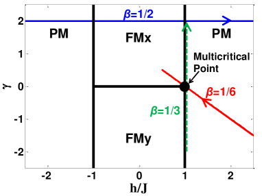
The energy spectrum of the system can be obtained by diagonalizing Eq. (4), and thus the critical points or lines between different quantum phases can be found by minimizing the energy gap. Figure 1 depicts the phase diagram of the transverse-field XY chain in the space spanned by the parameters and Xy1 . There are a quantum paramagnetic phase denoted by PM and two ferromagnetic long-ranged phases ordering along and directions denoted by FMx and FMy, respectively. As shown in Fig. 1, there are three kinds of phase phase boundaries: an Ising critical line on the horizontal axis (i.e. ), a multicritical point locates at , and two gapless lines along Xy1 ; XyMC ; Xy2 . Quantum phase transition occurs when the system is driven by one or more parameters to across the boundary line or point on the phase diagram.
To study the quench dynamics of the transverse-field XY chain, we can use the Hamiltonian decoupling into a sum of independent terms , where each -mode Hamiltonian given by Eq. (4) operates on a two-dimensional Hilbert space. The time evolution of a generic state is governed by the Schrödinger equation . This projection of the spin Hamiltonian to the Hilbert space has effectively reduced the quantum many-body problem to the problem of an array of decoupled two-level systems.
For the convenience of experimental implementation, we choose only one of the parameters and as linearly quenched in time and the rest fixed in a specific quench protocol. As shown in Fig. 1, we consider three different quench protocols for the system driven across the phase boundaries: (1) The transverse quench with only is varied in time, which is quenching through the boundary line between paramagnetic and ferromagnetic phase twice; (2) The anisotropic quench across the isolated multicritical point, in which case only the parameter is varying and is set to ensure passing through the multicritical point; (3) The quench along the gapless line, which requires that and only is varied. For the linear quench in the absence of dissipative thermal bath or noise fluctuations, the density of defects [see Eq. (11)] formed in three quench protocols follows the Kibble-Zurek power law as a function of the quench time with the scaling exponents Xy1 ; XyMC ; Xy2 , respectively. In the following, we consider the three quench protocols in the transverse-field XY chain under noisy control fields and demonstrate the exhibition of anti-KZ behavior.
We now present a general framework for the description of the noise fluctuations denoted by in the control fields. The total quench parameter is written as
| (5) |
where denote perfect control parameter linearly varying in time with quench time and the subscript respectively represent the three quench protocols. Here is white Gaussian noise with zero mean and the second moment , with being the strength of noise fluctuation (here is dimensionless and has units of time). Note that white noise is a good approximation to ubiquitous colored noise with exponentially decaying correlations. We set as a small value for the stochastic perturbation, which ensures the validity of noise-average density matrix technique Armin2015 . We consider the system Hamiltonian containing two parts in a general form Dutta
| (6) |
where denotes the ideal quench Hamiltonian to describe the prescheduled evolution of the driven system, and denotes the fluctuation of the control fields which modify the driving process as an effectively open quantum dynamics. Defining the stochastic wave function , the stochastic Schrödinger equation is applied to describe the interplay of these two factors in one noise realization (let ):
| (7) |
The stochastic density matrix is a function of , whose equation of motion can be derived from the dual pair of the stochastic Schrödinger equation and is given by
| (8) |
We assume that all noise realizations are independent, which is a practical situation in realistic experiments. This allows us to implement an average over noise realizations in the stochastic process. We denote the noise-averaged density matrix by , which is a solution of the master equation
| (9) |
By using Novikov’s theorem Novikov for the considered Gaussian noises, one can find and obtain the nonperturbative exact master equation given by Dutta
| (10) |
This equation is directly related to the detection in realistic experiments and thus can be used to perform simulations of the three quench protocols under noisy control fields with the strength parameter .
The definition of the density of defects in the transverse field XY chain after the quench is straightforward, similar to the case for the Ising model Dziarmaga2010 ; Isingexact1 ; Isingexact2 . For each -mode in a specific quench protocol, one can numerically simulate the time evolution and find the noise-averaged density matrix at the end of quench (with the quench time ). In the basis of adiabatic instantaneous eigenstate , one has to measure the probability in the excited state of each -mode. For the whole XY chain, in other equivalence words, all -modes contribute to the density of defects (the subscript denotes the presence of noises) as reasonably defined by
| (11) |
where is the number of -modes used in the summation, and it is consistent of for noise-free case with .
Utilizing the theoretical framework, three quench protocols can be analyzed by substituting specific and into Eq. (10). We first consider the transverse quench (), in which case only the parameter is time-dependent, as shown in Fig. 1. To describe the effect of noise in the control field , the Hamiltonian for each -mode can be separated into the determined and stochastic parts as , where
| (12) |
Here with the quench velocity drives the system from left PM-phase region through middle FM-phase part to the right PM-phase region as shown in Fig. 1. In our numerical simulations, is set to vary from to , with the other two independent parameters being fixed as and . For the entire process of the quench time , we have and the whole evolution time .
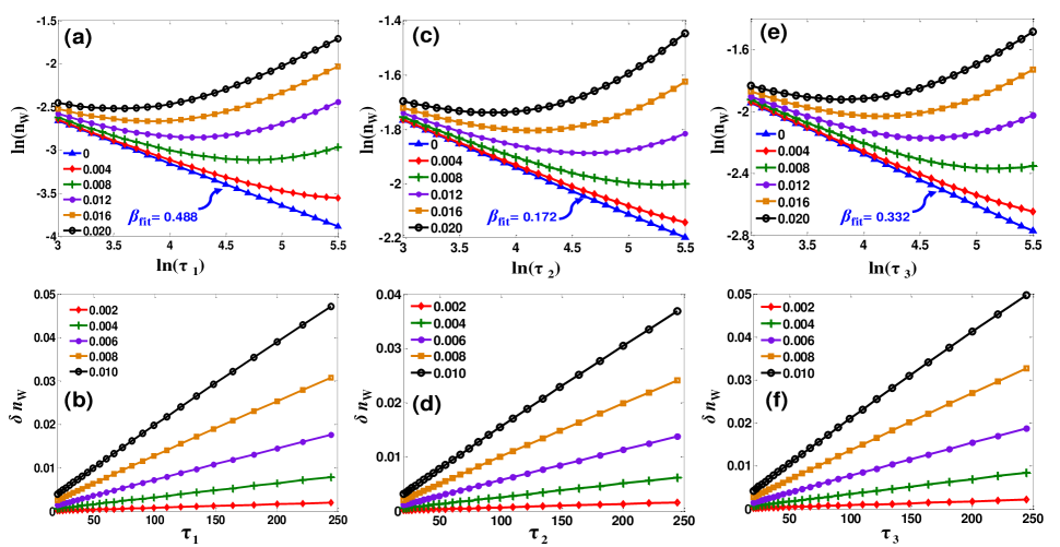
Figure 2(a) illustrates the numerical results of the defect density as a function of the quench time in the transverse quench protocol. When the driving field is free from noises with , the results of with the fitting exponent agrees well with the theoretical prediction of Kibble-Zeruk scaling exponent in the thermodynamical and long quench time limits Xy1 ; XyMC ; Xy2 . Note that the deviation of (about ) here comes from the finite size of -modes ( is set) and the finite quench time in our simulations. We have numerically confirmed that this deviation can be decreased with the increasing of and . For short quench time, the defect density as a function of the quench time is close to the scaling form in the noise-free case. As the strength of noise fluctuation grows (increasing ), the corresponding defect density increases compared to the results under noise-free condition, and the deviation becomes more significant for longer quench time, where the dynamics is dominated by the noise-induced non-adiabatic effects. Then the power-law scaling form of fails and the system exhibits the anti-KZ behavior, i.e., slower driving (larger ) results in more defects. Finally is completely governed by the anti-KZ contribution in the limit of very long quench time.
The physics of the anti-KZ behavior can be further interpreted as follows: The defect production of the noise-free part of the quench system is due to the critical slowing down in KZM. In contrast, the noisy fluctuations in the control fields allow the absorption of energy to generate excitations in the system, which accumulate during the evolution with the increasing of the quench time. Thus, the resulting defect production is determined by the two independent mechanisms. For the relatively weak noises considered in our work, the noises contribute negligible excitations for the short quench time and then the scaling of the defect production is still effectively governed by the Kibble-Zurek predictions. When the quench time becomes large enough, the accumulation of noise-induced excitations dominates and the system enters the anti-KZ regime.
We proceed to consider the second quench protocol (), the anisotropic quench across the multicritical point with the control field and fixed , as shown in Fig. 1. In this case, the Hamiltonian for each -mode can be written as , where
| (13) |
Here the linearly driving field with the quench velocity . Similar to the first protocol mentioned above, in our numerical simulations, we choose and , and let ramp from to with the overall quench time . Under this condition, the system is initially in the PM phase and then driven through the multicritical point into the FMx phase. Consequently, the quench velocity , and the evolution progress is . Figure 2(c) shows the numerical results of the defect density in this quench protocol. In the noise-free limit with , we find that with the fitting exponent agrees with the theoretical prediction Xy1 ; XyMC ; Xy2 . When the dynamics is dominated by the noise effects for increasing the noise strength and (or) quench time, this power-law scaling again fails and the system exhibits the anti-KZ behavior.
For the last quench protocol along the gapless line protocol (), the parameter is used as the control field to linearly drive the system, which takes the form in the evolution progress . The other parameters are set as . Therefore, the Hamiltonian for each -mode in this case is , where the two parts
| (14) |
The numerical results of the defect density in this quench protocol are shown in Fig. 2(e). For , we find that with the fitting scaling exponent consistent with the theoretical prediction Xy1 ; XyMC ; Xy2 . Increasing the noise strength , the system inters the anti-KZ regime, with more defects formed for longer quench time. Hence, we come to the conclusion that when the noises presents in the control fields, the anti-KZ behavior exists in all the three quench protocols in the transverse-field XY chain with different noise-free Kibble-Zeruk scaling exponents.
Due to the exhibition of the anti-KZ behavior in the quench when the noise presents, it is imperative to find an optimal quench time to minimize the defects. Under the condition of finite quench time , the optimal control in the annealing of quantum simulator give a challenge that defect (excitation) density is produced as less as possible. For our numerical results, we focus on the region , since the experimental systems only maintain their quantum coherent characteristic in finite ramp time. As the defect density in the absence of noises , where the prefactor is predicted by KZM and depends on s specific protocol. One can argue that in the limit of small noise and finite quench time Dutta , the total density of defect , where the noised-induced part is given by
| (15) |
Note that the effective decoupling of the KZM dynamics from noise-induced effects, as interpreted previously, leads to the additive form of . Figure 2(b,d,f) display that for the three quench protocols () is almost linearly depend on when , and thus one has
| (16) |
with being the coefficient whose value depends on the noise strength. Secondly, the optimal quench time can be derived approximately by minimizing in Eq. (15), which is then given by Dutta
| (17) |
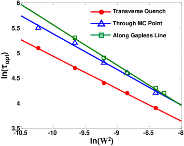
This relation is verified to be applicable for all the three quench protocols in the parameter regions we considered, as illustrated in Fig. 3. In the original KZM scenario, only the control fields without noises accounts for the production of defect and long quench time prevents defects formation. However, we have shown that the noises in the control fields, which is a more practical situation in realistic experiments, can also induce defects and it is intuitively to use shorter quench time as optimum to suppress the defect production when noise strength gets larger.
III Quantum simulation of the anti-KZ behavior in two-level systems
In this section, we propose to test the predicted anti-KZ behavior by quantum simulation of the quench dynamics with LZT in two-level systems. We first present a method to transform a generic two-level Hamiltonian with time linearly dependent term in the diagonal term into a standard LZT form. In a two-level system, the Schrödinger equation for the state vector with and as the diabatic basis can be written as
| (24) |
Here we assume the parameters and are real constants. We further use the substitution
| (25) |
into the origin two-level system Hamiltonian (24), which can then be transformed into the standard LZT form,
| (32) |
The probability in the excited state at the end of the driving is approximately given by the Landau-Zener formula Landau ; Zener ; Shevchenko .
On the other hand, KZM can be used to study the dynamics in the quantum phase transition driven across the quantum critical point. The essence of KZM is the adiabatic impulse approximation LZKZM1 , where the quench process is divided into three stages: adiabatic far away from the critical point, frozen state in the vicinity of the point when with denoting the freeze-out time scale, and the restart of adiabatic process. For convention, we define the relaxation time as , where is the energy gap between the ground state and the first excited state, and is estimated with and . Let , the impulse region is given by Isingexact1 . When the starting and ending points of in the Landau-Zener Hamiltonian is outside the impulse region, it can be regarded that there is a complete LZT in this two-level system. The similarity between LZT and KZM was firstly point out in LZKZM1 , one of the most prominent features is that when the system approaches the critical point, the inverse of the energy gap tends to infinity in KZM and the counterpart in LZT also increases.
The defect density can also be estimated by the integral of the transition probability over the pseudo-momentum space LZKZMexp_QD ; LZKZMexp_SC ; LZKZMexp_Ion
| (33) |
which can be measured in two-level systems by means of quantum simulation of the quench dynamics with well-designed Landau-Zener crossings, similar as the experiments for the Ising chain without noises LZKZMexp_QD ; LZKZMexp_SC ; LZKZMexp_Ion . For the three quench protocols in the noisy XY chain, the parameters in (24) for a two-level system correspond to the counterparts in the Hamiltonian of the noise-free quench for the three protocols). In addition, the noise part correspond to stochastic fluctuations of the control fields , which can be realized by inducing the or (and) fluctuations with tunable strength into the two-level systems.
To simulate the transverse quench () in transverse field XY chain with many independent LZT in pseudo-momentum space, one can use the mapping , and . This indicates the substitution in this quench protocol
| (34) |
which can transform into the standard LZT form. For the second quench protocol () of anisotropic quench through the multicritical point, following the mapping of the parameters similar as those in the first case, one can obtain the corresponding substitution
| (35) | |||||
Similarly, for the third quench protocol () along the gapless line, the mapping of the Hamiltonian in pseudo-momentum space gives the corresponding substitution
| (36) |
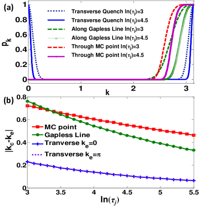
To reduce the number of implementing LZT in the estimation of the predicted , we consider the distribution of the excitation probability as a function of . The results for the three protocols with typical quench time are plotted in Fig. 4(a). One can find that only those modes in the regions near the points and (or) contribute the major to the excitation formation. Therefore in experiments, one can just implement some LZT of the modes in these regions to extract the simulated defect density. For practical implementation, one may define a cutoff pseudo-momentum in quantum simulation, which separates the axis into two or three (for transverse quench) parts determined by the excitation probability here (other small values are also applicable). Figure 4(b) depicts as a function of the quench time in the three protocols, which approximately gives the length of the required simulation regions measured from the point . The results also show that the region length monotonously decreases as increasing .
IV conclusions
In summary, we have studied the quench dynamics of a transverse-field XY chain driven across quantum critical points by noisy control fields and demonstrated that the defect productions for three quench protocols with different scaling exponents exhibit the anti-KZ behavior. We have also shown that the optimal quench time to minimize defects scales as a universal power law of the noise strength for all the three cases. Moreover, by using quantum simulation of the quench dynamics in the spin system with well-designed Landau-Zener crossings in pseudo-momentum space, we have proposed an experimentally feasible scheme to test the predicted anti-KZ behavior.
Acknowledgements.
This work was supported by the NKRDP of China (Grant No. 2016YFA0301803), the NSFC (Grants No. 11604103, No. 11474153, and No. 91636218), the NSF of Guangdong Province (Grant No. 2016A030313436), and the Startup Foundation of SCNU.References
- (1) T. W. B. Kibble, Topology of cosmic domains and strings, J. Phys. A 9, 1387 (1976).
- (2) W. H. Zurek, Cosmological experiments in superfluid helium, Nature 317, 505 (1985).
- (3) W. H. Zurek, Cosmological experiments in condensed matter systems, Phys. Rep. 276, 177 (1996).
- (4) N. Navon, A.L. Gaunt, R.P. Smith, and Z. Hadzibabic, Critical dynamics of spontaneous symmetry breaking in a homogeneous Bose gas, Science 347, 167 (2015) .
- (5) S. Ulm, J. Ronagel, G. Jacob, C. Degünther, S. T. Dawkins, U. G. Poschinger, R. Nigmatullin, A. Retzker, M. B. Plenio, F. Schmidt-Kaler, and K. Singer, Observation of the Kibble-Zurek scaling law for defect formation in ion crystals, Nat. Commun. 4, 2290 (2013).
- (6) K. Pyka, J. Keller, H. L. Partner, R. Nigmatullin, T. Burgermeister, D. M. Meier, K. Kuhlmann, A Retzker, and M. B. Plenio, Topological defect formation and spontaneous symmetry breaking in ion Coulomb crystals, Nat. Commun. 4, 2291 (2013).
- (7) R. Monaco, J. Mygind, and R. J. Rivers, Zurek-Kibble Domain Structures: The Dynamics of Spontaneous Vortex Formation in Annular Josephson Tunnel Junctions,Phys. Rev. Lett. 89, 080603 (2002).
- (8) J. Dziarmaga, Dynamics of a quantum phase transition and relaxation to a steady state, Adv. Phys. 59, 1063 (2010).
- (9) J. Dziarmaga, Dynamics of a quantum phase transition: Exact solution of the quantum Ising model, Phys. Rev. Lett. 95, 245701(2005).
- (10) W. H. Zurek, U. Dorner, and P. Zoller, Dynamics of a quantum phase transition, Phys. Rev. Lett. 95, 105701 (2005).
- (11) J. Dziarmaga, Dynamics of a quantum phase transition in the random Ising model: logarithmic dependence of the defect density on the transition rate, Phys. Rev. B 74, 064416 (2006).
- (12) T. Caneva, R. Fazio, and G. E. Santoro, Adiabatic quantum dynamics of a random Ising chain across its quantum critical point, Phys. Rev. B 76, 144427 (2007).
- (13) V. Mukherjee, U. Divakaran, A. Dutta, and D. Sen, Quenching dynamics of a quantum XY spin- chain in a transverse field, Phys. Rev. B 76, 174303 (2007).
- (14) U. Divakaran, V. Mukherjee, A. Dutta, and D. Sen, Defect production due to quenching through a multicritical point, J. Stat. Mech. P02007 (2009).
- (15) U. Divakaran, A. Dutta, and D. Sen, Quenching along a gapless line: A different exponent for defect density, Phys. Rev. B 78, 144301 (2008).
- (16) S. Deng, G. Ortiz, and L. Viola, Dynamical non-ergodic scaling in continuous finite-order quantum phase transitions, Eurphys. Lett. 84, 67008 (2009).
- (17) J. Sabbatini, W. H. Zurek, and M. J. Davis, Phase Separation and Pattern Formation in a Binary Bose-Einstein Condensate, Phys. Rev. Lett. 107, 230402 (2011).
- (18) M. Kolodrubetz, B. K. Clark, and D. A. Huse, Nonequilibrium Dynamic Critical Scaling of the Quantum Ising Chain, Phys. Rev. Lett. 109, 015701 (2012).
- (19) T. Caneva, R. Fazio, and G. E. Santoro, Adiabatic quantum dynamics of the Lipkin-Meshkov-Glick model, Phys. Rev. B 78, 104426(2008).
- (20) O. L. Acevedo, L. Quiroga, F. J. Rodr guez, and N. F. Johnson, New dynamical scaling universality for quantum networks across adiabatic quantum phase transitions, Phys. Rev. Lett. 112, 030403 (2014).
- (21) S. Sachdev, Quantum Phase Transitions (Cambridge University Press, Cambridge, England, 1999).
- (22) D. Chen, M. White, C. Borries, and B. DeMarco, Quantum Quench of an Atomic Mott Insulator, Phys. Rev. Lett. 106, 235304 (2011).
- (23) S. Braun, M. Friesdorf, S. S. Hodgman, M. Schreiber, J. P. Ronzheimer, A. Riera, M. del Rey, I. Bloch, J. Eisert, and U. Schneider, Emergence of coherence and the dynamics of quantum phase transitions, Proc. Natl. Acad. Sci. 112, 3641 (2015).
- (24) M. Anquez, B. A. Robbins, H.M Bharath, M. Boguslawski, T. M. Hoang, and M. S. Chapman, Quantum Kibble-Zurek Mechanism in a Spin-1 Bose-Einstein Condensate, Phys. Rev. Lett. 116, 155301 (2016).
- (25) L. W. Clark, L. Feng, and C. Chin, Universal space-time scaling symmetry in the dynamics of bosons across a quantum phase transition, Science 354, 606 (2016).
- (26) L. D. Landau, On the theory of transfer of energy at collisions II. Physik. Z. Sowjet. 2, 46 (1932).
- (27) C. Zener, Non-adiabatic crossing of energy levels. Proc. R. Soc. London, Ser. A 137, 696 (1932).
- (28) S. N. Shevchenko, S. Ashhab, and F. Nori, Landau-Zener-St ckelberg interferometry. Phys. Rep. 492, 1 (2010).
- (29) W. D. Oliver, Y. Yu, J. C. Lee, K. K. Berggren, L. S. Levitov, and T. P. Orlando, Mach-Zehnder interferometry in a strongly driven superconducting qubit. Science 310, 1653 (2005).
- (30) M. Sillanpaa, T. Lehtinen, A. Paila, Y. Makhlin, and P. Hakonen, Continuous-time monitoring of Landau-Zener interference in a cooper-pair box. Phys. Rev. Lett. 96, 187002 (2006).
- (31) X. Tan, D.-W. Zhang, Z. Zhang, Y. Yu, S. Han, and S.-L. Zhu, Demonstration of Geometric Landau-Zener Interferometry in a Superconducting Qubit. Phys. Rev. Lett. 112, 027001 (2014).
- (32) J. R. Petta, H. Lu, and A. C. Gossard, A Coherent Beam Splitter for Electronic Spin States, Science 327, 669 (2010).
- (33) C. Betthausen, T. Dollinger, H. Saarikoski, V. Kolkovsky, G. Karczewski, T. Wojtowicz, K. Richter, and D. Weiss, Spin-transistor action via tunable Landau-Zener transitions, Science 337, 324 (2012).
- (34) G. Cao, H.-O. Li, T. Tu, L. Wang, C. Zhou, M. Xiao, G.-C. Guo, and H.-W. Jiang, Ultrafast universal quantum control of a quantum-dot charge qubit using Landau-Zener-Stückelberg interference, Nat. Commun. 4, 1401 (2013).
- (35) L. Tarruell, D. Greif, T. Uehlinger, G. Jotzu, and T. Esslinger, Creating, moving and merging Dirac points with a Fermi gas in a tunable honeycomb lattice. Nature 483, 302 (2012).
- (36) T. Salger, C. Geckeler, S. Kling, and M. Weitz, Atomic Landau-Zener tunneling in Fourier-synthesized optical lattices. Phys. Rev. Lett. 99, 190405 (2007).
- (37) Y.-A. Chen, S. D. Huber, S. Trotzky, I. Bloch, and E. Altman, Many-body Landau-Zener dynamics in coupled one-dimensional Bose liquids. Nat. Phys. 7, 61 (2011).
- (38) B. Damski, The simplest quantum model supporting the Kibble-Zurek mechanism of topological defect production: Landau-Zener transitions from a new perspective, Phys. Rev. Lett. 95, 035701 (2005).
- (39) B. Damski and W. H. Zurek, Adiabatic-impulse approximation for avoided level crossings: From phase-transition dynamics to Landau-Zener evolutions and back again. Phys. Rev. A 73, 063405 (2006).
- (40) X.-Y. Xu, Y.-J. Han, K. Sun, J.-S. Xu, J.-S. Tang, C.-F. Li, and G.-C. Guo, Quantum simulation of Landau-Zener model dynamics supporting the Kibble-Zurek mechanism. Phys. Rev. Lett. 112, 035701 (2014).
- (41) L. Wang, C. Zhou, T. Tu, H.-W. Jiang, G.-P. Guo, and G.-C. Guo, Quantum simulation of the Kibble-Zurek mechanism using a semiconductor electron charge qubit, Phys. Rev. A. 89, 022337 (2014).
- (42) M. Gong, X. Wen, G. Sun, D.-W. Zhang, D. Lan, Y. Zhou, Y. Fan, Y. Liu, X. Tan, H. Yu, Y. Yu, S.-L. Zhu, S. Han, and P. Wu, Simulating the Kibble-Zurek mechanism of the Ising model with a superconducting qubit system, Sci. Rep. 6, 22667 (2016).
- (43) J.-M. Cui, Y.-F. Huang, Z. Wang, D.-Y. Cao, J. Wang, W.-M. Lv, L. Luo, A. del Campo, Y.-J. Han, C.-F. Li, and G.-C. Guo, Experimental Trapped-ion Quantum Simulation of the Kibble-Zurek dynamics in momentum space, Sci Rep. 6, 33381 (2016).
- (44) S. M. Griffin, M. Lilienblum, K. T. Delaney, Y. Kumagai, M. Fiebig, and N. A. Spaldin, Scaling behavior and beyond equilibrium in the hexagonal manganites, Phys. Rev. X 2, 041022(2012).
- (45) E. A. Novikov, Functionals and the random-force method in turbulence theory, JETP, 20, 1290 (1965).
- (46) D. Patanè, A. Silva, L. Amico, R. Fazio, and G. E. Santoro, Adiabatic Dynamics in Open Quantum Critical Many-Body Systems, Phys. Rev. Lett. 101, 175701 (2008).
- (47) P. Nalbach, S. Vishveshwara, and A. A. Clerk, Quantum Kibble-Zurek physics in the presence of spatially correlated dissipation, Phys. Rev. B 92, 014306 (2015).
- (48) A. Dutta, A. Rahmani, and A. del Campo, Anti-Kibble-Zurek Behavior in Crossing the Quantum Critical Point of a Thermally Isolated System Driven by a Noisy Control Field, Phys. Rev. Lett. 117, 080402 (2016).
- (49) A. Rahmani, Dynamics of noisy quantum systems in the Heisenberg picture: Application to the stability of fractional charge, Phys. Rev. A 92, 042110 (2015).
- (50) K. Kim, M. S. Chang, S. Korenblit, R. Islam, E. E. Edwards, J. K. Freericks, G. D. Lin, L. M. Duan, and C. Monroe, Quantum simulation of frustrated Ising spins with trapped ions, Nature 465, 590 (2010).
- (51) J. G. Bohnet, B. C. Sawyer, J. W. Britton, M. L. Wall, A. M. Rey, M. Foss-Feig, and J. J. Bollinger, Quantum spin dynamics and entanglement generation with hundreds of trapped ions, Science 352, 1297 (2016).
- (52) J. Simon, W. S. Bakr, R. Ma, M. E. Tai, P. M. Preiss, and M. Greiner, Quantum simulation of antiferromagnetic spin chains in an optical lattice, Nature 472, 307 (2011).
- (53) E. Lieb, T. Schultz, and D. Mattis, Two soluble models of an antiferromagnetic chain, Ann. Phys. (N.Y.) 16, 407 (1961).
- (54) J. E. Bunder and Ross H. McKenzie, Effect of disorder on quantum phase transitions in anisotropic XY spin chains in a transverse field, Phys. Rev. B 60, 344 (1999)